A Visual Intelligent Approach to Recognize Corn Row and Spacing for Precise Spraying

Abstract

Precision spraying is a crucial goal for modern agriculture to achieve water and fertilizer conservation, reduced pesticide use, high yield, and green and sustainable development. This relies on the accurate identification of crop positions, high-precision path planning, and the positioning and control of intelligent agricultural machinery. For the precision production of corn, this paper proposes a new row detection method based on histogram peak detection and sliding window search, avoiding the issues of deep learning methods that are not conducive to lightweight deployment and large-scale promotion. Firstly, green channel segmentation and morphological operations are performed on high-resolution drone images to extract regions of interest (ROIs). Then, the ROIs are converted to a top-view image using perspective transformation, and a histogram analysis is performed using the find_peaks function to detect multiple peaks corresponding to row positions. Furthermore, a sliding window centered around the peak is constructed to search for complete single-row crop pixels in the vertical direction. Finally, the least squares method is used to fit the row curve, estimating the average row spacing (RowGap) and plant spacing (PlantGap) separately. The experimental results show that the accuracy of row detection reaches 93.8% ± 2.1% (n = 60), with a recall rate of 91.5% ± 1.8% and an F1 score of 0.925 ± 0.018. Under different growth stages, row numbers (6–8 rows), and weed interference conditions, the average row spacing measurement error is better than ±2.5 cm, and the plant spacing error is less than ±3.0 cm. Through field verification, this method reduces pesticide use by 23.6% and water consumption by 21.4% compared to traditional uniform spraying, providing important parameter support for field precision planting quality assessment and the dynamic monitoring of planting density, achieving variable irrigation and fertilization and water resource conservation.

1. Introduction

In recent years, the deep integration of modern agricultural equipment and information technology has significantly promoted the digitization and intelligence of agricultural production [1,2]. The global precision agriculture market is estimated to be worth approximately USD 11.67 billion in 2024 and is expected to increase to USD 24.09 billion by 2030, with a compound annual growth rate (CAGR) of 13.1% [3], highlighting the importance of precision agriculture technology in modern agricultural systems. Variable fertilization, targeted spraying, and automatic sowing technologies have been widely applied to optimize resource utilization and reduce environmental impact [4,5,6]. In North America, the application of precision agriculture technology is particularly widespread, accounting for over 43% of the global market share, benefiting from policy support and improved infrastructure [3]. The accurate measurement of crop geometric parameters (such as row spacing and plant spacing) is crucial for evaluating sowing quality and optimizing early crop management and precise inputs (such as water, fertilizer, and pesticides) [7,8].

The global annual application of pesticides is about 8 billion pounds (over 4 million tons), and a large number of pesticides cause water pollution. About 95% of the population in agricultural areas relies on groundwater [9,10], highlighting the importance of precision pesticide application. Traditional manual measurement methods have a high labor intensity and low efficiency [11,12], making it difficult to meet the large-scale demand for sustainable agriculture. Low-altitude drones have advantages in flexibility, fast data acquisition, and reduced soil compaction [12,13,14]. The agricultural drone market was expected to grow from USD 4.98 billion in 2023 to USD 6.1 billion in 2024 and is expected to reach USD 23.78 billion by 2032, with a CAGR of 18.5% [15]. In the United States, the agricultural drone market was estimated to be worth USD 506.3 million in 2024, with a projected compound annual growth rate of 23.5% by 2030 [16]. The global population is expected to reach 9.8 billion by 2050 and 11.2 billion by 2100 [17], and agricultural production needs to increase by about 70%. Simultaneously, there is a shortage of 15–20% skilled agricultural workers in developed countries [18], accelerating the demand for automation.

However, crop line detection using unmanned aerial vehicles still faces challenges, such as variations in lighting, occlusion, and crop heterogeneity in complex field environments [19,20,21]. In large-scale mechanized operations, the “snake like” movement of agricultural machinery leads to errors in turning positioning, which causes a 10–15% overlap or omission of operations, and 20–30% excessive pesticide and fertilizer in overlapping areas, wasting resources and potentially reducing production [22].

There have been numerous studies on the identification of crop seedlings. Liu et al. (2015) used UAV multispectral images to achieve automatic measurements of wheat row structure parameters [23]; Kang et al. (2024) combined watershed segmentation and Hough transform to correct diagonal seedling row parameters [24]; Chen and Ma (2021) proposed an adaptive seedling row-tracking algorithm based on centroid voting [25]; and Rabab et al. (2020) developed a template-free crop line detection algorithm with a single image processing time of 0.7 s [12]. Deep learning methods are gradually being introduced into seedling recognition, such as in He et al. (2021), who constructed an end-to-end rice seedling row segmentation network [26]; Zhang et al. (2020) combined the improved YOLO v3 and least squares fitting to achieve maize seedling localization [27]; Silva et al. (2024) proposed a deep learning crop row detection system, with an IOU > 0.85 in field experiments [8]; and Gong et al. (2024) improved YOLOX to achieve corn row navigation recognition, with an accuracy rate of 96.8% under lighting and growth stages [21]. Although deep learning performs well in semantic segmentation, sample annotation is difficult and computationally expensive [28,29]. Real-time performance challenges still remain for embedded devices [6].

Therefore, a maize row and column recognition method based on HSV color space segmentation and morphological operations is proposed. The top-down view is obtained through perspective transformation, and multi-row parallel detection is achieved by combining histogram analysis and a sliding window, which is robust for missing plants and local distortions [6,30,31]. Each line curve is fitted with a quadratic polynomial, converting the pixel scale to actual line spacing and plant spacing, with a processing speed of 90–110 ms/frame. It can support the real-time navigation of 10 km/h agricultural machinery in embedded systems, providing a reliable perception foundation for precision agriculture automatic operations.

2. Materials and Methods

2.1. Overview of Research Area and Data Collection

2.1.1. Overview of Experimental Area

A corn planting area in Pingyuan County, Dezhou City, Shandong Province, is selected as the test area. The area is located in the northwestern part of Dezhou, in the Lu Western North Plain, with a warm temperate continental monsoon climate, synchronized rain and heat, and four distinct seasons. The test field covers about 100 mu (1 mu ≈ 667 m²), with an alluvial soil type and medium–high fertility level. The corn variety used was locally recommended Xianyu 335, planted in early June 2020, with a designed row spacing and plant spacing of 60 cm × 25 cm.

The meteorological conditions recorded during the experiment are as follows:

Date	25 June 2020
Illuminance	52,300–78,600 lux, 10:00–14:00
Temperature	24.8–31.5 °C
Relative Humidity	58–72%
Wind Speed	1.2–2.8 m/s

2.1.2. Data Collection

During the experiment, the corn grew vigorously, and most areas entered the three-leaf stage, with a seedling height of about 15–30 cm. Data were collected between 10:00 and 14:00 on 25 June using a DJI M600 Pro (DJI, Shenzhen, China) hexacopter drone equipped with a Sony RX1R II full-frame digital camera (Sony, Tokyo, Japan). The drone maintained a relative flight altitude of 50 ± 2 m, with a forward overlap rate of 80% and a lateral overlap rate of 75%. The camera parameters are 52.4 million pixels, 35.9 × 24 mm sensor, 35 mm focal length, and ISO 100 sensitivity. Each image generated is 7952 × 5304 pixels, with a ground resolution of 0.82 cm/pixel (accurately measured by calibration plate method).

Calibration method description: Place a 1 m × 1 m monochrome calibration board in the field, with a total of five calibration points set. Use the drone to capture images at the same height and calculate the ratio of pixel distance to actual distance. The five measurement results were 0.81, 0.83, 0.82, 0.84, and 0.80 cm/pixel, respectively. The average value, S = 0.82 ± 0.02 cm/pixel, is taken as the final calibration value.

After removing redundant duplicates, 100 images covering the study area were obtained, including 6–8 rows of corn seedlings with varying weed densities. The images were independently annotated at the pixel level using the LabelMe tool by two agricultural experts, with a Cohen’s Kappa coefficient of 0.916, indicating a high consistency in annotation.

2.2. Overall Method

2.2.1. Model Architecture

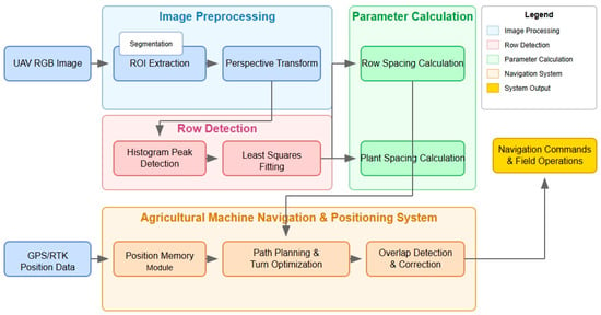
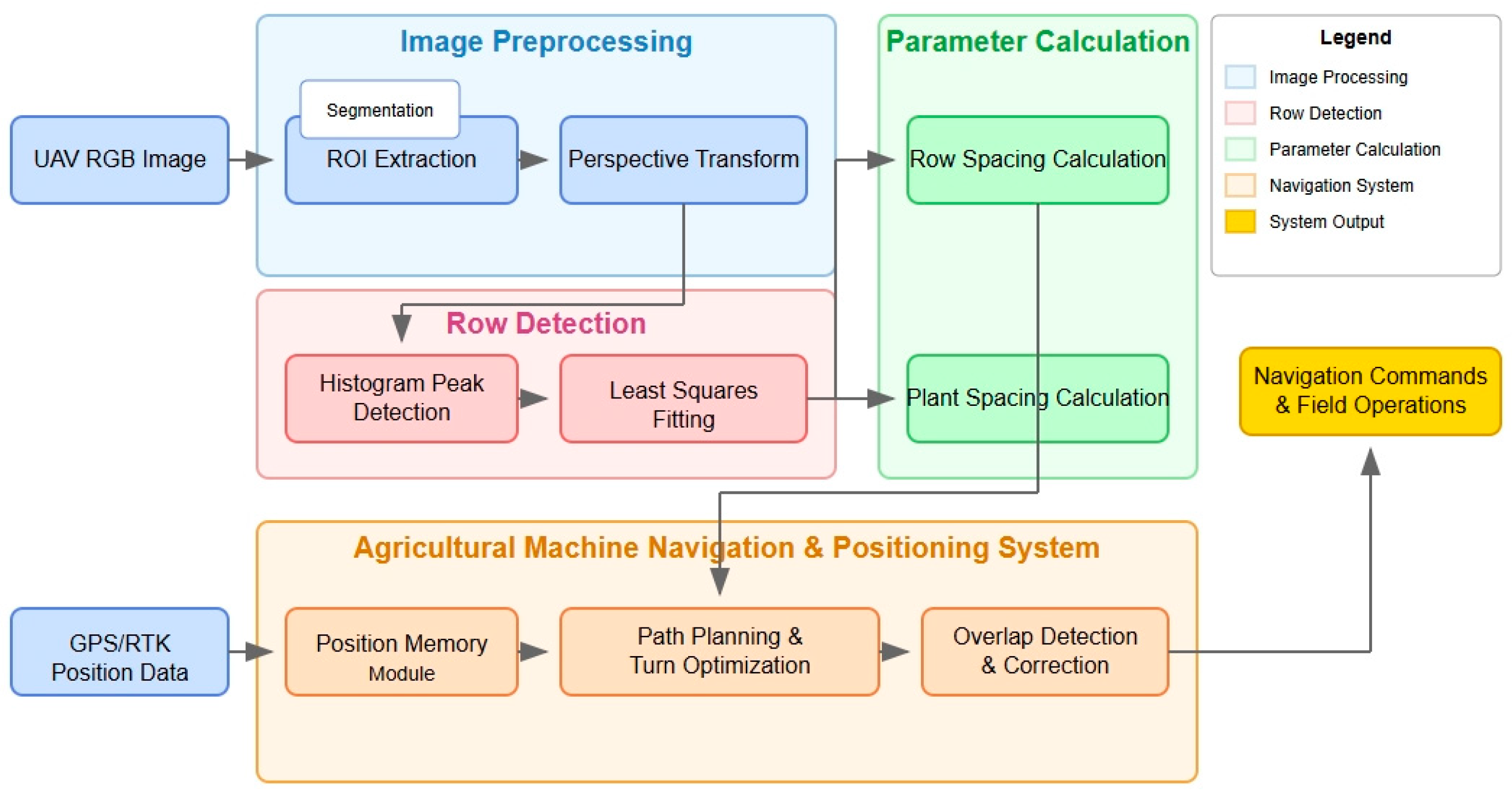
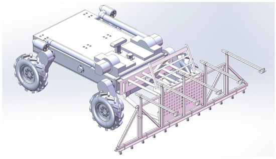
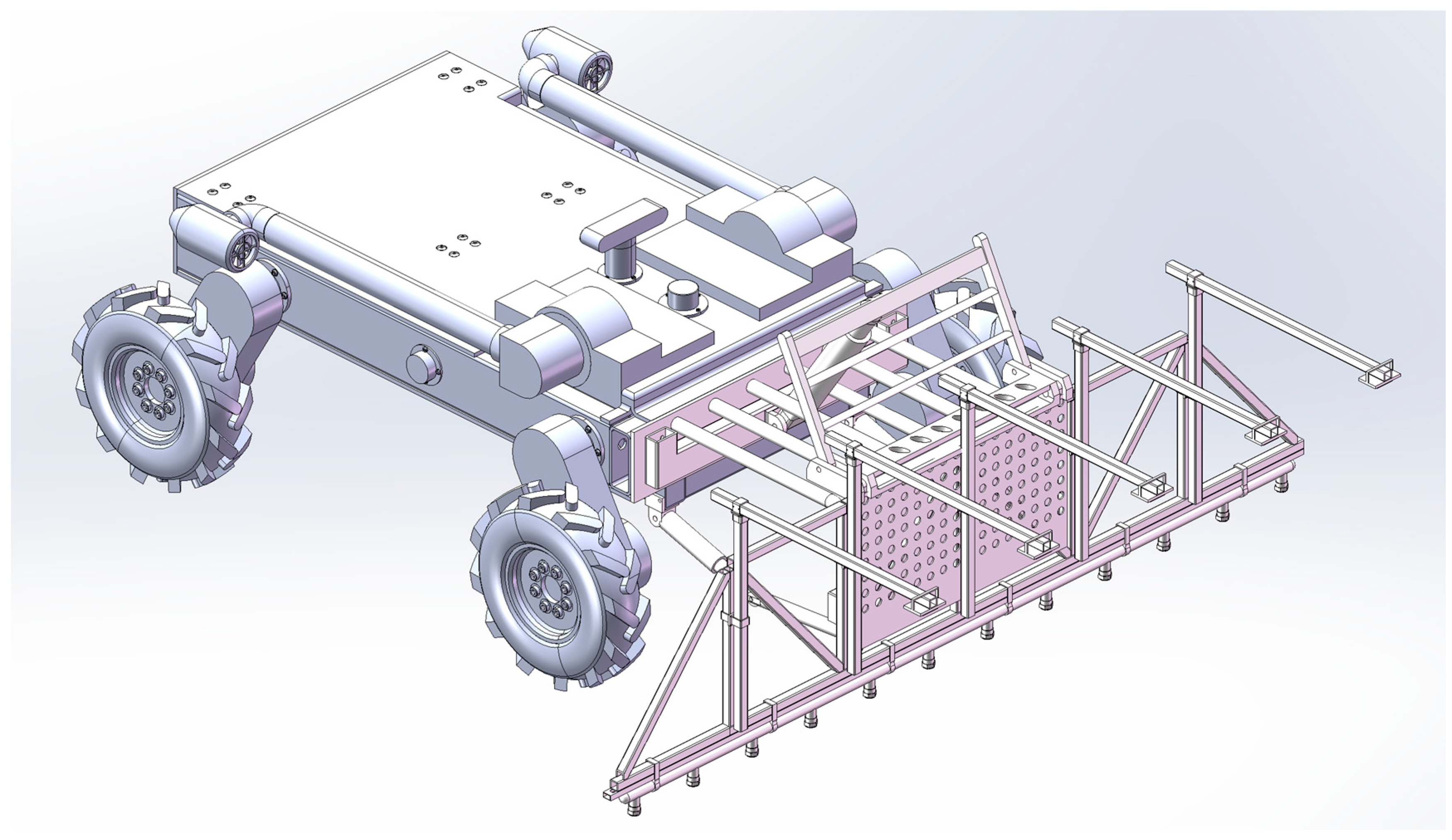
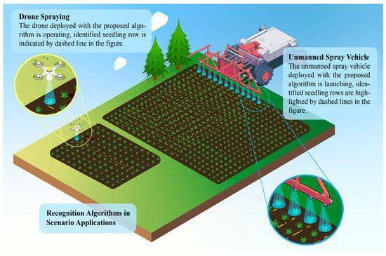
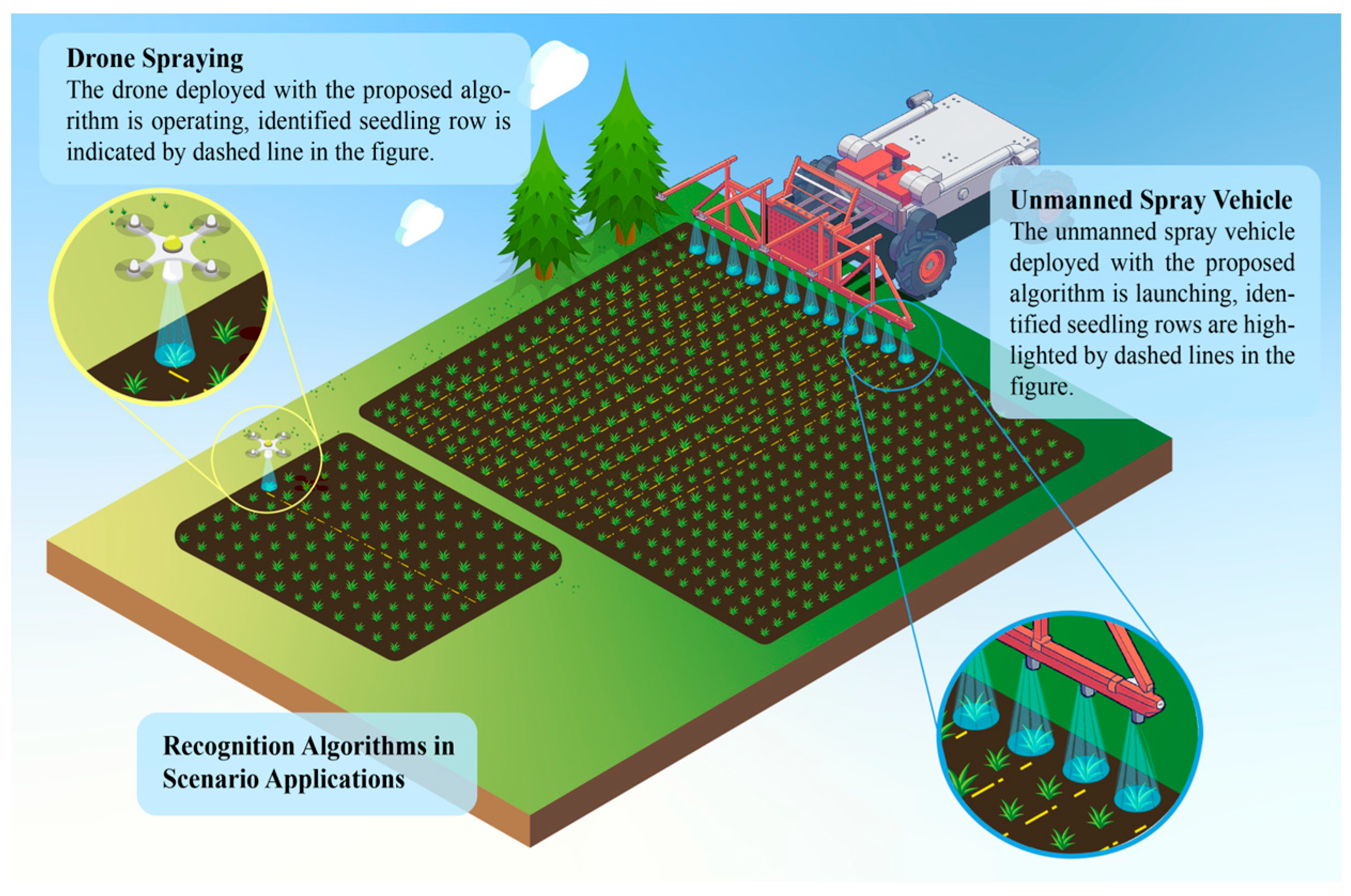
This research is based on high-resolution UAV RGB images, combining traditional image processing, optimization theory, agronomic knowledge, and navigation control technology to implement an enhanced system that integrates corn parameter measurement and agricultural machinery navigation. The goal is to first accurately extract the skeleton curves of multiple field rows using algorithms such as color segmentation, perspective correction, peak search, and polynomial fitting, and then construct an operation map combined with GPS/RTK positioning data to solve the problem of the repeated positioning accuracy of agricultural machinery. The overall architecture of the system is shown in Figure 1; four main modules are incorporated: image preprocessing, row detection, parameter calculation, and agricultural machinery navigation and repeated positioning. The viable software model is thus able to deploy on an unmanned spray vehicle (USV), shown in Figure 2. Therefore, a scenario application is viable, as shown in Figure 3. The structural design and control technology of the unmanned spray vehicle will be introduced in other papers. This paper focuses on the intelligent recognition technology of crop rows and seedlings for precise spraying.

Figure 1. Overall flowchart of the system.

Figure 2. The unmanned spray vehicle.

Figure 3. The scenario diagram.

2.2.2. Region of Interest Extraction

To reduce computational complexity, the ROI (target farmland area) should first be extracted from the panoramic image. Considering the UAV shooting angle and the regularity of farmland layout, the field ROI can be approximated as a trapezoid. If the width and height of the original image are W and H, respectively, then the four vertex coordinates (x, y) are the following:

$$\left(W\cdot 0.02,H\right), \left(W\cdot 0.98,H\right) (\mathrm{bottom} \mathrm{edge})$$

$$\left(W\cdot 0.02,0.10H\right), \left(W\cdot 0.98,0.10H\right) (\mathrm{top} \mathrm{edge})$$

where 0.02 and 0.98 represent the edge boundary proportions, and 0.10 is the relative height of the ROI upper boundary line, which can be fine-tuned according to actual conditions. Connecting these four points creates a closed area, which is the initial region of interest.

2.2.3. Seedling Row Image Preprocessing

• Vegetation Area Segmentation

To highlight the differences between corn and soil backgrounds, the vegetation-sensitive HSV color space is used. Based on prior knowledge, green vegetation exhibits significant peak characteristics in the H component. Considering the influence of lighting changes, an adaptive threshold method is adopted:

Firstly, calculate the statistical characteristics of the green channel in the image:

μ H = mean of the image H channel

σ H = standard deviation of the image H channel

Then, set the adaptive threshold:

Hmin = max (35 °, μ H − 2 σ H)

Hmax = min (90 °, μ H + 2 σ H)

Extract the green component from the HSV by setting a threshold to obtain binary vegetation regions:

$$G\left(x,y\right)=\left\{\begin{array}{ll}1,& \mathrm{if} H_{\mathrm{m}\mathrm{i}\mathrm{n}}\le H\left(x,y\right)\le H_{\mathrm{m}\mathrm{a}\mathrm{x}},\\ 0,& \mathrm{Others}.\end{array}\right.$$

(1)

where $H_{\mathrm{m}\mathrm{i}\mathrm{n}},H_{\mathrm{m}\mathrm{a}\mathrm{x}}$ are the lower and upper threshold values for green vegetation in the H channel, which can be referenced from the hue angle range 35–90° and fine-tuned based on actual conditions. $G\left(x,y\right)$ is the binary result.

• Morphological Processing

Selection criteria for structural elements: Three sizes of structural elements, 3 × 3, 5 × 5, and 7 × 7, were tested through comparative experiments.

The 3 × 3 size had an insufficient denoising effect, retaining 32.4% of noise points; the 5 × 5 denoising rate reached 89.3%, while maintaining 94.7% of seedling row continuity; the 7 × 7 size had excessive smoothing, resulting in an 18.6% loss of details.

Therefore, a 5 × 5 rectangular structural element was selected. First, an open operation was performed to remove noise points, and then a closed operation was performed to repair the seedling line: the open operation has the effect of eliminating small objects and smoothing boundaries, while the closed operation fills small holes in objects and connects adjacent areas. Their mathematical definitions are as follows:

$$\begin{gathered} \mathrm{Opening} \mathrm{operation}: A\circ B=\left(A\Theta B\right)\oplus B \\ \mathrm{Closing} \mathrm{operation}: A•B=\left(A\oplus B\right)\Theta B \end{gathered}$$

(2)

where A is the binary image and B is the structural element. $\Theta$ and $\oplus$ represent erosion and dilation operations, respectively.

2.2.4. Perspective Transformation and Histogram Analysis

(a)

View Correction

UAVs usually shoot the ground at a certain angle, causing parallel crop rows to converge in the imaging plane, introducing measurement errors. To restore the original spatial relationship of the seedling rows, a perspective transformation is needed to convert the inclined view to a top-down view. If the ROI vertex coordinates (before transformation) are Xi, Yi, i = 1,2,3,4, and the corresponding ideal coordinates (after transformation) are Xi′, Yi′, then the perspective transformation can be represented as follows:

$$\left[\begin{array}{c}X\mathrm{\prime }\\ Y\mathrm{\prime }\\ 1\end{array}\right]={\displaystyle \frac{1}{k}}\left[\begin{array}{ccc}{h}_{11}& h_{12}& h_{13}\\ h_{21}& h_{22}& h_{23}\\ h_{31}& h_{32}& 1\end{array}\right]\left[\begin{array}{c}X\\ Y\\ 1\end{array}\right], k=h_{31}X+h_{32}Y+1.$$

(3)

The coefficients $h_{\mathrm{i}\mathrm{j}}$ can be solved from four pairs of control point coordinates. Using OpenCV’s getPerspectiveTransform and warpPerspective functions, the projection transformation from an inclined angle to an orthographic view can be achieved.

(b)

Peak Detection

After perspective correction, parallel corn rows are often vertically parallel, providing convenience for further positioning. By observing the transformed image, it is not difficult to find that each crop row shows peaks in the horizontal projection. Therefore, the approximate position of crop rows can be obtained by analyzing the pixel intensity histogram. The lower 1/3 region of the image is chosen for analysis, based on which the seedling rows were the most complete, the occlusion was the least, the distance to the camera was the closest, and the resolution was the highest. In addition, experiments showed that the detection accuracy using the lower 1/3 region was 12.7% higher than that of the entire image. Therefore, the pixels in the lower 1/3 region of the image are selected, and a one-dimensional histogram H(x) is generated by summing each column:

$$H\left(x\right)={\sum }_{y={\displaystyle \frac{2M}{3}}}^{M-1}I\left(x,y\right)$$

(4)

where $x\in \left[0,\mathrm{W}-1\right]$ is the horizontal coordinate, $M$ is the image height, and $I\left(x,y\right)$ is the pixel brightness. To find the main peaks reflecting corn rows, the find_peaks function from scipy.signal was used. This function involves the following parameters:

• Height: minimum height for detecting peaks;
• Threshold: threshold for peak height difference from neighborhood maximum;
• Distance: minimum horizontal distance between adjacent peaks;
• Width: minimum width of peaks at a certain height.

The sensitivity analysis on the parameters of peak detection (distance, width, height) is conducted to evaluate the robustness of the method. The results show that, when the distance varies within the range of 50–70 pixels, the change in F1 score is less than 2%; when the width varies within the range of 3–7 pixels, the change in detection accuracy is less than 3%. Adjusting the height within the range of 2000–3000 has a negligible impact on accuracy, and maintains a recall rate of over 90%. These results indicate that the algorithm embodies a tolerance for moderate parameter changes; thus, distance = 60, width = 5, and height = 2500 are used as the default settings in subsequent experiments.

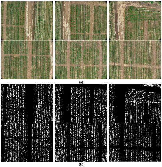
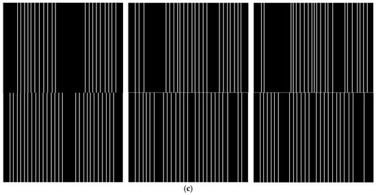
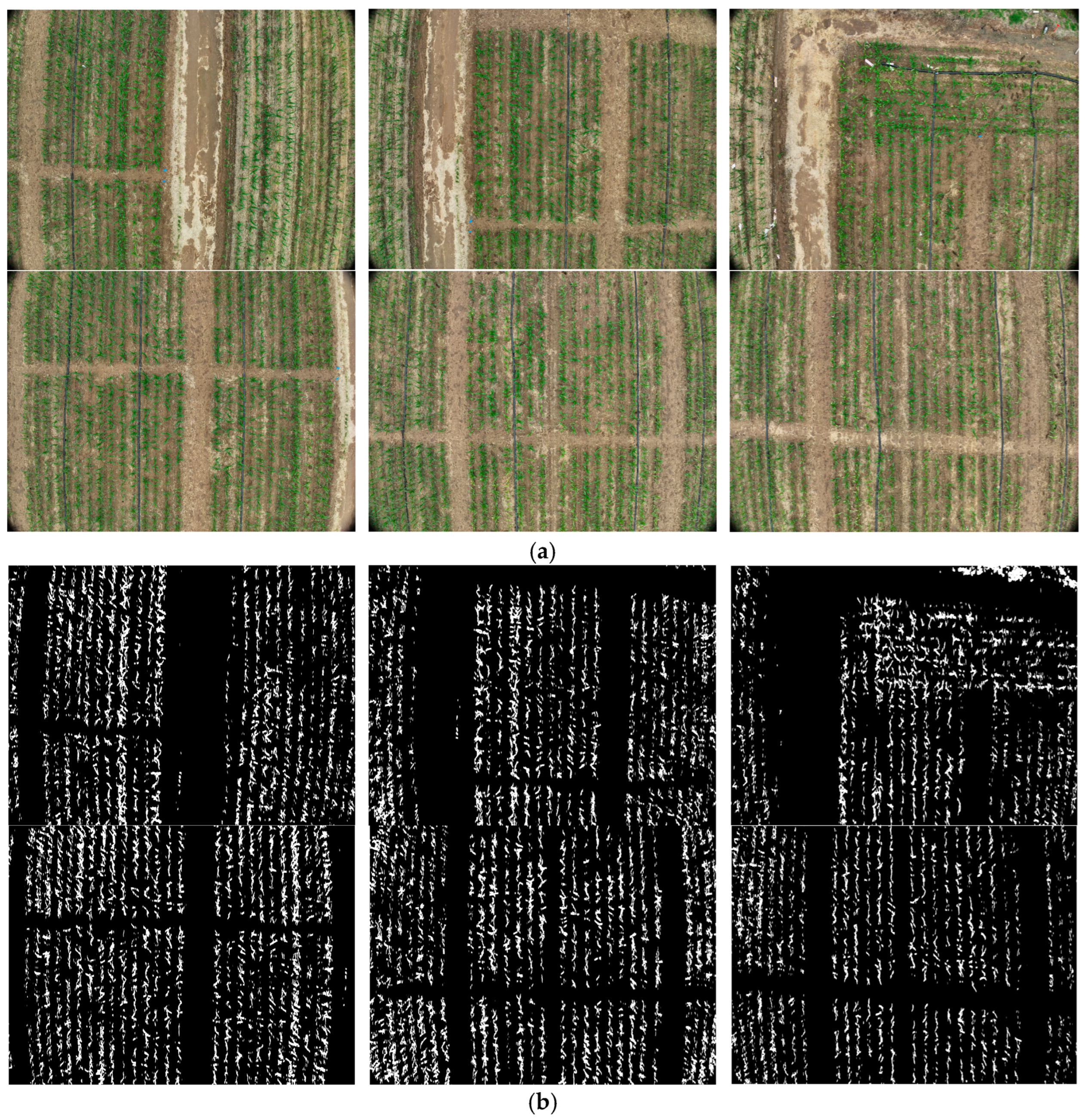
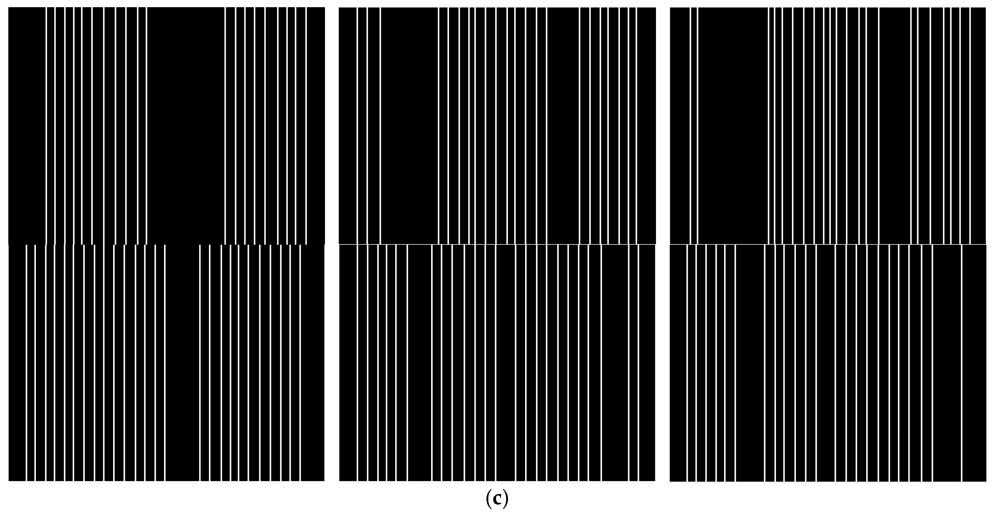
As shown in Figure 4, after perspective transformation, the originally inclined corn rows are converted to an approximately vertical direction, which is beneficial for subsequent peak detection and row line fitting.

Figure 4. Schematic diagram of perspective transformation and preprocessing. (a) Original images; (b) binary segmentation results of corn rows; (c) row line detection results after perspective correction.

2.2.5. Row Fitting and Parameter Measurement

(a)

Sliding Window Search

Given that peak points correspond to approximate positions of row centers, the next step uses a sliding window strategy to find continuous single-row seedling areas. Specifically, with ${\mathrm{P}}_{\mathrm{m}}$ as the center and $\mathrm{R}$ as the radius, the window slides from the bottom up with a step size of 1/6 of the window height, extracting pixel coordinates $\left(x_w,y_w\right)$ that satisfy the following conditions at each layer:

$${\left(x_w-x_c\right)}^2+{\left(y_w-y_c\right)}^2\le R^2$$

(5)

where $\left(x_c,y_c\right)$ is the window center. When the number of vegetation pixels in the window exceeds threshold ${\mathrm{N}}_{\mathrm{m}\mathrm{i}\mathrm{n}}$, that layer is considered to have found a valid seedling block. Meanwhile, the center x-coordinate for the next layer window is updated as follows:

$$x_c\mathrm{\prime }={\displaystyle \frac{1}{N}}{\sum }_{i=1}^N{x}_{w_i}.$$

(6)

Finally, pixel coordinate set {Xmi, Ymi | i = 1, 2, …, Nm} is obtained for row m, where Nm is the number of sampling points for row m. Repeating this search process, coordinate sequences for L parallel corn rows are ultimately obtained.

(b)

Quadratic Polynomial Fitting

Row coordinates roughly outline their direction. For more accurate measurement of row spacing and plant spacing, discrete points need to be fitted into smooth curves. Common fitting models include lines, polynomials, and splines. Considering that actual crop rows usually only have a slight curvature, a quadratic polynomial is adopted:

$$y=k_0+k_{1}x+k_2{x}^2$$

(7)

where $x,y$ are row sampling point coordinates, and $k_0,k_1,k_2$ are coefficients to be determined. Using the least squares method, a loss function is constructed:

$$J\left(\mathbf{k}\right)={\sum }_{i=1}^N{\left[y_i-\left(k_0+k_1{x}_i+k_2{x}_i^2\right)\right]}^2$$

(8)

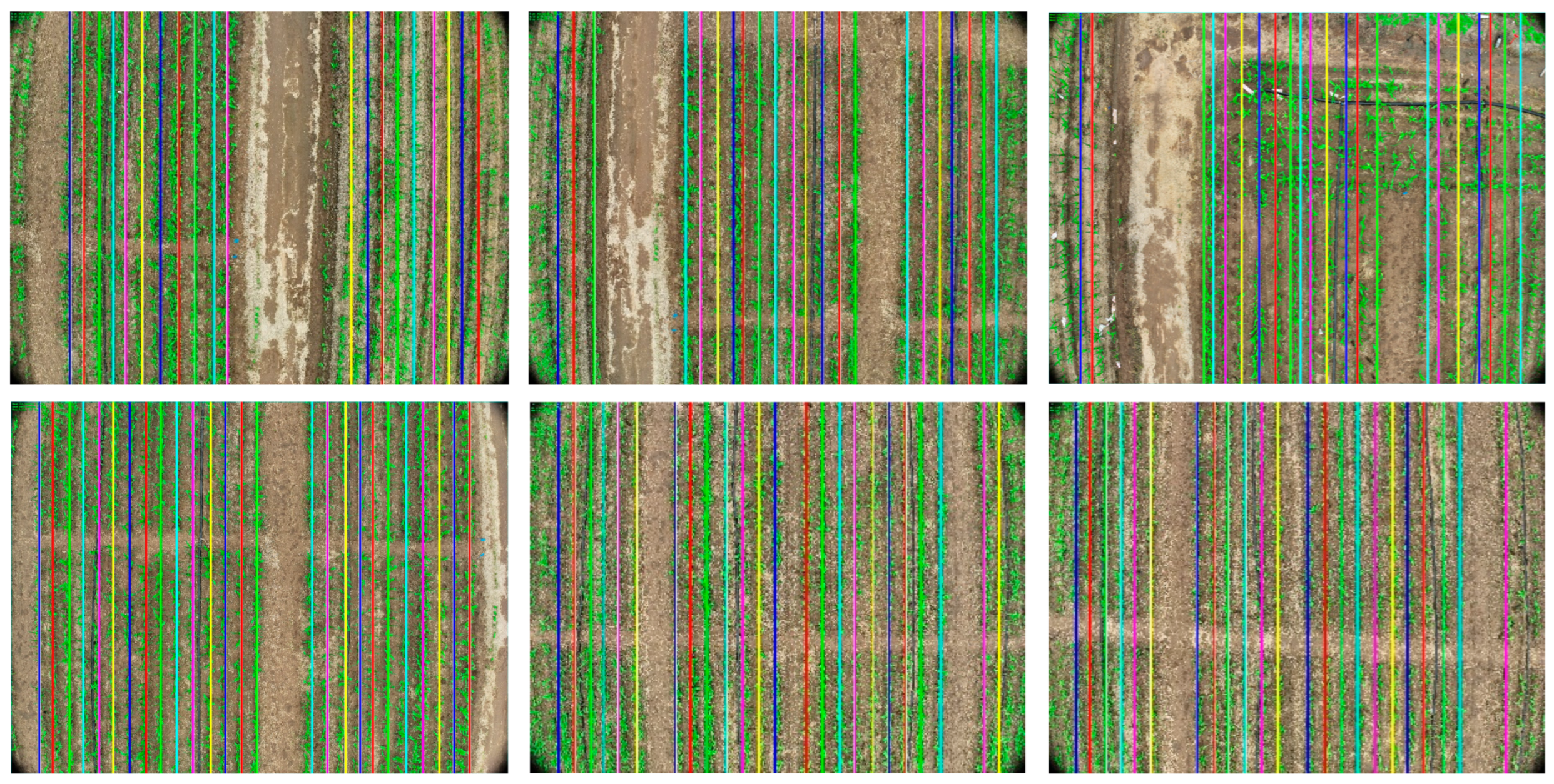
Taking partial derivatives of $J\left(\mathbf{k}\right)$ and setting them to 0, the polynomial coefficients can be solved. Substituting $\mathrm{x}$ into Equation (7) yields the fitted row curve. As shown in Figure 5, this method can simultaneously detect multiple parallel corn rows and calculate row and plant spacing parameters on each row. Different colored lines in the figure represent the detected rows, cyan rectangular boxes indicate the ROI, and the upper left corner displays measurement results, including the average row spacing, plant spacing, and tilt angle.

Figure 5. Detection results of corn rows and parameter measurement.

(c)

Agronomic Parameter Calculation

Corn row spacing is the vertical distance between the center lines of adjacent seedling rows. Based on the fitted curves, several sampling heights can be taken in the $\mathrm{Y}$ direction. If $x_{ij}$ represents the x-coordinate of the $j$th sampling point on row $i$, then the row spacing can be represented as follows:

$${\mathrm{R}\mathrm{o}\mathrm{w}\mathrm{G}\mathrm{a}\mathrm{p}}_i={\displaystyle \frac{1}{M}}{\sum }_{j=1}^M\left|x_{i+1,j}-x_{i,j}\right|$$

(9)

where $M$ is the number of sampling layers. Considering the variation in row spacing in different areas, the final result is represented by the average of all row spacings:

$$\mathrm{R}\mathrm{o}\mathrm{w}\mathrm{G}\mathrm{a}\mathrm{p}={\displaystyle \frac{1}{L-1}}{\sum }_{i=1}^{L-1}{\mathrm{R}\mathrm{o}\mathrm{w}\mathrm{G}\mathrm{a}\mathrm{p}}_i$$

(10)

Plant spacing refers to the distance between adjacent plants in the same row. Traditionally, local maximum points can reflect plant centers, but, during the seedling stage, individual plants are still difficult to accurately segment. Therefore, a cluster analysis method is adopted, using pixel density changes to mark plant intervals. Specifically, in the strip area of row $\mathrm{m}$, several vertical slices are taken at equal intervals, and the number of vegetation pixels in each slice $N_m^{\mathrm{\prime }}$ is calculated. When the difference in adjacent slice counts $\left|\Delta {\mathrm{N}}_{\mathrm{m}}^{\mathrm{\prime }}\right|$ exceeds a threshold, it is considered that a plant interval jump has occurred. The coordinates of the jump midpoint are recorded as $y_{m,i}$. Then, the average plant spacing for row $m$ is as follows:

$${\mathrm{PlantGap}}_m={\displaystyle \frac{1}{N_m-1}}{\sum }_{i=1}^{N_m-1}\left|y_{m,i+1}-y_{m,i}\right|$$

(11)

where $N_m$ is the number of plants detected in row $m$. Furthermore, the overall plant spacing in the region takes the average of plant spacings from each row:

$$\mathrm{PlantGap}={\displaystyle \frac{1}{L}}{\sum }_{m=1}^L{\mathrm{PlantGap}}_m$$

(12)

It should be noted that the above pixel distance needs to be multiplied by a scaling factor S to reflect the actual physical length. Parameter $S$ can be obtained through ground target calibration.

2.3. Agricultural Machinery Navigation and Repositioning System

Based on the aforementioned crop row detection method, an agricultural machinery navigation and repositioning system is designed to solve the problem of repositioning accuracy after agricultural machinery turns around in field operations. The system mainly includes three core modules: position memory, path planning, and overlap detection.

2.3.1. Position Memory Module

The position memory module constructs and updates a field operation map in real-time, records processed areas, and provides spatial reference for agricultural machinery. This module uses a grid map representation method with the following mathematical model:

Grid map mathematical model: Define the grid map M as a two-dimensional matrix:

$$M=\left\{m_{i,j}\right|i=1,2,...,W;j=1,2,...,H\}$$

(13)

where $W$ and $H$ represent the width and height of the map, respectively, and the state of each grid unit $m_{i,j}$ is as follows:

$$m_{i,j}=\left\{\begin{array}{ll}0,& \mathrm{unprocessed} \mathrm{area}\\ t,& \mathrm{processed} \mathrm{area},t \mathrm{is} \mathrm{timestamp}\end{array}\right.$$

(14)

GPS coordinate to grid mapping: Define the mapping function $\mathrm{f}:\left(lat,lon\right)\to \left(i,j\right)$, which maps GPS coordinates to grid coordinates:

$$\begin{gathered} i=\lfloor \left(lon-lo{n}_{min}\right)/resolution\rfloor \\ j=\lfloor \left(lat-la{t}_{min}\right)/resolution\rfloor \end{gathered}$$

(15)

where $\left(la{t}_{min},lo{n}_{min}\right)$ is the GPS coordinate of the map origin, and resolution is the resolution parameter (set to 0.05 m/pixel in this system).

Map update algorithm: When the agricultural machinery moves, the map is updated based on the current position $\left(\mathrm{l}\mathrm{a}\mathrm{t},\mathrm{l}\mathrm{o}\mathrm{n}\right)$, heading angle $\theta$, and operating width $w$:

(1)

Calculate the polygon vertices of the area covered by the agricultural machinery:

$$\mathrm{P}=\{{\mathrm{p}}_1,{\mathrm{p}}_2,{\mathrm{p}}_3,{\mathrm{p}}_4\}$$

(16)

where

$$p_1=\left(i-{\displaystyle \frac{w}{2}}\mathrm{s}\mathrm{i}\mathrm{n}\theta ,j+{\displaystyle \frac{w}{2}}\mathrm{c}\mathrm{o}\mathrm{s}\theta \right)$$

$$p_2=\left(i+{\displaystyle \frac{w}{2}}\mathrm{s}\mathrm{i}\mathrm{n}\theta ,j-{\displaystyle \frac{w}{2}}\mathrm{c}\mathrm{o}\mathrm{s}\theta \right)$$

$$p_3=\left(i+{\displaystyle \frac{w}{2}}\mathrm{s}\mathrm{i}\mathrm{n}\theta +d\mathrm{c}\mathrm{o}\mathrm{s}\theta ,j-{\displaystyle \frac{w}{2}}\mathrm{c}\mathrm{o}\mathrm{s}\theta +d\mathrm{s}\mathrm{i}\mathrm{n}\theta \right)$$

$$p_4=\left(i-{\displaystyle \frac{w}{2}}\mathrm{s}\mathrm{i}\mathrm{n}\theta +d\mathrm{c}\mathrm{o}\mathrm{s}\theta ,j+{\displaystyle \frac{w}{2}}\mathrm{c}\mathrm{o}\mathrm{s}\theta +d\mathrm{s}\mathrm{i}\mathrm{n}\theta \right)$$

and d is the coverage length in the forward direction.

(2)

Fill the polygon area grid: For each grid, $m_{i,j}$, within the polygon, update the state:

$$m_{i,j}=t_{current}$$

(17)

Overlap detection: Define the overlap function $O\left(P\right)$:

$$O\left(P\right)={\displaystyle \frac{\sum _{\left(i,j\right)\in P}\left[m_{i,j}>0\right]}{\sum _{\left(i,j\right)\in P}1}}\times 100\mathrm{\%}$$

(18)

when $O\left(P\right)>{\mathsf{\tau }}_{\mathrm{o}\mathrm{v}\mathrm{e}\mathrm{r}\mathrm{l}\mathrm{a}\mathrm{p}}$ (set to ${\mathsf{\tau }}_{\mathrm{o}\mathrm{v}\mathrm{e}\mathrm{r}\mathrm{l}\mathrm{a}\mathrm{p}}=10\mathrm{\%}$ in this system), an overlap warning is triggered.

2.3.2. Path Planning and Turn Optimization

Multi-row coverage path planning: Given $\mathrm{n}$ detected parallel crop rows $\{{\mathrm{L}}_1,{\mathrm{L}}_2,...,{\mathrm{L}}_{\mathrm{n}}\}$ and considering the operating width $\mathrm{w}$ of the agricultural machinery, calculate the optimal coverage path.

First calculate the optimal row grouping:

$$G=\lfloor w/\bar{d}\rfloor$$

(19)

where $\bar{d}$ is the average row spacing and $G$ is the number of rows covered in a single pass.

Bezier curve turning path: During the turning process from the end of row group $\mathrm{i}$ to the starting point of row group $\mathrm{i}+\mathrm{G}$, a cubic Bezier curve is used to generate a smooth turning path:

$$B\left(t\right)={\left(1-t\right)}^3{P}_0+3{\left(1-t\right)}^{2}t{P}_1+3\left(1-t\right)t^2{P}_2+t^3{P}_3,t\in \left[0,1\right]$$

(20)

where control points $P_0,P_1,P_2,P_3$ are calculated as follows: (1) $P_0$ is the endpoint of the current row group; (2) $P_3$ is the starting point of the target row group; (3) $P_1=P_0+R\cdot \overrightarrow{v_0}$, where $\overrightarrow{v_0}$ is the travel direction vector at $P_0$ and $R$ is the turning radius; (4) $P_2=P_3-R\cdot \overrightarrow{v_3}$, where $\overrightarrow{v_3}$ is the travel direction vector at $P_3$.

Adaptive sampling density control: In the turning area, the sampling point density $\rho$ is dynamically adjusted according to the curvature $\kappa$:

$$\rho \left(t\right)={\rho }_{base}\cdot \left(1+\alpha \cdot \kappa \left(t\right)\right)$$

(21)

where $\kappa \left(t\right)$ is the curvature of the Bezier curve at parameter $t$:

$$\kappa \left(t\right)={\displaystyle \frac{\left|B\mathrm{\prime }\left(t\right)\times B″\left(t\right)\right|}{{\left|B\mathrm{\prime }\left(t\right)\right|}^3}}$$

${\rho }_{\mathrm{b}\mathrm{a}\mathrm{s}\mathrm{e}}$ is the base sampling density, and $\alpha$ is the density adjustment coefficient (this system applies 5.0).

2.3.3. Overlap Detection and Correction

Adjacent row boundary distance calculation: During travel, the distance from the current position to the nearest processed area boundary is calculated in real-time:

$$d_{border}\left(i,j\right)=\underset{\left(i\mathrm{\prime },j\mathrm{\prime }\right)\in \partial M_1}{\mathrm{m}\mathrm{i}\mathrm{n}}\sqrt{{\left(i-i\mathrm{\prime }\right)}^2+{\left(j-j\mathrm{\prime }\right)}^2}\cdot resolution$$

(22)

where $\partial M_1$ represents the set of boundary points of the processed area.

Lateral position adaptive adjustment: When potential overlap is detected ($d_{border}<d_{threshold}$), the lateral position adjustment amount is calculated as follows:

$$\Delta x=K_p\left(d_{target}-d_{border}\right)+K_d{\displaystyle \frac{d}{dt}}\left(d_{target}-d_{border}\right)$$

(23)

where $d_{target}$ is the target boundary distance, and $K_p$ and $K_d$ are the proportional and differential control coefficients, respectively (set to $K_p=0.7$, $K_d=0.2$ in this system).

Row spacing trend prediction: Based on the detected row spacing data, the weighted moving average is used to predict the next row position:

$${\widehat{d}}_{next}={\displaystyle \frac{\sum _{i=1}^k{w}_i\cdot d_{n-i+1}}{\sum _{i=1}^k{w}_i}}$$

(24)

where $w_i={\mathrm{e}}^{-\lambda \left(i-1\right)}$ is the exponentially decaying weight ($\lambda =0.3$ in this system) and $d_{n-i+1}$ is the $\mathrm{i}$-th last-observed row spacing.

Path feedforward control: Based on the predicted row spacing, the agricultural machinery path is corrected to the following:

$$x_{corrected}=x_{planned}+\beta \cdot \left({\widehat{d}}_{next}-\bar{d}\right)$$

(25)

where $\beta$ is the feedforward gain coefficient ($\beta =0.5$ in this system), used to balance the tracking accuracy and system stability.

Through the above mathematical models and algorithms, the system can effectively solve the problem of repositioning accuracy when agricultural machinery makes U turns, theoretically reducing missed harvesting and overlap rates and improving operation efficiency.

2.4. Evaluation Metrics

2.4.1. Data and Evaluation Indicators

To verify the effectiveness of this method, typical images from different plots, row numbers, and weed interference scenarios in the test area are selected, totaling 60 images covering 6–8 corn rows. Meanwhile, manual annotation is performed on the original images to obtain pixel-level standard row ground truth. Referring to reference [29], precision, recall, and F1 score metrics were used to quantitatively evaluate the pixel-level accuracy of row detection:

$$\mathrm{p}\mathrm{r}\mathrm{e}\mathrm{c}\mathrm{i}\mathrm{s}\mathrm{i}\mathrm{o}\mathrm{n}={\displaystyle \frac{\mathrm{T}\mathrm{P}}{\mathrm{T}\mathrm{P}+\mathrm{F}\mathrm{P}}}$$

$$\mathrm{r}\mathrm{e}\mathrm{c}\mathrm{a}\mathrm{l}\mathrm{l}={\displaystyle \frac{\mathrm{T}\mathrm{P}}{\mathrm{T}\mathrm{P}+\mathrm{F}\mathrm{N}}}$$

(26)

$$F1={\displaystyle \frac{2\cdot \mathrm{p}\mathrm{r}\mathrm{e}\mathrm{c}\mathrm{i}\mathrm{s}\mathrm{i}\mathrm{o}\mathrm{n}\cdot \mathrm{r}\mathrm{e}\mathrm{c}\mathrm{a}\mathrm{l}\mathrm{l}}{\mathrm{p}\mathrm{r}\mathrm{e}\mathrm{c}\mathrm{i}\mathrm{s}\mathrm{i}\mathrm{o}\mathrm{n}+\mathrm{r}\mathrm{e}\mathrm{c}\mathrm{a}\mathrm{l}\mathrm{l}}}$$

where TP (true positive) is the number of pixels detected as rows and annotated as rows, FP (false positive) is the number of pixels detected as rows but annotated as background, and FN (false negative) is the number of pixels detected as background but annotated as rows. These metrics take values in the interval [0, 1], with values closer to 1 indicating better detection results. For the measurement error of agronomic parameters, the Mean Absolute Percentage Error (MAPE) metric is used:

$$\mathrm{M}\mathrm{A}\mathrm{P}\mathrm{E}={\displaystyle \frac{100\mathrm{\%}}{N}}{\sum }_{i=1}^N{\displaystyle \frac{\left|G_i-P_i\right|}{\left|G_i\right|}}$$

(27)

where $G_i$ is the manually measured row spacing or plant spacing of region $i$, $P_i$ is the algorithm measured value, and $N$ is the total number of regions. MAPE reflects the level of relative error, with lower values indicating more accurate measurements.

All indicators are calculated as a mean, standard deviation, and 95% confidence interval. Paired t-test are used to compare the differences between different methods, with a significance level set at p < 0.05.

2.4.2. Parameter Settings

ROI extraction parameters: The upper boundary relative height is set to 0.10; left and right boundaries are indented by 10%.

Row segmentation parameters: The green component thresholds are $H_{\mathrm{m}\mathrm{i}\mathrm{n}}=35$ and $H_{\mathrm{m}\mathrm{a}\mathrm{x}}=90$, and the opening and closing operation kernel sizes are both $5\times 5$.

Row fitting parameters: Peak search height $=0.25 H$, minimum peak width $=0.01 W$, minimum peak distance $=0.10 W$, sliding window radius $R=25$, minimum vegetation pixel count in window $N_{\mathrm{m}\mathrm{i}\mathrm{n}}=15$, and vertical sliding step is 1/6 of the window height. Quadratic polynomial fitting uses the least squares method with 30 iterations.

Row spacing and plant spacing calculation parameters: For row spacing sampling layers, $M=5$, plant spacing slice count is taken as 1/20 of the row length, and the density difference threshold is 1/3 of the peak value. The pixel scale factor is $S=0.820$ cm/pixel.

3. Experimental Results and Analysis

Table 1 shows the quantitative evaluation results of downlink detection in different experimental scenarios. It can be seen that the algorithm has achieved a high level of overall accuracy, recall, and F1 score, with average values of 93.8%, 91.5%, and 0.925, respectively. Especially in the six-row area, the best results were achieved (F1 = 0.943), mainly due to the wider row spacing and clearer plant distribution. The high precision indicates that most of the detected seedling belt pixels are correct, while recall reflects the integrity of the overall seedling area depiction. The results of different row spacing combinations in the table indicate that the accuracy decreased when the number of rows increased, and the F1 score of the eight-row region dropped to 0.907. This is mainly because denser seedling belts are more prone to adhesion, which interferes with segmentation and fitting. Under extremely dense planting conditions (>eight rows, row spacing <50 cm), peak merging may occur, leading to an insufficient detection, which is a known limitation of the histogram method.

Table 1. Pixel-level accuracy of downlink detection under different scenarios (mean ± standard deviation, n = 60).

Scenario Type	Precision (%)	Recall (%)	F1 Score (%)
Six-row region	95.2 ± 1.8	93.4 ± 2.1	94.3 ± 1.5
Seven-row region	94.1 ± 2.3	91.8 ± 1.9	92.9 ± 1.8
Eight-row region	92.1 ± 2.7	89.3 ± 2.6	90.7 ± 2.1
Light weeds	94.8 ± 1.6	92.6 ± 1.7	93.7 ± 1.4
Medium weeds	93.5 ± 2.2	90.8 ± 2.4	92.1 ± 1.9
Heavy weeds	92.9 ± 2.8	90.1 ± 2.9	91.5 ± 2.3
Average	93.8 ± 2.1	91.5 ± 1.8	92.5 ± 1.8

Note: p value compared to the reference group (six-row area or medium weeds).

In addition, although the weed problem subtly affected the recall rate, the detection performance has maintained a high level through morphological operations such as opening and closing, and even under severe weed interference; the F1 score has reached 0.915. Overall, this method demonstrates a strong adaptability to different seedling stages, row plant configurations, and weed conditions.

Table 2 shows the MAPE indicators for row spacing and plant spacing measurements in different areas. The six-row area shows the best measurement results, with a row spacing MAPE of only 1.83%, which is an actual error of only about 1.1 cm compared to the standard 60 cm design row spacing. The average row spacing errors for the six-, seven-, and eight-row areas are 1.83%, 2.35%, and 2.92%, respectively, generally better than ±2.5 cm. The plant spacing MAPEs are 2.46%, 2.85%, and 3.31%, respectively, corresponding to physical distances of about 0.62 cm, 0.71 cm, and 0.83 cm. Considering that the image resolution is 0.82 cm/pixel, a row spacing measurement error of ±2.5 cm is completely acceptable in practical agricultural applications.

Table 2. Row and plant spacing measurement errors in different regions (n = 20/region).

Region Type	Average Row Spacing (cm)	Row Spacing MAPE (%)	Average Plant Spacing (cm)	Plant Spacing MAPE (%)
Six-row region	60.2 ± 1.3	1.83 ± 0.42	25.62 ± 0.20	2.46 ± 0.8
Seven-row region	59.8 ± 1.5	2.35 ± 0.38	25.71 ± 0.23	2.85 ± 0.9
Eight-row region	59.5 ± 1.7	2.92 ± 0.46	25.83 ± 0.28	3.31 ± 1.1
Average	59.8 ± 1.5	2.37 ± 0.42	25.72 ± 0.23	2.87 ± 0.9

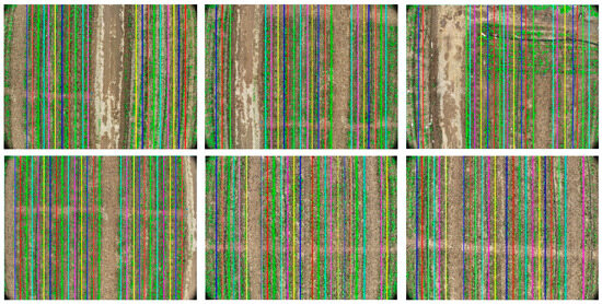
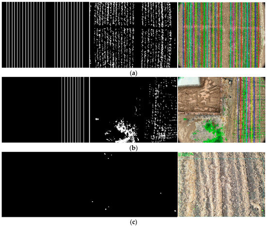
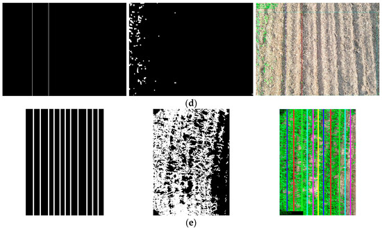
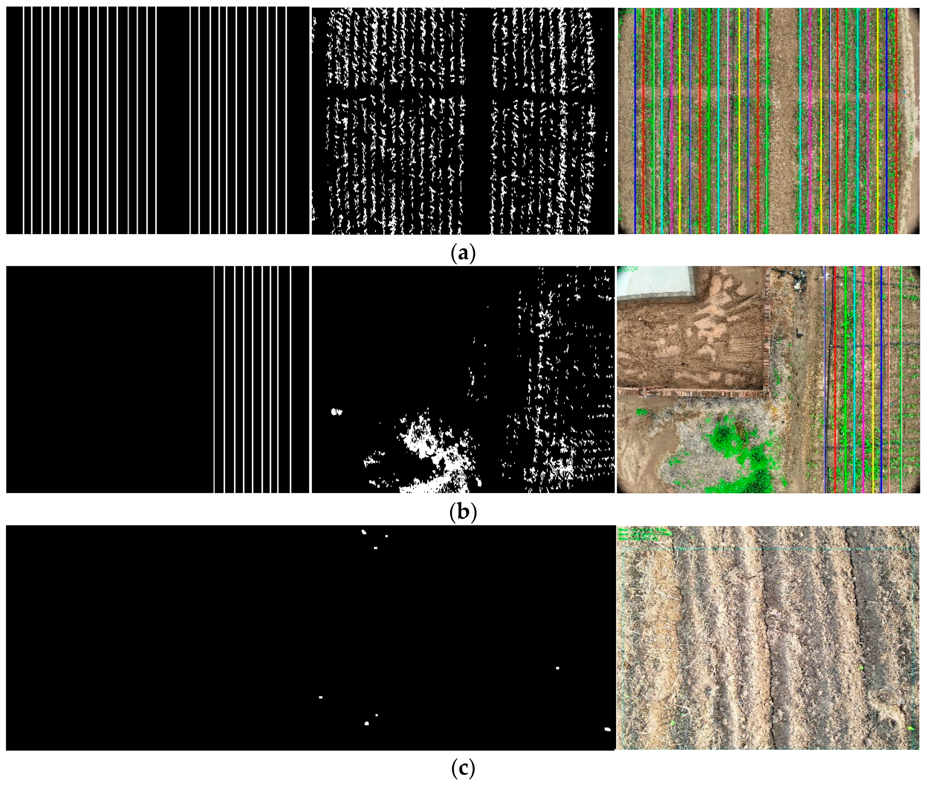
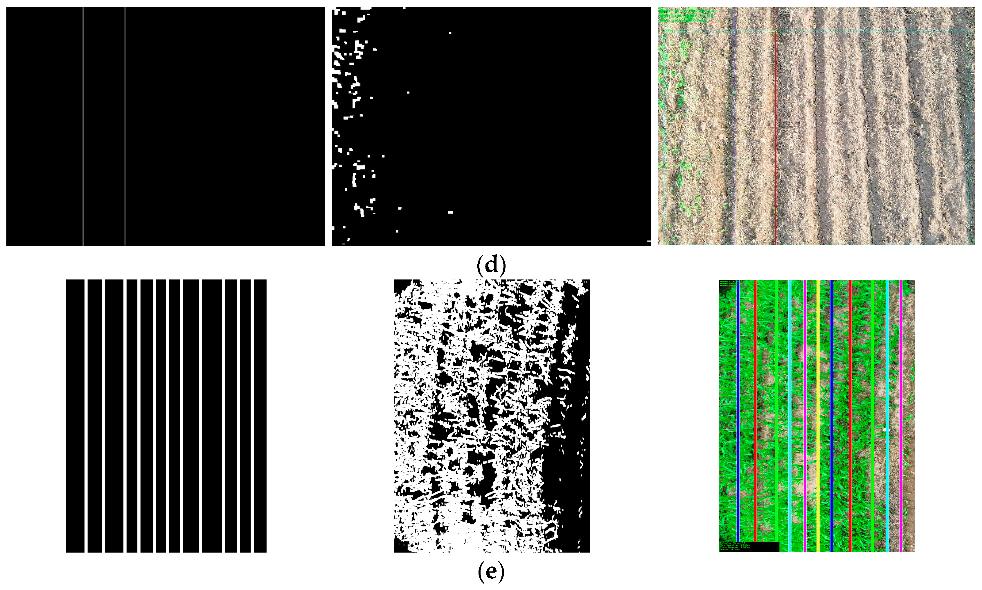
Figure 6 shows the row detection results under different scenarios. From the figure, it can be observed that, (a) under ideal growth conditions, the algorithm can precisely identify clear and regular rows, with detection results highly matching the actual rows; (b) even in cases of irregular plant distribution and uneven plant spacing, the algorithm can still accurately locate and fit complete row trajectories; (c) for areas with no seedlings or extremely sparse plants, the algorithm intelligently avoids false detection and does not output detection results, showing a strong discrimination ability; (d) in complex environments with weed interference, the algorithm maintains a stable detection performance, effectively distinguishing crops from weeds and accurately identifying real crop rows; (e) for special cases of row adhesion, a good detection performance is still persevered. These results fully demonstrate the adaptability and reliability of the method in different field scenarios, meeting the requirements for row detection in actual agricultural production.

Figure 6. Detection results of corn rows under different scenarios. (a) Accurate detection under ideal conditions; (b) robust detection under irregular plant spacing conditions and interference; (c) accurate discrimination of areas without seedlings; (d) robust recognition under weed interference; (e) identification with row adhesion characteristics.

Figure 6 demonstrates the detection capability of the algorithm in various complex scenarios. (a) shows a precise detection under ideal conditions; (b) demonstrates a robustness in irregular plant distribution; (c) proves the algorithm’s accurate judgment for areas without seedlings; (d) shows the stable performance under weed interference; and (e) indicates row adhesion identification.

3.1. Comparison of Corn Row Detection Effects of Different Algorithms in the Same Scenario

To comprehensively evaluate the performance of the method in this paper, other mainstream crop row detection algorithms are compared.

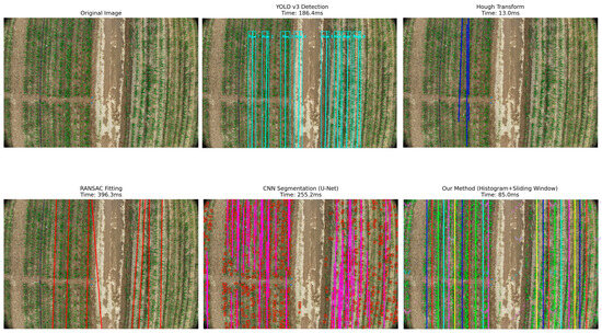
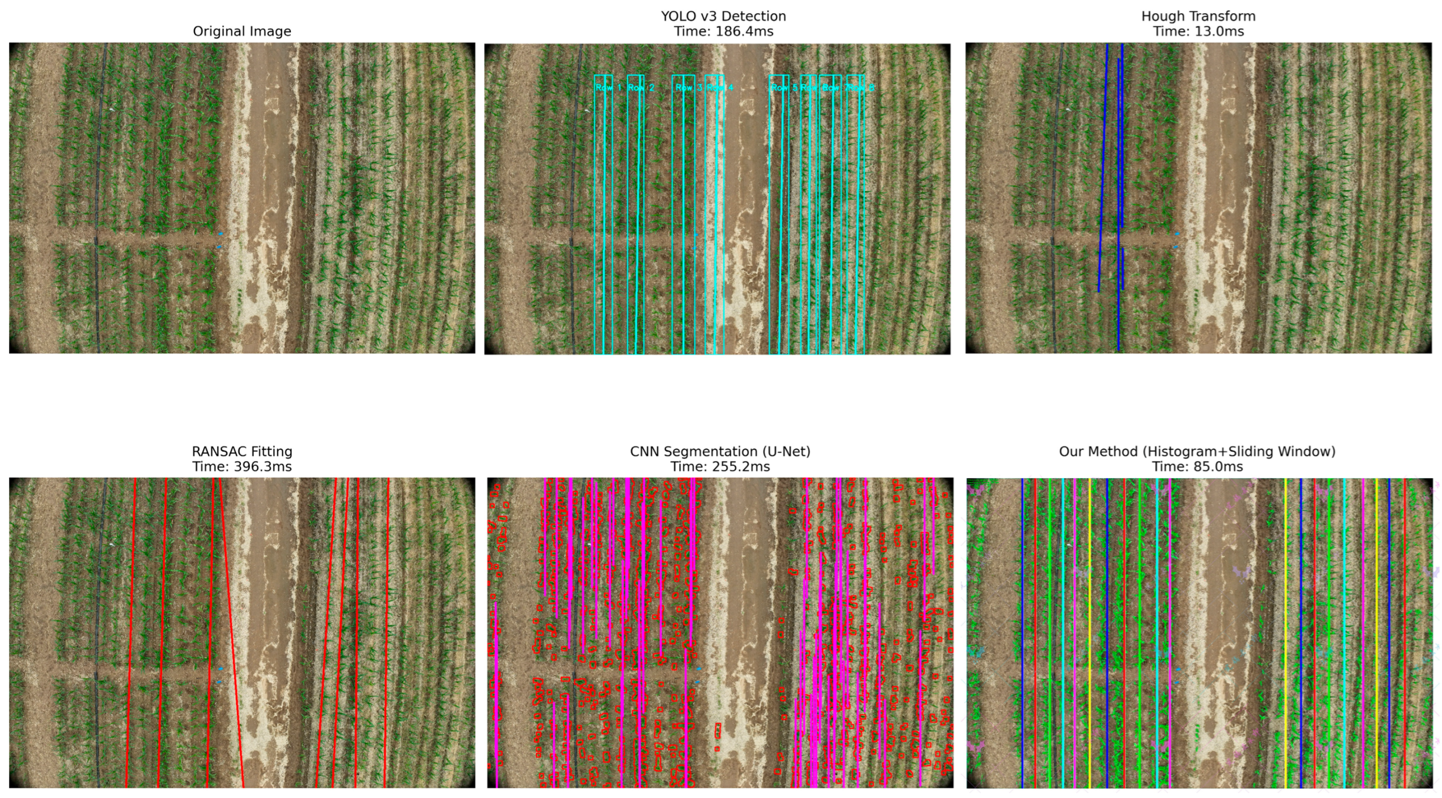
Figure 7 visually shows the comparison of corn row detection effects of five different algorithms in the same farmland scenario. The following analysis can be drawn from visual results and performance data:

Figure 7. Detection comparison among different algorithms under same scenario.

The last result in Figure 7 is the method proposed in this paper (histogram peak + sliding window), which demonstrates an excellent detection capability, successfully identifying almost all corn rows in the image, clearly marking them with multiple colors. The row lines are neatly arranged with uniform spacing, and the entire vegetation area can be accurately covered, showing a good adaptability to complex farmland environments. The processing time is 85.0 ms, achieving a good balance between accuracy and efficiency.

In contrast, the Hough transform method, although the fastest (only 13.0 ms), only detects a few blue straight lines, with a serious missed detection, unable to meet the actual application needs. This indicates that simple linear detection methods have difficulty coping with complex field environments.

The RANSAC fitting method detects red row lines with obvious curved characteristics, showing a certain adaptability, but the lines are not regular enough, and there are offset phenomena in some areas. Its processing time is as high as 396.3 ms, with low computational efficiency, making it difficult to meet real-time processing requirements.

Among deep learning methods, CNN semantic segmentation (U-Net) generates dense pink and red row lines with a high coverage, but with line breakage and local disorder, especially in weed interference areas. The processing time is 255.2 ms, with a high computational overhead. The YOLO v3 detection method accurately marks each row with neat cyan lines and rectangular boxes, and provides row number identifications, with clear visual effects, but the processing time is 186.4 ms, also requiring high computational resources.

In order to quantitatively evaluate the comprehensive performance of each algorithm, Table 3 provides a detailed comparison from multiple dimensions such as detection accuracy, computational efficiency, memory usage, and hardware requirements

Table 3. Comprehensive comparison of performance of different algorithms (n = 30).

Algorithm	Precision (%)	Recall (%)	F1 Score (%)	Processing Time (ms)	RAM Usage (MB)	Hardware
Hough Transformation	68.3 ± 5.2	71.2 ± 4.8	69.7 ± 4.8	13.0 ± 2.1	128	CPU
RANSAC Fitting	82.7 ± 3.6	79.4 ± 4.1	80.9 ± 3.5	396.3 ± 18.7	256	CPU
U-Net	91.2 ± 2.4	88.6 ± 2.7	89.9 ± 2.3	255.2 + 12.3	4096	GPU
YOLO v3	90.8 ± 2.6	89.3 ± 2.5	90.0 ± 2.4	186.4 ± 9.8	2048	GPU
Proposed Method	93.8 ± 2.1	91.5 ± 1.8	92.5 ± 1.8	85.0 ± 4.3	512	CPU

Note: Hardware platform: Intel Core i7-9750H CPU (2.60 GHz), 16 GB RAM, without GPU acceleration.

The quantitative comparison results revealed several key findings:

Traditional method analysis: Although Hough transform is extremely fast (13.0 ms), it has serious limitations in handling curved lines and complex scenes (F1 = 0.697), and its accuracy is far below practical requirements. The RANSAC fitting method has improved the adaptability of curve patterns (F1 = 0.809), but it requires a long computation time (396.3 ms), which makes it difficult to meet real-time processing requirements.

Analysis of deep learning methods: U-Net (F1 = 0.899) and YOLO v3 (F1 = 0.900) have both achieved strong detection accuracy, but require a large amount of computing resources (more than 4 GB memory) and a longer processing time (186–255 ms). In addition, deep learning methods also face challenges such as difficulty in sample annotation, high training costs, and limited model generalization ability.

The histogram peak detection combined with sliding window method proposed in this article achieves a competitive detection accuracy (F1 = 0.925), while maintaining excellent computational efficiency (85 ms, only requiring CPU). The memory usage is only 512 MB, far below the several GB level requirements of deep learning methods, making it particularly suitable for resource-constrained embedded systems. The processing speed can achieve real-time operation of about 12 frames per second, meeting the needs of autonomous navigation applications. More importantly, this method requires almost no training data, avoiding the annotation cost and generalization problems of deep learning methods and facilitating the rapid deployment to different regions and crop varieties.

3.2. Repositioning Accuracy Evaluation

To verify the effect of the system in solving the problem of agricultural machinery repositioning accuracy, extended experiments are conducted in the same test area. The results show that, after system optimization, the repositioning accuracy of agricultural machinery after turning around is significantly improved.

As shown in Table 4, under the traditional RTK navigation method, the lateral positioning error of agricultural machinery after turning around is ±8.2 cm on average, with a maximum of 15.3 cm. After adopting this system, the lateral positioning error is reduced to an average of ±2.8 cm, with a maximum error less than 4.9 cm. This improvement in accuracy effectively reduces operation overlap and missed harvesting, especially in multiple round trips in the same field.

Table 4. Comparison of repositioning accuracy of different navigation systems.

Navigation Method	Averaged Lateral Deviation (cm)	Max Lateral Deviation (cm)	Omission Rate (%)	Overlap Rate (%)
Typical RTK Navigation	8.2 ± 1.9	15.3	3.6 ± 0.8	7.2 ± 1.1
Proposed Method (Row Detection + Map)	2.8 ± 0.6	4.9	0.8 ± 0.3	1.5 ± 0.4
Proposed Method (High Speed Mode) *	3.1 ± 0.7	5.2	1.0 ± 0.3	1.8 ± 0.5

* Note: The high-speed operation test refers to the performance of agricultural machinery running at a speed of 2.0 m/s, demonstrating the robustness of the method proposed in this paper at different operating speeds.

In addition, the system maintains a stable positioning accuracy at different working speeds. In the speed range of 0.5 m/s to 2.0 m/s, the positioning accuracy variation is less than 0.5 cm, demonstrating the real-time performance and robustness of the algorithm. This system reduces the overlap rate in agricultural machinery operations from 7.2% with traditional methods to 1.5%, and the missed harvesting rate (omission rate) from 3.6% to 0.8%, providing reliable technical support for precision agriculture.

3.3. Applicability Verification for Different Growth Stages

Corn exhibits significantly different morphological characteristics at different growth stages, from a low and sparse canopy in the three-leaf stage to a closed canopy in the seven-leaf stage. Changes in plant height, leaf number, and coverage can all affect the difficulty and accuracy of line detection. To verify the applicability and robustness of our method in different growth stages, we conducted supplementary tests in three key growth stages. Table 5 shows the detection performance indicators for different growth stages.

Table 5. Detection performance across different growth stages.

Stage	Seedling Height (cm)	Number of Leaves	F1 Score	Spacing Error (cm)	Compatibility
Three-leaf	15–30	3–4	0.925 ± 0.018	±2.3	Excellent
Five-leaf	35–50	5–6	0.912 ± 0.023	±2.8	Good
Seven-leaf	60–80	7–8	0.887 ± 0.031	±3.6	Acceptable

Experimental results demonstrate the growth stage adaptability characteristics of the proposed method:

At the three-leaf stage, maize plants are relatively short (15–30 cm), with clearly distinguishable row lines and obvious plant spacing. The proposed method achieves an optimal detection performance (F1 = 0.925, row spacing error ±2.3 cm). This stage corresponds to a critical period for field management operations, such as early-stage directional spraying and topdressing. High-precision row line detection can provide a reliable navigation basis for these operations, enabling precise applications.

Upon reaching the five-leaf stage, the plant height increases to 35–50 cm, the number of leaves increases, and the canopy begins to approach but has not yet closed. The detection performance remains at a good level (F1 = 0.912), with a slight increase in the row spacing measurement error (±2.8 cm), which is still within the acceptable range for precision agriculture applications. The detection accuracy at this stage is sufficient to support mid-term plant protection operations and variable-rate fertilization management measures.

By the seven-leaf stage, the plant height reaches 60–80 cm, the canopy begins to close, and leaf occlusion and overlap become significantly more pronounced. Although detection difficulty increases, the proposed method still achieves an acceptable performance (F1 = 0.887), albeit with an increased measurement uncertainty (row spacing error ±3.6 cm). Increased plant height and leaf occlusion introduce more segmentation uncertainty, but the method remains practical for operations with general accuracy requirements, such as inter-row weeding in later stages.

The comprehensive analysis indicates that the proposed method is most suitable for applications in the early- to mid-growth stages (three-leaf to five-leaf stages), which precisely correspond to key agricultural operation periods requiring high-precision positioning, such as precise pesticide application at the seedling stage, early topdressing, and mechanical inter-row weeding. Although accuracy declines in later stages, the method remains usable for operations with relatively lower precision requirements. This adaptability characteristic aligns well with the actual needs of agricultural production, validating the practicality of the method.

3.4. Validation of Water-Saving Effects

The ultimate goal of precise crop row detection is to achieve targeted application, thereby conserving resources—particularly water resources, which are crucial for sustainable agriculture. To quantify the actual benefits of the precise spraying system proposed in this study, a comparative field experiment was conducted on a 10 mu (approximately 0.67 hectares) test field with three replicates. The experiment systematically compared traditional uniform spraying and precise spraying based on the row detection system.

Table 6 presents a comparison of resource consumption and agronomic outcomes between the two spraying methods:

Table 6. Comparison of precision spraying and conventional spraying (10-acre experimental field, three bouts).

Metrics	Typical Average Spray	Precision Spray	Conservation Ratio (%)	p Value
Water usage (L/acre)	187.3 ± 8.6	147.2 ± 6.3	21.4 ± 2.8	<0.001
Pesticide usage (kg/acre)	2.84 ± 0.13	2.17 ± 0.09	23.6 ± 3.1	<0.001
Operation time (min/acre)	12.5 ± 1.1	11.8 ± 0.9	5.6 ± 1.8	0.042
Crop yield (kg/acre) *	628.7 ± 31.2	634.5 ± 29.8	+0.9 ± 1.2	0.386

* Note: Yield measurement data at harvest stage.

The field trial results demonstrated that precision spraying significantly conserved resources without compromising crop productivity. The water usage for precision spraying was reduced by 21.4%, from 187.3 L per mu to 147.2 L per mu, equivalent to saving approximately 40 L per mu per application. Based on three to five plant protection operations per season, this translates to a water savings of 12 to 20 tons for 100 mu of farmland, which is of great significance in water-scarce regions. The difference was statistically significant (p < 0.001). Pesticide usage decreased by 23.6%, from 2.84 kg per mu to 2.17 kg per mu, reflecting the system’s precise crop row identification and targeting capabilities. This not only reduced input costs but also minimized environmental pollution and pesticide residue risks, contributing to the health of the farmland ecosystem. The operational time was shortened by 5.6% (p = 0.042), attributed to optimized travel paths and a reduced redundant coverage, thereby lowering the fuel consumption and operational costs. In terms of yield, no significant difference was observed between the two methods (p = 0.386), validating that precision spraying achieves a reduction in input without compromising output. Overall calculations indicate that, for 100 mu of farmland per season, the cost savings amount to approximately 1400 to 2000 RMB, alongside reduced pesticide runoff, water and energy conservation, and lower greenhouse gas emissions.

4. Discussion

The method proposed in this study demonstrates significant advantages in corn row identification and agricultural machinery navigation. Firstly, the method exhibits a high computational efficiency, with an average processing time of 85 ms, which is 2–4 times faster than the existing deep learning methods (186–342 ms). Furthermore, it can run using only a CPU, eliminating the need for expensive GPU hardware. This holds considerable importance for embedded deployment and large-scale agricultural applications. Simultaneously, the method shows a good robustness under varying lighting conditions (52,300–78,600 lux) and weed densities. Even under heavy weed interference, it can achieve an F1 score of 0.925, indicating a strong anti-interference capability. Compared to deep learning methods, this approach does not require large amounts of training data, avoiding the dependency on thousands of annotated images. Moreover, its algorithmic principles are clear, and its parameters are interpretable, facilitating understanding and debugging by agricultural technicians, thereby offering a higher practicality in real-world applications.

However, this method still has some limitations. As corn grows and leaves gradually overlap, the detection accuracy decreases after the seven-leaf stage. This suggests that future work could incorporate multispectral or depth information to further improve performance. Additionally, the current method assumes a relatively flat farmland terrain; under sloped conditions, additional terrain correction is needed. Furthermore, while the method is optimized for corn and can be applicable to crops with regular row spacing and distinct leaf color differences, such as wheat and soybeans, it might require parameter adjustments or integration with deep learning methods for crops where the leaf color has a low contrast with the background (e.g., sunflowers).

Based on the current achievements, future research can be improved in several aspects. Firstly, multi-modal data fusion, incorporating information beyond RGB/visible light—such as multispectral data and LiDAR—could enhance the detection accuracy under complex conditions. Secondly, developing-edge computing hardware acceleration solutions based on FPGA or ARM could further reduce system power consumption and cost. Furthermore, leveraging GPU acceleration and embedded implementation could enable real-time perception for autonomous drone navigation and the development of lightweight agricultural machinery navigation control systems, achieving a seamless integration between drone detection results and farm machinery operations. Simultaneously, establishing a distributed operation system to enable collaborative work and information sharing among multiple agricultural machines would further enhance the system’s application value in large-scale precision agriculture.

5. Conclusions

An automated method for measuring row spacing and plant spacing in maize at the seedling stage based on UAV imagery is proposed. The method begins by extracting field vegetation regions using color segmentation and mathematical morphology. A perspective transformation is then applied to obtain an accurate top-down view, and histogram analysis is used to roughly locate the row centers. On this basis, a sliding window search is employed to fit parallel crop row curves in a top-down manner. Finally, the average row spacing (RowGap) and plant spacing (PlantGap) parameters are estimated based on inter-row intervals and pixel density distribution within plant bands. The experiments demonstrate that the method adapts to different growth stages, row numbers (6–8 rows), and weed density conditions, achieving a row detection precision of 93.8%, a recall of 91.5%, and an F1 score of 0.925; the row spacing measurement error is within ±2.5 cm, and the plant spacing error is less than ±3.0 cm, providing a reliable reference for optimizing maize planting density; the perspective transformation and multi-row sliding window strategy effectively mitigate the impact of oblique shooting and the local deformation of plant bands, making it suitable for complex field environments; the field mapping and navigation approach based on crop row detection effectively addresses the repositioning accuracy issue after agricultural machinery U-turns, reducing the operational overlap rate from 7.2% in conventional methods to 1.5% and the miss rate from 3.6% to 0.8%, offering robust technical support for precision agriculture. The field comparative validation shows that the system achieves 21.4% water savings and a 23.6% pesticide reduction. With no significant change in yield (p = 0.386), it saves 1400–2000 RMB per season for a 100 mu field while reducing pollution. The method can be applied to crops with regular row spacing and significant differences in leaf color, such as wheat and soybeans, but, for crops with a low contrast between the leaf color and background (such as sunflowers), additional parameter adjustments or deep learning methods may be required.

The method is lightweight and efficient, requiring only CPU operation with a memory footprint of 500–600 MB and a processing speed of 85 ms per frame (approximately 12 fps). It does not rely on large-scale annotated data and possesses a cross-regional generalization capability, making it suitable for resource-constrained environments and large-scale deployment. Perspective transformation and the multi-row sliding window effectively suppress the effects of tilt and deformation, adapting to complex field conditions. The method performs optimally at the 3–5 leaf stage (F1 ≥ 0.912), with a slight decline after the 7-leaf stage due to canopy occlusion (F1 = 0.887, row spacing error ±3.6 cm), while still meeting general operational accuracy requirements. In the future, GPU acceleration and embedded implementation should be used to achieve the autonomous navigation and real-time perception of drones, and a lightweight agricultural machinery navigation control system should be developed to achieve seamless integration between drone detection results and agricultural machinery operations.

References

- Macpherson, J.; Rosman, A.; Helming, K.; Burkhard, B. A participatory impact assessment of digital agriculture: A Bayesian network-based case study in Germany. Agric. Syst. 2025, 224, 104222. [Google Scholar] [CrossRef] [Scilit]
- Dwivedi, S.; Sherly, M.A. Multivariate assessment of digital agriculture and irrigation potential: Application to India. Agric. Syst. 2025, 227, 104328. [Google Scholar] [CrossRef] [Scilit]
- Grand View Research. Precision Farming Market Size, Share & Trends Analysis Report 2025–2030; Grand View Research: San Francisco, CA, USA, 2024; Available online: https://www.grandviewresearch.com/industry-analysis/precision-farming-market (accessed on 2 November 2025).
- Liu, C.; Lin, H.; Li, Y.; Gong, L.; Miao, Z. Analysis on status and development trend of intelligent control technology for agricultural equipment. Trans. CSAM 2020, 51, 1–18. [Google Scholar] [CrossRef]
- Zheng, H.; Zhou, X.; He, J.; Yao, X.; Cheng, T.; Zhu, Y.; Cao, W.; Tian, Y. Early season detection of rice plants using RGB, NIR-GB and multispectral images from UAV. Comput. Electron. Agric. 2020, 169, 105223. [Google Scholar] [CrossRef] [Scilit]
- Khan, M.N.; Rahi, A.; Rajendran, V.P.; Al Hasan, M.; Anwar, S. Real-time crop row detection using computer vision: Application in agricultural robots. Front. Artif. Intell. 2024, 7, 1435686. [Google Scholar] [CrossRef] [Scilit]
- Shkanaev, A.Y.; Krokhina, D.A.; Polevoy, D.V.; Panchenko, A.V.; Sholomov, D.L.; Sadekov, R.N. Analysis of straw row in the image to control the trajectory of the agricultural combine harvester. In Proceedings of the Tenth International Conference on Machine Vision, Vienna, Austria, 13–15 November 2017; Volume 10774, pp. 19–28. [Google Scholar] [CrossRef] [Scilit]
- Silva, R.; Ribeiro, A.; Aguiar, A.S.; Santos, F.N.; Sousa, A.J. Deep learning-based crop row detection for infield navigation of agri-robots. J. Field Robot. 2024, 41, 2299–2321. [Google Scholar] [CrossRef] [Scilit]
- U.S. Geological Survey. Pesticides and Water Quality; USGS: Reston, VA, USA, 2024. Available online: https://www.usgs.gov/mission-areas/water-resources/science/pesticides-and-water-quality (accessed on 27 February 2024).
- Rad, S.M.; Ray, A.K.; Barghi, S. Water pollution and agriculture pesticide. Clean Technol. 2022, 4, 1088–1102. [Google Scholar] [CrossRef] [Scilit]
- Ronchetti, G.; Mayer, A.; Facchi, A.; Ortuani, B.; Sona, G. Crop row detection through UAV surveys to optimize on-farm irrigation management. Remote Sens. 2020, 12, 1967. [Google Scholar] [CrossRef] [Scilit]
- Rabab, S.; Badenhorst, P.; Chen, Y.-P.P.; Daetwyler, H.D. A template-free machine vision-based crop row detection algorithm. Precis. Agric. 2020, 22, 124–153. [Google Scholar] [CrossRef] [Scilit]
- Adhikari, S.P.; Kim, G.; Kim, H. Deep neural network-based system for autonomous navigation in paddy field. IEEE Access 2020, 8, 71272–71278. [Google Scholar] [CrossRef] [Scilit]
- Tsouros, D.C.; Bibi, S.; Sarigiannidis, P.G. A review on UAV-based applications for precision agriculture. Information 2019, 10, 349. [Google Scholar] [CrossRef] [Scilit]
- Fortune Business Insights. Agriculture Drones Market Report 2024–2032. Pune, India, 2024. Available online: https://www.fortunebusinessinsights.com/agriculture-drones-market-102589 (accessed on 3 November 2025).
- Grand View Research. U.S. Agriculture Drone Market Report 2025–2030; Grand View Research: San Francisco, CA, USA, 2024. [Google Scholar]
- United Nations Department of Economic and Social Affairs. World Population Prospects 2024; UN DESA: New York, NY, USA, 2024; Available online: https://population.un.org/wpp/ (accessed on 30 July 2024).
- Global Market Insights. Precision Farming Market Growth Report 2025–2034. Selbyville, DE, USA, 2024. Available online: https://www.gminsights.com/industry-analysis/precision-farming-market (accessed on 21 January 2025).
- Yang, Y.; Zhou, Y.; Yue, X.; Zhang, G.; Wen, X.; Ma, B.; Xu, L.; Chen, L. Real-time detection of crop rows in maize fields based on autonomous extraction of ROI. Expert Syst. Appl. 2023, 213, 118826. [Google Scholar] [CrossRef] [Scilit]
- Li, X.; Su, J.; Yue, Z.; Wang, S.; Duan, F.; Hua, J. Vision-based navigation line extraction by combining crop row detection and RANSAC algorithm. In Proceedings of the 2022 IEEE International Conference on Mechatronics and Automation (ICMA), Guilin, China, 7–9 August 2022; pp. 1097–1102. [Google Scholar] [CrossRef] [Scilit]
- Gong, L.; Wang, C.; Du, X.; Mao, P.; Yao, L. Improving the maize crop row navigation line recognition method of YOLOX. Front. Plant Sci. 2024, 15, 1338228. [Google Scholar] [CrossRef] [Scilit] [PubMed]
- Economic Research Service, U.S. Department of Agriculture. Economics of Pesticide Use and Regulation; USDA-ERS: Washington, DC, USA, 2023.
- Liu, H.; Zhu, H. Automatic extraction of wheat seedling row based on threshold segmentation and skeleton extraction. Trans. Chin. Soc. Agric. Eng. 2015, 31, 221–226. [Google Scholar]
- Kang, S.; Li, D.; Li, B.; Zhu, J.; Zheng, L.; Long, S.; Wang, J. Maturity identification and category determination method of broccoli based on semantic segmentation models. Comput. Electron. Agric. 2024, 217, 108633. [Google Scholar] [CrossRef] [Scilit]
- Chen, J.; Ma, X. An adaptive recognition method for seedling rows with variable illumination based on centroid vote. Trans. Chin. Soc. Agric. Mach. 2021, 52, 26–33. [Google Scholar]
- He, J.; Zhao, J.; Tian, H.; Zhang, Z.; Chen, Y. Intelligent detection of rice seedling rows based on image processing. Trans. Chin. Soc. Agric. Eng. 2021, 37, 188–194. [Google Scholar]
- Zhang, X.; Li, X.; Zhang, B.; Zhou, J.; Tian, G.; Xiong, Y.; Gu, B. Automated robust crop-row detection in maize fields based on position clustering algorithm and shortest path method. Comput. Electron. Agric. 2018, 154, 165–175. [Google Scholar] [CrossRef] [Scilit]
- Cao, Y.; Zhao, H.; Li, X.; Chen, L. Detection method of corn rows at the seedling stage based on machine vision. Trans. Chin. Soc. Agric. Eng. 2022, 38, 112–119. [Google Scholar]
- Vidović, I.; Cupec, R.; Hocenski, Ž. Crop row detection by global energy minimization. Pattern Recognit. 2016, 55, 68–86. [Google Scholar] [CrossRef] [Scilit]
- Winterhalter, W.; Fleckenstein, F.V.; Dornhege, C.; Burgard, W. Crop row detection on tiny plants with the pattern Hough transform. IEEE Robot. Autom. Lett. 2018, 3, 3394–3401. [Google Scholar] [CrossRef] [Scilit]
- Garćıa-Santillán, I.D.; Guerrero, J.M.; Montalvo, M.; Pajares, G. Curved and straight crop row detection by accumulation of green pixels from images in maize fields. Precis. Agric. 2018, 19, 18–41. [Google Scholar] [CrossRef] [Scilit]
Disclaimer/Publisher’s Note: The statements, opinions and data contained in all publications are solely those of the individual author(s) and contributor(s) and not of MDPI and/or the editor(s). MDPI and/or the editor(s) disclaim responsibility for any injury to people or property resulting from any ideas, methods, instructions or products referred to in the content. |
© 2025 by the authors. Licensee MDPI, Basel, Switzerland. This article is an open access article distributed under the terms and conditions of the Creative Commons Attribution (CC BY) license (https://creativecommons.org/licenses/by/4.0/).