Drone Flight Demonstration of a Self-Positioning Scheme and Devices for Small-Body Exploration

Abstract

Autonomous navigation is essential for small-body exploration, particularly for sophisticated missions such as sample-return operations. This study proposes a radio marker-based self-positioning system for small-body exploration using the asynchronous one-way ranging (AOWR) technique. In the proposed system, the spacecraft distributes a master time reference to radio markers deployed on the surface, enabling simultaneous ranging and clock synchronization among multiple entities. The system is designed to support both surface landing and cooperative rendezvous operations within a multi-spacecraft mission architecture. To demonstrate the feasibility of the proposed system for small-body exploration, a ground-based analogue experiment was conducted using a drone and four radio markers. The experimental results show that the system achieves positioning accuracy comparable to GPS-based measurements on the ground, indicating its applicability to small-body missions.

1. Introduction

Small-body exploration has been actively studied, and the spacecraft (SC) system is required to have a high level of autonomy to conduct sophisticated missions such as sample return, due to the communication delay from the ground [1]. Relative navigation with respect to the small body is essential for safely conducting a sample-return mission, especially for touchdown operations on the surface. A target marker (TM), an artificial landmark, was used in the Hayabusa and Hayabusa2 missions for vision-based navigation during the touchdown operation [2,3]. A TM improves the robustness of landmark detection against measurement noise and solar illumination conditions compared to natural terrain features, whose appearance varies depending on the solar angle, and prior knowledge is limited [1,3]. An autonomous onboard optical navigation method for small-body landing was studied [4]; however, natural landmark-based matching is highly sensitive to self-shadowing effects, which are significant on small bodies. OSIRIS-REx used light detection and ranging (LIDAR) measurements for touchdown navigation and successfully performed the sampling operation [5,6]. Furthermore, a flash LIDAR for autonomous landing was developed and demonstrated by a rocket-powered vehicle, and the LIDAR is operational for more than one kilometer ranges [7]. However, as reported in [2], malfunction of the reaction wheel (RW) made LIDAR observations unreliable due to unstable attitude control when thrusters are used, suggesting a potential vulnerability in system robustness.

The advanced sample-return mission consisting of multiple SCs has been studied [8]. The proposed mission architecture is based on cooperative exploration using multiple SCs, including an orbital transfer vehicle (OTV) and a lander. In this concept, the lander descends to the small-body surface to collect samples and subsequently returns to the OTV, which remains at a home position (HP) above the surface to perform rendezvous and docking (RVD). Similar cooperative architectures can be seen in the Mars sample-return mission, in which an Earth Return Orbiter retrieves orbiting sample capsules and transports them back to Earth [9,10]. In such advanced missions, reliable guidance and navigation for autonomous rendezvous (ARV) in deep space is one of the key technological challenges.

Cooperative RVD in deep space can be conceptually divided into two regimes: far-range and close-range operations. For close-proximity operations at distances below approximately 100 m, LIDAR or vision-based relative navigation is generally effective, as demonstrated in numerous RVD missions in low Earth orbit (LEO) [11,12]. These methods provide accurate relative position and attitude information and are well-suited for the final docking or capture phase. However, the same approach is not always suitable for far-range guidance from the HP (several to tens of kilometers) to the proximity region. Detecting the other SC using an onboard camera at such distances strongly depends on solar illumination conditions, surface albedo, and the attitude of both spacecraft, which may reduce the robustness of the navigation. Flash LIDAR-based navigation has also been studied for cooperative rendezvous and is advantageous because it can operate under a wide range of lighting conditions [13]. Although recent technological advances have extended the operational range of LIDAR to several tens of kilometers, such sensors still tend to require relatively high transmission power and mass, which may limit their applicability to small-body missions [14]. Ground support could assist in target detection using optical observations; however, this would require very slow approach velocities due to the large control delay caused by the round-trip communication latency. As a result, mission efficiency may be significantly reduced, and operational risk may increase.

The Advanced Rendezvous demonstration using GPS and Optical Navigation (ARGON) experiment using the Prototype Research Instruments and Space Mission technology Advancement (PRISMA) mission demonstrated angles-only navigation by incorporating flight dynamics models with offline processing [15]. The fully autonomous guidance was later implemented in the Autonomous Vision Approach Navigation and Target Identification (AVANTI) experiment in LEO using angles-only measurements [16], although the absolute position of the chaser spacecraft was still available from a Global Navigation Satellite System (GNSS) receiver, which is distinct from the deep-space scenario. These studies highlight that autonomy is feasible in LEO when camera measurements are supported by GNSS. However, small-body exploration is fundamentally more challenging because accurate absolute positioning is hardly available in real time. Ground-based radiometric ranging has large latency and is not suitable during frequent maneuvering in RVD operations. To bridge the gap between far-range and close-range operation, an autonomous navigation method that can cover distances of several tens of kilometers without relying on vision, LIDAR, or ground intervention is highly desirable.

Radiometric inter-spacecraft ranging has long-range capability with relatively low power consumption. The satellite-to-satellite tracking (SST) enables relative orbit determination (OD) under known dynamics conditions [17]; however, under frequent maneuvering during ARV, the uncertainty in the flight dynamics model becomes significant. Therefore, real-time point positioning is preferable for the ARV phase rather than orbit determination relying on a dynamics model.

The authors have been studying the asynchronous one-way range (AOWR) method, which realizes simultaneous ranging and clock synchronization [18,19]. With multiple ranging links from known locations, this method enables point positioning by trilateration without relying on a detailed flight dynamics model, analogous to the principle of GNSS. Similarly, ultra-wideband (UWB) positioning is used for indoor positioning [20]; however, an external time synchronization method is required to apply it to high-speed objects such as SC. The consolidated capability of AOWR enables point positioning over kilometer-scale distances for fast-moving objects without external time synchronization, providing a promising navigation solution for touchdown operations and the far-range phase of ARV in small-body sample-return missions.

This study proposes a standalone self-positioning system for small-body sample-return missions based on an AOWR network deployed on the surface of the target body. In this study, “self-positioning” refers to position determination enabled by an AOWR network that is time-synchronized to the SC (serving as the master clock), without relying on external navigation infrastructure such as GNSS. The paper describes how the network can be constructed on a small body. Furthermore, it presents the results of a field experiment demonstrating the positioning capability using a drone as an analogue for small-body operations. The estimated positions are evaluated against GNSS-based positioning of the drone.

The remainder of this paper is organized as follows: Section 2 provides an overview of the AOWR technique, including its implementation aspects; Section 3 presents the concept of the proposed navigation system, along with feasibility analyses in terms of link budget and expected positioning performance; Section 4 describes the field experiment using a drone and the corresponding positioning results; and Section 5 concludes the paper.

2. Asynchronous One-Way Range Measurement

2.1. AOWR Overview

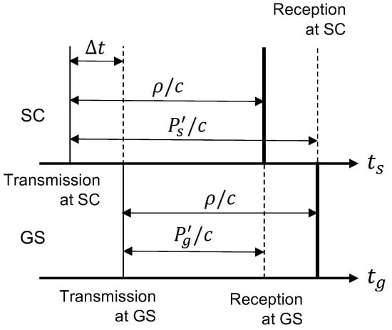
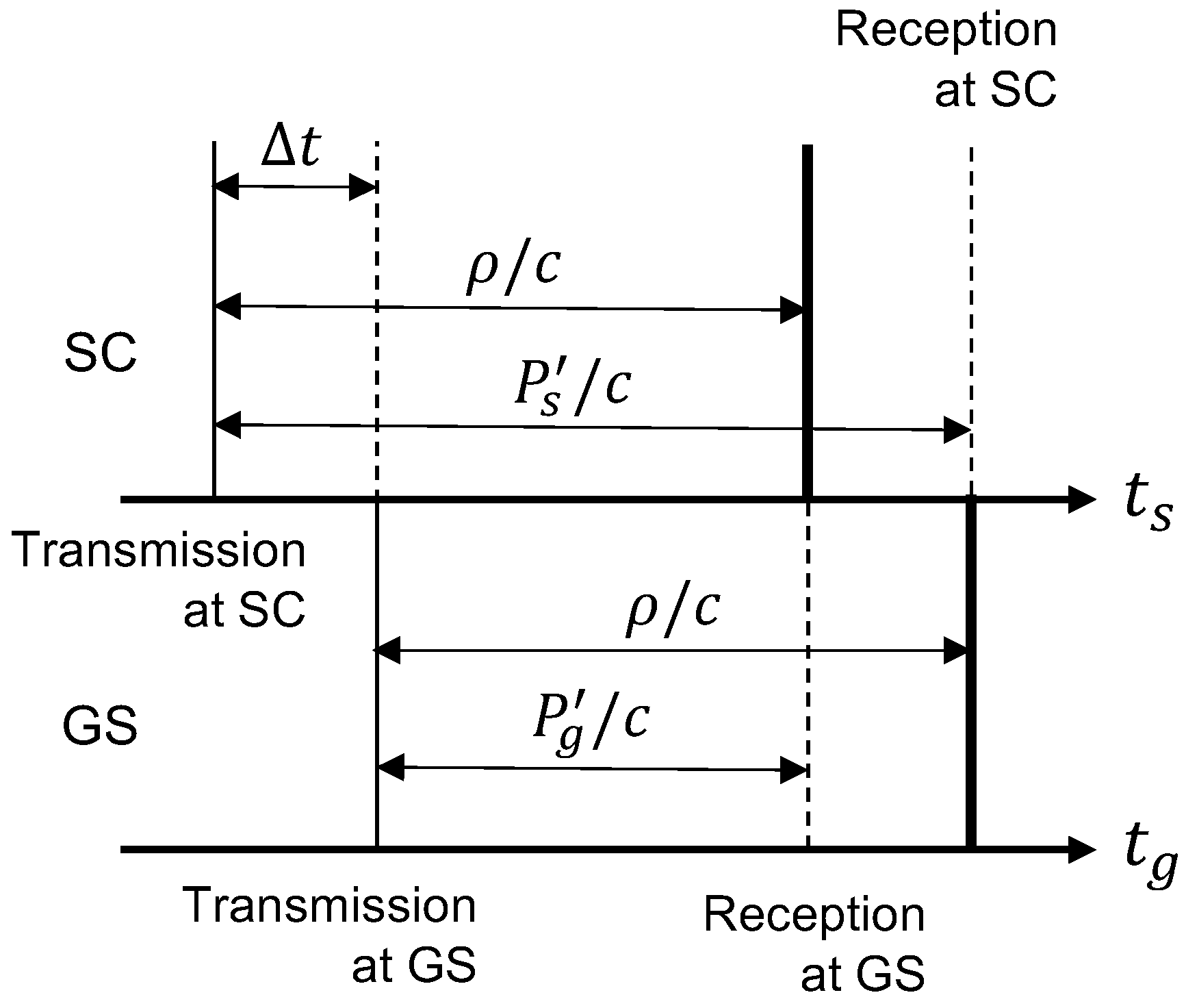
The fundamental principle of the AOWR method is briefly summarized here. Figure 1 illustrates the simplified signal flow between ground station (GS) and SC in the AOWR method.

Figure 1. Simplified signal flow in AOWR method (adapted from [19]).

Here, c is the speed of light; $t_g$ and $t_s$ denote the time systems of the GS and the SC, respectively; $\rho$ denotes the geometric range between the GS and the SC at the signal reception time; and $\Delta t$ represents the clock offset of the SC with respect to the GS. The quantities $P_g^{\prime }$ and $P_s^{\prime }$ denote the generalized pseudo-ranges (defined later in this section) for the GS and the SC, respectively.

The pseudo-range measurements obtained at the GS ($P_g$) and the SC ($P_s$) can be expressed, in their simplest form, as

$$\begin{array}{cc}\hfill P_g& =c(t_{gf}-t_{s0})=\rho -\Delta {\rho }_s-c\Delta t\hfill \end{array}$$

(1)

$$\begin{array}{cc}\hfill P_s& =c(t_{sf}-t_{g0})=\rho +\Delta {\rho }_g+c\Delta t\hfill \end{array}$$

(2)

where the subscripts 0 and f indicate the transmission and reception events, and $\Delta {\rho }_g$ and $\Delta {\rho }_s$ represent the position changes along the line-of-sight from the GS to the SC during the signal propagation period for the GS and the SC, respectively. Note that $t_g$ and $t_s$ are independent and asynchronous time systems; therefore, the reception times measured by the two clocks are not identical ($t_{gf}\ne t_{sf}$), even though the signal is received at the same physical instant. The clock offset is defined as $\Delta t=t_{sf}-t_{gf}$. Atmospheric effects are not considered here, as the intended application is small-body exploration.

Introducing the generalized pseudo-ranges of the GS ($P_g^{\prime }$) and the SC ($P_s^{\prime }$) yields the following relations:

$$\begin{array}{cc}\hfill P_g^{\prime }& \triangleq P_g+\Delta {\rho }_s=\rho -c\Delta t\hfill \end{array}$$

(3)

$$\begin{array}{cc}\hfill P_s^{\prime }& \triangleq P_s-\Delta {\rho }_g=\rho +c\Delta t\hfill \end{array}$$

(4)

When the GS is located on the Earth’s surface, $\Delta {\rho }_g$ can be computed using the ephemeris data and the Earth rotation model. If the GS is located on another celestial body, the corresponding ephemeris must be used. The term $\Delta {\rho }_s$ can be estimated by combining the line of sight (LOS) velocity derived from Doppler frequency measurements with the computed value of $\Delta {\rho }_g$. From the above relations, the summation and subtraction of the two measurements provide estimates of the geometric range and the clock offset, respectively:

$$\begin{array}{cc}\hfill \rho & ={\displaystyle \frac{1}{2}}(P_g^{\prime }+P_s^{\prime })\hfill \end{array}$$

(5)

$$\begin{array}{cc}\hfill \Delta t& ={\displaystyle \frac{1}{2c}}(P_s^{\prime }-P_g^{\prime })\hfill \end{array}$$

(6)

This formulation implicitly assumes that the pseudo-range measurements at the GS and the SC are obtained at the same physical instant. In practice, however, a time offset exists between the two measurements, and the resulting change in $\rho$ introduces an error in the AOWR observables. When the relative velocity between the GS and the SC is high, this reception-time mismatch becomes a non-negligible error source in the AOWR scheme. The resulting error in the estimated clock offset is approximately proportional to the reception-time offset multiplied by $\dot{\rho }/c+\dot{\Delta t}$, where $\dot{\rho }$ and $\dot{\Delta t}$ denote the range rate and clock drift rate, respectively. Because $\dot{\rho }/c+\dot{\Delta t}\ll 1$, even for a low-grade oscillator, the clock offset estimated by AOWR rapidly converges to the true value through iterative clock updates at the SC. Therefore, the errors in both clock offset and range estimation caused by the reception-time mismatch are negligible in practical operation.

Furthermore, carrier phase-based accurate ranging and clock synchronization have been proposed [21]. Similar to pseudo-range measurements, the generalized carrier phase measurements in the time domain, $C_g^{\prime }$ at the GS and $C_s^{\prime }$ at the SC, can be expressed in their simplest form as:

$$\begin{array}{cc}\hfill C_g^{\prime }& \triangleq C_g+{\displaystyle \frac{\Delta {\rho }_s}{c}}={\displaystyle \frac{\rho }{c}}-\Delta t-N_g{T}_g\hfill \end{array}$$

(7)

$$\begin{array}{cc}\hfill C_s^{\prime }& \triangleq C_s-{\displaystyle \frac{\Delta {\rho }_g}{c}}={\displaystyle \frac{\rho }{c}}+\Delta t-N_s{T}_s\hfill \end{array}$$

(8)

where $C_g$ and $C_s$ are the carrier phase measurements at the GS and SC, respectively; $N_g$ and $N_s$ are the phase ambiguities; and $T_g$ and $T_s$ denote the carrier periods of the downlink and uplink, respectively. Accurate range estimates based on the carrier phase measurements can then be obtained as

$$\begin{array}{c}\hfill \rho ={\rho }_{initial}+{\displaystyle \frac{c}{2}}(C_g^{\prime }+C_s^{\prime })\end{array}$$

(9)

where ${\rho }_{initial}$ represents the initial carrier phase offset and is estimated as follows. Note that ${\rho }_{initial}$ is distinct from the phase ambiguities $N_g$ and $N_s$:

$$\begin{array}{c}\hfill {\rho }_{initial}={\displaystyle \frac{1}{2n}}\sum _{i=1}^n\left\{{(P_g^{\prime }+P_s^{\prime })}_i-c{(C_g^{\prime }+C_s^{\prime })}_i\right\}\end{array}$$

(10)

Here, n denotes the number of subsequent measurements, and the subscript i indicates the measurement index. In the current implementation, the estimation of the initial carrier phase offset requires several minutes to converge, since a sufficient number of measurements must be accumulated to obtain a stable estimate. A detailed and rigorous derivation of this procedure is reported in [21]. The field experiment utilizes this carrier phase capability to achieve accurate positioning.

2.2. Implementation Aspect of AOWR

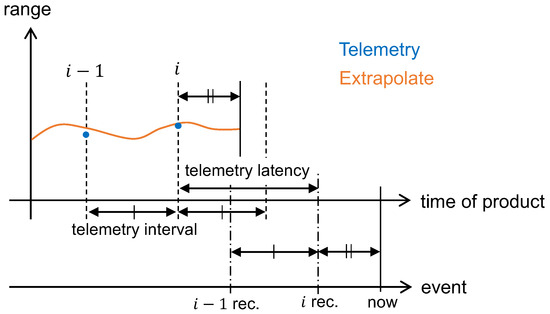
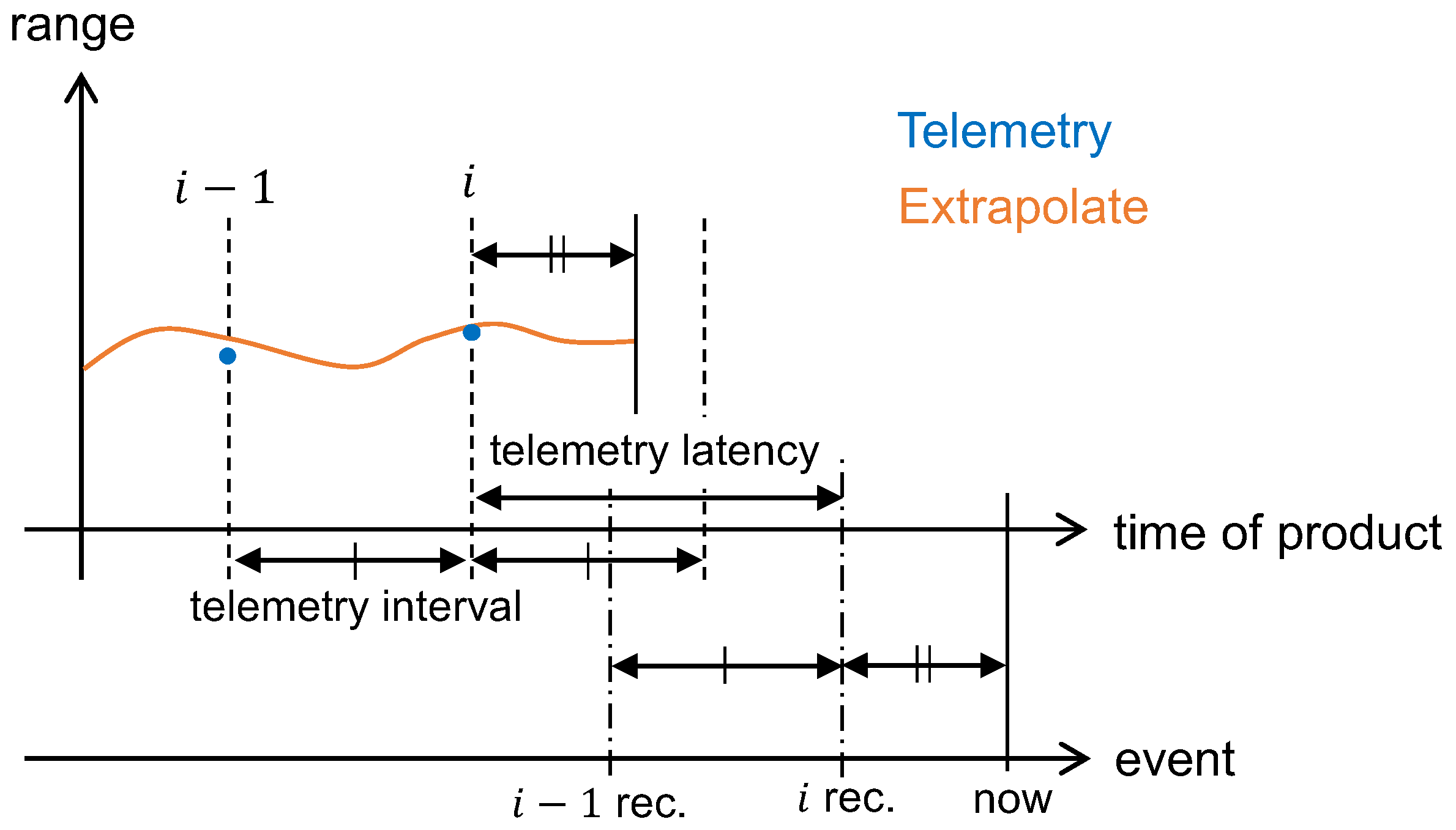
The authors developed the AOWR device and performed the field experiment [22]. The pseudorandom noise (PRN) code is used for timing measurements, and telemetry data are encoded on the code. Exchanging measured information introduces latency in the ranging and clock synchronization processes, due to both the finite length of the telemetry data and the signal propagation delay between distant entities. Figure 2 illustrates the relationship between the telemetry reception timing and the time tag of the telemetry. The blue dots represent the exchanged telemetry-based range observations. The notation i rec. indicates the reception timing of telemetry i, while its time tag corresponds to a past epoch, as indicated by i. Therefore, the difference between the reception timing and the time tag corresponds to the telemetry latency, as shown in Figure 2. The current implementation follows the heritage of the GPS L1 C/A architecture; therefore, the telemetry period is limited to every six seconds, corresponding to the subframe period of GPS L1 C/A. As a result, an approximately ten-second latency exists in obtaining the range and clock offset observations. Note that this telemetry frequency is not a fundamental limitation of the method and can be increased with a higher data rate, thereby reducing the latency.

Figure 2. AOWR observation latency and frequency. The upper and lower horizontal axes represent the time of product and the event timeline, respectively.

The pseudo-range and carrier phase measurements are continuously obtained while the tracking loop remains locked to the received signal, at intervals of 20 ms. For real-time positioning, both low latency and high-frequency range updates are essential. By using continuous tracking results, the clock offset can be extrapolated without requiring the counterpart’s measured information at the same epoch, thereby enabling continuous range estimation. Although the accuracy is degraded, the increased data frequency improves the usability of the positioning system for real-time autonomous operations. The current implementation estimates the clock drift rate from successive telemetry-based clock offset measurements and uses it to extrapolate the clock offset. Let $\Delta t_i$ denote the measured clock offset at epoch $t_i$. The clock drift rate ${\dot{\Delta t}}_i$ is computed using a backward difference approximation:

$${\dot{\Delta t}}_i={\displaystyle \frac{\Delta t_i-\Delta t_{i-1}}{t_i-t_{i-1}}}$$

(11)

The clock offset at time t is then extrapolated as

$$\begin{array}{c}\hfill \widehat{\Delta t}\left(t\right)=\Delta t_i+{\dot{\Delta t}}_i(t-t_i)\end{array}$$

(12)

To mitigate the impact of measurement noise, the clock drift rate can alternatively be estimated using a least-squares fit over multiple consecutive measurements. A more detailed derivation of this approach can be found in [23].

Figure 2 also illustrates the latency and update frequency of the extrapolated AOWR product. The arrows indicate the duration of the telemetry interval and latency. The notation “i rec.” denotes the reception of telemetry of epoch i, at which point the corresponding AOWR product becomes available. After the latest telemetry is received, the extrapolated product becomes available up to a time that is offset from the current time by the same latency as the telemetry-based product. Consequently, the extrapolated product has the same latency as the telemetry-based product, but provides data at a higher frequency of 20 ms.

3. Navigation System and Feasibility Study

3.1. AOWR Network-Based Positioning

The radio marker (RM)-based positioning system for the small-body sample-return mission is shown in Figure 3. The shown configuration uses only three RMs on the surface, which is the minimum configuration. More RMs can enhance the system robustness if the OTV and lander have a capability. When three or more ranges are obtained at the SC, the SC can determine its position autonomously. Here, the clocks of RMs are synchronized with the SC’s clock via the AOWR process without requiring the external time synchronization scheme, which is distinct from the UWB positioning. Therefore, the system can support the positioning of the lander in the landing phase and the relative positioning of the lander with respect to the OTV in the RVD phase.

Figure 3. Concept of positioning system for a small-body sample-return mission. Numbers indicate the IDs of the RMs.

The dilution of precision (DOP) is helpful to evaluate the expected positioning performance. Due to the limited size of small bodies, the baseline of RMs can be small compared to the distance of the SC to the surface. As a feature of the AOWR-based positioning, under such geometric circumstances, the vertical DOP (VDOP) can be negligible, which is different from the GNSS-based positioning. It is because there is no coupling between the vertical position component and the clock offset, since the AOWR observation provides the range but not the pseudo-range, which includes the clock offset. The lateral uncertainty or horizontal DOP (HDOP) is the same as when estimating the clock offset as well. Therefore, HDOP can be relatively large in this geometric condition.

Although the positioning accuracy degrades at larger distances from the surface, high accuracy is not required during the initial phase of the landing sequence. In this phase, the primary objective is coarse navigation to guide the lander toward the vicinity of the landing site. As the lander descends and approaches the surface, the measurement geometry improves, leading to a reduction in DOP and a corresponding increase in positioning accuracy. This characteristic is advantageous, as high positioning accuracy is most critical during the final approach and landing phase.

In contrast, during the RVD phase, the lander moves away from the RMs while the OTV remains at a relatively distant parking point. As a result, the relative position accuracy obtained by differencing the two independent positioning solutions may degrade due to unfavorable geometry. However, once the position of the OTV is determined in the local coordinate frame, it can be incorporated as an additional RM. This effectively improves the measurement geometry and reduces the DOP, thereby enabling practical relative positioning accuracy even in this configuration.

The preparatory operations required to construct the AOWR network-based self-positioning system around a small body are illustrated in Figure 4. First, the RMs are deployed by the lander prior to the landing phase. This preparatory approach can be performed multiple times to assess the terrain conditions and ensure a safe landing. The RMs can be released from an altitude of a few tens of meters above the surface, as demonstrated for TM deployment in the Hayabusa2 mission [3]. Placing the RM in the desired place precisely is technically challenging and not necessary. The marker location will be determined offline using a number of images. The lander can downlink images to the GS either directly or via the OTV when its communication capability is insufficient for direct communication with the GS. Determining the local coordinate system is performed using the location of RMs and terrain image data, and the location of RMs (${\mathbf{r}}_{\mathbf{1}},{\mathbf{r}}_{\mathbf{2}}$, and ${\mathbf{r}}_{\mathbf{3}}$) is defined in the local coordinate system. Since the accuracy of the location is limited by the accuracy of the image-based tracking data, the uncertainty information is also assumed to be generated. That information will be uploaded through the OTV to the lander.

Figure 4. Preparatory operation to construct AOWR network.

3.2. Radio Marker System

The RM deployed on the small body’s surface faces several system-level challenges, including power, thermal, and communication constraints. Furthermore, a lightweight and compact design is desirable due to the strict mass limitations of the overall spacecraft system. This study assumes a 1U (10 cm cube) form factor for the RM in the system design.

Because the power resources of the RMs are limited, the feasibility of establishing a reliable communication link must be verified. Table 1 summarizes the link budget calculation for the AOWR link at a distance of 50 km. Although the frequency selection is preliminary, the S-band is adopted in this analysis. For hemispherical coverage, the antenna boresight gain is assumed to be 3 dBi. A pointing loss is included when the link elevation deviates from the boresight direction. The transmission power is set to 1 dBm, which can be achieved using a software-defined radio (SDR) board without an additional power amplifier. The results indicate a sufficient link margin, demonstrating the feasibility of the communication link.

Table 1. AOWR link budget for radio marker and spacecraft.

Property	Unit	Uplink (RM to SC)	Downlink (SC to RM)
Frequency	MHz	2050	2285
TX Antenna		Patch	Patch
TX Ant Gain	dBi	3	3
TX Power	dBW	−30	−30
Feeder Loss	dB	2	5
TX EIRP	dBW	−29	−32
Free Space Path Loss	dB	133	134
(Distance)	km	50	50
Other Loss	dB	5	5
RX Ant Gain	dBi	3	3
Pointing Loss	dB	3	3
System Noise Temperature	dBK	26	26
RX C/No	dBHz	41	37
Modulation		BPSK	BPSK
Eb/No w/margin	dB	9.6	9.6
(BER)/code-pulse		${10}^{-5}$	${10}^{-5}$
(Property)		(20 ms, 0.5 MHz)	(20 ms, 0.5 MHz)
Bit Rate	dBHz	17	17
Required C/No	dBHz	27	27
Link Margin	dB	14	10

The feasibility from other system perspectives depends on the specific mission scenario; therefore, detailed analysis is beyond the scope of this paper.

3.3. Analysis of Expected Performance

This section presents a numerical analysis of the DOP for a landing probe on a small body. The simulation starts at an altitude of 1 km and ends at 10 m. The assumed trajectory is a constant-speed descent toward the landing site, taking into account the rotation of the small body about its body-fixed z-axis. This trajectory is illustrated by the blue line on the right-hand side of Figure 5 and is expressed in the body-fixed frame. The red points represent the locations of the RMs, the green dashed lines indicate the LOS directions from the RMs to the SC at the beginning of the simulation, and the gray sphere is the surface of the small body. The rotation period of the small body is assumed to be 15 h, the radius is 500 m, and the shape is modeled as a sphere. The descent phase lasts for 1 h. To account for terrain occultation of the radio link from the RMs to the SC, a minimum elevation angle of 5 deg is adopted as the visibility condition. Although the visibility condition depends strongly on the shape of the small body, more realistic geometric effects, such as deviations from a spherical shape (e.g., oblate or irregular forms), are beyond the scope of this study.

Figure 5. History of DOP and visible RMs and lander’s trajectory.

The left-hand side of Figure 5 shows the DOP history of the lander and the number of visible RMs when four RMs are used with a displacement angle of 20 deg from the body’s center-to-landing-site LOS direction. The displacement angle is defined as $arccos({\overrightarrow{r}}_{land}·{\overrightarrow{r}}_{RM})/\left(\right|{\overrightarrow{r}}_{land}|·|{\overrightarrow{r}}_{RM}\left|\right)$, where ${\overrightarrow{r}}_{land}$ and ${\overrightarrow{r}}_{RM}$ denote the position vectors of the landing site and the RM, respectively, measured from the center of the small body. The position DOP (PDOP) starts at approximately 8 and decreases as the SC approaches the surface. Note that PDOP and HDOP show similar values, while VDOP remains close to 1, which is a characteristic feature of AOWR-based positioning. At an altitude of approximately 60 m, the number of visible RMs becomes fewer than three due to terrain occultation; therefore, the DOP cannot be computed below this altitude. Under this configuration, the PDOP decreases to approximately 1.5 near the end of the descent, indicating that sufficient positioning accuracy can be achieved for landing.

Figure 6 shows the maximum PDOP and the minimum altitude at which at least three radio links are available, as functions of the number of RMs and their displacement angles. In this analysis, the same SC trajectory as shown in Figure 5 is assumed. Although the placement of RMs is an important factor, one marker is placed at the landing site, while the others are placed at the maximum displacement angle and are evenly distributed in azimuth direction. When the distance between the RMs, i.e., the baseline of the network, increases, the HDOP decreases. However, at lower altitudes, the SC cannot maintain a sufficient number of ranging links with the RMs due to terrain occultation. Therefore, a trade-off relationship appears between the maximum PDOP and the minimum altitude at which positioning is available, as shown in Figure 6.

Figure 6. Maximum PDOP and minimum altitude for positioning by RMs depending on the number of markers and displacement angles.

In the present descent scenario, the maximum PDOP occurs at the initial phase of the descent; therefore, the positioning accuracy improves as the SC approaches the surface. Note that the DOP values strongly depend on the geometric placement of the RMs, and the present analysis corresponds to one representative configuration. An optimization study of beacon placement for a similar positioning system applied to Mars landing is reported in [24]. As shown in Figure 6, increasing the number of RMs and the displacement angle improves the PDOP, because the baseline of the network becomes larger and the HDOP, which dominates the PDOP, decreases. In addition to the DOP, the positioning accuracy is also discussed in the following section based on the actual ranging results obtained from the field experiment.

Regarding the minimum altitude for positioning, the current analysis is limited to an altitude of 10 m; therefore, positioning is available throughout the descent when the displacement angle is 5 deg. As the displacement angle increases, the minimum altitude for positioning also increases because the RMs are more likely to be hidden by the terrain of the small body. The number of RMs does not significantly improve the minimum altitude for positioning; rather, it strongly depends on the displacement angle. This is because the current marker placement focuses on the maximum displacement angle, and the elevation angles of the RMs with respect to the SC become low, since most markers are located far from the landing site. It should be noted that the final approach phase is expected to be supported by alternative navigation methods, such as vision-based navigation; therefore, maintaining radio-based positioning down to a few tens of meters is sufficient for the proposed system.

4. Field Experiment

4.1. Experiment Overview

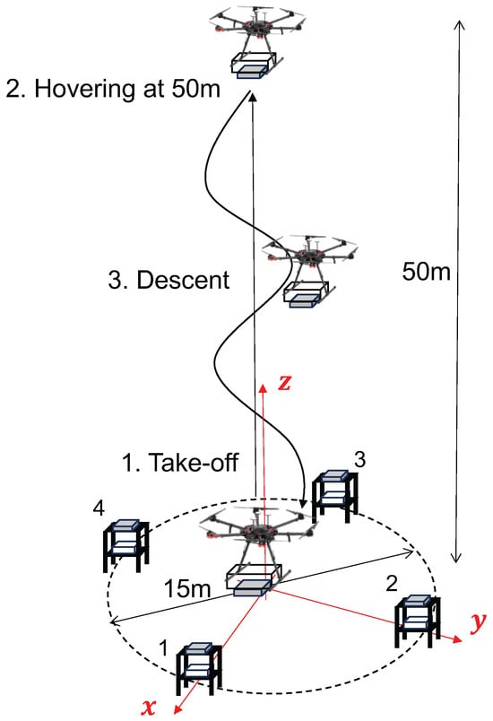
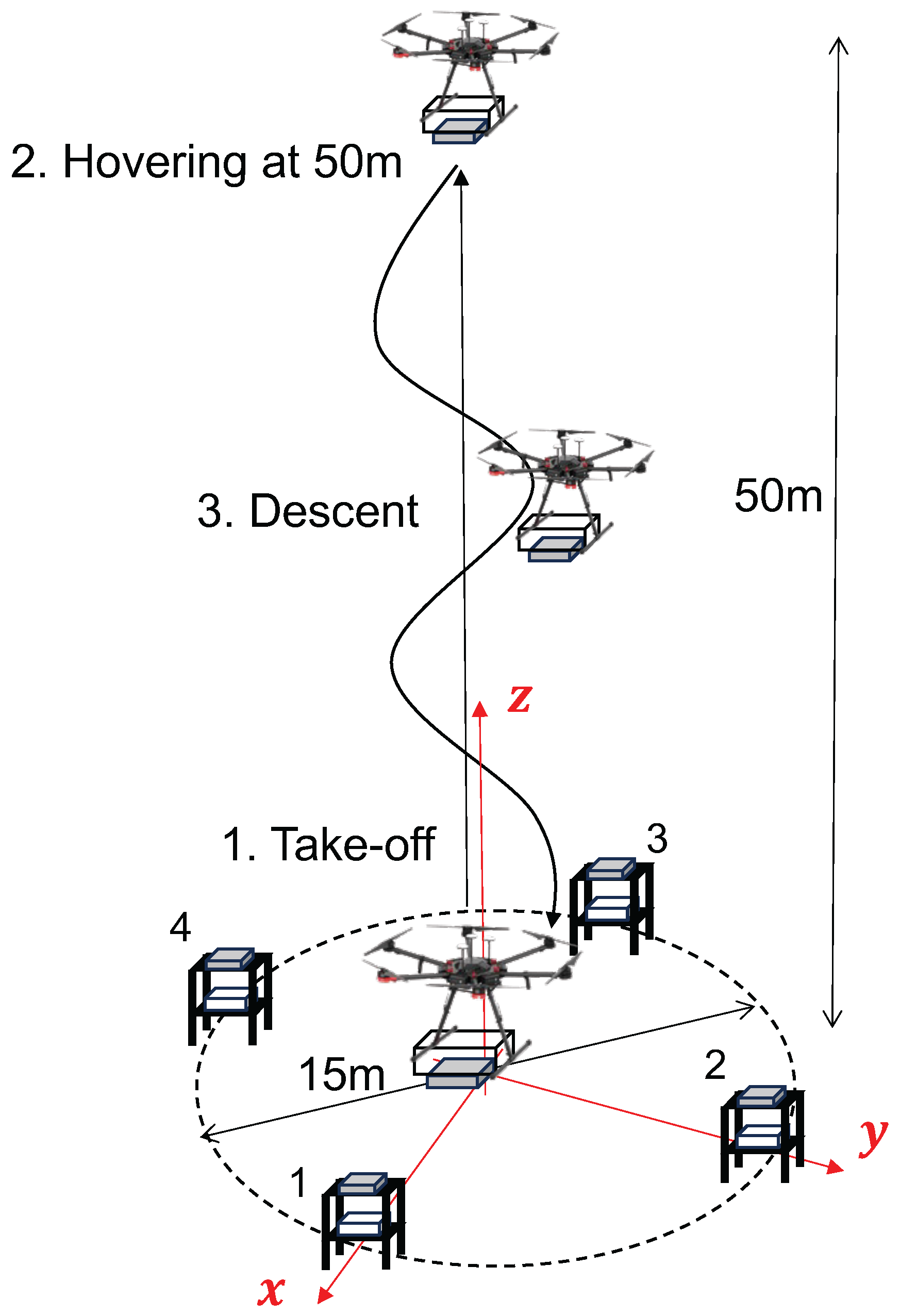
The positioning capability of the AOWR network was demonstrated using a drone and RMs. The configuration is shown in Figure 7.

Figure 7. Drone field experiment configuration and procedure.

Four markers are placed on a circle with a diameter of 15 m. Although, in theory, the position can be determined using at least three range measurements obtained from the AOWR, an additional marker is introduced to improve robustness against link disconnection and to enhance positioning accuracy. The local coordinate system is defined as shown in Figure 7, where the origin is located at the center of the circle. The x-axis is aligned with the line connecting marker 1 and marker 3, the y-axis is orthogonal to the x-axis and aligned with the line connecting marker 2 and marker 4, and the z-axis completes the right-handed coordinate system. The antenna locations of the markers are defined in meters as follows: 1: $(7.5,0.0,0.7)$, 2: $(0.0,7.5,0.7)$, 3: $(-7.5,0.0,0.7)$, 4: $(0.0,-7.5,0.7)$. In the actual experiment preparation, the marker’s location is precisely measured by the tape measure and placed on the designated places.

The experiment procedure is defined to start with hovering at the maximum height (50 m) and then descending toward the surface in order to avoid multipath reflections from the ground at the initial phase. In addition, the initial carrier phase offset estimation described in Section 2 is required to refine the ranging accuracy, and this process takes a few minutes in the current implementation. Considering the intended application to small-body exploration, the distance between the small-body surface and the SC is initially large and gradually decreases as the spacecraft approaches the surface. Accordingly, the experimental procedure is designed to emulate the landing phase of the mission scenario. Positioning is performed via least-squares estimation based on the range measurements. For evaluation of the positioning performance, the GNSS-based position provided by the drone is used as a reference for comparison.

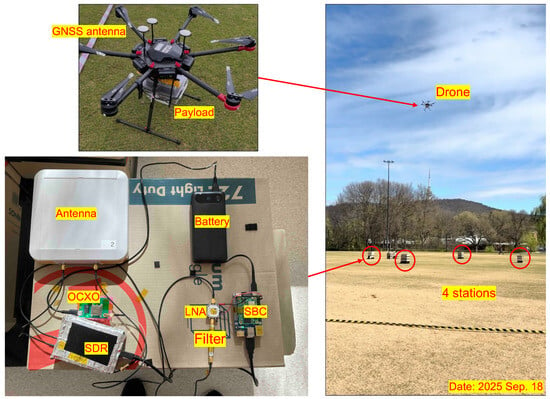
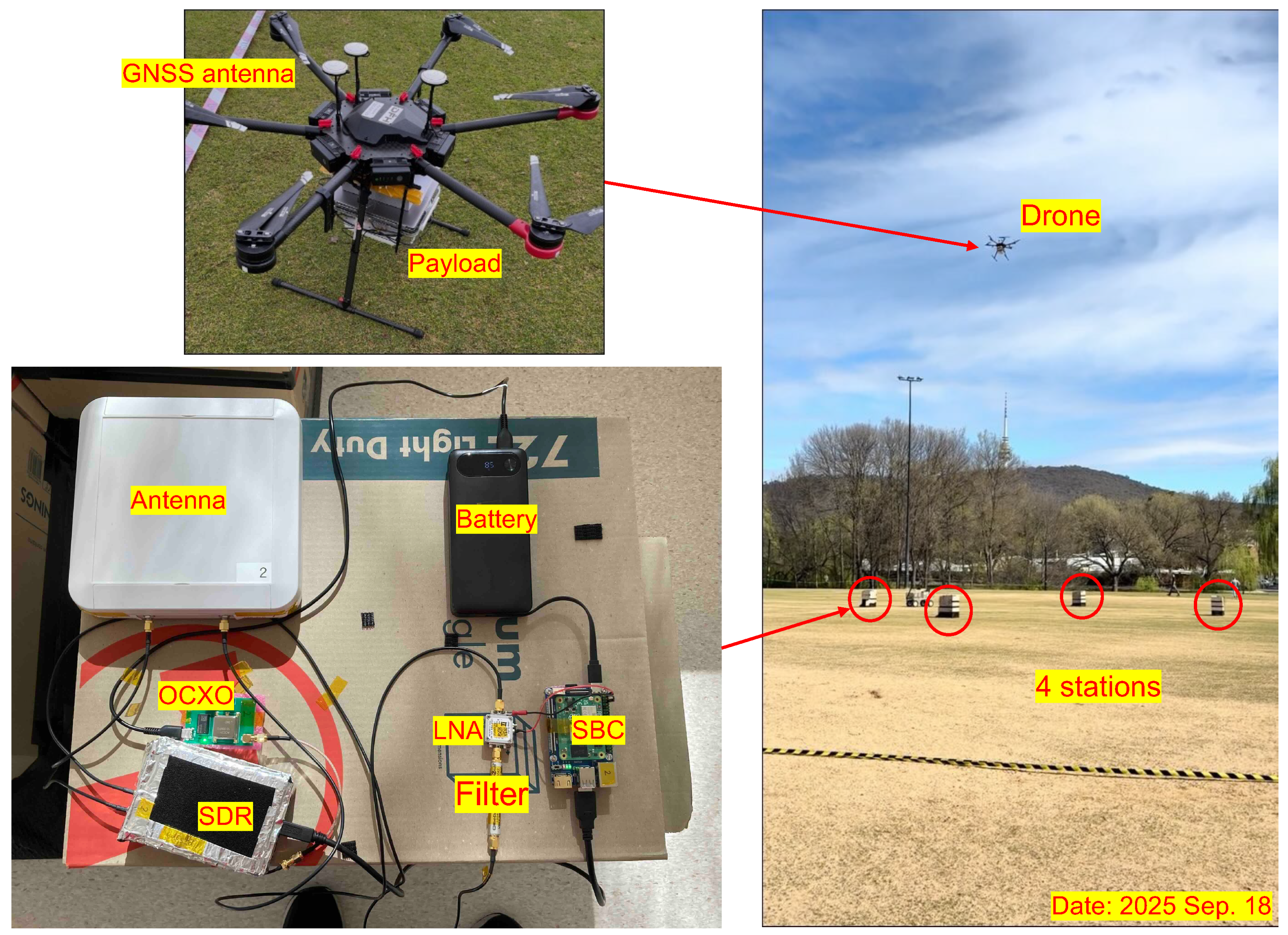
The experiment components and the actual configuration of the field demonstration are shown in Figure 8. The drone used in the experiment is a DJI Matrice 600 Pro, and the payload for AOWR ranging is mounted on the drone. The built-in GNSS antenna and receiver are used only for post-experiment comparison with the estimated position data. Platform-type markers (bottom left in Figure 8) are used in this experiment. Cardboard is selected as the platform material to minimize radio signal reflections from the marker structure. The onboard battery supplies power to the single board computer (SBC), SDR transceiver, oven-controlled crystal oscillator (OCXO), and low noise amplifier (LNA). The SBC processes the data sampled by the SDR. The same type of antenna is employed on the drone, featuring a relatively narrow radiation pattern with a half-power beamwidth of approximately 20°. To establish four ranging links simultaneously, independent PRN codes are assigned to each marker. The Wi-Fi band was selected for the operating frequency. The right-hand side of Figure 8 shows the actual flight scene during the experiment.

Figure 8. Experiment components and field demonstration.

4.2. Experiment Results

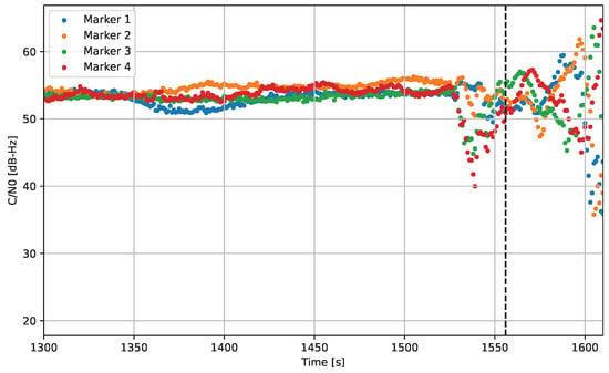
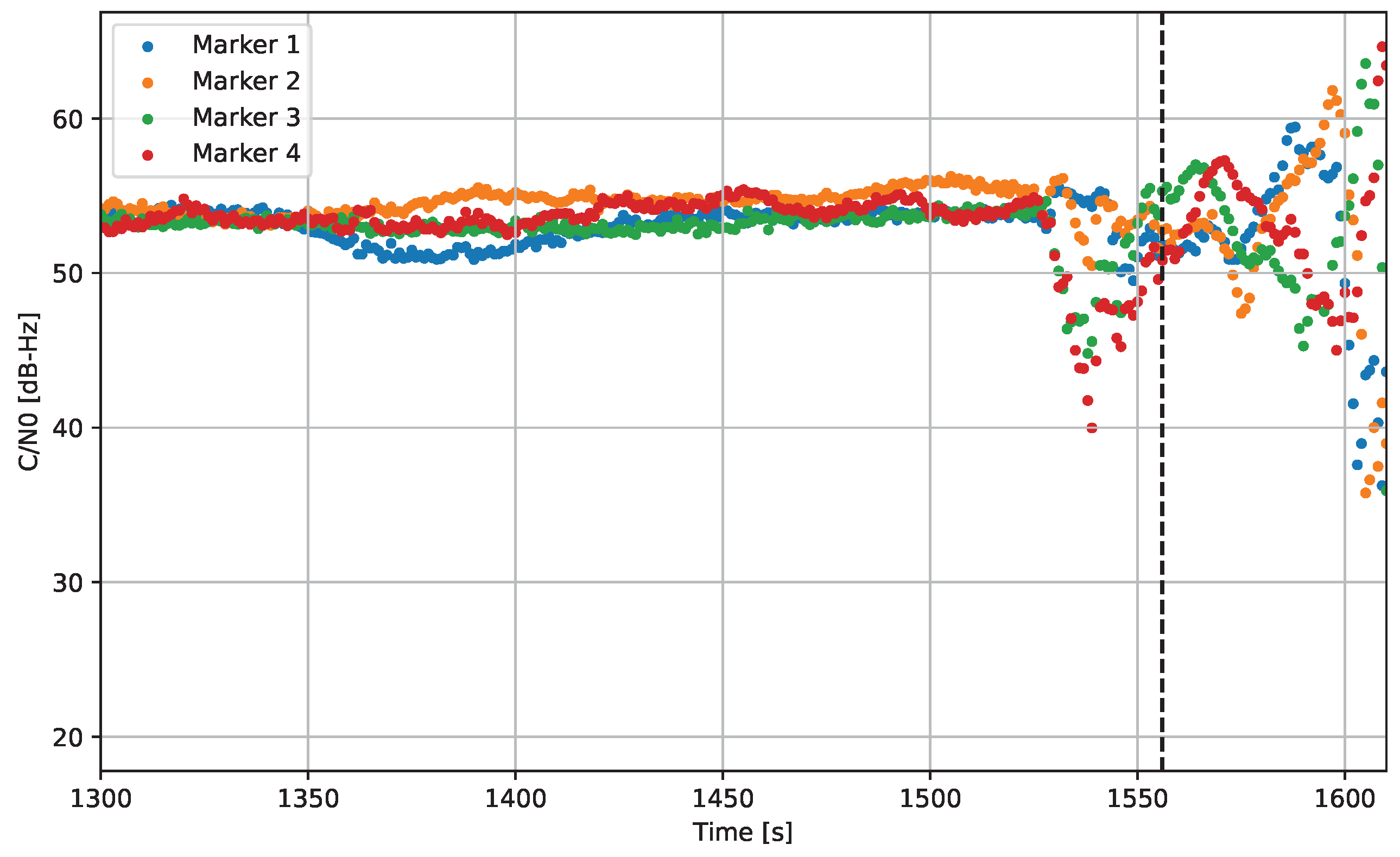
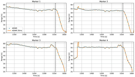
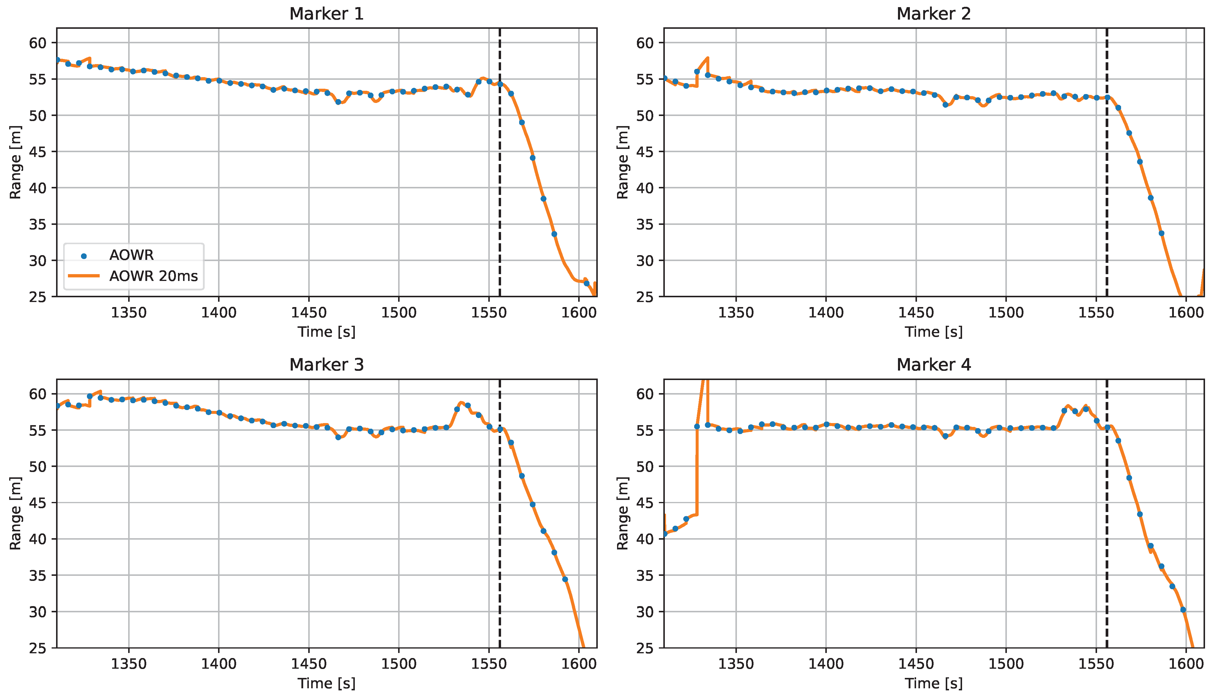
Figure 9 and Figure 10 show the history of carrier-to-noise density ratio (C/N0) and the range measurements obtained by the drone. The horizontal axis represents the AOWR local time in seconds. The C/N0 data, only when the ranging link is established, is shown. In Figure 10, “AOWR” denotes the telemetry-based range, while “AOWR 20 ms” represents the extrapolated range obtained at 20 ms intervals.

Figure 9. C/N0 history of drone. The vertical dashed line indicates the start of the descent.

Figure 10. Range history measured by drone. The vertical dashed line indicates the start of the descent.

During hovering, the C/N0 remains stable at more than 50 dB-Hz, and the measured ranges remain nearly constant until approximately 1520 s. After this point, the drone begins to move, and a circular descent phase starts, as indicated by the dashed line in Figure 9. During the motion phase, the C/N0 fluctuates due to attitude variations of the drone, which alter the elevation angle of the links and thus the effective antenna gain, while remaining above 40 dB-Hz. Furthermore, from the descent phase onward, the range values begin to decrease, as shown in Figure 10. After 1600 s, the ranging links are disconnected, and the range measurements become unavailable as the altitude of the drone decreases. Because the antenna pattern used in this experiment is relatively narrow, sufficient link margin cannot be maintained when the elevation angle becomes low. In contrast, the antenna assumed for the small-body exploration scenario provides hemispherical coverage; therefore, continuous ranging is expected to be maintained over a longer duration.

Regarding the extrapolated range, the results show good agreement with the telemetry-based range, as illustrated in Figure 10. At the initial phase, small jumps can be observed between successive telemetry updates, since the estimated clock offset is not yet sufficiently accurate due to the limited accuracy of the telemetry-based solutions, which is caused by the incomplete convergence of the initial carrier phase offset estimate (see the following paragraph for details). However, this estimation improves over time, and the extrapolated range smoothly connects the telemetry-based solutions.

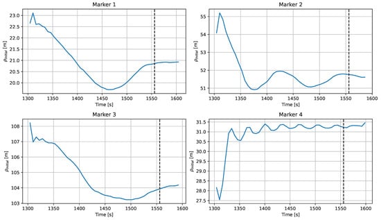
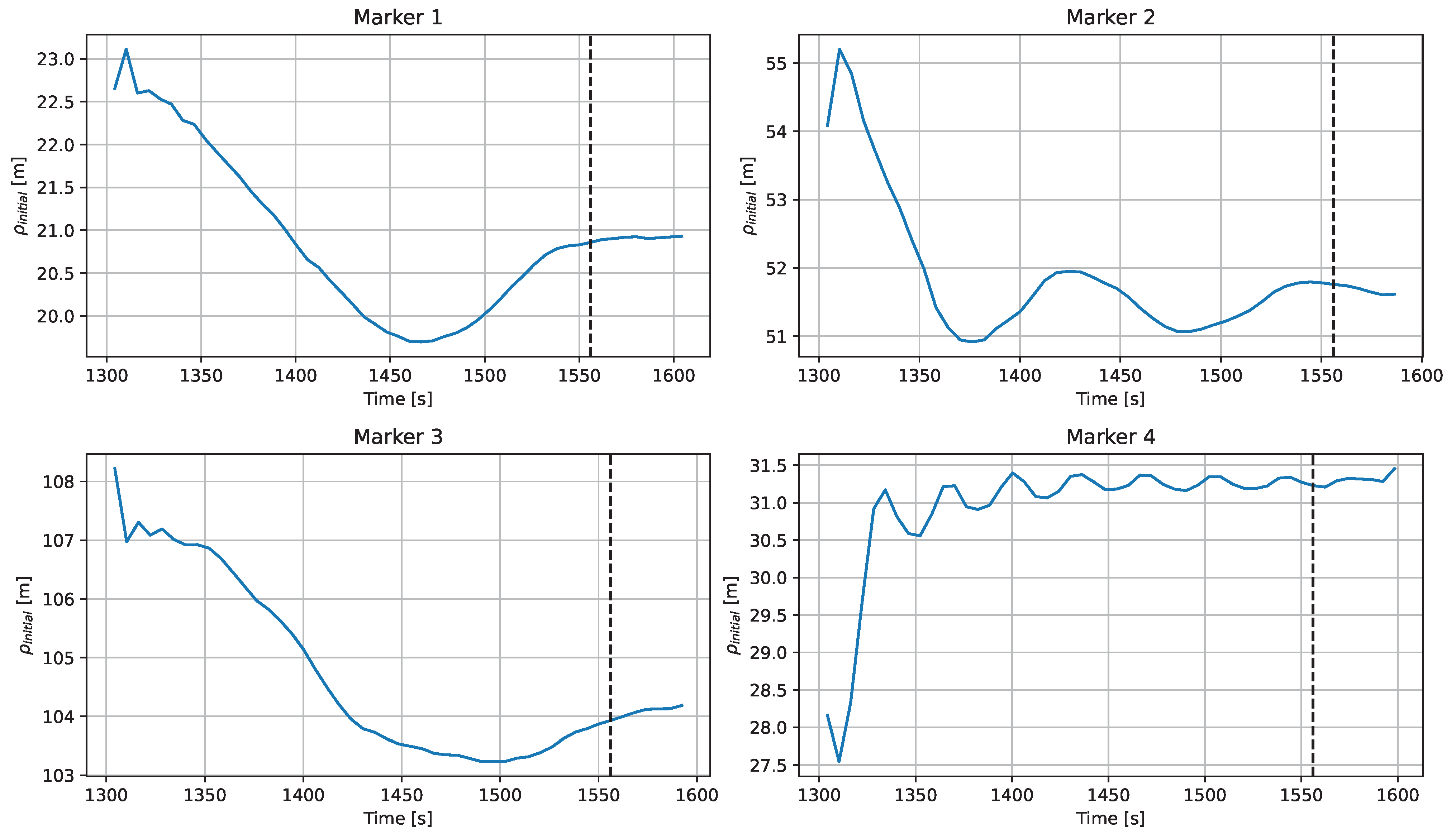
The initial carrier phase offset estimation results are shown in Figure 11 in units of meters for each RM. The estimated values and their convergence behavior differ among the RMs. The authors observed a sinusoidal variation in the estimated profiles, and the period of this variation depends on the clock drift rate of each RM relative to the drone clock. Specifically, markers 1 and 3, whose clock drift rates are small, exhibit very long periods, whereas marker 4, whose clock drift rate is large, shows a faster variation. Although the amplitude of the variation is within approximately 5 m in all cases, marker 4 reaches a value close to the final solution in a relatively short time, while the markers with longer periods continue to exhibit drifting behavior throughout the ranging interval. This slow convergence results in a residual bias in the ranging measurements.

Figure 11. Initial carrier phase offset estimation process. The vertical dashed line indicates the start of the descent.

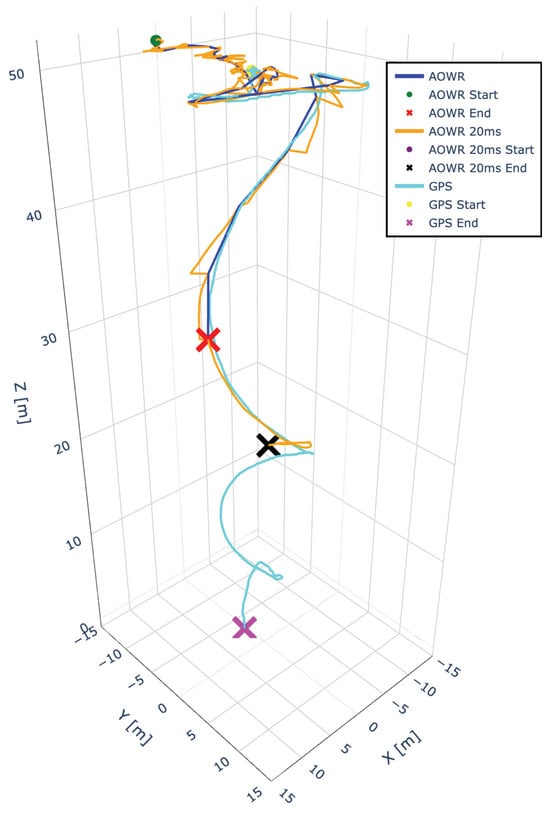
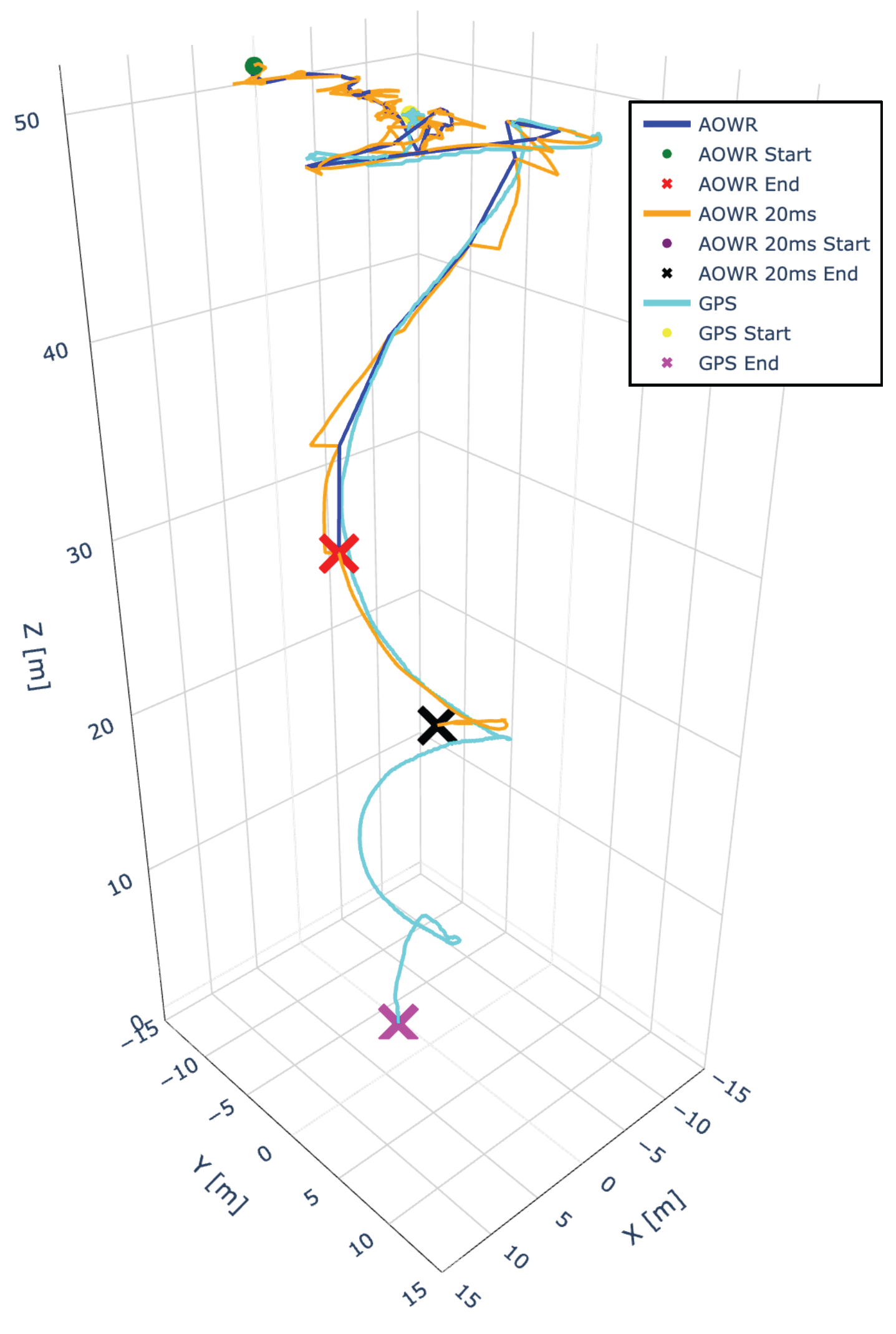
Figure 12 shows the positioned drone trajectory by different methods. The data label “AOWR” indicates the position obtained using the telemetry data, which is every six seconds, “AOWR 20ms” is for those obtained from the extrapolated range, and the “GPS” is for those obtained from the GNSS receiver. The position is expressed in the local coordinate system shown in Figure 7; thus, the GNSS-based position obtained in Earth-centered, Earth-fixed (ECEF) frame is converted.

Figure 12. Positioning results comparison in 3D plot.

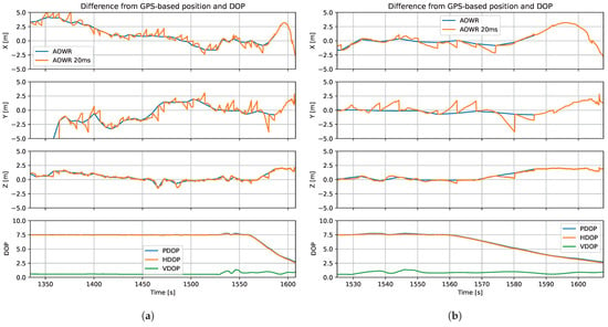
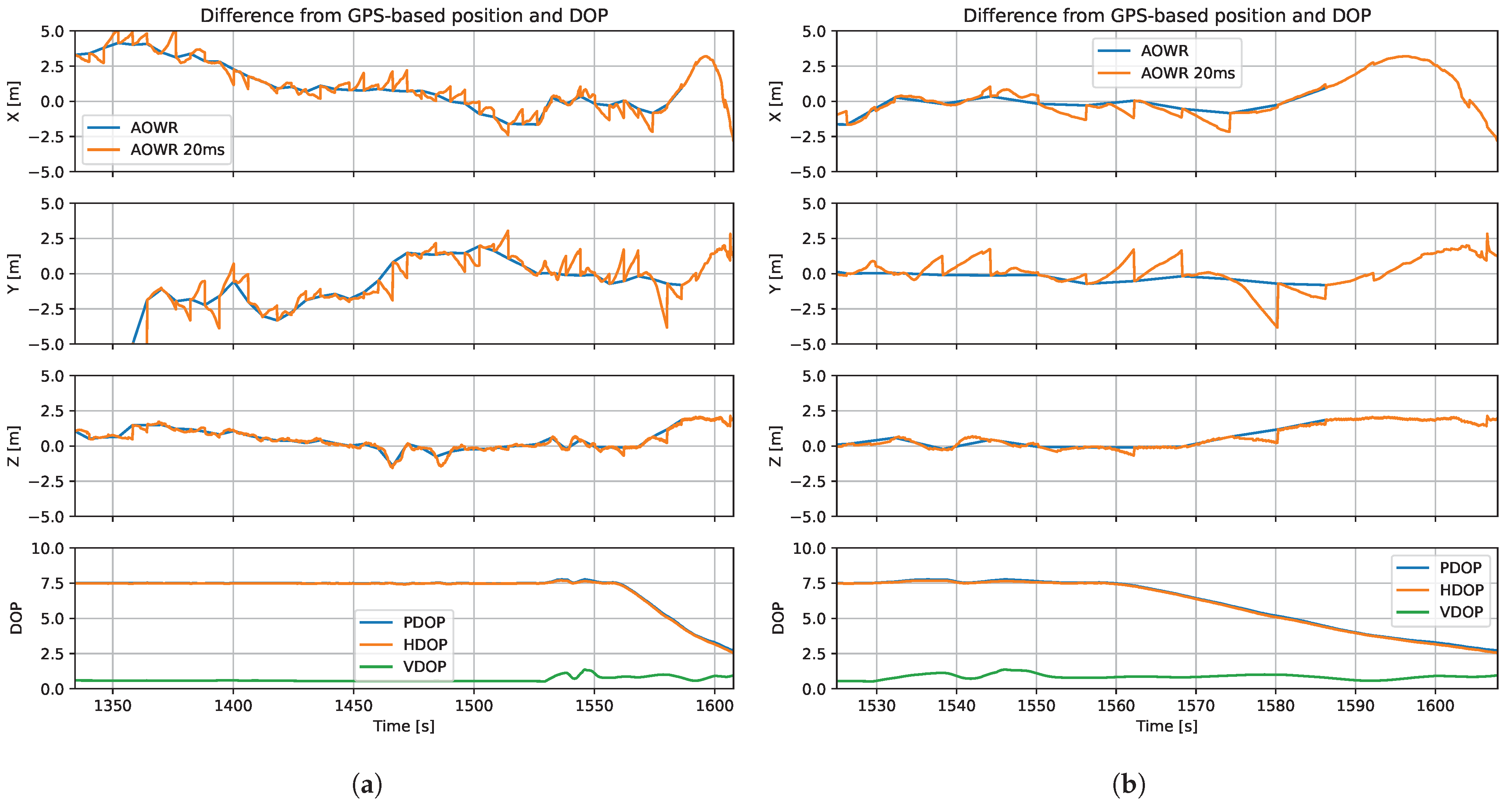
Figure 13a,b show the difference from the GNSS-based positioning result and DOP over the experiment duration, and its enlarged view during the motion phase, respectively. In both figures, the first three rows show the difference from the GNSS-based position in x, y, and z axes of the local coordinate, and the bottom row shows the DOP history of the AOWR-based positioning during the flight. Note that it is not the absolute positioning error but the difference from the GNSS-based positioning results, as no truth position is available. The horizontal axis indicates the local time of the AOWR system.

Figure 13. Position difference from GPS-based position and DOP over the entire experiment duration (a) and during the motion phase (enlarged view) (b).

Initially, the AOWR-based position differs from the GNSS-based position, especially in the y-direction. This is because the estimation of the initial carrier phase offset is not sufficiently accurate, as shown in Figure 11. The estimation converges after several hundred seconds, and the estimated position then matches the GNSS-based position. Although the experimental results show limited accuracy in the initial phase, the authors found that using an independent sampling rate at the ranging entities accelerates the estimation of the initial carrier phase offset even when the clock drift rate is low. Therefore, the initialization phase can be accelerated in future studies.

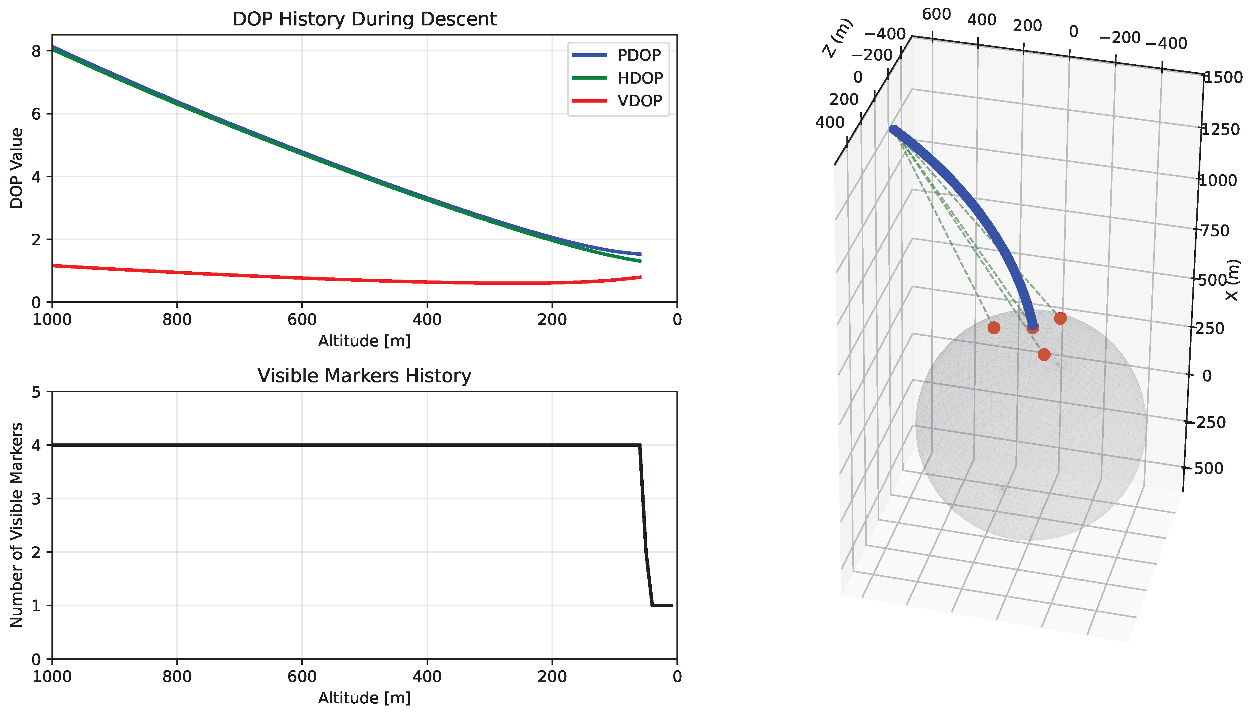
After the initial carrier phase offset is estimated with practical accuracy, the position difference from the GNSS-based position is within a few meters, while the DOP is approximately 7.5. This implies that the ranging accuracy is at the sub-decimeter level. As seen in the DOP plots in Figure 13b, the descent phase starts around 1560 s, and the profile during the descent is nearly identical to the numerical analysis shown in Figure 5. Therefore, similar positioning performance can be expected in the small-body landing scenario. Furthermore, the HDOP is much larger than the VDOP in this geometric configuration. Due to the relatively large HDOP, the errors in the x- and y-axes reach a few meters, while the error in the z-axis remains within one meter.

The extrapolated solution, “AOWR 20 ms”, slightly deviates from the exchanged-telemetry-based solution, “AOWR”. This difference is caused by extrapolation errors between telemetry intervals, which are corrected upon reception of new telemetry. The discrete steps observed in the position difference arise from this clock offset update at each telemetry epoch. Between updates, the clock offset is extrapolated, leading to a gradual accumulation of error, which is then corrected when new telemetry is received, resulting in a corresponding discontinuity in the position solution. This behavior is inherent to the discrete telemetry update scheme and does not indicate instability in the positioning algorithm.

Although the extrapolated range remains well aligned with the telemetry-based range, as shown in Figure 10, noticeable deviations appear in the position-domain results. This is because the position error is amplified by the DOP, which acts as a geometry-dependent scaling factor. Furthermore, the difference in the magnitude of the deviation between the horizontal and vertical components is attributed to the imbalance between HDOP and VDOP, where HDOP dominates in the current geometry.

In Figure 12, the position results of AOWR end earlier than the GNSS-based results because the ranging link is disconnected at low altitude, as described above. Additionally, the exchanged telemetry-based results, “AOWR”, end earlier than the extrapolated results, “AOWR 20 ms”. This is because the ranging solution based on exchanged telemetry relies on past measurements. Consequently, the telemetry-based solution remains available until the time corresponding to the last successfully exchanged telemetry, whereas the extrapolated results remain available up to the actual time of link disconnection. In the final phase, the position error of the extrapolated results increases even though the DOP values decrease. This occurs because the clock extrapolation accuracy degrades in the absence of correction from telemetry-based ranging results. Moreover, multipath effects from the ground surface become more significant at low altitude, further degrading the ranging accuracy.

Table 2 summarizes the root mean square (RMS) position differences of the proposed method with respect to the GNSS-based positioning results. The differences are evaluated over both the entire period and the motion phase only, corresponding to Figure 13b. Due to geometric constraints reflected in the DOP, the horizontal error is larger than the vertical one. Over the entire period, the 3D RMS difference is approximately 4 m, primarily due to the inaccurate estimation of the initial carrier phase offset. In contrast, during the motion phase, the accuracy improves to approximately 1 m for the telemetry-based results and 2 m for the extrapolated results. These results are single-point positioning results obtained without sequential filtering; therefore, further improvements in positioning accuracy are expected when incorporating a dynamic model and applying state-estimation-based filtering.

Table 2. Summary of position difference from GNSS-based solution in RMS.

	Entire Period			Motion Phase
Method	Horizontal (XY)	Vertical (Z)	3D	Horizontal (XY)	Vertical (Z)	3D
Telemetry-based	3.88	0.76	3.96	0.81	0.73	1.09
Extrapolated	3.75	0.86	3.85	1.68	1.07	1.99

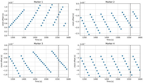
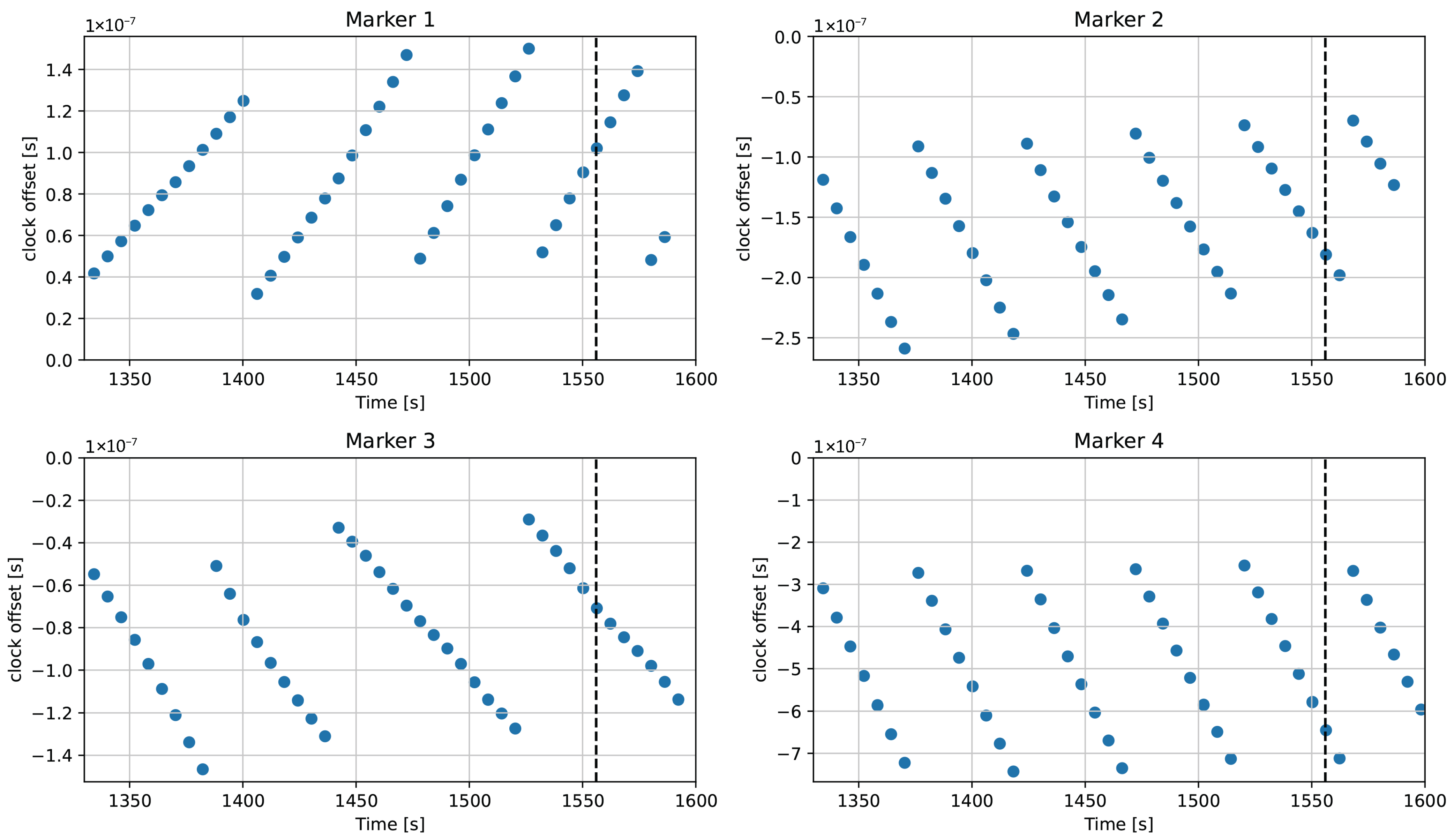
Figure 14 summarizes the estimated clock offsets of the four RMs with respect to the drone. Depending on the clock drift rate, the clock offset either increases or decreases over time. The data are shown at six-second intervals (telemetry period), so the change between successive points corresponds to the clock drift over six seconds. The periodic step-like behavior indicates that the clocks of the RMs are actively corrected to suppress the magnitude of the clock offset. This correction is essential, as a large clock offset leads to errors in both ranging and clock offset estimation due to the effects of range rate and clock drift, as described in Section 2. The results demonstrate that the AOWR method successfully estimates the clock offsets of multiple entities simultaneously, thereby achieving simultaneous clock synchronization. The observed clock drift rates, derived from the time history of the estimated clock offsets, are approximately as follows: marker 1: 2 ppb, marker 2: −3 ppb, marker 3: −1 ppb, and marker 4: −11 ppb. The relatively large drift rate of marker 4 is consistent with the faster convergence behavior of the initial carrier phase offset estimation shown in Figure 11.

Figure 14. Measured clock offsets of four RMs. The vertical dashed line indicates the start of the descent.

Regarding the extrapolation error in “AOWR 20ms” in Figure 13b, the solution deviates by a few meters from the exchanged-telemetry-based position until approximately 1570 s. During this period, the PDOP is approximately 7, and the telemetry interval is six seconds. Assuming a position error of approximately 3 m, the corresponding range error per link can be approximated as 3 m/7. Dividing this by the telemetry interval yields an equivalent range-rate error of (3/7)/6 m/s. Converting this to a clock drift rate error by normalizing with the speed of light gives an approximate drift rate error of 0.24 ppb. The estimation accuracy can be improved by using multiple observations to estimate the clock drift rate. Additionally, shortening the telemetry interval can mitigate the ranging error caused by clock drift estimation errors by enabling more frequent updates.

4.3. Applicability to Small-Body Mission

The differences between the drone-based experimental environment and the small-body exploration scenario are examined in this section.

The lateral offsets from the centroid of the RMs can occur during the initial phase of landing in practical small-body missions. Although the flight experiment was conducted with the drone initialized above the centroid of the RMs, the positioning framework is not limited to this configuration. Numerical results show that lateral offsets degrade the positioning geometry, primarily affecting the horizontal component. For example, at an altitude of 1 km, the configuration with lateral offset yields approximately PDOP ≈ 8, HDOP ≈ 8, and VDOP ≈ 1, as shown in Figure 5, whereas the zero-offset case results in lower values of approximately PDOP ≈ 7, HDOP ≈ 7, and VDOP ≈ 0.5. This indicates that the degradation is primarily driven by an increase in HDOP.

This behavior is attributed to the characteristics of the AOWR formulation, in which clock ambiguity is eliminated and the marker baseline is small relative to the radial distance. As a result, the positioning accuracy is dominated by the horizontal geometry. Although VDOP is also affected by lateral offsets, its contribution to the overall positioning error remains secondary. As discussed in Section 3, high positioning accuracy is not required at large distances from the surface, where the primary objective is coarse navigation toward the landing site. As the probe descends, the measurement geometry improves, leading to reduced DOP values and enhanced positioning accuracy during the final approach phase, where precise navigation is critical.

In addition, the scale differs significantly, with the experiment conducted at altitudes up to 50 m, whereas the mission scenario extends to approximately 1 km. However, since the positioning accuracy is primarily governed by the DOP and the ranging accuracy, and the DOP values are comparable across these scales, the impact of scale is limited, provided that sufficient ranging accuracy is maintained.

Differences in signal conditions may also affect ranging performance. While the experiment assumes strong signal conditions, the small-body scenario may experience reduced signal strength. Nevertheless, given the sufficient link margin shown in Table 1, the resulting positioning accuracy is expected to remain comparable.

Based on the computed DOP values, the expected positioning performance in the small-body scenario is consistent with the experimental results, with moderate degradation under non-ideal geometric conditions.

5. Conclusions

This study proposed a standalone self-positioning system for a small-body sample-return mission. The positioning system is based on multiple RMs deployed on the surface of the small body and is applicable to both surface landing and ARV in a multi-spacecraft mission architecture. The ranging method is AOWR, which enables simultaneous ranging and clock synchronization among multiple entities. This capability allows positioning without requiring external time-synchronization means, unlike UWB-based positioning, because the SC plays the role of a master clock and distributes time to all RMs. Additionally, this consolidated feature allows the mother SC, or OTV, to function as an additional RM for the ascending probe during the ARV phase.

This paper demonstrated the operational procedure of the RM-based positioning system for a small-body sample-return mission, the preliminary ranging link feasibility of the RM system under strict size and power constraints, and numerical analysis of the expected positioning performance for the landing scenario. Furthermore, a field experiment using a drone was conducted to validate the positioning capability of the proposed AOWR-based network approach. The experimental results demonstrate that the proposed system can achieve simultaneous clock synchronization and ranging among multiple entities, with positioning accuracy comparable to GNSS-based measurements in a ground experiment. This indicates that comparable positioning performance can be expected for small-body exploration applications. The positioning accuracy analysis, accounting for DOP, indicates that the ranging accuracy can be expected to reach the sub-decimeter level.

For future work, positioning simulations incorporating a realistic dynamical model around the small body are essential to evaluate system performance in actual mission conditions. The uncertainty in the RMs’ locations may affect positioning accuracy; however, once a suitable dynamics model is available, it should be possible to refine the RM locations using multiple ranging data with the spacecraft. This numerical verification is left for future studies. In addition, to utilize the OTV as an additional RM for ARV, broadcasting the OTV position is required. This would necessitate exchanging additional data, potentially increasing telemetry length and introducing slight latency in range measurements. Moreover, the positioning accuracy of the OTV directly influences the relative navigation accuracy of the lander. Investigating these aspects is therefore crucial for fully demonstrating the feasibility of the proposed system. Therefore, demonstrating the feasibility of the relative navigation using two drones is planned for future work.

References

- Ge, D.; Cui, P.; Zhu, S. Recent development of autonomous GNC technologies for small celestial body descent and landing. Prog. Aerosp. Sci. 2019, 110, 100551. [Google Scholar] [CrossRef] [Scilit]
- Yoshimitsu, T.; Kawaguchi, J.; Hashimoto, T.; Kubota, T.; Uo, M.; Morita, H.; Shirakawa, K. Hayabusa-final autonomous descent and landing based on target marker tracking. Acta Astronaut. 2009, 65, 657–665. [Google Scholar] [CrossRef] [Scilit]
- Ogawa, N.; Mori, O.; Terui, F.; Mimasu, Y.; Ono, G.; Yoshikawa, K.; Yasuda, S.; Matsushima, K.; Masuda, T.; Hihara, H.; et al. Target markers for image-based autonomous navigation. In Hayabusa2 Asteroid Sample Return Mission; Elsevier: Amsterdam, The Netherlands, 2022; pp. 341–357. [Google Scholar]
- Bhaskaran, S.; Nandi, S.; Broschart, S.; Wallace, M.; Cangahuala, L.A.; Olson, C. Small body landings using autonomous onboard optical navigation. J. Astronaut. Sci. 2011, 58, 409–427. [Google Scholar] [CrossRef] [Scilit]
- Llanos, P.; Domenico, M.; Gíl-Fernández, J. Advanced GNC technologies for proximity operations in missions to small bodies. In Proceedings of the 36th Annual AAS Rocky Mountain Section Guidance and Control Conference, Guidance and Control 2013, Breckenridge, CO, USA, 1–6 February 2013. [Google Scholar]
- Berry, K.; Antreasian, P.; Moreau, M.; May, A.; Sutter, B. OSIRIS-REx touch-and-go (TAG) navigation performance. In Proceedings of the 38th AAS Guidance and Control Conference, Breckenridge, CO, USA, 30 January–4 February 2015. [Google Scholar]
- Amzajerdian, F.; Roback, V.E.; Bulyshev, A.; Brewster, P.F.; Hines, G.D. Imaging flash lidar for autonomous safe landing and spacecraft proximity operation. In Proceedings of the AIAA SPACE 2016, Reston, VA, USA, 13–16 September 2016. [Google Scholar]
- Saiki, T.; Tsuda, Y.; Mori, O.; Aiko, Y.; Mastumoto, J.; Kikuchi, S.; Takao, Y.; Kurokawa, H.; Shimaki, Y.; Sakatani, N.; et al. Mission concept of Japanese comet sample return exploration in the 2030s. Acta Astronaut. 2025, 235, 120–128. [Google Scholar] [CrossRef] [Scilit]
- Muirhead, B.K.; Nicholas, A.K.; Umland, J.; Sutherland, O.; Vijendran, S. Mars sample return campaign concept status. Acta Astronaut. 2020, 176, 131–138. [Google Scholar] [CrossRef] [Scilit]
- Sarli, B.; Bowman, E.; Cataldo, G.; Feehan, B.; Green, T.; Gough, K.; Hagedorn, A.; Hudgins, P.; Lin, J.; Neuman, M.; et al. NASA’s capture, containment, and return system: Bringing mars samples to earth. Acta Astronaut. 2024, 223, 270–303. [Google Scholar] [CrossRef] [Scilit]
- Ueda, S.; Kasai, T.; Uematsu, H. HTV rendezvous technique and GN&C design evaluation based on 1st flight on-orbit operation result. In Proceedings of the AIAA/AAS Astrodynamics Specialist Conference, Reston, VA, USA, 2–5 August 2010. [Google Scholar]
- Sasaki, T.; Hidaka, M.; Tomita, Y.; Hachiya, Y.; Kondo, Y.; Nakamura, R.; Yamamoto, T. Proximity operation and automated docking on HTV-X: Guidance, navigation, and control strategy. In Proceedings of the 2022 IEEE Aerospace Conference (AERO); IEEE: New York City, NY, USA, 2022; pp. 1–10. [Google Scholar]
- Christian, J.A.; Robinson, S.B.; D’Souza, C.N.; Ruiz, J.P. Cooperative relative navigation of spacecraft using flash light detection and ranging sensors. J. Guid. Control Dyn. 2014, 37, 452–465. [Google Scholar] [CrossRef] [Scilit]
- Amzajerdian, F.; Gragossian, A.; Bulyshev, A.; Brewster, P.F.; Heppler, J.M.; Wilson, F.G.; Hines, G.D.; Laughter, S.A.; Litton, D.K. Development of a compact lidar sensor for terrain relative navigation and terrain hazard avoidance. In Proceedings of the AIAA SCITECH 2025 Forum, Reston, VA, USA, 6–10 January 2025. [Google Scholar]
- D’Amico, S.; Ardaens, J.S.; Gaias, G.; Benninghoff, H.; Schlepp, B.; Jørgensen, J.L. Noncooperative rendezvous using angles-only optical navigation: System design and flight results. J. Guid. Control Dyn. 2013, 36, 1576–1595. [Google Scholar] [CrossRef] [Scilit]
- Gaias, G.; Ardaens, J.S. Flight demonstration of autonomous noncooperative rendezvous in low earth orbit. J. Guid. Control Dyn. 2018, 41, 1337–1354. [Google Scholar] [CrossRef] [Scilit]
- Sow, I.S.; Holliday, M.; Stupl, J.; Hunter, R.; Manchester, Z. On-orbit demonstration of range-only navigation for small satellite formations. In Proceedings of the 2025 IEEE Aerospace Conference; IEEE: New York City, NY, USA, 2025; pp. 1–9. [Google Scholar]
- Kawaguchi, J.; Nada, Y.; Ishigooka, Y.; Kuwahara, T.; Yoshida, K. Asynchronous One-Way Range Measurement Applied to Microspace Probes. J. Spacecr. Rocket. 2022, 59, 1602–1612. [Google Scholar] [CrossRef] [Scilit]
- Kawaguchi, J.; Fujita, M.; Fujita, S.; Sakamoto, Y.; Kuwahara, T.; Yoshida, K.; Nishimoto, S.; Takeda, K.; Komachi, S.; Hayato, K. On the low-cost asynchronous one-way range measurement method and the device for micro to nano deep space probes. Acta Astronaut. 2024, 214, 457–465. [Google Scholar] [CrossRef] [Scilit]
- Bregar, K. Indoor UWB positioning and position tracking data set. Sci. Data 2023, 10, 744. [Google Scholar] [CrossRef] [Scilit] [PubMed]
- Kawaguchi, J.; Nishimoto, S.; Kokubo, H. Enhanced simultaneous range measurement and clock synchronization with the advanced deep space missions – theories and experiments. In Proceedings of the 2024 AAS/AIAA Astrodynamics Specialist Conference, Broomfield, CO, USA, 11–15 August 2024. Paper No. AAS 2024-374. [Google Scholar]
- Kawaguchi, J.; Nishimoto, S.; Komachi, S.; Kokubo, H.; Takeda, K.; Fujita, S.; Sakamoto, Y. Affordable ranging and clock synchronization device: Development and field function experiment. J. Spacecr. Rocket. 2025, 62, 1368–1376. [Google Scholar] [CrossRef] [Scilit]
- Nishimoto, S.; Kawaguchi, J. Experimental study of an orbital filter in hybrid lunar navigation with ground-based clock synchronization. In Proceedings of the The International Technical Meeting of the The Institute of Navigation; Institute of Navigation: Manassas, VA, USA, 2026; pp. 699–710. [Google Scholar]
- Yu, Z.; Cui, P.; Zhu, S. Observability-based beacon configuration optimization for mars entry navigation. J. Guid. Control Dyn. 2015, 38, 643–650. [Google Scholar] [CrossRef] [Scilit]
Disclaimer/Publisher’s Note: The statements, opinions and data contained in all publications are solely those of the individual author(s) and contributor(s) and not of MDPI and/or the editor(s). MDPI and/or the editor(s) disclaim responsibility for any injury to people or property resulting from any ideas, methods, instructions or products referred to in the content. |
© 2026 by the authors. Licensee MDPI, Basel, Switzerland. This article is an open access article distributed under the terms and conditions of the Creative Commons Attribution (CC BY) license.