


Abstract
Accurate measurements of global horizontal irradiance (GHI) are fundamental for solar energy assessment. However, the cost and deployment constraints of standard pyranometers limit their widespread use. This work presents a low-cost pseudo-pyranometer based on photovoltaic current measurements combined with a hybrid physical-machine learning approach. A custom data acquisition system was developed and deployed in Piatra-Neamț, Romania, consisting of a Raspberry Pi 5, INA219 current sensor, and a 0.3 W photovoltaic panel mounted horizontally. One-minute resolution measurements were collected between August 2024 and June 2025 and augmented with modeled solar geometry and clear-sky irradiance using pvlib. Temporal effects were encoded using sinusoidal representations of the time of the day and the day of the year. Clear-sky current samples were identified using a tolerance-based normalization with respect to modeled clear-sky irradiance and used to train an artificial neural network to estimate the clear-sky panel current. Feature importance was assessed using SHAP analysis, highlighting the dominant role of solar geometry and temporal encoding. The resulting clear-sky current model was combined with measured current through a clearness index formulation to estimate GHI. To evaluate performance, the system was redeployed in parallel with a reference pyranometer in Cluj-Napoca, Romania, enabling direct comparison under real operating conditions. The results demonstrate that the proposed hybrid approach can approximate pyranometer measurements with low-cost hardware, supporting scalable and redeployable solar monitoring networks in geographically localized regions.
1. Introduction
Accurate measurements of global horizontal irradiance (GHI) are essential for solar resource assessment, photovoltaic (PV) performance monitoring, and distributed energy forecasting. However, conventional pyranometer-based measurement networks remain costly to deploy and maintain, particularly in regions lacking dense monitoring infrastructure.
An alternative approach relies on photovoltaic reference cells, which offer a lower-cost solution and are widely used in PV performance monitoring. Numerous studies have compared pyranometers and PV-based sensors, highlighting both their advantages and limitations. While pyranometers provide broadband irradiance measurements, PV reference cells exhibit spectral and angular dependencies but can offer improved relevance for PV system performance evaluation [1,2]. Differences between the two sensing approaches have been extensively analyzed, particularly in terms of spectral response, temperature dependence, and measurement uncertainty [3,4]. Table 1 summarizes the key differences.
Under real outdoor conditions, PV-based sensors can provide consistent and practically useful irradiance estimates, although they require careful calibration and correction for environmental effects [5,6]. Recent work has also focused on improving the accuracy of silicon-based irradiance sensors through correction models that account for spectral and atmospheric influences [7].
Building on these insights, this work proposes a low-cost hybrid physical-machine learning soft sensor for estimating GHI using electrical measurements from a small photovoltaic panel. A custom data acquisition system based on a Raspberry Pi platform records PV current together with environmental variables, while clear-sky irradiance and solar geometry are computed using [8]. Clear-sky current conditions are automatically identified through tolerance-based filtering, enabling the training of an artificial neural network (ANN) that models the clear-sky current envelope as a function of solar position and meteorological variables.
The resulting hybrid formulation estimates GHI using the ratio between measured current and ANN-predicted clear-sky current. Field validation against a reference pyranometer demonstrates the feasibility of scalable, low-cost irradiance monitoring, extending PV-based sensing toward a deployable pseudo-pyranometer framework.
Table 1.
Key differences between thermopile pyranometers and PV reference cells for irradiance measurements.
Experimental and low-cost prototypes for low-cost irradiance monitoring have been identified. Several works have proposed compact and inexpensive data acquisition systems for photovoltaic monitoring, demonstrating the feasibility of real-time measurements using low-power hardware and sensors [11,12]. More advanced implementations integrate cloud connectivity and visualization frameworks, enabling the real-time monitoring and processing of solar data [13].
Low-cost irradiance sensing has also been explored through the use of simplified optical sensors, photodiodes, and mini photovoltaic modules. Various designs have been proposed, ranging from custom pyranometers [14,15,16,17] to PV-based irradiance meters using small solar cells [18,19]. These approaches offer reduced cost and ease of deployment, but they often require calibration and compensation for environmental and spectral effects.
In parallel, data-driven and hybrid methods have been proposed to estimate irradiance from indirect measurements. For example, irradiance has been inferred from PV power signals using unsupervised or optimization-based techniques [20], as well as through machine learning and soft-sensor approaches [21,22]. More recent studies have explored neural network-based estimation frameworks for real-time irradiance prediction [23], and hybrid systems combining low-cost sensors with machine learning corrections [24,25].
Despite these advances, challenges remain in achieving a balance between accuracy, physical interpretability, and deployability. Many approaches either rely on purely empirical models or require extensive calibration, limiting their transferability across sites. This work addresses these limitations by combining a physics-informed formulation with a lightweight machine learning model, enabling accurate irradiance estimation from low-cost PV current measurements while maintaining compatibility with embedded deployment constraints.
Contributions. The main contributions of this work are summarized as follows:
- A hybrid physical-data-driven framework for estimating global horizontal irradiance (GHI) using low-cost photovoltaic current measurements, combining clear-sky modeling with machine learning.
- A normalization-based clear-sky detection method that operates on daily signal shape, enabling robust identification of clear-sky conditions across different seasons without relying on absolute irradiance thresholds.
- A lightweight artificial neural network (ANN) formulation for estimating clear-sky PV current, effectively learning a dynamic scaling relationship between PV current and irradiance as a function of solar geometry and environmental conditions.
- A low-cost, edge-deployable sensing approach using a simple horizontal PV panel and embedded hardware, providing an alternative to traditional pyranometer-based measurements.
- Experimental validation and cross-site evaluation, including transferability analysis between different locations and robustness assessment with respect to solar geometry inputs.
2. Materials and Methods
2.1. PV Current as an Irradiance Proxy
For a photovoltaic (PV) device, its electrical behavior can be described by the single-diode model [26,27,28,29,30], illustrated in Figure 1.
Figure 1.
Single-diode equivalent circuit of the photovoltaic sensing element. The INA219 current sensor measures the current across a low-value shunt resistor under near short-circuit conditions.
The terminal current–voltage relationship is given by Equation (1):
where is the photocurrent, is the diode saturation current, and are the series and shunt (parallel) resistances, n is the diode ideality factor, and is the thermal voltage.
Under near short-circuit conditions (), and assuming low series resistance and high shunt resistance, the measured current simplifies to the following (Equation (2)):
indicating that the output current is primarily governed by the photocurrent.
The photocurrent is approximately proportional to the incident irradiance, with a first-order temperature dependence as follows (Equation (3)):
where G is the irradiance, is the current temperature coefficient, and is the cell temperature (approximated in this study using ambient temperature measurements in order to preserve the simplicity and low-cost nature of the sensing platform). It is acknowledged that under real outdoor conditions. This discrepancy arises due to thermal lag and additional heating effects acting on the PV module.
A more detailed correction could be obtained using an empirical or NOCT-based cell-temperature model. These methods account for factors such as wind speed and mounting configuration. Nevertheless, they require additional inputs and were not validated for the small, horizontally mounted PV sensing element used in this work. Instead of explicitly modeling these effects, the proposed method incorporates them implicitly through a hybrid ANN-based formulation. By including temperature and contextual features, the ANN captures residual temperature-related influences. This simplification represents a limitation of the current approach and is marked for future investigation. Besides temperature effects, several second-order factors introduce deviations from ideal proportionality between irradiance and PV response. These include temperature dependence of the PV response, spectral mismatch between the PV device and the solar spectrum, and angular (cosine) response effects, particularly at high solar zenith angles.
In this work, these effects are not explicitly modeled through separate physical correction terms. Instead they are implicitly learned by the ANN, which estimates the clear-sky PV current as a function of solar geometry, time encoding, and environmental variables.
In the proposed setup, the PV module is mounted horizontally (tilt 0°), allowing the plane-of-array irradiance to be approximated by the global horizontal irradiance as follows (Equation (4)):
This formulation motivates the use of measured PV current as a low-cost proxy for irradiance. However, second-order effects introduce deviations from ideal proportionality, including temperature dependence, spectral mismatch, and angular response effects, particularly at high solar zenith angles. These effects are addressed through a data-driven calibration approach described in subsequent sections.
Hardware Implementation
The physical sensing element used in this study is shown in Figure 2. It consists of a small polycrystalline silicon PV module (0.3 W nominal power, unbranded, sourced from a commercial distributor in Romania) mounted horizontally and oriented southward. The electrical output is measured using an INA219 current sensor (Waveshare, Shenzhen, China) across a 0.1 Ohms shunt resistor. An experimental verification of the current measurement precision was performed during system setup by comparing INA219 current readings with a reference laboratory multimeter under controlled conditions. The results indicated stable and consistent measurements within the expected tolerance of the sensing configuration. While no full calibration procedure was applied, the proposed methodology primarily relies on relative variations and normalized relationships, which reduces the sensitivity to absolute measurement offsets. In addition, the consistency of the measurement chain is indirectly validated through the stable linear relationship observed under clear-sky conditions.
Figure 2.
Photovoltaic sensing module used in this study. The polycrystalline silicon panel (0.3 W) is mounted horizontally to approximate global horizontal irradiance (GHI).
The horizontal installation ensures that the measured signal is representative of global horizontal irradiance (GHI), eliminating the need for irradiance transposition models. The panel was visually inspected and cleaned on a daily basis, typically in the morning prior to measurement periods, to minimize soiling effects and ensure consistent optical exposure. Additional cleaning was performed during the day when visible soiling (e.g., dust accumulation, water spots, debris) was observed. This procedure was adopted to minimize soiling-induced measurement bias throughout the data collection period.
Together, the simplified electrical model and the physical implementation support the use of PV current as a practical proxy for solar irradiance, forming the basis for the hybrid estimation framework developed in this work.
The physical equivalent PV panel used in this paper is presented in Figure 2. Its corresponding electrical parameters are available in Table 2.
Table 2.
Characteristics of the photovoltaic sensing element used in the data acquisition system.
2.2. Measurement Site and Hardware Setup
The measurement system consists of a Raspberry Pi-based acquisition system equipped with an INA219 current sensor connected to a 0.3 W south-facing photovoltaic panel mounted horizontally. Environmental variables, including temperature, humidity, and pressure, are recorded using a BME280 sensor, (Pimoroni, Sheffield, UK) while measurements are sampled at one-minute resolution and transmitted to a Influxdb database for storage and processing. The primary dataset was collected in Piatra-Neamț, Romania, between August 2024 and June 2025. For validation, the system was temporarily deployed in parallel with a calibrated pyranometer in Cluj-Napoca. Sites comparison is presented in Table 3. Solar geometry parameters and clear-sky irradiance estimates were computed using pvlib [8] (Sandia National Laboratories, Albuquerque, NM, USA) for the corresponding site coordinates.
Table 3.
Overview of the two sites, with climate class according to the Köppen–Geiger typology [31].
An overview of the developed data acquisition system is presented in Figure 3. The platform is built around a Raspberry Pi 5 (Raspberry Pi Foundation, Cambridge, UK), which serves as the central processing and logging unit. The system integrates multiple sensing components, including a BME280 sensor for ambient temperature, humidity, and pressure measurements, and an INA219 module for high-side current sensing of the photovoltaic (PV) reference panel.
Figure 3.
Overview of the proposed low-cost solar monitoring platform, with Raspberry Pi 5, BME280, INA219, photovoltaic (PV) reference panel, and Raspberry Pi HQ camera with fisheye lens for sky imaging.
The PV mini-module is mounted horizontally and connected across a low-value shunt resistor, enabling measurement of the generated current under near short-circuit conditions. In addition, a Raspberry Pi HQ camera (Raspberry Pi Foundation, Cambridge, UK) equipped with a fisheye lens (Arducam, Shenzhen, China) is used to capture sky images, supporting the visual identification of cloud conditions and manual selection of clear-sky periods. While the system incorporates an all-sky imaging module, its functionality is not central to the present study and is reserved for future work.
All components are housed in a weather-resistant enclosure (commercially available, sourced from a local distributor in Romania), with the PV panel and camera externally mounted to ensure unobstructed exposure to solar radiation. This integrated setup enables the synchronized acquisition of electrical, environmental, and visual data, forming the basis of the proposed pseudo-pyranometer system. A schematic is presented in Figure A1.
All components are integrated within an IP55-rated enclosure, ensuring adequate protection against environmental exposure while maintaining thermal and operational stability for long-term outdoor measurements. Overview is in Table 4 while corresponding costs are in Table A1.
Table 4.
Hardware components of the data acquisition system.
To enable secure remote data transmission and centralized storage, the Raspberry Pi acquisition system establishes a VPN tunnel with a remote server using OpenVPN. This setup provides a basic layer of security by encrypting the data exchanged between the field device and the backend infrastructure, through the Internet.
Measurement data, including PV current and environmental variables, are transmitted through the tunnel by HTTP POST requests to an InfluxDB instance as time-series data. In parallel, images captured by the all-sky camera are transferred to the remote server using the FTP. This separation of data streams allows efficient handling of both high-frequency sensor data and larger image files.
The remote server hosts an InfluxDB database and a Grafana (Grafana Labs, New York, NY, USA) instance for data storage, processing, and real-time visualization. The overall information flow from data acquisition to storage and processing is illustrated in Figure 4.
Figure 4.
Information flow through the OpenVPN tunnel from the Raspberry Pi data acquisition system to the remote server for storage and processing. The VPN connection ensures secure transmission of measurement data to the InfluxDB database, with visualization provided via Grafana.
Grafana was used for real-time monitoring. The dashboard provides the real-time visualization of PV current and environmental variables at 1 min resolution, together with synchronized all-sky images captured throughout the day. This setup enables immediate inspection of measurements and operating conditions. An example of the interface is shown in Figure 5.
Figure 5.
Grafana dashboard displaying measured PV current and environmental measurements at 1-min resolution, along with corresponding all-sky imagery, displayed for every 30 min. The combined view highlights the relationship between atmospheric conditions and measured PV response.
2.3. Clear-Sky Identification and Per-Day Normalization
To identify clear-sky conditions from measured PV current, a per-day normalization approach was applied, allowing a comparison of the shape of the irradiance curve rather than absolute values. For each day, the measured module Current1 (I_pv) and modeled clear-sky irradiance () were normalized using min–max scaling as in Equation (5) as follows:
where and are the minimum and maximum measured currents for the day, and and are the daily minimum and maximum of the clear-sky irradiance. This per-day normalization ensures that comparisons focus on the shape of the curves, independent of daily variations in absolute irradiance or module response.
It should be emphasized that the per-day min–max normalization is applied solely for the purpose of clear-sky detection, where the objective is to compare the temporal shape of the measured and modeled signals rather than their absolute magnitude. This enables the robust identification of clear-sky intervals across seasons, despite large variations in irradiance levels between winter and summer. The normalization does not affect the physical amplitude information used in subsequent analysis. Once clear-sky samples are identified, all modeling steps, including regression, ANN training, and irradiance reconstruction, are performed using the original, non-normalized values. As a result, seasonal differences in irradiance magnitude are fully preserved in the final GHI estimation. Furthermore, solar zenith angle is included in the ANN model, ensuring that seasonal and geometric effects are explicitly represented during modeling.
Clear-sky intervals were defined as periods where the normalized difference between measured and modeled curves did not exceed a specified tolerance (Equation (6)):
Multiple tolerance levels () were evaluated to assess their impact on the number of identified clear-sky points and on regression-based performance metrics. Similar clear-sky detection methods using irradiance measurements have been discussed in the literature [42,43,44,45,46,47], to distinguish clear-sky from partially cloudy or overcast conditions.
The raw measurement data used in this study are publicly available [48].
3. Results
3.1. Raw Measurements from the Dataset
The results of the dataset are reported below. The measurements [48] consist of PV current acquired using an INA219 current sensor, where the current is measured across a 0.1 Ohms shunt resistor, together with environmental variables recorded via the BME280 sensor. The dataset spans the period from August 2024 to June 2025.
Figure 6 presents the measured PV current as a function of hour of day and time of year. A clear diurnal pattern is observed, with current increasing after sunrise, peaking around solar noon, and decreasing toward sunset. Seasonal variations are also evident, with higher peak currents during late spring and summer months, reflecting increased solar irradiance and longer daylight duration. Superimposed fluctuations and irregularities highlight the influence of transient atmospheric conditions such as cloud cover and partial shading.
Figure 6.
Measured PV current dataset acquired using an INA219 sensor (0.1 Ohms shunt), shown as a function of hour of day and time of year (August 2024–June 2025). The plot highlights diurnal and seasonal variability as well as short-term fluctuations due to atmospheric conditions.
To provide a consistent reference, clear-sky global horizontal irradiance () was modeled for the system’ location using the library PVLib’s [49] implementation of the Ineichen–Perez clear-sky model [50]. This model can estimate clear-sky irradiance components (GHI, DNI, and DHI) based on solar geometry and atmospheric conditions, and it has been shown to provide accurate results with minimal input data. In this work, is obtained using the default pvlib implementation, which nominally requires the apparent solar zenith angle, pressure-corrected air mass, Linke turbidity, site altitude, and extraterrestrial irradiance. However, when only geographic coordinates and time are provided, pvlib internally computes or assigns default values for the remaining parameters (e.g., Linke turbidity from climatological datasets and air mass from solar position), enabling clear-sky irradiance estimation with minimal user input (Equation (7))
where is the apparent solar zenith angle, is the absolute air mass, is the Linke turbidity factor, h is the site altitude, and is the extraterrestrial irradiance. The Ineichen–Perez model was selected due to its favorable accuracy-to-complexity trade-off and its widespread use in solar irradiance modeling.
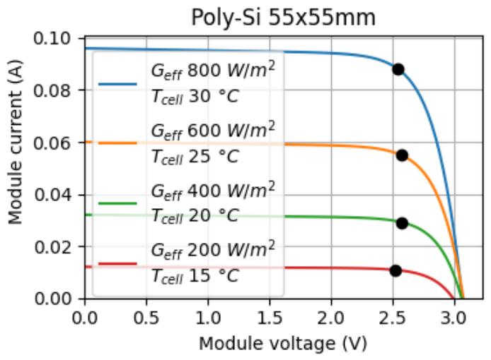
The resulting dataset, shown in Figure 7, represents the expected irradiance under ideal cloud-free conditions for the same timestamps as the measured current. In contrast to the measured data, the clear-sky GHI exhibits smooth and continuous profiles governed by solar geometry and atmospheric assumptions. In addition, PVLib was used to simulate the current–voltage (I–V) characteristics of the PV module under representative operating conditions as shown in Figure A2, providing an approximate reference for the expected current levels. This modeling step supports the interpretation of measured signals and ensures consistency between the observed PV response and theoretical behavior.
Figure 7.
Modeled clear-sky global horizontal irradiance (GHI) using the Ineichen–Perez model implemented in PVLib [49], corresponding to the timestamps of the available measured PV current. The smooth surface reflects ideal cloud-free conditions governed by solar geometry.
Figure 8, Figure 9 and Figure 10 illustrate the temporal availability of the recorded measurements using calendar-based visualizations. While some gaps are present due to acquisition interruptions, the dataset maintains sufficient seasonal coverage for subsequent analysis. In particular, the availability of PV current data is adequate for identifying clear-sky periods. Temperature and humidity measurements are included as complementary environmental variables, although they are not central to the clear-sky filtering procedure.
Figure 8.
Calendar plot of data availability for measured PV current. Colored cells indicate days with available data, while gaps correspond to missing or invalid measurements.
Figure 9.
Calendar plot of data availability for ambient temperature measured with the BME280 sensor (daily mean values) over 2024–2025. The color scale represents temperature magnitude, while gaps indicate missing data.
Figure 10.
Calendar plot of data availability for ambient relative humidity measured with the BME280 sensor (daily mean values) over 2024–2025. The color scale represents humidity levels, with gaps indicating missing data.
Overall the combination of measured PV current, environmental variables, and modeled clear-sky irradiance provides a consistent foundation for subsequent clear-sky detection and modeling.
3.2. Full Dataset with Time Encoding
To enrich the measured dataset and enable the model to capture temporal patterns, cyclical time features were introduced. Specifically, the hour of day and day of year were encoded using sine and cosine transformations, resulting in four additional inputs: sin(hour), cos(hour), sin(doy), and cos(doy) [51]. These features preserve the periodic nature of diurnal and seasonal cycles while avoiding discontinuities inherent to raw time indices. Figure 11 presents the resulting curated dataset, including measured PV current, environmental variables (temperature, humidity, and pressure), modeled clear-sky GHI, and solar zenith angle, together with the corresponding time encodings.
Figure 11.
Dataset of measured values and modeled Clear-Sky GHI, SZA, and time encoding.
3.3. Clear-Sky Modeling
To evaluate the impact of the tolerance parameter on both data availability and model performance, a sensitivity analysis was conducted for several tolerance levels , as summarized in Table 5. In addition, Table 6 reports the number of samples identified as clear-sky conditions for each tolerance, expressed as , together with the corresponding regression metrics.
Table 5.
Clear-sky sample counts with tolerance level grouped by zenith angle thresholds.
Table 6.
Clear-sky tolerance sensitivity. Sample count is reported as .
To assess the impact of angular-response effects, additional sensitivity analysis was performed using different solar zenith angle (SZA) thresholds (e.g., <75°, <80°, <83°, < 85°, < 90°). Stricter thresholds reduce the influence of high-incidence-angle conditions but also lead to a progressive reduction in the number of available clear-sky samples, observed in Table 5.
For example, at , the number of samples decreases from 36,233 for to 33,092 for and 29,170 for . While the reduction is moderate, it affects the statistical robustness and seasonal coverage of the dataset used for ANN training.
The selected threshold of therefore represents a trade-off between limiting angular-response errors and preserving sufficient data for stable model performance.
Increasing the tolerance parameter results in a larger number of identified clear-sky samples. However, this increase in sample size is accompanied by a gradual degradation in error metrics, reflecting the inclusion of less strictly matched conditions. For instance, the number of samples increases from 9622 at to 36,233 at , and further to over 61,000 at . However, this increase in sample size is accompanied by a gradual degradation in error metrics, such as nRMSE and nMAE, reflecting the inclusion of less strictly matched conditions.
A tolerance of was selected as a suitable compromise. At this level, a significantly larger dataset is retained compared to stricter thresholds (e.g., or ), which is beneficial for training data-driven models, while the performance metrics remain within acceptable limits. Moreover, the coefficient of determination R2 remains stable across the tested range, indicating that the overall predictive relationship is preserved.
Therefore, the choice of represents a practical trade-off between strict clear-sky filtering and sufficient data availability, ensuring both robustness and generalization capability in subsequent modeling tasks.
Table 6 summarizes the monthly and aggregated regression metrics, including slope, intercept, normalized RMSE (nRMSE), RMSE, MAE, and R2. The median slopes are consistently near 0.10–0.12, with intercepts generally small except for months with larger deviations. The total dataset exhibits an overall RMSE of 8.13 mA and MAE of 4.89 mA, with a strong coefficient of determination (R2 = 0.9052), confirming that the model effectively captures the underlying clear-sky PV current behavior while accommodating rare extreme errors.
From the clear-sky values identified in Figure 12, a representative scaling factor between modeled GHI_CS and PV current is obtained, and its stability across months is presented in Figure 13. Although Figure 12 illustrates the general approach used to identify clear-sky conditions, the actual selection was performed on a per-day basis using a min–max normalization technique to systematically extract all clear-sky samples. It should be noted that the signals shown in Figure 12 are normalized to their daily maximum values and are used only for clear-sky pattern identification, not for quantitative analysis.
Figure 12.
Clear-sky-like day detection using normalized signals. Both PV current () and modeled clear-sky irradiance () are normalized to their daily maximum values to enable shape-based comparison. Red points indicate samples within the selected solar zenith angle threshold (SZA < 83°), used for clear-sky identification.
Figure 13.
Stability of calibration coefficient.
The calibration coefficient shown in Figure 13 is computed exclusively from the clear-sky subset of the dataset, where the relationship between PV current and modeled clear-sky irradiance is expected to be physically consistent. Although the coefficient appears relatively stable across months, typically in the range of 0.10–0.11, it should not be interpreted as a strictly constant ratio. The observed variations, including the lower value in December, reflect seasonal changes in solar geometry, atmospheric conditions, and spectral effects. Furthermore, the values shown in Figure 13 represent monthly averages obtained through regression. At the instantaneous level, the ratio between PV current and clear-sky irradiance varies continuously as a function of solar zenith angle, temperature, and other environmental factors.
The ANN model is therefore introduced to capture this dynamic behavior, enabling a more accurate estimation of clear-sky PV current under varying conditions, rather than relying on a fixed or averaged calibration coefficient.
Figure 14 presents the linear relationship between measured PV current and modeled clear-sky irradiance for the selected clear-sky subset (, SZA ). The per-day min–max normalization and tolerance-based filtering ensure that only points closely following the daily irradiance shape are included, effectively isolating clear-sky conditions. The linear regression demonstrates a stable slope (≈0.10) across the dataset, confirming consistent scaling between panel current and irradiance. Performance metrics indicate a strong correlation, with R2 = 0.902 and acceptable error values (nRMSE = 0.173, RMSE = 8.25 mA, and MAE = 5.16 mA), highlighting that the filtered dataset reliably captures the underlying clear-sky PV behavior.
Figure 14.
Linear regression of clear-sky-like measured PV current (Current1) versus modeled clear-sky irradiance (GHI_CS) for the subset () and solar zenith angle SZA . The density-colored scatter plot shows the distribution of individual clear-sky-like points, while gray points represent data that do not meet the clear-sky selection criteria. The red line representing the fitted linear regression and the dashed line corresponding to a slope of 0.1 for reference. Statistical metrics including normalized RMSE (nRMSE), RMSE, MAE, and coefficient of determination (R2) are provided.
Figure 15 illustrates the relationship between measured PV current and the cosine of the solar zenith angle for the filtered clear-sky subset (, SZA ). Representing irradiance in terms of cos(SZA) accounts for the incidence angle effect on the module, offering a physically motivated perspective on current scaling. The linear regression slope remains consistent with the GHI-based analysis, while performance metrics (R2 = 0.892, nRMSE = 0.171, RMSE = 8.41 mA, MAE = 5.74 mA) confirm that the dataset reliably captures clear-sky behavior. Comparing the cos(SZA) representation with GHI demonstrates that both approaches yield similar scaling trends and support the tolerance choice as a practical balance between dataset purity and sample size. Figure 16 presents the distribution of absolute prediction error as a function of SZA.
Figure 15.
Linear regression of clear-sky-like measured PV current (Current1) versus cosine of the solar zenith angle (cos(SZA)) for and SZA . The density-colored scatter plot shows the distribution of points, with the red line representing the linear regression fit and the dashed line corresponding to a slope-based cosine reference. Gray points represent data that do not meet the clear-sky selection criteria. Key statistical metrics including the normalized RMSE (nRMSE), RMSE, MAE, and coefficient of determination (R2) are reported. Only points satisfying the per-day min–max normalized tolerance criterion are included.
Figure 16.
Distribution of absolute prediction error as a function of solar zenith angle (SZA) for the clear-sky-like subset (). Each boxplot represents the interquartile range (25th–75th percentile), with the median indicated by the central line and whiskers extending to 1.5 × IQR. Hollow circles indicate outliers beyond the whiskers. The results show a clear dependence of error magnitude on SZA, with larger errors occurring at higher zenith angles. This behavior reflects increased angular-response deviations and reduced signal quality under low solar elevation conditions.
Table 7 summarizes the monthly and aggregated regression metrics for the same clear-sky subset, including slope, intercept, normalized RMSE (nRMSE), RMSE, MAE, and coefficient of determination (R2). Consistent with the error distributions shown in Figure 17, most months exhibit high R2 values (>0.9) and small slopes around 0.10–0.12, indicating stable scaling between modeled clear-sky irradiance and measured current. Notably, months with larger median or extreme errors (e.g., December 2024, February 2025) correspond to lower R2 and higher RMSE/MAE, demonstrating that deviations in regression performance are largely driven by rare events rather than systematic model bias.
Table 7.
Monthly and aggregated clear-sky regression metrics ().
Figure 17.
Monthly distribution of absolute errors for the clear-sky-like subset of measured PV current ( = 5%). Each box represents the interquartile range (25th–75th percentile), with the median indicated by the central line. Whiskers extend to 1.5 × IQR, and crosses indicate outliers. Typical errors are small (<10 mA) for most months, while rare but extreme deviations occur, particularly in December 2024 and early 2025. These error patterns reflect seasonal variability in the regression performance of the clear-sky model.
Figure 17 presents the monthly distribution of absolute errors for the clear-sky-like subset of measured PV current, highlighting both typical and extreme deviations. For most months, the median errors are below 5 mA, indicating that the regression model closely captures the PV current under clear-sky conditions. Outliers, however, extend up to 70 mA, particularly in December 2024 and the early months of 2025, suggesting occasional larger deviations likely due to environmental factors or measurement variability.
To better understand the physical causes of prediction errors, the residuals of the clear-sky regression model were analyzed as a function of solar zenith angle (SZA). As shown in Figure 16, the absolute error exhibits a clear dependence on SZA. The largest absolute errors are observed in the intermediate SZA range (40–60°), corresponding to periods of higher irradiance and increased PV current. This behavior is primarily attributed to the scaling of absolute error with signal magnitude, rather than a degradation of model performance. At higher SZA values (>75°), the absolute error decreases due to reduced irradiance levels and lower signal amplitude. However, this does not necessarily imply improved relative accuracy under low-signal conditions.
Seasonal variations observed in Table 7 are consistent with this behavior, as winter months are associated with higher average SZA values and a reduced number of available clear-sky samples, which increases the statistical variability of the regression metrics. It should be noted that this analysis is based on a clear-sky-like subset of the dataset and therefore does not explicitly include cloud-induced variability.
The monthly clear-sky coverage is illustrated in Figure 18, showing both the total daytime minutes (modeled with PVlib, SZA ) and the subset of clear-sky minutes selected using the tolerance. The fraction of clear-sky minutes relative to total available daytime varies seasonally, from around 7% in December to over 21% in August, reflecting the combined effects of seasonal irradiance variability and local atmospheric conditions.
Figure 18.
Monthly clear-sky minutes. Gray bars show total daytime minutes (PVlib, SZA ), yellow bars indicate available daytime minutes in the measured dataset, and blue bars correspond to selected clear-sky minutes using tolerance. The percentages on the blue bars represent the fraction of clear-sky minutes relative to available daytime minutes.
Overall, the combined analysis of Figure 14, Figure 15, Figure 16 and Figure 17 and Table 7 confirms that the selected tolerance provides a robust balance between dataset size and regression accuracy, ensuring that the majority of clear-sky intervals are captured with high fidelity while accounting for occasional extreme deviations. The monthly metrics also provide insight into seasonal variability, which can inform subsequent modeling and PV system performance assessments.
3.4. Full Dataset Curated
Following the identification of clear-sky samples, the dataset was consolidated into a curated feature set suitable for subsequent modeling. This dataset combines measured PV current, environmental measurements (temperature, humidity, and pressure), modeled clear-sky irradiance (GHI_CS), solar zenith angle (SZA), and cyclical time encodings (hour and day of year expressed as sine and cosine components).
Figure 19 provides an overview of the complete dataset prior to filtering, where all variables are shown together over the full observation period. The representation highlights the heterogeneous nature of the inputs, including measured signals affected by atmospheric variability and deterministic features derived from solar geometry and time encoding.
Figure 19.
Overview of the initial dataset prior to clear-sky filtering, including measured PV current, environmental variables (temperature, humidity, pressure), modeled clear-sky irradiance (GHI_CS), solar zenith angle (SZA), and cyclical time encodings (hour and day of year). Each variable is represented by a distinct color for visualization purposes. All variables are normalized for visualization purposes.
Figure 18 presents the full dataset prior to filtering, highlighting the variability of measured signals under all sky conditions. After applying the clear-sky selection procedure, only samples consistent with clear-sky conditions were retained, as shown in Figure 19. This filtering step removes atmospheric disturbances such as cloud effects, resulting in smoother and physically consistent relationships between PV current and the modeled clear-sky irradiance.
After applying the clear-sky filtering procedure, only samples consistent with clear-sky conditions were retained. Figure 20 illustrates the resulting post-processed dataset, where non-clear-sky observations have been removed. For clarity, the day-of-year encodings are omitted from the visualization, while the remaining variables exhibit smoother and more consistent behavior. In particular, the PV current aligns more closely with the modeled clear-sky irradiance, confirming the effectiveness of the filtering approach.
Figure 20.
Post-processed dataset after clear-sky filtering. Non-clear-sky samples are removed, resulting in smoother and more consistent relationships between PV current and modeled clear-sky irradiance. Each variable is represented by a distinct color for visualization purposes. Day-of-year encodings are omitted for visualization clarity.
The curated clear-sky dataset is used to train an artificial neural network (ANN) to predict the clear-sky PV current () from time and environmental inputs. This predicted clear-sky current enables the estimation of the clear-sky index relationship as per Equation (8) as follows:
which can be rearranged to estimate GHI from measured PV current as follows (Equation (9)):
Thus, the ANN-derived clear-sky current serves as a key scaling factor, allowing the conversion of measured PV current into an estimate of global horizontal irradiance.
3.5. Machine Learning Analysis
To investigate the relationships between input variables and the clear-sky PV current, both statistical and model-based analyses were performed.
Figure 21 shows the Pearson correlation [52] matrix computed for the clear-sky dataset. As expected, the clear-sky PV current exhibits a strong negative correlation with solar zenith angle (SZA), reflecting the dominant role of solar geometry. Moderate correlations are observed with ambient temperature and relative humidity, while atmospheric pressure shows negligible influence. The time-encoding features (sine and cosine of hour and day of year) exhibit structured correlations with both SZA and the target variable, indicating redundancy but also complementary representations of periodic behavior.
Figure 21.
Pearson Correlation Matrix for the clear-sky dataset.
The ANN architecture was selected to balance predictive capability, generalization, and future deployment on resource-constrained embedded hardware. The model uses a compact feedforward structure with two hidden layers of sixteen and eight neurons, respectively, followed by a single linear output neuron for regression of clear-sky PV current. This funnel-shaped architecture is consistent with common design heuristics for small tabular datasets, where the number of hidden neurons is kept on the order of the input dimensionality and gradually reduced toward the output layer [53]. In the present case, the input space consists of time-related and environmental predictors, including clear-sky irradiance, solar zenith angle, temperature, humidity, pressure, and cyclical temporal encodings.
Two hidden layers were retained because they provide sufficient flexibility to approximate the smooth but nonlinear relationship between solar geometry, meteorological conditions, and PV current, while remaining shallow enough to limit overfitting. Compared with deeper networks, this architecture offers lower computational cost, fewer trainable parameters, and more stable behavior on a moderate-sized clear-sky dataset. The selected 16-8 configuration keeps the total parameter count below a few hundred, which is advantageous for later conversion to TensorFlow Lite Micro and deployment on a microcontroller.
The ANN was implemented as a feedforward neural network with two hidden layers of eight and six neurons, respectively, using hyperbolic tangent activation functions. The output layer consisted of a single linear neuron for regression of clear-sky PV current.
The model was trained using the Adam optimizer with mean squared error loss. A chronological split was used to avoid temporal leakage, with 70% of the dataset used for training and 30% for testing. A validation subset of 20% of the training data was used for early stopping.
Training was performed for up to 300 epochs with a batch size of 64 and early stopping based on validation loss (patience = 20, restore best weights enabled). Input features were standardized using statistics computed on the training set, and missing values were imputed using training-set medians. The configuration of the ANN model used for clear-sky PV current estimation is summarized in Table 8.
Table 8.
ANN model configuration for clear-sky PV current estimation.
Although larger architectures could potentially offer marginal improvements, they would increase memory footprint and inference cost without clear evidence of better generalization. Conversely, smaller alternatives such as a single hidden layer may be considered if stronger model compression is required, but the adopted two-layer structure was judged to provide the most suitable trade-off between representational capacity and deployability.
To interpret the ANN model, SHAP (SHapley Additive exPlanations) [54,55] values were computed. The summary plot in Figure 22 highlights the relative contribution of each feature to the model output. Solar zenith angle emerges as the most influential variable, followed by the cosine encoding of hour and the sine encoding of day of year. Environmental variables such as temperature and humidity have a comparatively smaller impact, with atmospheric pressure contributing negligibly.
Figure 22.
SHAP beeswarm.
The mean absolute SHAP values in Figure 23 further confirm this ranking, clearly showing the dominance of solar geometry and time-related features. Notably, relative humidity exhibits low importance and limited spread in SHAP values, indicating minimal contribution to the prediction of clear-sky current.
Figure 23.
SHAP mean feature importance.
Removing solar zenith angle from the input space leads to increased prediction error and a redistribution of feature importance toward cyclic time encodings, confirming the stabilizing role of explicit solar geometry.
To further assess the importance of solar zenith angle (SZA), a comparative analysis was conducted by training identical ANN models with and without SZA as an input feature. Figure 24 shows the monthly residual drift on the test block for both configurations.
Figure 24.
Monthly residual drift of ANN predictions on the test block for models with and without solar zenith angle (SZA). The inclusion of SZA significantly reduces bias and improves temporal stability across seasons.
The model including SZA exhibits residuals centered close to zero with relatively low variance across all months, indicating stable generalization over time. In contrast, the model without SZA shows a consistent negative bias and increased dispersion, particularly during winter and early spring months. This behavior suggests that time encodings alone are insufficient to fully capture the geometric effects of solar position.
These results confirm that, although SZA is theoretically derivable from time and location, its explicit inclusion as a feature significantly improves model stability and reduces temporal drift. This supports the decision to retain SZA in the final model despite its partial redundancy with time-based encodings.
While SHAP analysis indicates that solar zenith angle (SZA) is a dominant feature, it does not directly quantify model robustness. To address this, two additional analyses were performed.
First, a feature ablation study was conducted by removing SZA from the ANN input. This resulted in a significant degradation in performance, with RMSE increasing by 39.4% and R2 decreasing from 0.662 to 0.343, confirming that SZA is an important feature (Table 9).
Table 9.
Robustness analysis with respect to solar zenith angle (SZA).
Second, a Monte Carlo perturbation analysis was performed by introducing Gaussian noise () to the SZA input during evaluation. The resulting performance degradation was minimal (RMSE increase of 0.38%), with low variability across runs, indicating that the model is robust to moderate inaccuracies in solar geometry.
Furthermore, SHAP analysis of the reduced model (without SZA) shows that the dominant contribution shifts toward temporal encoding features, particularly the cosine of hour-of-day, indicating partial compensation when solar geometry is unavailable.
This behavior is reflected in Figure 24, where the removal of SZA introduces a systematic negative bias and increased variability, particularly during winter months.
3.6. Validation Against Reference Pyranometer (Cluj-Napoca)
To validate the proposed pseudo-pyranometer approach, an independent measurement experiment was conducted in Cluj-Napoca, Romania, where a calibrated reference pyranometer was available. While the primary dataset was collected in Piatra-Neamț, no co-located reference irradiance measurements were accessible at that site. Due to logistical constraints and equipment availability, the validation phase was therefore performed separately by temporarily relocating the measurement system.
The PV sensing system was deployed alongside the reference pyranometer ensuring synchronized acquisition under similar environmental conditions. This setup enables a direct comparison between the hybrid-ANN-derived irradiance estimates and ground-truth measurements.
To further evaluate the proposed method, a multi-day validation was performed under different sky conditions, including partially cloudy and cloudy days. The performance of the following three approaches was compared and is shown in Table 10: a purely physical model based on a constant calibration coefficient, a purely machine learning (ML) model, and the proposed hybrid method.
Table 10.
Performance comparison under partially cloudy and cloudy conditions.
Figure 25 and Figure 26 show representative examples for partially cloudy and cloudy conditions. The physical model exhibits large deviations, particularly during rapid irradiance fluctuations, while both the ML and hybrid models closely follow the measured GHI.
Figure 25.
Comparison of measured GHI and estimated GHI under partially cloudy conditions (5 April 2025). The hybrid model provides the most consistent agreement with measured GHI, particularly during transient cloud-induced variability.
Figure 26.
Comparison of measured GHI and estimated GHI under cloudy conditions (17 April 2025). The physical model exhibits large deviations and overestimation, while the ML and hybrid models closely track rapid irradiance fluctuations.
Quantitative results confirm this behavior, with the hybrid model achieving the lowest error across conditions. These results demonstrate that the hybrid approach effectively combines physical consistency with data-driven adaptability, providing robust performance under varying atmospheric conditions.
The constant-ratio model, defined as , yields RMSE = 149.23 W/m2 and MAE = 96.93 W/m2. In contrast, the purely data-driven ML model reduces the error to RMSE = 78.03 W/m2 and MAE = 52.50 W/m2, while the proposed hybrid model further improves performance to RMSE = 56.66 W/m2 and MAE = 39.26 W/m2 (Table 11).
Table 11.
Aggregate performance over the full validation dataset (Cluj-Napoca).
These results confirm that while the constant ratio assumption is valid under clear-sky conditions, it fails to capture the variability introduced by atmospheric effects. The ANN is therefore required to model the dynamic relationship between PV current and clear-sky response, leading to significantly improved accuracy under real-world conditions.
A potential limitation of evaluating only the reconstructed GHI is that errors in the ANN-predicted clear-sky current may be masked by compensation effects. To address this, an independent validation of the ANN was performed on the Cluj-Napoca dataset.
Clear-sky periods were identified using the same normalization-based detection approach applied during training. Under these conditions, the measured PV current can be considered a proxy for the true clear-sky current, enabling a direct comparison with the ANN infered .
The results (Figure 27) show a strong linear relationship between measured and predicted clear-sky current, with stable regression metrics across days. This confirms that the ANN generalizes well to the independent site without retraining.
Figure 27.
Clear-sky day detection using normalized signals for the analyzed dataset. Both PV current () and modeled clear-sky irradiance () are normalized to their daily maximum values to enable shape-based comparison. Red points indicate samples within the selected solar zenith angle threshold (SZA < 83°), used for clear-sky identification.
These findings demonstrate that the accurate GHI reconstruction is not the result of error compensation, but rather reflects the correct estimation of the underlying clear-sky PV response.
Figure 28 shows the relationship between the estimated GHI and the measured GHI from the pyranometer. A strong linear fit is observed, with a coefficient of determination R2 , indicating that the proposed method successfully captures the dominant irradiance dynamics. The normalized root mean square error (nRMSE = 0.179) and RMSE (56.66 W/m2) are within acceptable ranges for low-cost irradiance estimation approaches. A slight negative mean bias error (MBE = −9.70 W/m2) suggests a minor systematic underestimation.
Figure 28.
Comparison between estimated GHI (Equation (8)) and measured GHI from a reference pyranometer in Cluj-Napoca. The density scatter plot highlights strong agreement and near-linear behavior across the irradiance range.
The linear fit () further confirms the near-unity scaling between predicted and measured values, indicating that the ANN-based estimation combined with the clear-sky normalization preserves the physical proportionality between PV current and irradiance.
Figure 29 presents the residuals as a function of the estimated irradiance. The residual distribution is centered around zero for low to moderate irradiance levels, with increased dispersion observed at higher irradiance values. This behavior is consistent with increased variability in PV response and atmospheric conditions at high irradiance levels, as well as potential limitations of the clear-sky model under non-ideal conditions.
Figure 29.
Residuals between estimated GHI (Equation (8)) and measured GHI as a function of predicted irradiance. Increased dispersion at higher irradiance levels reflects higher variability and model limitations under strong solar conditions.
The relatively symmetric spread of residuals indicates that the model does not exhibit significant systematic errors across the dataset, while the dispersion reflects the combined effects of measurement noise, model approximation, and deviations from ideal clear-sky conditions. A slight skewness and the presence of outliers at higher residual magnitudes can be observed, which are likely associated with transient atmospheric effects or limitations in the clear-sky assumption.
Overall, the residual distribution confirms that the proposed approach provides unbiased and statistically consistent irradiance estimates, with errors largely confined within an acceptable range for low-cost sensing applications.
Figure 30 presents the distribution of residuals between the ANN-estimated irradiance and the reference pyranometer measurements. The residuals are approximately centered around zero, confirming the low bias previously indicated by the mean bias error (MBE = −9.70 W/m2). The distribution exhibits a near-Gaussian shape, with a fitted mean W/m2 and standard deviation W/m2, which is consistent with the reported RMSE.
Figure 30.
Histogram of residuals between hybrid-ANN-estimated-GHI and reference pyranometer measurements, with Gaussian fit. The black vertical dashed line indicates zero residual, while the red dashed curve represents the fitted Gaussian distribution. The distribution is centered near zero and exhibits an approximately normal shape, indicating low bias and consistent error characteristics.
Overall, the validation results demonstrate that the proposed pseudo-pyranometer approach provides reliable irradiance estimates, with good agreement against a reference instrument, despite being trained on data from a slightly different geographical location.
Site Transferability and Generalization
An important aspect of the proposed approach is its ability to generalize across different locations. As summarized in Table 3, both Piatra-Neamț and Cluj-Napoca are situated at similar latitudes (46.95° and 46.77°, respectively) and elevations (357 m vs. 370 m), and they share the same Köppen-Geiger climate classification (Dfb). These similarities imply comparable solar geometry and seasonal irradiance patterns, supporting the assumption that a model trained on clear-sky data from one site can be effectively transferred to the other.
The strong agreement observed during the Cluj-Napoca validation confirms this transferability, indicating that the learned relationship between PV current, solar geometry, and environmental variables remains consistent across sites with similar climatic conditions. This suggests that the proposed pseudo-pyranometer approach is not strictly site-dependent, provided that the geographical and climatic context is comparable.
Furthermore, beyond standalone irradiance estimation, the method has potential for practical deployment as a complementary calibration or correction tool for existing pyranometer measurements. In particular, the hybrid-ANN-based clear-sky current estimation combined with the clear-sky irradiance model could be used to detect drift, bias, or soiling effects in physical pyranometers, offering a low-cost and redundant validation mechanism in long-term monitoring systems.
4. Discussion
Results indicate that the hybrid modeling approach reliably captures the clear-sky current envelope and enables stable irradiance reconstruction using low-cost PV measurements. Feature importance analysis confirms that temporal encoding and solar geometry dominate the prediction of clear-sky current, while meteorological variables provide secondary refinement. The tolerance-based clear-sky selection method offers a practical compromise between sample size and modeling accuracy, enabling robust ANN training without requiring ground-truth irradiance measurements.
Validation against reference pyranometer observations demonstrates that the reconstructed GHI closely follows measured irradiance trends with consistent performance across seasons. This confirms the capability of the proposed approach to support distributed irradiance monitoring in scenarios where traditional instrumentation is unavailable. Validation is limited to two sites within the same Köppen–Geiger climate class (Dfb). While this allows assessment of cross-site transferability under similar climatic conditions, the model has not been evaluated in substantially different environments due to the lack of additional located measurements. Extending validation to diverse climatic regimes is left for future work.
Under clear-sky conditions, the relationship between PV current and modeled clear-sky irradiance is approximately linear, as shown in Figure 14 and Table 6. This suggests that a constant-ratio model of the form can provide a reasonable approximation under ideal conditions. To evaluate this hypothesis, a constant-ratio baseline was implemented using the mean calibration coefficient derived from clear-sky data. While this approach performs adequately under stable conditions, it fails to capture the variability introduced by atmospheric effects. A multi-day validation under partially cloudy and cloudy conditions shows that the constant-ratio model exhibits significantly higher errors compared to both the ML and hybrid approaches. For example, under cloudy conditions, the physical model yields RMSE = 268.17 W/m2, compared to 69.64 W/m2 for the ML model and 73.56 W/m2 for the hybrid model.
These results demonstrate that the constant-ratio assumption is insufficient under realistic conditions, and that the ANN is required to model the dynamic relationship between PV current and clear-sky response. This highlights that the ANN does not replace the physical relationship, but extends it by modeling its variability under non-ideal conditions. Rev 3.2.
Beyond the modeling framework, the proposed system was also briefly evaluated from a deployment perspective. As illustrated in Appendix A (Figure A3 and Figure A4), the sensing platform was reconstructed in a portable fashion, integrating the same current measurement, environmental sensing modules, along with auxiliary ones. In particular, the LSM303D sensor provides tilt estimation, ensuring that the PV panel remains close to horizontal alignment, which is critical for accurate GHI approximation. The DS3231 real-time clock (RTC) module provides precise timekeeping required for solar position estimation and clear-sky modeling. In this setup, to reduce computational overhead and enable embedded deployment, the clear-sky irradiance () was not computed using the full PVLib pipeline in real time. Instead, it was approximated using a solar-geometry-based formulation derived from the solar zenith angle [56] which can be efficiently computed on-device. This simplification allows real-time operation on microcontrollers while preserving the essential physical relationship between irradiance and solar position.
Furthermore, the trained ANN model was successfully ported to the embedded platform (Arduino Nano 33 BLE), demonstrating the feasibility of executing the hybrid physical-machine learning pipeline directly on low-power hardware. This enables a fully self-contained pseudo-pyranometer capable of real-time global horizontal irradiance estimation without reliance on external computation.
5. Conclusions
This study presents a hybrid physics-guided soft sensor for global horizontal irradiance estimation based on low-cost photovoltaic measurements and explainable neural-network modeling. By combining clear-sky irradiance modeling with ANN-based prediction of clear-sky panel current, the proposed framework enables reliable GHI estimation without direct radiometric sensors. Experimental validation shows that the approach provides consistent performance across seasonal conditions and can be replicated using inexpensive hardware. The method is therefore suitable for scalable solar monitoring networks, microgrid applications, and resource assessment in data-sparse regions. Future work will focus on multi-site deployments and adaptive online calibration to further improve long-term accuracy.
Author Contributions
Conceptualization, I.-V.V. and D.P.; methodology, I.-V.V.; software, I.-V.V.; validation, I.-V.V. and D.P.; formal analysis, I.-V.V.; investigation, I.-V.V.; resources, I.-V.V. and D.P.; data curation, I.-V.V.; writing-original draft preparation, I.-V.V.; writing-review and editing, I.-V.V. and D.P.; visualization, I.-V.V.; supervision, D.P. All authors have read and agreed to the published version of the manuscript.
Funding
This research is funded by the European Regional Development Fund (ERDF) through the Smart Growth, Digitalization and Financial Instruments Program, Contract No. 390085/11.11.2025, Project title: Ro-Green—Sustainable Electric Mobility Solutions, SMIS 336225.
Institutional Review Board Statement
Not applicable.
Informed Consent Statement
Not applicable.
Data Availability Statement
The raw photovoltaic current and environmental measurements used in this study are publicly available on Zenodo: V. Voicu, Raw photovoltaic current measurements from low-cost poly-Si and mono-Si panels with Raspberry Pi-based sensing (2024–2025), Zenodo, 2025. DOI: https://doi.org/10.5281/zenodo.17945957 [48].
Acknowledgments
The authors would like to thank Voicu Liviu for his valuable assistance with the mechanical aspects of the installation and setup of the measurement system in Piatra-Neamț.
Conflicts of Interest
The authors declare no conflicts of interest.
Abbreviations
The following abbreviations are used in this manuscript:
| AMSL | Above Mean Sea Level |
| ANN | Artificial Neural Network |
| GHI | Global Horizontal Irradiance |
| HAT | Hardware Attached on Top |
| IQR | Interquartile Range |
| ML | Machine Learning |
| Mono-Si | Monocrystalline Silicon |
| POA | Plane-of-Array |
| PoE | Power-over-Ethernet |
| Poly-Si | Polycrystalline Silicon |
| PV | Photovoltaic |
Appendix A
Appendix A.1
Figure A1.
Data acquisition system components: Raspberry Pi 5, INA219 Current Hat with 0.3 W PV panel, PoE HAT, BME280, and Raspberry Pi HQ Camera. Arrows indicate physical and electrical connections between components.
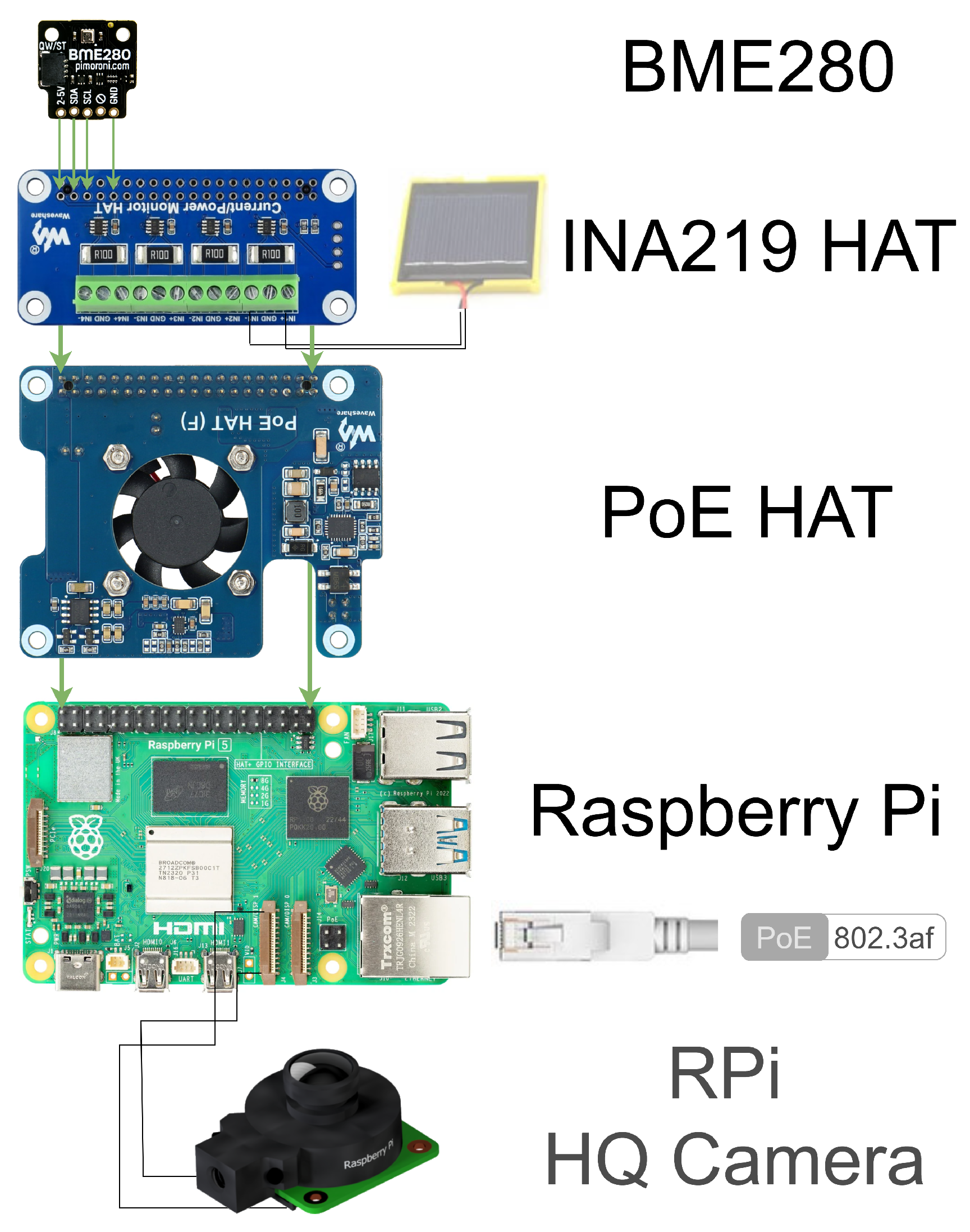
Table A1.
Approximate cost of hardware components used in the proposed system.
Figure A2.
Modeled current–voltage (I–V) characteristics of a 55 × 55 mm poly-Si PV module using PVlib [57]. Curves show the module current as a function of voltage under varying effective irradiance (200–800 W/m2) and cell temperature (15–30 °C). Black markers indicate the maximum power points for each condition.
Appendix A.2
Figure A3.
Portable implementation of the proposed pseudo-pyranometer on an Arduino Nano 33 BLE platform, integrating sensing, timekeeping, and processing components required for embedded irradiance estimation. The system integrates (1) an LSM303D sensor mounted in the plane of the PV panel for tilt estimation, ensuring near-horizontal alignment, with measurements rejected when tilt exceeds 3°; (2) an OLED display for real-time visualization, (3) an INA219 current sensor for PV current measurement, (4) a DS3231 real-time clock (RTC) for precise timekeeping, and (5) a BME280 sensor for environmental measurements.
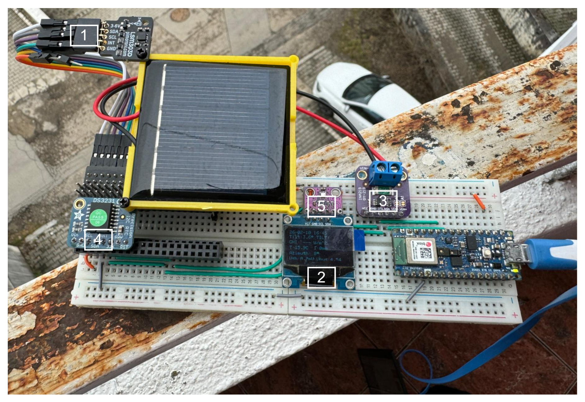
Figure A4.
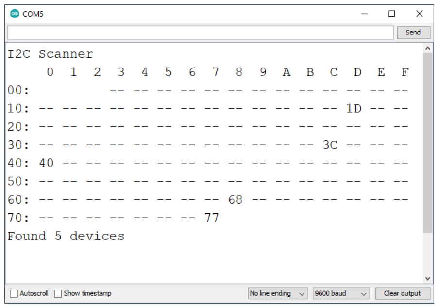
I2C bus scan of the embedded system showing the detected addresses of connected sensors and modules. Detected device addresses are displayed in hexadecimal format, while “–” indicates that no device is present at the corresponding address. The scan confirms correct integration and communication of all peripherals used in the portable pseudo-pyranometer platform.
References
- Dunn, L.; Gostein, M.; Emery, K. Comparison of pyranometers vs. PV reference cells for evaluation of PV array performance. In Proceedings of the 2012 38th IEEE Photovoltaic Specialists Conference; IEEE: Piscataway, NJ, USA, 2012; pp. 002899–002904. [Google Scholar] [CrossRef] [Scilit]
- Chenlo, F.; Vela, N.; Olivares, J. Comparison between pyranometers and encapsulated solar cells as reference PV sensors-outdoor measurements in real conditions. In Proceedings of the IEEE Conference on Photovoltaic Specialists; IEEE: Piscataway, NJ, USA, 1990; Volume 2, pp. 1099–1104. [Google Scholar] [CrossRef] [Scilit]
- Meydbray, J.; Emery, K.; Kurtz, S. Pyranometers and Reference Cells, What’s the Difference? National Renewable Energy Laboratory (NREL): Golden, CO, USA, 2012. [Google Scholar]
- Gouvêa, E.C.; Sobrinho, P.M.; Souza, T.M. Spectral Response of Polycrystalline Silicon Photovoltaic Cells under Real-Use Conditions. Energies 2017, 10, 1178. [Google Scholar] [CrossRef] [Scilit]
- Azouzoute, A.; Merrouni, A.A.; Bennouna, E.G.; Gennioui, A. Accuracy Measurement of Pyranometer vs Reference cell for PV resource assessment. Energy Procedia 2019, 157, 1202–1209. [Google Scholar] [CrossRef] [Scilit]
- Peterson, J.; Andreas, A.; Habte, A.; Sengupta, M. Equating Reference Cell and Broadband Pyranometer Data. In Proceedings of the 2024 IEEE 52nd Photovoltaic Specialist Conference (PVSC); IEEE: Piscataway, NJ, USA, 2024; pp. 1045–1052. [Google Scholar] [CrossRef] [Scilit]
- Mubarak, R.; Schilke, H.; Seckmeyer, G. Improving the Irradiance Data Measured by Silicon-Based Sensors. Energies 2021, 14, 2766. [Google Scholar] [CrossRef] [Scilit]
- Pvlib Developers. Pvlib Python. 2025. Available online: https://github.com/pvlib/pvlib-python (accessed on 1 December 2025).
- ISO 9060:2018; Solar Energy—Specification and Classification of Instruments for Measuring Hemispherical Solar and Direct Solar Radiation. International Organization for Standardization: Geneva, Switzerland, 2018.
- IEC 60904-2; Photovoltaic Devices—Part 2: Requirements for Photovoltaic Reference Devices. International Electrotechnical Commission: Geneva, Switzerland, 2023.
- Cheddadi, Y.; Cheddadi, H.; Cheddadi, F.; Errahimi, F.; Es-sbai, N. Design and implementation of an intelligent low-cost IoT solution for energy monitoring of photovoltaic stations. SN Appl. Sci. 2020, 2, 1165. [Google Scholar] [CrossRef] [Scilit]
- Fanourakis, S.; Wang, K.; McCarthy, P.; Jiao, L. Low-cost data acquisition systems for photovoltaic system monitoring and usage statistics. IOP Conf. Ser. Earth Environ. Sci. 2017, 93, 012048. [Google Scholar] [CrossRef] [Scilit]
- Rivera-Medina, R.D.J.; Ordaz-García, O.O.; García-Duran, A.; Ibarra-Delgado, S.; Sandoval-Aréchiga, R.; Gómez-Rodríguez, J.R.; Rodríguez-Abdalá, V.I.; Guerrero-Osuna, H.A. Real-Time Solar Irradiance Monitoring: An FPGA-Based Approach for Data Visualization. Appl. Sci. 2025, 15, 12407. [Google Scholar] [CrossRef] [Scilit]
- Martínez, M.A.; Andújar, J.M.; Enrique, J.M. A New and Inexpensive Pyranometer for the Visible Spectral Range. Sensors 2009, 9, 4615–4634. [Google Scholar] [CrossRef] [Scilit]
- Dantas, E.C.S.; Segundo, J.T.D.; Catunda, S.Y.C.; Belfort, D.R.; Freire, R.C.S.; Silva Júnior, P.F.d. Architecture of an Electrical Equivalence Pyranometer with Temperature Difference Analog Control. Sensors 2022, 22, 8137. [Google Scholar] [CrossRef] [Scilit]
- Oyelami, S.; Azeez, N.A.; Ologunye, O.B.; Adeyi, A.J.; Adegboye, T.A.; Olawale, O.K.; Olawuyi, O.A. Development of a low-cost wireless data logging Pyrano-meter with inbuilt temperature and humidity monitoring system. Environ. Chall. 2021, 5, 100219. [Google Scholar] [CrossRef] [Scilit]
- Lim, M.T.M.; Tan, R.H.G.; Tan, G.A.; Hew, C.H.; Lee, W.K.; Mercha, M. Development of low cost pyranometer IoT based solar irradiance measurement station. IOP Conf. Ser. Earth Environ. Sci. 2023, 1281, 012012. [Google Scholar] [CrossRef] [Scilit]
- Ronilaya, F.; Ramadhani, P.F.; Hidayat, M.N.; Wibowo, S.; Eryk, I.H.; Pratama, S.S.V.P. A Development of a Low Cost Solar Irradiance Meter Using Mini Solar Cells. In Proceedings of the 2022 International Conference on Informatics Electrical and Electronics (ICIEE); IEEE: Piscataway, NJ, USA, 2022; pp. 1–5. [Google Scholar] [CrossRef] [Scilit]
- Orsetti, C.; Muttillo, M.; Parente, F.; Pantoli, L.; Stornelli, V.; Ferri, G. Reliable and Inexpensive Solar Irradiance Measurement System Design. Procedia Eng. 2016, 168, 1767–1770. [Google Scholar] [CrossRef] [Scilit]
- Nespoli, L.; Medici, V. An unsupervised method for estimating the global horizontal irradiance from photovoltaic power measurements. Sol. Energy 2017, 158, 701–710. [Google Scholar] [CrossRef] [Scilit]
- Ma, J.; Bi, Z.; Shi, Y.; Man, K.L.; Pan, X.; Wang, J. OL-SVR based soft-sensor for real-time estimation of solar irradiance. In Proceedings of the 2016 IEEE Asia Pacific Conference on Circuits and Systems (APCCAS); IEEE: Piscataway, NJ, USA, 2016; pp. 448–451. [Google Scholar] [CrossRef] [Scilit]
- Hameed, W.I.; Sawadi, B.A.; Al-Kamil, S.J.; Al-Radhi, M.S.; Al-Yasir, Y.I.A.; Saleh, A.L.; Abd-Alhameed, R.A. Prediction of Solar Irradiance Based on Artificial Neural Networks. Inventions 2019, 4, 45. [Google Scholar] [CrossRef] [Scilit]
- Chouay, Y.; Ouassaid, M. An accurate real time neural network based irradiance and temperature sensor for photovoltaic applications. Results Eng. 2024, 21, 101766. [Google Scholar] [CrossRef] [Scilit]
- Nava-Pintor, J.A.; Alcalá-Rodríguez, U.E.; Guerrero-Osuna, H.A.; Mata-Romero, M.E.; Lopez-Neri, E.; García-Vázquez, F.; Solís-Sánchez, L.O.; Carrasco-Navarro, R.; Luque-Vega, L.F. Development and Evaluation of Solar Radiation Sensor Using Cost-Effective Light Sensors and Machine Learning Techniques. Technologies 2025, 13, 182. [Google Scholar] [CrossRef] [Scilit]
- Calizaya-Neira, C.R.; Coaquira-Castillo, R.J.; Utrilla Mego, L.W.; Herrera-Levano, J.C.; Palomino Lopez, A.; Moreno-Cardenas, E.; Sacoto-Cabrera, E.J. Prototype Design for Irradiance Estimation Using Closed-Form Models and an Optimized MPPT IC Algorithm. Electronics 2025, 14, 1652. [Google Scholar] [CrossRef] [Scilit]
- Duffie, J.A.; Beckman, W.A. Solar Engineering of Thermal Processes, 4th ed.; John Wiley & Sons, Inc.: Hoboken, NJ, USA, 2013. [Google Scholar] [CrossRef] [Scilit]
- Wenham, S.R.; Green, M.A.; Watt, M.E.; Corkish, R.; Sproul, A. (Eds.) Applied Photovoltaics, 3rd ed.; Routledge: London, UK, 2012. [Google Scholar] [CrossRef] [Scilit]
- Green, M.A. Solar Cells: Operating Principles, Technology, and System Applications; Prentice-Hall, Inc.: Englewood Cliffs, NJ, USA, 1982. [Google Scholar]
- Sze, S.M.; Ng, K.K. Physics of Semiconductor Devices, 3rd ed.; Wiley-Interscience: Hoboken, NJ, USA, 2006. [Google Scholar] [CrossRef] [Scilit]
- Boyd, M.T.; Hansen, C. Single Diode Equivalent Circuit Models. 2013. Available online: https://pvpmc.sandia.gov/modeling-guide/2-dc-module-iv/single-diode-equivalent-circuit-models/ (accessed on 1 December 2025).
- Peel, M.C.; Finlayson, B.L.; McMahon, T.A. Updated world map of the Köppen-Geiger climate classification. Hydrol. Earth Syst. Sci. 2007, 11, 1633–1644. [Google Scholar] [CrossRef] [Scilit]
- StatsClimat. Climate Statistics for Cluj-Napoca, Romania. Available online: https://statsclimat.com/Europe/Romania/report_ClujNapoca (accessed on 1 December 2025).
- Climate-Data.org. Climate Data for Cluj-Napoca, Romania. Available online: https://en.climate-data.org/europe/romania/cluj/cluj-napoca-764/ (accessed on 1 December 2025).
- StatsClimat. Climate Statistics for Piatra Neamț, Romania. Available online: https://statsclimat.com/Europe/Romania/report_Piatra_Neamt (accessed on 1 December 2025).
- Climate-Data.org. Climate Data for Piatra Neamț, Romania. Available online: https://en.climate-data.org/europe/romania/neamt/piatra-neamt-1354/ (accessed on 1 December 2025).
- Raspberry Pi Foundation Raspberry Pi 5. 2025. Available online: https://www.raspberrypi.com/products/raspberry-pi-5/ (accessed on 1 December 2025).
- Raspberry Pi. Raspberry Pi High Quality Camera. Available online: https://www.raspberrypi.com/products/raspberry-pi-high-quality-camera (accessed on 23 March 2026).
- Arducam. Arducam 180 Degree Fisheye 1/2.3″ M12 Lens with Lens Adapter for Raspberry Pi High Quality Camera. Available online: https://www.arducam.com/arducam-180-degree-fisheye-1-2-3-m12-mount-with-lens-adapter-for-raspberry-pi-high-quality-camera.html (accessed on 23 March 2026).
- Pimoroni. BME280 Breakout. 2023. Available online: https://shop.pimoroni.com/products/bme280-breakout?variant=29420960677971 (accessed on 1 December 2025).
- Waveshare. Current Power Monitor HAT. 2023. Available online: https://www.waveshare.com/current-power-monitor-hat.htm (accessed on 1 December 2025).
- Waveshare. PoE HAT for Raspberry Pi. 2023. Available online: https://www.waveshare.com/poe-hat-f.htm (accessed on 1 December 2025).
- Long, C.N.; Ackerman, T.P. Identification of clear skies from broadband pyranometer measurements and calculation of downwelling shortwave cloud effects. J. Geophys. Res. Atmos. 2000, 105, 15609–15626. [Google Scholar] [CrossRef] [Scilit]
- Reno, M.J.; Hansen, C.W. Identification of periods of clear sky irradiance in time series of GHI measurements. Renew. Energy 2016, 90, 520–531. [Google Scholar] [CrossRef] [Scilit]
- Ellis, B.H.; Deceglie, M.; Jain, A. Automatic Detection of Clear-Sky Periods From Irradiance Data. IEEE J. Photovolt. 2019, 9, 998–1005. [Google Scholar] [CrossRef] [Scilit]
- Wandji Nyamsi, W.; Lindfors, A. Detecting clear-sky periods from photovoltaic power measurements. Meteorol. Appl. 2024, 31, e2201. [Google Scholar] [CrossRef] [Scilit]
- Peratikou, S.; Charalambides, A.G. Estimating clear-sky PV electricity production without exogenous data. Sol. Energy Adv. 2022, 2, 100015. [Google Scholar] [CrossRef] [Scilit]
- Li, B.; Virtuani, A.; Ballif, C.; Faes, A.; Quest, H. An interpretable AI framework for clear-sky detection in photovoltaics monitoring. EPJ Photovolt. 2025, 16, 32. [Google Scholar] [CrossRef] [Scilit]
- Voicu, V. Raw photovoltaic current measurements from low- cost poly-Si and mono-Si panels with Raspberry Pi based sensing (2024 to 2025). Zenodo 2025. [Google Scholar] [CrossRef]
- Anderson, K.S.; Hansen, C.W.; Holmgren, W.F.; Jensen, A.R.; Mikofski, M.A.; Driesse, A. pvlib python: 2023 project update. J. Open Source Softw. 2023, 8, 5994. [Google Scholar] [CrossRef] [Scilit]
- Ineichen, P.; Perez, R. A new airmass independent formulation for the Linke turbidity coefficient. Sol. Energy 2002, 73, 151–157. [Google Scholar] [CrossRef] [Scilit]
- NVIDIA. Three Approaches to Encoding Time Information as Features for ML Models, 2023. Available online: https://developer.nvidia.com/blog/three-approaches-to-encoding-time-information-as-features-for-ml-models/ (accessed on 1 December 2025).
- Pearson, K. Notes on regression and inheritance in the case of two parents. Proc. R. Soc. Lond. 1895, 58, 240–242. [Google Scholar] [CrossRef] [Scilit]
- Hagan, M.T. Neural Network Design, 2nd ed.; Oklahoma State University: Stillwater, OK, USA, 2014. [Google Scholar]
- Lundberg, S.; Lee, S.I. SHAP: SHapley Additive exPlanations. GitHub Repository, MIT License. Available online: https://github.com/shap/shap (accessed on 1 December 2025).
- Lundberg, S.M.; Lee, S.I. A Unified Approach to Interpreting Model Predictions. In Proceedings of the Advances in Neural Information Processing Systems 30; Curran Associates, Inc.: Red Hook, NY, USA, 2017; pp. 4765–4774. [Google Scholar]
- Reno, M.J.; Hansen, C.W.; Stein, J.S. Global Horizontal Irradiance Clear Sky Models: Implementation and Analysis; Technical Report SAND2012-2389; Sandia National Laboratories: Albuquerque, NM, USA; Livermore, CA, USA, 2012. [CrossRef] [Scilit]
- Holmgren, W.F.; Hansen, C.W.; Mikofski, M.A. pvlib python: A Python package for modeling solar energy systems. J. Open Source Softw. 2018, 3, 884. [Google Scholar] [CrossRef] [Scilit]
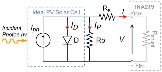
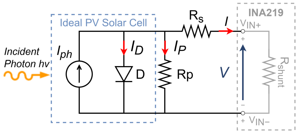
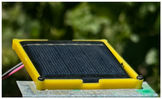
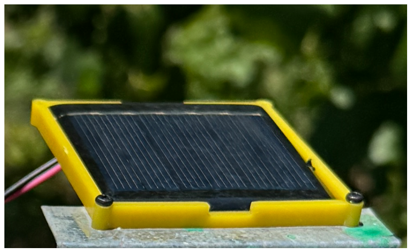
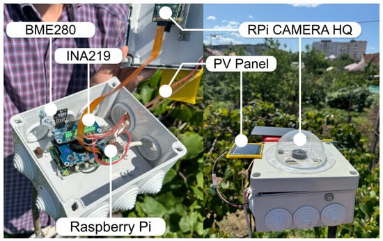
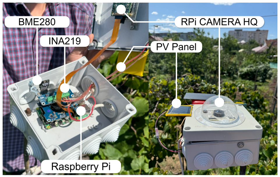
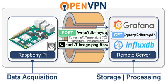
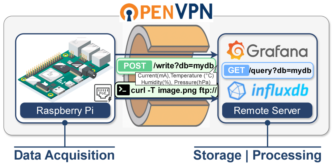
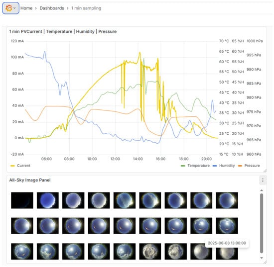
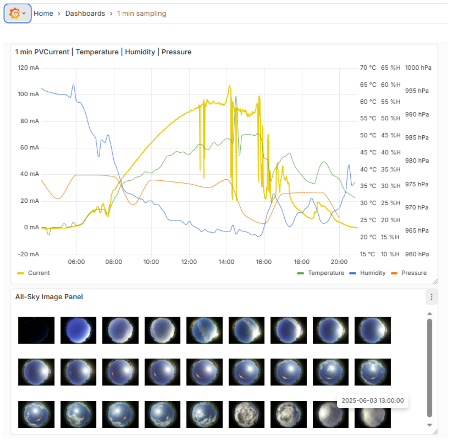
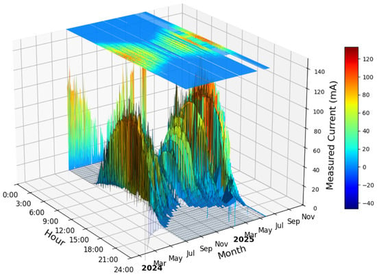
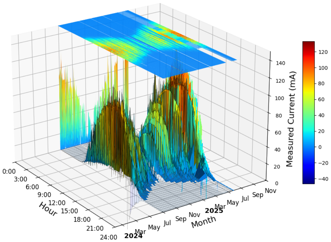
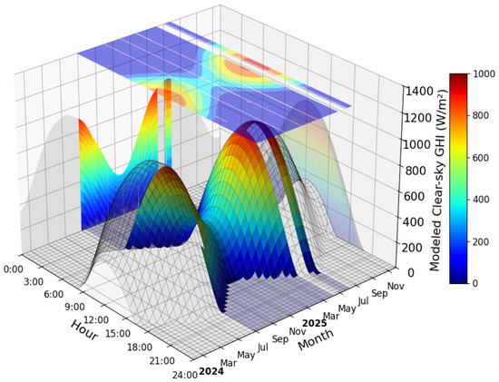
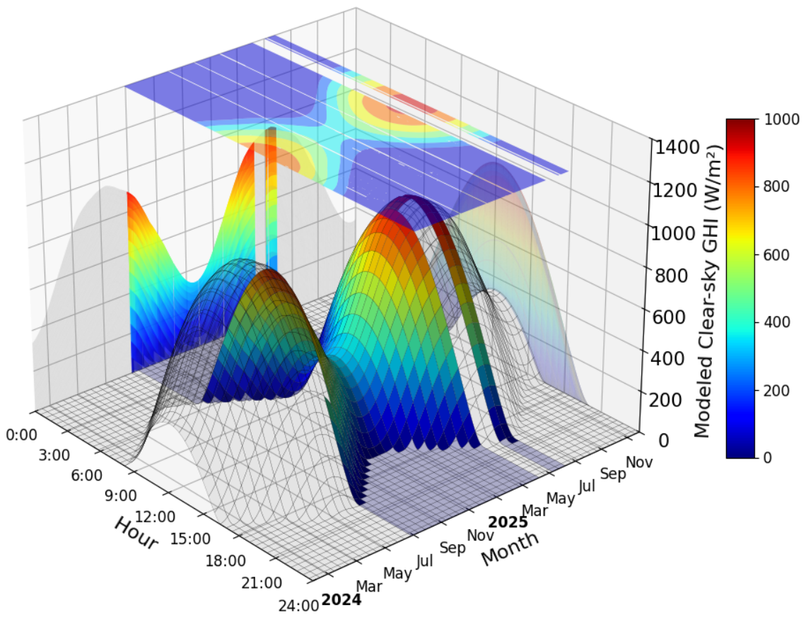
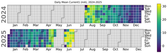
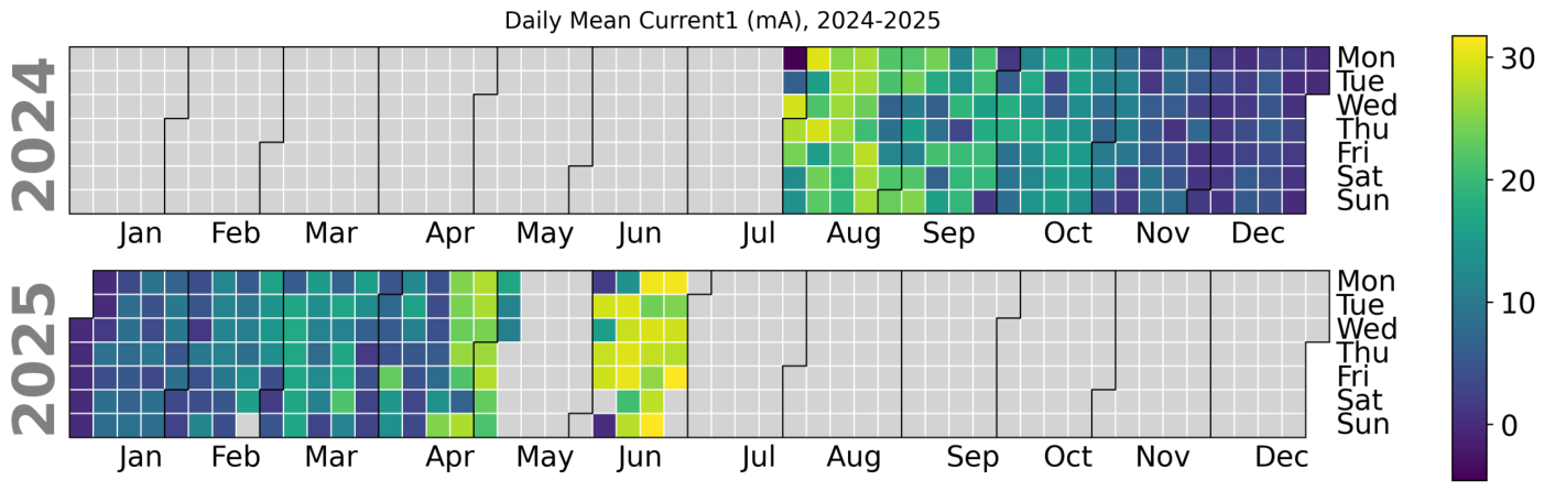
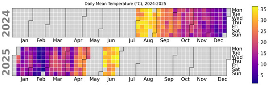
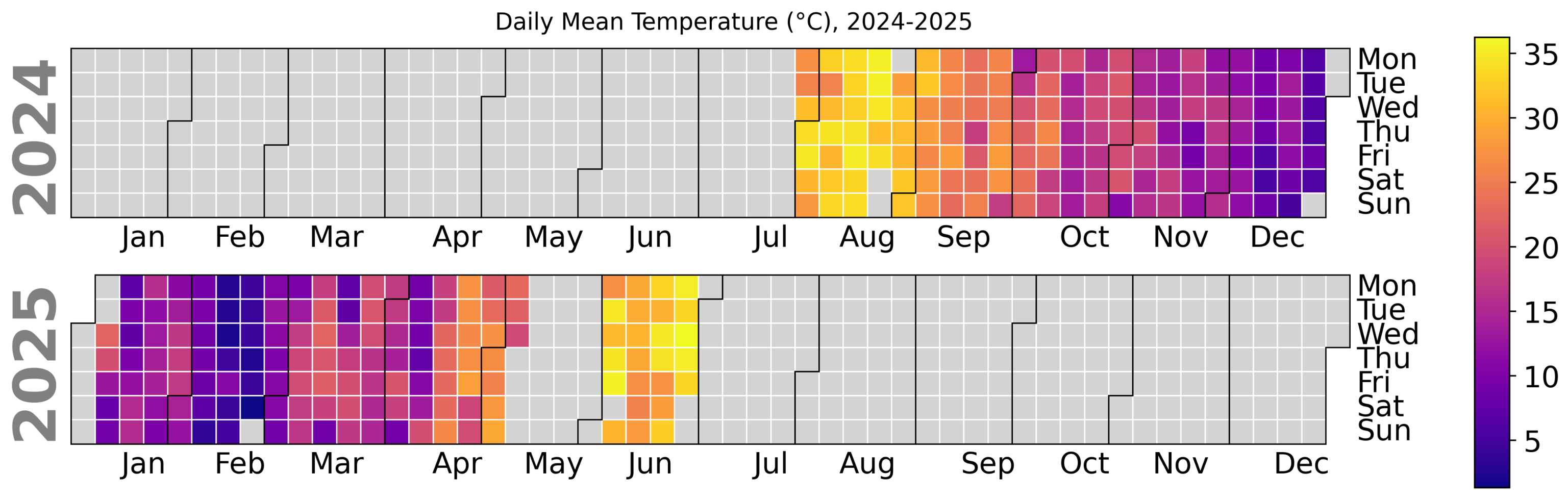
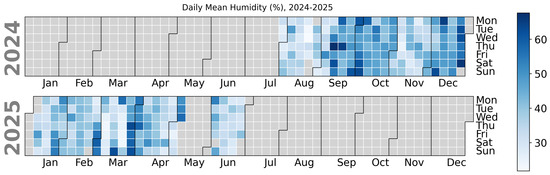
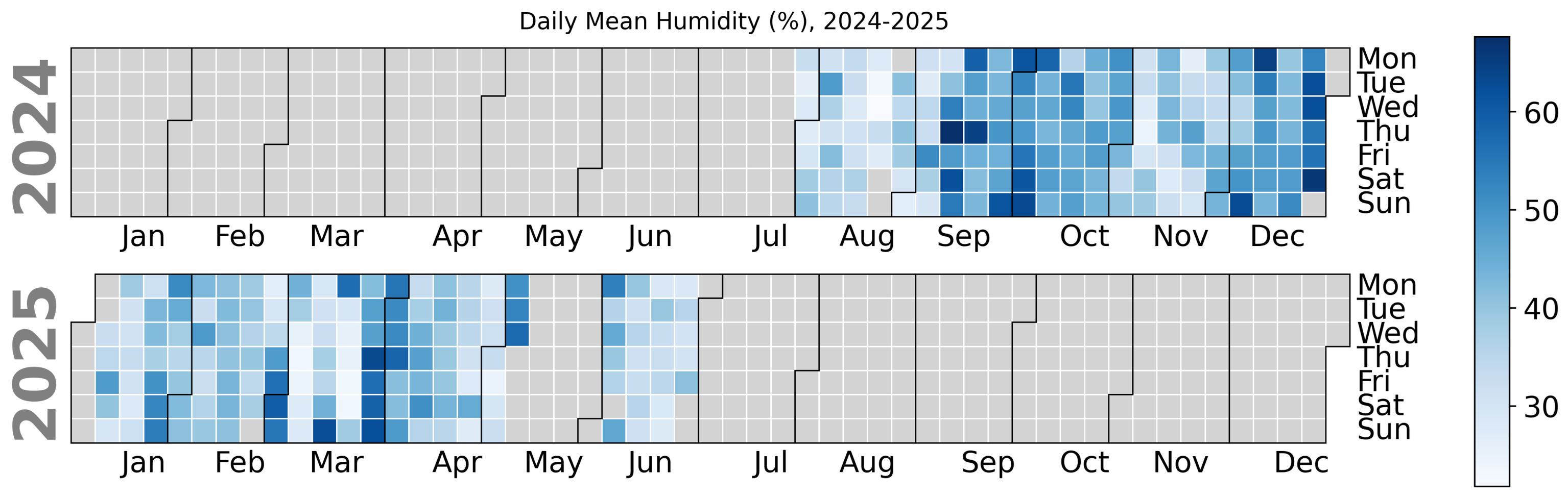
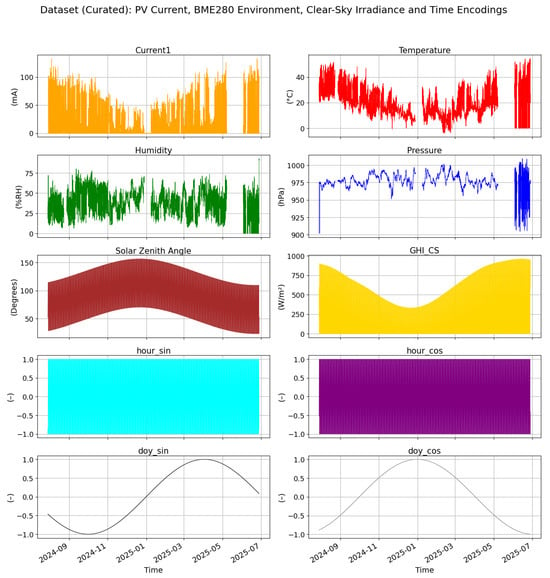
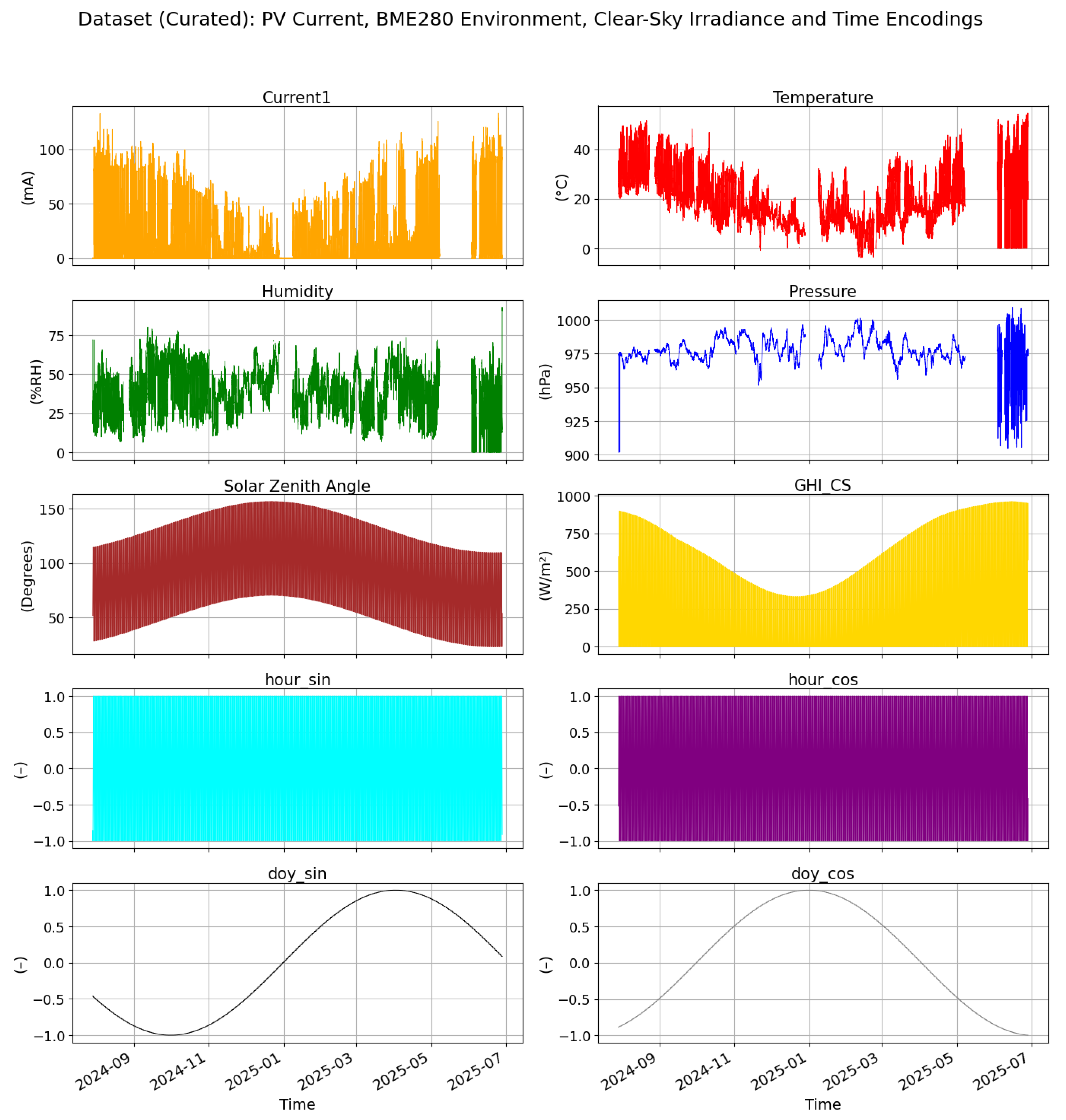
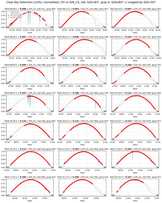
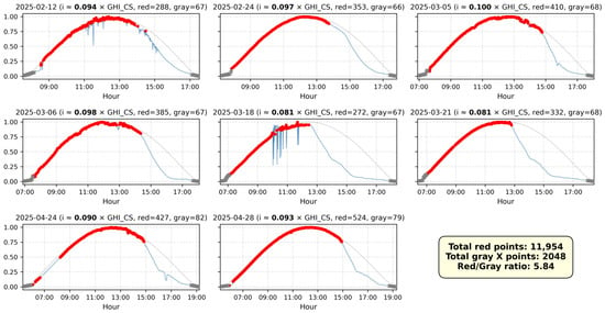
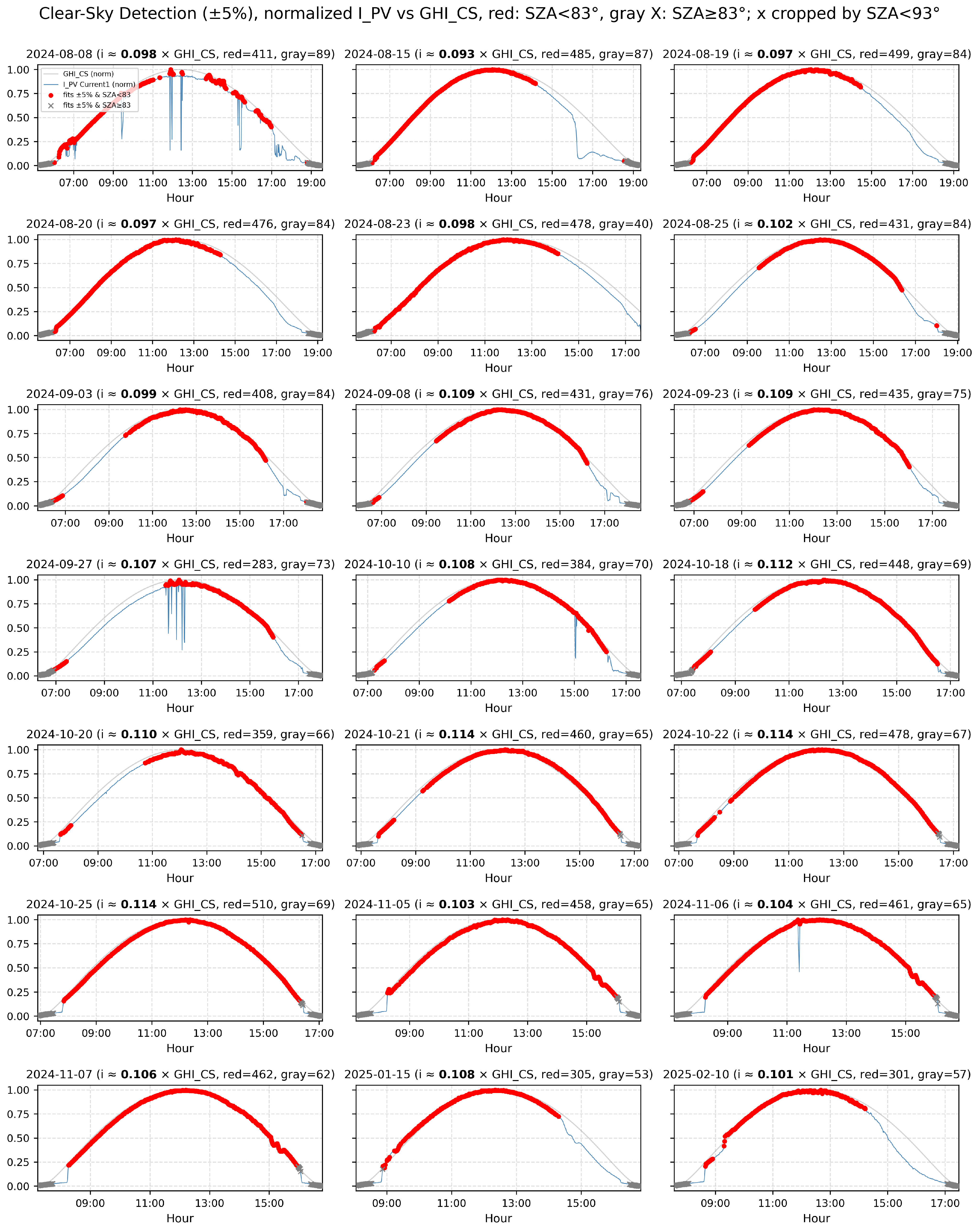
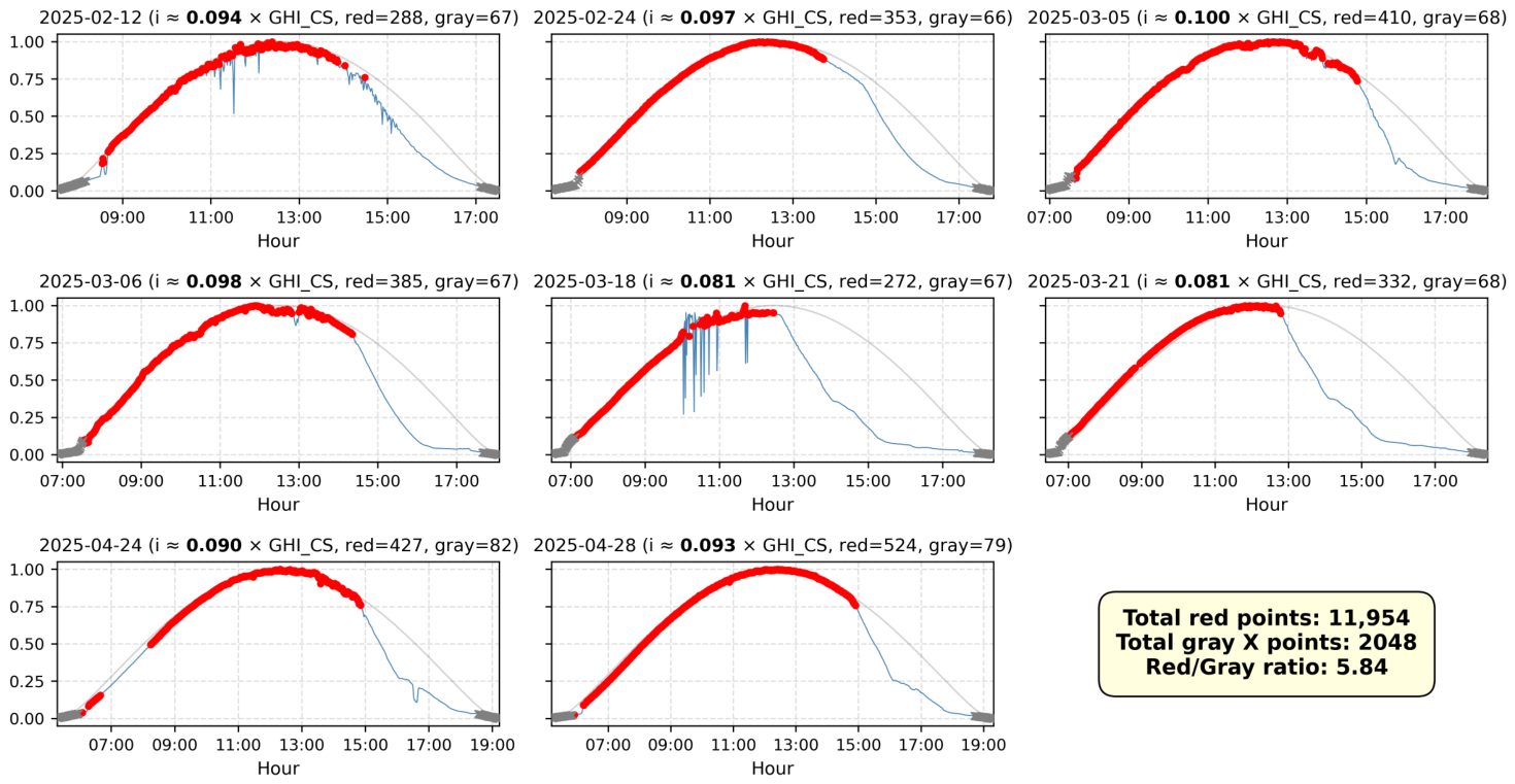
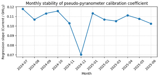
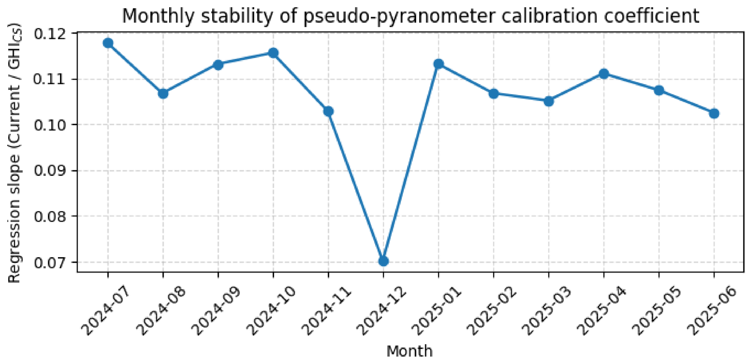
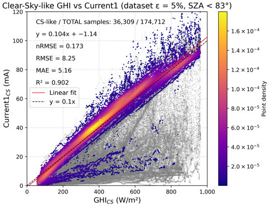
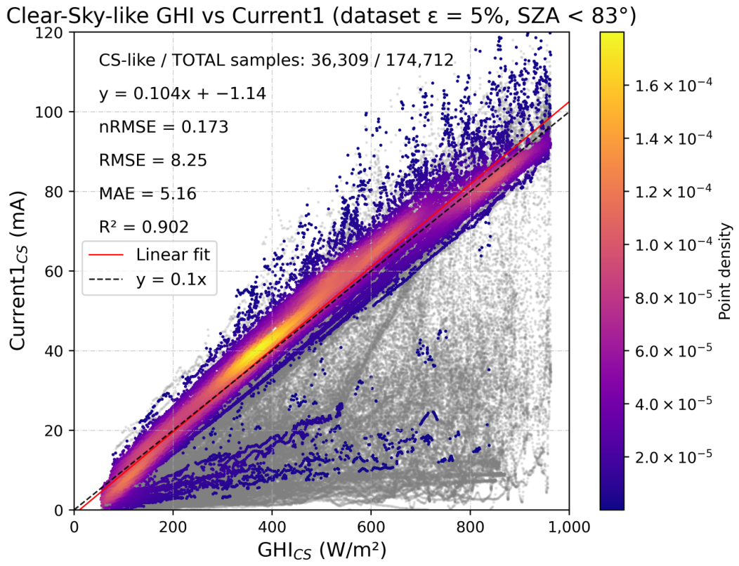
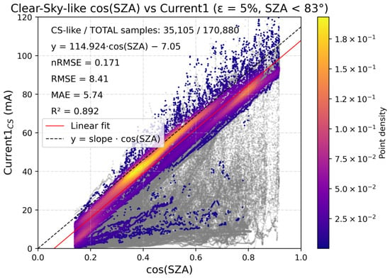
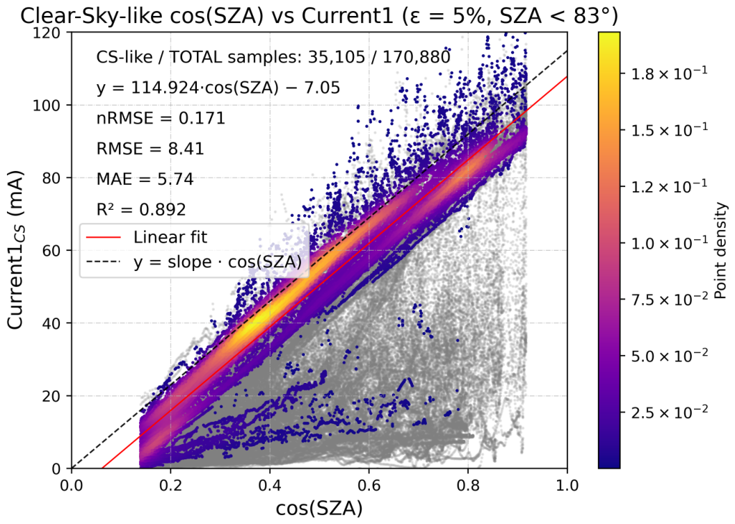
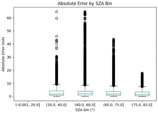
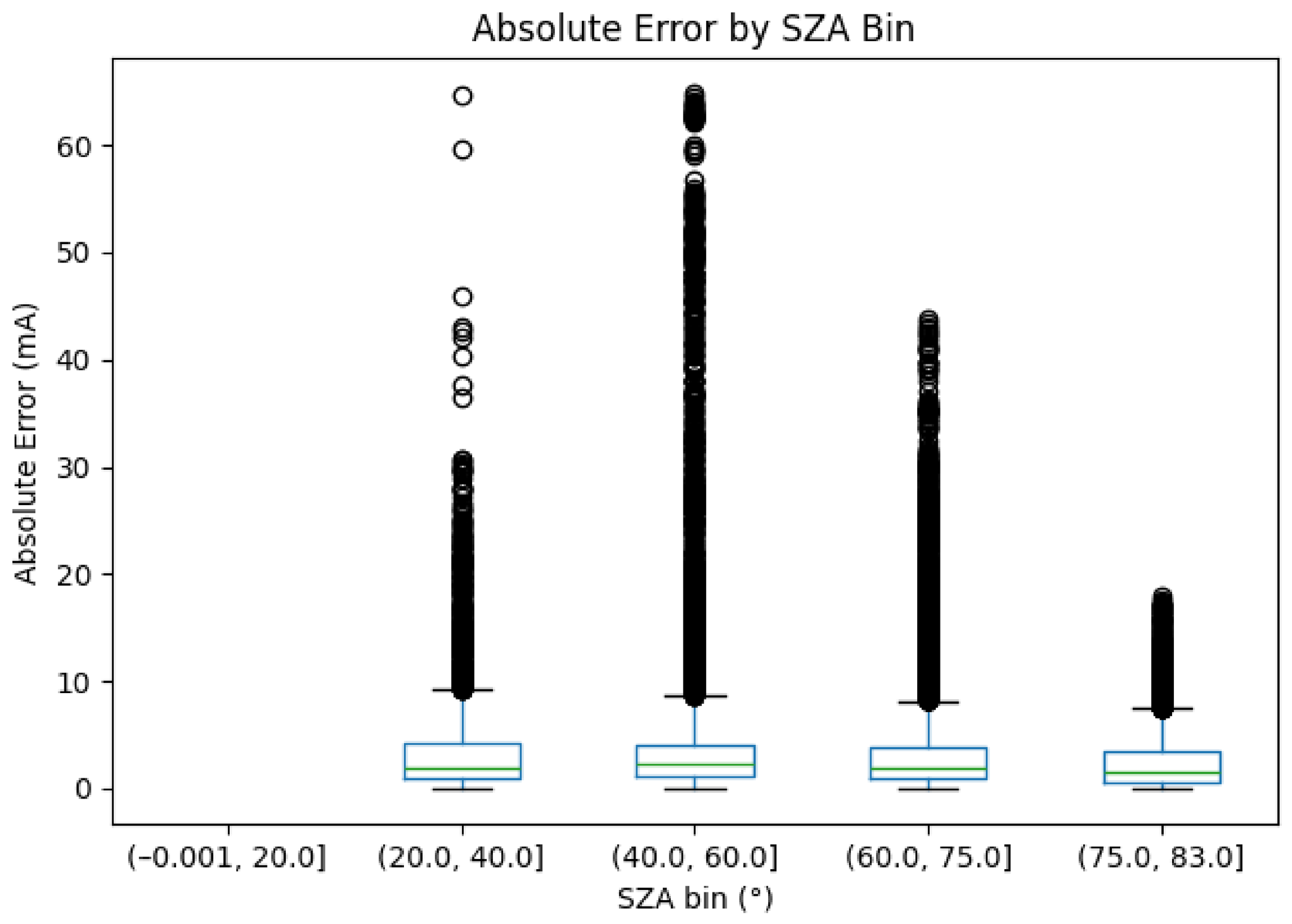
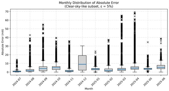
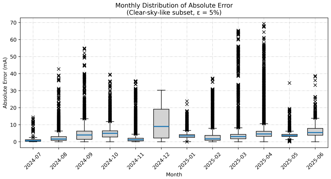
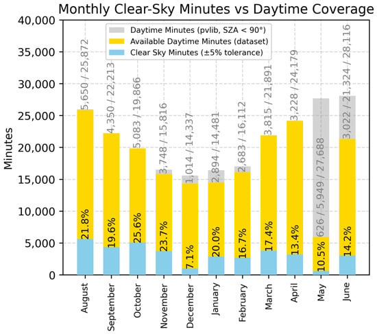
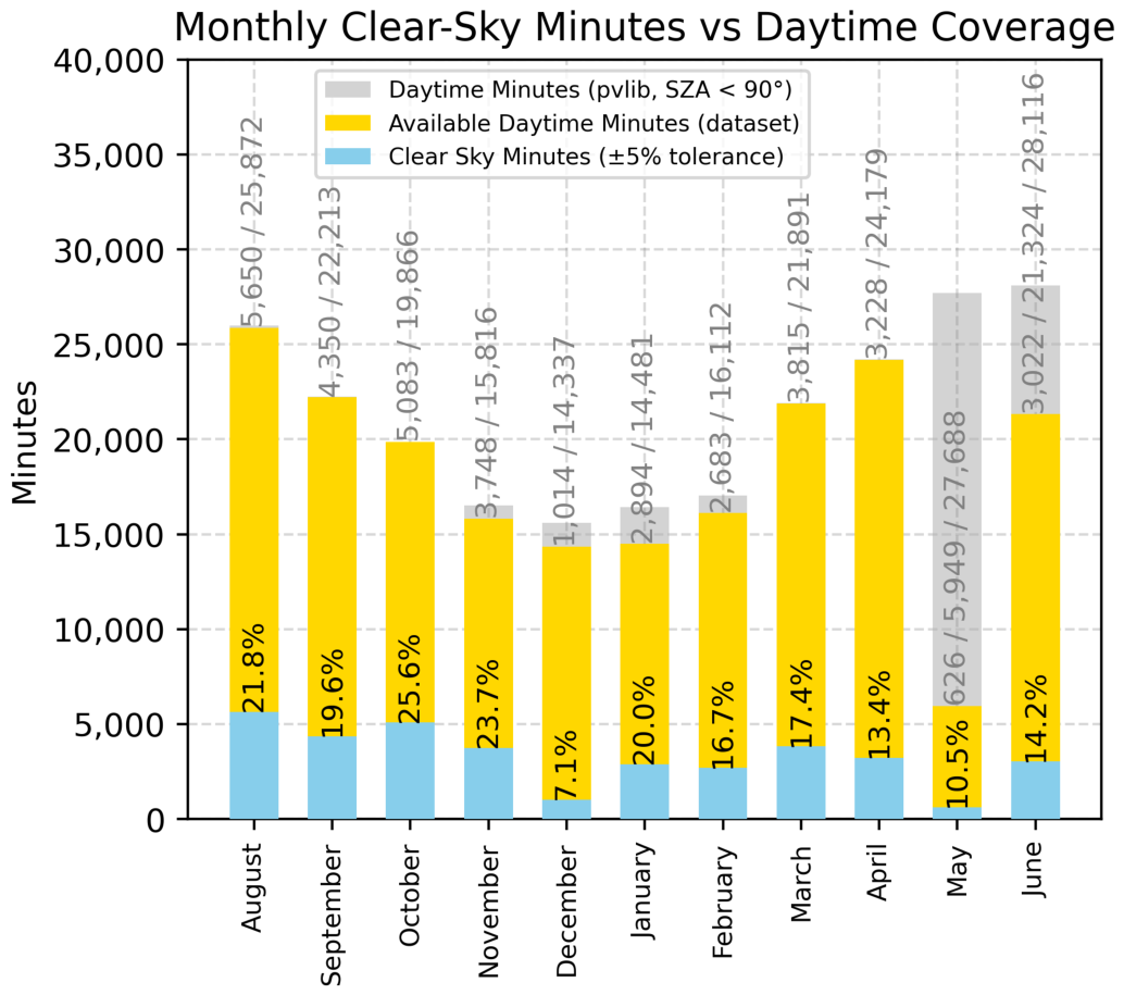
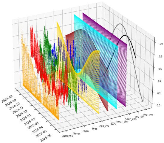
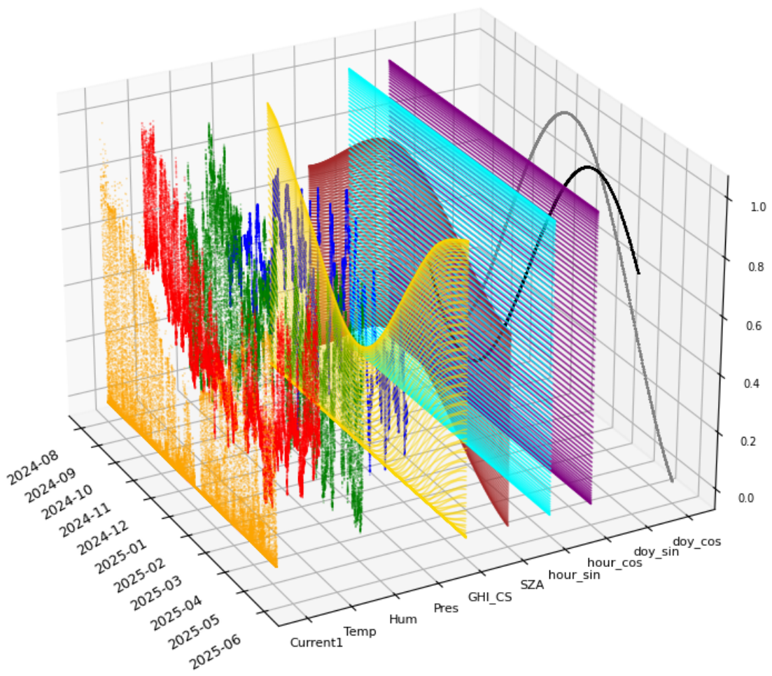
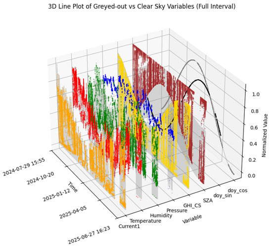
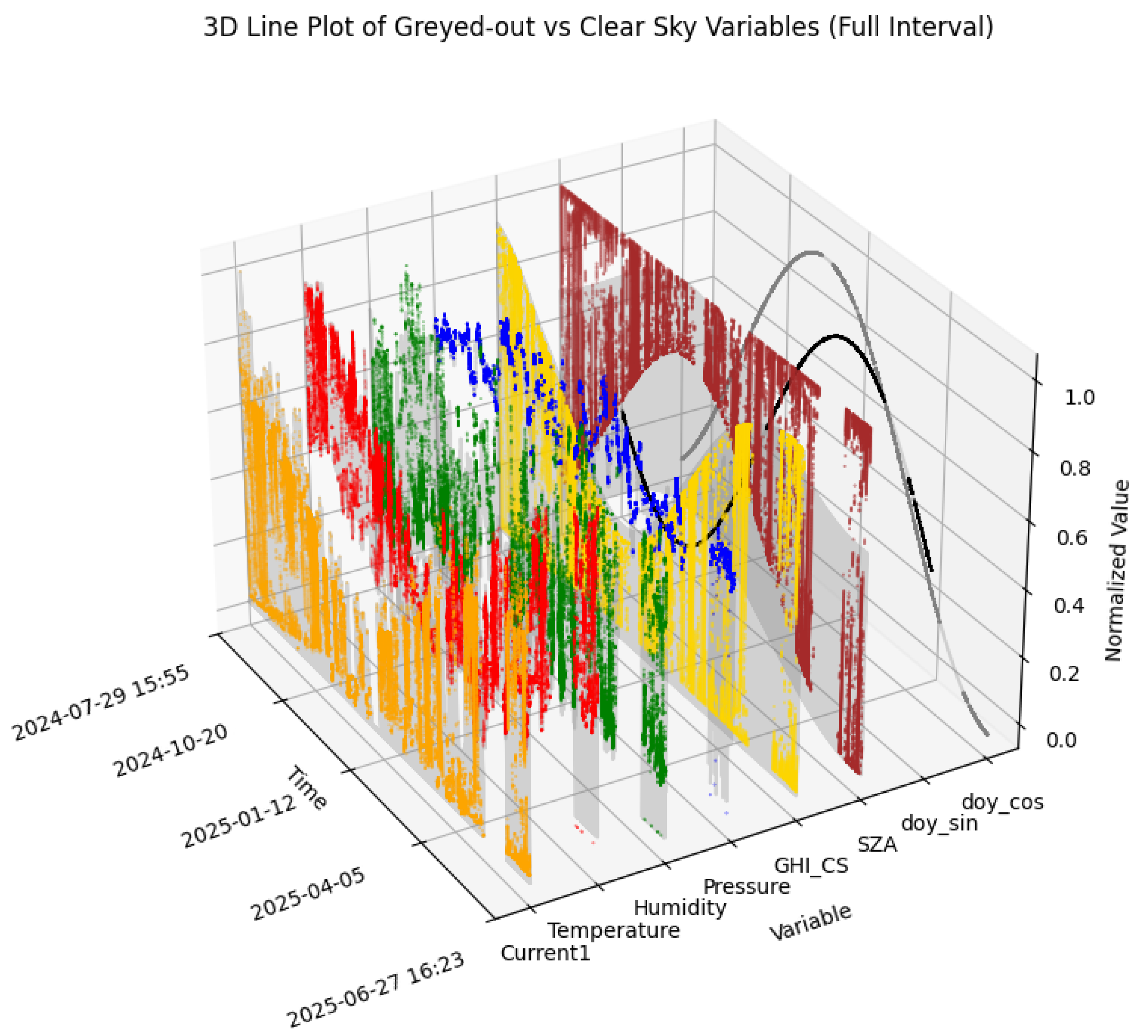
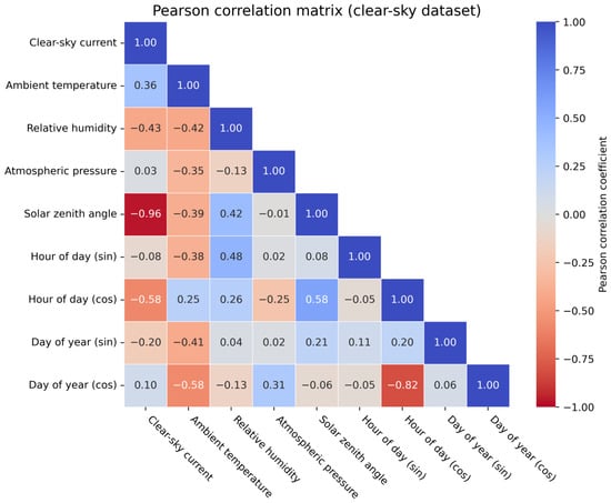
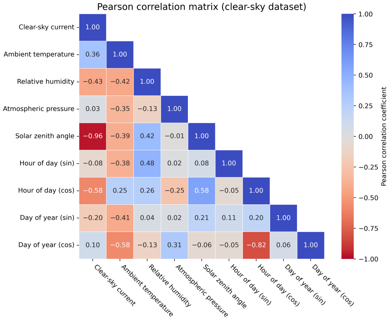
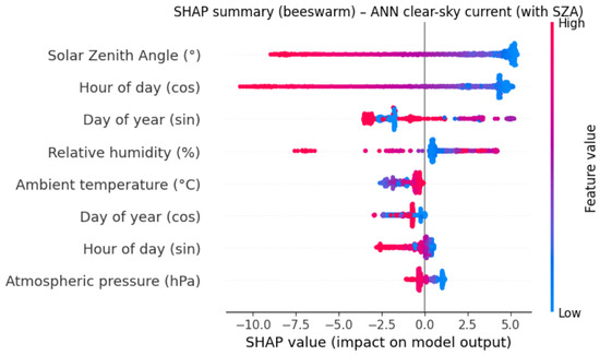
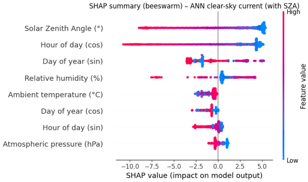
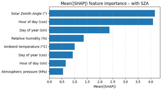
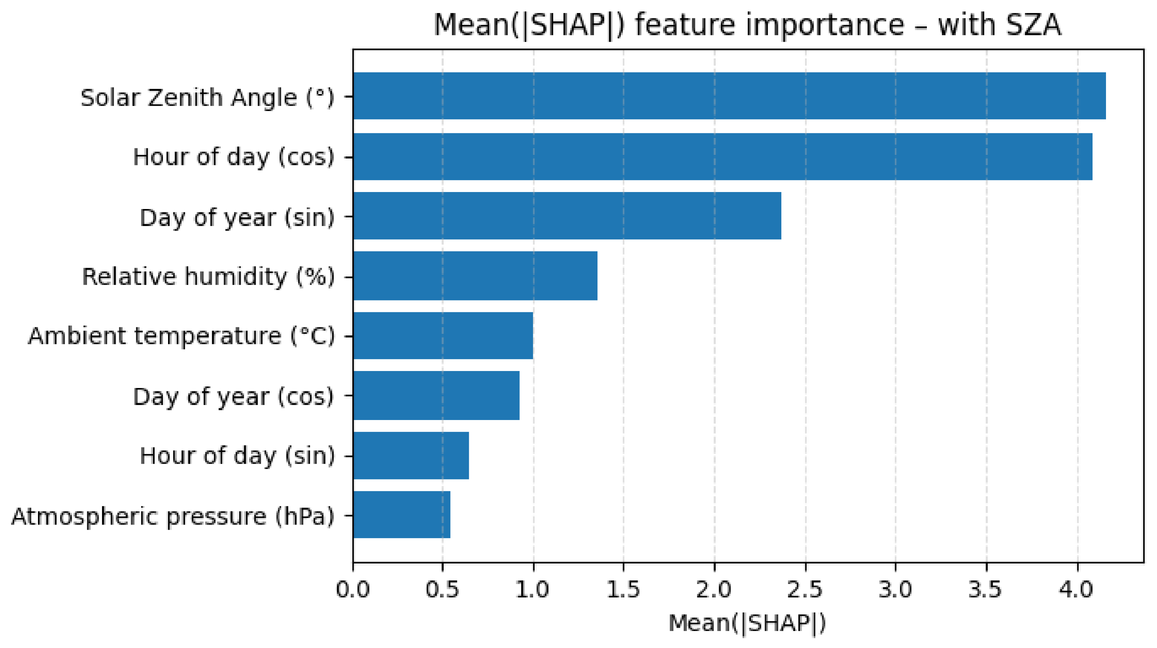
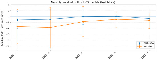
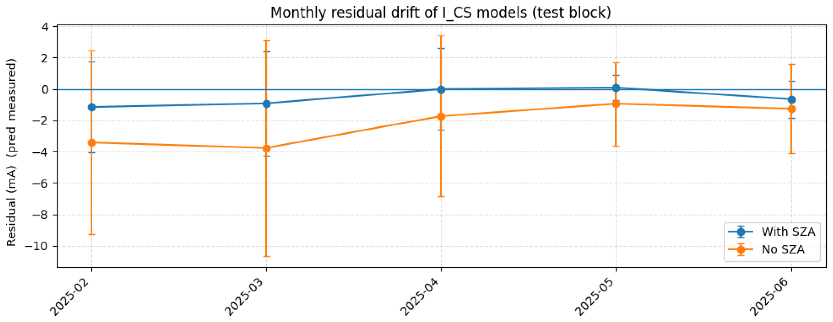
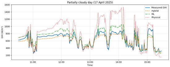
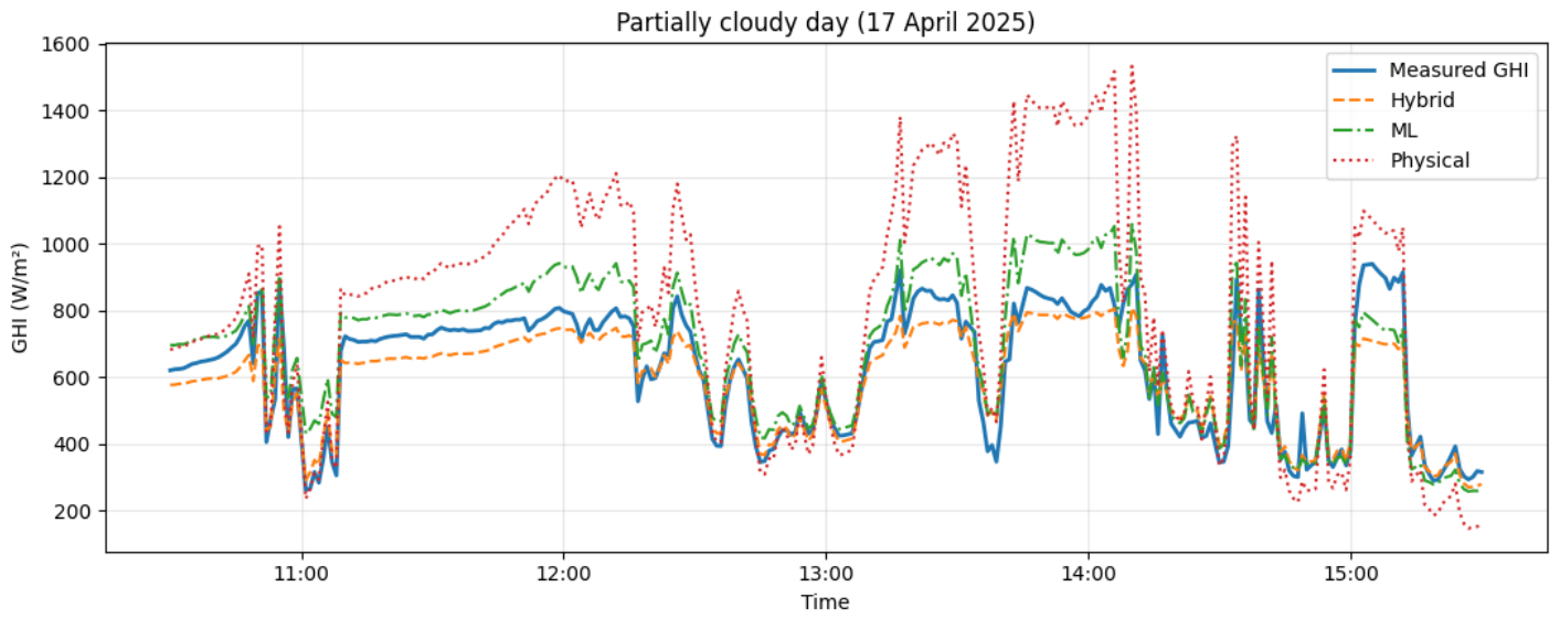
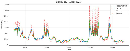
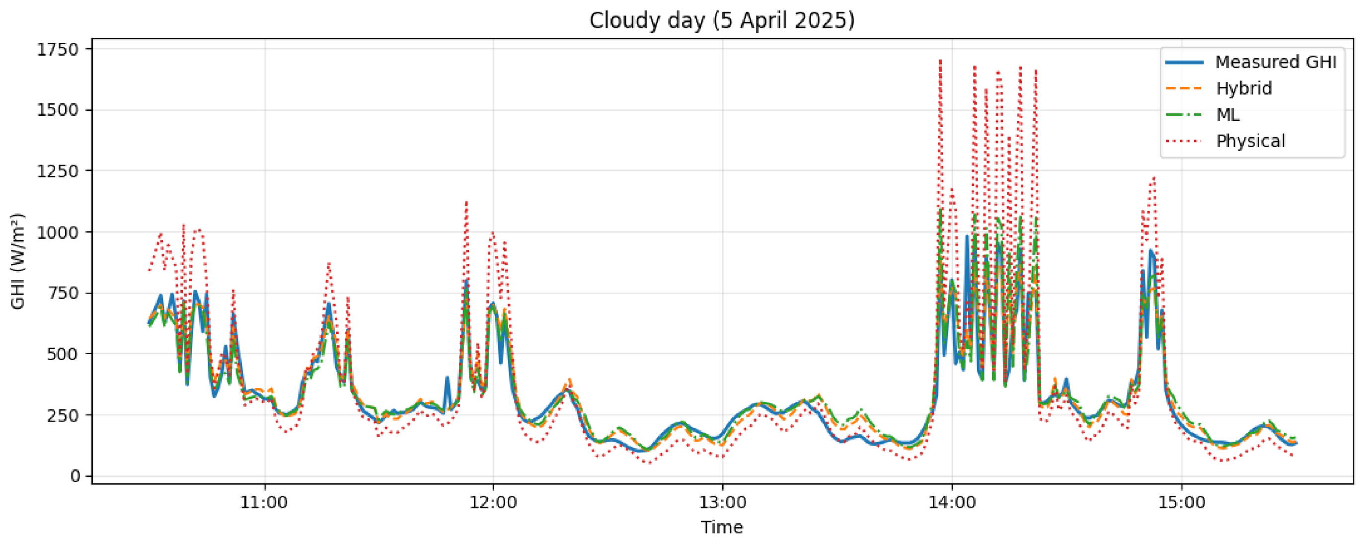
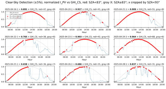
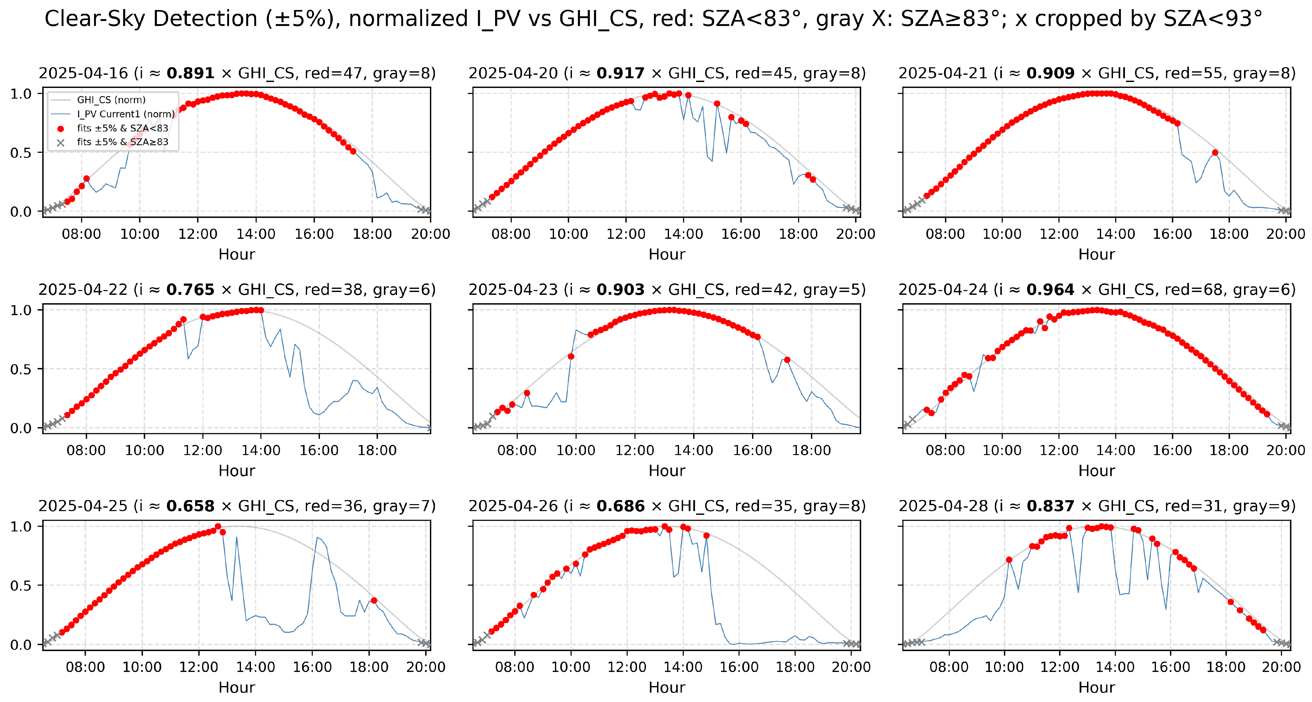
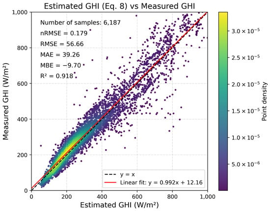
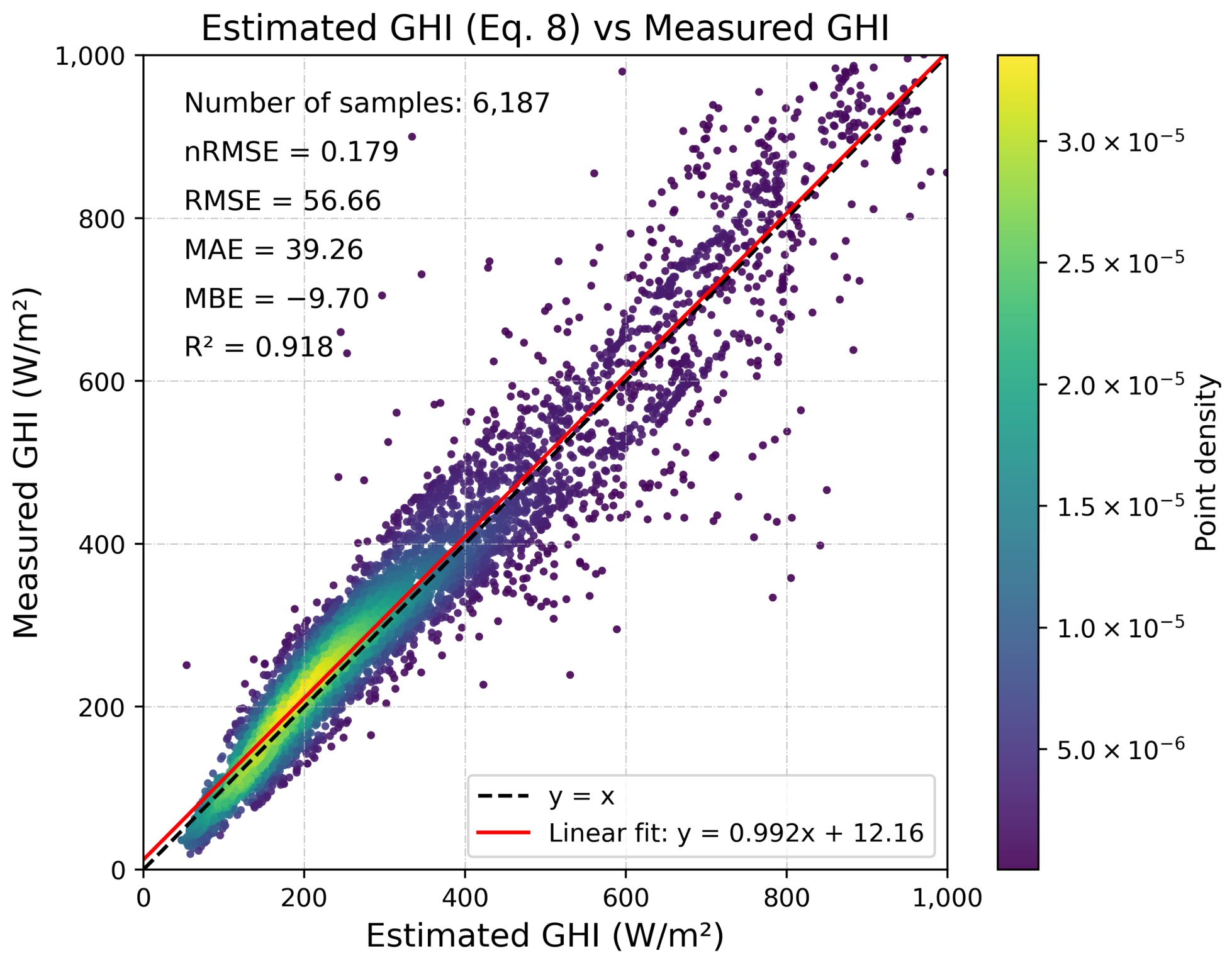
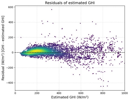
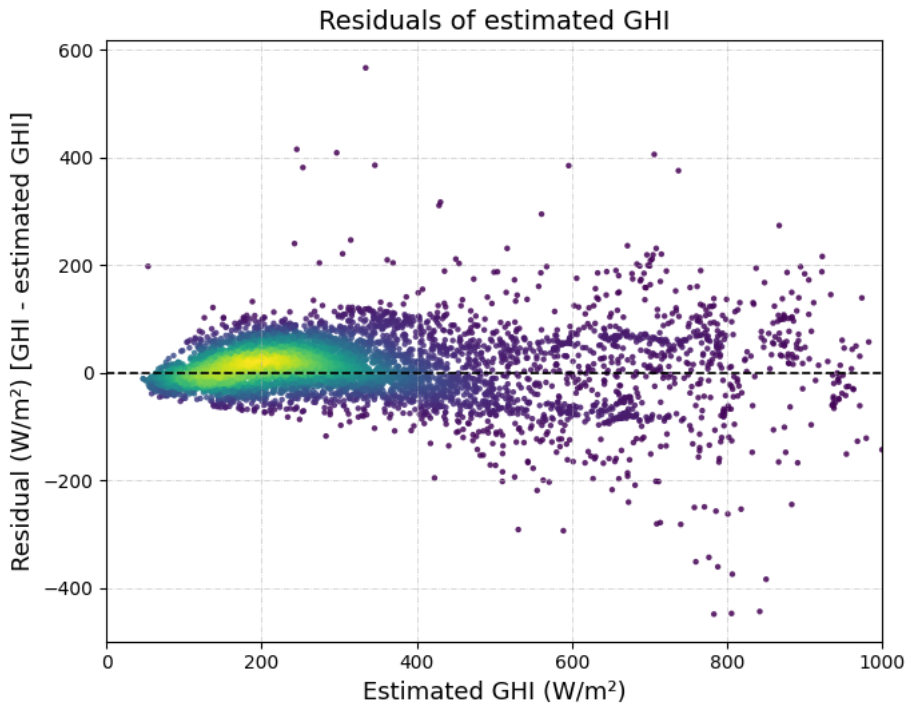
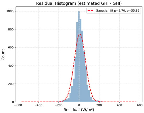
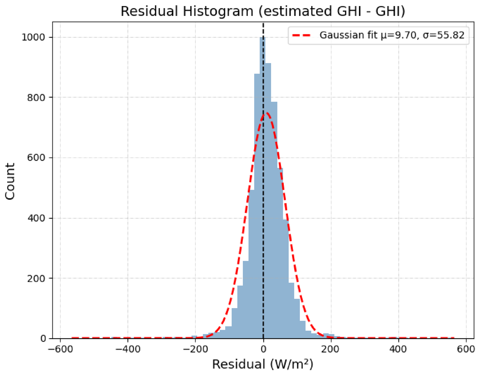

Disclaimer/Publisher’s Note: The statements, opinions and data contained in all publications are solely those of the individual author(s) and contributor(s) and not of MDPI and/or the editor(s). MDPI and/or the editor(s) disclaim responsibility for any injury to people or property resulting from any ideas, methods, instructions or products referred to in the content. |
© 2026 by the authors. Licensee MDPI, Basel, Switzerland. This article is an open access article distributed under the terms and conditions of the Creative Commons Attribution (CC BY) license.