An Integrated Machine Learning and Optimization Framework for Railway Track Quality Assessment: Application to Longitudinal Level

Abstract

Track quality is key to ensuring the safety and comfort of passengers and freight in railway systems. However, continuous monitoring is rarely implemented due to its high cost and technical complexity. This paper introduces a methodological framework based on machine learning and optimization algorithms for developing onboard track quality monitoring systems using inertial measurements. The workflow addresses crucial, often overlooked aspects such as sensor location, integrating them with downstream processes. The methodology was validated through its application to longitudinal level quality estimation. Synthetic acceleration signals were generated using multibody simulations under parameter configurations defined through a Design of Experiments framework. A multi-objective optimization approach was applied to determine the optimal combination of sensors, balancing estimation accuracy and efficiency. Among the evaluated models, XGBoost achieved a root mean square error of 0.175 mm on the test set, requiring only two acceleration signals and vehicle speed. The use of features derived from wavelet spectra instead of traditional statistical descriptors reduced the estimation error by approximately 20%. These results demonstrate the feasibility of constructing low-cost, data-driven monitoring systems for track quality assessment and highlight the benefits of a structured methodology integrating data generation, sensor analysis, and learning algorithms.

1. Introduction

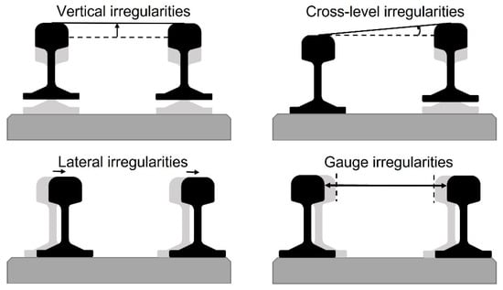
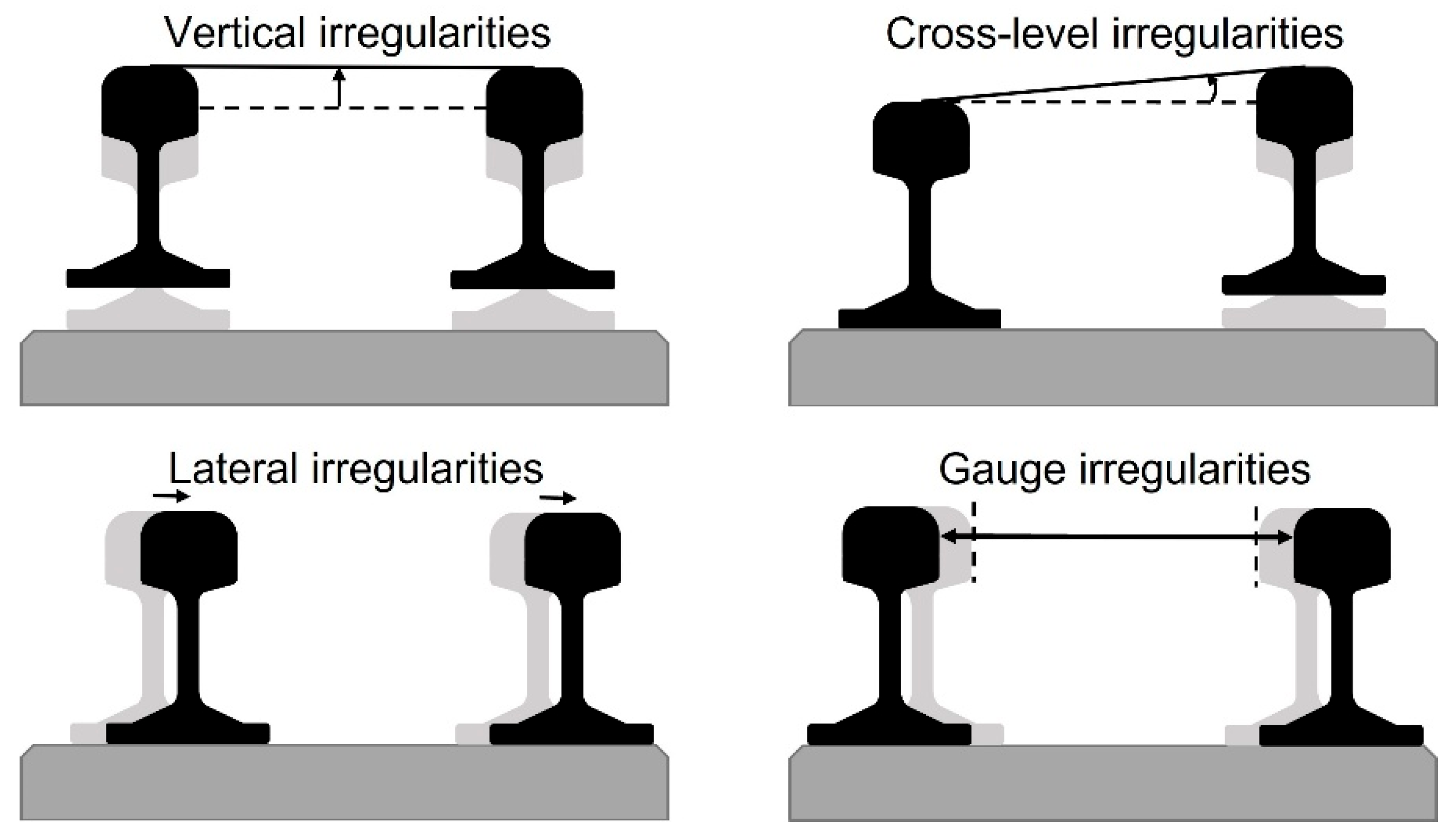
Heterogeneous ballast settlement and stiffness or rail wear and tear, among other factors, lead to deviations in track geometry from its ideal state [1,2]. In particular, variations in track stiffness are closely linked to key deterioration processes such as rail fatigue and the degradation of both superstructure and substructure components throughout the track service life [3]. These effects manifest as geometric irregularities, including deviations in the vertical direction, known as longitudinal level irregularities, or in the transverse direction, referred to as alignment irregularities. Track quality is commonly defined from numerical measurements of these deviations. Specifically, the standard deviation of irregularities is used to establish track quality indices (TQI) in several countries or regions. For example, refer to the European standard EN 13848 [4] or the Chinese TQI [5]. Track irregularities can be described as a combination of the deviations observed in both rails, resulting in four distinct types of track-related irregularities, as illustrated in Figure 1.

Figure 1. Types of track-related irregularities. Arrows and dashed lines represent the displacement of each rail from its ideal position, which is shown in gray.

Track quality directly affects the comfort and safety of passengers and goods transported [6], making the research and maintenance of track conditions a major concern in the railway industry [7,8]. However, traditional track geometry measurement methods are either expensive, such as geometry inspection vehicles, or require modifying the usual traffic, such as manual inspections with a trolley. Additionally, on-board monitoring systems require costly lasers and computational capacity for sophisticated algorithms. These limitations result in infrequent inspections, leading to suboptimal maintenance strategies, unnecessary expenditures, and a lack of accurate knowledge about the actual condition of the railway line. Consequently, the risk of unexpected failures increases, compromising safety and operational efficiency [9,10].

The use of inertial measurements on board in-service vehicles would enable cost-effective, continuous monitoring of railway tracks [11]. Recently, this proposal has received the attention of several researchers. In [12], a Bayesian-optimized improved bidirectional long-short-term memory neural network model is trained to monitor turnouts from car-body accelerations. A Convolutional Neural Network (CNN) is used in [13] to detect damage in rail fasteners. The primary challenge of this kind of system lies in accurately inverting the dynamic interaction between the vehicle and the track. In railway track quality estimation, model-based methodologies rely on mechanistic models of vehicle–track interaction to estimate track irregularities using techniques such as Kalman filtering and model inversion [14]. On the other hand, most recent publications apply data-driven methodologies, supported mainly by emerging Machine Learning (ML) techniques [15]. Features extracted from acceleration signals are applied to train classification models. In [16], support vector machines are trained to identify degraded track sections. Similarly, in [17], random forest and gradient boosting decision trees are applied to subway tracks. Different regression models have been proposed for TQI estimation. Ref. [18] show the correlation between the Root Mean Square (RMS) of longitudinal level and the bogie vertical accelerations in spatial windows and propose a linear regression model. Gaussian regression process, a non-linear model which, in addition, gives a confidence region, is applied in [19]. The reconstruction of track geometry has been addressed by some authors through the application of Deep Learning (DL) techniques, with architectures based on Convolutional Neural Networks (CNN). For instance, ref. [20] combines CNN with an attention mechanism and a Gated Recurrent Unit, and ref. [21] combines CNN with bidirectional long short-term memory, both for the reconstruction of vertical irregularities through the car-body accelerations.

Previous studies have demonstrated the feasibility of estimating track quality from inertial measurements. However, we consider that some key points have not yet received sufficient attention:

• Data origin and diversity: Most authors rely on real data coming from measurements on an in-service train of a certain line to develop their systems. One of the problems with this type of data is its lack of diversity and balance: the data is tied to the line, vehicle, and circulation conditions at the moment of its acquisition. Few works analyze its consequences or attempt to mitigate them. For instance, in [17], the imbalance ratio of the dataset is reduced through a hybrid sampling technique. Other works consider different irregularity levels on a track with curves [22] or different speeds [19,23]. However, in most cases, these variations are explored independently, and the simulation space is not defined through a structured or balanced strategy. Even though multibody system (MBS) simulations allow for the generation of large amounts of data in controlled conditions, from our perspective, their potential remains only partially explored. In particular, combining multibody simulations with a formal experimental design framework could help create balanced datasets, clarify the influence of different factors, and improve reproducibility across studies. We believe that such structured data generation strategies can complement existing approaches and support the development of models with better-controlled generalization properties.
• Sensor location: Track geometry excites different parts of the vehicle in distinct ways, depending on the suspension systems and frequency content involved. Despite this, sensor placement is often chosen for practical convenience or justified only through mechanistic arguments, typically focusing on fixed positions [24]. For instance, as wheel movements are closely related to track geometry, ref. [25] perform double integration of axle box accelerations to obtain wheel displacements. Nevertheless, there are several issues related to the extremely high accelerations in the axle box [26]. In bogie and car-body, accelerations are filtered by the primary and secondary suspension systems, which can be beneficial when working with longer wavelength ranges [27]. The use of multiple sensors distributed across different parts of the vehicle increases the amount of information obtained and enables coverage of a wider wavelength range. Systematic evaluations of alternative layouts are rare. In [28], the authors analyze different sensor layouts based on statistical considerations of acceleration data by applying the ANOVA algorithm to compare six sensor layouts. More recently, ref. [29] includes a sensor layout sensitivity study within their domain adaptation framework, examining how different sensors affect cross-domain defect detection performance. However, both approaches evaluate a limited set of predefined sensor combinations as independent cases. In contrast, we argue that sensor selection must be integrated within the methodological workflow and treated as an optimization problem jointly linked to the final estimation accuracy.

In this article, we propose a methodology that integrates data generation, feature extraction, sensor layout optimization, and machine learning into an end-to-end workflow for track quality estimation. We show how this methodology is applied to the estimation of longitudinal level track quality as a representative use case. Our aim is not to introduce a new high-performance estimator, but to formalize a modular and physically consistent framework that encompasses data acquisition, experimental design, sensor placement, and model training. Section 2 outlines the proposed methodology, while details about its implementation for longitudinal track quality estimation are provided in Section 3. The results obtained are presented in Section 4, and Section 5 discusses the conclusions and outlines directions for future research.

2. Materials and Methods

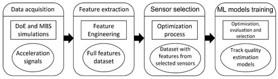
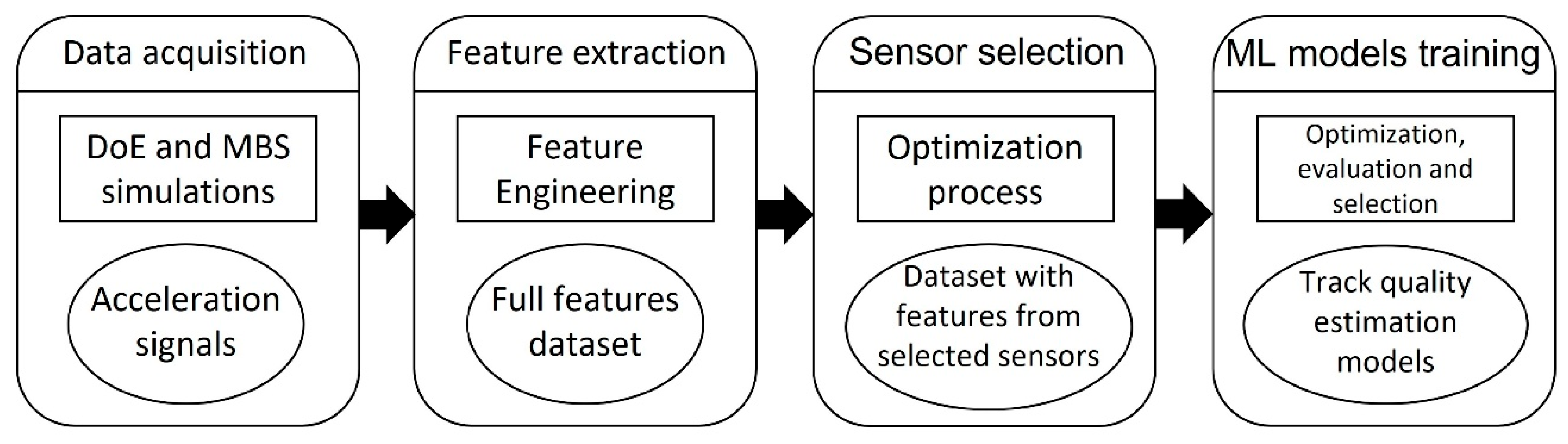
Figure 2 illustrates the steps of our methodology. The setup of the MBS simulations is obtained by a Design of Experiments (DoE) framework, and the generated signals are processed to extract relevant information and features that will form the dataset. The choice of signal processing and feature engineering techniques will depend on the problem specifications and the type of ML algorithm to be used. The next step aims to select an optimal subset of sensors. Again, the optimization techniques and evaluation criteria to apply are linked to the ML algorithms by integrating both aspects of the methodology to ensure coherence and to select the best layout. Finally, the track quality estimation models are trained using the filtered dataset, which contains only the information extracted from the selected sensors. The interpretability of the results will be derived from analyzing the relationship between simulation parameters and the signals, as well as evaluating and inspecting the trained models to understand how they leverage this relationship.

Figure 2. Outline of the proposed methodology.

The remainder of this section provides a step-by-step description of the methodology. To further illustrate the methodology, the particularities of a proposed implementation for the estimation of longitudinal level track quality are given as a use case example. The data employed were generated through simulation of a regional railway vehicle under a wide range of typical operating conditions, track designs, and track irregularity levels, with the aim of obtaining results representative of this type of line while avoiding potential biases associated with more precise use cases. The obtained results are used to illustrate and validate the proposed methodology, as well as to support the interpretation and further understanding of longitudinal track quality estimation based on inertial measurements. These results are not directly applicable to other vehicle models, operating conditions, or objectives. Nevertheless, the proposed methodology is inherently adaptable and is intended to be applicable beyond the specific operating conditions considered here, including different railway systems, vehicle configurations, or track quality assessment objectives.

2.1. Data Acquisition

The success and accuracy of any data-driven methodology are highly dependent on both the quantity and quality of the data used during its implementation. Moreover, the range of applicability of the resultant system is inherently constrained by the variability and conditions represented within the dataset. In practice, acquiring sufficient field measurements is often challenging due to logistical, temporal, or economic limitations. As a result, datasets tend to be unbalanced and biased towards the specific conditions of the vehicle, track, and operational environment. For instance, defective track sections are much less common in an active railway line than healthy sections.

MBS simulations offer a cost-effective alternative to real measurements by generating large amounts of data in customized and controlled configurations. However, the reliability of simulation-based data hinges on the careful definition of the conditions to be modelled. This includes identifying the relevant variables, understanding their real-world variability, assessing the feasibility of accurately modelling them, and evaluating the potential impact of omitting certain factors. A poorly defined simulation space may result in models that fail to generalize or capture critical behaviors.

To address this, it is essential to design simulations that comprehensively span the space of plausible parameter combinations. DoE techniques provide a systematic framework for this purpose, allowing for the efficient exploration of high-dimensional parameter spaces while minimizing redundancy. An effective experimental design is key to reducing the number of simulations required, avoiding imbalances in the training set that can lead to bias and overfitting in ML models, and enhancing the explainability of models by removing any hidden correlation between experiment parameters that could lead to a misinterpretation of the results [30].

The data used in this work were generated through simulations in SIMPACK 2023x.1 software [31] with a 3D vehicle–track model corresponding to a passenger car with two bogies and four wheelsets. The parameters of the vehicle remained constant throughout the simulations. In contrast, the vehicle speed, unbalanced acceleration, cant, friction coefficient, wheel wear, load condition, and track irregularities have been modified from one simulation to the next to analyze the influence of these parameters on the vehicle response and the estimation of track quality.

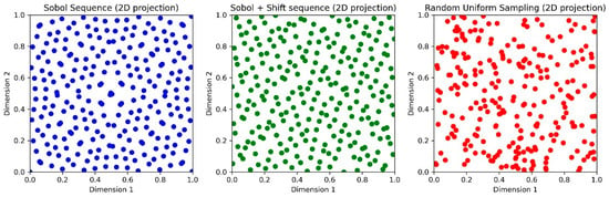
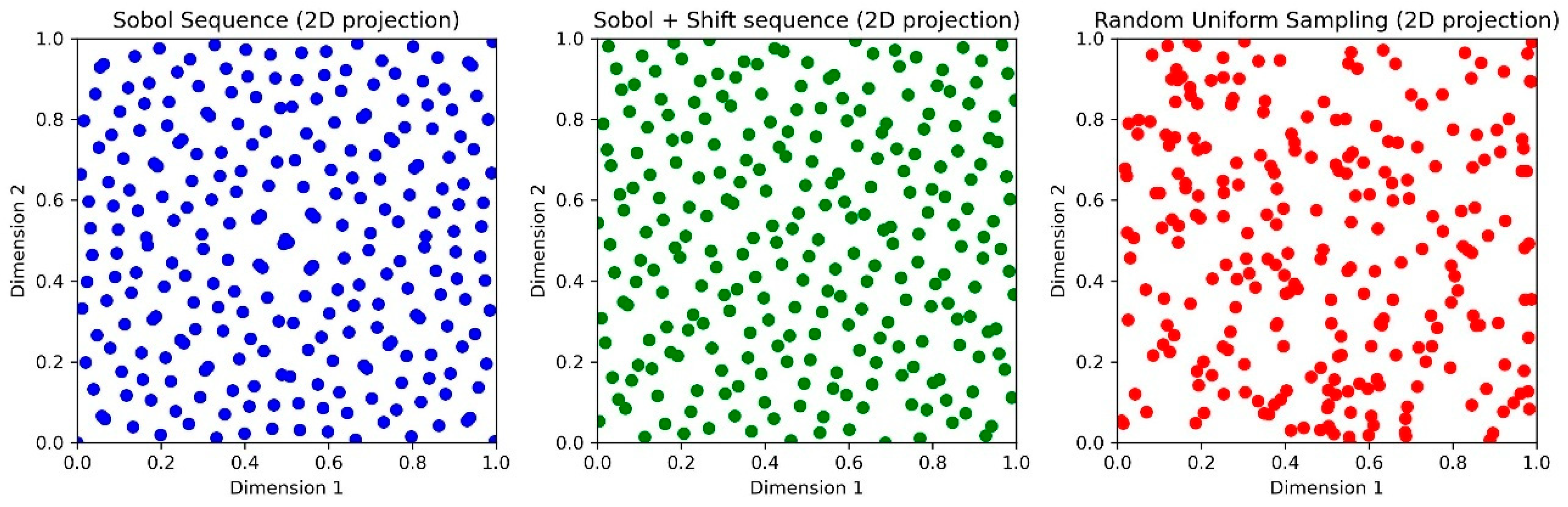
The design of simulations performed is based on the Sobol sequence with a random shift to ensure generating sample points in the design space that meet the properties of distance, uniformity, independence and projection [32]. To illustrate the benefits of this strategy, point distributions obtained with the Sobol sequence, the Sobol sequence with random shift, and a random uniform sampling are compared in a 2D projection in Figure 3. Unlike Sobol-based samplings, the space is not uniformly filled by random sampling, as regions with uneven numbers of points appear. The random shift helps remove any possible correlation between points in the base Sobol sequence.

Figure 3. Samples generated from different methods: Sobol sequence (blue), Sobol sequence with a random shift (green) and random uniform sampling (red).

The Sobol sequence generates points in an s-dimensional unit hypercube. We then obtain the simulation parameters by assigning each dimension to a parameter and scaling it to the desired range. For example, suppose that s is the dimension identified with the vehicle speed, and we want the speed to take values between v₁ and v₂. Then, we get the corresponding speed value by scaling the s dimension of the generated point, $x_s$, to this range: $v=v_1+\left(v_2-v_1\right)x_s$.

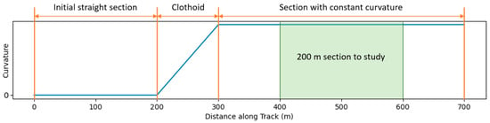
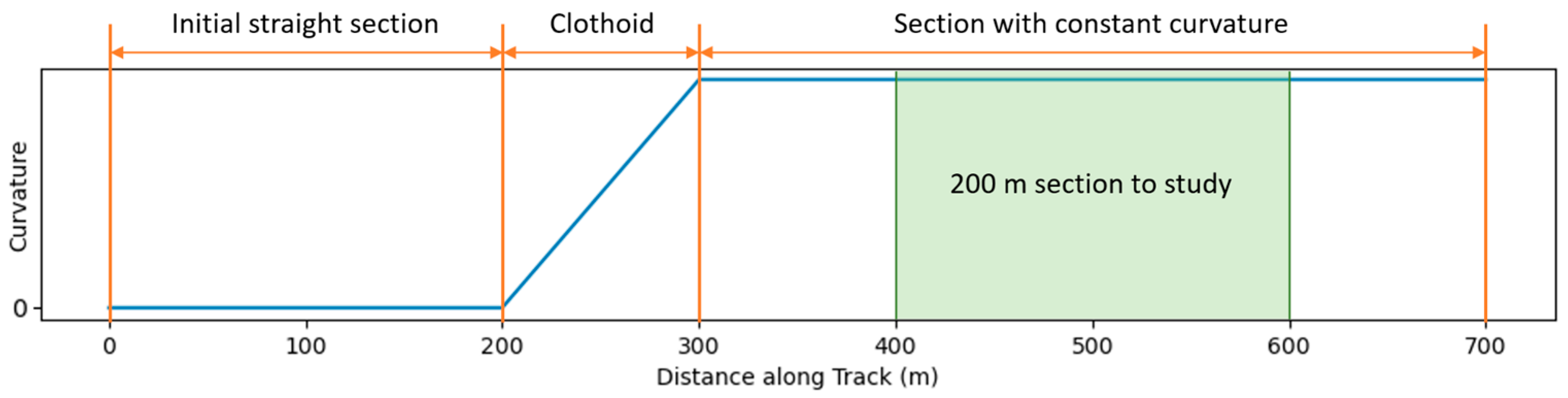
Figure 4 shows the curvature layout used in the simulations. To ensure simulation stability and meet the required cant, running speed, and unbalanced acceleration conditions, each simulation run begins on a straight track section, followed by an entry clothoid. Once the vehicle is fully negotiating the curve, 100 m after the clothoid, the measurements are collected in a 200 m section, as defined by the EN 13848-6 standard [4] for track quality assessment.

Figure 4. Curvature layout of the track used in the simulations. The blue line represents the curvature along the track, the green region denotes the section of constant curvature studied in each simulation, and the orange lines delimit the sections with different curvature regimes.

Irregularities were generated from the standardized power spectral density (PSD) of the four track-related types of irregularities and then scaled to control their standard deviation in realistic operational ranges. The track PSD spectrum is expressed as follows [19,33]:

• Vertical and lateral:

  $$S_{\mathrm{v}/\mathrm{L}}\left(\mathsf{\Omega }\right)=A_{v/l}{\displaystyle \frac{{\mathsf{\Omega }}_c^2}{\left({\mathsf{\Omega }}^2+{\mathsf{\Omega }}_r^2\right)\left({\mathsf{\Omega }}^2+{\mathsf{\Omega }}_c^2\right)}}.$$

  (1)
• Cross-level and gauge:

  $$S_{c/g}\left(\mathsf{\Omega }\right)=A_{c/g}{\displaystyle \frac{{\mathsf{\Omega }}_c^2{\mathsf{\Omega }}^2}{\left({\mathsf{\Omega }}^2+{\mathsf{\Omega }}_r^2\right)\left({\mathsf{\Omega }}^2+{\mathsf{\Omega }}_c^2\right)\left({\mathsf{\Omega }}^2+{\mathsf{\Omega }}_s^2\right)}}.$$

  (2)

  where $\mathsf{\Omega }$ is the spatial angular frequency (rad/m), $A_v, A_l, A_c$ and $A_g$ are scaling factors modified to control the level of the irregularities, ${\mathsf{\Omega }}_c=0.8246$ rad/m, ${\mathsf{\Omega }}_r=0.0206$ rad/m and ${\mathsf{\Omega }}_s=0.438$ rad/m.

Table 1 lists the ranges of simulation parameters. The irregularity level ranges were selected in accordance with the classifications defined in the EN 13848-6 standard [4] for operating speeds below 80 km/h. The remaining simulation parameters reflect typical values observed on conventional railway lines. As irregularities are generated stochastically from their PSD, only the scale, used to match the specified standard deviation values, is completely controlled in each simulation. This provides randomness to the simulations: two simulations with identical parameters can produce different results as long as different seeds are used to generate the irregularities. The standard deviation of the rail-related irregularities is calculated from the generated ones, with identifiers stdLg for longitudinal level irregularities and stdAl for alignment level irregularities. The standardized load conditions for rail vehicles are as follows: AW0 refers to the empty car, AW1 refers to the empty car with seated passengers, and AW2 refers to the empty car with seated passengers and 2 standing passengers per square meter. The wheel profile levels employed are a new profile, and the profile worn after almost 50,000 km and after almost 100,000 km. The selected parameter ranges are representative of standard regional railway operation. However, the methodology can be reapplied using tailored data to get results applicable to other types of railway lines, to achieve more dedicated and optimal performance in specific situations, or to address extreme conditions outside the considered ranges.

Table 1. Short identifiers and value ranges of simulation parameters.

Parameter	Identifier	Type	Values/Ranges
Std. vertical irr. (mm)	stdV	Numerical	0–4
Std. lateral irr. (mm)	stdL	Numerical	0–3.1
Std. cross-level irr. (mm)	stdR	Numerical	0–4
Std. gauge irr. (mm)	stdG	Numerical	0–3.1
Load condition	M	Categorical	AW0, AW1, AW2
Speed (km/h)	vel	Numerical	25–80
Friction coefficient	Friction	Numerical	0.1–0.5
Unbalanced acceleration (m/s2)	uacc	Numerical	−0.4–0.4
Cant (m)	cant	Numerical	0–0.15
Wheels profile	Wheels	Categorical	3 wear levels

2.2. Feature Extraction

Measured acceleration signals are highly dimensional data. This characteristic poses a challenge for ML models, hindering the uncovering of the hidden patterns and relationships useful for track quality estimation among the large number of data points. Transforming the acceleration signal into features can improve the accuracy of ML models while also reducing their size and complexity and enhancing their interpretability.

In several previous works, statistical features are calculated from signals to train ML models or use them as TQI. In particular, the Root Mean Square (RMS) of accelerations is broadly employed in the literature as it shows a significant correlation with the standard deviation of irregularities, especially in the vertical case. Additional statistical features usually extracted are peak-to-peak values, or entropy and crest factor, among others [22,34,35,36].

Information in the frequency domain is accessible via the Fourier transform; however, temporal context is lost. The wavelet transform provides a time-frequency representation by breaking down the signal into scaled and translated versions of a mother wavelet [37]. This approach facilitates multiresolution analysis of the spectrum and exhibits superior flexibility when compared to the Short-Time Fourier Transform. Consequently, it stands as a powerful tool for the location and detection of changes within non-stationary signals [38] and modal identification [39].

For the estimation of longitudinal level track quality, two different feature extraction approaches have been compared. On the one hand, several statistical measures of the acceleration signals were calculated: RMS, peak-to-peak factor (p2p), skewness, kurtosis, dominant frequency, and spectral entropy. On the other hand, the wavelet spectra of accelerations were generated.

To reduce the dimensionality of the wavelet spectra, principal component analysis (PCA) was applied [40]. With just a few components, a large portion of the useful information contained in the spectra can be extracted. By performing various tests, we have observed that applying PCA to the wavelet spectra is more effective than applying it directly to the signal time series. This is likely because the spectral representation captures the essential frequency components of the signal, reducing noise and irrelevant variations that are present in the time domain. The first 10 principal components of each spectrum were used.

Statistical features and wavelets+PCA approaches were applied independently, along with a third approach that combined the two sets of features, to analyze and compare their effectiveness as predictors for estimating longitudinal track quality. The extracted features and their identifier are listed in Table 2.

Table 2. Extracted features identifiers.

Feature	Identifier
Root mean square	rms_X
Peak-to-peak acceleration	p2p_X
Skewness	skewness_X
Kurtosis	kurtosis_X
Dominant frequency	dominant_freq_X
Spectral entropy	spectral_entropy_X
N principal component	X_cN

2.3. Sensor Location

Simulations enable the measurement of accelerations at multiple points distributed throughout the vehicle. However, in real life, we are interested in using as few sensors as possible to facilitate installation and maintenance and simplify data processing. Furthermore, correlated or redundant data can negatively affect the performance of ML models.

In response, the following phase of the methodology focuses on determining the most effective layout of sensors. Leveraging the capacity to generate data from multiple locations on the vehicle, we propose conducting a systematic search for sensor combinations that identify those offering the best trade-off between estimation accuracy and the number of sensors required.

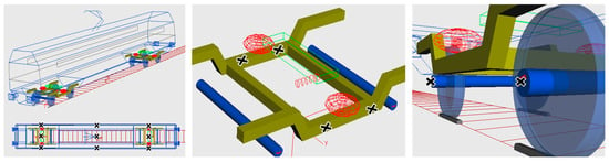
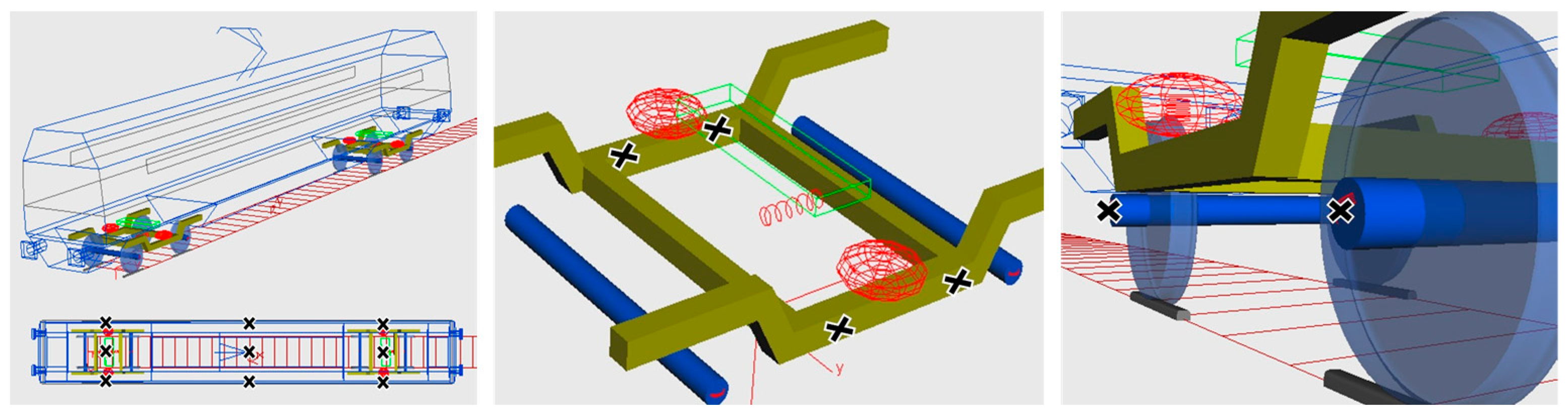
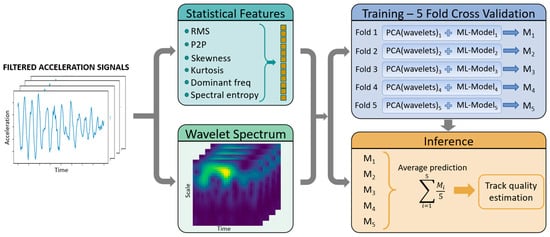
The locations of the sensors placed in the simulated car are shown in Figure 5. Specific locations are described in Table A1 of the Appendix A. The sensors used are understood as uniaxial accelerometers. This means that at each of the 25 specified positions, three distinct sensors could be located, each corresponding to a different axis (longitudinal, vertical, and lateral), for a total of 75 potential acceleration signals.

Figure 5. Placement of the acceleration sensors (represented by the symbol “X”) on the simulated vehicle: on the car-body (left), on the bogie (center), and on axle boxes (right). The colors and lines shown in the SIMPACK screenshots are used to visually distinguish different vehicle components and reference geometries and do not encode additional quantitative information.

Due to the geometry of the system, fourteen of these signals were found to be redundant and were consequently removed: lateral accelerations on each cross-section of the car-body (6 removed signals); lateral accelerations on each axle box of a wheel axis (4 signals); and the longitudinal acceleration on each side of the bogie frame (4 signals). The final analysis was therefore performed on 61 unique acceleration signals.

In this work, the fast training speed of compact models has been leveraged to design a sensor selection strategy that explicitly accounts for the predictive capability of the features extracted from each sensor signal, rather than relying on prior statistical balances decoupled from the final prediction task. The objectives are to reduce both the number of required sensors and the error of estimation. These objectives are not expected to be jointly optimized: while the minimum possible number of sensors is one, it is unlikely that the lowest prediction error can be achieved using a single sensor. Multi-objective optimization (MO) is applied to this kind of problem to get the best trade-off solutions, called the Pareto optimal solutions or Pareto front [41]. The NSGA-II [42] is one of the most popular MO algorithms. It employs non-dominated sorting, crowding distance, and elitism to approximate the Pareto front efficiently, balancing convergence and diversity.

The search space consists of all possible sensor combinations. In addition to these, other parameters are also included in the search space: vehicle speed, load condition, unbalanced acceleration, cant, wheels and friction coefficient. In this context, we include these parameters when referring to “sensors” to avoid naming both explicitly. The two objective functions to minimize are the number of selected sensors and the error that a baseline ML model yields on a test dataset. The model is trained with data coming from chosen sensors: extracted features from the corresponding acceleration signals (combining both statistical measures and the principal components of wavelets) and the value of parameters, if any. Since it showed both training speed and strong performance, as shown in the results section, the XGBoost was used as the benchmark ML model during the algorithm iterations [43]. Although the Pareto front sensor combinations may vary slightly depending on the chosen model, we have not observed substantial changes between the models capable of capturing non-linear relationships. The models are trained with 5-fold cross-validation. The error metric considered by the algorithm is calculated as the mean of the Root Mean Squared Error (RMSE) values across the validation folds.

The training workflow followed for this step is identical to the one described in detail in the following section, with the exception of hyperparameter optimization. Incorporating a dedicated hyperparameter tuning process at this stage would have significantly increased the dimensionality of the search space and rendered the evaluation of every sensor combination computationally impractical. Consequently, while the exact Pareto-front solutions may depend on the choice of hyperparameters and the learning model, the overall trends and conclusions regarding the relative performance of the sensor combinations were found to be robust across different non-linear models and reasonable hyperparameter settings.

The primary objective of this step of the methodology is therefore to identify a reasonably informative sensor combination and to assess how estimation performance varies as a function of the selected sensor set, rather than to determine a strictly optimal configuration. We acknowledge that the gap between the models and data used in this exploratory phase and those ultimately deployed for real-world inference may lead to a suboptimal sensor choice in practice. Nonetheless, this analysis provides a consistent and computationally tractable basis for comparing sensor configurations and understanding their relative impact on estimation capability.

2.4. ML Models Training

Once an optimal sensor layout is selected, the final step of our methodology involves using the acceleration signals measured by the sensors to train ML models. These trained models are then employed to estimate the target track quality indicator.

The ML models must be carefully chosen according to the objective pursued: classification or regression of a TQI or estimation and reconstruction of track geometry. Another important aspect to consider is the trade-off between accuracy, robustness, generalization power, and computational efficiency and cost. Model interpretability might also be a key factor in some cases. Moreover, the amount of data available and its characteristics can limit the capabilities of the models.

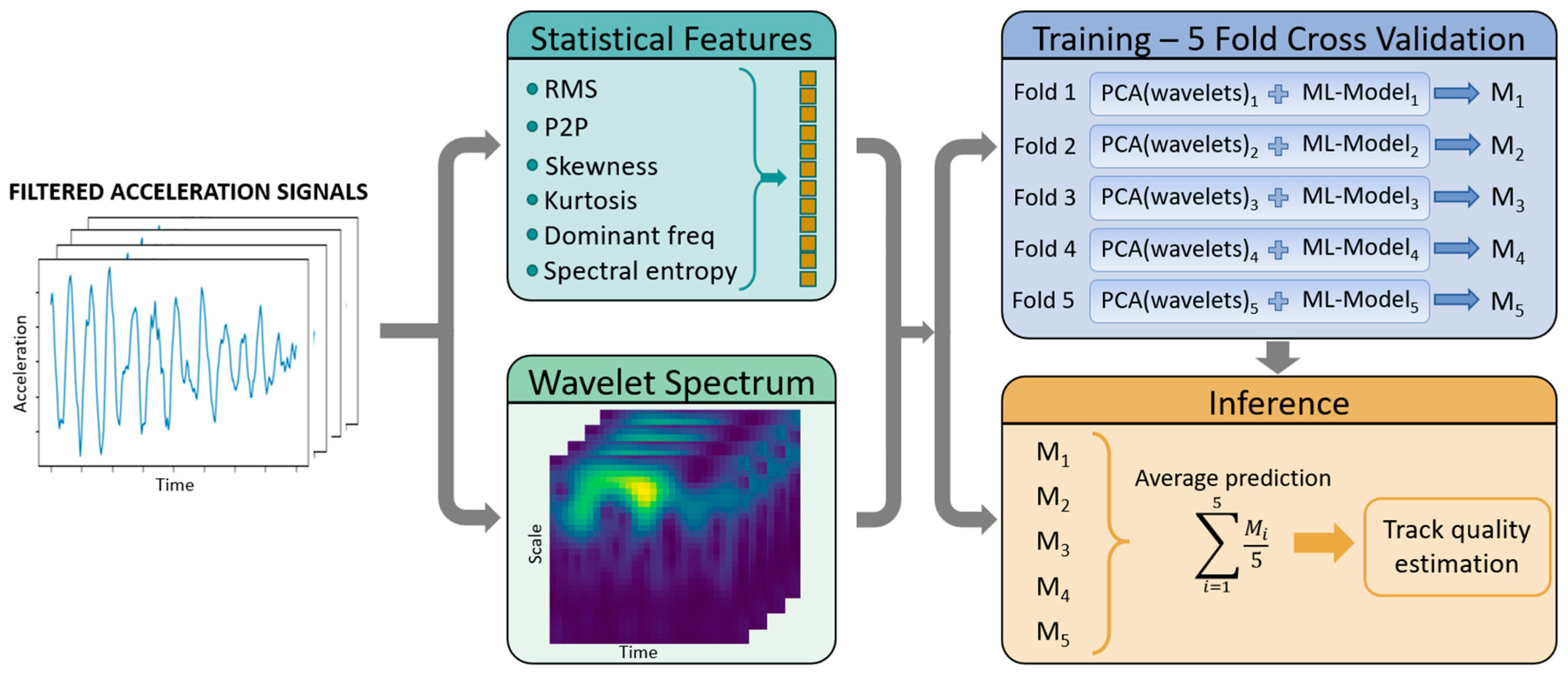
Given the synthetic nature of the dataset, our primary objective is to validate the consistency and logic of the problem formulation rather than to maximize predictive performance metrics through high-capacity models. Consequently, we employ traditional ML algorithms instead of complex DL networks. This choice avoids the risk of the model overfitting to the generative artifacts of the synthetic data and ensures that the observed results are attributable to the methodology itself rather than the architectural complexity of the learner. Since we are working with tabular data, we selected several regression models that are particularly effective for this data structure. Specifically, we employed Linear Regression (LR), Decision Tree (DT), Random Forest (RF), Gradient Boosting Machine (GBM), XGBoost (XGB), and MultiLayer Perceptron (MLP) [44], and the standard deviation of longitudinal level irregularities in a 200 m section as TQI. RMSE served as the primary metric for both model training and performance comparison. To improve the capability of these models, hyperparameter tuning was carried out using the Tree-structured Parzen Estimator (TPE) algorithm [45], which prioritizes promising regions of the search space based on prior evaluations. The dataset was split into 20% exclusively for testing and 80% for training the models via 5-fold cross-validation. Figure 6 shows the approach we have followed. First, statistical features and wavelet spectra are calculated from the filtered acceleration signals. Then, ML models are trained along with the PCA of the wavelets corresponding to the training fold. Finally, inference is performed on the test set with the trained models.

Figure 6. Flowchart of the followed approach for training track quality estimation models. In the wavelet spectrum, brighter colors represent regions of higher energy.

Finally, a variable influence analysis was conducted to enhance model interpretability, providing insights into feature importance.

3. Results

In this section, the results of the proposed methodology applied to the estimation of longitudinal track irregularities are presented.

3.1. Analysis of Simulation Results

To analyze the influence of simulation parameters on vehicle accelerations, it is essential to consider possible non-linearities and interactions between features. Surrogate XGB models have been trained using simulation parameters as inputs and the RMS of each acceleration sensor as output. Each trained model serves as an approximation of the simulation that uses simulation parameters to estimate the RMS value of an acceleration signal. The surrogate models cannot fully replicate the behavior of the mechanistic models, as they lack detailed information about the shape of the irregularities and rely solely on their standard deviation, thus introducing additional noise.

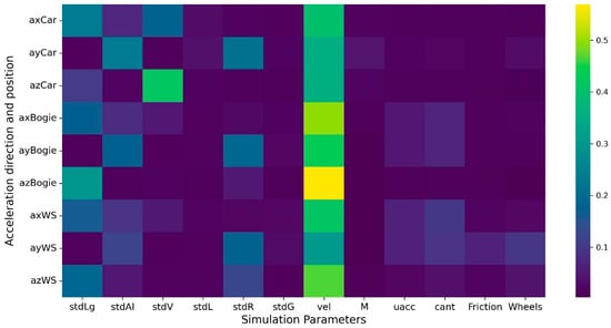
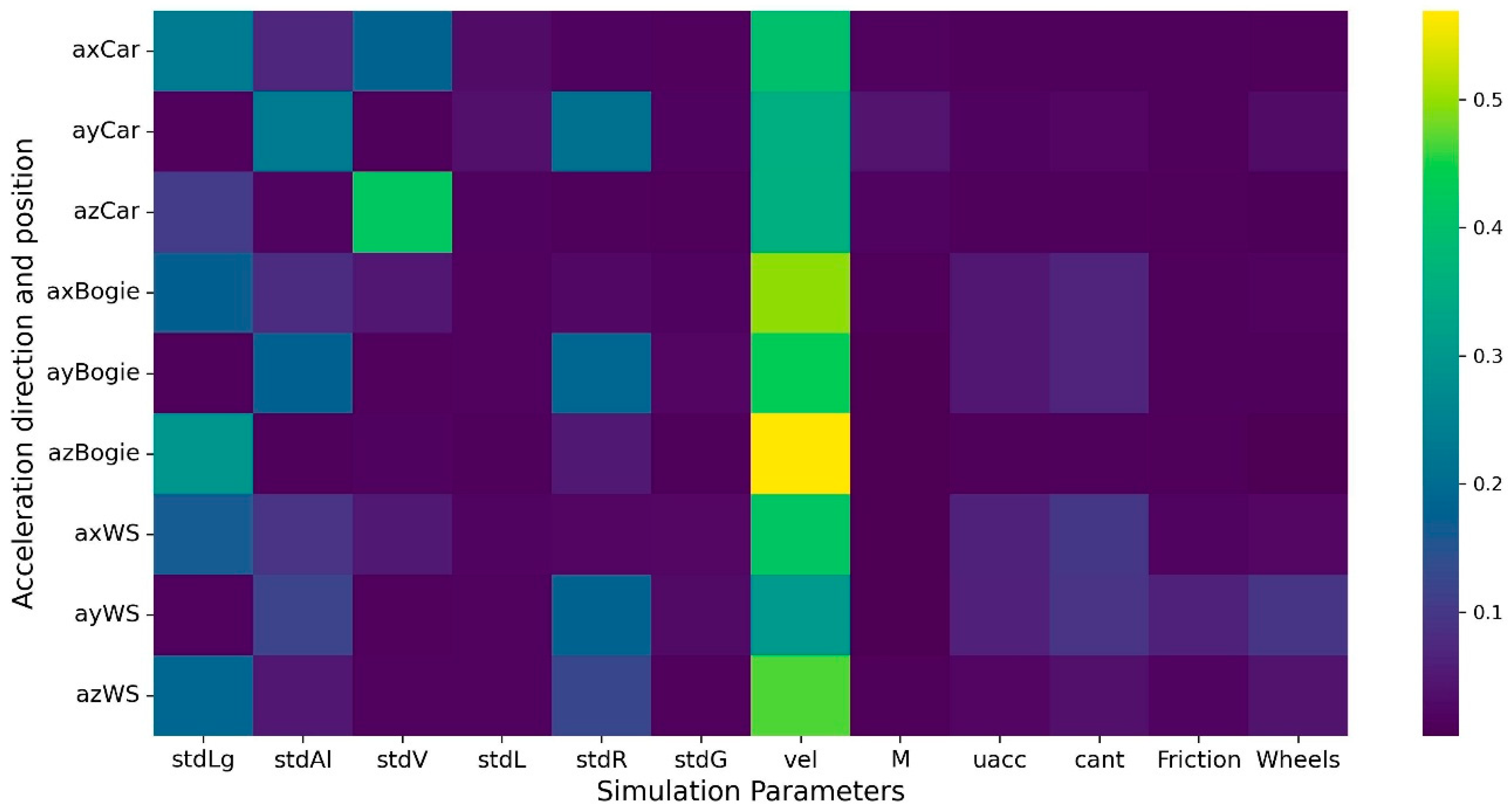
Shapley values, originating from cooperative game theory, provide a robust method to interpret the contributions of individual features to the predictions made by a machine learning model [46]. In our case, Shapley values measure the influence of each simulation parameter on the acceleration estimations. Figure 7 illustrates the averaged and scaled Shapley values. Vehicle speed makes an important contribution to all the surrogate models, which means that speed influences the dynamics of the vehicle elements. Irregularities heterogeneously contribute to the accelerations. In the case of longitudinal and vertical irregularities, large Shapley values were obtained for the estimation of the vertical and longitudinal acceleration of the car-body and bogie, in the same line as the observations from the correlation analysis. Therefore, these accelerations can be expected to be important in the estimation of longitudinal irregularities. Other simulation parameters got small Shapley values, meaning that their influence on the measured accelerations is minor.

Figure 7. Scaled Shapley values of simulation parameters in the surrogate models for RMS estimation of accelerations at the different parts of the vehicle.

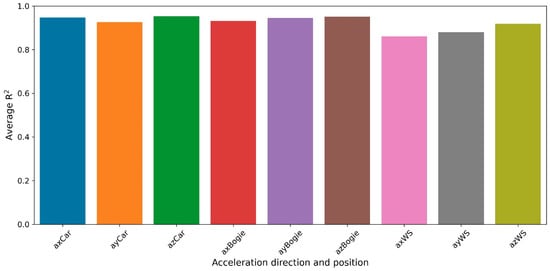
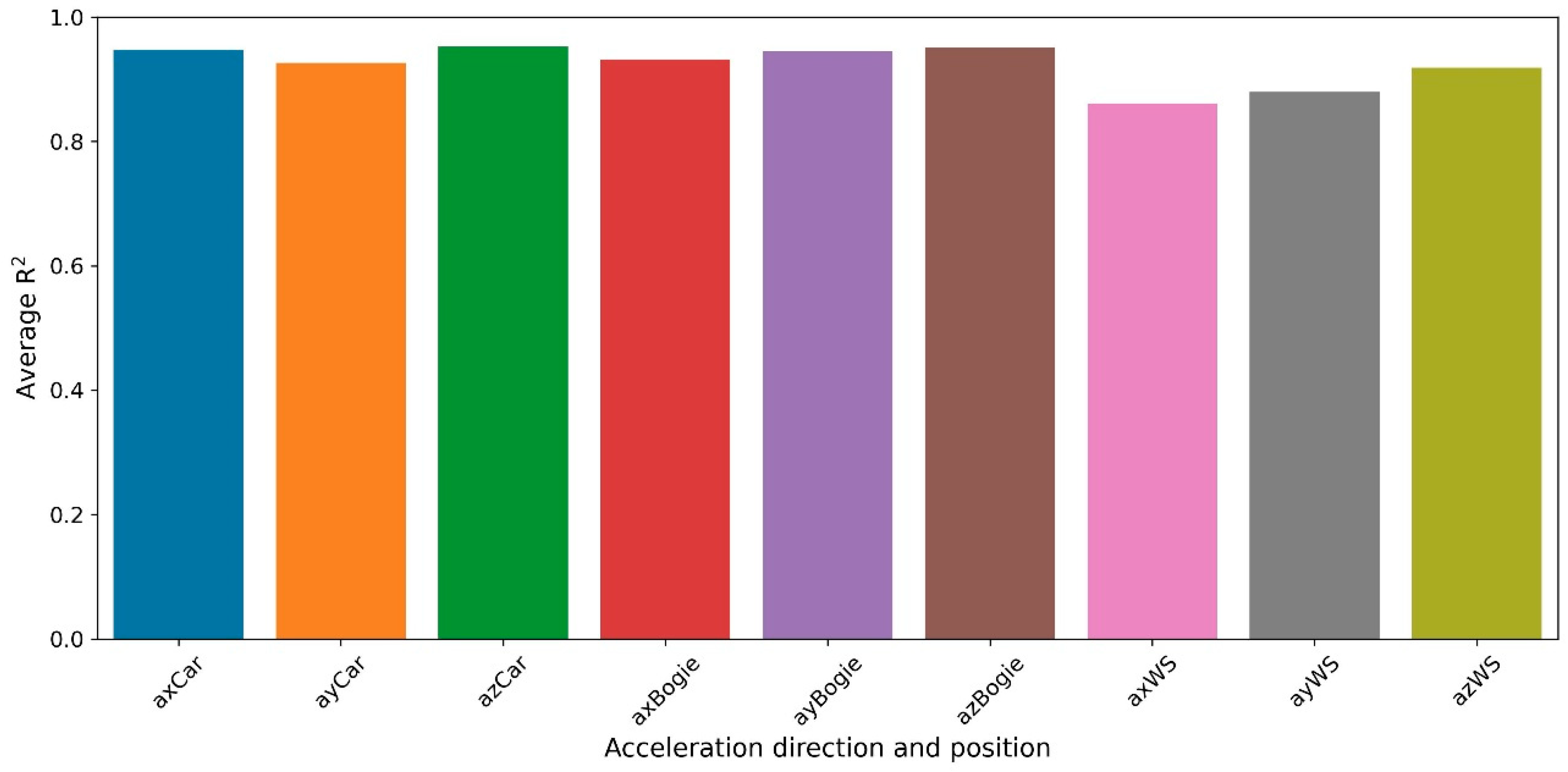
As Shapley values describe the contribution of parameters in the surrogate models, the exposed values and insights are only valid if the models are accurate enough. The coefficient of determination, or R² score, is a metric that represents the proportion of the variation that can be predicted. In our case, all models had an averaged R² greater than 0.86, which indicates that the models explain more than 86% of the variability in the output data. Therefore, while the precise contributions of the parameters may have slight variations, the Shapley values are sufficiently representative for the qualitative analysis presented.

Figure 8 shows the R² score obtained in the estimation of each group of accelerations. The accuracy of the surrogate model can be interpreted as a measure of the complexity of the accelerations in response to the simulation parameters and the influence of the underlying irregularities. The highest accuracies were obtained in the estimation of accelerations on the car-body and bogie. This suggests a reduced sensitivity of these vehicle elements to the precise shape of the irregularities, likely due to the damping and filtering effects introduced by the suspension system. Rather than being a disadvantage, this reduced sensitivity can actually facilitate the estimation of aggregate TQIs by minimizing noise and artifacts.

Figure 8. Average R2 score of the surrogate models. The bar colors are used solely for visualization purposes to distinguish between sensors and do not encode additional information.

3.2. Results of Sensor Location Strategy

The potential number of sensors available is substantial, comprising 61 acceleration signals and 6 simulation parameters. However, we anticipated that optimal sensor layouts would have a significantly reduced number of sensors. To enhance the convergence of the MO algorithm towards sparser solutions, instead of representing each sensor with a binary choice (0 = not selected, 1 = selected), five possible integer values for each sensor, ranging from 0 to 4, were established. A sensor was only considered ‘selected’ if its assigned value in a given trial was 4. This encoding strategy significantly influenced the initial populations; on average, the number of randomly selected sensors in the initial population was reduced from over 30 to approximately 13. While still relatively high, this figure is considerably closer to the expected optimal sparsity.

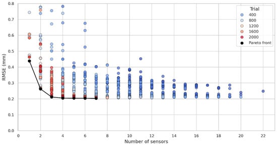
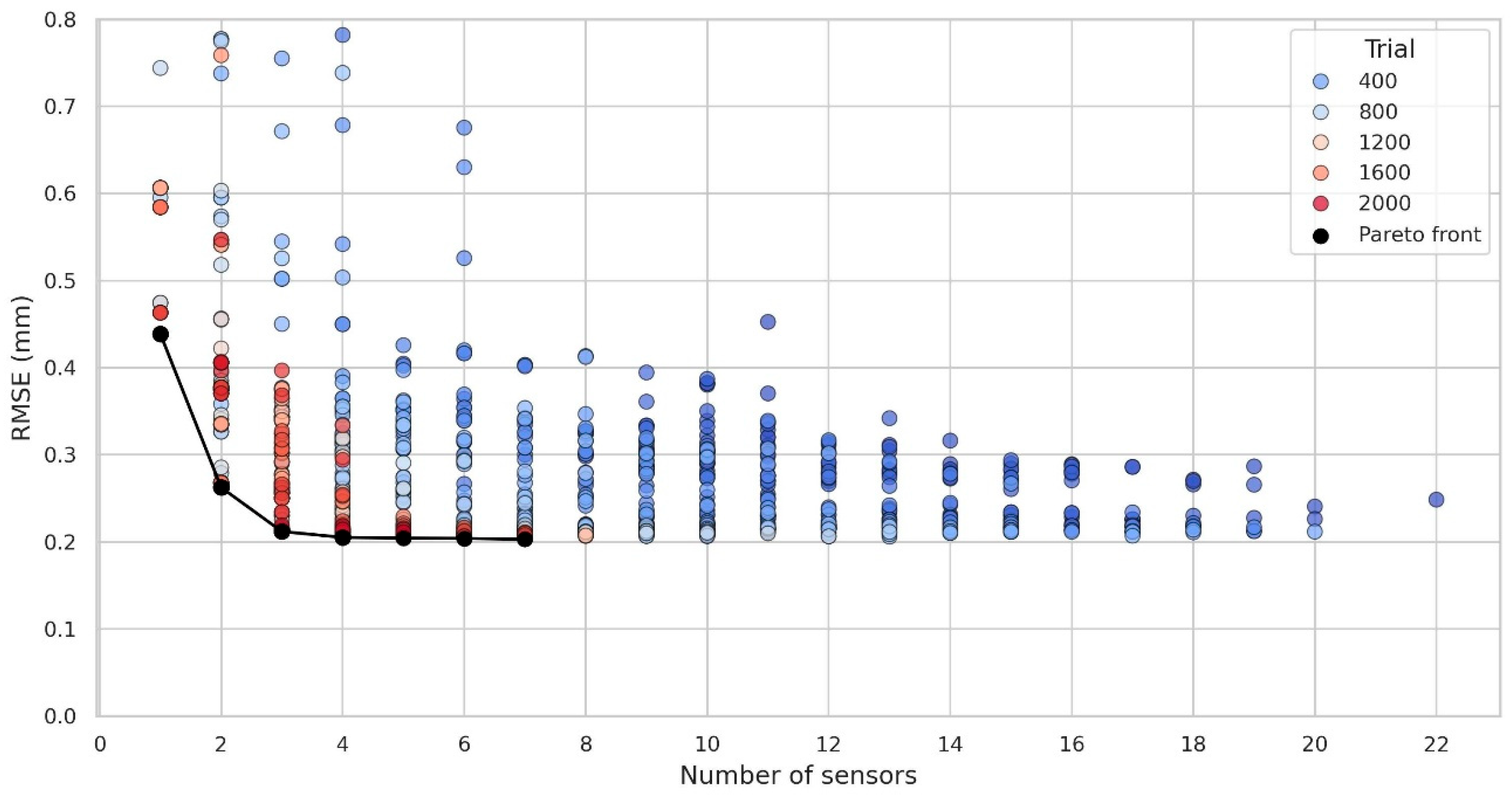
The Optuna 4.2.1 framework was used to implement the sensor selection strategy in Python 3.11.11 [47]. The MO algorithm was executed for 2000 trials, with each generation comprising a population of 50 trials. As depicted in Figure 9, the number of sensors was progressively reduced through successive algorithm iterations, and superior combinations were identified until convergence on the Pareto front was achieved. The specific sensor combinations forming the Pareto front are detailed in Table 3.

Figure 9. Error and number of sensors of the sensor combinations tried by the NSGA-II algorithm. The points that form the Pareto front are highlighted.

Table 3. Sensor combinations of the Pareto front.

Sensors	Number of Sensors	RMSE (mm)
azCar_CC	1	0.439
azBogie_F_RB, vel	2	0.262
axCar_RC, azBogie_F_LB, vel	3	0.212
axCar_RC, azBogie_F_RF, azBogie_F_LB, vel	4	0.205
azWS4_L, axCar_RC, azBogie_F_RF, azBogie_F_LB, vel	5	0.204
azWS4_L, axCar_RC, azBogie_F_LF, azBogie_F_RB, ayBogie_F_LF, vel	6	0.204
azWS4_L, axCar_RC, azBogie_F_LF, azBogie_F_RB, axBogie_R_LB, ayBogie_F_LF, vel	7	0.203

The Pareto front revealed that vertical and longitudinal accelerations of the car-body and bogie, along with vehicle speed, are the most relevant sensors. This follows the observations of the previous analysis. Furthermore, no significant improvement in performance was observed when including more than four sensors, which represents a practical benefit. While the Pareto front solutions represent the best-performing sensor layouts, numerous other combinations yield comparable results (other trials in the graph that do not belong to the Pareto front). Therefore, when transferring these findings to a real vehicle, practical considerations such as installation feasibility, wiring constraints, and long-term maintenance effort should also guide the final choice of sensor configuration.

3.3. Track Quality Estimation Results

Several ML models were trained to estimate longitudinal irregularities from the features extracted from the axCar_RC and azBogie_F_LB sensors and the vehicle speed. The Optuna framework was again utilized for model hyperparameter optimization, and models were trained in Python using Pytorch 2.5.1 for the MLP [48] and Scikit-learn for the remaining models [49]. Best hyperparameters found are collected in Table A2, Table A3, Table A4, Table A5 and Table A6 of the Appendix A.

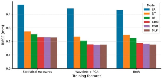
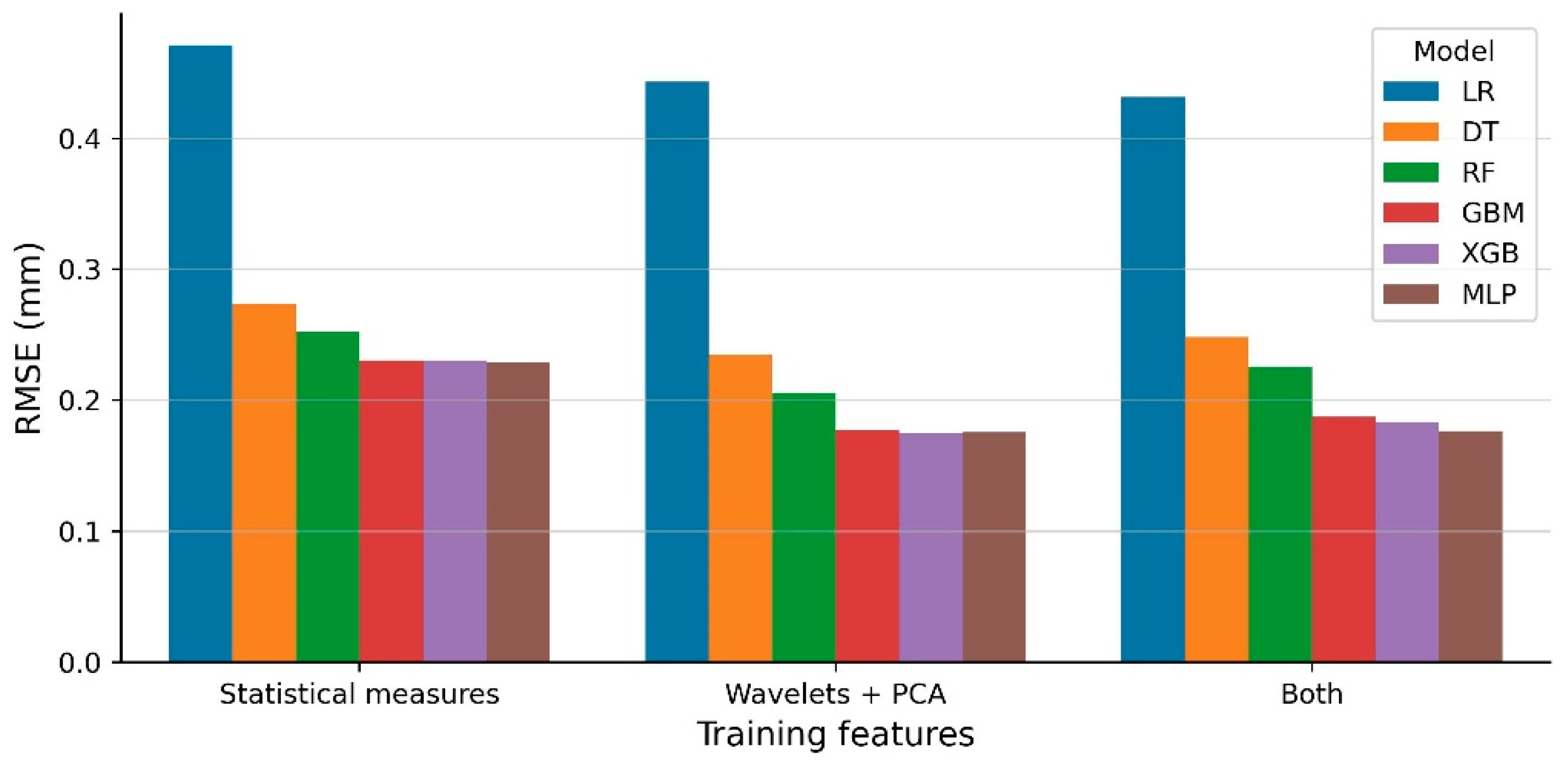
To comprehensively evaluate the improvement offered by the introduction of PCA applied to wavelet spectrum, we trained the ML models using two distinct feature sets: only the statistical measures and only the first 10 principal components derived from the wavelet decomposition. For a fair and rigorous comparison, a specific hyperparameter search was executed for each unique combination of model and training data.

Figure 10 illustrates the error achieved on the test dataset for each trained model under these conditions. The principal components of the signal wavelets yielded superior results compared to the statistical measures. This behavior is consistent with the ability of wavelet-based representations to capture nonstationary and multi-scale signal characteristics, while the subsequent PCA step emphasizes dominant patterns and attenuates noise-dominated components. This indicates that the relative advantage over traditional statistical features may remain robust in the presence of unmodeled disturbances, as typically encountered in real-world data. In addition, combining both feature sets led to a slight decrease in performance. This outcome suggests that the statistical features do not contribute meaningful additional information beyond what is already captured by the wavelet components. Moreover, the inclusion of redundant or weakly informative features may introduce noise and increase model complexity, potentially hindering generalization and reducing predictive accuracy.

Figure 10. Models error achieved with different sets of features.

Table 4 shows the RMSE values obtained on the test dataset by the models trained using the principal components of the wavelets, along with the training and inference times for each model. Models were trained on an Intel^® Xeon^® Gold 5420+ CPU, limited to 8 threads, with sufficient memory given the size of the models and dataset. Among the evaluated models, GBM, XGB, and MLP models clearly outperform others in terms of accuracy. Since the RMSE values are similar across these three models, training times and computational efficiency become important considerations. In this context, XGB demonstrates the fastest training time and was therefore adopted as the benchmark model for subsequent analyses involving simulation parameters and sensor selection.

Table 4. Error on the test dataset obtained with each ML model and their average training and inference times.

Model	RMSE (mm)	Training Time (s)	Inference Time (ms)
Linear Regression	0.443	0.01	0.44
Decision Tree	0.235	0.15	0.51
Random Forest	0.206	4.49	114
GBM	0.177	30.48	0.68
XGB	0.175	1.43	2.0
MLP	0.176	17.13	0.04

In practical applications, inference latency is also a relevant consideration, particularly when computational resources are limited. The differences observed across models, most notably for Random Forest and the MLP, are largely attributable to the specific implementation and optimization strategies of each approach rather than to fundamental differences in model complexity, especially in the regime of single-sample inference, where fixed computational overhead plays a significant role. Ultimately, the methodology remains flexible, as computationally efficient models such as XGBoost can be used during the sensor selection and design stages, while the final inference in real-world deployments may rely on a different model depending on latency and infrastructure constraints.

4. Discussion

While the quantitative results demonstrate that the proposed sensor selection strategy enhances estimation capabilities, a qualitative interpretation offers valuable insights into what each sensor measures and how they complement each other.

In the single-sensor configuration, the optimal signal is the vertical acceleration at the center of the car-body. The car-body is less sensitive to the vehicle speed than other components due to the secondary suspension system. Furthermore, in the center, the vertical movement is less affected by pitch or roll movements.

The two-sensor solution incorporates the vertical acceleration in the front bogie and the vehicle speed, considerably improving the estimation capabilities. By explicitly including vehicle speed as a predictor, the dependency of bogie accelerations on speed is no longer an obstacle. Furthermore, it benefits from a broader frequency response range than the car-body while filtering the strong impacts at the wheels via the primary suspension [33], and avoids the bounce and pitch geometric filters present in the car-body in the studied range of wavelengths [50].

Vertical irregularities not only induce vertical accelerations but also pitch motions. The third sensor selected is the longitudinal acceleration at the rear of the car-body, which accounts for pitch dynamics, providing further insights about the vertical track profile.

Finally, in the four-sensor configuration, vertical accelerations at both the left and right sides of the bogie are selected, offering decoupled information on the two rails. This configuration represents the maximum extractable information considering the capabilities of our models. With more complex regression models, finer details of the vehicle–track interaction could be resolved, potentially leading to slight variations in the optimal sensor set.

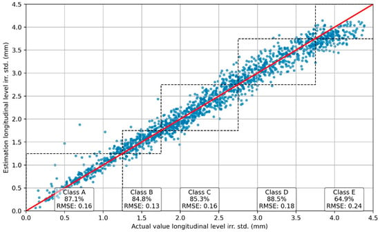
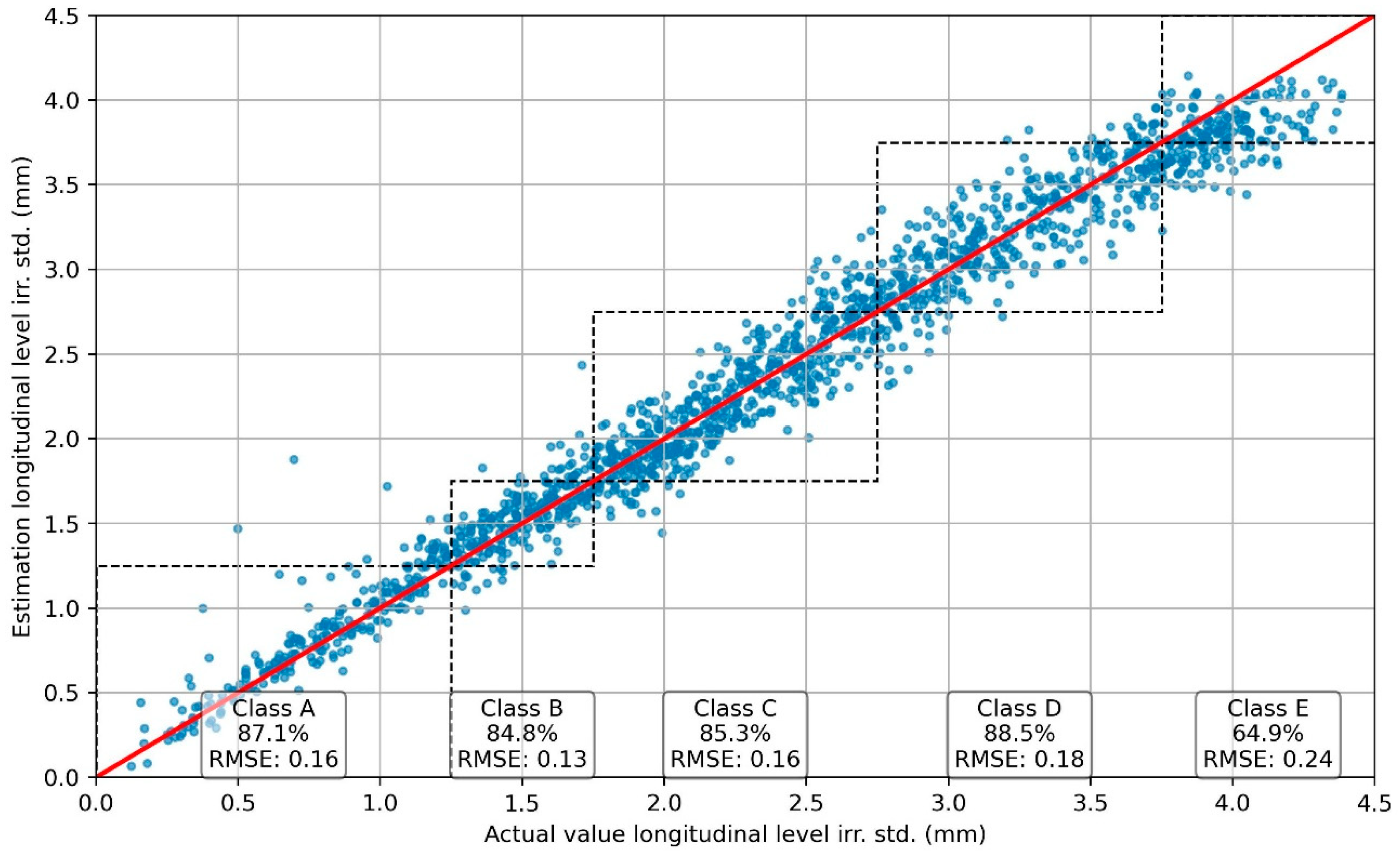
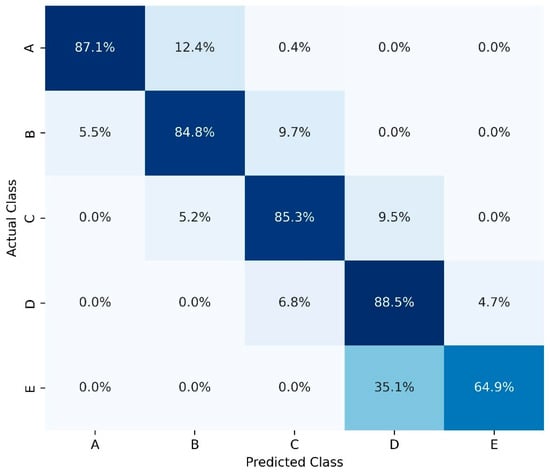
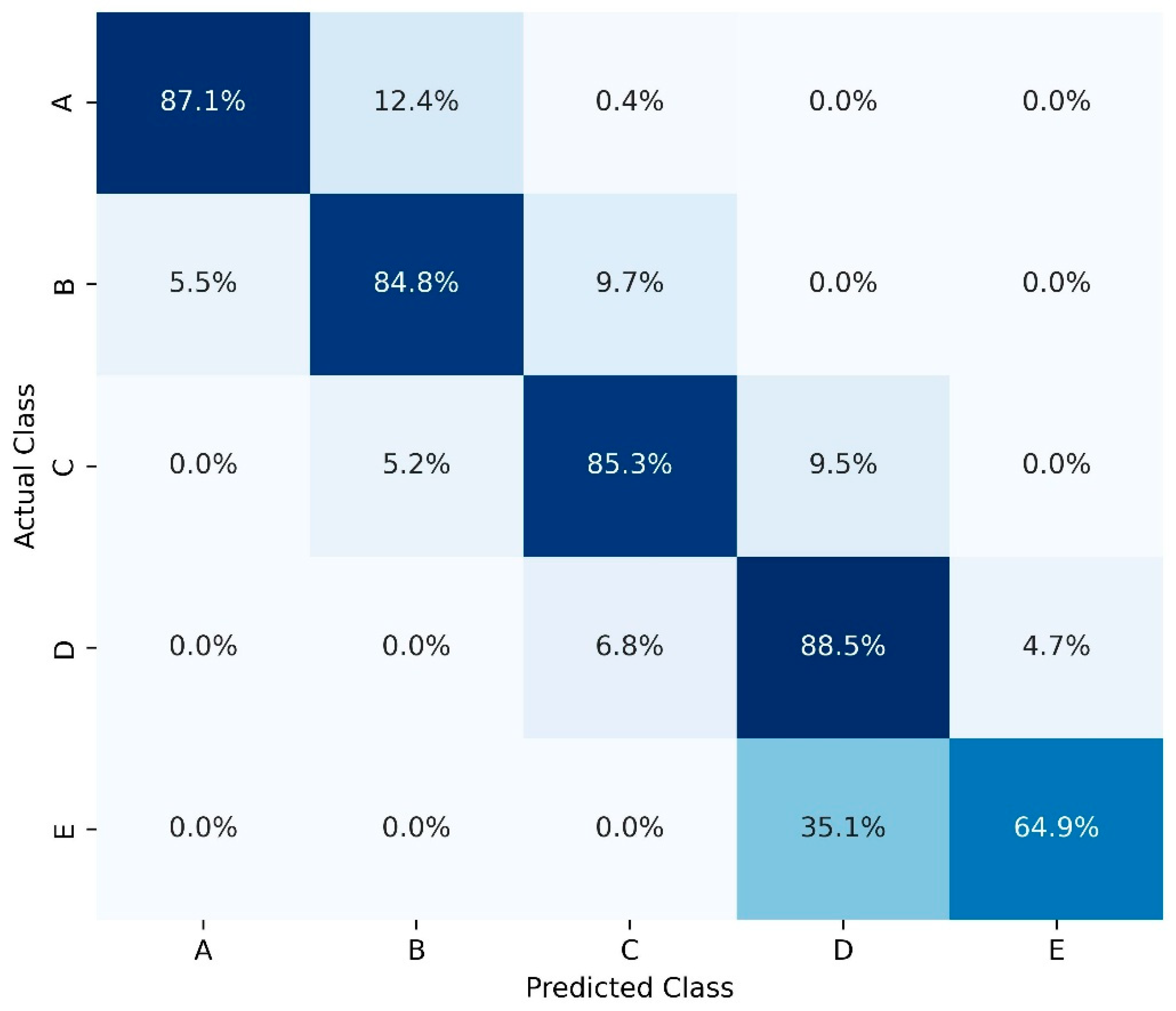
As mentioned in the results section, the three-sensor configuration was the chosen one to train the ML models, and the XGB is the model that better balances prediction capabilities with training time. Figure 11 shows the dispersion plot of the estimation results on the test set. Most of the predictions are close to the ground-truth represented by the red line. Even though we have not posed this problem as a classification problem, as we consider that regression is more informative given a continuous target variable, it is interesting to analyze the results in terms of the quality classes defined in the EN 13848-6 [4]. The RMSE slightly varies between classes; class B is the one with the lowest error, and class E is the one with the highest. As might be expected, many of the points not estimated in their actual class are those whose standard deviation values are close to the boundary between two track quality classes. The confusion matrix between classes is shown in Figure 12. It can be seen that, except for a single point classified as class C but actually belonging to class A, there are only misclassifications between adjacent classes. The consistent error and classification accuracy values observed across track quality classes indicate stable model behavior, although an increase in prediction dispersion is observed for higher target variable values, which can be attributed to the larger variability associated with poorer track qualities. This supports the effectiveness of the selected sensor configuration with respect to variations in track condition. Moreover, as the models were trained and tested using data generated from a wide and uniformly sampled parameter space, the results indicate that the models generalize well across the operating conditions covered by the simulations.

Figure 11. Comparison between the estimated and actual values of the standard deviation of longitudinal irregularities. The red solid line represents the ideal one-to-one relationship. The dashed lines indicate the limits of the quality classes (A–E) used for performance evaluation.

Figure 12. Confusion matrix for the longitudinal track quality classes. The color scale represents the classification accuracy in each cell, with darker shades indicating higher percentages.

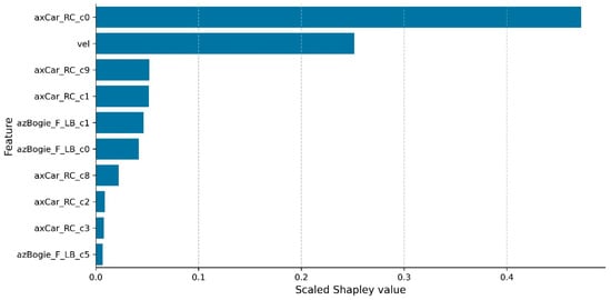
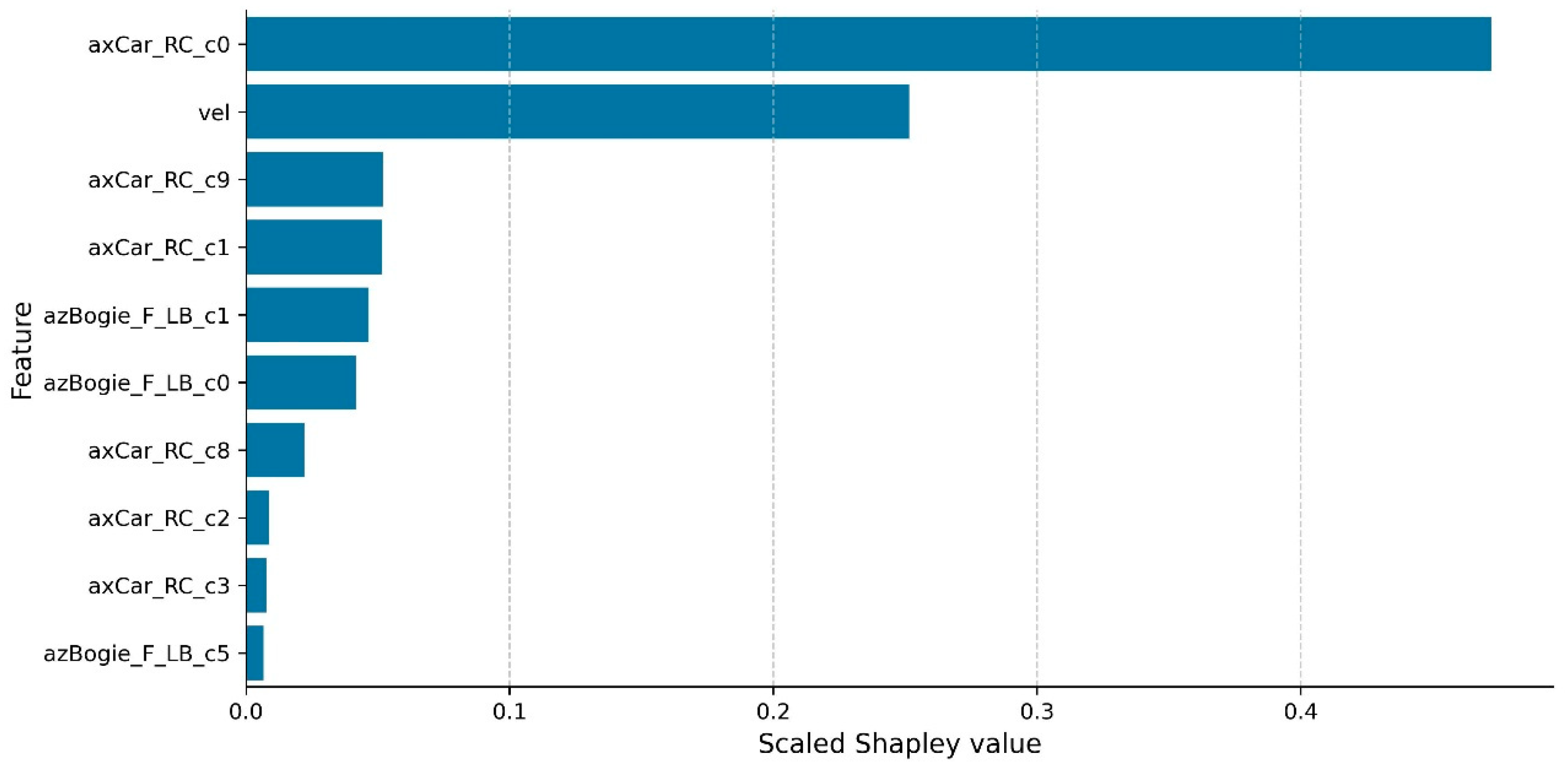
To understand which features are the most influential for estimating track longitudinal quality, Shapley values were calculated for the trained XGB model. The top 10 features with the highest global importance are shown in Figure 13. This analysis reveals that the model is primarily driven by the first principal component of the longitudinal acceleration of the car-body and the vehicle speed. In contrast, features extracted from the bogie exhibit comparatively lower Shapley values.

Figure 13. Scaled Shapley values of extracted features.

These findings stand in apparent contrast to the sensor selection results in Table 3, which shows that the best-performing two-sensor combination includes the vertical acceleration of the bogie instead of the car-body. However, this can be explained by the high correlation (above 0.90) between the first principal components extracted from both signals. This relationship indicates that both signals encode substantially similar information regarding the track profile. Consequently, in the three-sensor configuration, the model treats them as redundant and assigns primary importance to the car-body signals.

The absolute value of the correlation between other components is below 0.3, suggesting they contribute distinct, non-redundant information. In conclusion, vehicle speed and the first principal components contribute to the bulk of predictions, while higher-order components are employed to refine them.

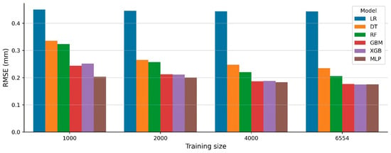
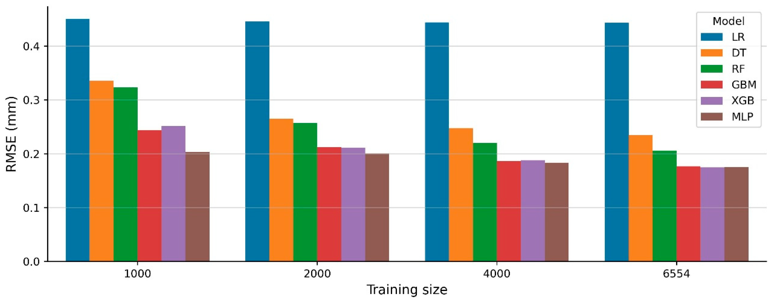
Simulations are computationally expensive, and real-world data may be sparse or unbalanced. As a consequence, the amount of available training data is a limiting factor to consider. Figure 14 shows the error achieved by the different models in the test dataset depending on the size of the training set. Since more data is needed to correctly model non-linear dependences, all models notably improve with more training data except for the linear regression model. Among the best models, XGB is the most sensitive to data scarcity and MLP, the least. The improvement in the models from a training size of 4000 to 6554 is minor, suggesting that 6554 samples are sufficient for this problem. Further data collection would likely yield diminishing returns.

Figure 14. Models error as a function of the training dataset size.

In summary, the presented results highlight the balance achieved between predictive accuracy and physical interpretability within our methodology. By integrating a sensor selection strategy with standard regression models, the proposed framework proves to be both computationally lightweight and data-efficient for estimating longitudinal track quality. Synthetic data constitute the backbone of the approach, as they allow a systematic exploration of a large number of sensor locations, which is impractical in a real vehicle. Moreover, simulation data can be used to complement real-world datasets, where unhealthy track conditions are typically scarce in operational lines. Although the current study is validated using simulated data, the results demonstrate the ability of the methodology to capture the essential dynamics of vehicle–track interaction and to extract informative patterns for track quality estimation. In real-world applications, differences between simulated and measured data are expected due to noise, installation effects, and unmodeled phenomena. Addressing this domain gap constitutes a natural next step.

The employed MBS model of the regional vehicle is based on mechanical characteristics provided for a common, in-service vehicle series. In future work, the proposed methodology is intended to be validated against field measurements. The optimal sensor configuration reported in this study can be transferred to the real system when the objective is the estimation of longitudinal level quality. However, we recommend incorporating any prior information and constraints available about the vehicle and operating conditions into the simulation model and the optimization algorithm to obtain a more focused sensor configuration. Given their data-driven nature, the ML models must be retrained and validated with real data to meet the reliability requirements. Depending on the availability, quantity, and variability of measured data, different strategies can be adopted. For vehicles substantially different from the simulated regional case (e.g., metro systems or high-speed trains), transfer learning or domain adaptation techniques can be applied to adapt models trained in simulation to new operating regimes. For regional vehicles comparable to the one considered here, the MBS model itself can be refined and fitted to the specific vehicle configuration, after which the complete methodology can be replicated to ensure consistency. In addition, simulation data and field measurements may be combined during model training to leverage the complementary advantages of both sources: using synthetic data to cover conditions that are uncommon in practice, and measured data to anchor the models to real-world behavior. In this sense, the present work establishes a flexible foundation for future validation and deployment under real operating conditions.

5. Conclusions

An end-to-end methodology for the development of track quality estimation systems based on onboard inertial sensors has been presented and evaluated under simulated conditions. The methodology integrates experimental design, signal processing, sensor selection, and machine learning-based estimation within a unified framework and was specifically implemented for longitudinal-level track quality estimation. A root mean squared error of 0.175 mm was obtained on the test dataset. The main contributions and conclusions of this work are as follows:

• The methodology developed provides a systematic framework encompassing the entire process from data acquisition to the construction of track quality estimation models. This approach integrates key elements such as experimental design and sensor selection, allowing decisions to be informed by shared data and performance metrics.
• A sensor selection strategy has been designed based on multi-objective optimization to find a sensor layout that balances track quality estimation accuracy and the number of required sensors. Vertical and longitudinal accelerations on the bogie frames and car-body, along with vehicle speed, were found to be the most informative signals, while other combinations yielded comparable performance, and additional factors, such as installation feasibility, must also be considered.
• Although the focus was on improving the formulation of the problem itself, promising results have been obtained. Gradient Boosting Machine, XGBoost, and Multilayer Perceptron models yielded similar accuracy on the test dataset. Nevertheless, the average training time of XGBoost was more than one order of magnitude lower than that of the other models. Thus, XGBoost was employed throughout the entire workflow of the methodology due to its superior training speed and overall computational efficiency.
• The principal components of the wavelet spectra of the generated signals were used as predictor variables. We found that these features outperformed statistical measures traditionally used for track quality estimation, reducing the RMSE from 0.229 to 0.175 mm.

While the specific sensor layouts and error values are context-dependent, the proposed methodology is transferable across vehicles and operating conditions. Future work will address the estimation of additional track quality indices, such as alignment track quality, and the validation of the methodology under real operational conditions, which will require the application of domain adaptation and transfer learning strategies.

Appendix A.1. List of Utilized Sensors

In Table A1, sensors defined in the simulation model and employed in this study are listed and their location is described. Suffixes ax, ay, and az are added to the sensor identifier to specify its orientation: longitudinal, lateral or vertical, respectively.

Table A1. Glossary of sensors used.

Sensor Identifier	Location Description
Car_FL	Front left of car-body floor
Car_FC	Front center of car-body floor
Car_FR	Front right of car-body floor
Car_CL	Centre left of car-body floor
Car_CC	Centre center of car-body floor
Car_CR	Centre right of car-body floor
Car_RL	Back left of car-body floor
Car_RC	Back center of car-body floor
Car_RR	Back right of car-body floor
Bogie_F_LF	Front left of frontal bogie frame
Bogie_F_LB	Back left of frontal bogie frame
Bogie_F_RF	Front right of frontal bogie frame
Bogie_F_RB	Back right of frontal bogie frame
Bogie_R_LF	Front left of rear bogie frame
Bogie_R_LB	Back left of rear bogie frame
Bogie_R_RF	Front right of rear bogie frame
Bogie_R_RB	Back right of rear bogie frame
WS1_L	Left axle box of first wheel set
WS1_R	Right axle box of first wheel set
WS2_L	Left axle box of second wheel set
WS2_R	Right axle box of second wheel set
WS3_L	Left axle box of third wheel set
WS3_R	Right axle box of third wheel set
WS4_L	Left axle box of fourth wheel set
WS4_R	Right axle box of fourth wheel set

Table A1. Glossary of sensors used.

Sensor Identifier	Location Description
Car_FL	Front left of car-body floor
Car_FC	Front center of car-body floor
Car_FR	Front right of car-body floor
Car_CL	Centre left of car-body floor
Car_CC	Centre center of car-body floor
Car_CR	Centre right of car-body floor
Car_RL	Back left of car-body floor
Car_RC	Back center of car-body floor
Car_RR	Back right of car-body floor
Bogie_F_LF	Front left of frontal bogie frame
Bogie_F_LB	Back left of frontal bogie frame
Bogie_F_RF	Front right of frontal bogie frame
Bogie_F_RB	Back right of frontal bogie frame
Bogie_R_LF	Front left of rear bogie frame
Bogie_R_LB	Back left of rear bogie frame
Bogie_R_RF	Front right of rear bogie frame
Bogie_R_RB	Back right of rear bogie frame
WS1_L	Left axle box of first wheel set
WS1_R	Right axle box of first wheel set
WS2_L	Left axle box of second wheel set
WS2_R	Right axle box of second wheel set
WS3_L	Left axle box of third wheel set
WS3_R	Right axle box of third wheel set
WS4_L	Left axle box of fourth wheel set
WS4_R	Right axle box of fourth wheel set

Appendix A.2. Machine Learning Models Hyperparameters

Table A2. Decision Tree hyperparameters.

Parameter	Final Value	Tuning Range	Description
splitter	“best”	“best”, “random”	The strategy used to choose the split at each node.
max_depth	15	3–20	The maximum depth of the tree.
min_samples_split	7	2–20	The minimum number of samples a node must have before it can be split.
min_samples_leaf	12	1–20	The minimum number of samples required to be at a leaf node.

Table A2. Decision Tree hyperparameters.

Parameter	Final Value	Tuning Range	Description
splitter	“best”	“best”, “random”	The strategy used to choose the split at each node.
max_depth	15	3–20	The maximum depth of the tree.
min_samples_split	7	2–20	The minimum number of samples a node must have before it can be split.
min_samples_leaf	12	1–20	The minimum number of samples required to be at a leaf node.

Table A3. Random Forest hyperparameters.

Parameter	Final Value	Tuning Range	Description
n_estimators	241	1–300	The number of trees in the forest.
max_depth	14	3–20	The maximum depth of each tree.
min_samples_split	6	2–20	The minimum number of samples of a node must be split.
min_samples_leaf	3	1–20	The minimum number of samples required at a leaf node.

Table A3. Random Forest hyperparameters.

Parameter	Final Value	Tuning Range	Description
n_estimators	241	1–300	The number of trees in the forest.
max_depth	14	3–20	The maximum depth of each tree.
min_samples_split	6	2–20	The minimum number of samples of a node must be split.
min_samples_leaf	3	1–20	The minimum number of samples required at a leaf node.

Table A4. Gradient Boosting Machine hyperparameters.

Parameter	Final Value	Tuning Range	Description
n_estimators	275	50–300	The number of boosting stages (trees) to perform.
learning_rate	0.044	0.01–0.3	Parameter to shrink the contribution of each tree.
max_depth	13	3–16	The maximum depth of a tree
min_samples_split	10	2–20	The minimum samples required to split an internal node.
max_samples_leaf	16	1–20	The minimum samples required at a leaf node.
subsample	0.551	0.5–1.0	The fraction of samples to be used for fitting each base learner.

Table A4. Gradient Boosting Machine hyperparameters.

Parameter	Final Value	Tuning Range	Description
n_estimators	275	50–300	The number of boosting stages (trees) to perform.
learning_rate	0.044	0.01–0.3	Parameter to shrink the contribution of each tree.
max_depth	13	3–16	The maximum depth of a tree
min_samples_split	10	2–20	The minimum samples required to split an internal node.
max_samples_leaf	16	1–20	The minimum samples required at a leaf node.
subsample	0.551	0.5–1.0	The fraction of samples to be used for fitting each base learner.

Table A5. XGBoost hyperparameters.

Parameter	Final Value	Tuning Range	Description
num_boost_round	1782	300–2000	The number of boosting rounds (trees) to perform.
learning_rate	0.018	0.01–0.3	Parameter to shrink the contribution of each tree.
max_depth	5	3–16	The maximum depth of a tree.
subsample	0.590	0.5–1.0	The fraction of samples to be used for fitting each base learner.
colsample_bytree	0.913	0.5–1.0	The fraction of features to be used for fitting each base learner.

Table A5. XGBoost hyperparameters.

Parameter	Final Value	Tuning Range	Description
num_boost_round	1782	300–2000	The number of boosting rounds (trees) to perform.
learning_rate	0.018	0.01–0.3	Parameter to shrink the contribution of each tree.
max_depth	5	3–16	The maximum depth of a tree.
subsample	0.590	0.5–1.0	The fraction of samples to be used for fitting each base learner.
colsample_bytree	0.913	0.5–1.0	The fraction of features to be used for fitting each base learner.

Table A6. Multilayer Perceptron hyperparameters.

Parameter	Final Value	Tuning Range	Description
num_hidden_layers	3	1–4	Number of hidden layers.
hidden_layer_sizes	(180, 175, 45)	10–200	A tuple specifying the number of neurons in each hidden layer.
activation	“ReLU”	“ReLU”, “tanh”	The activation function for the hidden layers.
alpha	0.00370	1 × 10−5–0.1	The L2 regularization penalty parameter.
learning_rate	0.00038	1 × 10−4–0.1	The learning rate.

Table A6. Multilayer Perceptron hyperparameters.

Parameter	Final Value	Tuning Range	Description
num_hidden_layers	3	1–4	Number of hidden layers.
hidden_layer_sizes	(180, 175, 45)	10–200	A tuple specifying the number of neurons in each hidden layer.
activation	“ReLU”	“ReLU”, “tanh”	The activation function for the hidden layers.
alpha	0.00370	1 × 10−5–0.1	The L2 regularization penalty parameter.
learning_rate	0.00038	1 × 10−4–0.1	The learning rate.

References

- de Melo, A.L.O.; Kaewunruen, S.; Papaelias, M.; Bernucci, L.L.B.; Motta, R. Methods to Monitor and Evaluate the Deterioration of Track and Its Components in a Railway In-Service: A Systemic Review. Front. Built Environ. 2020, 6, 118. [Google Scholar] [CrossRef] [Scilit]
- Shi, C.; Zhou, Y.; Xu, L.; Zhang, X.; Guo, Y. A Critical Review on the Vertical Stiffness Irregularity of Railway Ballasted Track. Constr. Build. Mater. 2023, 400, 132715. [Google Scholar] [CrossRef] [Scilit]
- Vilotijević, M.; Brajović, L.; Lazarević, L.; Mirković, N. Methods for Track Stiffness Measurement-State of the Art. In Proceedings of the New Horizons, Isparta, Turkey, 18–20 October 2017. [Google Scholar]
- CEN/EN 13848–6; Railway Applications—Track—Track Geometry Quality—Part 6: Characterization of Track Geometry Quality. CEN: Brussels, Belgium, 2020.
- TB/T 3355-2014; Track Geometry Dynamic Inspection and Evaluation Method. China Railway Publishing House: Beijing, China, 2014.
- Singh, A.K. Dynamic Modeling and Ride Comfort Evaluation of Railway Vehicle under Random Track Irregularities: A Case Study of a Linke-Hofmann-Busch Coach. J. Eng. Res. 2024, 12, 984–993. [Google Scholar] [CrossRef] [Scilit]
- Xiao, X.; Xu, H.W.; Yang, Y.; Chen, P.; Hu, Q. Analysis of the Influence of Track Irregularity on High-Speed Train Ride Comfort. Veh. Syst. Dyn. 2024, 62, 1658–1685. [Google Scholar] [CrossRef] [Scilit]
- Farkas, A. Measurement of Railway Track Geometry: A State-of-the-Art Review. Period. Polytech. Transp. Eng. 2019, 48, 76–88. [Google Scholar] [CrossRef] [Scilit]
- Fernandez-Bobadilla, H.A.; Martin, U. Modern Tendencies in Vehicle-Based Condition Monitoring of the Railway Track. IEEE Trans. Instrum. Meas. 2023, 72, 1–44. [Google Scholar] [CrossRef] [Scilit]
- Weston, P.; Roberts, C.; Yeo, G.; Stewart, E. Perspectives on Railway Track Geometry Condition Monitoring from In-Service Railway Vehicles. Veh. Syst. Dyn. 2015, 53, 1063–1091. [Google Scholar] [CrossRef] [Scilit]
- Chia, L.; Bhardwaj, B.; Lu, P.; Bridgelall, R. Railroad Track Condition Monitoring Using Inertial Sensors and Digital Signal Processing: A Review. IEEE Sens. J. 2019, 19, 25–33. [Google Scholar] [CrossRef]
- Cai, X.; Tang, X.; Yang, F.; Wang, T.; Sun, J. Estimation of Turnout Irregularities Using Vehicle Responses with Improved BiLSTM and Gaussian Process Regression. Measurement 2023, 221, 113513. [Google Scholar] [CrossRef] [Scilit]
- Chen, M.; Zhai, W.; Zhu, S.; Xu, L.; Sun, Y. Vibration-Based Damage Detection of Rail Fastener Using Fully Convolutional Networks. Veh. Syst. Dyn. 2022, 60, 2191–2210. [Google Scholar] [CrossRef] [Scilit]
- Strano, S.; Terzo, M. Review on Model-Based Methods for on-Board Condition Monitoring in Railway Vehicle Dynamics. Adv. Mech. Eng. 2019, 11, 1687814019826795. [Google Scholar] [CrossRef] [Scilit]
- Sansiñena, A.; Rodríguez-Arana, B.; Arrizabalaga, S. A Systematic Review of Acceleration-Based Estimation of Railway Track Quality. Veh. Syst. Dyn. 2025, 1–28. [Google Scholar] [CrossRef] [Scilit]
- Tsunashima, H. Condition Monitoring of Railway Tracks from Car-Body Vibration Using a Machine Learning Technique. Appl. Sci. 2019, 9, 2734. [Google Scholar] [CrossRef] [Scilit]
- Liu, R.; Wang, F.-T.; Wang, Z.-P.; Wu, C.-L.; He, H.-D. Identification of Subway Track Irregularities Based on Detection Data of Portable Detector. Transp. Res. Rec. J. Transp. Res. Board 2022, 2676, 703–713. [Google Scholar] [CrossRef] [Scilit]
- La Paglia, I.; Carnevale, M.; Corradi, R.; Di Gialleonardo, E.; Facchinetti, A.; Lisi, S. Condition Monitoring of Vertical Track Alignment by Bogie Acceleration Measurements on Commercial High-Speed Vehicles. Mech. Syst. Signal Process. 2023, 186, 109869. [Google Scholar] [CrossRef] [Scilit]
- Tsunashima, H.; Yagura, N. Railway Track Irregularity Estimation Using Car Body Vibration: A Data-Driven Approach for Regional Railway. Vibration 2024, 7, 928–948. [Google Scholar] [CrossRef] [Scilit]
- Hao, X.; Yang, J.; Yang, F.; Sun, X.; Hou, Y.; Wang, J. Track Geometry Estimation from Vehicle–Body Acceleration for High-Speed Railway Using Deep Learning Technique. Veh. Syst. Dyn. 2023, 61, 239–259. [Google Scholar] [CrossRef] [Scilit]
- Yang, J.; Liu, J.; Guo, J.; Tao, K. Track Irregularity Identification Method of High-Speed Railway Based on CNN-Bi-LSTM. Sensors 2024, 24, 2861. [Google Scholar] [CrossRef] [Scilit]
- Pires, A.C.; Viana, M.C.A.; Scaramussa, L.M.; Santos, G.F.M.; Ramos, P.G.; Santos, A.A. Measuring Vertical Track Irregularities from Instrumented Heavy Haul Railway Vehicle Data Using Machine Learning. Eng. Appl. Artif. Intell. 2024, 127, 107191. [Google Scholar] [CrossRef] [Scilit]
- Odashima, M.; Azami, S.; Naganuma, Y.; Mori, H.; Tsunashima, H. Track Geometry Estimation of a Conventional Railway from Car-Body Acceleration Measurement. Mech. Eng. J. 2017, 4, 16–00498. [Google Scholar] [CrossRef] [Scilit]
- Dai, B.; Xu, Y.L.; Li, Q.; Zhang, Z. Vertical Track Irregularity Identification Based on a Physics-Informed Kolmogorov-Arnold Network with Bogie Accelerations of in-Service Trains. Mech. Syst. Signal Process. 2026, 245, 113845. [Google Scholar] [CrossRef] [Scilit]
- Chellaswamy, C.; Krishnasamy, M.; Balaji, L.; Dhanalakshmi, A.; Ramesh, R. Optimized Railway Track Health Monitoring System Based on Dynamic Differential Evolution Algorithm. Measurement 2020, 152, 107332. [Google Scholar] [CrossRef] [Scilit]
- Wei, X.; Liu, F.; Jia, L. Urban Rail Track Condition Monitoring Based on In-Service Vehicle Acceleration Measurements. Measurement 2016, 80, 217–228. [Google Scholar] [CrossRef] [Scilit]
- Ward, C.P.; Weston, P.F.; Stewart, E.J.C.; Li, H.; Goodall, R.M.; Roberts, C.; Mei, T.X.; Charles, G.; Dixon, R. Condition Monitoring Opportunities Using Vehicle-Based Sensors. Proc. Inst. Mech. Eng. F J. Rail Rapid Transit 2011, 225, 202–218. [Google Scholar] [CrossRef] [Scilit]
- Ghiasi, R.; Khan, M.A.; Sorrentino, D.; Diaine, C.; Malekjafarian, A. An Unsupervised Anomaly Detection Framework for Onboard Monitoring of Railway Track Geometrical Defects Using One-Class Support Vector Machine. Eng. Appl. Artif. Intell. 2024, 133, 108167. [Google Scholar] [CrossRef] [Scilit]
- Ghiasi, R.; Lestoille, N.; Diaine, C.; Malekjafarian, A. A Novel Domain Adaptation Method for Drive-by Railway Track Monitoring Using Progressive Distribution Alignment Based on Label Correction. Struct. Health Monit. 2025, 1–25. [Google Scholar] [CrossRef] [Scilit]
- Garud, S.S.; Karimi, I.A.; Kraft, M. Design of Computer Experiments: A Review. Comput. Chem. Eng. 2017, 106, 71–95. [Google Scholar] [CrossRef] [Scilit]
- Rulka, W. SIMPACK—A Computer Program for Simulation of Large-Motion Multibody Systems. In Multibody Systems Handbook; Springer: Berlin, Germany, 1990; pp. 265–284. [Google Scholar]
- Sobol, I.M. Uniformly Distributed Sequences with an Additional Uniform Property. USSR Comput. Math. Math. Phys. 1975, 16, 236–242. [Google Scholar] [CrossRef] [Scilit]
- Zhai, W. Vehicle–Track Coupled Dynamics; Springer: Singapore, 2020; ISBN 978-981-32-9282-6. [Google Scholar]
- Zhang, Y.; Sun, X.; Xu, X.; Dong, W.; Ji, Y. Track Irregularities Estimation Based on the Vibration of Car-Body. In Proceedings of the 2017 IEEE 2nd Advanced Information Technology, Electronic and Automation Control Conference (IAEAC); IEEE: New York, NY, USA, 2017; pp. 1369–1372. [Google Scholar]
- La Paglia, I.; Di Gialleonardo, E.; Facchinetti, A.; Carnevale, M.; Corradi, R. A Methodology to Estimate Railway Track Conditions from Vehicle Accelerations Based on Multiple Regression. In Proceedings of the Lecture Notes in Civil Engineering; Springer: Cham, Switzerland, 2023; Volume 432 LNCE, pp. 203–210. [Google Scholar]
- Li, J.; Shi, H. Rail Corrugation Diagnosis of High-Speed Railway Based on Dynamic Responses of the Vehicle. In Proceedings of the 2020 Prognostics and Health Management Conference (PHM-Besançon); IEEE: New York, NY, USA, 2020; pp. 148–152. [Google Scholar]
- Mallat, S. A Wavelet Tour of Signal Processing, 3rd ed.; Academic Press: Cambridge, MA, USA, 2009; ISBN 9780123743701. [Google Scholar]
- Ghosh, C.; Verma, A.; Verma, P. Real Time Fault Detection in Railway Tracks Using Fast Fourier Transformation and Discrete Wavelet Transformation. Int. J. Inf. Technol. 2022, 14, 31–40. [Google Scholar] [CrossRef] [Scilit]
- Galvín, P.; Romero, A.; Solís, M.; Moliner, E.; Martínez-Rodrigo, M.D. Time–Frequency Analysis of Railway Bridges Forced and Free Vibrations Identified by Wavelet Transform. Vibration 2025, 8, 71. [Google Scholar] [CrossRef] [Scilit]
- Pearson, K. LIII. On Lines and Planes of Closest Fit to Systems of Points in Space. Lond. Edinb. Dublin Philos. Mag. J. Sci. 1901, 2, 559–572. [Google Scholar] [CrossRef] [Scilit]
- Zhou, A.; Qu, B.-Y.; Li, H.; Zhao, S.-Z.; Suganthan, P.N.; Zhang, Q. Multiobjective Evolutionary Algorithms: A Survey of the State of the Art. Swarm Evol. Comput. 2011, 1, 32–49. [Google Scholar] [CrossRef] [Scilit]
- Deb, K.; Pratap, A.; Agarwal, S.; Meyarivan, T. A Fast and Elitist Multiobjective Genetic Algorithm: NSGA-II. IEEE Trans. Evol. Comput. 2002, 6, 182–197. [Google Scholar] [CrossRef] [Scilit]
- Chen, T.; Guestrin, C. XGBoost: A Scalable Tree Boosting System. In Proceedings of the 22nd ACM SIGKDD International Conference on Knowledge Discovery and Data Mining, San Francisco, CA, USA, 13–17 August 2016; ACM: New York, NY, USA, 2016; pp. 785–794. [Google Scholar]
- Hastie, T.; Tibshirani, R.; Friedman, J. The Elements of Statistical Learning; Springer Series in Statistics; Springer: New York, NY, USA, 2009; ISBN 978-0-387-84857-0. [Google Scholar]
- Bergstra, J.; Bardenet, R.; Bengio, Y.; Kégl, B. Algorithms for Hyper-Parameter Optimization. In Proceedings of the Advances in Neural Information Processing Systems; Curran Associates, Inc.: Red Hook, NY, USA, 2011; Volume 24. [Google Scholar]
- Lundberg, S.; Lee, S.-I. A Unified Approach to Interpreting Model Predictions. In Proceedings of the Advances in Neural Information Processing Systems; Curran Associates, Inc.: Red Hook, NY, USA, 2017; Volume 30. [Google Scholar]
- Akiba, T.; Sano, S.; Yanase, T.; Ohta, T.; Koyama, M. Optuna: A Next-generation Hyperparameter Optimization Framework. In Proceedings of the 25th ACM SIGKDD International Conference on Knowledge Discovery & Data Mining; ACM: New York, NY, USA, 2019; pp. 2623–2631. [Google Scholar]
- Paszke, A.; Gross, S.; Massa, F.; Lerer, A.; Bradbury, J.; Chanan, G.; Killeen, T.; Lin, Z.; Gimelshein, N.; Antiga, L.; et al. PyTorch: An Imperative Style, High-Performance Deep Learning Library. In Proceedings of the Advances in Neural Information Processing Systems; Curran Associates, Inc.: Red Hook, NY, USA, 2019; Volume 32. [Google Scholar]
- Pedregosa, F.; Michel, V.; Grisel, O.; Blondel, M.; Prettenhofer, P.; Weiss, R.; Vanderplas, J.; Cournapeau, D.; Varoquaux, G.; Gramfort, A.; et al. Scikit-Learn: Machine Learning in Python. J. Mach. Learn. Res. 2011, 12, 2825–2830. [Google Scholar]
- Dumitriu, M. Analysis of the Dynamic Response in the Railway Vehicles to the Track Vertical Irregularities. Part II: The Numerical Analysis. J. Eng. Sci. Technol. Rev. 2015, 8, 32–39. [Google Scholar] [CrossRef] [Scilit]
Disclaimer/Publisher’s Note: The statements, opinions and data contained in all publications are solely those of the individual author(s) and contributor(s) and not of MDPI and/or the editor(s). MDPI and/or the editor(s) disclaim responsibility for any injury to people or property resulting from any ideas, methods, instructions or products referred to in the content. |
© 2026 by the authors. Licensee MDPI, Basel, Switzerland. This article is an open access article distributed under the terms and conditions of the Creative Commons Attribution (CC BY) license.