


Abstract
This study implements a hybrid unsupervised machine learning approach for detecting anomalies in electricity consumption patterns from Advanced Metering Infrastructure (AMI) systems. The proposed methodology integrates dimensionality reduction techniques using Principal Component Analysis (PCA) with the Hierarchical Density-Based Spatial Clustering of Applications with Noise (HDBSCAN) algorithm to identify anomalous behavior. The dataset, which encompasses 26,230 m and spans a one-year period, is segmented based on user type for the purpose of analysis. The findings indicate a high degree of temporal stability in residential consumption patterns, with detection performance varying depending on the nature of the simulated anomaly. The “Sudden Drop” anomaly pattern shows an average detection rate of 61%, with monthly peaks reaching up to 96%, while more subtle anomalies such as flattening remain considerably harder to identify, with detection rates ranging between 4% and 35%. These findings contribute to the development of automated surveillance systems for reducing non-technical losses in electrical distribution networks.
1. Introduction
The growth of smart grids has fundamentally transformed the management and monitoring of electricity consumption by incorporating smart meters, advanced communication infrastructure, and big data analytics platforms. This digital ecosystem generates large volumes of real-time information that improve operational efficiency and the integration of renewable energies, but it also introduces new challenges related to the detection of outliers that can compromise the security and reliability of the system [1,2].
In this context, outliers represent not only extreme statistical values but also phenomena such as measurement errors, abnormal operating conditions, fraud, and non-technical losses [3,4,5], as well as cyberattacks and intrusions into the digitized infrastructure of networks [6,7]. Recognizing and properly classifying these anomalies is essential to differentiate between transient noise and critical events that require immediate intervention, with load profile characterization being a key tool in this task [8]. In turn, the increased use of smart grids allows for greater data governance, making it possible not only to identify potential outliers and fraud, but also to monitor high energy consumption in pursuit of efficiency and sustainability.
The literature shows a transition from classical heuristic and statistical approaches to artificial intelligence methodologies in which models such as LSTM, GRU, autoencoders, and graph-based neural networks (GNN/GCN) are able to capture complex spatiotemporal patterns with greater accuracy than traditional techniques such as PCA or k-means [9,10,11,12]. These approaches make it possible to identify both isolated anomalies and persistent anomalous patterns that can affect network stability.
Complementarily, several studies propose integrating forecasting models with anomaly detectors based on residuals, enabling hybrid schemes capable of anticipating irregular behavior [13,14]. This is particularly relevant in scenarios with high penetration of renewables and electric vehicles, where demand variability increases the probability of atypical events [15]. At the same time, federated learning initiatives and privacy preservation techniques are emerging that seek to balance the effectiveness of algorithms with compliance with regulations on the handling of sensitive data [2,16].
The detection of outliers in electrical networks is an interdisciplinary field with a high practical impact. Developments in this area contribute not only to the safe and reliable operation of systems, but also to loss management and fraud prevention [3], as well as defense against cyber threats [5]. Recent advances in data imputation and deep learning have shaped a new generation of solutions that can transform the way energy companies and regulators address the challenges of the energy transition [17,18].
Existing approaches for anomaly detection in electricity consumption data can be broadly categorized into four main groups: (i) classical statistical methods, (ii) clustering and density-based techniques, (iii) machine learning and deep learning approaches, and (iv) hybrid and alternative methods. Each category offers different trade-offs in terms of interpretability, scalability, computational cost, and data requirements. These categories differ not only in their modeling capabilities but also in their practical applicability to large-scale AMI datasets.
Classical statistical methods are widely used due to their interpretability and low computational cost; however, they often struggle to capture nonlinear consumption patterns and complex temporal dependencies [19]. Clustering and density-based approaches enable the identification of anomalous patterns without requiring labeled data, making them suitable for large-scale AMI datasets, although their performance depends on the underlying data distribution and parameter selection. Machine learning and deep learning models, such as LSTM networks and autoencoders, have demonstrated strong capabilities in modeling complex temporal behavior, but they typically require large datasets and significant computational resources. Hybrid approaches aim to combine the strengths of multiple techniques to improve robustness and detection accuracy, although they may introduce additional complexity in model design and calibration.
In this context, the proposed PCA–HDBSCAN framework can be positioned within the category of hybrid unsupervised methods, as it combines dimensionality reduction with density-based clustering to leverage the strengths of both approaches. By integrating PCA and HDBSCAN, the methodology aims to provide a balance between interpretability, scalability, and the ability to detect complex consumption patterns without requiring labeled data, addressing some of the limitations identified in existing approaches.
Despite the advantages offered by these approaches, several practical limitations remain. Deep learning models, such as LSTM networks and autoencoders, are capable of capturing complex temporal dependencies but typically require large labeled datasets and significant computational resources, which limits their applicability in large-scale AMI systems. On the other hand, simpler clustering methods such as k-means provide computational efficiency but are sensitive to initialization and assume simplified cluster structures that may not reflect the true geometry of electricity consumption patterns. Furthermore, many existing approaches struggle to simultaneously provide interpretability, scalability, and robustness when dealing with high-dimensional and unlabeled consumption data.
In this context, there is a need for methodologies that can effectively detect anomalous patterns without relying on labeled data, while maintaining computational efficiency and interpretability. As summarized in Table 1, existing approaches present trade-offs in terms of data requirements, interpretability, and computational cost. The proposed PCA–HDBSCAN approach addresses this gap by combining dimensionality reduction with a density-based clustering method capable of identifying clusters of varying shapes and densities, while naturally detecting anomalous observations as noise points.
Table 1.
Comparison of anomaly detection methods and their characteristics.
This paper is organized into eight main sections. First, the introduction presents the motivation and contributions of the research. Second, the nomenclature section is introduced. Third, the literature review discusses outlier detection and analysis methods, highlighting both classical and machine learning approaches that have shown strong performance in detection tasks. Fourth, the methodology is described. Fifth, the data used in the study are presented. Sixth, the results are reported, along with performance metrics and validation using synthetic data. Seventh, the discussion is developed, and finally, eighth, the conclusions are presented.
2. Nomenclature
2.1. Acronyms and Abbreviations
AE: Autoencoder.
AIC: Akaike Information Criterion.
AMI: Advanced Metering Infrastructure.
BIC: Bayesian Information Criterion.
BOCPD: Bayesian Online Change Point Detection.
CUSUM: Cumulative Sum Control Chart.
DAE: Denoising Autoencoder.
DBSCAN: Density-Based Spatial Clustering of Applications with Noise.
DTW: Dynamic Time Warping.
EWMA: Exponentially Weighted Moving Average.
GMM: Gaussian Mixture Model.
GNN/GCN: Graph Neural Network/Graph Convolutional Network.
GRU: Gated Recurrent Unit.
HDBSCAN: Hierarchical Density-Based Spatial Clustering of Applications with Noise.
ICA: Independent Component Analysis.
IQR: Interquartile Range.
KDE: Kernel Density Estimation.
LOF: Local Outlier Factor.
LSTM: Long Short-Term Memory.
MAD: Median Absolute Deviation.
OPTICS: Ordering Points To Identify the Clustering Structure.
PCA: Principal Component Analysis.
PR@k: Precision at top-k.
PU Learning: Positive–Unlabeled Learning.
RBF: Radial Basis Function.
RPCA: Robust Principal Component Analysis.
SAX: Symbolic Aggregate approximation.
SPE (Q residual): Squared Prediction Error.
TCN: Temporal Convolutional Network.
THD: Total Harmonic Distortion.
VAE: Variational Autoencoder.
2.2. Variables and Symbols
: Cluster label ( = −1 indicates noise/anomaly) [–].
: Original hourly consumption [kWh].
: Transformed hourly consumption (synthetic anomaly) [kWh].
: Mean hourly profile [kWh].
: Random noise term [kWh].
: Mean daily consumption [kWh].
: Standard deviation of daily consumption [kWh].
: Reduction factor (partial bypass anomaly) [–].
: Smoothing factor [–].
: Extreme reduction factor (sudden drop anomaly) [–].
: Noise scaling factor [–].
: Principal components (PCA) [–].
2.3. Derived Variables/Features
hourP_0–hourP_23: Average consumption per hour of the day [kWh].
Median: Median daily consumption [kWh].
Max/Min: Maximum and minimum daily consumption [kWh].
Outlier score: Anomaly score produced by HDBSCAN [–].
2.4. Metrics and Statistical Concepts
Hotelling’s : Multivariate statistic used in PCA [–].
Q residual (SPE): Reconstruction error in PCA [–].
Jaccard index: Cluster stability metric [–].
Noise ratio: Proportion of points classified as noise [%].
Detection rate: Proportion of anomalies correctly detected [%].
Alert rate: Proportion of users flagged as suspicious [%].
2.5. Additional Terms
Load profile: Electricity consumption pattern over time.
Outlier: Atypical observation or behavior.
Smart grid: Digitized electricity network with monitoring capabilities.
Synthetic anomalies: Artificially generated anomalous patterns.
Temporal stability: Consistency of behavior over time.
Note: [–] denotes dimensionless quantities.
3. Outlier Detection and Analysis Methods Applied to Cundinamarca Department, Colombia
The detection of outliers in electrical networks has become a crucial field of research driven by the growth of advanced metering systems and the increasing complexity of smart grids. The large volumes of data generated by smart meters offer a unique opportunity to understand consumption patterns and improve system efficiency, but they also require tools capable of identifying when behavior is anomalous and requires special attention [18].
Throughout the literature, different approaches have been consolidated that seek to respond to this challenge from complementary perspectives. On the one hand, classical statistical methods rely on simple and transparent models that allow for quick and easy-to-interpret results [15]. On the other hand, clustering and unsupervised learning methods offer the possibility of discovering hidden patterns in the data without the need for labels, which is particularly relevant in contexts where reference information is scarce [22].
More recently, models based on neural networks and deep learning have emerged as a powerful alternative for capturing complex dependencies and spatio-temporal relationships in the power grid [6]. In addition, alternative methods have been proposed that include Bayesian, semi-supervised, and federated strategies, which seek to address emerging challenges such as scalability, privacy, and explainability [16].
3.1. Classical Statistical Methods
Classical statistical approaches base outlier detection on assumptions about data distributions and robust statistical measures. Common practices include robust z-scores (MAD/Hampel), quantile rules and dynamic bands, as well as control charts (EWMA/CUSUM) to identify sustained deviations in active/reactive energy and power factor series [15]. Their appeal lies in their interpretability and low computational cost, valuable features for operators with computing constraints or who require auditable decisions [20].
PCA remains a central tool for multivariate electrical data: it projects data into subspaces of dominant variability and uses statistics such as Hotelling’s T2 and the Q residual to flag anomalous observations. Applied to hourly profiles and P–Q vectors, it allows atypical consumption “patterns” to be isolated and regime changes to be detected [15]. In substation assets, PCA/ICA variants help highlight sensor or transformer degradation based on signatures in the latent space [21].
In this study, PCA is specifically applied to normalized hourly consumption profiles derived from smart meter data. The normalization step transforms absolute consumption values into proportional load shapes, allowing the analysis to focus on temporal usage patterns rather than consumption magnitude. Following dimensionality reduction, the first five principal components are retained, capturing the majority of the variance of the hourly profile while reducing redundancy among the 24 hourly variables. This representation enables efficient clustering in a lower-dimensional feature space while preserving the most informative characteristics of electricity consumption behavior
Methods based on density or parametric fitting (KDE, GMM) model the empirical distribution of profiles and declare outliers in low-probability regions. In environments with a mix of daily/weekly patterns, Gaussian mixture approaches with component selection capture subpopulations (e.g., residential/commercial segments) and allow for component-specific thresholds [20]. The choice of bandwidth in KDE and the number of components in GMM are critical; cross-validation practices and information criteria (AIC/BIC) help avoid overfitting [15].
In time series, the residual-based forecasting paradigm identifies anomalies when the prediction error exceeds bands that incorporate uncertainty. Classically, this includes ARIMA/ETS with intervals, and in modern terms, bands obtained from deep models or in federated frameworks where privacy is preserved [13]. Threshold calibration using hourly–daily–seasonal condition-based percentiles limits false alarms in highly seasonal contexts and has proven effective with volatile loads and renewable energy penetration [14].
Evaluation in unbalanced scenarios prioritizes metrics such as precision–recall, average precision, and PR@k (top-k alerts) in addition to time-to-detect for transient events [15,24]. In deployment, it is key to separate detection (continuous score) from decision (dynamic threshold) and to maintain recalibration in the face of concept drift; classical methods serve well as baselines and as explainable modules that complement more complex detectors [20].
3.2. Methods Based on Artificial Intelligence
K-means and variants (mini-batch, k-medoids) are used to profile typical “load patterns” (daily/weekly) and measure the distance to the centroid as an anomaly score [25]. Their simplicity and speed make them useful as pattern compressors and detectors of “global” outliers [18]. Extensions with automatic k selection and intelligent restarts reduce sensitivity to initialization and better handle multiple seasonalities [20]. In operation, mini-batch k-means allows streaming updates with low latencies [26].
Density-based methods such as DBSCAN/HDBSCAN/OPTICS detect outliers as points in low-density regions, which is ideal for rare patterns and unbalanced aggregates. They are especially effective in AMI data with multiple consumption modes and the presence of noise [22]. Distributed/hierarchical DBSCAN designs allow scaling to millions of readings and segmentation by feeder or zone while maintaining spatial consistency and memory limits [23]. Daily load profiles (DLPs) embedded with DTW/shape-based distances and then passed to HDBSCAN improve sensitivity to consumption morphologies [26].
Other unsupervised detectors include Isolation Forest, One-Class SVM, and Local Outlier Factor (LOF), which rely on the ease of isolating rare points, single class boundaries, or local k-NN density, respectively. In multimodal loads, combining LOF with shape embeddings (e.g., SAX/shapelets) provides signals of local rarity that are often lost with k-means [20]. The selection of hyperparameters (contamination, ν, k) is guided by temporal validation and PR curves under pseudo-labeling of historical anomalies [18].
Self-supervised learning approaches (e.g., contrastive pretext tasks, temporal masking) generate representations that are then fed into clustering or density-based detectors. When data is massive and unlabeled, these pretexts stabilize performance and accelerate the convergence of lightweight models [18]. In addition, hybrid pipelines first apply clustering to build groups by behavior and then calibrate specific detectors within each group to reduce the false alarm rate [20].
In non-technical losses, unsupervised or semi-supervised learning (e.g., positive–unlabeled) stands out because reliable labels are scarce. Historical profiles and consistency with “peer neighbors” are exploited to prioritize field inspections [3]. By combining density/clustering with contextual signals (business hours, local seasonality), better accuracy has been observed in actual inspection campaigns [4,6]. RNNs (LSTM/GRU) and TCNs model long- and short-term dependencies and are used in two ways: (i) as predictors that elevate residuals to anomaly scores and (ii) as direct classifiers of deviant patterns [9]. In substations and IEC-61850 buses, LSTM/TCN have shown advantages in detecting anomalous transients and atypical event sequences [10,11]. Calibration with predictive intervals or quantile loss controls false alarm rates in volatile conditions [8].
Autoencoders (AE/VAE/DAE) learn reconstructions of “normal” profiles and use the reconstruction error as a score. Variants with custom shape-based loss functions (e.g., derivative weighting, shape losses) and energy constraints improve sensitivity to subtle anomalies [18]. In cybersecurity and network telemetry contexts, deep AEs serve as noise filters and detectors of inconsistencies in flows and payloads [27]. In some deployments, AEs combined with density-based detection (e.g., GMM in latent space) outperform standalone AEs in accuracy under drift [2].
Spatial-temporal modeling with GNN/GCN incorporates network topology (electrical neighborhood and flow paths) and allows for the detection of contextual anomalies: behaviors that are marginally normal but inconsistent with electrical neighbors [1]. In practice, graphs per feeder or circuit feed graph convolutional and temporal aggregation layers; when combined with reconstruction or forecasting modules, the resulting detectors improve the precision-recall ratio compared to purely temporal approaches [8]. Integrations with hybrid pipelines (AE/GNN + DBSCAN embedding) facilitate interpretable alert triage [2].
There is a trend toward ensembles: prediction (LSTM/TCN) + reconstruction (AE/VAE) + density/clustering with aggregation of scores normalized by time context and exogenous conditions (temperature, calendar) [18]. This design reduces dependencies on a single inductive bias and is more robust to domain drift. In industrial systems, knowledge distillation and quantization allow networks to be run at the edge (gateways/meters) without sacrificing too much performance [20].
3.3. Alternative Methods
Bayesian probabilistic models (e.g., Bayesian Online Change Point Detection) and conformal prediction offer explicit error controls for detection under uncertainty, which are useful when the cost of false alarms is asymmetric. When integrated over forecast residuals, they enable calibrated online decisions [15]. In topological scenarios, graph signal processing and robust decomposition methods (subspace/sparse representations) support the separation of background structure and outliers in load matrices/tensors, providing physical interpretability [20].
Detection by motifs/shapelets and DTW-motifs identifies rare subsequences in load curves. Combined with local density (LOF/DBSCAN), it delivers comprehensible rules such as “an unusual nighttime plateau appears” [26]. When the operating distribution changes (DER/VE), drift detectors (KS/MMD/ADWIN) enable threshold recalibration and retraining cycles, maintaining the stability of the alert system [14]. For assets, simplified physical models (efficiency curves, impedances, thermal limits) generate specific checks that complement data detectors [21].
In fraud/NTL, semi-supervised and positive–unlabeled methodologies integrate structural signals (neighboring peers, comparison with peer groups) with unsupervised scores to prioritize cases for inspection. Improvements in precision@k and field campaign outcomes have been reported [3,4]. In addition, there have been advances in transfer/zero-shot learning to generalize detectors across areas with different customer mixes, reducing local labeling costs [20]. In cybersecurity, alternative approaches inspired by intrusion detection complement operational monitors [27].
Federated learning/privacy also enables alternative patterns of collaboration between companies/areas, preserving sensitive data while sharing models or embeddings. Vertical and horizontal designs combine generalization benefits without violating data policies [13,16]. The incorporation of explainability (temporal attribution, neighbor contribution in GNN) facilitates the regulatory and operational adoption of these methods [2].
Finally, in deployment, alternative pipelines prioritize operability: alert triage, context enrichment (weather, calendar), and human feedback that converts alerts into training data for future iterations. This human-in-the-loop approach bridges the gap between algorithmic detection and action in the field and integrates well with classic diagnostic modules [15]. Taken together, these alternative methods do not replace the main ones but complement them in terms of robustness, explainability, and compliance. Table 2 presents a comparative summary of these methods.
Table 2.
Extended comparative table of techniques for detecting outliers in electrical networks.
The study of detection methods has shown significant advances, but their true potential depends on the quality and type of data used. A first challenge is to define which characteristics of electrical profiles are most informative. Various studies agree that it is not enough to measure the absolute magnitude of consumption: it is necessary to differentiate between the normalized shape of the curve, which reveals consumption habits, and the raw magnitude, which reflects energy intensity. The combination of both views, together with the hourly power factor that integrates the relationship between active and reactive energy, has proven essential for characterizing behaviors and highlighting anomalies [18,28]. On the other hand, temporal granularity is also decisive, as hourly or minute-by-minute resolutions allow peaks and seasonality to be captured that are lost with overly aggregated series. Likewise, incorporating the calendar context (weekday, weekend, holiday) enriches detection, since the rarity of a pattern depends on the day on which it occurs [29].
Another critical aspect is the selection of similarity metrics. In time profile clustering scenarios, conventional distances such as Euclidean distances are often insufficient when peaks shift over time. In contrast, techniques such as Dynamic Time Warping (DTW) or k-sliding variants better capture consumption morphology even in the presence of noise, imbalance, and outliers [30,31]. Similarly, robust measures such as correntropy have been proposed as alternatives capable of maintaining sensitivity in highly variable contexts [32,33]. Additionally, the use of profile prototypes allows large user populations to be represented with a small set of typical patterns, facilitating the detection of relevant deviations [34].
Multivariate data. Power, current, voltage, and external factors (temperature, network topology) series are often incomplete or outdated, requiring imputation techniques and representations that preserve spatial and temporal consistency. A promising approach is to represent the system as an electrical graph where each node corresponds to a meter or substation and the edges reflect physical flow relationships, allowing contextual anomalies to be detected [6]. In transmission and power quality, spectral characteristics (harmonics, distortions, THD) have proven to be fundamental in identifying invisible anomalies in the aggregate load, such as geomagnetically induced currents [28]. These alternative representations demonstrate that innovation lies not only in algorithms but also in how data is conceived [15,17].
4. Methodology
This study implements a hybrid unsupervised machine learning approach for detecting anomalies in electricity consumption patterns from Advanced Metering Infrastructure systems. The proposed methodology integrates dimensionality reduction techniques using Principal Component Analysis (PCA) with density-based clustering algorithms, specifically HDBSCAN (Hierarchical Density-Based Spatial Clustering of Applications with Noise), following the recommendations of [34] for identifying variable density structures in high-dimensional datasets.
The pipeline operates on hourly readings from smart meters, processing 24 daily observations per user, which are aggregated on a monthly basis to construct representative behavioral profiles, using DuckDB [35]. The processing flow is structured in five main stages: (1) aggregation of raw data at the user-month level, (2) feature engineering with hourly profile extraction, (3) dimensionality reduction using PCA, (4) clustering with HDBSCAN, and (5) anomaly detection based on noise points and outlier scores. The methodology can be summarized in Figure 1.
Figure 1.
Methodological workflow of the proposed PCA–HDBSCAN framework. The process includes data preprocessing, synthetic anomaly generation, dimensionality reduction using PCA, and clustering with HDBSCAN. An iterative calibration step ensures satisfactory clustering performance, followed by anomaly validation and final results analysis.
Figure 1 illustrates the complete methodological pipeline used in this study. The process begins with the aggregation of raw smart meter data into monthly user-level observations, followed by feature engineering based on hourly consumption profiles. Dimensionality reduction is then performed using PCA to capture the dominant variability in the load profiles while reducing redundancy among the hourly variables. Finally, the HDBSCAN algorithm is applied to identify clusters of typical consumption behavior and detect anomalous observations based on density structure and outlier scores.
4.1. Justification of the HDBSCAN Algorithm
The selection of HDBSCAN as the core algorithm for detecting anomalies in electricity consumption patterns is based on multiple technical and methodological considerations that position it as a superior alternative to other traditional clustering methods. Unlike algorithms such as K-means or agglomerative hierarchical clustering, HDBSCAN does not require the a priori specification of the number of clusters, which is particularly advantageous in the context of electricity consumption analysis, where the natural structure of the data does not necessarily fit a predetermined number of groups [34]. This feature allows the algorithm to autonomously discover the inherent structure of the data, adapting to the actual complexity of consumption patterns without imposing artificial restrictions.
A fundamental property of HDBSCAN that makes it particularly suitable for anomaly detection is its intrinsic ability to identify noise points labeled with the value −1 in the cluster assignment. These points correspond to observations that cannot be reliably assigned to any dense cluster, which in the context of electricity anomaly detection represents precisely those users whose behavior deviates significantly from normal consumption patterns. Additionally, the algorithm provides an outlier score for each observation that quantifies the degree of anomaly of each point based on its relative position with respect to high-density regions [22], thus allowing not only a binary classification but also a continuous ranking of anomalies that facilitates the prioritization of field inspections.
From a geometric perspective, HDBSCAN exhibits robustness in the face of clusters of arbitrary shapes and variable densities, overcoming the limitations of centroid-based algorithms that assume spherical clusters of similar sizes. This flexibility is crucial given that electricity consumption profiles can form clusters with complex geometries in the feature space, where users with similar patterns but different consumption magnitudes can form elongated or multi-modal clusters [36]. The theoretical basis of the algorithm, based on the construction of a minimum spanning tree weighted by mutual density and the subsequent extraction of stable clusters across multiple density scales, ensures robust identification of structures that persist across different levels of granularity.
4.2. Preprocessing and Dimension Reduction Strategy Using PCA
Data preprocessing is a critical step that largely determines the quality of the clustering results. The strategy implemented involves aggregating hourly readings at the user and monthly level, generating a vector of characteristics that captures both the magnitude of consumption and its temporal distribution. Specifically, for each user in each monthly period, daily consumption statistics are calculated (mean , standard deviation , median, maximum, and minimum daily kWh) as well as an average hourly profile represented by 24 variables (hourP_0 to hourP_23) that encode the average consumption per hour of the day throughout the month. This representation allows the level of consumption and the shape of the temporal pattern to be captured simultaneously [37].
The 24-dimensional hourly profile has high inherent collinearity, given that consecutive hours tend to exhibit correlated consumption. To address this redundancy and facilitate the interpretation of the results, a specific Principal Component Analysis was implemented for each user type segment and monthly period. Prior to applying the PCA, the hourly profiles are normalized by dividing each value by the total sum of the profile as shown in Equation (1).
This normalization transforms absolute consumption values into proportions that represent the shape of the temporal pattern regardless of its magnitude. In this way, PCA captures variations in the temporal distribution of consumption [38], while magnitude is preserved by the average daily consumption variables ( and ) that are directly entered into the clustering model.
The PCA configuration uses eight principal components, of which the first five are retained for the clustering model, named Z1 to Z5. This decision is based on the analysis of the cumulative percentage of variance explained, where the first five components typically capture between 85% and 95% of the total variability of the hourly profile. Table 3 reports the explained variance of the first five principal components. In the analyzed dataset, the first two components (Z1 and Z2) explain 88.24% of the variance, enabling informative bidimensional visualizations of the feature space, while the first five components together explain 95.91% of the total variance and are therefore used for the clustering model.
Table 3.
Explained variance and cumulative variance of the first five principal components derived from the normalized hourly consumption profiles.
Additionally, robust scaling (RobustScaler) based on the median and interquartile range is applied to both the hourly profiles prior to PCA and the final set of features (Z1–Z5, , ) that feed the HDBSCAN algorithm [39], thus mitigating the influence of outliers in the standardization.
4.3. Calibration of the HDBSCAN Model
Calibrating HDBSCAN represents a significant methodological challenge because, unlike supervised methods, there is no direct error metric to optimize. The approach implemented adopts a two-stage calibration procedure designed to identify configurations that produce stable clusters with discriminative capacity for anomaly detection.
The first stage of the procedure performs a quick feasibility assessment on a subsample of the dataset. For each candidate configuration, the resulting partition is checked to ensure that it satisfies plausibility constraints: a number of clusters between 2 and 6 and a proportion of points assigned to clusters (not noise) of at least 70% [40]. Configurations that do not meet these criteria are discarded, while feasible candidates advance to the second stage.
The second stage evaluates the stability of the candidate configurations using a bootstrap procedure with 20–25 repetitions. In each iteration, a subsample of 85% of the data is extracted and the HDBSCAN model is retrained. The main stability metric is the Jaccard index between the set of points identified as “rare” (top 10% according to outlier_score) in the complete model versus each bootstrap model. The final scoring function combines multiple weighted criteria, including Jaccard stability of outliers, mean and deviation of the noise ratio, variability in the number of clusters, dominance ratio of the largest cluster, and additional penalties for low Jaccard or high noise.
4.4. Validation Strategy Using Synthetic Anomalies
The evaluation of anomaly detection models in electricity consumption analysis faces the fundamental difficulty of the absence of reliable ground-truth labels. In this context, it is important to clarify that the objective of the proposed methodology is to detect deviations from typical consumption behavior rather than confirmed cases of electricity fraud. While some anomalous patterns may be associated with non-technical losses, an anomalous observation should not be interpreted as a confirmed fraud case, but rather as an irregular consumption pattern that may require further investigation. To address the lack of labeled anomalies, this study implements a validation strategy based on the generation of synthetic anomalous users that simulate different types of irregular consumption behaviors documented in the literature on non-technical losses [41]. These transformations introduce controlled deviations from typical consumption patterns in order to evaluate the sensitivity of the anomaly detection model. Crucially, this strategy does not modify real user data; instead, it generates new synthetic records derived from the profiles of randomly sampled real users, thereby preserving the integrity of the original observations and the natural diversity of the dataset.
Five types of synthetic anomalies were implemented, representing different mechanisms for manipulating reported consumption [42]:
- Partial bypass: Simulates the installation of a device that systematically reduces recorded consumption by between 30% and 60%, affecting both the hourly profile and daily consumption statistics. Mathematically: h′ = hi · αi where α ∈ [0.3, 0.6].
- Smoothing: Generates an artificially constant hourly profile where the variations between peak and off-peak hours are drastically reduced. The transformation interpolates towards the average value: h′ = hi · β + · (1 − β) with β ∈ [0.1, 0.3].
- Flip Schedule: Swaps daytime (6:00 a.m. to 9:00 p.m.) and nighttime (10:00 p.m. to 5:00 a.m.) consumption patterns, producing a profile where nighttime consumption abnormally exceeds daytime consumption.
- Sudden drop: Simulates an extreme reduction in consumption (between 5% and 15% of the original value), representing scenarios where the meter stops recording correctly: hi′ = hi · γ where γ ∈ [0.05, 0.15].
- Synthetic noise: Introduces significant random variability into the hourly profile: hi′ = hi + ϵi where ϵi ∼ N (0, σh · δ) with δ ∈ [0.3, 0.6].
For each user segment, synthetic anomalies are generated in proportion to 3% of the original size of the segment, distributed equally among the five types. The detection evaluation considers two complementary criteria: (1) assignment to the noise cluster (c = −1) and (2) outlier score above the 90th percentile of non- anomalous users.
When visualizing the synthetic anomalies, we find that the residential profile has lower demand in the morning and high demand at night.
Figure 2 shows the representative hourly consumption patterns for residential users together with the synthetic anomalies transformations applied in the validation process. The visualization highlights the typical residential demand structure, characterized by reduced consumption during early morning hours and increased activity during evening periods. The different anomaly scenarios modify either the magnitude or the temporal structure of the profile, allowing the evaluation of how such deviations are represented in the feature space used by the anomaly detection model.
Figure 2.
Time profiles of residential users. Purple areas represent nighttime hours.
Similarly to the residential segment, the commercial segment presents the same variation in lower demand during the early morning hours and higher demand during the afternoon hours. However, it has a less pronounced peak during the nighttime hours.
Figure 3 illustrates the hourly demand structure observed in the commercial segment. Compared with residential users, commercial profiles tend to show greater variability due to differences in operating schedules among businesses. The visualization highlights a more pronounced demand increase during daytime working hours and a reduction during nighttime periods, reflecting the operational nature of commercial electricity consumption.
Figure 3.
Hourly profiles of commercial users. Purple areas represent nighttime hours.
5. Data
The study uses AMI smart metering data for 2017 collected from an electricity distribution company in Colombia. The dataset comprises hourly readings from 26,230 unique meters, segmented according to their tariff classification:
Table 4 summarizes the composition of the dataset at the baseline month of January 2017, according to the tariff classification of the users. Therefore, the reported counts correspond to the users available in the system at the beginning of the study period and should be interpreted as the initial reference population for the subsequent monthly analyses.
Table 4.
Distribution of meters by user segment.
The main analysis focuses on the residential and commercial segments, which represent 99.37% of the sample and have sufficient volume for the robust application of clustering techniques. Although the industrial and official segments are included in Table 4 for completeness of the dataset description, their small representation (0.63% of the total sample) prevents reliable clustering analysis. Therefore, these segments are not considered in the core modeling stage of the study.
It is important to note that the number of users in the monthly analyses is not constant throughout the year. As new customers are progressively incorporated into the distribution network, the number of active users increases over time. Consequently, the user counts reported in the monthly tables of the Results section may exceed the baseline values presented in Table 4.
The following characteristics were calculated for each user-month:
- Daily consumption statistics: Mean , standard deviation ), median, maximum, and minimum daily consumption in kWh.
- Hourly profile: 24 variables (hourP_0 to hourP_23) representing average consumption per hour of the day.
- PCA components: Z1 to Z5 derived from the normalized hourly profile.
6. Results
The application of PCA to the normalized hourly profiles reveals an interpretable underlying structure. The first two principal components explain 88.24% of the total variance of the hourly profile, allowing for an effective visual representation of the feature space. However, a total of five principal components were ultimately retained for the PCA representation, explaining 95.91% of the cumulative variance of the hourly profiles. In the two-dimensional space (Z1, Z2), a clear differentiation by user type can be observed. Residential users tend to concentrate in specific regions characterized by afternoon/evening consumption patterns typical of domestic activities, while commercial users exhibit greater dispersion associated with the heterogeneity of their operations.
Figure 4 shows the distribution of residential users in the feature space defined by the first two principal components. The visualization reveals the formation of dense regions corresponding to typical residential consumption patterns. Synthetic anomaly samples tend to appear in lower-density regions of the feature space, indicating deviations from the dominant behavioral structure. This spatial separation supports the use of density-based clustering methods such as HDBSCAN, which can identify atypical observations based on their relative position with respect to high-density regions.
Figure 4.
Distribution of residential users in the PCA feature space defined by the first two principal components (Z1, Z2), with injected synthetic anomalies patterns. Different colors indicate the clusters corresponding to each group of observations.
Figure 5 presents the distribution of commercial users in the PCA feature space defined by the first two principal components. Compared with the residential segment, the commercial feature space exhibits greater dispersion, reflecting the higher heterogeneity of electricity consumption patterns among different types of businesses. Synthetic anomaly samples tend to appear in peripheral or lower-density regions of the feature space, indicating deviations from typical commercial consumption behavior. This variability highlights the importance of clustering approaches capable of identifying clusters with different densities and irregular shapes, which motivates the use of the HDBSCAN algorithm in the proposed methodology.
Figure 5.
Distribution of commercial users in the PCA feature space defined by the first two principal components (Z1–Z2) with injected synthetic anomalies patterns. Different colors indicate the clusters corresponding to each group of observations.
The HDBSCAN algorithm with calibrated hyperparameters identifies distinct clustering structures according to user segment and the month analyzed. Table 5 presents a summary of the clustering structure for January 2017:
Table 5.
Clustering structure identified by HDBSCAN for January 2017.
The number of clusters identified varies between 2 and 4 throughout the year, with a tendency toward simpler structures (2 clusters) in the months after April. The temporal variability observed in the detection rates may be associated with changes in consumption patterns over the year. In electricity consumption data, variations in temperature, user behavior, and operational conditions can modify the distribution of load profiles, which in turn affects the density structure used by the clustering algorithm. In tropical contexts such as Colombia, where traditional seasonal cycles are less pronounced, these variations are more likely related to climatic fluctuations and behavioral changes rather than strong winter–summer transitions [43]. While the present study does not perform an explicit climatic correlation analysis, this interpretation is consistent with previous findings on electricity demand variability in tropical environments.
A relevant finding of the study is the high temporal stability of consumption patterns, particularly in the residential segment. Table 6 shows the percentage of users who remain in their original cluster throughout 2017, and for the annual stability analysis, only users from the residential and commercial segments with records available throughout the entire year 2017 were considered. Under this restriction, stability is defined as the proportion of users that remain assigned to the same cluster across all monthly evaluations during the year.
Table 6.
Annual stability of cluster assignment.
It is important to note that the validation strategy used corresponds to a Positive-Unlabeled Learning (PU Learning) scenario [44]. In this framework:
- The known positives are exclusively injected synthetic anomalies whose label is true by construction.
- The original users constitute an unlabeled set: it is assumed that most are normal but could include unidentified real anomalies.
Under this paradigm, traditional binary classification metrics (Precision, Recall, F1) have limited interpretations. Traditional precision would mistakenly assume that every original user detected is a “false positive” when in fact it could be genuine, unlabeled anomalies. For this reason, this study focuses on two metrics appropriate for PU Learning:
- Detection rate of known anomalies: Proportion of synthetic anomalies (known positives) that the model identifies as anomalous. This metric evaluates the detector’s sensitivity to specific anomalous patterns.
- Alert rate on original users: Proportion of users in the unlabeled set that the model flags as suspicious. This metric indicates the “aggressiveness” of the detector and defines the operational verification load in the field without assuming that all alerts are erroneous.
Table 7 presents the detection rates of synthetic anomalies broken down by type of manipulation and user segment. These rates represent the percentage of known anomalies that the model correctly identifies as anomalous.
Table 7.
Detection rate of synthetic anomalies patterns by type for residential and commercial users.
The results reveal a highly differentiated detection capacity depending on the type of manipulation:
- Artificial noise (64.42% residential segment; 37.25% commercial segment): this is the most detectable anomaly in the residential segment, with peaks of up to 89%. The injection of random variability produces significant alterations in the shape of the profile that are effectively captured by the PCA components, placing these users in low-density regions.
- Sudden drop (61.00% residential; 37.00% commercial segment): highly detectable with very sharp peaks in residential areas (up to 96%). Extreme reductions in consumption generate isolated observations in very low-density regions that HDBSCAN tends to label as noise/anomalies.
- Partial bypass (48.92% residential; 20.08% commercial): detectability is moderately high in residential, reaching peaks of 87%. In the commercial segment, it is more difficult to identify since the proportional reduction can be absorbed by the natural variability of the segment.
- Flip Schedule (29.17% residential profile; 39.92% commercial profile): this anomaly alters the shape of the day/night profile captured by the PCA components. Notably, it is the type with the best average in the commercial profile (up to 62%), suggesting that in certain periods the day/night change clearly deviates from normal behavior.
- Smoothing (11.00% residential profile; 9.83% commercial profile): this continues to be the greatest methodological challenge. The flattened profile tends toward the population average, making it difficult to distinguish from users with naturally uniform patterns. In the commercial segment, several months show rates close to 0%.
Figure 6 shows the monthly breakdown of the detection rate for the residential segment, revealing marked temporal variability. There are periods of high performance with peaks in some months (monthly average close to 65% in the best months), driven mainly by artificial noise and sudden drops. In contrast, there are periods of lower performance, suggesting seasonal changes in consumption profiles or in the separability achieved by the detector throughout the year.
Figure 6.
Monthly detection rate of synthetic anomalies types in the residential segment.
Figure 7 shows the behavior of the commercial segment, which is lower on average but with outstanding performance in flip schedule anomalies (peaking in months such as March with 62%). Anomalies such as partial bypass and smoothing show reduced detectability and months with rates close to 0%, indicating that these manipulations are often absorbed by the natural variability of the commercial segment.
Figure 7.
Monthly detection rate of synthetic anomalies patterns for commercial users.
Table 8 presents the monthly alert rate on the set of original (unlabeled) users. In this case, the reported number of users corresponds to the active users available in each month. Since new users may enter the system during the year, the monthly counts increase over time and may exceed the baseline population reported for January 2017 in Table 4.
Table 8.
Monthly alert rate on original (unlabeled) users for residential and commercial segments.
The average alert rate is 14.86% for residential profiles and 12.03% for commercial profiles. From an operational perspective, this means that approximately 1 in 7 residential users would be candidates for verification. It is important to emphasize that these alerts should not be interpreted as “false positives” in the traditional sense: under the PU Learning framework, an unknown subset of these users could correspond to actual anomalies not labeled in the original data.
There is a downward trend in the noise ratio (i.e., the proportion of points classified as noise) throughout the year (from 12.61% in January to 1.00% in December for residential users), which may indicate a stabilization of consumption patterns or the effects of hyperparameter calibration based on January data. This reduction in noise directly impacts detection capability, given that the main criterion for identifying anomalies is assignment to the noise cluster.
7. Discussion
The interpretation of the results obtained must be conducted within the evaluation framework, taking into account the known positives and unlabeled data. The high temporal stability of the clusters (98.59% in residential users) validates the hypothesis that domestic electricity consumption patterns are sufficiently consistent to serve as a behavioral reference. This stability is paramount for surveillance systems that rely on deviations from historical behavior.
Recent studies have explored a wide range of techniques for detecting anomalous electricity consumption patterns in smart meter data. Classical statistical approaches such as PCA-based monitoring and robust statistical thresholds remain widely used due to their interpretability and low computational cost [15,21]. At the same time, clustering and density-based methods have gained attention because they can identify atypical consumption profiles without relying on labeled datasets, which is particularly relevant in electricity networks where confirmed fraud or anomaly labels are scarce [20,22].
The results obtained in this study are consistent with these findings. By combining dimensionality reduction through PCA with density-based clustering using HDBSCAN, the proposed framework is able to capture the underlying structure of normalized consumption profiles and identify observations located in low-density regions of the feature space. This behavior aligns with previous research showing that clustering and density-based techniques are effective for identifying irregular load patterns in Advanced Metering Infrastructure (AMI) datasets [22].
In comparison with more complex approaches such as deep learning models or spatiotemporal neural networks, which have shown strong performance in capturing temporal dependencies and network relationships [8,9], the proposed PCA–HDBSCAN approach provides a simpler and more interpretable alternative with lower computational requirements. This characteristic is particularly relevant in operational environments where large-scale smart meter datasets must be processed and where explainability and computational efficiency are important considerations.
The findings reveal an average detection rate of synthetic anomalies in the residential segment of 42.90%, indicating that the model identifies approximately 2 out of every 5 known anomalous patterns. Nevertheless, this aggregate figure obscures substantial heterogeneity contingent upon the anomalous mechanism employed:
- Synthetic noise (64.42% detection): This is the most detectable type in the residential segment. The high detectability is explained by the significant impact of random variability on the shape of the profile. When random disturbances are introduced, these users are located in low-density regions of the feature space and are classified as noise by HDBSCAN. The monthly results show very high peaks (up to 89%), confirming that this anomaly is highly visible to density-based detectors.
- Sudden drop (61.00% detection): Maintains high detectability with exceptional peaks (up to 96%). The extreme reduction in consumption to 5–15% of the original value generates very isolated observations in regions of very low density that HDBSCAN effectively identifies as anomalies.
- Partial bypass (48.92% detection): Moderate-high detectability in the residential segment with peaks of 87%. The proportional reduction in consumption partially preserves the shape of the profile, but alterations in magnitude (µkWh and σkWh) allow for its identification in a considerable proportion of cases.
- Flip Schedule (29.17% detection in the residential segment; 39.92% in the commercial segment): This anomaly alters the shape of the day/night profile captured by the PCA components. The detection rate is moderate with months of high separability (up to 64% in the residential segment and 62% in the commercial segment), although natural variability persists (night shifts, teleworking), which may mean that some inversions are not statistically atypical.
- Smoothing (11.00% detection): This type continues to represent the greatest methodological challenge. The flattened profile tends toward the population average, becoming indistinguishable from users with naturally uniform patterns (e.g., constant base consumption). The detection rate remains low, although higher than purely random performance.
At the temporal level, heatmaps show marked variability in residential profiles with periods of high performance where the average monthly detectability exceeds 50% and periods of lower performance. This pattern suggests that the separability of synthetic anomalies varies with seasonal changes and/or with the stabilization of consumption patterns throughout the year, directly affecting the fraction of points that HDBSCAN labels as noise.
In the commercial segment, the overall detection rate is lower (28.82%) and performance is more concentrated in flip schedule anomalies (39.92%) and synthetic noise/sudden drop (37.25% and 37.00%, respectively) while more subtle manipulations such as partial bypass (20.08%) and smoothing (9.83%) have reduced detectability with rates close to 0% in some months. This is consistent with greater operational heterogeneity in the commercial segment, where legitimate variability can absorb moderate manipulations.
The alert rate of 14.86% for original users (and 12.03% for commercial users) warrants careful interpretation. Under the PU Learning paradigm, this figure does not represent a “false positive” rate in the traditional sense. Original users flagged as suspicious can be categorized into three groups:
- Legitimate users with atypical patterns: Consumers with unusual but valid behaviors (e.g., night work, vacation homes, unconventional production processes).
- Unlabeled actual anomalies: Since the original data has no anomaly labels, an unknown subset of alerts could correspond to genuine anomalies that the model correctly detects.
- Measurement errors or anomalous data: Technical problems with meters or data transmission that generate unrepresentative patterns.
A further point to consider is that the anomaly threshold based on the 90th percentile of the outlier score directly influences both the detection rate of synthetic anomalies and the alert rate on original users. In this study, the 90th percentile was adopted as a practical operating criterion to prioritize the most atypical observations while maintaining a manageable number of alerts. However, lower thresholds would increase sensitivity at the expense of a higher inspection workload, whereas higher thresholds would reduce the number of alerts but could also miss relevant anomalous patterns. Therefore, the reported detection and alert rates should be interpreted in the context of this specific operating choice.
Alternative thresholds (e.g., the 85th or 95th percentile) would modify this balance in different ways. A lower threshold such as the 85th percentile would expand the set of flagged observations, potentially increasing the detection of anomalous consumption patterns but also generating a substantially larger number of alerts, which may exceed the operational capacity for field inspections and increase the proportion of cases requiring manual verification. Conversely, a higher threshold such as the 95th percentile would produce a more restrictive alert set focused on the most extreme deviations, reducing the inspection workload and allowing resources to concentrate on the highest-risk cases. However, this stricter criterion could also reduce the model’s sensitivity, leading to missed anomalous patterns that fall closer to the normal consumption boundary. Consequently, threshold selection involves a practical trade-off between detection coverage, operational workload, and inspection prioritization efficiency, and should ideally be aligned with the available inspection capacity and the organization’s risk tolerance.
From an operational perspective, the average alert rate of 14.86% in the residential segment implies that approximately one out of every seven users would be flagged for further review, which may represent a considerable workload for field inspection teams. For this reason, the proposed methodology should be understood primarily as a prioritization tool rather than as a direct trigger for universal inspection. In practice, the anomaly scores could be combined with additional operational criteria, such as geographic concentration, customer history, or commercial relevance, to define intervention thresholds that are better aligned with available inspection resources.
Field verification of the alerts generated would allow the actual proportion of each category to be estimated and the detector thresholds to be adjusted according to the desired balance between coverage and operational load.
Despite these practical considerations, several limitations of the present study should be explicitly acknowledged. First, the evaluation relies on synthetic anomalies due to the absence of labeled real-world data. While this approach allows for controlled validation, synthetic patterns may not fully capture the complexity and diversity of real anomalous behaviors observed in electricity consumption.
Another limitation of the present study is the absence of a direct benchmark comparison with other unsupervised anomaly detection techniques such as Isolation Forest, Local Outlier Factor (LOF), or One-Class SVM.
The proposed PCA–HDBSCAN framework was selected due to its ability to capture the intrinsic density structure of consumption profiles and to naturally identify observations located in low-density regions without requiring predefined anomaly thresholds. However, the lack of comparative analysis limits the ability to quantify its relative advantages across different operational scenarios.
An additional limitation of the present study is that no explicit sensitivity analysis was performed for alternative percentile thresholds of the outlier score. Since the selection of the threshold directly affects both detection and alert rates, the reported results depend on a specific operational choice that may not generalize to other contexts.
Additionally, the methodology was validated using data from a single electricity distribution system, which may limit the generalizability of the results to regions with different consumption patterns, climatic conditions, or grid characteristics.
Finally, the proposed approach focuses primarily on consumption patterns derived from smart meter data and does not incorporate additional contextual variables such as weather conditions, socio-economic factors, or network topology, which could further enhance anomaly detection performance.
Future work should address these limitations by incorporating real labeled datasets, performing systematic benchmarking with alternative methods, evaluating threshold sensitivity, and extending the model to integrate richer contextual information.
Furthermore, the proposed methodology assumes temporal stability in consumption patterns, particularly when using historical behavior as a baseline for anomaly detection. In practice, consumption patterns may evolve over time due to behavioral changes, economic conditions, or external factors, which could affect the long-term robustness of the model if periodic recalibration is not performed.
Another limitation is related to the sensitivity of the HDBSCAN algorithm to hyperparameter selection. Although a calibration procedure was implemented, the resulting clustering structure and anomaly detection performance may still vary depending on parameter choices, especially in datasets with different density characteristics.
Finally, the interpretation of detected anomalies remains limited from an operational perspective, as the model identifies deviations from typical behavior but does not provide a direct explanation of the underlying cause of the anomaly (e.g., fraud, technical faults, or behavioral changes). This may require additional analysis or integration with domain-specific knowledge for effective decision-making.
8. Conclusions
This study demonstrates the feasibility of using density-based clustering techniques (HDBSCAN) for detecting anomalies in electricity consumption patterns under an evaluation framework appropriate for scenarios with partially labeled data (PU Learning).
The application of principal component analysis (PCA) to normalized hourly profiles provides a compact representation, in which a minimum of five principal components account for over 85% of the total variance, while maintaining the discriminatory characteristics of the original data. Residential user consumption patterns demonstrate high temporal stability, with 98.59% of users maintaining their cluster assignment throughout the year. This validates the use of baseline models for detecting behavioral deviations.
The findings reveal that the overall detection rate of known synthetic anomalies is 42.90% in the residential segment and 28.82% in the commercial segment, indicating substantial disparities between the two segments. The detectability of these manipulations varies significantly depending on the specific type of manipulation. In residential profiles, the average percentage of artificial noise detected is 64.42%, with monthly peaks reaching up to 89%. In contrast, the percentage of sudden drops in noise is 61.00%, with peaks of up to 96%. Meanwhile, the percentage of smoothing noise remains around 11%. In the commercial segment, the highest mean performance is observed in the flip schedule (39.92%), while less pronounced manipulations such as partial bypass and smoothing exhibit lower rates and months with no detection.
The alert rate for original users was determined to be 14.86% in residential profiles and 12.03% in commercial profiles. These values represent the proportion of cases flagged by the model that would require operational verification in field inspections and should not be interpreted as an error rate in the traditional sense, since the alerted cases may include actual anomalies that were not labeled in the original dataset. From an operational standpoint, these alert levels can be used to inform inspection prioritization strategies, where flagged cases are incorporated into inspection queues together with other operational indicators (e.g., historical consumption anomalies, customer segmentation variables, or geographic risk patterns), thereby supporting a more efficient allocation of field inspection resources.
The temporal variability observed in detection rates indicates the necessity for periodic recalibration strategies. The occurrence of periods marked by elevated performance and periods characterized by diminished effectiveness suggests that seasonal fluctuations and/or the stabilization of consumption patterns exert an influence on the proportion of observations that are classified as noise by the model.
From a pragmatic standpoint, the proposed model provides operational value for the prioritization of field inspections, particularly in the context of anomalies such as synthetic noise, sudden drops, and partial bypasses. In the context of more subtle anomalies, such as flattening, it is recommended to explore complementary approaches that incorporate non-normalized magnitude characteristics, hybrid models (e.g., HDBSCAN + Isolation Forest or autoencoders), and specific PU Learning techniques to optimize classification under partial labeling. In the future, the validation of confirmed cases through inspections will facilitate the estimation of the actual proportion of anomalous alerts generated. This estimation will in turn allow for the adjustment of detector thresholds according to the available operational resources.
Although the empirical analysis is based on AMI data from a distribution network in Colombia, the proposed methodology is not inherently tied to a specific geographic region. However, electricity consumption patterns may differ across regions due to climatic conditions and seasonal effects. In tropical countries such as Colombia, where traditional seasonal cycles are less pronounced, variations in electricity demand are often driven by daily temperature fluctuations and behavioral factors such as the use of ventilation or cooling devices [43]. In contrast, regions with marked seasonal climates may exhibit stronger winter–summer consumption patterns. Therefore, while the PCA–HDBSCAN framework can be applied to other geographic contexts, the clustering calibration and anomaly thresholds should be adapted to local consumption dynamics and climatic conditions.
In the future, the validation of confirmed cases through inspections will facilitate the estimation of the actual proportion of anomaly alerts generated. This estimation will in turn allow for the adjustment of detector thresholds according to the available operational resources.
Author Contributions
Conceptualization, C.M.G., J.G. and J.R.-G.; methodology, C.M.G. under the supervision of J.G. and J.R.-G.; software, C.M.G. and J.G.; validation, C.M.G. under the supervision of J.G. and J.R.-G.; formal analysis, C.M.G.; investigation, C.M.G.; resources, C.M.G.; data curation, C.M.G. and J.G.; writing—original draft preparation, C.M.G.; writing—review and editing, C.M.G., J.G. and J.R.-G.; visualization, C.M.G. and J.G.; supervision, J.G. and J.R.-G. All authors have read and agreed to the published version of the manuscript.
Funding
This research was supported by Electrical Machines and Drives (EM&D) from Universidad Nacional de Colombia, Energy Solutions Cooperation Network for Communities, code: 59384.
Institutional Review Board Statement
Not applicable.
Informed Consent Statement
Not applicable.
Data Availability Statement
The data presented in this study are not publicly available due to confidentiality agreements with the industrial facility where the measurements were obtained.
Conflicts of Interest
The authors declare no conflicts of interest.
References
- Qiu, J.; Zhang, X.; Wang, T.; Hou, H.; Wang, S.; Yang, T. A GNN-based false data detection scheme for smart grids. Algorithms 2025, 18, 166. [Google Scholar] [CrossRef] [Scilit]
- Basheer, L.; Ranjana, P. A deep learning framework for intrusion detection systems in smart grids using graph convolutional networks. J. Phys. Commun. 2025, 7, 015257. [Google Scholar] [CrossRef] [Scilit]
- Gresoi, S.; Stamatescu, G.; Fagarasan, I. Advanced methodology for fraud detection in energy using machine learning algorithms. Appl. Sci. 2025, 15, 3361. [Google Scholar] [CrossRef] [Scilit]
- Khan, I.; Ali, A.; Taylor, C.; Ma, X. Data-driven insights: Boosting algorithms to uncover electricity theft patterns in AMI. IEEE Trans. Instrum. Meas. 2025, 74, 2524212. [Google Scholar] [CrossRef] [Scilit]
- Messinis, G.M.; Hatziargyriou, N.D. Review of non-technical loss detection methods. Electr. Power Syst. Res. 2018, 158, 250–266. [Google Scholar] [CrossRef] [Scilit]
- Altamimi, E.; Al-Ali, A.; Al-Ali, A.K.; Aly, H.; Malluhi, Q.M. How effective are synthetic attack models to detect real-world energy theft? Energy 2025, 335, 137763. [Google Scholar] [CrossRef] [Scilit]
- Yip, S.C.; Tan, W.-N.; Tan, C.K.; Gan, M.-T.; Wong, K.S. An anomaly detection framework for identifying energy theft and defective meters in smart grids. Int. J. Electr. Power Energy Syst. 2018, 101, 189–203. [Google Scholar] [CrossRef] [Scilit]
- Zarif, M.; Moghaddass, R. Advanced anomaly detection in smart grids using graph convolutional networks with integrated node and line sensor data. IEEE Access 2025, 13, 141170–141186. [Google Scholar] [CrossRef] [Scilit]
- Kaur, S.; Chowhan, P.; Sharma, A. A novel hybrid deep learning-based framework for intelligent anomaly detection in smart meters. IEEE Access 2025, 13, 107022–107034. [Google Scholar] [CrossRef] [Scilit]
- Rabie, A.; Sultan, Y. A novel fault diagnosis approach (FDA) for electric drives using optimized outlier detection model and long short-term memory networks. Comput. Electr. Eng. 2025, 123, 110129. [Google Scholar] [CrossRef] [Scilit]
- Hadi, S.; Syafei, W.; Wibowo, A. Ambient intelligence to detect misuse of electricity consumption based on IoT using blockchain technology. IEEE Access 2025, 13, 80371–80394. [Google Scholar] [CrossRef] [Scilit]
- Ruan, G.; Wu, J.; Zhong, H.; Xia, Q.; Xie, L. Quantitative assessment of U.S. bulk power systems and market operations during the COVID-19 pandemic. Appl. Energy 2021, 286, 116354. [Google Scholar] [CrossRef] [Scilit]
- Ma, J.; Yang, X.; Cai, J.; Li, Z.; Huang, W.; Xie, X. A vertical federated learning-based anomaly prediction method for smart grid data in distributed systems. J. Netw. Intell. 2025, 10, 1678–1690. Available online: https://bit.kuas.edu.tw/~jni/2025/vol10/s3/28.JNI-S-2024-09-025.pdf (accessed on 1 January 2025).
- Khais Shahid, Z.; Saguna, S.; Åhlund, C.; Mitra, K. Anomaly detection using transfer learning for electricity consumption in school buildings: A case of northern Sweden. Energy Build. 2025, 346, 116129. [Google Scholar] [CrossRef] [Scilit]
- Khan, T.; Choi, C. Attention enhanced dual stream network with advanced feature selection for power forecasting. Appl. Energy 2025, 377, 124564. [Google Scholar] [CrossRef] [Scilit]
- Elshazly, A.; Elgarhy, I.; Mahmoud, M.; Ibrahem, M.; Alsabaan, M. A privacy-preserving RL-based secure charging coordinator using efficient FL for smart grid home batteries. Energies 2025, 18, 961. [Google Scholar] [CrossRef] [Scilit]
- Gutierrez-Rojas, D.; Kalalas, C.; Christou, I.; Almeida, G.; Eldeeb, E.; Bakri, S.; Marchetti, N.; Sant’Ana, J.; Alcaraz López, O.; Alves, H. Detection and classification of anomalies in WSN-enabled cyber-physical systems. IEEE Sens. J. 2025, 25, 7193–7204. [Google Scholar] [CrossRef] [Scilit]
- Shanmugapriya, V.; Vidyasagar, S.; Koteswara Raju, D. Post-Fault Voltage Recovery and Voltage Instability Assessment of DC Microgrid with Deep Transfer-Learning Convolution Neural Network. Electr. Power Syst. Res. 2025, 239, 111234. [Google Scholar] [CrossRef] [Scilit]
- Little, R.J.A.; Rubin, D.B. Statistical Analysis with Missing Data, 3rd ed.; Wiley: Hoboken, NJ, USA, 2019. [Google Scholar] [CrossRef] [Scilit]
- Gunturi, S.K.; Sarkar, D. Ensemble Machine Learning Models for the Detection of Energy Theft. Electr. Power Syst. Res. 2021, 192, 106904. [Google Scholar] [CrossRef] [Scilit]
- Ma, H.; Fan, Y.; Zhang, Y. AS-TBR: An Intrusion Detection Model for Smart Grid Advanced Metering Infrastructure. Sensors 2025, 25, 3155. [Google Scholar] [CrossRef] [Scilit] [PubMed]
- McInnes, L.; Healy, J.; Astels, S. hdbscan: Hierarchical Density Based Clustering. J. Open Source Softw. 2017, 2, 205. [Google Scholar] [CrossRef] [Scilit]
- Wu, G.; Cao, L.; Tian, H.; Wang, W. HY-DBSCAN: A Hybrid Parallel DBSCAN Clustering Algorithm Scalable on Distributed-Memory Computers. J. Parallel Distrib. Comput. 2022, 168, 57–69. [Google Scholar] [CrossRef] [Scilit]
- Hennig, C. Cluster-wise assessment of cluster stability. Comput. Stat. Data Anal. 2007, 52, 258–271. [Google Scholar] [CrossRef] [Scilit]
- Haben, S.; Singleton, C.; Grindrod, P. Analysis and clustering of residential customers energy behavioral demand using smart meter data. IEEE Trans. Smart Grid 2016, 7, 136–144. [Google Scholar] [CrossRef] [Scilit]
- Yeh, C.-C.M.; Zhu, Y.; Ulanova, L.; Begum, N.; Ding, Y.; Dau, H.A.; Zimmerman, Z.; Silva, D.F.; Mueen, A.; Keogh, E. Time Series Joins, Motifs, Discords and Shapelets: A Unifying View that Exploits the Matrix Profile. Data Min. Knowl. Discov. 2018, 32, 83–123. [Google Scholar] [CrossRef] [Scilit]
- Wen, Q.; Liu, Y. Feature Engineering and Selection for Prosumer Electricity Consumption and Production Forecasting: A Comprehensive Framework. Appl. Energy 2025, 381, 125176. [Google Scholar] [CrossRef] [Scilit]
- Patrizi, G.; Garzon Alfonso, C.; Calandroni, L.; Bartolini, A.; Iturrino Garcia, C.; Paolucci, L.; Grasso, F.; Ciani, L. Anomaly Detection for Power Quality Analysis Using Smart Metering Systems. Sensors 2024, 24, 5807. [Google Scholar] [CrossRef] [Scilit]
- Alonso, A.M.; Nogales, F.J.; Ruiz, C. Hierarchical Clustering for Smart Meter Electricity Loads Based on Quantile Autocovariances. IEEE Trans. Smart Grid 2020, 11, 4522–4530. [Google Scholar] [CrossRef] [Scilit]
- Zhang, T. Robust Clustering and Anomaly Detection of User Electricity Consumption Behavior Based on Correntropy. IET Gener. Transm. Distrib. 2025, 19, e70027. [Google Scholar] [CrossRef] [Scilit]
- Jin, G.; Gao, J.; Tan, L. Robust Large-Scale Clustering Based on Correntropy. PLoS ONE 2022, 17, e0277012. [Google Scholar] [CrossRef] [Scilit] [PubMed]
- Teeraratkul, T.; O’Neill, D.; Lall, S. Shape-Based Approach to Household Load Curve Clustering and Prediction. arXiv 2017, arXiv:1702.01414. [Google Scholar] [CrossRef] [Scilit]
- AlMahamid, F.; Grolinger, K. Agglomerative Hierarchical Clustering with Dynamic Time Warping for Household Load Curve Clustering. arXiv 2022. [Google Scholar] [CrossRef] [Scilit]
- Campello, R.J.G.B.; Moulavi, D.; Sander, J. Density-Based Clustering Based on Hierarchical Density Estimates. In Advances in Knowledge Discovery and Data Mining (PAKDD 2013); Springer: Berlin/Heidelberg, Germany, 2013; pp. 160–172. [Google Scholar] [CrossRef] [Scilit]
- Raasveldt, M.; Mühleisen, H. DuckDB: An embeddable analytical database. In Proceedings of the 2019 International Conference on Management of Data (SIGMOD); ACM: New York, NY, USA, 2019; pp. 1981–1984. [Google Scholar]
- Campello, R.J.G.B.; Moulavi, D.; Zimek, A.; Sander, J. Hierarchical density estimates for data clustering, visualization, and outlier detection. ACM Trans. Knowl. Discov. Data 2015, 10, 5. [Google Scholar] [CrossRef] [Scilit]
- Wang, Y.; Chen, Q.; Hong, T.; Kang, C. Review of smart meter data analytics: Applications, methodologies, and challenges. IEEE Trans. Smart Grid 2019, 10, 3125–3148. [Google Scholar] [CrossRef] [Scilit]
- Jolliffe, I.T.; Cadima, J. Principal component analysis: A review and recent developments. Philos. Trans. R. Soc. A 2016, 374, 20150202. [Google Scholar] [CrossRef] [Scilit]
- Rousseeuw, P.J.; Leroy, A.M. Robust Regression and Outlier Detection; Wiley: Hoboken, NJ, USA, 2005. [Google Scholar] [CrossRef] [Scilit]
- Schubert, E.; Sander, J.; Ester, M.; Kriegel, H.-P.; Xu, X. DBSCAN revisited, revisited: Why and how you should (still) use DBSCAN. ACM Trans. Database Syst. 2017, 42, 19. [Google Scholar] [CrossRef] [Scilit]
- Jokar, P.; Arianpoo, N.; Leung, V.C.M. Electricity theft detection in AMI using customers’ con sumption patterns. IEEE Trans. Smart Grid 2016, 7, 216–226. [Google Scholar] [CrossRef] [Scilit]
- Buzau, M.M.; Tejedor-Aguilera, J.; Cruz-Romero, P.; Gómez-Expósito, A. Detection of non-technical losses using smart meter data and supervised learning. IEEE Trans. Smart Grid 2019, 10, 2661–2670. [Google Scholar] [CrossRef] [Scilit]
- Esfandiari, M.; Zaid, S.M.; Ismail, M.A.; Hafezi, M.R.; Asadi, I.; Mohammadi, S. A Field Study on Thermal Comfort and Cooling Load Demand Optimization in a Tropical Climate. Sustainability 2021, 13, 12425. [Google Scholar] [CrossRef] [Scilit]
- Bekker, J.; Davis, J. Learning from positive and unlabeled data: A survey. Mach. Learn. 2020, 109, 719–760. [Google Scholar] [CrossRef] [Scilit]
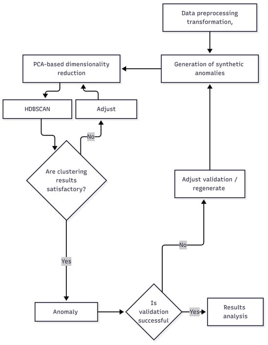
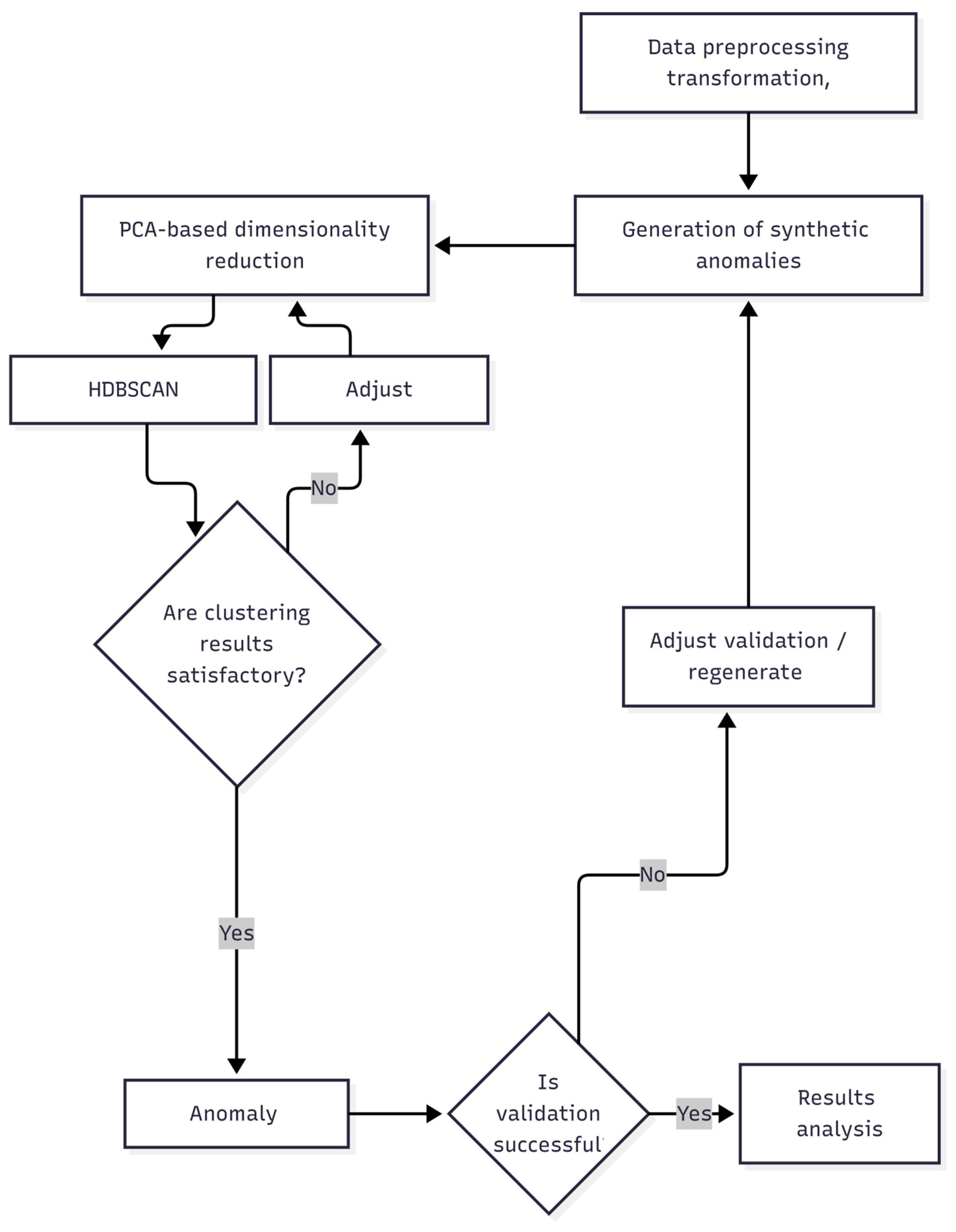
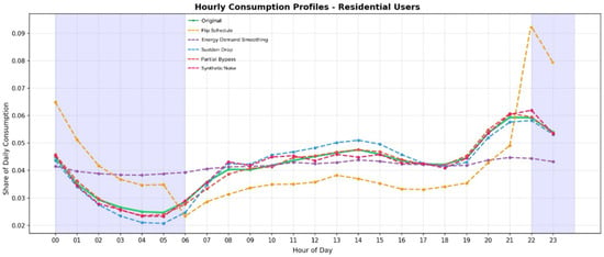
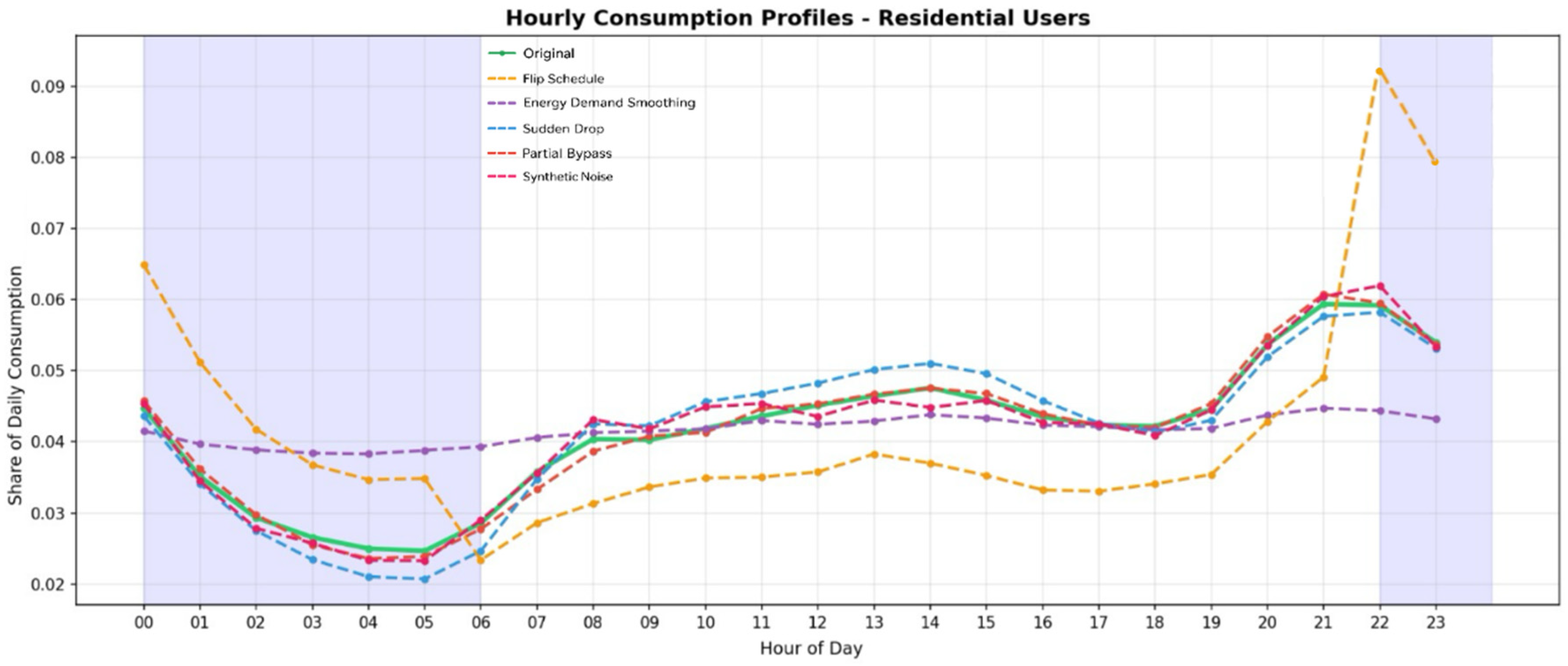
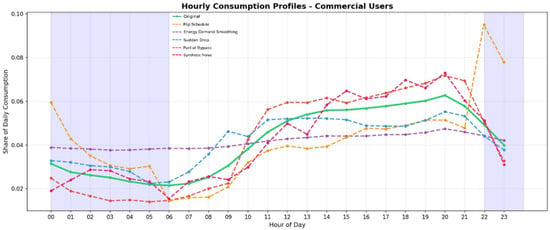
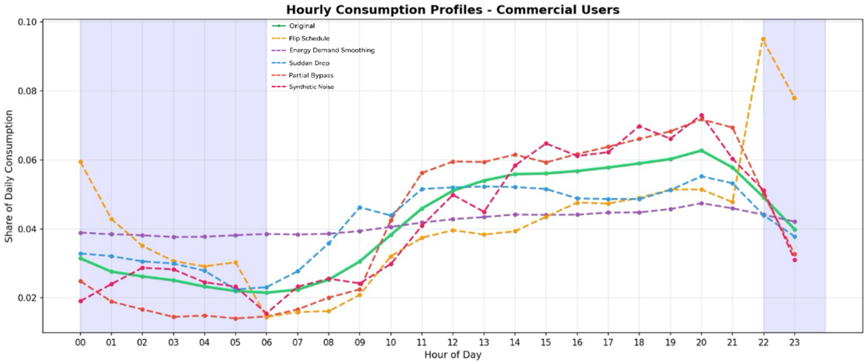
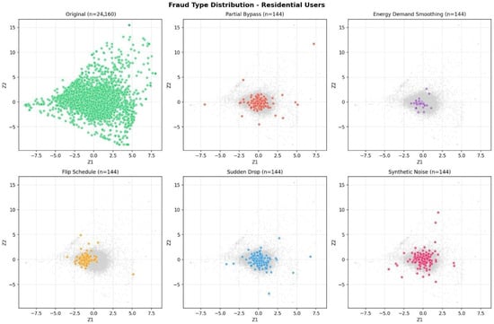
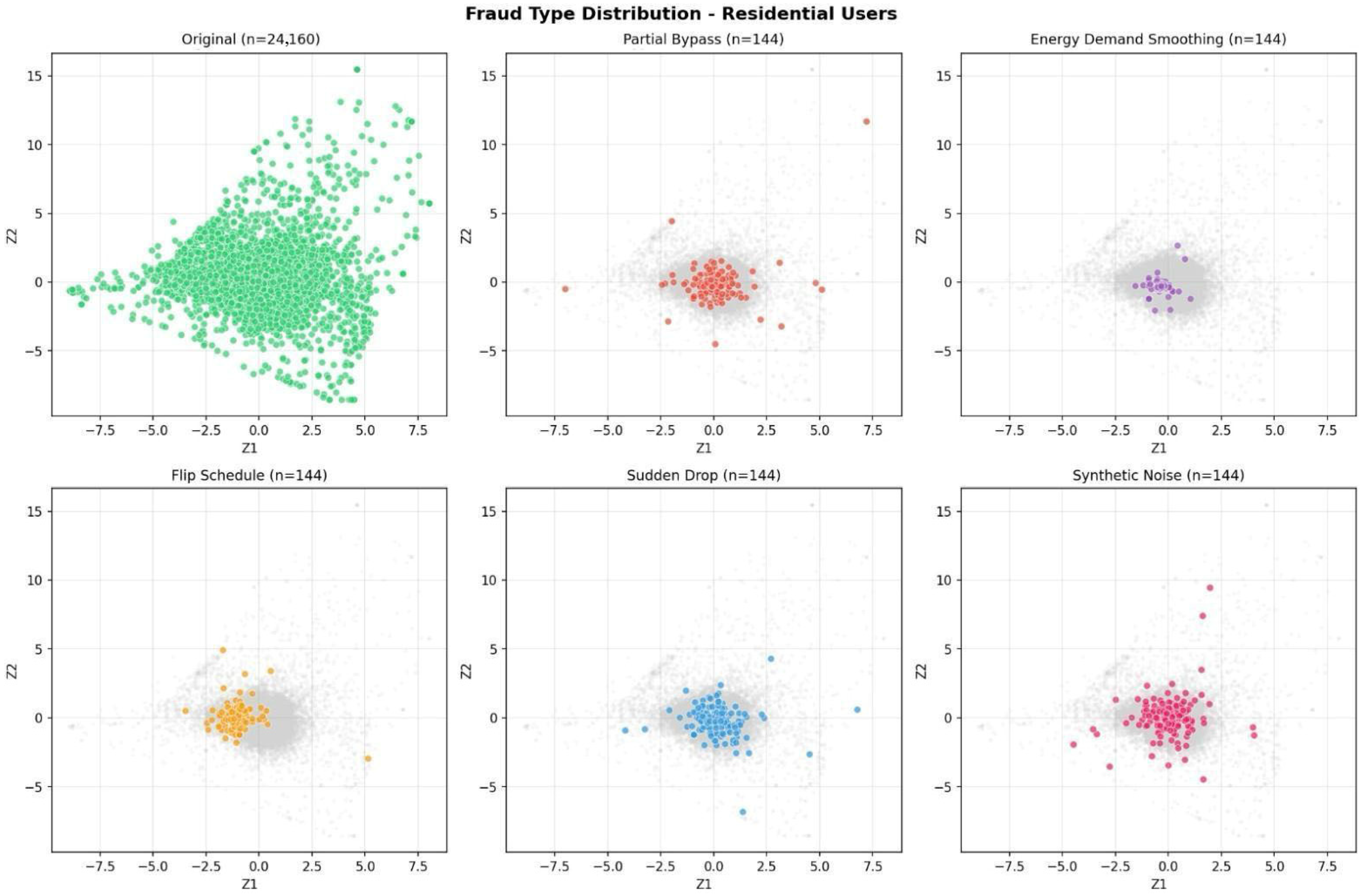
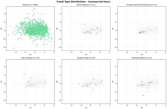
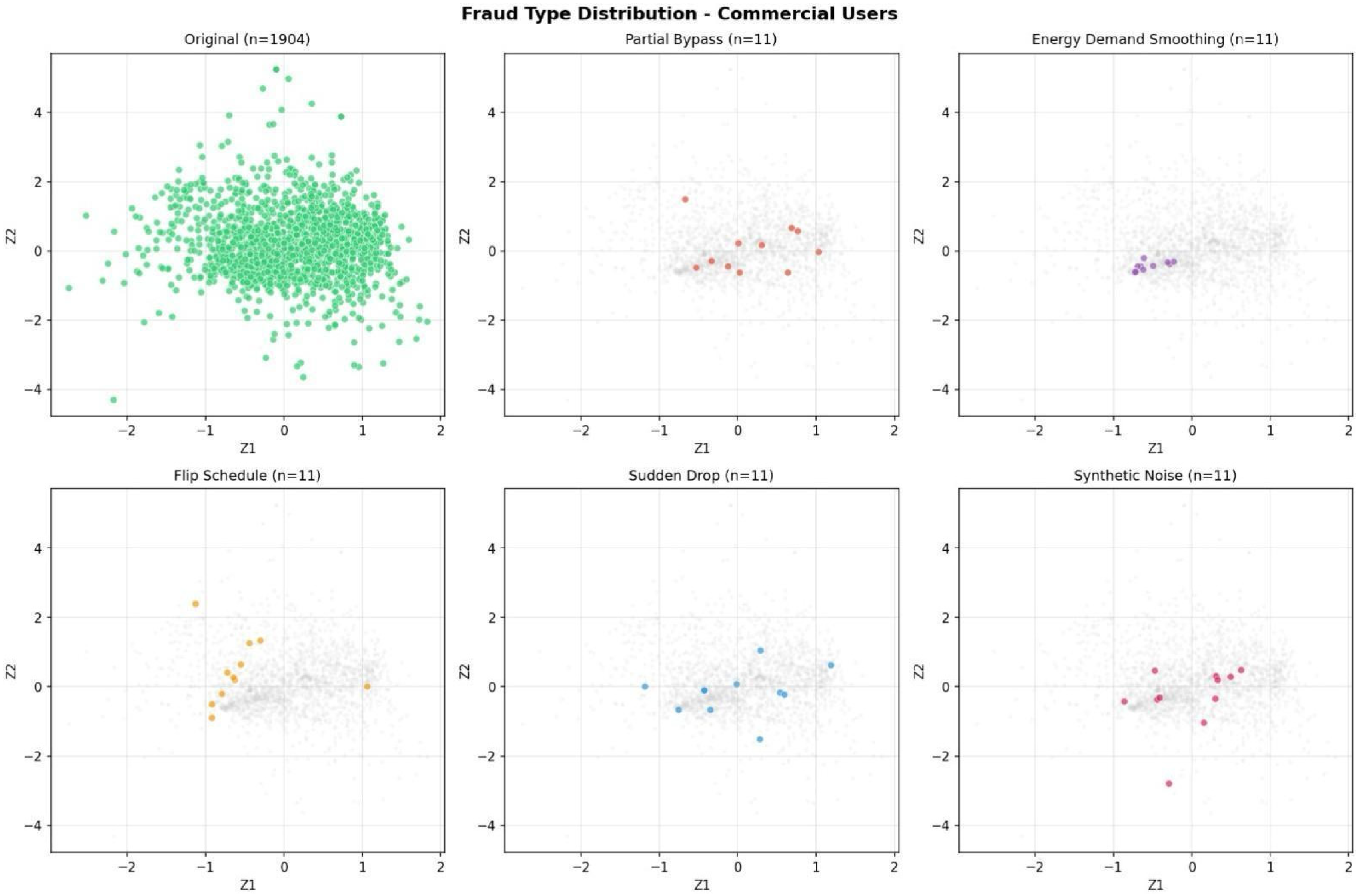
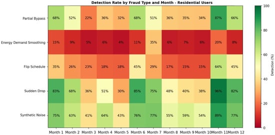
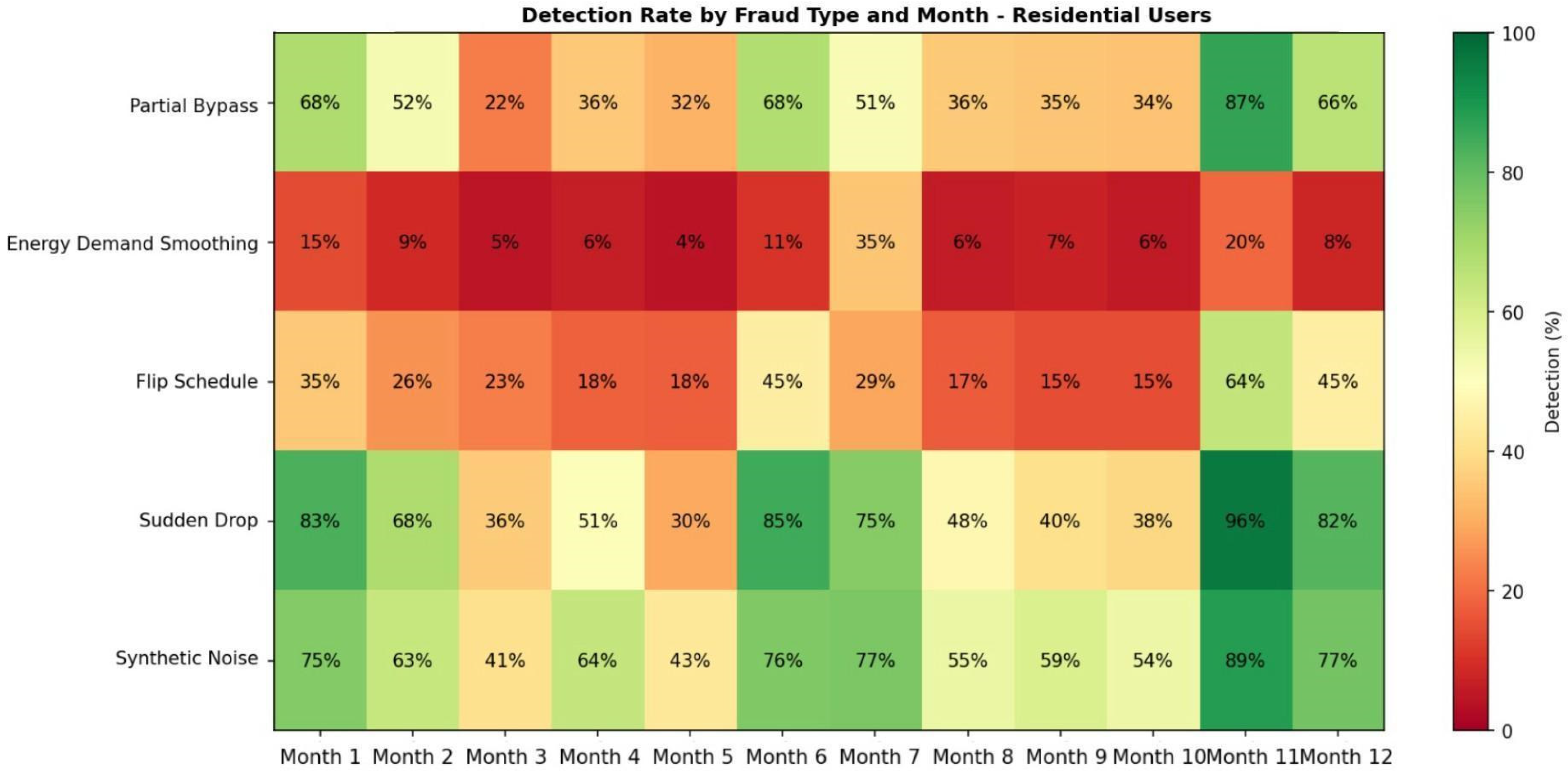
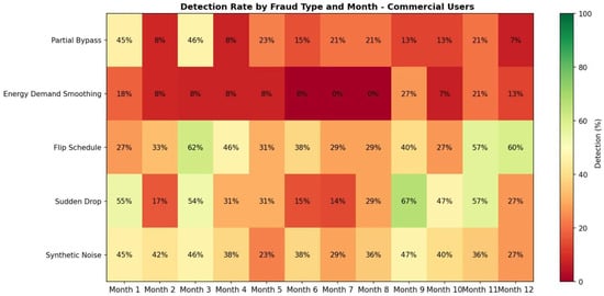
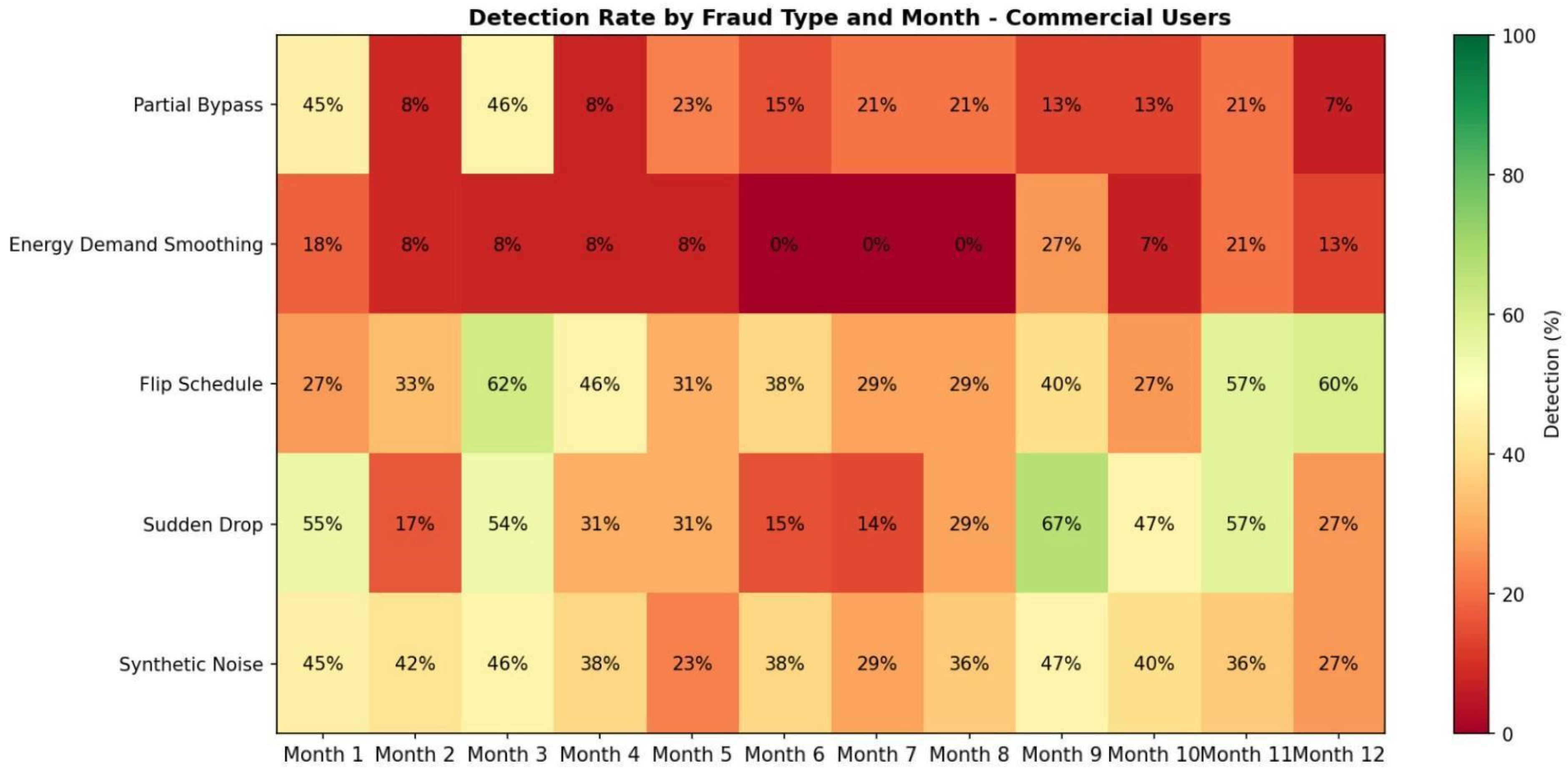

Disclaimer/Publisher’s Note: The statements, opinions and data contained in all publications are solely those of the individual author(s) and contributor(s) and not of MDPI and/or the editor(s). MDPI and/or the editor(s) disclaim responsibility for any injury to people or property resulting from any ideas, methods, instructions or products referred to in the content. |
© 2026 by the authors. Licensee MDPI, Basel, Switzerland. This article is an open access article distributed under the terms and conditions of the Creative Commons Attribution (CC BY) license.