


Abstract
The lower-velocity clay in the Yinggehai Basin (northwestern South China Sea) forms under rapid depositional conditions. These clays are typically buried at depths of 1.3–4.0 km, with P-wave velocities ranging from 2.5 to 3.0 km/s. They produce pseudo-bright spots on seismic images, often mistaken for gas sand reservoirs, thus complicating reservoir identification. When quantifying the geometric factor that characterizes the compaction state of clay using log porosity data, we found that the geometric factor calculated from the critical porosity could not effectively describe the elastic characteristics of clay. As a result, the bulk modulus was used to optimize the calculation method for the geometric factor and to improve its accuracy. A rock physics model incorporating the optimized geometric factor successfully synthesized sonic velocity curves showing higher consistency with measured acoustic logs. The refined model further elucidates the elastic and anisotropic characteristics of lower-velocity clays. Core-scale inversion of geometric factors demonstrated remarkable correlation with mineralogical composition, specifically illite and smectite content, revealing systematic alignment between geometric flattening patterns and mineralogical diagenesis. This integrated approach provides a tool for distinguishing clays from gas sand reservoirs, significantly enhancing the reliability of seismic interpretation in similar depositional environments. The findings offer critical insights for improving reservoir identification accuracy and reducing exploration risks in rapidly deposited sedimentary basins.
1. Introduction
In shallow exploration (typically at depths < 1.3 km) within the Yinggehai Basin, the seismic “bright spot” method has demonstrated high accuracy. However, in some intermediate to deep zones (approximately 1.3–4.0 km), drilling often encounters clays instead of reservoirs [1]. This discrepancy arises because the “bright spots” are generated by a set of lower-velocity clays developed within the normal clay background, forming low-impedance anomalies that appear as “seismic bright spots” on seismic profiles. These lower-velocity clays may have formed due to multiple subsidence and sedimentation episodes, leading to the accumulation of thick clay layers that, not subjected to significant compaction, retain high porosity and lower-velocity characteristics [2]. Additionally, due to rapid deposition, pore water is not expelled in the clays, leading to abnormally high pore pressures and the formation of overpressured strata.
Currently, elastic analysis of clays primarily relies on elastic experiments and rock physics modeling [3,4]. The microstructure of clays can be characterized through experimental methods such as X-ray diffraction and scanning electron microscopy (SEM) [5]. Mechanical properties are obtained through uniaxial and triaxial experiments [6]. Acoustic experiments are also widely used in the study of the elastic characteristics of clays. However, for clay samples from high-temperature and high-pressure environments, experimental costs are high, and core acquisition is challenging [7,8]. Therefore, obtaining the elastic characteristics of clays from different sedimentary stages through experiments poses significant challenges [6].
With the advancement of shale gas development and hydrocarbon source rock research, significant progress has been made in clay elastic modeling [9]. Clays typically exhibit a platy structure during compaction [10]. Thus, the corresponding rock physics is primarily based on anisotropic models [11]. For the characterization of clay minerals, anisotropic SCA (self-consistent approximation) models and DEM (differential effective medium) models are commonly used for equivalence [12,13]. The platy structure of clays forms a preferred orientation during compaction, typically exhibiting VTI (vertical transverse isotropy) anisotropy [14,15]. The anisotropy of clays is mainly described using five anisotropic parameters proposed by Thomsen, which weight the elastic characteristics in different directions [16,17]. In terms of representing the compaction state of clays, the pore structure is primarily used for description, with critical porosity being an important parameter [18]. Critical porosity refers to the porosity at which the rock skeleton structure transitions from a “particle-supported” to “suspended state” [19]. However, for rapidly deposited clays, the effectiveness of critical porosity in representing their elastic characteristics requires further verification. For example, Martín-Martín and Robles-Marín [20] discussed alternative physical calculation methods (such as the specific gravity change method and geotechnical software) for compaction assessment, suggesting that traditional porosity–depth empirical relationships may be less applicable under rapid deposition or overpressure conditions, and their applicability to rapidly deposited clays needs to be re-evaluated in similar basin settings.
This study utilizes logs to analyze the elastic characteristics of clays at different depths, explores the reliability of critical porosity in characterizing rapidly deposited clays, and optimizes the geometric factor of clay compaction state through the bulk modulus. Finally, the CMAES (Covariance Matrix Adaptation Evolution Strategy) optimization method is used to invert the geometric factor. The reliability of the geometric factor is verified through comparisons with final logs, core mineral content measurements, AVO (amplitude versus offset) attributes, and model results. The anisotropy and elastic characteristics of clays under different compaction states are further analyzed using the rock physics model based on the geometric factor. The seismic response characteristics of clays under various compaction states are obtained via forward modeling. The optimized model provides a more accurate representation of the elastic characteristics of clays in the Yinggehai Basin and establishes a new correlation between rock structure and seismic response within rapidly deposited strata. This approach offers important support and theoretical basis for future reservoir development and exploration in the region. Additionally, the research findings have significant guiding implications for characterizing the elastic characteristics of rapidly deposited clays and possess broad application value for clay studies in similar geological settings.
2. Geological Setting
The Yinggehai Basin, located at the intersection of the Indochina Block, the South China Block, and the Pacific Plate, is a large Cenozoic strike-slip-extensional basin formed by the coupling of multiple geological factors [21]. The basin has experienced multiple episodes of subsidence and sedimentation, resulting in the accumulation of thick clay-rich sequences. Tectonically, strike-slip fault activity within the basin has caused stratigraphic displacements, leading to the localized accumulation and distribution of lower-velocity clay layers [22]. Additionally, the upward migration of deep thermal fluids may have contributed to the formation and diagenesis of lower-velocity clays [23].
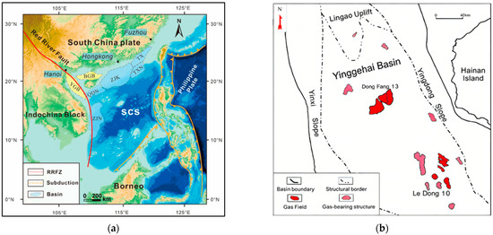
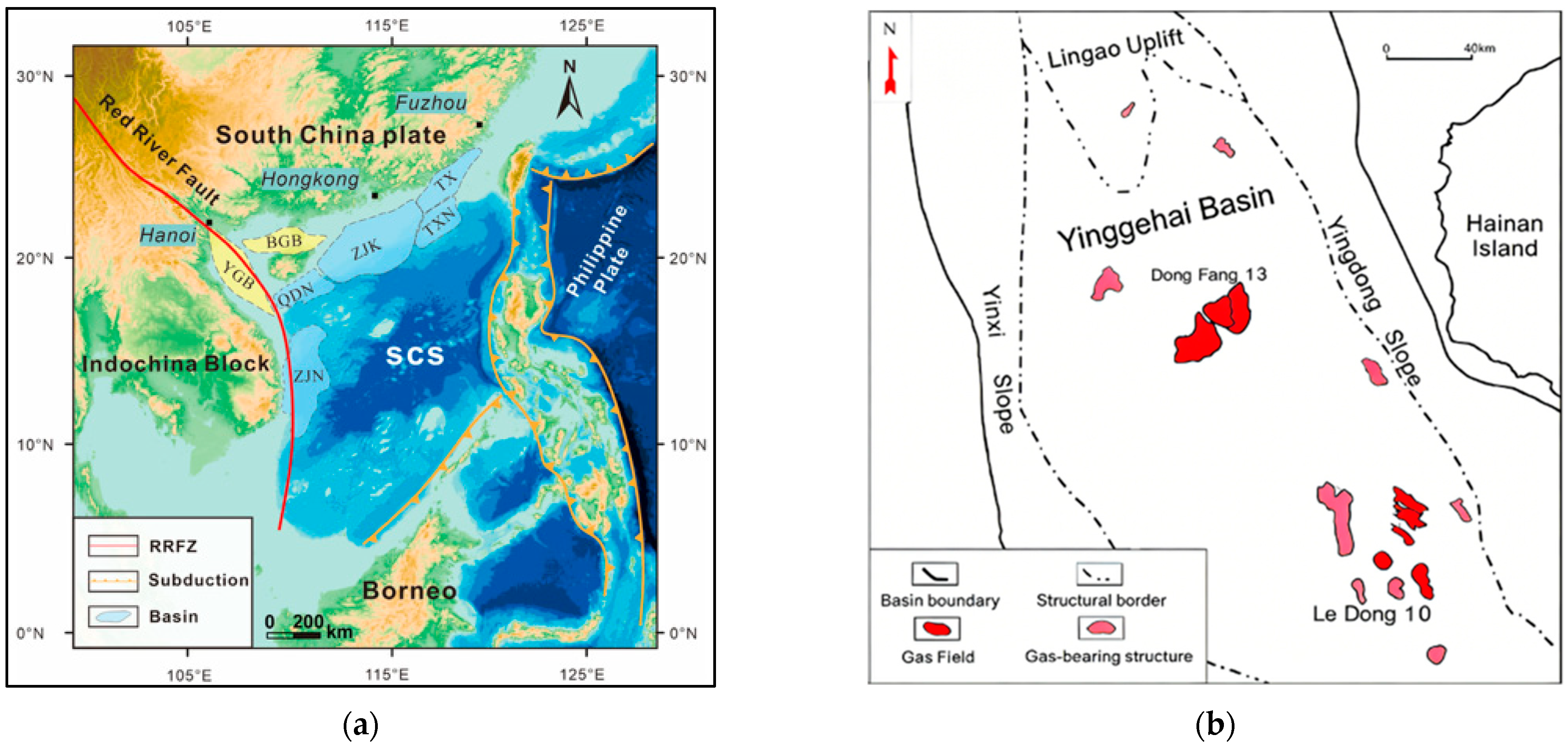
The basin is rich in natural gas resources. All data utilized in this study were obtained from the DF13 Gas Field and the LD10 Gas Field (Figure 1). These two gas fields are located in the central and eastern parts of the basin, respectively, and represent typical high-temperature and high-pressure environments. Li et al. [24] summarized the overpressure patterns of lower-velocity clay layers and analyzed the changes in clay mineral content under overpressured conditions within these fields. Therefore, analyzing the elastic characteristics of clays from different sedimentary stages is critical for the exploration of reservoirs in the Yinggehai Basin [7,25].
Figure 1.
(a) Regional location of the Yinggehai Basin (YGB). (b) Structural map of the Yinggehai Basin showing the location of the DF13 and LD10 gas fields, major structural units, and basin boundary.
3. Materials and Methods
During compaction, clay and other weak rocks develop flattened geometries. This means that the clay matrix cannot be described using the isotropic model to capture its anisotropic elastic characteristics [26]. Instead, the flat structure of clay is equivalently represented by its flatness, which is characterized by the geometric factors of the clay domain [14]. Moreover, if these flattened geometries are arranged with a preferred orientation, they will further induce elastic anisotropy. Generally, due to a dominant geological sedimentation factor, clay domains typically exhibit a preferred orientation [27].
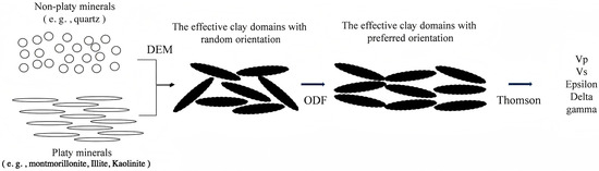
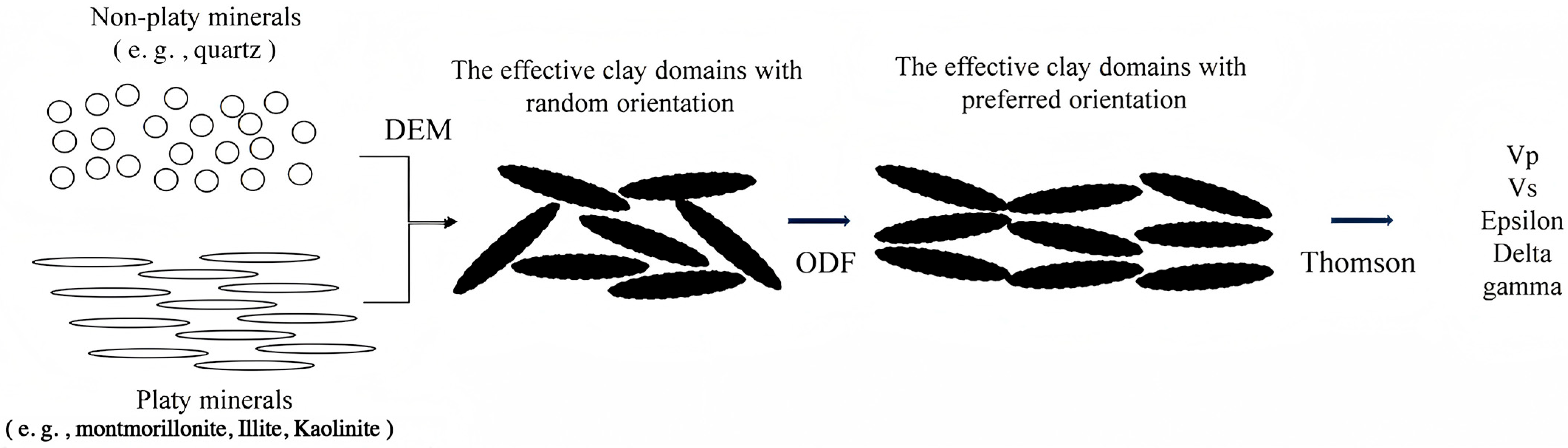
Based on the structural characteristics of clay, we constructed its corresponding rock physics model in three main steps (Figure 2) [28]. The first step involves modeling individual clay domains using the anisotropic differential effective medium (DEM) model proposed by Hornby et al. [12]. In the second step, we apply the orientation distribution function (ODF) to the weighted average of the elastic matrices of clay domains in different orientations, as described by Johansen et al. [29]. Finally, we calculate the anisotropic parameters of the clay using Thomsen’s anisotropic model [17]. For this modeling workflow, we computed the geometric factor AR—used in Steps 1 and 2 to characterize clay compaction—from the bulk modulus rather than from the critical porosity.
Figure 2.
Clay-modeling workflow: (1) construction of an equivalent-clay domain via a DEM model (random distribution), (2) orientation-weighted homogenization of the clay domain using the ODF, and (3) calculation of anisotropic elastic parameters for clay with a preferred orientation.
In this section, we describe the three-step rock physics modeling workflow for clay (DEM → ODF → anisotropic parameters) and the optimization of the geometric factor AR using the bulk modulus. The outputs of this workflow are validated against well-log data, as shown in Figure 3 (Section 3.1), Figure 4 (Section 3.3), Figure 5 and Figure 6 (Section 3.4), and Figures 8–11 (Section 4).
3.1. The Differential Effective Medium Model
This subsection presents the differential effective medium (DEM) model used to compute the effective stiffness matrix of a single clay domain with a given geometric factor AR. The DEM model involves subdividing the inclusion phase with a specific aspect ratio (geometric factor AR) into small sub-portions and incrementally inserting these sub-portions into the background phase [30,31]. Hornby et al. [12] adapted the DEM model to the equivalent single clay domain. The core equation of the modified DEM is as follows:
Here, is the factor that incorporates the aspect ratio AR of the inserted phase [32]. is the stiffness matrix of the inserted phase, and represents the total volume fraction of the sub-portions of the second phase inserted during the -th iteration. is the unit (fourth-order) tensor. is the background stiffness matrix before the -th insertion (for the first insertion, the background phase is the host medium). The equivalent stiffness matrix of each inserted sub-phase can be determined using Equation (1). The stiffness matrix after the -th insertion can be expressed as:
Through this iterative process, the effective stiffness matrix of the inserted phase with a specific aspect ratio can be obtained. In this study, the background phase consists of non-laminated minerals, while the inserted phase is composed of laminated minerals. The elastic stiffness matrix of the clay domain () can be calculated using Equations (1) and (2). The effective stiffness matrix Cclay obtained here serves as the input for the ODF upscaling in Section 3.2. The sensitivity of the DEM model to different AR values is validated in Figure 3.
Figure 3.
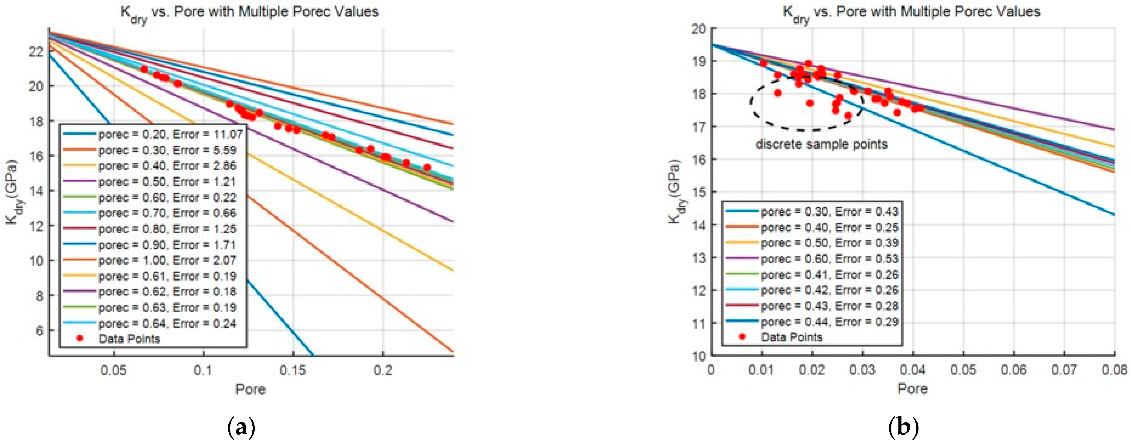
Model results for different critical porosity values: red markers denote well-log measurement samples. (a) Critical porosity model results for a normal shale interval (a critical porosity of 0.18 provides the best fit to the measurements); (b) critical porosity model results for the lower-velocity clay sample, with the points inside the black circle where the model cannot be applied.
3.2. The Orientation Distribution Function
This subsection describes the orientation distribution function (ODF) used to upscale the elastic properties from randomly oriented clay domains to a medium with a preferred orientation (VTI symmetry). Roe [33] proposed the orientation distribution function (ODF) for the spatial distribution of objects. The direction of any object with a specific orientation in space can be described by a directional function of the three angles between its own Cartesian coordinate system and the Cartesian coordinate system of the space [34]. We applied these ODFs to characterize the directional properties of the clay domains computed in Section 3.1. The ODF must satisfy the following conditions:
The directional function of the three angles can be expanded as a series of Legendre polynomials. The Legendre coefficients in the equation serve as the mathematical representation of its direction:
Sayers [35] further derived the directional function for vertically transverse isotropic (VTI) media. For VTI media, the directionality can be expressed solely by the Legendre coefficients and . He also provided the Voigt-averaged stiffness matrix for clays corresponding to these two Legendre coefficients:
Here, and are the Lamé constants of a single clay domain. , , and can be expressed by the as follows:
For the VTI-symmetry of clays, the ODF can be simplified to DDF (directional distribution function) in the horizontal plane. simplifies to . Johansen et al. [29] studied the DDF function for clay orientation with different strain aspect ratios (A) and provided the expressions for and :
Thus, via Equations (6)–(11), we compute the five independent stiffness coefficients of the elastic stiffness matrix of clay with a preferred orientation using A as the input parameter; the detailed procedure for calculating A will be presented in the next subsection. The five independent stiffness coefficients computed here are used to calculate the Thomsen anisotropic parameters in Section 3.4. The resulting elastic properties will be validated against well-log data in Section 4, using the results shown in Figures 8 and 9.
3.3. A New Representation of Geometric Factor Model
This subsection introduces a new representation of the geometric factor AR. Instead of using critical porosity (Equation (21)), we optimized AR using the bulk modulus, as the critical porosity approach fails for lower-velocity clays. For simplicity, we assumed that some clay components (e.g., smectite) can be idealized as spherical crystals in an unstressed state and become flattened under overburden pressure, while other platy minerals (e.g., micas) are considered inherently flat from deposition. We used an ellipsoid to equivalently represent the individual, deformed clay domain [14]. Therefore, we can use the reciprocal of the compaction coefficient proposed by Johansen et al. [29] to represent the geometric factor AR that describes the degree of flattening of the clay:
Initial thickness is the layer thickness in the initial state, and final thickness is the layer thickness after compaction. characterizes the degree of flattening of the clay (the larger the AR value, the closer the clay is to a spherical shape; otherwise, the smaller the AR value, the closer it is to a platy structure). We also used this AR as the aspect ratio input parameter in the DEM model.
Bachrach [36] analyzed the relationship between the compaction state of clay and its porosity. Based the critical porosity, he further simplified the formula for AR as follows:
The porec is the critical porosity. is a model parameter for compaction state. The critical porosity is the threshold at which the rock skeleton completely loses its stiffness and transitions into a particle suspension state. The critical porosity reflects the rock skeleton’s resistance to compression. Determining the critical porosity of rocks is relatively challenging. Nur et al. [19] optimized the relationship between linear modulus and porosity as follows:
where is the modulus of the rock skeleton, and is the modulus of the rock matrix.
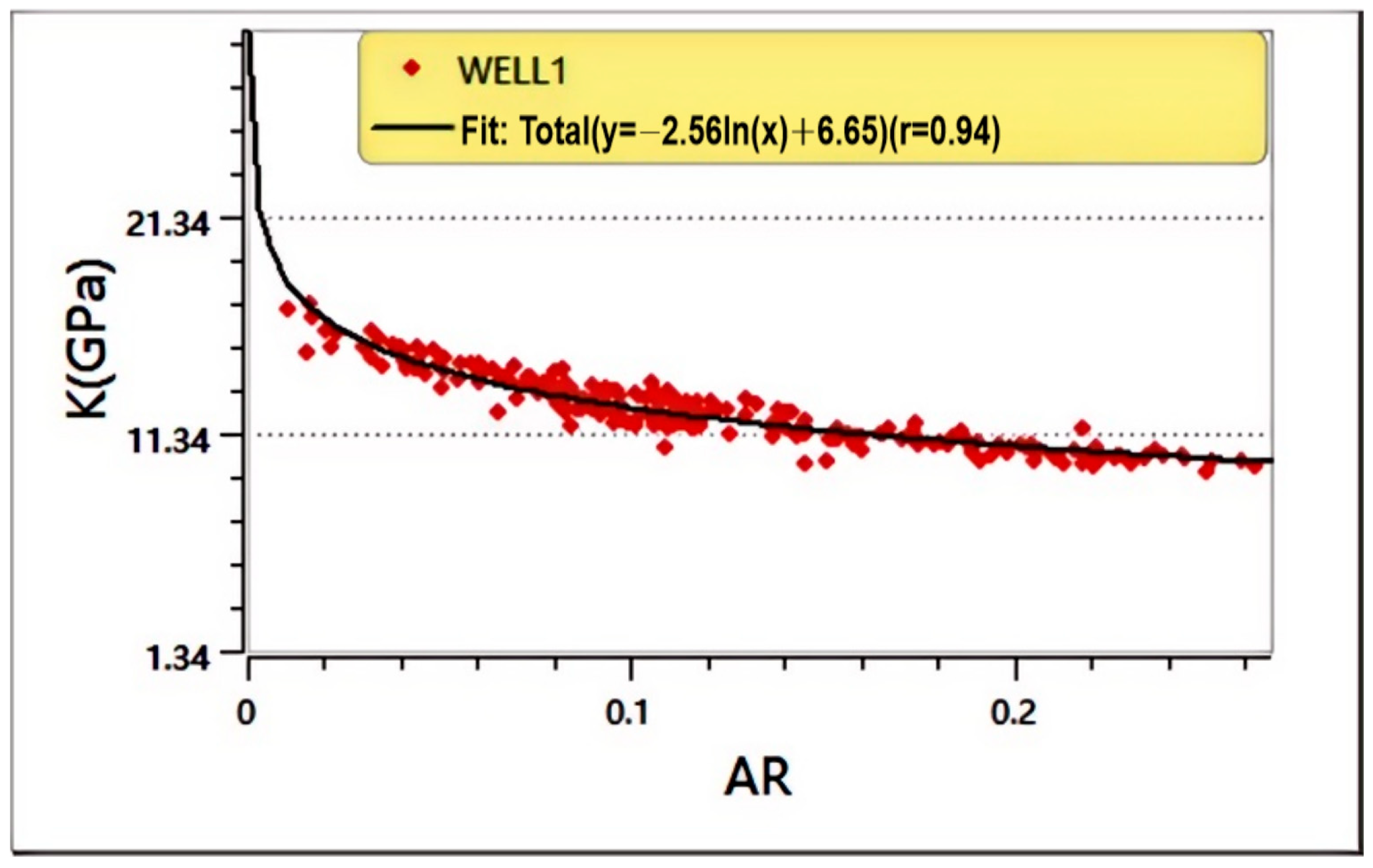
We analyzed the critical porosity model results of clay from the well-log data and compared them with the sonic logging outcomes (Figure 3). Figure 3a presents the critical porosity model results for the normally compacted clay, whereas Figure 3b illustrates those for the lower-velocity clay. Clearly, the critical porosity effectively describes the elastic properties of normally compacted clay, while significant errors arise when using the critical porosity model to represent the elastic characteristics of lower-velocity clay. This discrepancy is attributable to the heterogeneous compaction state of the clay under overpressure conditions. Therefore, the sedimentary pattern in rapid deposition sections may differ significantly from the normal compaction pattern, and the critical porosity in this section varies accordingly. Consequently, the application of Equation (21) to calculate the geometrical factor for lower-velocity clay is unfeasible. Figure 3a confirms that the calculated geometrical factor for the normally compacted clay is reliable, and we performed correlation analysis with the bulk modulus as shown in Figure 4. The geometrical factor, computed based on critical porosity, exhibited an exponential relationship with the bulk modulus, with a correlation coefficient of 0.944. Therefore, we substituted Equation (21) with a function relating the bulk modulus to the geometrical factor. The optimized geometric factor AR was used as the input for the DEM model (Section 3.1) and ODF upscaling (Section 3.2). The relationship between AR and bulk modulus is shown in Section 3.3 (Figure 4), and the failure of the critical porosity model is demonstrated in Figure 3.
Figure 4.
Cross plot of the geometrical factor and bulk modulus for normal clay. Red markers denote well-log sample points; the black curve represents the fitted line (correlation coefficient r = 0.94, indicating a strong correlation).
3.4. Impact of Geometric Factor on Thomsen Anisotropic Parameters
This subsection describes how the Thomsen anisotropic parameters (ε, γ, δ) are calculated from the stiffness matrix obtained in Section 3.2. Thomsen [17] used the longitudinal and shear waves of a VTI medium along with three anisotropic parameters to describe its anisotropy. The anisotropic parameters can be calculated from the stiffness matrix obtained in the previous step using the following equations:
where is the P-wave anisotropy parameter, which describes the relative difference in P-wave velocity between the horizontal and vertical directions. is the SH-wave anisotropy parameter, which characterizes the anisotropy of shear wave velocity polarized horizontally (SH-wave) in different azimuthal directions. is the parameter that describes the anisotropy affecting near-vertical P-wave propagation and the velocity difference between P-waves and SV-waves, and is particularly sensitive to the variations in P-wave velocity at small angles from the vertical direction. Thus, the clay stiffness computed in Section 3.2 can be transformed into anisotropic parameters using the Thomsen model.
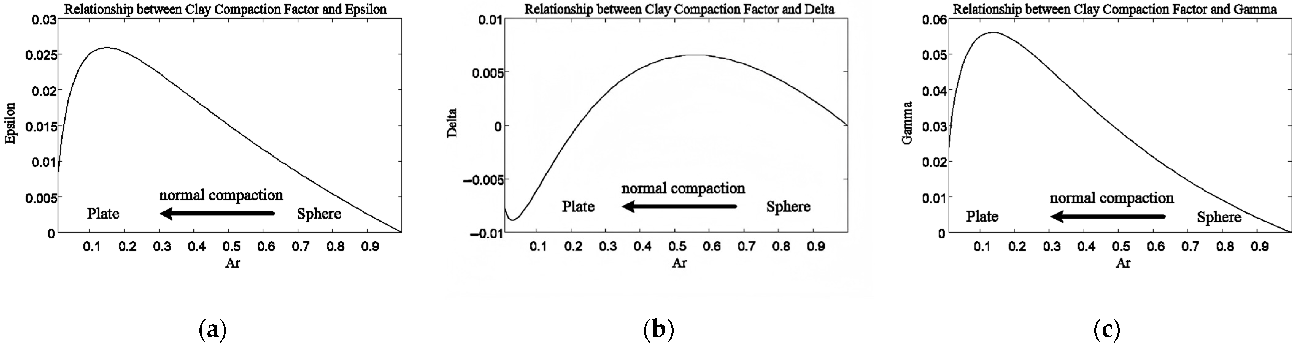
We further conducted an elastic and anisotropic analysis of the clay geometric factors using the rock physics model. As shown in Figure 5, under normal compaction, the clay deforms from a spherical to a flattened shape. The greater the degree of compaction, the flatter the clay becomes, and the smaller the geometric factor. Consequently, the clay’s P-wave and S-wave velocities increase. In addition, anisotropy increases with compaction, with both P-wave and S-wave anisotropy ( and ) increasing as compaction progresses. However, beyond an AR value of 0.13, anisotropy begins to decrease, indicating that after a certain degree of compaction, clay particle ordering weakens. The anisotropy between P-waves and S-waves (δ) does not exhibit a particularly clear trend with compaction intensity (Figure 6). The anisotropic parameters computed here are shown in Figure 5 and Figure 6.
Figure 5.
Analysis results of the geometrical-factor model based on bulk modulus. (a) Relationship between clay compaction factor () and P-wave velocity (Vp); (b) Relationship between clay compaction factor () and S-wave velocity (Vs). As compaction increases, the geometrical factor decreases, the rock becomes more flattened, and both P-wave and S-wave velocities continuously increases.
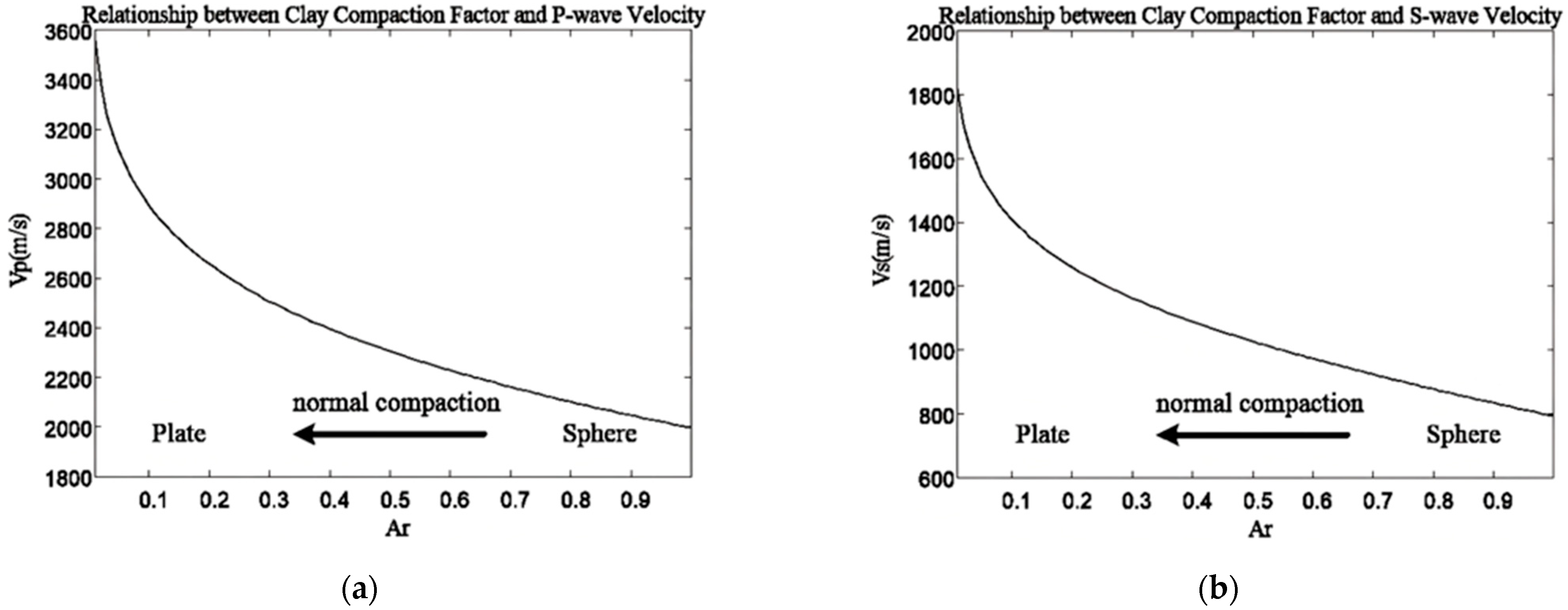
Figure 6.
Anisotropy analysis results of the geometrical-factor model based on bulk modulus. (a) Relationship between clay compaction factor and ; (b) Relationship between clay compaction factor and ; (c) Relationship between clay compaction factor and . The anisotropy patterns show that directional dependence is not determined solely by geometric morphology (nonmonotonic), but also by the orientation distribution of these geometric features.
3.5. Reservoir Modeling Workflow and Input Parameters
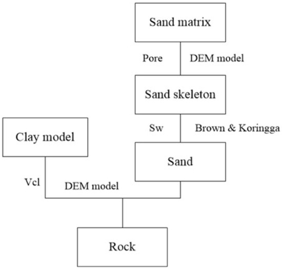
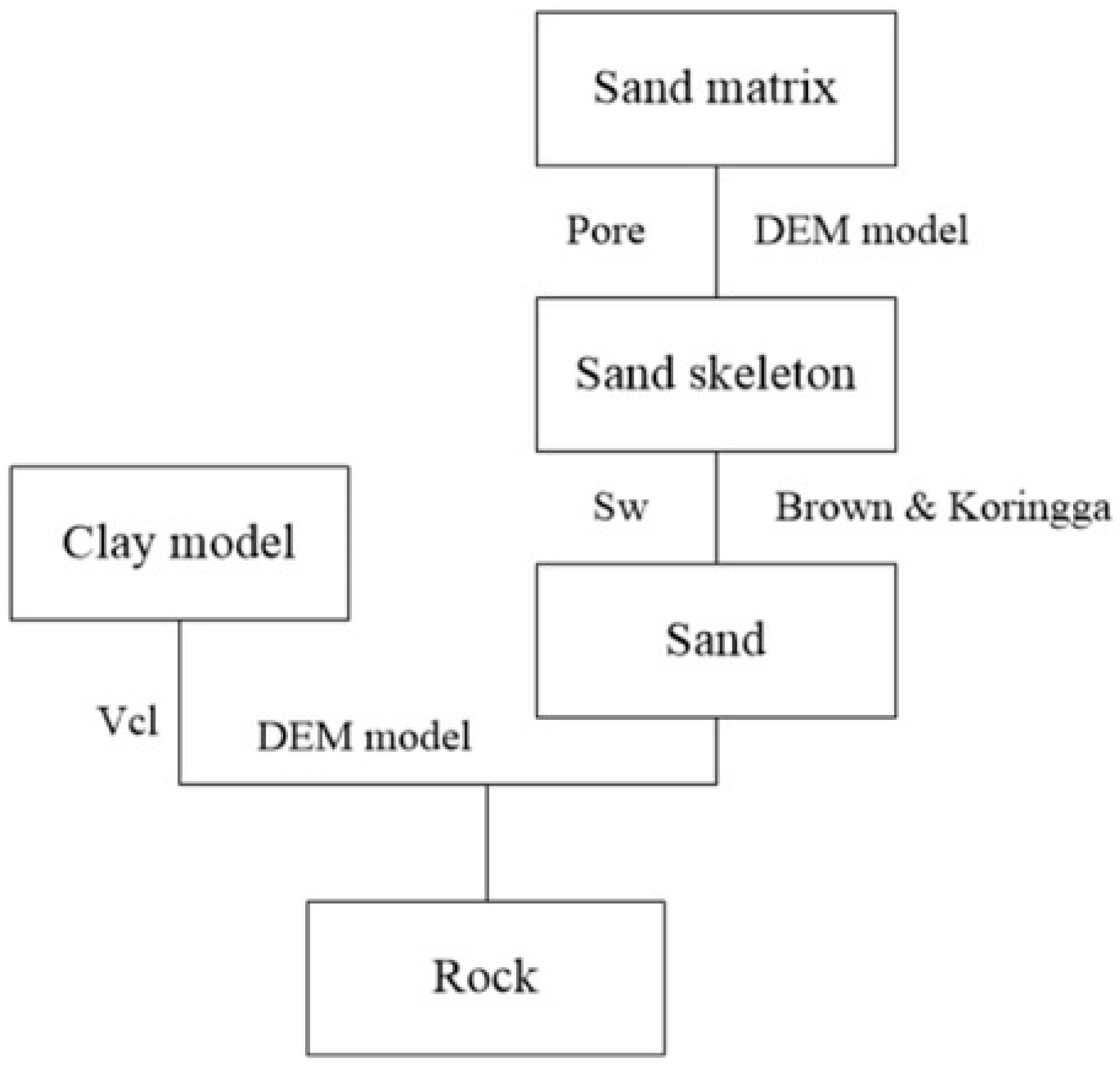
To synthesize the overall model results for validation, we supplemented the clay model with the elastic parameters of sandstone. The complete reservoir modeling workflow is illustrated in Figure 7. The primary log interpretation curves include porosity, clay content, and saturation. Background elastic parameters for minerals and fluids adopted in the modeling are listed in Table 1.
Figure 7.
Complete reservoir modeling workflow: the shale modeling sequence is detailed in Figure 2; sandstone porosity is introduced by inserting pores via a DEM model; fluids are incorporated using the BK model; and finally, the rock model is synthesized through a DEM model.
Table 1.
Table of background parameters for rock physics modeling. These data primarily originated from the Appendix in “The Rock Physics Handbook” [37] and represent the most commonly used fundamental rock parameters in the field.
4. Results
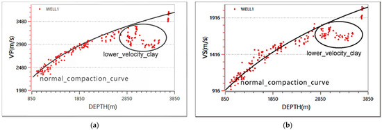
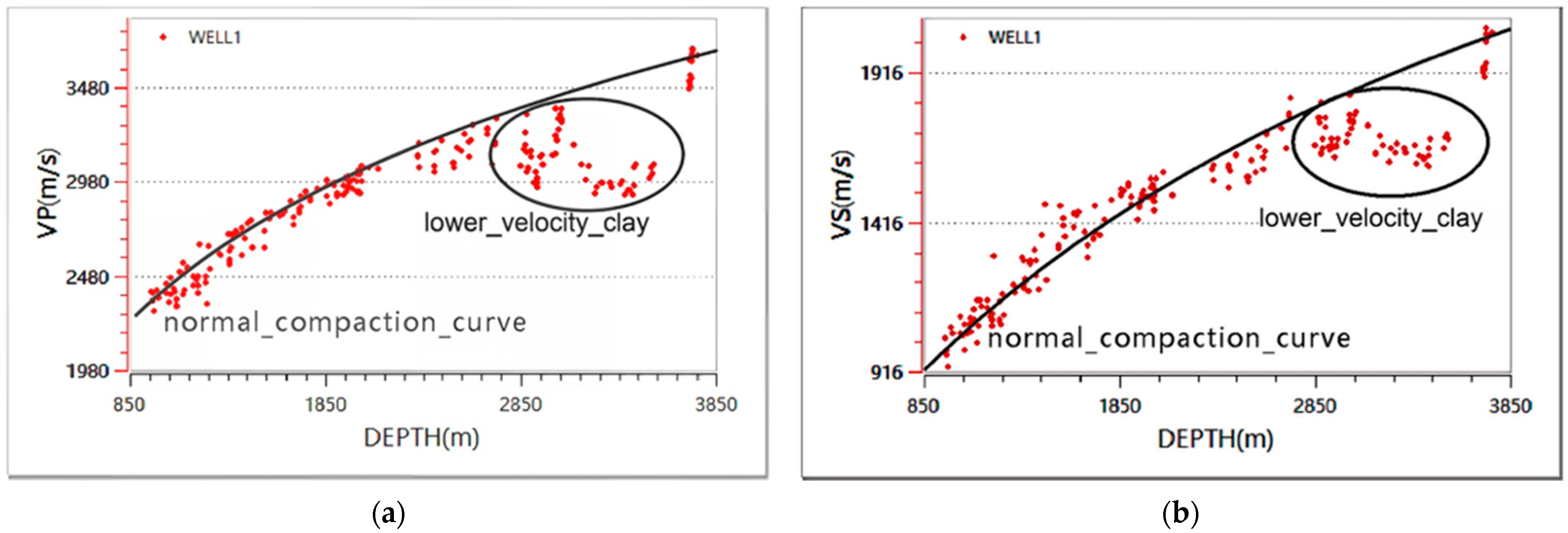
The normal compaction trend (NCT) is defined as the systematic decrease in porosity and increase in velocity with depth under conditions of steady burial, effective drainage, and hydrostatic pore pressure [38,39]. In this study, the NCT was established from well-log data in normally compacted intervals. Following the exponential porosity–depth relationship proposed by Athy [38] and later extended to velocity–depth relations by Magara [39], the NCT can be expressed as V(z) = V0e−bz. Deviations from this NCT—where measured velocities are significantly lower than the trend—indicate undercompaction or overpressure, defining the lower-velocity clay studied in this work.
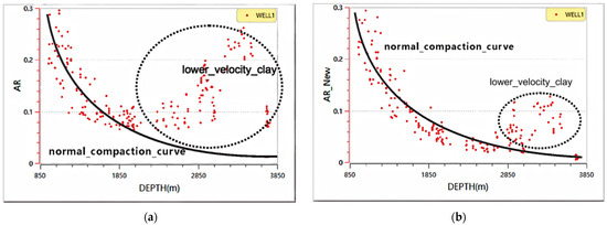
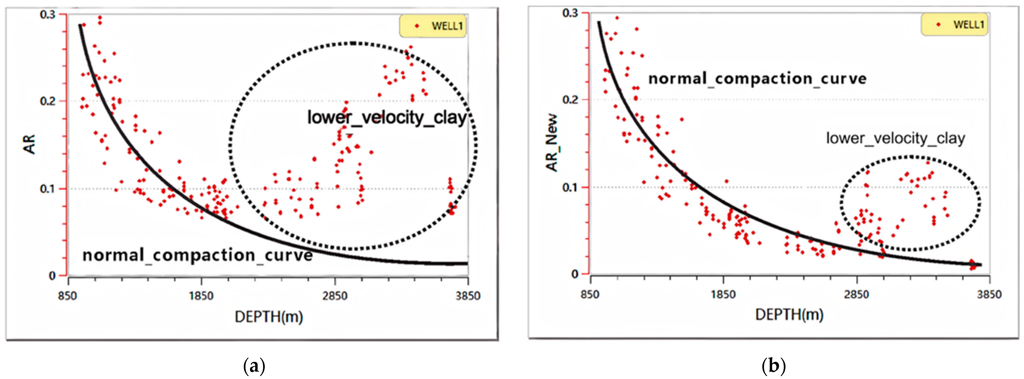
We extracted the P-wave and S-wave velocities from the sonic log in the clay section (Figure 8). The circle in the figure indicates the rapid deposition zone of the Yinggehai Basin. In this area, overpressure reduces the effective stress acting on the clay framework, leading to incomplete compaction. Consequently, the velocity of the clay deviates from the normal compaction trend, and such deposits are defined as lower-velocity clay. We calculated the distribution of the geometric factor (Figure 9). Although the two calculation methods yielded different values of the geometric factor within the rapid-deposition interval, they displayed the same trend: the geometric factor begins to increase in this interval. This indicates that the compaction degree of the clay in the rapid deposition section is lower than that in the adjacent upper sections, which are normally compacted.
Figure 8.
Variation of shale velocity with depth: red scatter points represent well-log measurements; the black line denotes the normal compaction trend; sample points within the black circle indicate lower-velocity shale. (a) P-wave velocity (VP) variation with depth; (b) S-wave velocity (VS) variation with depth.
Figure 9.
Geometrical factor results at various depths computed by two methods: red markers denote well-log sample points; the black curve shows the normal compaction trend. (a) Results based on the critical porosity model; (b) Results based on the bulk modulus model.
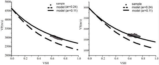
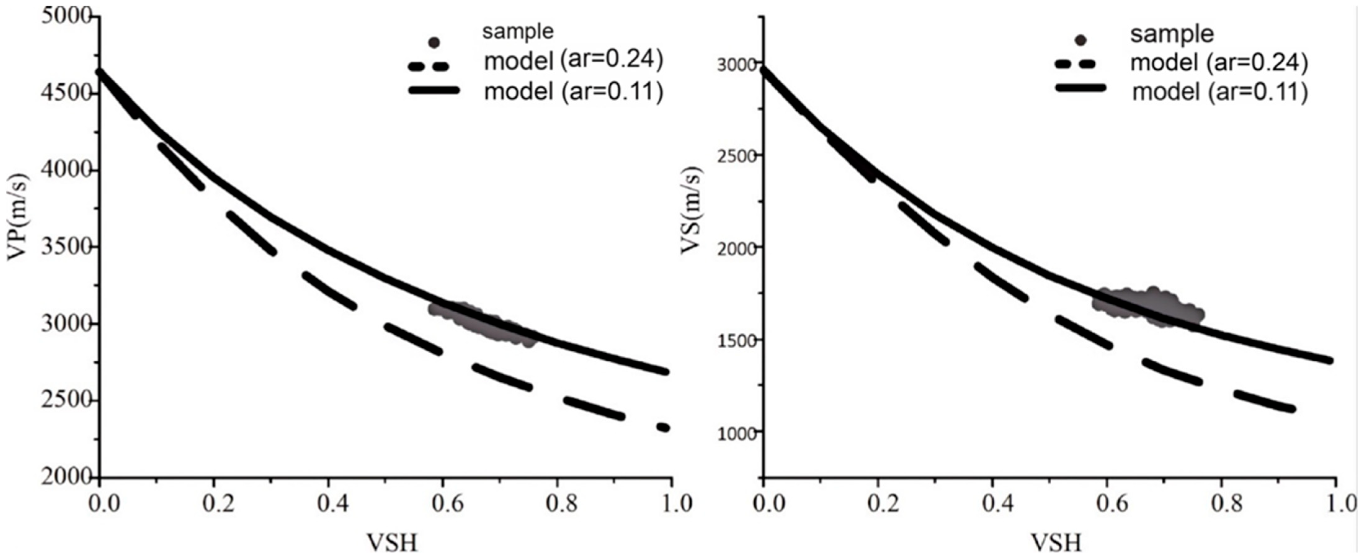
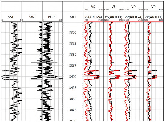
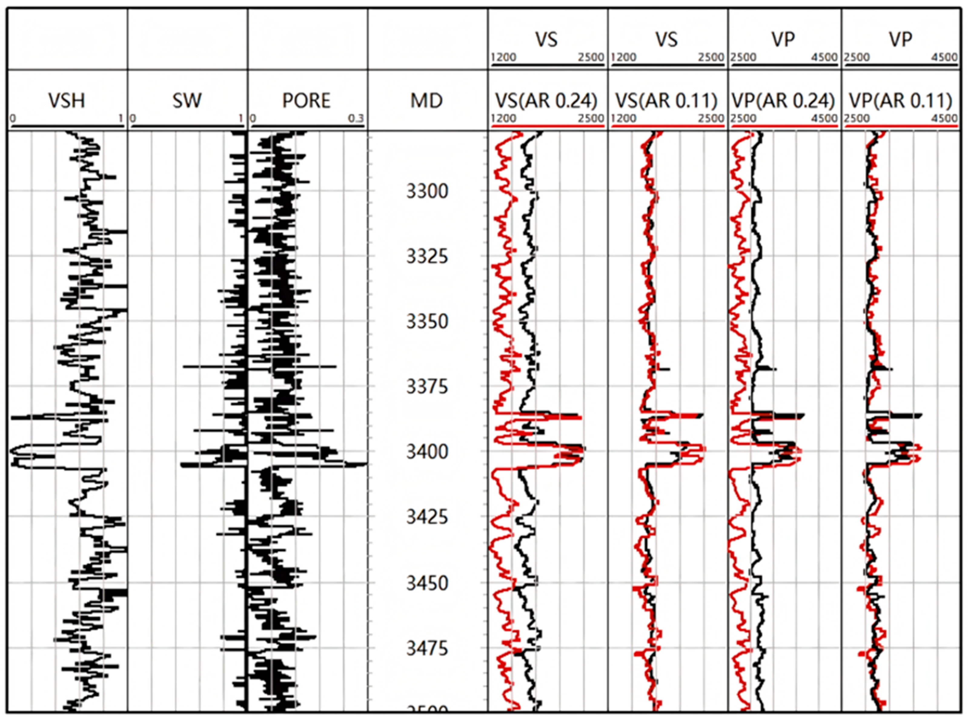
To further assess the reliability of the optimized clay modeling workflow, we validated it using the sonic curve from the lower-velocity mudstone depth interval. The geometrical factor calculated based on the critical porosity was set to 0.24, while that corrected by the bulk modulus was set to 0.11. The final model results are shown in Figure 10 and Figure 11. The corrected geometrical factor better represented the elastic velocity of the lower-velocity mudstone interval, whereas the clay velocity computed using the critical porosity was lower than the measured velocity. Hence, it is necessary to revise the computation of the geometrical factor using the bulk modulus.
Figure 10.
Comparison of geometrical factor and measurements for the lower velocity shale sample: shale sample points and model trends (gray markers are the samples; the dashed line is the critical-porosity model with AR = 0.24; the solid line is the bulk-modulus model with AR = 0.11).
Figure 11.
Comparison of geometrical factor and measurements for the low velocity shale sample: comparison of the two models synthetic acoustic curves (red) against the measured curve (black).
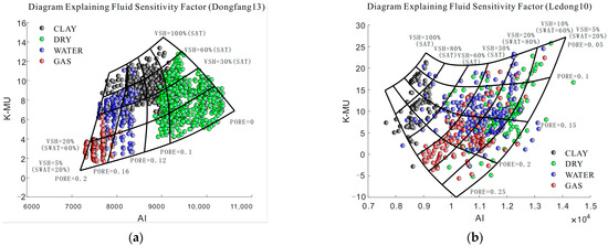
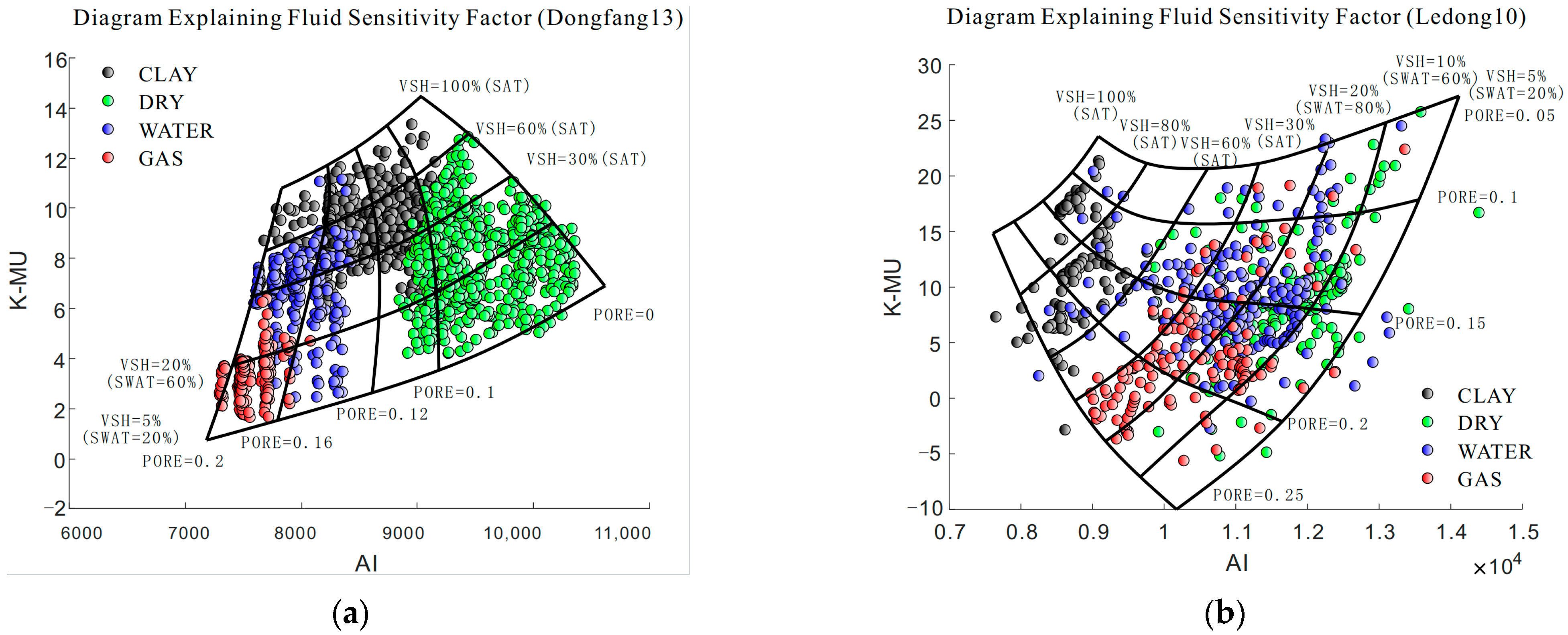
Clay anisotropy is primarily caused by two factors: the plate-like geometric shape and the preferred orientation of the plates [29]. The anisotropic changes in clay dimensions under compaction are nonlinear. Li et al. [24] observed that the alignment of clay minerals in the Yinggehai Basin is not a simple, uniform change. Due to the elastic characteristics of lower-velocity clay, which are insensitive to the changes in the AR value between P-wave and S-wave velocities, and because shear waves do not propagate through the fluids in the reservoir but only influence the P-wave behavior, we constructed a petrophysical interpretation model using the difference between the bulk modulus and the shear modulus. This helps in identifying reservoirs in the Yinggehai Basin. As shown in Figure 12, the difference between the bulk modulus and shear modulus effectively filters out gas-bearing reservoirs.
Figure 12.
Interpretation chart based on rock physics model of the Yinggehai Basin. (a) Fluid sensitivity factor diagram for the Dongfang 13 block; (b) Fluid sensitivity factor diagram for the Ledong 10 block. The green dots represent dry rock samples, black dots indicate shale samples, blue dots correspond to water-saturation samples, and red dots denote gas-saturation samples. The curve represents the results calculated from the rock physics model.
4.1. Forward Modeling Results
After verifying the reliability of the model, we further conducted prestack forward modeling of the elastic parameters for the reservoir and lower-velocity clay to assess their geophysical responses, and validated the results using AVO data collected by Liu et al. [1]. In addition, we compared the inversion results derived from the model with mineral interpretation outcomes from the acquired diffraction data, further discussing the relationship between the geometrical factor and lithology.
Furthermore, to analyze the characteristics of lower-velocity clay and reservoirs in the Yinggehai Basin, we statistically examined the petrophysical properties of formation reservoirs in the LD10 and DF13 areas (Table 2). Based on these geological parameters, we calculated the elastic properties of the lower-velocity clay, background clay, and the two gas reservoir sands (Table 3).
Table 2.
Theoretical model parameters for lower-velocity shale and reservoirs: background is normal shale, DF13 is the lower-velocity reservoir, and LD10 is the higher-velocity reservoir.
Table 3.
Elastic property calculations from the rock physics models: computed using the workflow in Figure 9.
We obtained the reflection coefficients for different incidence angles using the Ruger approximation formula. In this study, we applied the Ruger approximation formula to calculate the reflection coefficients for clay [40,41].
where denotes the phase angle, is the vertical P-wave impedance, and is the vertical shear modulus. Subscripts 1 and 2 refer to the media above and below the reflector, respectively. and are the Thomsen anisotropy parameters. The seismic response at different angles is then synthesized through convolution with seismic wavelets (Figure 13) [42,43].
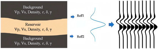
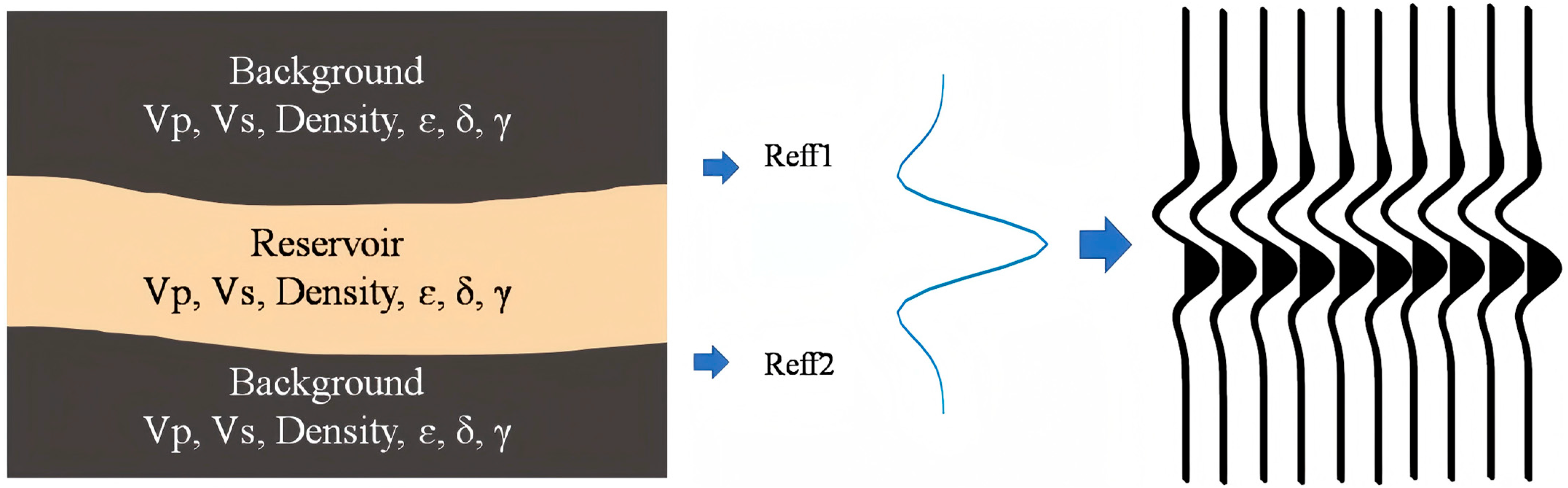
Figure 13.
Schematic diagram of the mechanism model and convolution process: The mechanism model comprises three theoretical stratigraphic layers; layer parameters are provided in Table 2. The reflection coefficients were calculated using Ruger’s approximation formula.
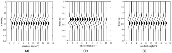
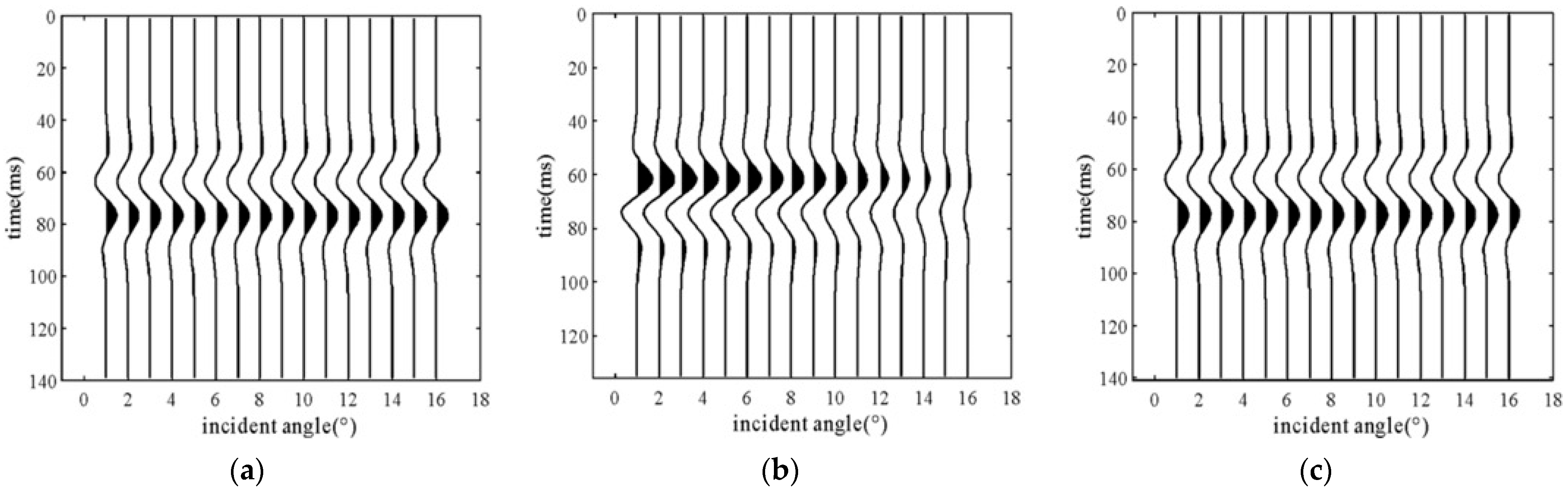
In the equation, w(t) represents the signal wavelet, and represents the reflection coefficient, corresponding to from the previous step. The is time, and the symbol denotes the convolution operation. The forward modeling results of the elastic parameters from Table 3 are shown in Figure 14. In Figure 14b, the high-velocity reservoir in Ledong shows a clear distinction from the lower-velocity clay (Figure 14c). However, the forward seismic response of the Dongfang Reservoir (Figure 14a) is difficult to distinguish from the lower-velocity clay just by examining the waveform response.
Figure 14.
Seismic responses at different incidence angles for reservoirs and lower-velocity shale: (a) response of lower-velocity reservoir in Dongfang area, (b) response of higher-velocity reservoir in Ledong area, (c) response of lower-velocity shale.
Furthermore, we fit the simplified formula proposed by Sheriff and Geldart [43] to extract the AVO intercept and gradient attributes. In addition, abundant prestack seismic AVO response attributes in this basin are available (Table 4) [1].
Table 4.
AVO classification results of lower-velocity mudstone and two types of reservoirs in Yinggehai Basin.
4.2. CMAES Inversion and XRD Analysis
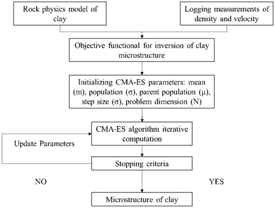
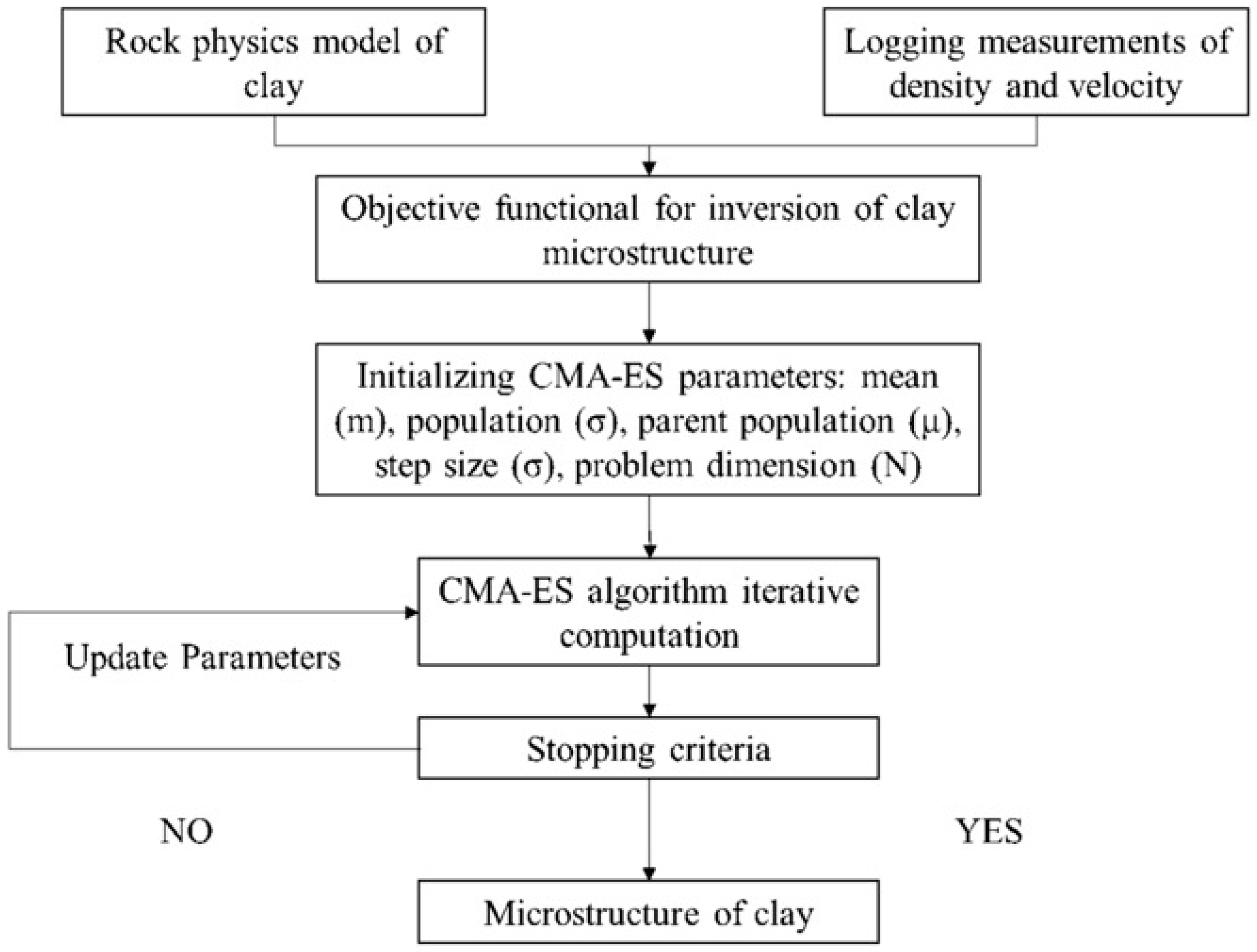
To further validate the reliability of the geometric factor, we conducted XRD diffraction measurements on core samples from the rapid deposition section. Using the CMAES (Covariance Matrix Adaptation Evolution Strategy) optimization method based on the modeling workflow in Figure 15, we inverted the geometric factor for the corresponding depth of the core samples.
Figure 15.
Geometrical factor inversion results based on CMAES: The shale modeling process is shown in Figure 2.
CMAES is an algorithm designed to solve continuous optimization problems [15,44,45]. Inspired by the process of biological evolution, this algorithm adaptively adjusts the covariance matrix to fit the characteristics of the current search space. Compared to other evolutionary algorithms, CMAES provides a flexible and powerful solution for optimizing nonlinear problems.
The main idea of the CMAES algorithm is to adjust parameters so that the probability of generating good solutions gradually increases, enhancing the likelihood of searching along the optimal solution’s direction. The computational steps of the CMAES are as follows: (1) First Stage: Generates initial sample points. (2) Second Stage: Expands the search range and the distribution range of sample points. (3) Third Stage: Updates the search range by refining the position of the optimal sample within the population, reducing the distribution space of the samples. (4) Fourth Stage: Iteratively performs the second and third stages until the output condition is met and the optimal solution is provided.
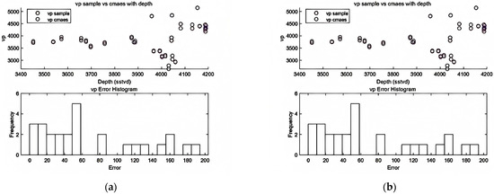
The geometric factors computed using CMAES and the corresponding errors in the well elastic parameters are shown in Figure 16.
Figure 16.
Comparison between CMA-ES inversion results and acoustic well-log measurements. Symbols represent acoustic well-log data points; open circles denote CMA-ES results (see legend for details). (a) scatter plot and error histogram for Dataset A; (b) scatter plot and error histogram for Dataset B.
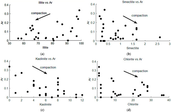
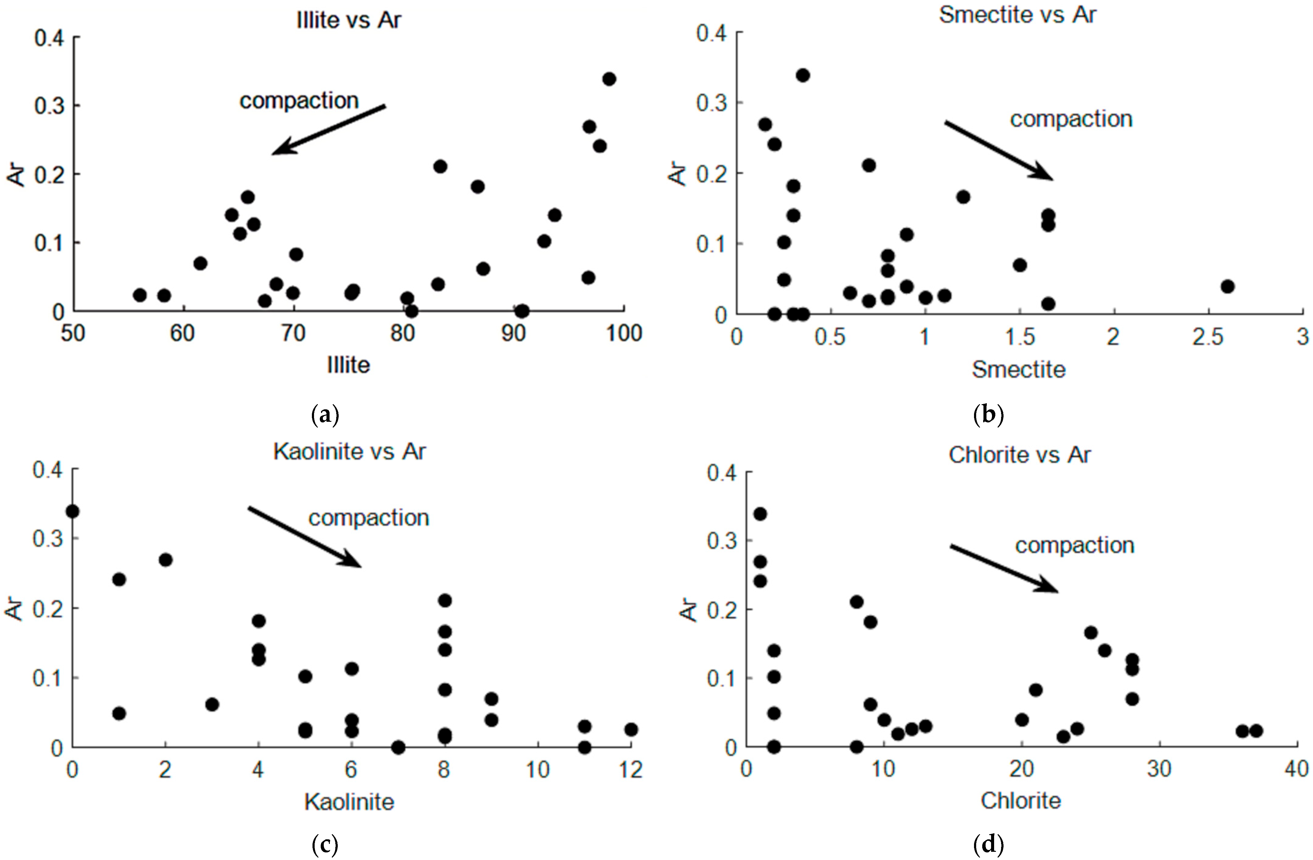
We conducted a correlation analysis between the geometrical factor and the mineral composition of clay measured by XRD (Figure 17). Based on the variation pattern of values, we identified the direction of mineral changes during clay compaction. During the compaction process, montmorillonite dehydrates and incorporates , forming illite–smectite (I/S) mixed minerals that progressively transform into pure illite [46]. In magnesium-rich environments, montmorillonite may combine with to form chlorite [47]. Kaolinite typically reacts with potassium feldspar in potassium-rich alkaline environments (e.g., ) [48]. In Figure 17, illite, chlorite, and montmorillonite all showed regular variations along the compaction trend.
Figure 17.
Comparison between CMA ES–inverted geometric factor () and core XRD mineral composition. (a) vs. Illite content; (b) vs. Smectite content; (c) vs. kaolinite content; (d) vs. Chlorite content. increases with increasing illite content, whereas it decreases with increasing kaolinite, chlorite, and smectite contents along the compaction trend.
5. Discussion
This study presents an optimized geometrical factor (AR) for characterizing clay compaction in rapid sedimentation zones, using the bulk modulus instead of critical porosity. Several key findings emerged from our results: (1) the critical-porosity model fails for lower-velocity clays in overpressure environments (Figure 3); (2) the bulk-modulus-based AR shows a strong exponential correlation with velocity (Figure 4); (3) the optimized AR improves sonic velocity prediction (Figure 10 and Figure 11); (4) AR correlates with clay mineral composition (Figure 17); and (5) AVO analysis can distinguish lower-velocity clays from gas reservoirs (Table 4, Figure 14).
5.1. Deviation from the Normal Compaction Trend
The deviation from the normal compaction trend (NCT) observed in Figure 8 is a direct consequence of rapid sedimentation and overpressure development in the Yinggehai Basin. Under normal hydrostatic conditions, clay velocity increases exponentially with depth following the Athy [38] relationship. However, in the rapid deposition zone (1.3–4.0 km), pore fluids cannot be effectively expelled, reducing effective stress and inhibiting mechanical compaction. This results in lower velocities and higher AR values (Figure 9), indicating a less flattened clay geometry. Interestingly, both the critical-porosity and bulk-modulus methods captured the same increasing trend in AR within the overpressure interval, but their absolute values differed significantly (Figure 9a,b). This suggests that while both methods detect undercompaction, the bulk-modulus method provides more accurate absolute values, as validated by sonic log matching (Figure 10).
5.2. Advantages of the Bulk-Modulus-Based Geometric Factor
The failure of the critical-porosity model for lower-velocity clays (Figure 3b) can be explained by the fact that critical porosity assumes a stable grain-contact framework that is valid under normal compaction but breaks down in undercompacted, overpressure conditions [36]. In contrast, the bulk modulus is directly sensitive to effective stress and pore pressure, making it a more robust descriptor of compaction state in non-equilibrium settings. Our results show that the bulk-modulus-based AR (0.11) yielded synthetic sonic curves that closely matched the measured logs (Figure 11), whereas the critical-porosity-based AR (0.24) underestimated velocity. This improvement is particularly significant for the Yinggehai Basin, where high temperature and high pressure (HTHP) conditions make conventional models unreliable. The exponential relationship between AR and bulk modulus (r = 0.94, Figure 4) provides a simple yet effective empirical basis for the optimization.
5.3. Non-Monotonic Relationship Between AR and Anisotropy
The non-monotonic relationship between AR and anisotropy (Figure 6) reveals that anisotropy is not solely controlled by grain shape. As compaction increases, clay platelets become increasingly aligned, initially increasing anisotropy (ε and γ). However, beyond AR = 0.13, anisotropy begins to decrease, suggesting that the orientation distribution of clay domains—rather than their individual flattening—becomes the dominant factor. This is consistent with Johansen et al. [29], who noted that the directional distribution function (DDF) plays a critical role at high compaction stages. The parameter δ does not show a clear trend with AR, indicating that near-vertical P-wave anisotropy is influenced by additional factors such as microcracks or fluid distribution.
5.4. Relationship Between AR and Clay Mineral Composition
The correlation between AR and clay mineral composition (Figure 17) provides petrological validation of our geometric factor. As shown in Figure 17, illite, chlorite, and montmorillonite follow the compaction trend (decreasing AR with increasing content), which is consistent with established diagenetic pathways [46,47,48]. The decrease in kaolinite with compaction may be due to the short burial time in the rapid deposition section (not reaching reaction equilibrium). This observation is consistent with Bjørlykke [48], who noted that kaolinite-to-illite transformation requires sufficient thermal exposure time.
5.5. AVO Classification and Reservoir Identification
The forward modeling results (Figure 14) demonstrate that the Dongfang Reservoir (DF13) and lower-velocity clay produce similar waveform responses, making them difficult to distinguish on post-stack seismic data. However, AVO analysis can effectively distinguish between the two types. The AVO classification results (Table 4) show that lower-velocity clay exhibits Class IV behavior (negative P, positive G), while the DF13 reservoir shows Class III (negative P, negative G), and the LD10 reservoir shows Class I (positive P, negative G). The consistency between our model results and the field data from Liu et al. [1] (Table 4) validates the reliability of our rock physics workflow. This indicates that AVO attributes are essential for reducing the exploration risk in the Yinggehai Basin, where pseudo-bright spots caused by lower-velocity clays are common.
5.6. Limitations and Future Work
Several limitations should be acknowledged. First, our study was based on data from a single basin (Yinggehai); further validation in other overpressure basins (e.g., Gulf of Mexico, Niger Delta) is needed to establish generalizability. Some errors may arise from the fixed values of the sandstone parameters provided in Table 1. Second, the mechanistic relationship between AR and bulk modulus requires more rigorous theoretical derivation. Our team is currently working on this aspect, and a dedicated paper focusing on the theoretical foundation is in preparation. Third, the CMAES inversion results (Figure 16) showed some errors that may be improved with better input constraints. To fully and accurately constrain all model parameters, further optimization of the model input parameters in combination with digital core technologies is necessary.
5.7. Summary of Contributions
In summary, this study provides a practical and validated solution for distinguishing lower-velocity clays from gas reservoirs in rapid sedimentation basins. The bulk-modulus-based geometric factor offers a significant improvement over conventional critical-porosity methods, with direct applications in seismic interpretation and exploration risk reduction. The integration of rock physics modeling, CMAES inversion, and AVO analysis establishes a comprehensive workflow that can be adapted to similar geological settings worldwide.
6. Conclusions
This study analyzed the elastic characteristics of clay in the rapid deposition areas. Traditional methods that use porosity to characterize the compaction state of clay are not applicable in these areas. By utilizing the bulk modulus to optimize the geometric factor of clay compaction state, we developed a new geometric factor that effectively describes the response characteristics of clay in well logs and prestack seismic data. Rock physics modeling revealed the anisotropy and elastic properties of clay in the rapid deposition areas. Based on these findings, we proposed an interpretation template for the two main reservoirs in the Yinggehai Basin. Further AVO analysis indicates that lower-velocity clay exhibits Class-IV properties, while the LD10 and DF13 reservoirs exhibit Class-III and Class-I properties, respectively, consistent with the actual properties extracted in the region. To validate the reliability of the geometric factor in characterizing the compaction state of clay, we applied the CMAES inversion method to calculate the geometric factors corresponding to the core positions in the rapid deposition section and compared them with the XRD mineral content results. The results showed that the changes in the geometric factor are consistent with the compaction patterns of chlorite, illite, and montmorillonite. The optimized rock physics modeling and analysis method based on the geometric factor contribute to identifying the geological sedimentary patterns of clay in the Yinggehai Basin, distinguishing pseudo-bright spots caused by lower-velocity clay, and improving the accuracy of reservoir predictions.
Author Contributions
Conceptualization, S.Y. and X.H.; methodology, S.Y. and X.H.; software, S.Y.; validation, S.Y. and H.L.; formal analysis, S.Y.; investigation, H.L.; resources, X.C.; data curation, S.Y. and H.L.; writing—original draft preparation, S.Y.; writing—review and editing, S.Y. and X.H.; visualization, S.Y.; supervision, X.H.; project administration, X.H.; funding acquisition, X.H. All authors have read and agreed to the published version of the manuscript.
Funding
This research was funded by the National Natural Science Foundation of China (Grant Nos. U24B2022 and U20B2016) and the National Key Research and Development Program of China (Grant No. 2025YFE0212900). The APC was funded by the National Natural Science Foundation of China (Grant Nos. U24B2022).
Institutional Review Board Statement
Not applicable.
Informed Consent Statement
Not applicable.
Data Availability Statement
Some of the data files used in this paper can be obtained from the science data bank. Some of the data supporting the results of this study are not publicly available due to company confidentiality and privacy restrictions.
Acknowledgments
The authors would like to thank the CNOOC Zhanjiang Branch for their support and assistance during this research.
Conflicts of Interest
Author Xiaoqing Cui was employed by the company CNOOC China Company Limited. The remaining authors declare that the research was conducted in the absence of any commercial or financial relationships that could be construed as a potential conflict of interest.
References
- Liu, W.; Deng, G.J.; Ying, M.X.; Liu, F.; Duan, L. New challenges and strategies for natural gas exploration in deep strata with ultra-high temperature and pressure of yinggehai basin, Global Geology. World Geol. 2021, 40, 107–114. [Google Scholar] [CrossRef]
- Yang, Z.; Zhang, G.; Fan, G.; Lu, Y.; Shao, D.; Liu, S.; Wang, W. Tectonic subsidence and its response to geological evolution in the Xisha Area, South China Sea. Appl. Sci. 2023, 13, 7268. [Google Scholar] [CrossRef] [Scilit]
- Alabbad, A.; Humphrey, J.D.; El-Husseiny, A.; Altowairqi, Y.; Dvorkin, J.P. Rock physics modeling and quantitative seismic interpretation workflow for organic-rich mudrocks. Geoenergy Sci. Eng. 2023, 227, 211824. [Google Scholar] [CrossRef] [Scilit]
- Kenigsberg, A.R.; Rivière, J.; Marone, C.; Saffer, D.M. A method for determining absolute ultrasonic velocities and elastic properties of experimental shear zones. Int. J. Rock Mech. Min. Sci. 2020, 130, 104306. [Google Scholar] [CrossRef] [Scilit]
- Ardebili, P.N.; Jozanikohan, G.; Moradzadeh, A. The characterization of clay minerals in the Kashafrud Formation in a gas field in northeast Iran. Sci. Rep. 2025, 15, 9000. [Google Scholar] [CrossRef] [Scilit] [PubMed]
- Schuster, V.; Rybacki, E.; Bonnelye, A.; Herrmann, J.; Schleicher, A.M.; Dresen, G. Experimental deformation of opalinus clay at elevated temperature and pressure conditions: Mechanical properties and the influence of rock fabric. Rock Mech. Rock Eng. 2021, 54, 4009–4039. [Google Scholar] [CrossRef] [Scilit]
- An, J.; Li, J.; Huang, H.; Zhang, H.; Yang, H.; Zhang, G.; Chen, S. An investigation into the impact of diapir structures on formation pressure systems: A case study of the Yinggehai Basin, China. Geotherm. Energy 2025, 13, 3. [Google Scholar] [CrossRef] [Scilit]
- Wang, S.; Liu, P.; Guo, S.; Gao, Y.; Chen, M.; Du, C. Drilling geomechanics successfully applied in a high-temperature high-pressure offshore well, South China Sea. In Proceedings of the Offshore Technology Conference Asia 2020, OTCA 2020, Kuala Lumpur, Malaysia, 2–6 November 2020. [Google Scholar]
- Wawrzyniak-Guz, K. Rock physics modelling for determination of effective elastic properties of the lower Paleozoic shale formation, North Poland. Acta Geophys. 2019, 67, 1967–1989. [Google Scholar] [CrossRef] [Scilit]
- Gong, F.; Gao, L.L.; Zou, G.G.; Peng, S.P.; Song, Y.C. The investigation of multiple factors on elastic anisotropy of artificial shale based on the orthogonal experiment. Pet. Sci. 2023, 20, 2773–2783. [Google Scholar] [CrossRef] [Scilit]
- Gong, F.; Di, B.; Zeng, L.; Wei, J.; Cheng, J.; Gao, L. The elastic properties and anisotropy of artificial compacted clay samples. Geophysics 2021, 86, MR1–MR15. [Google Scholar] [CrossRef] [Scilit]
- Hornby, B.E.; Schwartz, L.M.; Hudson, J.A. Anisotropic effective-medium modeling of the elastic properties of shales. Geophysics 1994, 59, 1570–1583. [Google Scholar] [CrossRef] [Scilit]
- Qian, K.; Zhang, F.; Chen, S.; Li, X.; Zhang, H. A rock physics model for analysis of anisotropic parameters in a shale reservoir in Southwest China. J. Geophys. Eng. 2015, 13, 19–34. [Google Scholar] [CrossRef] [Scilit]
- Bandyopadhyay, K. Seismic Anisotropy: Geological Causes and Its Implications to Reservoir Geophysics. Ph.D. Thesis, Stanford University, Stanford, CA, USA, 2009. [Google Scholar]
- Luo, K.; Zong, Z.; Yin, X.; Ji, L.; Yang, Y. Shale anisotropic rock-physics model incorporating the effect of compaction and nonplate mixtures on clay preferred orientation. Geophysics 2024, 89, MR309–MR323. [Google Scholar] [CrossRef] [Scilit]
- Sayers, C.M.; den Boer, L.D. The elastic properties of clay in shales. J. Geophys. Res. Solid Earth 2018, 123, 5965–5974. [Google Scholar] [CrossRef] [Scilit]
- Thomsen, L. Weak elastic anisotropy. Geophysics 1986, 51, 1954–1966. [Google Scholar] [CrossRef] [Scilit]
- Geng, Z.; Feng, Z.; Li, H.; Wang, Y.; Wu, T. Porosity investigation of compacted bentonite using through-diffusion method and multi-porosity model. Appl. Geochem. 2022, 146, 105480. [Google Scholar] [CrossRef] [Scilit]
- Nur, A.; Mavko, G.; Dvorkin, J.; Galmudi, D. Critical porosity: A key to relating physical properties to porosity in rocks. Lead. Edge 1998, 17, 357. [Google Scholar] [CrossRef] [Scilit]
- Martín-Martín, M.; Robles-Marín, P. Alternative methods for calculating compaction in sedimentary basins. Mar. Pet. Geol. 2020, 113, 104132. [Google Scholar] [CrossRef] [Scilit]
- Yao, Y.; Guo, S.; Li, X.; Zhao, X.; He, S. Geological structure and dynamics of the Yinggehai Active Rift Basin, South China Sea. J. Earth Sci. 2023, 34, 1732–1743. [Google Scholar] [CrossRef] [Scilit]
- Fan, C. Tectonic deformation features and petroleum geological significance in Yinggehai large strike-slip basin, South China Sea. Pet. Explor. Dev. 2018, 45, 204–214. [Google Scholar] [CrossRef] [Scilit]
- Huang, H.; Li, J.; Yang, H.; Zhang, G.; Gao, R.; An, J.; Luo, M.; Li, W. Influence of diapir structure on formation and distribution of overpressure in the Yinggehai Basin, South China Sea. Energy Sci. Eng. 2022, 10, 1972–1985. [Google Scholar] [CrossRef] [Scilit]
- Li, C.; Luo, X.; Zhang, L.; Fan, C.; Xu, C.; Liu, A.; Li, H.; Li, J.; Lei, Y. New understanding of overpressure responses and pore pressure prediction: Insights from the effect of clay mineral transformations on mudstone compaction. Eng. Geol. 2022, 297, 106493. [Google Scholar] [CrossRef] [Scilit]
- Jia, R.; Fu, X.; Jin, Y.; Wu, T.; Wang, S.; Cheng, H. Mechanical properties of mudstone caprock and influencing factors: Implications for evaluation of caprock integrity. Front. Earth Sci. 2023, 11, 1229851. [Google Scholar] [CrossRef] [Scilit]
- Asaka, M.; Holt, R.M.; Bakk, A. Rock physics model of shale: Predictive aspect. J. Geophys. Res. Solid Earth 2021, 126, 126. [Google Scholar] [CrossRef] [Scilit]
- Wenk, H.R.; Voltolini, M.; Mazurek, M.; Van Loon, L.R.; Vinsot, A. Preferred orientations and anisotropy in shales: Callovo-oxfordian shale (France) and opalinus clay (Switzerland). Clays Clay Miner. 2008, 56, 285–306. [Google Scholar] [CrossRef] [Scilit]
- Li, H.; Huang, X.; Li, L.; Li, F.; Chen, T. Elastic anisotropy differentiation of thin shale beds and fractures using a novel hybrid rock physics model. Solid Earth 2025, 16, 315–332. [Google Scholar] [CrossRef] [Scilit]
- Johansen, T.A.; Ruud, B.O.; Jakobsen, M. Effect of grain scale alignment on seismic anisotropy and reflectivity of shales. Geophys. Prospect. 2004, 52, 133–149. [Google Scholar] [CrossRef] [Scilit]
- Ozotta, O.; Saberi, M.R.; Kolawole, O.; Malki, M.L.; Rasouli, V.; Pu, H. Pore morphology effect on elastic and fluid flow properties in Bakken formation using rock physics modeling. Geomech. Geophys. Geo-Energy Geo-Resour. 2022, 8, 210. [Google Scholar] [CrossRef] [Scilit]
- Vasin, R.N.; Wenk, H.R.; Kanitpanyacharoen, W.; Matthies, S.; Wirth, R. Elastic anisotropy modeling of Kimmeridge shale. J. Geophys. Res. Solid Earth 2013, 118, 3931–3956. [Google Scholar] [CrossRef] [Scilit]
- Mura, T. Micromechanics of Defects in Solids; Springer: Dordrecht, The Netherlands, 1987. [Google Scholar]
- Roe, R.J. Description of crystallite orientation in polycrystalline materials. III. General solution to pole figure inversion. J. Appl. Phys. 1965, 36, 2024–2031. [Google Scholar] [CrossRef] [Scilit]
- Esling, C.; Bechler-Ferry, E.; Bunge, H.J. Three-dimensional texture analysis after bunge and roe: Correspondence between the respective mathematical techniques. Texture Stress Microstruct. 1982, 5, 95–125. [Google Scholar] [CrossRef] [Scilit]
- Sayers, C.M. Anisotropic velocity analysis. Geophys. Prospect. 1995, 43, 541–568. [Google Scholar] [CrossRef] [Scilit]
- Bachrach, R. Elastic and resistivity anisotropy of shale during compaction and diagenesis: Joint effective medium modeling and field observations. Geophysics 2011, 76, E175–E186. [Google Scholar] [CrossRef] [Scilit]
- Mavko, G.; Mukerji, T.; Dvorkin, J. The Rock Physics Handbook: Tools for Seismic Analysis of Porous Media; Cambridge University Press: Cambridge, UK, 2009. [Google Scholar]
- Athy, L.F. Density, porosity, and compaction of sedimentary rocks. Am. Assoc. Pet. Geol. Bull. 1930, 14, 1–24. [Google Scholar] [CrossRef] [Scilit]
- Magara, K. Compaction and fluid migration: Practical petroleum geology. Dev. Pet. Sci. 1978, 9, 11–46. [Google Scholar]
- Rüger, A. Variation of P-wave reflectivity with offset and azimuth in anisotropic media. Geophysics 1998, 63, 935–947. [Google Scholar] [CrossRef] [Scilit]
- Sayers, C.M.; den Boer, L.D. The impact of different clay minerals on the anisotropy of clay matrix in shale. Geophys. Prospect. 2019, 67, 2298–2318. [Google Scholar] [CrossRef] [Scilit]
- Aki, K.; Richards, P. Quantitative Seismology; MIT Press: Cambridge, UK, 2002. [Google Scholar]
- Sheriff, R.E.; Geldart, L.P. Exploration Seismology; Cambridge University Press: Cambridge, UK, 1995. [Google Scholar]
- Auger, A.; Hansen, N. A restart CMA evolution strategy with increasing population size. In Proceedings of the IEEE CEC 2005, Edinburgh, Scotland, 2–5 September 2005. [Google Scholar]
- Wang, D.; Zhu, Y.; Fei, J.; Guo, M. CMAES-WFD: Adversarial website fingerprinting defense based on covariance matrix adaptation evolution strategy. Comput. Mater. Contin. 2024, 79, 2253–2276. [Google Scholar] [CrossRef] [Scilit]
- Cuadros, J.; Linares, J. Experimental kinetic study of the smectite-to-illite transformation. Geochim. Cosmochim. Acta 1996, 60, 439–453. [Google Scholar] [CrossRef] [Scilit]
- Hong, D.; Cao, J.; Guo, X.; Bian, B.; Liu, H. Diagenetic fluid controls chemical compositions of authigenic chlorite in clastic reservoirs. Mar. Pet. Geol. 2022, 137, 105520. [Google Scholar] [CrossRef] [Scilit]
- Bjørlykke, K. Clay mineral diagenesis in sedimentary basins—A key to the prediction of rock properties. Examples from the North Sea Basin. Clay Miner. 1998, 33, 15–34. [Google Scholar] [CrossRef] [Scilit]

Disclaimer/Publisher’s Note: The statements, opinions and data contained in all publications are solely those of the individual author(s) and contributor(s) and not of MDPI and/or the editor(s). MDPI and/or the editor(s) disclaim responsibility for any injury to people or property resulting from any ideas, methods, instructions or products referred to in the content. |
© 2026 by the authors. Licensee MDPI, Basel, Switzerland. This article is an open access article distributed under the terms and conditions of the Creative Commons Attribution (CC BY) license.