A 3D Fold-Modeling Method Based on Multiple-Point Statistics and Long Short-Term Memory Networks

Featured Application

The proposed method for automated 3D fold modeling, combining multiple-point statistics and LSTM networks, offers a rapid and reliable tool for reconstructing complex fold structures from limited geological data. It is particularly applicable to fold-dominated terrains, such as the Silurian–Devonian sequence in central Nepal, and can support mineral exploration, structural analysis, and geological hazard assessment in regions with polyphase tectonic deformation.

Abstract

Accurate fold models are of great significance for mineralization control, resource exploration, and underground engineering. However, existing automated modeling methods show difficulty in quantitatively describing fold development patterns and lack the available reference models required for multiple-point statistics and intelligent modeling techniques. This study proposes a novel three-dimensional (3D) fold-modeling method that integrates multiple-point-statistics-based pattern library construction with a long short-term memory (LSTM) network-based modeling framework. The multiple-point geostatistic is employed to quantify spatial distributions and correlations in geological data, thereby identifying the intrinsic structural patterns of folds. The extracted patterns are transformed into a training library that effectively represents the geological semantics and morphological diversity of folds, providing a reliable dataset for LSTM-based model training. An optimized ConvLSTM network is designed to ensure robust representation of fold complexity and variability. Based on the network, 3D models can be rapidly generated from geological profiles. Multiple experiments demonstrate that the proposed method can automatically produce 3D models that conform to realistic geological conditions and accurately reflect true fold geometries. The approach significantly improves modeling efficiency and geological feature representation, providing a reliable tool for geological engineering applications.

1. Introduction

With the growing demand for accurate geological models in fields such as resource exploration, geological hazard prediction, and groundwater management, 3D geological modeling has become one of the key research areas in geoinformation technology [1,2,3]. Based on geophysical and geological observations of both the Earth’s surface and subsurface, 3D geological modeling provides geoscientists with an intuitive and precise visualization of geological information, enabling them to reconstruct the historical processes of geological evolution and to identify spatial distribution patterns. Moreover, 3D geological modeling methods play a vital role in mineral resource exploration and development and geological hazard assessment and prevention, thereby offering strong technical support for decision-making across diverse fields such as resource exploration, engineering construction, and environmental protection [4,5]. Among various geological modeling tasks, fold structure modeling represents a particularly important category. Geological folds on and beneath the Earth’s surface contain abundant structural and stratigraphic information. Through fold modeling, researchers can gain insights into the tectonic evolution of the Earth, explore the underlying dynamics of crustal deformation, and further elucidate the geological mechanisms driving plate tectonic processes [6,7].

Three-dimensional (3D) geological modeling methods can generally be classified into deterministic and stochastic approaches [8]. Deterministic modeling usually relies on interpolation techniques such as kriging [9]. This method, based on the variogram, provides an unbiased estimation to some extent. However, due to the complexity of subsurface geological processes, cognitive bias, and limited understanding of physical systems, it often fails to capture the true spatial variability of geological bodies [10,11]. In geological exploration, drilling and seismic surveys are the main data sources. These data are usually sparse and unevenly distributed, making it difficult to build accurate 3D geological models. For complex structures such as folds and faults, traditional methods struggle to represent nonlinear features and spatial heterogeneity, resulting in low model accuracy and high uncertainty. In contrast, stochastic modeling can represent local-scale uncertainty and provides a basis for evaluating model reliability [12,13,14]. Among stochastic methods, multiple-point statistics (MPS) stands out for its ability to generate geologically realistic models [15]. MPS extracts spatial patterns from a training image and reproduces their statistical characteristics within the simulation grid. Under certain conditions, it can also reproduce non-stationary patterns. However, when dealing with a large number of parameters or dense conditioning data, MPS still suffers from high computational complexity and implementation difficulty [16].

With the advancement of computational technologies, machine learning has gradually become an important tool for geological modeling. Ensemble learning algorithms, such as Random Forest and XGBoost, can classify and predict subsurface lithology and stratigraphic structures based on voxel models [17]. Generative adversarial networks (GANs), through their adversarial training mechanism, are capable of capturing complex geological interfaces even under sparse data conditions, making them suitable for modeling irregular data distributions [18,19]. In addition, fractal geometry provides an effective framework for modeling irregular and self-similar geological structures such as fractured rocks, faults, and mineral deposits. It helps describe the external morphology of geological models in a more realistic manner. Although these methods show strong potential in integrating multi-source geological data, they still face challenges when modeling folded structures characterized by limited data availability and highly complex geological conditions [20,21].

In recent years, recurrent neural networks (RNNs) have been widely applied in the field of 3D geological modeling due to their ability to capture the spatiotemporal dependencies within geological data [22,23]. Through their internal recurrent structure, RNNs can model long-term dependencies in sequential data. Among them, the long short-term memory (LSTM) network shows remarkable advantages in handling complex, nonlinear, and multivariate geological datasets [24]. As an optimized architecture of RNNs, the LSTM effectively overcomes the vanishing gradient problem encountered in long-sequence learning. By adopting an end-to-end learning approach, it minimizes the influence of manual assumptions and enables the model to automatically learn complex structural patterns from geological data. Consequently, it enhances both the accuracy and flexibility of geological modeling [25,26].

3D fold modeling holds significant value in geological characterization, but it also faces challenges such as data scarcity, difficulties in representing stochastic variability, and low modeling efficiency. Among the 3D modeling methods discussed earlier, traditional MPS approaches perform poorly in terms of efficiency, often requiring extensive computational time and resources, with modeling times ranging from several hours to days for a single realization. On the other hand, intelligent methods represented by LSTM are limited by insufficient training data, resulting in lower accuracy and generalization, particularly when dealing with small datasets. To address these issues, this study proposes a 3D fold modeling approach based on MPS and LSTM. The method aims to fully leverage the stochastic simulation capability of MPS and the complex pattern learning ability of LSTM networks. First, the MPS algorithm is used to expand the geological model, providing abundant and diverse training samples for the Convolutional LSTM (ConvLSTM) network. Then, the ConvLSTM network tailored for fold modeling is trained to enable rapid 3D fold generation. This integrated approach offers a new framework for geological exploration and resource development and contributes to the advancement of 3D fold modeling techniques in geoinformation technology.

The subsequent sections of this paper are organized as follows. The remainder of this paper is structured as follows. Section 2 details the data and methodology, including the overall workflow, data preparation, convolutional LSTM architecture, experimental setup, and evaluation metrics. Section 3 presents and analyzes the experimental results, along with a case study. Section 4 discusses the implications and limitations of our approach. Finally, Section 5 concludes the paper.

2. Data and Methods

2.1. Overall Workflow

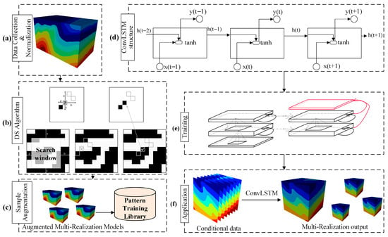
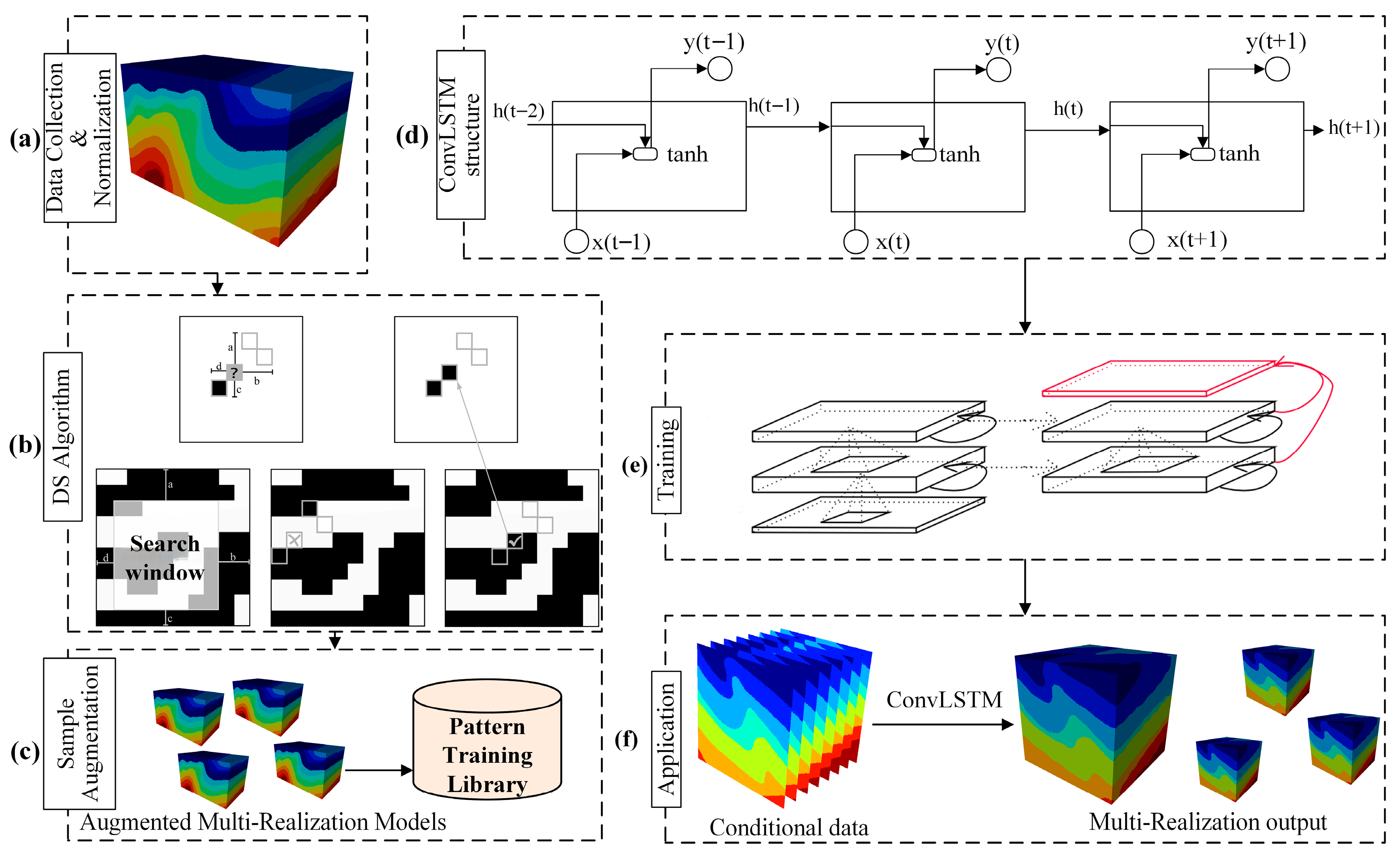
The proposed framework follows a unified and sequential workflow consisting of four main stages, data preparation, data preprocessing and representation, ConvLSTM model training, and 3D fold reconstruction and evaluation, as illustrated in Figure 1.

Figure 1. Workflow of the proposed method: (a) data preparation; (b) training data generation using the DS algorithm; (c) data serialization and representation; (d) ConvLSTM architecture; (e) model training; (f) 3D reconstruction and prediction.

Data Preparation. Heterogeneous geological data are collected and standardized to ensure consistency in spatial resolution, coordinate reference systems, and data quality. To construct a diverse and geologically realistic training dataset, the Direct Sampling (DS) algorithm is applied to generate multiple stochastic realizations from reference fold models. These realizations preserve the statistical and structural characteristics of the original data while introducing geometric variability. The resulting dataset covers a range of fold types and serves as the primary input for subsequent model training.

Data Preprocessing and Representation. All geological models are converted into a unified grid-based representation and stored in GSLIB format, which preserves spatial coordinates, grid resolution, and attribute values in a structured manner. This format facilitates data exchange and integration with geostatistical tools. For neural network processing, the 3D models are further serialized into sequences of 2D slices and organized into image-based formats, enabling efficient input into the ConvLSTM architecture while preserving spatial continuity.

ConvLSTM Model Training. The ConvLSTM network consists of an encoder, stacked ConvLSTM layers, and a decoder to capture both spatial and sequential dependencies in geological data. The model is trained using the generated datasets through iterative forward and backward propagation, with the mean squared error (MSE) serving as the loss function. An adaptive optimization algorithm is employed to update network parameters, while a validation subset and early-stopping strategy are used to monitor convergence and mitigate overfitting. The training process is conducted over a fixed number of epochs to ensure stable learning, and the optimized model parameters are retained for prediction.

3D Fold Reconstruction and Evaluation. After training, the ConvLSTM model takes sparse 2D geological profiles as input and predicts the corresponding 3D fold structures. The reconstructed models are quantitatively evaluated using multiple metrics, including structural similarity, spatial correlation, and modeling error (ε), to assess both geometric accuracy and geological plausibility.

2.2. Data Preparation

2.2.1. Training Datasets (Generated via DS Algorithm)

To construct a diverse and geologically realistic training dataset, the Direct Sampling (DS) algorithm [27] was employed as a data generation tool in the data preparation stage. The DS algorithm refers to a sampling-based approach that directly generates new realizations from existing geological data. Its core principle lies in simulating data events by directly sampling from the training image, rather than by constructing and storing a database of all possible data events. In the training image, MPS patterns with higher occurrence frequencies are more likely to be randomly accessed during the scanning process. Therefore, the probability of capturing a specific multi-point pattern directly from the training image is essentially consistent with that obtained by scanning the entire image and deriving it from the probability density function. Consequently, the DS algorithm enhances the quality and diversity of the training dataset, thereby improving the predictive capability and accuracy of the model.

For the DS algorithm, the most critical aspect is the quantification of pattern similarity. Pattern distance is introduced to measure the difference between two patterns. If patterns ${\mathrm{N}}_{\mathrm{u}}$ and ${\mathrm{N}}_{\mathrm{y}}$ are both composed of $\mathrm{n}$ nodes, the pattern distance is defined as

$$\mathrm{d}\left\{{\mathrm{N}}_{\mathrm{u}},{\mathrm{N}}_{\mathrm{y}}\right\}={\displaystyle \frac{1}{\mathrm{n}}}{\sum }_{\mathrm{i}=1}^{\mathrm{n}}{\mathrm{a}}_{\mathrm{i}}\in \left[0,1\right], \mathrm{while} {\mathrm{a}}_{\mathrm{i}}=\left\{\begin{array}{c}0, \mathrm{i}\mathrm{f} \mathrm{z}\left({\mathrm{u}}_{\mathrm{i}}\right)=\mathrm{z}\left({\mathrm{y}}_{\mathrm{i}}\right)\\ 1, \mathrm{i}\mathrm{f} \mathrm{z}\left({\mathrm{u}}_{\mathrm{i}}\right)\ne \mathrm{z}\left({\mathrm{y}}_{\mathrm{i}}\right)\end{array}.\right.$$

(1)

A perfectly matching pattern has a distance of 0, while a completely different pattern has a distance of 1. A distance threshold is used to determine whether a scanned pattern should be accepted as the simulation result, since some patterns cannot be matched exactly. The pattern-matching allows the DS algorithm to achieve high simulation efficiency while accurately reproducing geological patterns.

The DeeSse code is a parallel implementation based on the DS algorithm. It is controlled by three main parameters, t- distance threshold, n- number of neighboring nodes, and f- scan fraction [27] (https://github.com/randlab/geone (accessed on 5 October 2025)). The second parameter n defines the maximum number of nodes considered when comparing a pattern in the training images and in the simulation grid. The last parameter f allows to limit the simulation time while conserving realistic patterns reproduction. DeeSse excels at generating high-quality realizations but has limitations. It is highly sensitive to input data quality, with performance deteriorating in the presence of poor or sparse data. Additionally, DeeSse lacks flexibility, requiring significant parameter tuning for different geological contexts.

In this study, the DeeSse code was employed to expand the 3D fold dataset. Starting from an initial reference model (training image), multiple stochastic realizations were generated. Owing to the inherent randomness of MPS simulations, these realizations preserve similar geological characteristics while remaining non-identical, making them suitable as training samples for the ConvLSTM network [28,29].

Based on these generated realizations, a comprehensive training dataset was constructed using the DS algorithm to meet the requirements of ConvLSTM training. Specifically, expert-interpreted 3D fold models (64³ voxels) were used as training images, each representing a distinct fold category. These include horizontal upright, horizontal inclined, recumbent, plunging upright, plunging inclined, overturned, and vertical folds. Each model captures the corresponding morphological characteristics and spatial distribution patterns, as summarized in Table 1.

Table 1. Characteristic descriptions of different types of folds.

Fold Type	Characteristic Description
Horizontal upright fold	The axial plane is nearly vertical, and the hinge line is approximately horizontal.
Horizontal inclined fold	The axial plane is inclined, while the hinge line remains approximately horizontal.
Recumbent fold	Both the axial plane and hinge line are nearly horizontal.
Plunging upright fold	The axial plane is nearly vertical, and the hinge line plunges at an angle between 10° and 80°.
Plunging inclined fold	Both the axial plane and hinge line are inclined, but their dip directions and dip angles are not consistent.
Steep plunging fold	Both the axial-plane dip angle and hinge-line plunge angle range from 10° to 80°, and their dip directions are generally consistent.
Vertical fold	Both the axial plane and hinge line are nearly vertical.

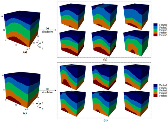
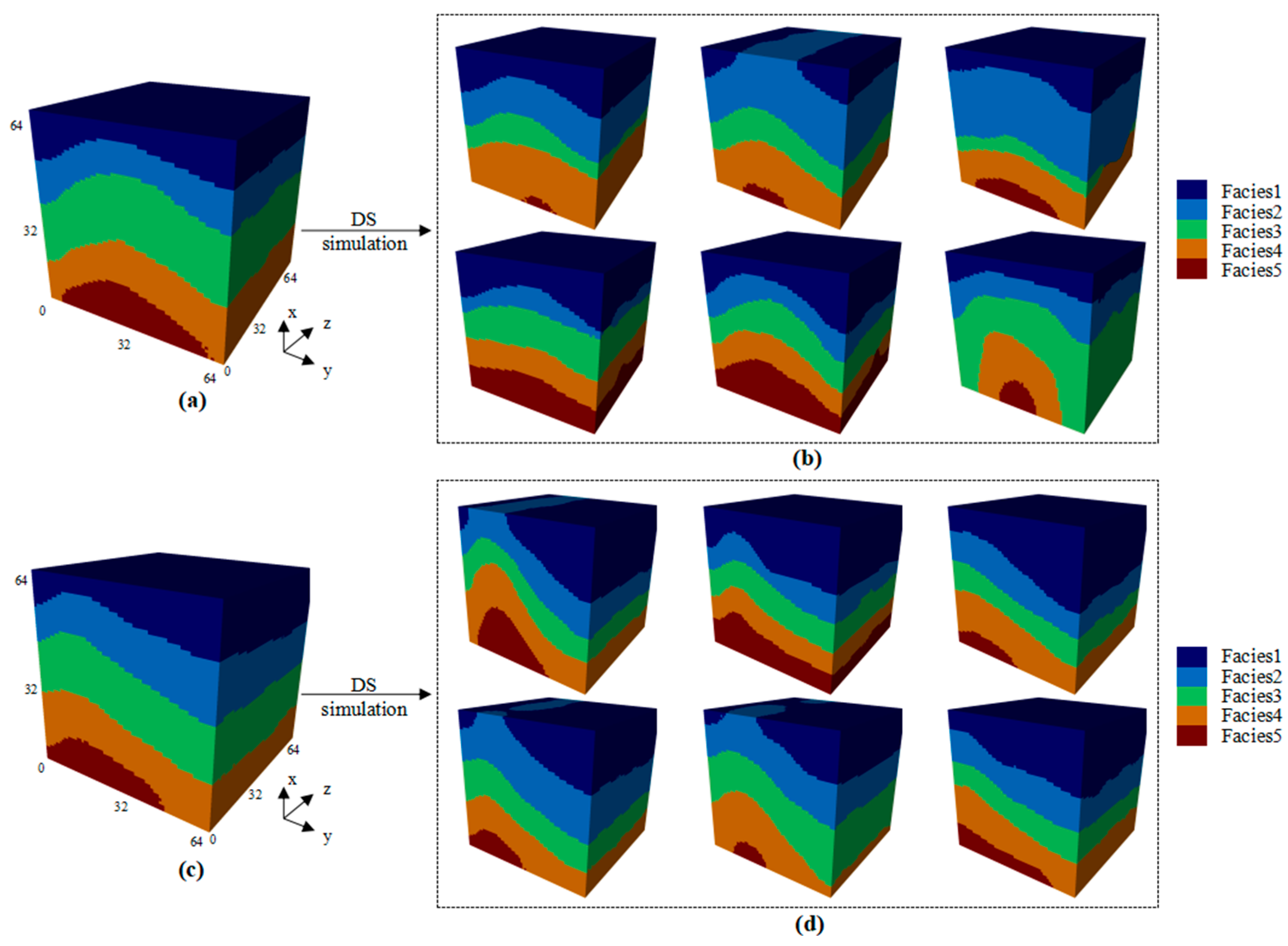
This section presents the experimental results using the horizontal upright fold and horizontal inclined fold as representative examples. As shown in Figure 2, Figure 2a depicts the expert-drawn horizontal upright fold model, which was used as the training image for simulation with the DS algorithm. Figure 2b visualizes six randomly selected 3D fold models generated from the simulation. Similarly, Figure 2c shows the expert-drawn horizontal inclined fold model, also used as a training image for DS-based simulation, and Figure 2d presents the corresponding simulated 3D fold models. The generated realizations preserve the statistical characteristics of the training images while exhibiting diverse morphologies. Furthermore, the study employed the DS algorithm to generate a total of 2000 simulated 3D fold model realizations, each with a resolution of 64³ voxels. The simulated dataset encompasses a variety of fold structures, covering different types and levels of geological complexity. It is designed to represent diverse geological scenarios, thereby providing high-quality foundational data for subsequent ConvLSTM model training.

Figure 2. Construction of 3D fold model training set. (a,c) are the different 3D training images provided by an expert; (b,d) are the constructed training set for ConvLSTM.

2.2.2. Validation Datasets

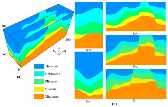
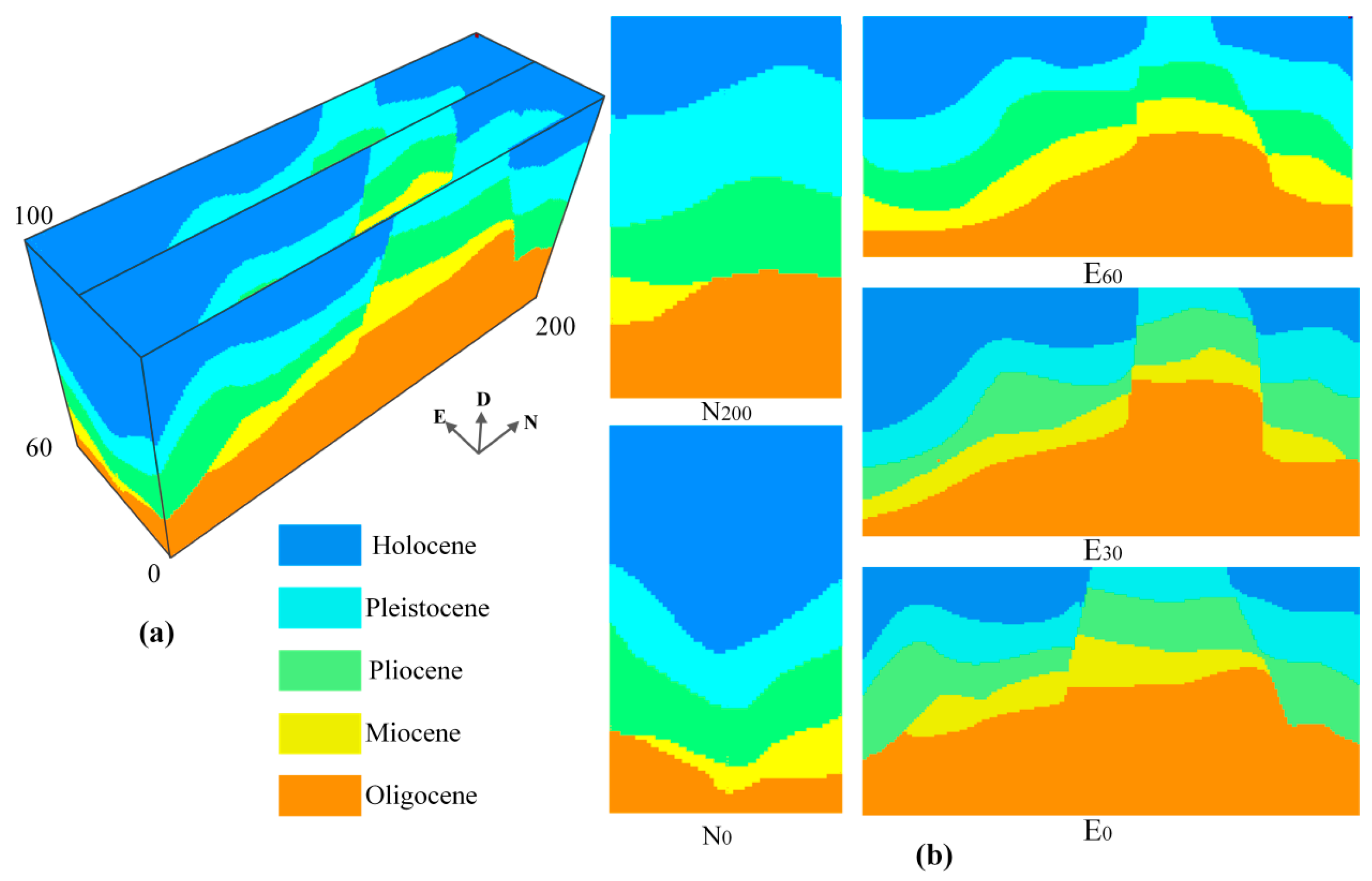
In this study, two types of datasets were used to validate the performance of the ConvLSTM model. The first dataset consists of three parallel profiles, supplemented by two orthogonal profiles, forming a sparse structural framework for 3D reconstruction. The delineated strata belonged to the Quaternary and Tertiary periods, ordered from top to bottom as the Holocene, Pleistocene, Pliocene, Miocene and Oligocene. As shown in Figure 3, wavy bedding was prevalent in the southern region, while two fault surfaces were located in the central region, forming an obvious fault drop. The central area showed relative uplift forming a horst. Towards the northern end of the two profiles, the Miocene stratum was lost, resulting in direct contact between the Oligocene and Pliocene strata. In the northern part of the central profile, the Miocene was pinched out. The Miocene stratum formed multiple pinch-outs in this area. In the experiment based on these three profiles, the 3D simulation grid was measured at 60 × 200 × 100 pixels.

Figure 3. Five known geological profiles with fold, faults and pinch-outs. (a) The 3D simulation grid and the color bar. (b) Fold morphology of five profiles and the corresponding number in the grid.

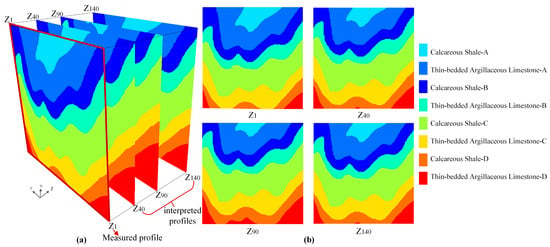
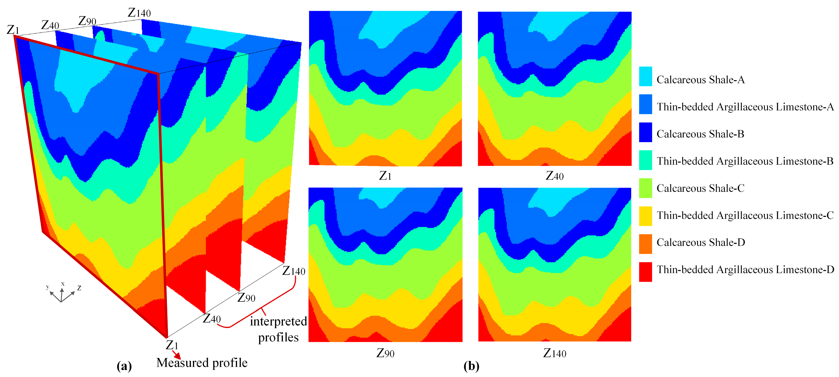
The second dataset came from the west bank of the Kali Gandaki River near Marpha Village, central Nepal (Coordinates: N 28°45′16.96″, E 83°40′42.77″). Field investigations focus on outcrops of the Silurian to Devonian Sombre Formation, which comprises calcareous shales that exhibit well-developed mesoscale F₂–F₃ fold interference patterns (Figure 4). These patterns provide critical evidence for a complex polyphase tectonic deformation history.

Figure 4. The measured profile Z1 and three interpreted profiles with the fold. (a) The 3D simulation grid. (b) Fold morphology of four profiles and the corresponding number in the grid.

The mesoscopic F₂ folds documented at Marpha are interpreted as parasitic structures associated with a crustal-scale, northeast-verging fold system. The dominant structure within this system is the spectacular, kilometer-scale Nilgiri anticline, which is prominently exposed on the western flank of the Nilgiri Mountains. This overturned antiform involves Ordovician limestones [27]. Macroscopic parasitic folds of the Nilgiri anticline include the Marpha anticline and the Jomsom syncline located farther north. Collectively, these structures constitute part of an extensive fold train that extends at least 50 km north of Kagbeni into the Upper Mustang region.

In the study area, we obtained a measured geological outcrop profile of Z1, as shown in Figure 4a, and selected a square area, which represents a 20 × 20 m² intense fold profile. At the positions corresponding to profiles Z40, Z90, and Z140, a total of 24 boreholes were drilled. These three profiles were constructed by integrating borehole lithological data with the stratigraphic patterns observed in profile Z1 and therefore represent interpreted profiles rather than direct observations. To validate the modeling performance of the aforementioned ConvLSTM, we constructed a three-dimensional fold model measuring 20 × 20 × 14 m³. These four parallel profiles, labeled Z1, Z40, Z90, and Z140 as shown in Figure 4, were employed in this case. Each profile has a resolution of 200 × 200 pixels.

2.2.3. Data Serialization

Assume that the original 3D geological data are represented as a tensor $\mathrm{V}\in {\mathrm{R}}^{\mathrm{H}\times \mathrm{W}\times \mathrm{D}}$, where $\mathrm{H}$, $\mathrm{W}$, $\mathrm{D}$ denote the height, width, and depth dimensions, respectively. To meet the input requirements of the ConvLSTM network (https://github.com/jhhuang96/ConvLSTM-PyTorch (accessed on 17 August 2025)), the tensor is evenly sliced along the depth axis D, generating a sequence of two-dimensional profiles $\left\{{\mathrm{x}}_1,{\mathrm{x}}_2,\cdots ,{\mathrm{x}}_{\mathrm{T}}\right\}$, where each ${\mathrm{x}}_{\mathrm{i}}\in {\mathrm{R}}^{\mathrm{H}\times \mathrm{W}}$ contains geological attribute information corresponding to a specific depth.

After normalization, the slice sequence is organized in spatiotemporal order into an input tensor $\mathrm{x}\in {\mathrm{R}}^{\mathrm{B}\times \mathrm{T}\times \mathrm{C}\times \mathrm{H}\times \mathrm{W}}$, where $\mathrm{B}$ denotes the batch size, $\mathrm{T}$ the number of time steps, and $\mathrm{C}$ the number of feature channels. This transformation converts the 3D spatial information into a temporally structured 2D sequence, thereby establishing the foundation for subsequent spatiotemporal modeling.

During model training, the complete 3D stratigraphic volume is used as both input and output to capture the implicit spatiotemporal dependencies between geological layers. During inference, only the surface slice ${\mathrm{x}}_1$ is required as input, and the model sequentially predicts the subsurface layers $\left\{{\mathrm{x}}_1^{\prime },{\mathrm{x}}_2^{\prime },\cdots ,{\mathrm{x}}_{\mathrm{T}}^{\prime }\right\}$, ultimately reconstructing the full 3D geological model ${\mathrm{V}}^{\mathrm{p}\mathrm{r}\mathrm{e}\mathrm{d}}\in {\mathrm{R}}^{\mathrm{H}\times \mathrm{W}\times \mathrm{D}}$. This approach enables a “2D observation to 3D inference” paradigm shift in geological modeling, substantially enhancing its applicability in data-limited subsurface scenarios.

2.3. Methodology

2.3.1. Convolutional LSTM Architecture

This study proposes a 3D geological fold modeling method based on a ConvLSTM network. The core idea is to conceptualize the spatial structure of a 3D geological body as a temporal evolutionary process, leveraging the powerful spatiotemporal sequence modeling capability of ConvLSTM to infer the complete 3D geological structure from limited two-dimensional geological slices. As illustrated in Figure 5, the proposed approach comprises four key stages: data preprocessing, feature encoding, sequence prediction, and 3D reconstruction. Together, these stages enable intelligent inference of complex geological structures from 2D observations to 3D representations.

Figure 5. The overall framework of the proposed ConvLSTM-based 3D fold modeling method.

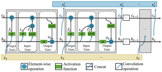
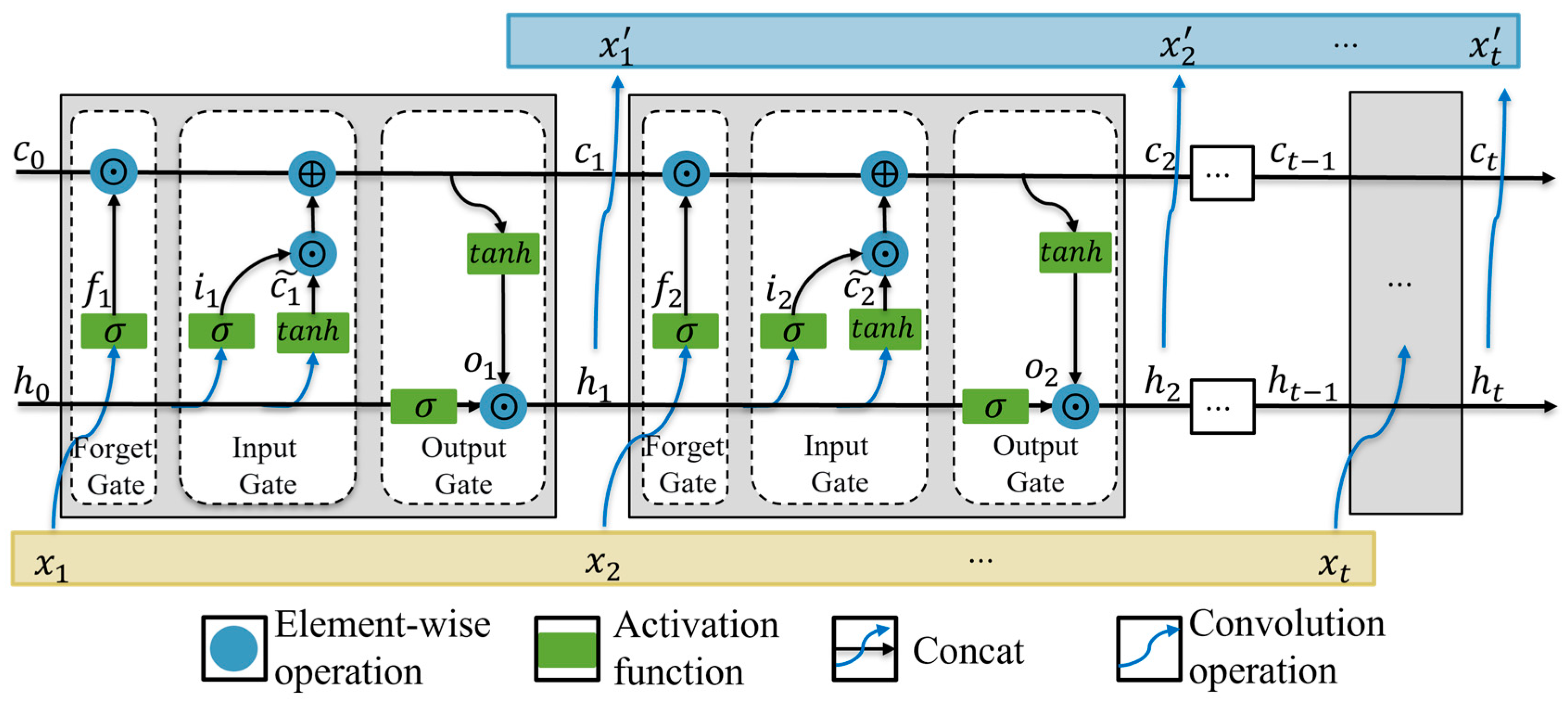
Traditional recurrent neural networks (RNNs) suffer from vanishing and exploding gradient problems when processing long sequences, which limits their applicability in geological time-series modeling [30,31]. The LSTM network addresses this challenge by introducing a sophisticated gating mechanism. The core innovation of the LSTM lies in its memory cell ${\mathrm{c}}_{\mathrm{t}}$, which acts as an accumulator of state information and manages information flow through three self-parameterized control gates.

Given an input sequence $\left\{{\mathrm{x}}_1,{\mathrm{x}}_2,\cdots ,{\mathrm{x}}_{\mathrm{T}}\right\}$, the computation process of the LSTM at time step $\mathrm{t}$ can be expressed as follows:

The forget gate determines how much of the previous state information should be retained:

$${\mathrm{f}}_{\mathrm{t}}=\mathsf{\sigma }\left({\mathrm{W}}_{\mathrm{f}}\cdot \left[{\mathrm{h}}_{\mathrm{t}-1},{\mathrm{x}}_{\mathrm{t}}\right]+{\mathrm{b}}_{\mathrm{f}}\right),$$

(2)

The input gate controls the inflow of new information:

$$\begin{array}{c}{\mathrm{i}}_{\mathrm{t}}=\mathsf{\sigma }\left({\mathrm{W}}_{\mathrm{i}}\cdot \left[{\mathrm{h}}_{\mathrm{t}-1},{\mathrm{x}}_{\mathrm{t}}\right]+{\mathrm{b}}_{\mathrm{i}}\right),\\ {\tilde{\mathrm{c}}}_{\mathrm{t}}=\tanh \left({\mathrm{W}}_{\mathrm{c}}\cdot \left[{\mathrm{h}}_{\mathrm{t}-1},{\mathrm{x}}_{\mathrm{t}}\right]+{\mathrm{b}}_{\mathrm{c}}\right).\end{array}$$

(3)

At each time step t, the LSTM cell receives a current input x_t: this is the element of the sequence at the current moment. For our geological modeling process, x_t represents the 2D geological slice at depth t, such as an image depicting stratigraphic sequences and thicknesses.

The memory cell is then updated as

$${\mathrm{c}}_{\mathrm{t}}={\mathrm{f}}_{\mathrm{t}}\odot {\mathrm{c}}_{\mathrm{t}-1}+{\mathrm{i}}_{\mathrm{t}}\odot {\tilde{\mathrm{c}}}_{\mathrm{t}}.$$

(4)

Finally, the output gate regulates the generation of the hidden state:

$$\begin{array}{c}{\mathrm{o}}_{\mathrm{t}}=\mathsf{\sigma }\left({\mathrm{W}}_{\mathrm{o}}\cdot \left[{\mathrm{h}}_{\mathrm{t}-1},{\mathrm{x}}_{\mathrm{t}}\right]+{\mathrm{b}}_{\mathrm{o}}\right),\\ {\mathrm{h}}_{\mathrm{t}}={\mathrm{o}}_{\mathrm{t}}\odot \tanh \left({\mathrm{c}}_{\mathrm{t}}\right).\end{array}$$

(5)

Here, $\mathsf{\sigma }$ denotes the sigmoid activation function, $\odot$ represents element-wise multiplication, and $\mathrm{W}$ and $\mathrm{b}$ are the weight matrices and bias terms, respectively. At each time step t, the LSTM cell outputs a current hidden state t, which synthesizes information from the current input x_t, the short-term memory h_t−1, and the long-term memory c_t−1 to extract the most relevant features for the current moment. For geological modeling, ht can be interpreted as the model’s “understanding” of the current depth slice x_t and its structural context. This hidden state t is then passed to the decoder to generate the predicted 2D geological slice.

Compared with conventional RNNs, the LSTM achieves precise control over the flow of information through its gating mechanism, effectively constraining gradient propagation within the memory cell and preserving long-term dependencies [31]. This significantly enhances its capability for modeling geological time-series data. However, the fully connected operations used in traditional LSTM architectures pose a limitation when processing spatial data: both the input-to-state and state-to-state transitions employ dense connections, which fail to capture local spatial correlations effectively, leading to redundant parameters and the loss of spatial structural information.

As a natural extension of the LSTM, the ConvLSTM network introduces convolutional operations into the recurrent structure. In ConvLSTM, all inputs, outputs, hidden states, and gating signals are represented as 3D tensors, with the last two dimensions corresponding to spatial coordinates (rows and columns). This design enables the future state of each grid cell to be determined jointly by the inputs and past states within its local spatial neighborhood, thereby making ConvLSTM particularly well suited for capturing the spatial continuity inherent in geological data.

The gating mechanisms in ConvLSTM are formulated using convolutional operations as follows:

$$\begin{array}{c}{\mathrm{f}}_{\mathrm{t}}=\mathsf{\sigma }\left({\mathrm{W}}_{\mathrm{f}}\ast {\mathrm{c}\mathrm{a}=\mathrm{t}(\mathrm{x}}_{\mathrm{t}},{\mathrm{h}}_{\mathrm{t}-1})+{\mathrm{b}}_{\mathrm{f}}\right),\\ {\mathrm{i}}_{\mathrm{t}}=\mathsf{\sigma }\left({\mathrm{W}}_{\mathrm{i}}\ast {\mathrm{c}\mathrm{a}\mathrm{t}(\mathrm{x}}_{\mathrm{t}},{\mathrm{h}}_{\mathrm{t}-1})+{\mathrm{b}}_{\mathrm{i}}\right),\\ \begin{array}{c}\widetilde{{\mathrm{c}}_{\mathrm{t}}}=\mathrm{t}\mathrm{a}\mathrm{n}\mathrm{h}\left({\mathrm{W}}_{\mathrm{c}}\ast {\mathrm{c}\mathrm{a}\mathrm{t}(\mathrm{x}}_{\mathrm{t}},{\mathrm{h}}_{\mathrm{t}-1})+{\mathrm{b}}_{\mathrm{c}}\right),\\ \begin{array}{c}{\mathrm{o}}_{\mathrm{t}}=\mathsf{\sigma }\left({\mathrm{W}}_{\mathrm{o}}\ast {\mathrm{c}\mathrm{a}\mathrm{t}(\mathrm{x}}_{\mathrm{t}},{\mathrm{h}}_{\mathrm{t}-1})+{\mathrm{b}}_{\mathrm{o}}\right),\\ {\mathrm{c}}_{\mathrm{t}}={\mathrm{f}}_{\mathrm{t}}\odot {\mathrm{c}}_{\mathrm{t}-1}+{\mathrm{i}}_{\mathrm{t}}\odot \widetilde{{\mathrm{c}}_{\mathrm{t}}},\\ {\mathrm{h}}_{\mathrm{t}}={\mathrm{o}}_{\mathrm{t}}\odot \tanh \left({\mathrm{c}}_{\mathrm{t}}\right).\end{array}\end{array}\end{array}$$

(6)

where $\ast$ denotes the convolution operation, $\odot$ represents the Hadamard (element-wise) product, $\mathsf{\sigma }$ is the sigmoid activation function, and $\mathrm{c}\mathrm{a}\mathrm{t}$ indicates channel-wise concatenation.

Compared with the fully connected LSTM, the ConvLSTM treats the input ${\mathrm{x}}_{\mathrm{t}}$, hidden state ${\mathrm{h}}_{\mathrm{t}}$, and memory cell ${\mathrm{c}}_{\mathrm{t}}$ as 3D tensors of size ($\mathrm{B}\times \mathrm{H}\times \mathrm{W}\times \mathrm{C}$), thereby preserving spatial neighborhood information through convolutional computations. The initial hidden state ${\mathrm{h}}_0$ and memory cell ${\mathrm{c}}_0$ are initialized with Gaussian random noise and are optimized automatically during training via backpropagation.

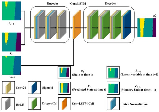
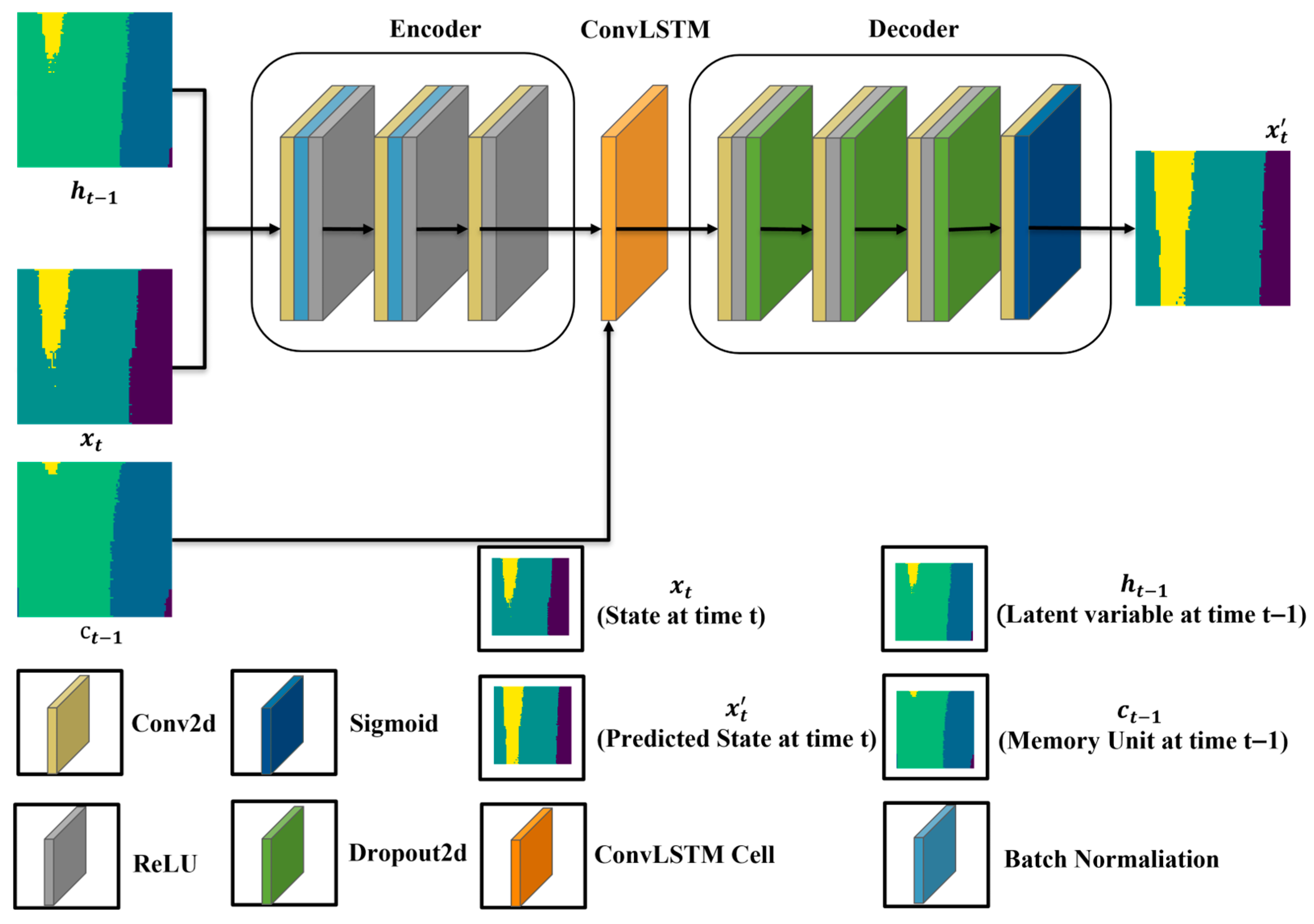
In this study, an encoder–decoder architecture is employed to perform sequence-to-sequence prediction from two-dimensional slices to subsequent slices. The framework consists of three main components: an encoder module, a ConvLSTM module, and a decoder module. The encoder is designed to extract joint spatiotemporal features from both the input slice sequence and the latent variable sequence. The ConvLSTM module further integrates these extracted spatiotemporal feature maps with the memory states to capture dynamic dependencies over depth. Finally, the decoder module maps the predicted feature representations back to the corresponding output slice sequence. The detailed network structure is illustrated in Figure 6, which shows the data flow from input slices through feature extraction, spatiotemporal modeling, and final slice prediction.

Figure 6. Encoder–decoder architecture used in the proposed ConvLSTM-based geological modeling framework.

Given an initial slice sequence $\left\{{\mathrm{x}}_1,{\mathrm{x}}_2,\cdots ,{\mathrm{x}}_{\mathrm{T}}\right\}$, an initial latent variable ${\mathrm{h}}_0$, and an initial memory cell ${\mathrm{c}}_0$, the encoder, ConvLSTM, and decoder modules are denoted as mappings ${\mathrm{f}}_{\mathrm{e}},{\mathrm{f}}_{\mathrm{L}}$ and ${\mathrm{f}}_{\mathrm{d}}$, respectively. The sequential update process can thus be formulated as

$${\mathrm{h}}_{\mathrm{i}},{\mathrm{c}}_{\mathrm{i}}={\mathrm{f}}_{\mathrm{L}}\left({\mathrm{f}}_{\mathrm{e}}\left({\mathrm{x}}_{\mathrm{i}},{\mathrm{h}}_{\mathrm{i}-1}\right),{\mathrm{c}}_{\mathrm{i}-1}\right),\mathrm{i}=1,2,\cdots ,\mathrm{T}.$$

(7)

Subsequently, the predicted input sequence is obtained as

$${\mathrm{x}}_{\mathrm{i}}^{\prime }={\mathrm{f}}_{\mathrm{d}}\left({\mathrm{h}}_{\mathrm{i}}\right),\mathrm{i}=1,2,\cdots ,\mathrm{T}.$$

(8)

Finally, the decoder outputs the predicted slice ${\mathrm{x}}_{\mathrm{i}}^{\prime }\in {\mathrm{R}}^{\mathrm{H}\times \mathrm{W}}$, where the output values are constrained within the range [0, 1] through a sigmoid activation function.

2.3.2. Network Training and 3D Reconstruction

To achieve high-precision 3D stratigraphic prediction, this study designs a multi-objective loss function that jointly optimizes structural consistency and categorical accuracy. The overall loss function is defined as

$${\mathcal{L}}_{\mathrm{t}\mathrm{o}\mathrm{t}\mathrm{a}\mathrm{l}}={\mathsf{\lambda }}_1{\mathcal{L}}_{\mathrm{r}\mathrm{e}\mathrm{c}}+{\mathsf{\lambda }}_2{\mathcal{L}}_{\mathrm{s}\mathrm{s}\mathrm{i}\mathrm{m}}.$$

(9)

where ${\mathcal{L}}_{\mathrm{r}\mathrm{e}\mathrm{c}}={∥{\mathrm{x}}_{\mathrm{t}}^{\prime }-{\mathrm{x}}_{\mathrm{t}}∥}^2$ represents the pixel-wise reconstruction loss and ${\mathcal{L}}_{\mathrm{s}\mathrm{s}\mathrm{i}\mathrm{m}}$ quantifies the structural similarity between the predicted and true slices, thereby enhancing the discrete stratigraphic classification accuracy. The coefficients ${\mathsf{\lambda }}_1,{\mathsf{\lambda }}_2$ are weighting parameters balancing the two objectives. The Adam optimizer is employed to accelerate convergence, with a dynamically adjusted learning rate to prevent gradient oscillation.

After model training, the surface slice ${\mathrm{x}}_1$ is used as the initial state, and the ConvLSTM recursively generates subsurface prediction slices in a stepwise manner. The final 3D geological model is obtained by sequentially stacking the predicted slices:

$${\mathrm{V}}^{\mathrm{p}\mathrm{r}\mathrm{e}\mathrm{d}}\left(\mathrm{x},\mathrm{y},\mathrm{z}\right)=\mathrm{Stack}\left({\mathrm{x}}_{\mathrm{i}}^{\prime }\right),\mathrm{i}=1,2,\cdots ,\mathrm{T}.$$

(10)

Post-processing is performed using trilinear interpolation and morphological filtering to smooth stratigraphic interfaces and remove isolated noise artifacts. This method enables automatic generation of 3D stratigraphic models that conform to geological structural patterns, relying solely on two-dimensional surface information. It thus establishes a new paradigm for geological modeling based on deep spatiotemporal learning.

2.4. Experimental Setup

The proposed ConvLSTM-based 3D fold modeling framework was implemented using PyTorch 1.12 and Python 3.9. Network parameters were optimized with the Adam optimizer. All experiments were conducted on a workstation equipped with an Intel Comet Lake 3.3 GHz CPU, 24 GB RAM, and an NVIDIA GeForce RTX 3090 GPU. Detailed network architecture parameters are provided in Table 2, Table 3 and Table 4. The hyperparameters ${\lambda }_1,{\lambda }_2$ in the loss function (${\lambda }_1$ = 0.4 for reconstruction loss, ${\lambda }_2$ = 0.6 for structural similarity loss) were determined empirically through preliminary experiments. We tested several ratio combinations (e.g., 0.2/0.8, 0.5/0.5, 0.6/0.4) on a validation set and found that 0.4/0.6 achieved the best balance between pixel-wise accuracy and structural continuity. A higher weight on structural similarity (${\lambda }_2$) was intentionally chosen because preserving geological layer continuity and fold geometry is more critical in our application than exact pixel-level matching.

Table 2. Network Configuration of the Encoder.

Type	Kernel Size/Padding	Input Feature Dimension	Output Feature Dimension	BN	Activation Function
Conv2d	3 $\times$ 3/1	1	32	$\surd$	ReLU
Conv2d	3 $\times$ 3/1	32	32	$\surd$	ReLU
Conv2d	3 $\times$ 3/1	32	16	$\times$	ReLU

Table 3. ConvLSTM Network Configuration.

Type	Kernel Size/Padding	Input Feature Dimension	Output Feature Dimension	BN	Activation Function
Conv2d	3 $\times$ 3/1	32	64	$\surd$	ReLU
Conv2d	3 $\times$ 3/1	64	64	$\times$	ReLU

Table 4. Network Configuration for the Decoder.

Type	Kernel Size/Padding	Input Feature Dimension	Output Feature Dimension	Dropout	Activation Function
Conv2d	3 $\times$ 3/1	16	32	$\surd$	ReLU
Conv2d	3 $\times$ 3/1	32	64	$\surd$	ReLU
Conv2d	3 $\times$ 3/1	64	32	$\surd$	ReLU
Conv2d	3 $\times$ 3/1	32	1	$\times$	Sigmoid

The learning rate of 1 × 10⁻⁴ was selected based on common practice for Adam optimizer in image-based deep learning tasks, and we confirmed its stability through initial training runs where loss decreased smoothly without oscillation. The 50-epoch training duration was determined by monitoring validation loss—beyond 50 epochs, we observed no significant improvement, and slight overfitting began to occur.

All code compilation, geostatistical modeling, experimental analysis, and visualization were performed using PyCharm 2025.3.3 (JetBrains s.r.o., Prague, Czech Republic), SGeMS 2.5 (Stanford University, Stanford, CA, USA), and ParaView 6.0.0 (Kitware, Inc., Clarksville, MD, USA).

2.5. Evaluation Metrics

For the 3D model constructed in this study, we used property proportion distribution, slice visualization, analysis of variation and connectivity, structural similarity measurement, and information entropy to evaluate the model’s accuracy and uncertainty. The relevant methods are described below.

Connectivity of a geological model refers to the physical linkage between different units or components and is quantified using a connectivity function. The connectivity function evaluates the probability that two points separated by a specific distance belong to the same connected region within the model. The variogram, on the other hand, characterizes the spatial variability of a regionalized variable, such as a geological property, reflecting how the degree of spatial variation changes with distance. It provides a quantitative measure of the spatial heterogeneity of regionalized variables. The variogram is calculated using the following formula:

$$\mathsf{\gamma }\left(\mathrm{r}\right)={\displaystyle \frac{1}{2\mathrm{N}\left(\mathrm{r}\right)}}{\sum }_{\mathrm{i}=1}^{\mathrm{N}\left(\mathrm{r}\right)}{\left(\mathrm{Z}({\mathrm{p}}_{\mathrm{i}}+\mathrm{r})-\mathrm{Z}({\mathrm{p}}_{\mathrm{i}})\right)}^2$$

(11)

Here, $\mathrm{N}(\mathrm{r})$ denotes the number of point pairs separated by a distance r; ${\mathrm{p}}_{\mathrm{i}}$ represents the coordinates of the i-th pixel; ${\mathrm{p}}_{\mathrm{i}}$ is the attribute value at that point; and $\mathrm{Z}({\mathrm{p}}_{\mathrm{i}}+\mathrm{r})$ is the attribute value at a point located a distance r away from pi. By varying the distance r, a series of variogram values can be computed. Plotting these values with r on the horizontal axis and $\mathsf{\gamma }(\mathrm{r})$ on the vertical axis yields the variogram curve.

Structural similarity (SSIM) is employed to evaluate the structural consistency between the training images and their neighboring reconstructed profiles and to identify regions with higher structural uncertainty.

Information entropy is used to quantitatively evaluate the residual uncertainty of the reconstructed geological structures relative to known geological information. This analysis measures the entropy difference between the actual and simulated profiles in terms of lithological distribution, as well as the conditional entropy of the simulated profile given the reference profile and the mutual information between the two. A smaller entropy difference and lower conditional entropy indicate a higher level of structural consistency between the simulated and reference profiles, whereas larger mutual information reflects a stronger correspondence between the reconstructed structures and the known geological patterns [22].

3. Results and Analysis

Based on the above-mentioned datasets, a set of experimental results and a case study are presented in this section.

3.1. Experimental Results

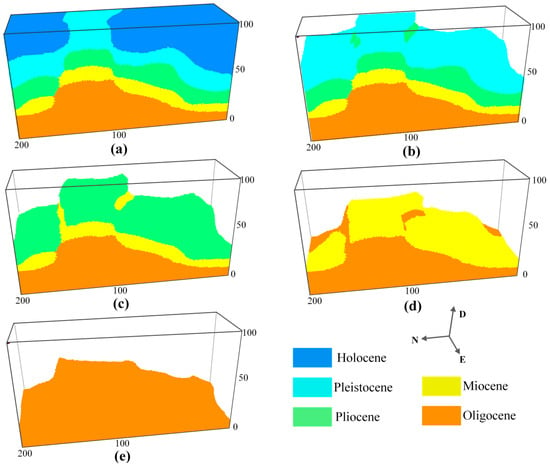
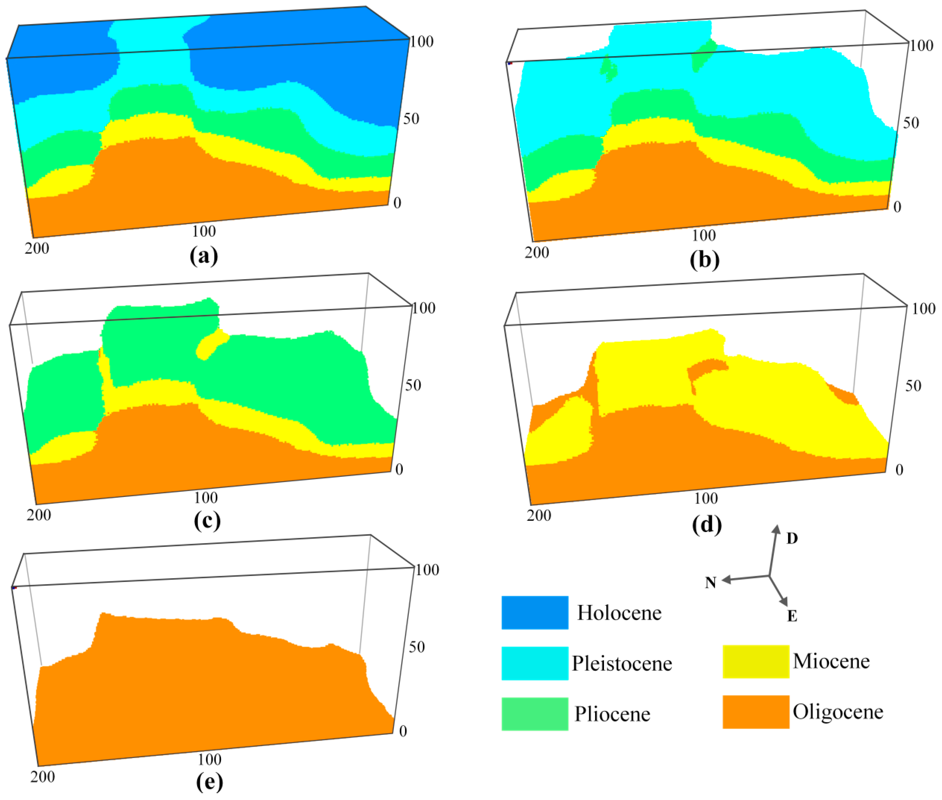
Figure 7 delineates the precise morphology of each stratum in the 3D reconstructed model. In the reconstructed model, the Oligocene and the Pliocene strata directly contact each other in the northwest due to the loss of the Miocene stratum, while the five strata in the northeast remained intact. A horst was evident in the middle, with distinct fault surfaces flanking its sides. On the north side of the horst, the Miocene and the Pliocene strata were completely separated, while the Pleistocene stratum remained partially connected. The fault on the south side of the horst exhibited a relatively gentle inclination, and to the east of the fault, the Miocene stratum was in direct contact with the Pliocene stratum. However, this connection gradually diminished as the fault extended westwards.

Figure 7. The spatial morphology of each stratum in the reconstructed 3D stratigraphic model. (a–e) Different morphologies of five strata in the 3D stratigraphic model.

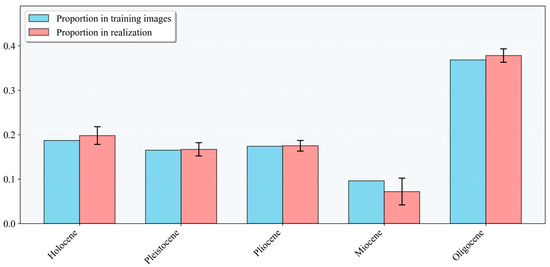
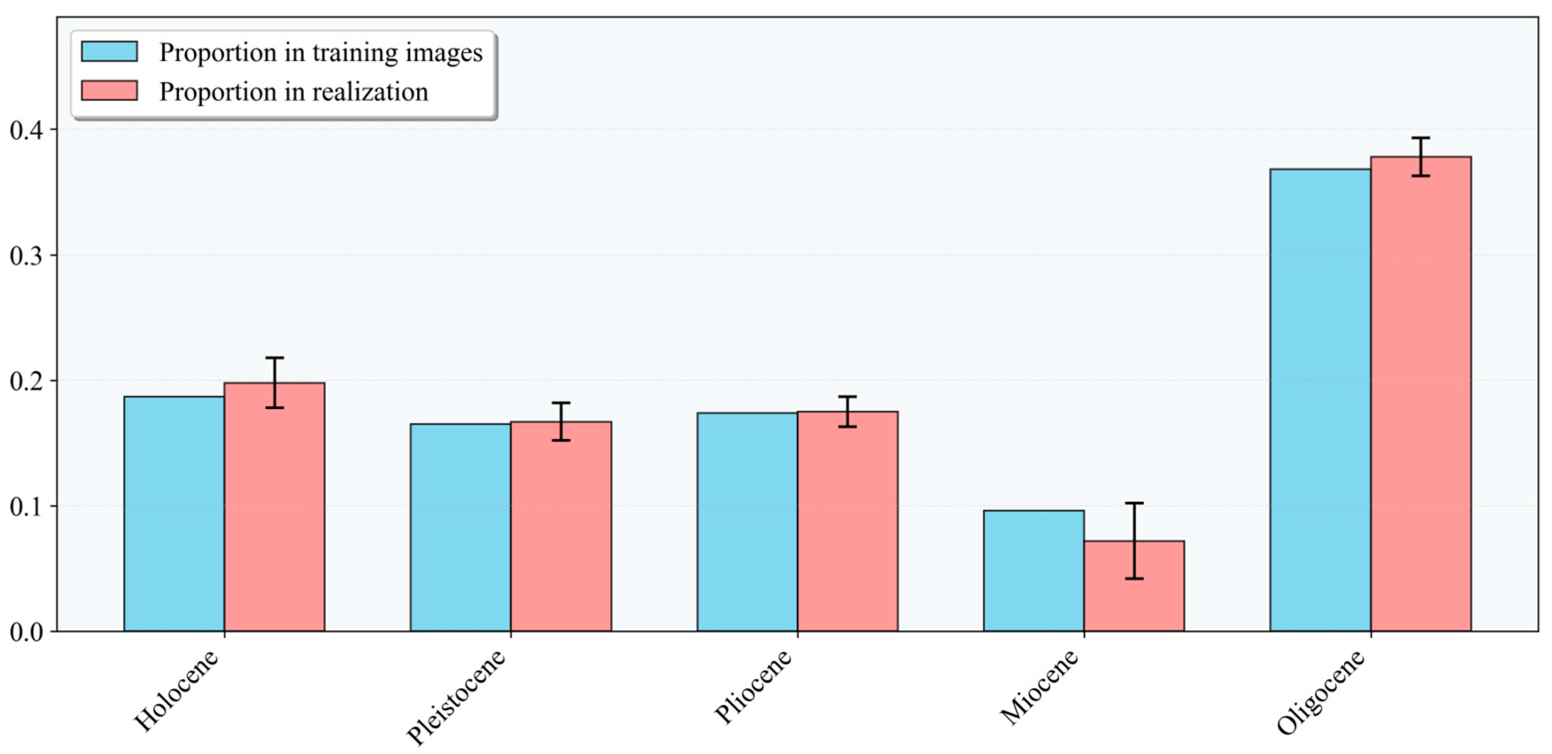
As depicted in Figure 8, we calculated the proportion of each stratum within both the training images and the 3D realization and then normalized the values. The proportions of Holocene, Pleistocene, Pliocene, and Oligocene strata exhibited variations of less than 2%, whereas the proportion of the Miocene stratum showed a change of 2.4%.

Figure 8. Proportion comparison of training images and the corresponding reconstructed models.

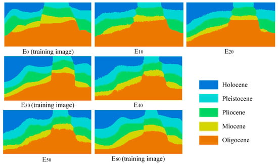
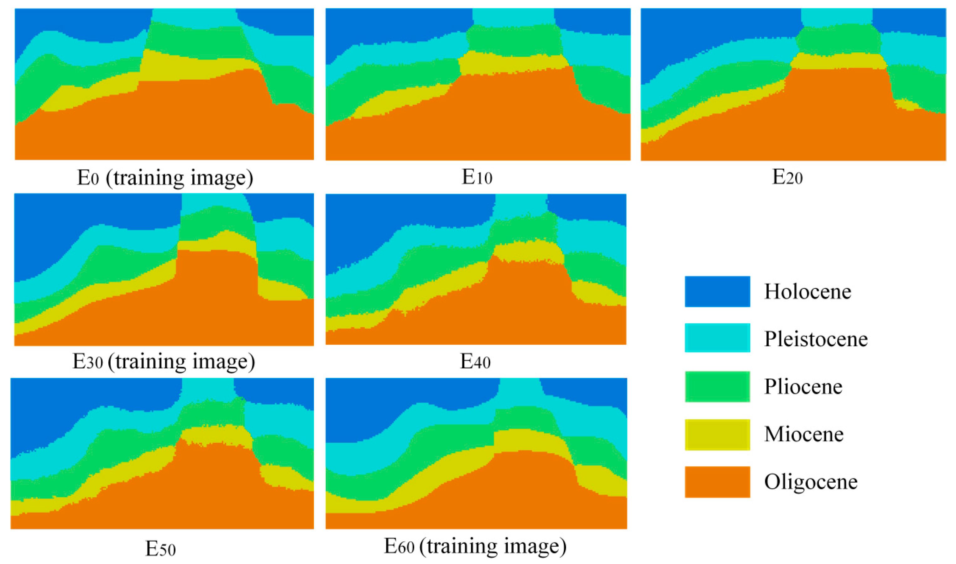
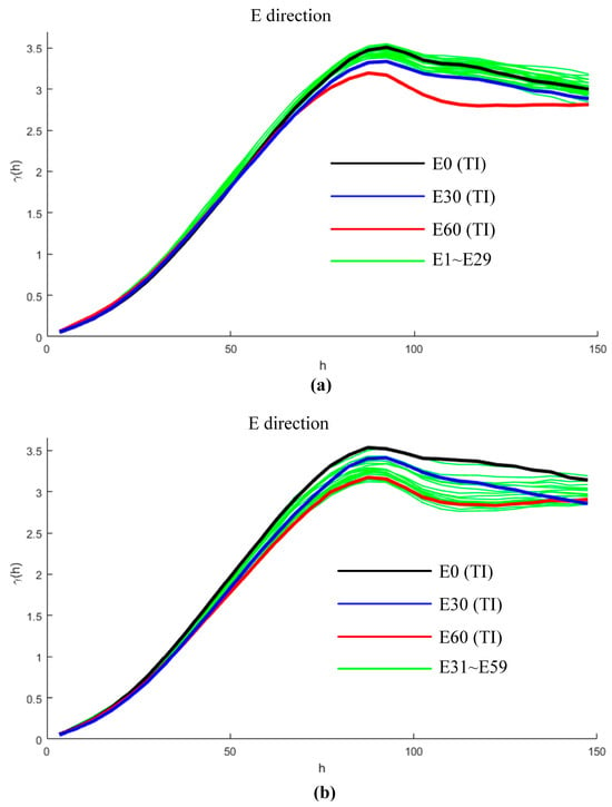
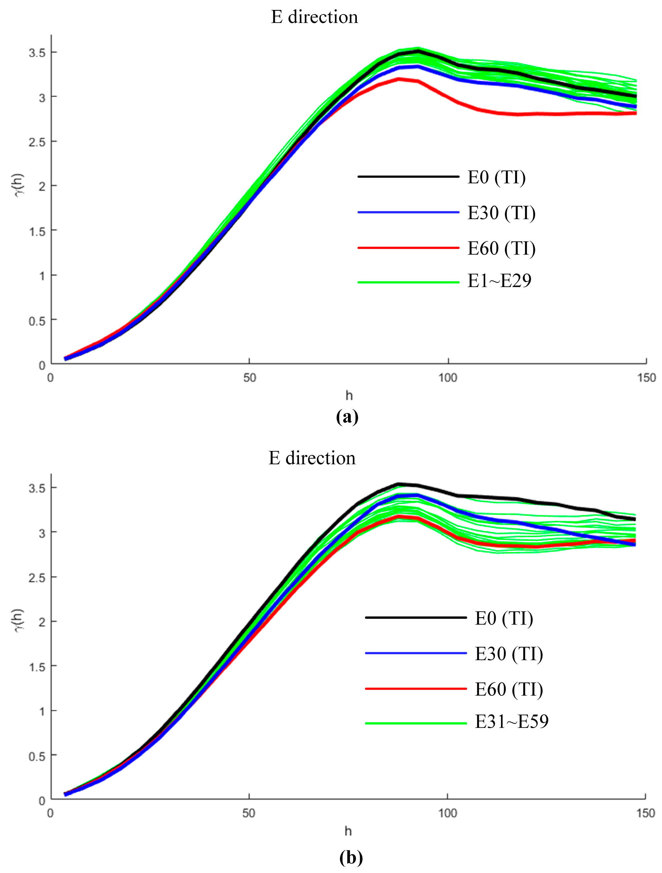
To further analyze the continuous changes in strata in different profiles, we selected 10 vertical profiles in the 3D model from east to west. Figure 9 illustrates that the morphology of each stratum was well reproduced by comparing the new profiles with the conditioning profiles. In Figure 10, the variograms of the three training images E0, E30 and E60 are described by black, blue and red curves, respectively. The green curves in Figure 10a,b represent the variograms of generated profiles from E1 to E29 and from E31 to E59, respectively. The curves from E1 to E29 lie between the curves E0 and E30, while the curves from E31 to E59 lie between the curves E30 and E60. This observation suggests that AS3DR is capable of capturing statistical characteristics across multiple training images smoothly.

Figure 9. Seven vertical slices of the reconstructed 3D model from east to west.

Figure 10. Variograms of the training images and the vertical reconstructed profiles. (a) Curves of the training images and reconstructed profiles from E1 to E29; (b) curves of the training images and the reconstructed profiles from E31 to E59.

As we can see from Figure 10, the statistical characteristics of the generated intermediate profiles are between those of their adjacent known profiles. This indicates that the generated profiles have stable variation characteristics, with a natural transition of geological attributes, and that these profiles do not overfit the known profiles.

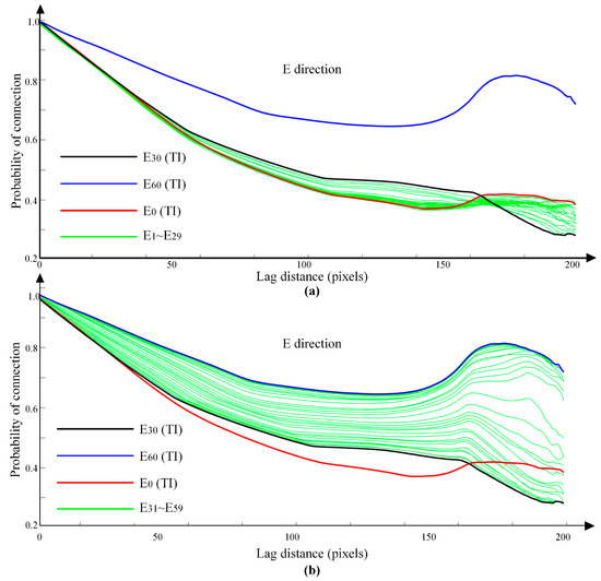
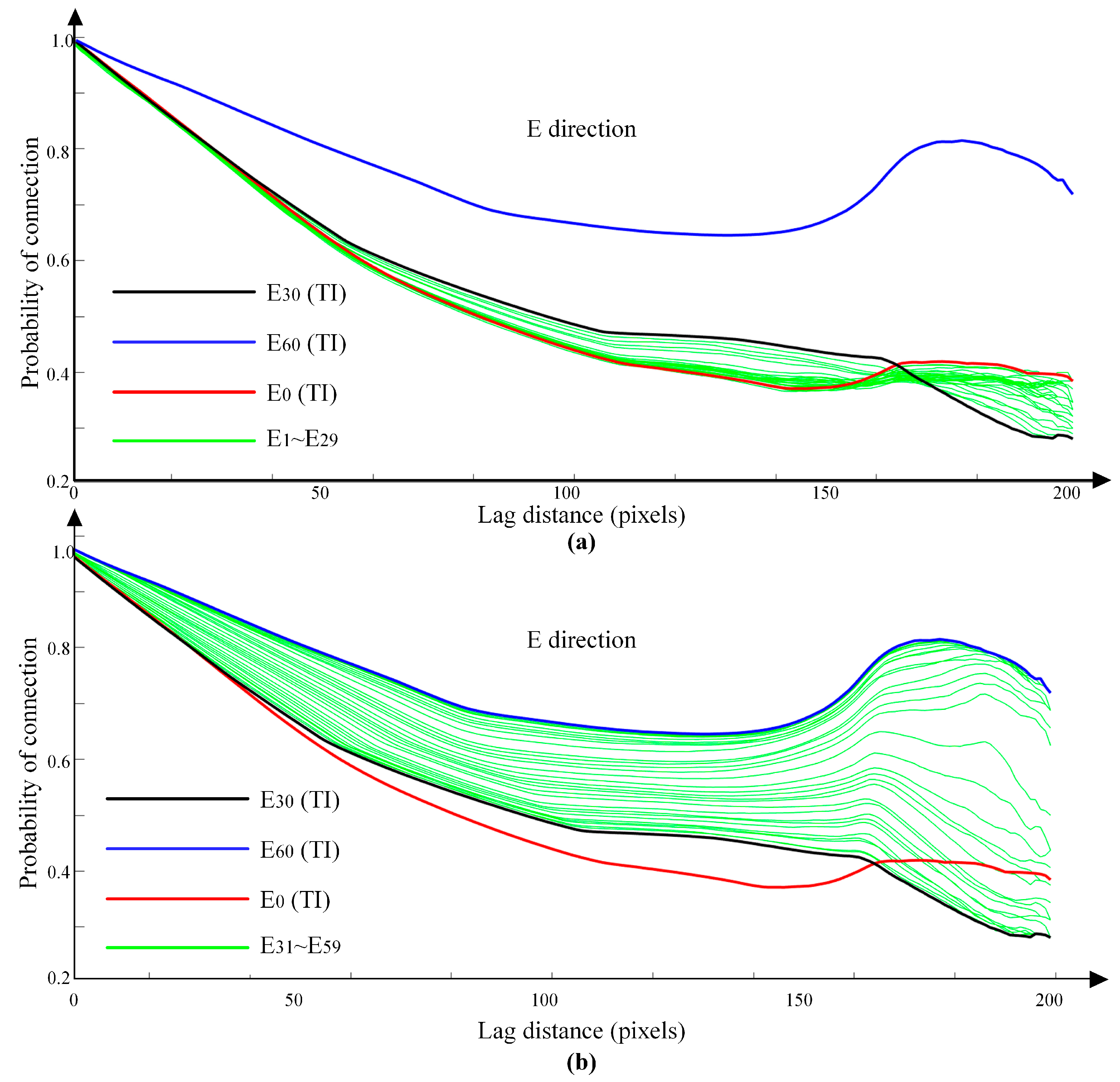
We focused our analysis on the Pliocene stratum to evaluate the connectivity between the training images and the corresponding realizations. The connectivity curves of the Pliocene stratum in the three training images E0, E30, and E60 are illustrated with red, black, and blue curves, respectively, in Figure 11. In addition, the green curves in Figure 11a depict the connectivity of the Pliocene stratum across profiles from E1 to E29. Similarly, the green curves in Figure 11b represent the profiles E31 to E59. Figure 10 reveals that the connectivity curves of the training images exhibited distinct characteristics, which indicated substantial morphological variation within the single stratum. The connectivity curves of the reconstructed profiles positioned themselves between the curves of the adjacent two training images, signifying a gradual and seamless transition. This proves that the specific stratum in the reconstructed model showed a high degree of consistency with the connectivity features of the original training images.

Figure 11. Analysis of connectivity of the Pliocene stratum. (a) Comparisons of the curves of the profiles from E1 to E29 and the three training images. (b) Comparisons of the curves of the profiles from E31 to E59 and three training images.

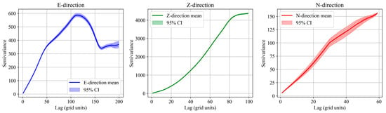
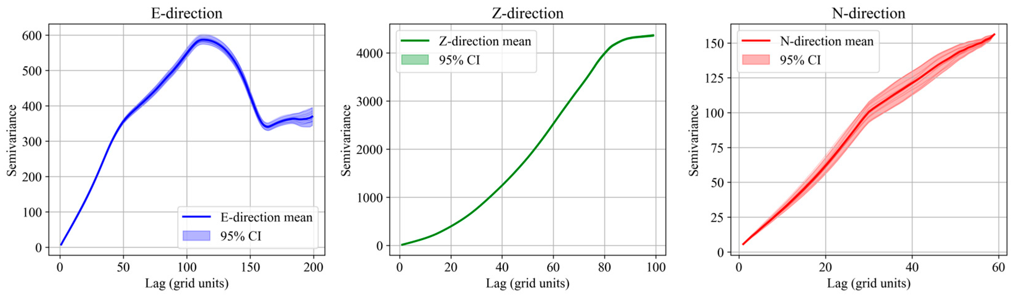
To evaluate the statistical variability among different stochastic realizations, we generated ten 3D models and computed their experimental variograms in the three principal directions. As shown in Figure 12, the variogram curves from all ten models are nearly superimposed, and the 95% confidence intervals (shaded areas) are extremely narrow, indicating that the models exhibit highly consistent spatial statistical characteristics. Combined with the previous analysis of feature differences among different slices within the same model, these results demonstrate that our method can accurately reproduce complex stratigraphic structures and possesses excellent stability.

Figure 12. Variogram analysis of 10 3D models with 95% confidence intervals (CI).

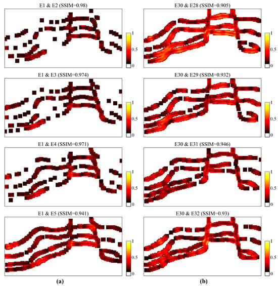
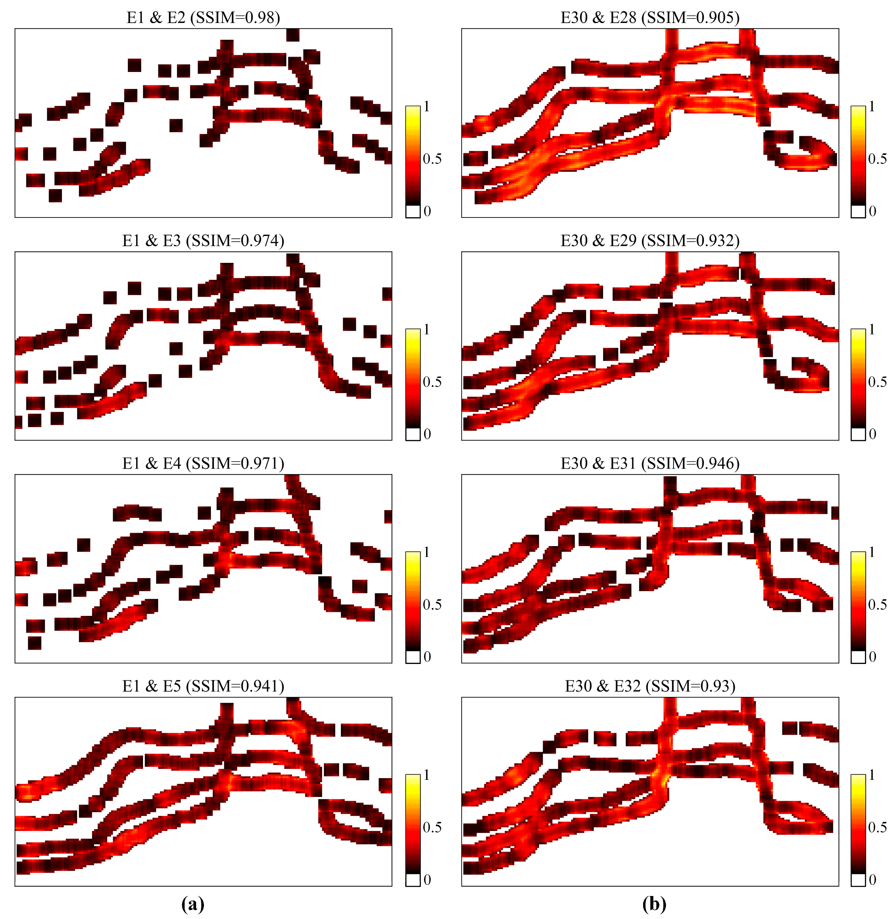
Figure 13 presents the SSIM maps comparing the training images (E1 and E30) with several adjacent reconstructed profiles extracted from the two sets of 3D realizations. In the SSIM index maps, white represents complete agreement between the profiles, whereas brighter regions indicate larger structural discrepancies. As shown in Figure 13, the structural similarity between the training images and the reconstructed profiles generally exceeds 90%, indicating that the reconstructed profiles preserve the main stratigraphic structures of the training images. The regions with relatively lower similarity mainly appear along stratigraphic boundaries, where slight positional variations in lithological interfaces occur during the reconstruction process. These localized variations reflect the inherent uncertainty of geological structure reconstruction rather than systematic modeling errors, and their orderly distribution suggests that the proposed method maintains stable stratigraphic continuity during the generation of intermediate profiles.

Figure 13. SSIM-based structural similarity analysis between training images and nearby reconstructed profiles in the 3D realizations. (a) SSIM comparison between training image E1 and adjacent reconstructed profiles E2–E5. (b) SSIM comparison between training image E30 and adjacent reconstructed profiles E28–E32.

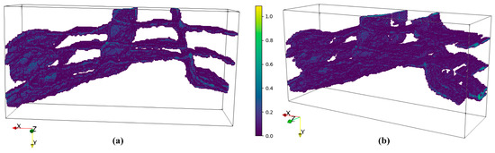
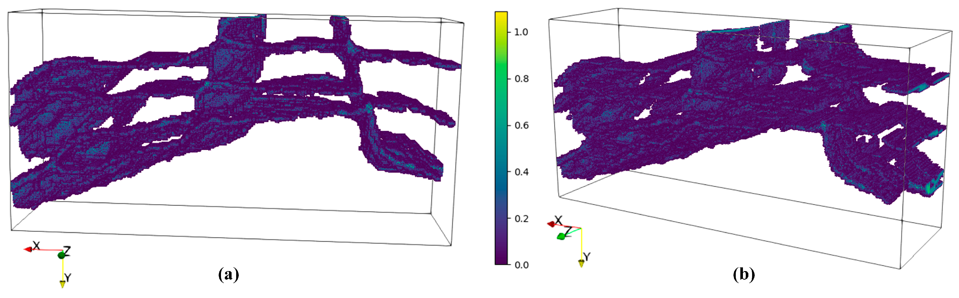
To better analyze the stability of our proposed method and the uncertainty of the generated 3D models, we plotted information entropy diagrams based on 10 3D models. As shown in Figure 14, the model uncertainty mainly originates from stratigraphic boundaries, and the entropy values are generally low. In previous model slices, we have already verified the correctness of the sequence reconstruction; overall, the model uncertainty is under control.

Figure 14. Uncertainty Analysis of 3D Models Based on Information Entropy. (a,b) show different perspectives.

The above analyses indicate that ConvLSTM performs well in fold modeling even when complex structural features, such as faults, are present, demonstrating the effectiveness and robustness of the proposed approach. Therefore, the ConvLSTM-based 3D fold-modeling method holds broad application potential in geological exploration, hazard prediction, and resource management and can effectively support practical geological modeling tasks.

3.2. Case Study

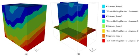
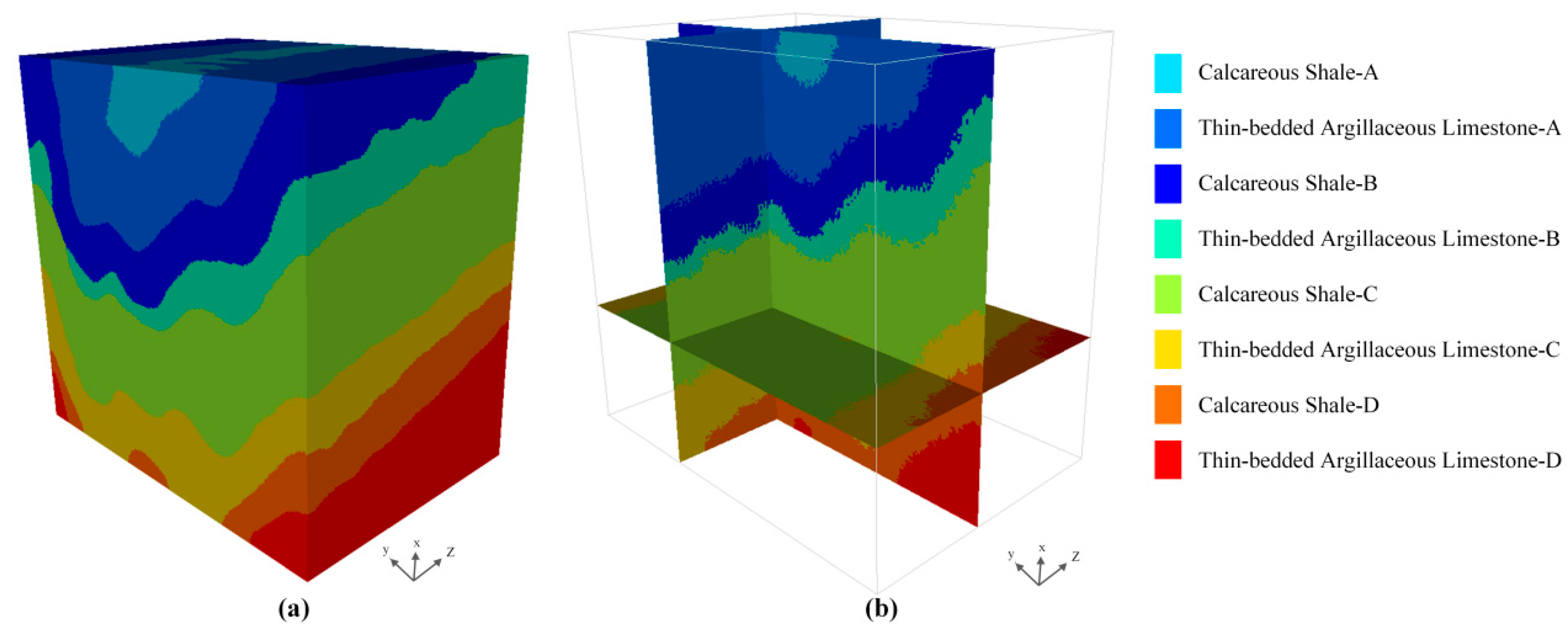
Based on the above-mentioned datasets, ten 3D fold models were generated using the trained LSTM model. One model was randomly selected for demonstration in this section, as shown in Figure 15. The model exhibits good stratigraphic continuity, well-defined interlayer contacts, and naturally varying layer geometries. The fold’s axial surfaces and stratigraphic relationships correspond closely with the two-dimensional profiles presented in Figure 4, effectively capturing the characteristics of the corresponding folds. On the basis of fidelity to the measured profile (Z1) and three interpreted profiles (Z40, Z90, Z140), the model provides an accurate reconstruction of the regional stratigraphy.

Figure 15. 3D fold model constructed by ConvLSTM. (a) 3D reconstructed model; (b) slice of the 3D model from three directions.

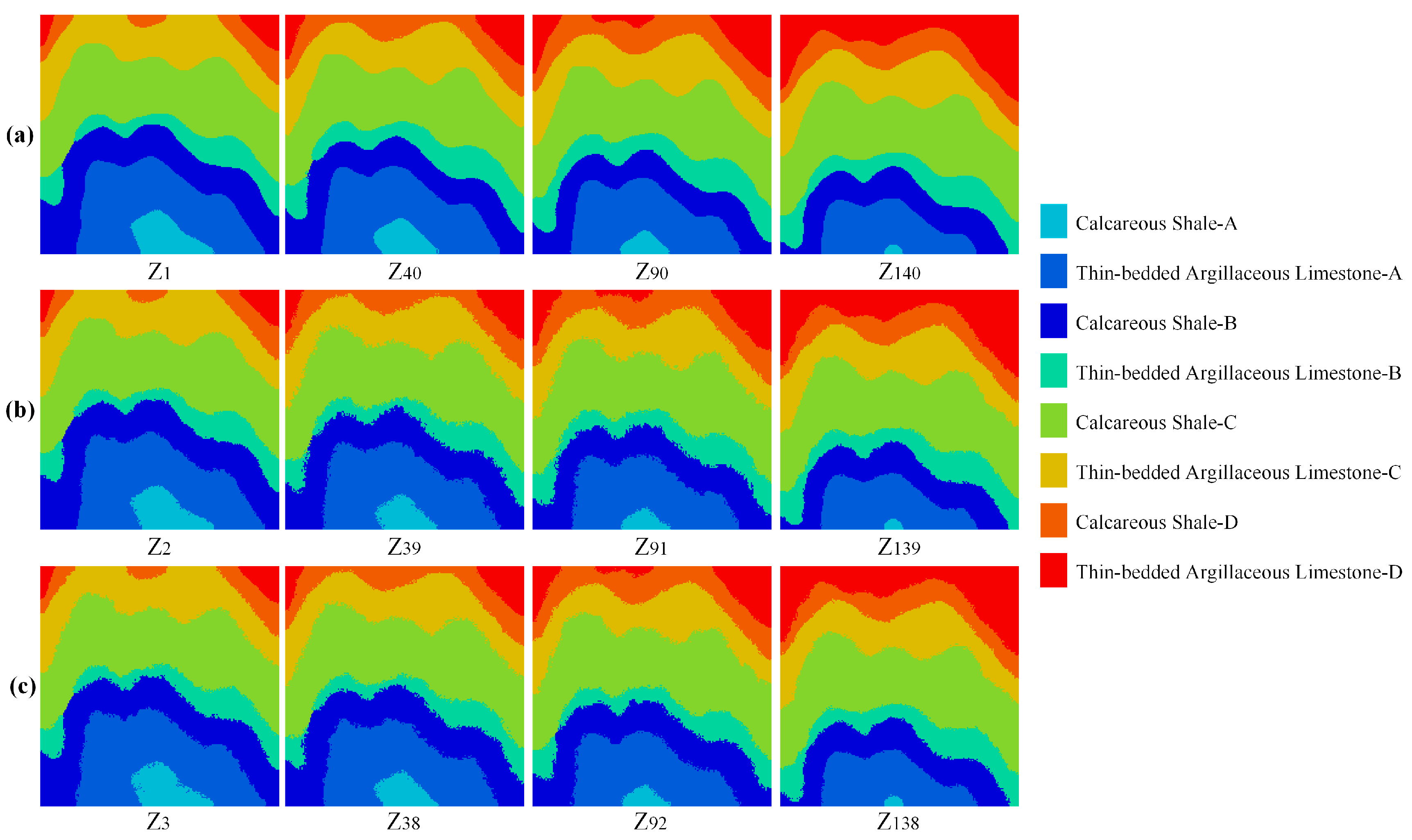
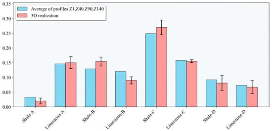
To perform a more detailed assessment of the reconstructed models, quantitative analyses were conducted based on lithofacies variations, connectivity, and variograms. Lithofacies proportion refers to the relative spatial distribution of different lithofacies and represents one of the macroscopic properties of stratigraphy. During structural deformation processes, such as folding, if there is no significant material addition or removal, the overall volumetric proportions of lithofacies within each stratigraphic unit are expected to remain relatively stable. Therefore, the more similar the lithofacies proportions, the smaller the differences between the reconstructed and the conditioning profiles. Figure 16 illustrates the lithofacies distributions across the measured profile (Z1) and three interpreted profiles (Z40, Z90, Z140) and their corresponding reconstructed neighboring profiles.

Figure 16. Comparison of conditional profiles (the measured profile Z1 and three interpreted profiles, Z40, Z90, and Z140) and nearby reconstructed profiles in the 3D model. (a) Four training images. (b) Reconstructed adjacent profiles (separated by one pixel from the training images). (c) (separated by two pixels from the training images).

More specifically, Figure 17 presents a comparison of attribute distributions between the conditional profiles (the measured profile Z1 and three interpreted profiles, Z40, Z90, and Z140) and the 3D reconstructed models. This indicates that the ConvLSTM is capable of accurately constructing 3D fold models while preserving the original attribute proportions without significant deviation.

Figure 17. Comparison of lithofacies proportion variations between the conditional profiles (the measured profile Z1 and three interpreted profiles, Z40, Z90, and Z140) and the reconstructed model profiles.

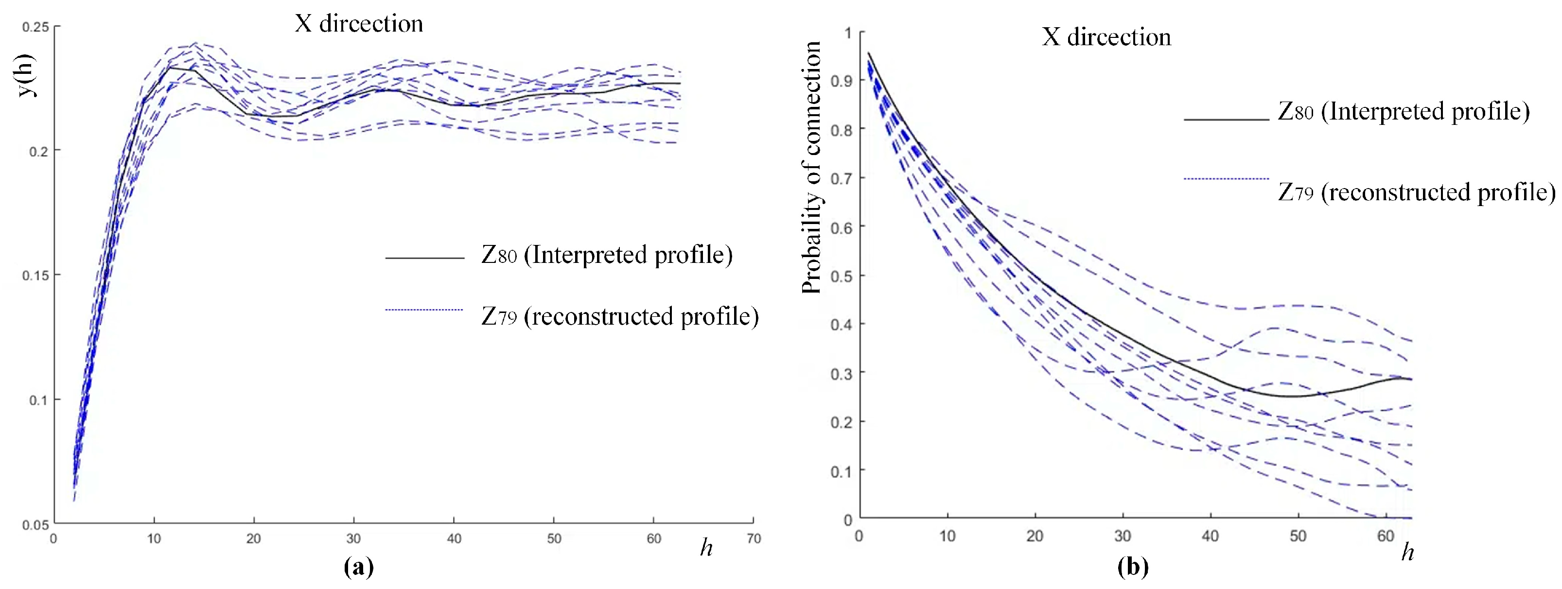
The reconstructed 3D fold models exhibit well-defined stratigraphic sequences, with individual stratigraphic units showing prominent connectivity. Connectivity and variogram analyses were conducted on the ten 3D fold models generated by the LSTM. Using one conditioning profile as a reference, ten neighboring profiles corresponding to each model set were extracted, and their respective connectivity function and variogram curves were plotted. As shown in Figure 18, the characteristic curves of the reconstructed models closely match those of the conditioning profile, indicating that the models accurately reproduce the connectivity and variogram features.

Figure 18. Connectivity and variogram analyses of ConvLSTM-reconstructed models. (a) Analysis of variation of the interpreted profile Z80 and the 10 reconstructed profiles Z79. (b) Connectivity analysis of the interpreted profile Z80 and the 10 reconstructed profiles Z79.

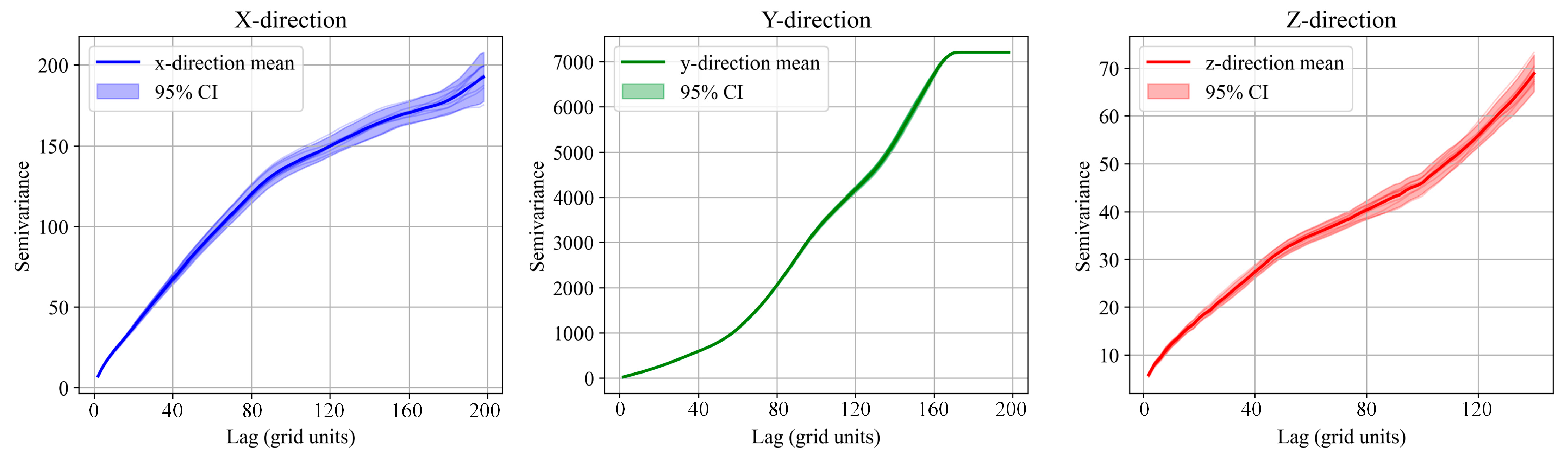
We evaluated the statistical variability among different stochastic realizations by generating ten 3D models and deriving their experimental variograms in the three principal directions. Figure 19 shows that the variogram curves from all ten models are nearly coincident, and the 95% confidence intervals (shaded areas) are extremely tight, suggesting highly consistent spatial statistical characteristics across the models. When combined with the prior analysis of feature differences between slices within the same model, these results demonstrate that our method successfully replicates complex stratigraphic structures and demonstrates outstanding stability.

Figure 19. Variogram analysis of 10 3D models with 95% confidence intervals (CIs).

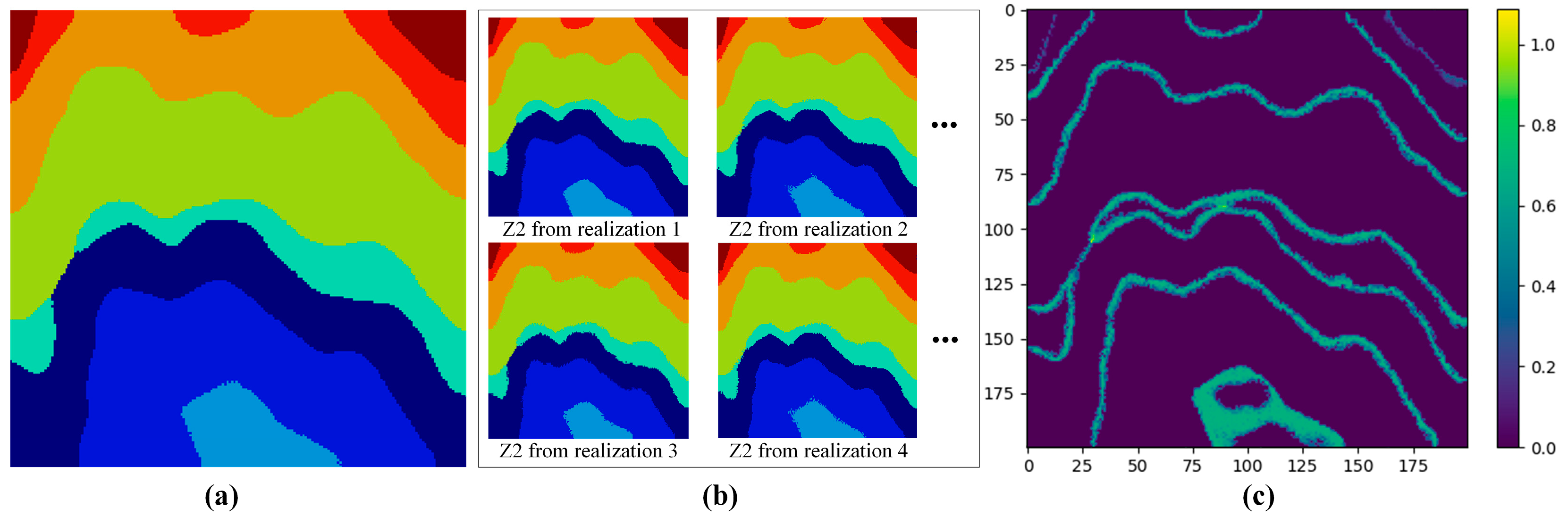
In this study, the measured profile Z1 is used as the reference profile, and the corresponding reconstructed profiles Z2 extracted from ten independent 3D realizations are used to perform the entropy-based uncertainty analysis.

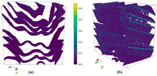
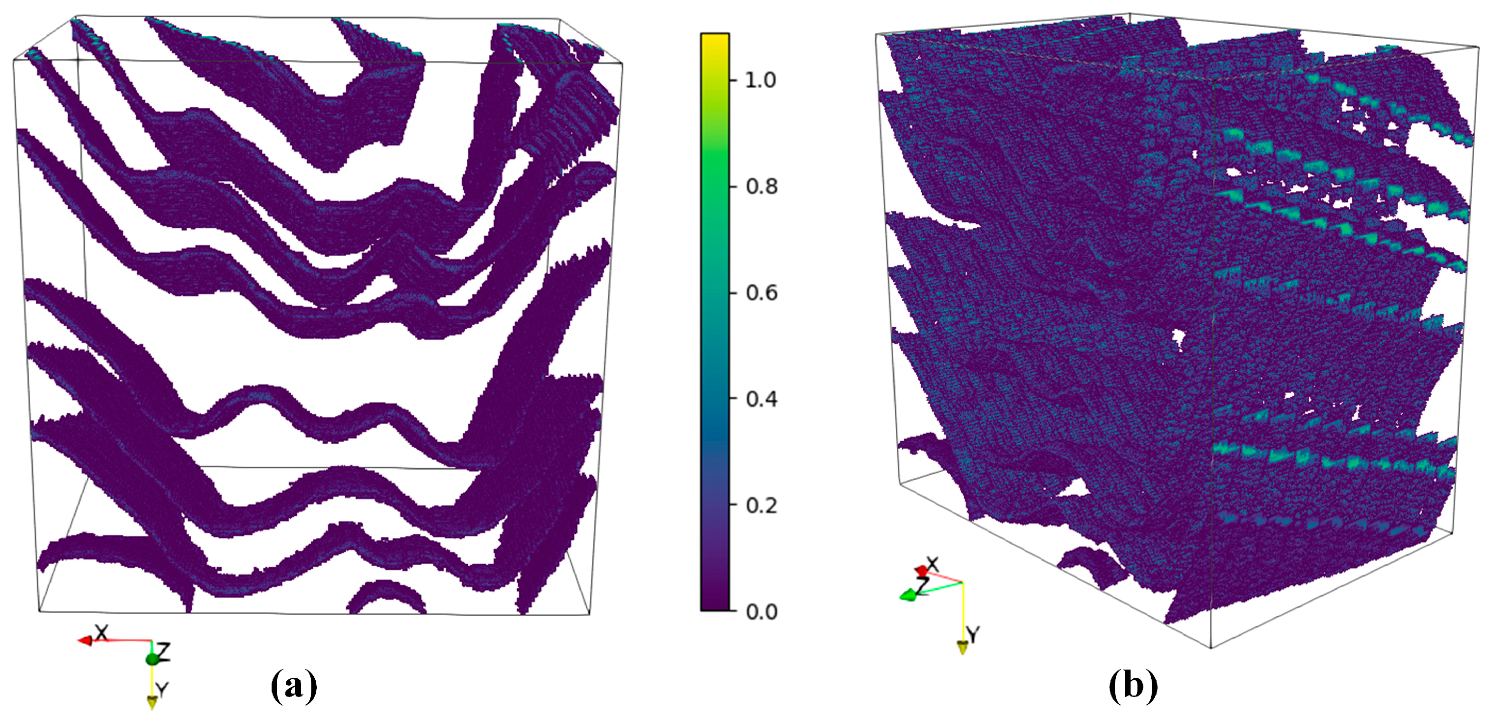
Figure 20 presents the results of the information entropy evaluation. As shown in Figure 20, the reconstructed profiles Z2 exhibit only thin band-shaped uncertain regions near stratigraphic boundaries when compared with the reference profile Z1. As shown in Figure 21, ten sets of 3D models were also generated and used for 3D uncertainty analysis. Similarly to Figure 20, the uncertainty is clustered near the formation interface. The average information entropy value in these uncertain regions remains below 0.5, indicating that the proposed modeling approach maintains a relatively low level of geological uncertainty while preserving the main structural characteristics of the fold system. These results further demonstrate the stability and reliability of the proposed method in reconstructing complex geological structures.

Figure 20. Uncertainty analysis based on information entropy. (a) Reference profile Z1 used as the conditioning profile. (b) Reconstructed profiles Z2 extracted from ten independent 3D realizations. (c) Information entropy map illustrating the spatial distribution of structural uncertainty.

Figure 21. Uncertainty analysis of 10 sets of 3D models based on information entropy. (a,b) show different perspective.

Through the observation and analysis of the reconstructed 3D fold model, the stratigraphic units from Calcareous Shale A to D and Thin-bedded Argillaceous Limestone A to D exhibit continuous spatial distribution and well-defined fold sequences, reflecting complex fold geometries formed by multiphase deformation. The ConvLSTM-based 3D modeling approach effectively preserves interlayer contacts and stratigraphic continuity, accurately reconstructing the fold geometry observed in the original profiles and providing a reliable framework for three-dimensional quantitative analysis of regional polyphase tectonic deformation. The results further demonstrate that the ConvLSTM-based 3D fold modeling method exhibits excellent performance in terms of accuracy. Analyses of lithofacies proportion variations, connectivity, and variograms reveal its remarkable capability in capturing geological structural characteristics, improving modeling efficiency, and enhancing robustness.

4. Discussion

The proposed framework integrates MPS and ConvLSTM networks to address the challenge of reconstructing three-dimensional fold structures from sparse geological sections. The results demonstrate that the method is capable of producing geologically consistent models while maintaining computational efficiency. From a methodological perspective, this approach provides a practical pathway to bridge stochastic simulation and data-driven learning in geological modeling.

Traditional MPS-based approaches are effective in reproducing complex spatial patterns and geological variability, but their computational cost and sensitivity to conditioning data limit their applicability in large-scale or data-intensive scenarios. In contrast, deep learning methods enable efficient prediction once trained, yet their performance strongly depends on the availability and representativeness of training data. By using MPS as a training-data-generation mechanism, the proposed method transforms geological prior knowledge into a form that can be learned by neural networks. This strategy effectively embeds geological constraints into the training process and improves the balance between efficiency and geological realism.

Uncertainty remains an inherent aspect of subsurface modeling, particularly when the available data are sparse and unevenly distributed. The results indicate that the reconstructed models preserve the main structural characteristics of folds, while discrepancies are mainly concentrated near lithological boundaries and transition zones. This behavior reflects the intrinsic ambiguity of geological interfaces and suggests that the model outputs should be interpreted as geologically plausible realizations rather than exact representations of subsurface structures. In this context, the combination of structural similarity measures and entropy-based analysis provides a useful means of assessing the spatial distribution of uncertainty.

The applicability of the proposed method depends on several factors related to both data conditions and geological complexity. The representativeness of the training images plays a critical role, as they define the range of structural patterns that can be learned by the model. In addition, the spatial density and distribution of conditioning sections influence the reliability of the reconstruction, particularly in relation to the characteristic continuity scale of geological structures. When the spacing between sections exceeds this scale, the model tends to exhibit increased uncertainty. The method is therefore more suitable for fold-dominated systems with relatively stable structural patterns, whereas its performance may be reduced in highly complex settings characterized by strong non-stationarity or abrupt structural variations.

The case study further highlights the challenges associated with validation in geological modeling. Due to the limited availability of fully observed subsurface data, part of the reference information is derived from interpretation constrained by borehole data and geological knowledge. As a result, the evaluation focuses on the consistency of reconstructed structures with known geological patterns rather than strict pointwise accuracy. This limitation is common in geological studies and underscores the importance of interpreting modeling results within a broader geological context.

Another aspect worth noting is the influence of grid resolution on model representation. The relatively coarse discretization adopted in this study is consistent with the scale and quality of the available data and allows for efficient model training and prediction. Although higher-resolution grids may improve visual smoothness and capture finer-scale features, increasing resolution without additional constraints may introduce artificial details that are not supported by observations. Therefore, the current framework prioritizes the reproduction of large-scale structural characteristics over fine-scale geometric refinement.

Despite its advantages, the proposed method has several limitations. Its performance depends on the quality and diversity of the training dataset, and its ability to represent highly complex geological scenarios remains constrained. In addition, the current framework does not explicitly incorporate physical or mechanical constraints, which may be important for certain applications. Future work will focus on integrating multi-source geological data, extending the method to more complex structural settings, and improving uncertainty quantification at the three-dimensional scale.

5. Conclusions

This study proposes a three-dimensional geological modeling framework that integrates sectional constraints with training-image-based spatial simulation to improve structural consistency in section-based geological reconstruction. The main contributions of this work can be summarized as follows:

(1)

A hybrid reconstruction workflow was developed to combine geological profile constraints with training-image-driven spatial inference, enabling the generation of geologically consistent three-dimensional models from limited sectional information.

(2)

The proposed framework improves structural continuity between adjacent profiles and effectively reduces mismatch artifacts commonly observed in interpolation-based reconstruction approaches.

(3)

Benchmark experiments and the Nepal fold case study demonstrate that the method achieves low volumetric reconstruction error while preserving realistic facies connectivity and stratigraphic structure.

(4)

The study highlights the importance of training image representativeness and sectional data density for ensuring reliable reconstruction.

Overall, the proposed approach provides an effective and computationally feasible solution for reconstructing moderately complex geological architectures from limited profile observations. The framework offers a balance between geological realism and statistical consistency, and it provides a practical tool for geological modeling applications where direct three-dimensional observations are sparse.

References

- Li, H.; Wan, B.; Chu, D.; Wang, R.; Ma, G.; Fu, J.; Xiao, Z. Progressive geological modeling and uncertainty analysis using machine learning. ISPRS Int. J. Geo-Inf. 2023, 12, 97. [Google Scholar] [CrossRef] [Scilit]
- Liu, L.; Li, T.; Ma, C. Research on 3D geological modeling method based on deep neural networks for drilling data. Appl. Sci. 2024, 14, 423. [Google Scholar] [CrossRef] [Scilit]
- Hong, J.; Oh, S. Model selection for mineral resource assessment considering geological and grade uncertainties, Application of multiple-point geostatistics and a cluster analysis to an iron deposit. Nat. Resour. Res. 2021, 30, 2047–2065. [Google Scholar] [CrossRef] [Scilit]
- Enemark, T.; Madsen, R.B.; Sonnenborg, T.O.; Andersen, L.T.; Sandersen, P.B.E.; Kidmose, J.; Møller, I.; Hansen, T.M.; Jensen, K.H.; Høyer, A.-S. Incorporating interpretation uncertainties from deterministic 3D hydrostratigraphic models in groundwater models. Hydrol. Earth Syst. Sci. 2024, 28, 505–523. [Google Scholar] [CrossRef] [Scilit]
- Li, X.; Yuan, F.; Zhang, M.; Jowitt, S.M.; Ord, A.; Zhou, T.; Dai, W. 3D computational simulation-based mineral prospectivity modeling for exploration for concealed Fe–Cu skarn-type mineralization within the Yueshan orefield, Anqing district, Anhui Province, China. Ore Geol. Rev. 2019, 105, 1–17. [Google Scholar] [CrossRef] [Scilit]
- Zou, L.; Hakansson, U.; Cvetkovic, V. Cement grout propagation in two-dimensional fracture networks, Impact of structure and hydraulic variability. Int. J. Rock Mech. Min. Sci. 2019, 115, 1–10. [Google Scholar] [CrossRef] [Scilit]
- Liu, G.; Fang, H.; Chen, Q.; Cui, Z.; Zeng, M. A feature-enhanced MPS approach to reconstruct 3D deposit models using 2D geological cross sections, A case study in the Luodang Cu deposit, Southwestern China. Nat. Resour. Res. 2022, 31, 3101–3120. [Google Scholar] [CrossRef] [Scilit]
- Gong, W.; Zhao, C.; Juang, C.H.; Tang, H.; Wang, H.; Hu, X. Stratigraphic uncertainty modelling with random field approach. Comput. Geotech. 2020, 125, 103681. [Google Scholar] [CrossRef] [Scilit]
- Guo, J.; Wang, Z.; Li, C.; Li, F.; Jessell, M.W.; Wu, L.; Wang, J. Multiple-point geostatistics-based 3D automatic geological modeling and uncertainty analysis for borehole data. Nat. Resour. Res. 2022, 31, 2347–2367. [Google Scholar] [CrossRef] [Scilit]
- Wei, X.; Wang, H. Stochastic stratigraphic modeling using Bayesian machine learning. Eng. Geol. 2022, 307, 106789. [Google Scholar] [CrossRef] [Scilit]
- Wu, X.; Liu, G.; Weng, Z.; Tian, Y.; Zhang, Z.; Li, Y.; Chen, G. Constructing 3D geological models based on large-scale geological maps. Open Geosci. 2021, 13, 851–866. [Google Scholar] [CrossRef] [Scilit]
- Gravey, M.; Mariethoz, G. QuickSampling v1.0: A robust and simplified pixel-based multiple-point simulation approach. Geosci. Model Dev. 2020, 13, 2611–2630. [Google Scholar] [CrossRef] [Scilit]
- He, H.; Xiao, J.; He, J.; Wei, B.; Ma, X.; Huang, F.; Cai, X.; Zhou, Y.; Bi, J.; Zhao, Y.; et al. Three-dimensional geological modeling of the shallow subsurface and its application: A case study in Tongzhou District, Beijing, China. Appl. Sci. 2023, 13, 1932. [Google Scholar] [CrossRef] [Scilit]
- Mohammed, M.A.; Mohammed, S.H.; Szabó, N.P.; Szűcs, P. Geospatial modeling for groundwater potential zoning using a multi-parameter analytical hierarchy process supported by geophysical data. Discov. Appl. Sci. 2024, 6, 121. [Google Scholar] [CrossRef] [Scilit]
- Comunian, A.; Jha, S.K.; Giambastiani, B.M.; Mariethoz, G.; Kelly, B.F.J. Training Images from Process-Imitating Methods, An Application to the Lower Namoi Aquifer, Murray-Darling Basin, Australia. Math. Geosci. 2014, 46, 241–260. [Google Scholar] [CrossRef] [Scilit]
- Ke, L.; Ruan, F.; Duan, T.; Li, Z.; Wang, X.; Zhao, L. Integrated Geomodel Accuracy Enhancement Based on Embedded MPS Geological Modeling for Thin Interbedded Reservoirs. Energies 2023, 16, 6850. [Google Scholar] [CrossRef] [Scilit]
- Bian, X.; Fan, Z.; Liu, J.; Li, X.; Zhao, P. Regional 3D geological modeling along metro lines based on stacking ensemble model. Undergr. Space 2024, 18, 65–82. [Google Scholar] [CrossRef] [Scilit]
- Lyu, B.; Wang, Y.; Shi, C. Multi-scale generative adversarial networks (GAN) for generation of 3D subsurface geological models from limited boreholes and prior geological knowledge. Comput. Geotech. 2024, 170, 106336. [Google Scholar] [CrossRef] [Scilit]
- Shi, C.; Wang, Y.; Yang, H. An ensemble learning paradigm for subsurface stratigraphy from sparse measurements and augmented training images. Tunn. Undergr. Space Technol. 2024, 153, 105972. [Google Scholar] [CrossRef] [Scilit]
- Ayad, A.; Bakkali, S. Multifractal Classification of the Disturbed areas of the Sidi Chennane Phosphate Deposit. Econ. Environ. Geol. 2022, 55, 231–239. [Google Scholar] [CrossRef] [Scilit]
- Ayad, A.; Bakkali, S. Using the mass-radius method to quantify the disturbed zones in Sidi Chennane mine through geo-electrical images. Int. J. Min. Geo-Eng. 2022, 56, 225–230. [Google Scholar] [CrossRef]
- Fan, W.; Azevedo, L.; Liu, G.; Chen, Q.; Wu, X.; Li, Y. Automatic reconstruction of 3D geological models based on Recurrent Neural Network and predictive learning. Comput. Geosci. 2025, 204, 105996. [Google Scholar] [CrossRef] [Scilit]
- Sun, H.; Sheng, L.; Dai, Y.; Li, X.; Rui, Y.; Lu, L. 3D geological modeling of tunnel alignment in the complex mountainous region of Yongshan, China, based on multisource data fusion. Eng. Geol. 2025, 354, 108209. [Google Scholar] [CrossRef] [Scilit]
- Liu, Q.; Liu, R.; He, T.; Zhang, H. Prediction of Lithofacies and 3D Geological Modeling Based on CNN-LSTM Spatiotemporal Networks. Math. Geosci. 2025, 57, 1357–1377. [Google Scholar] [CrossRef] [Scilit]
- Al-Selwi, S.M.; Hassan, M.F.; Abdulkadir, S.J.; Muneer, A.; Sumiea, E.H.; Alqushaibi, A.; Ragab, M.G. RNN-LSTM: From applications to modeling techniques and beyond—Systematic review. J. King Saud Univ.-Comput. Inf. Sci. 2024, 36, 102068. [Google Scholar] [CrossRef] [Scilit]
- Wen, X.; Li, W. Time series prediction based on LSTM-attention-LSTM model. IEEE Access 2023, 11, 48322–48331. [Google Scholar] [CrossRef] [Scilit]
- Mariethoz, G.; Renard, P.; Straubhaar, J. The direct sampling method to perform multiple-point geostatistical simulations. Water Resour. Res. 2010, 46, W11536. [Google Scholar] [CrossRef] [Scilit]
- Straubhaar, J.; Renard, P. Conditioning multiple-point statistics simulation to inequality data. Earth Space Sci. 2021, 8, e2020EA001515. [Google Scholar] [CrossRef] [Scilit]
- Dagasan, Y.; Juda, P.; Renard, P. Using generative adversarial networks as a fast forward operator for hydrogeological inverse problems. Groundwater 2020, 58, 938–950. [Google Scholar] [CrossRef] [Scilit]
- Bengio, Y.; Simard, P.; Frasconi, P. Learning long-term dependencies with gradient descent is difficult. IEEE Trans. Neural Netw. 1994, 5, 157–166. [Google Scholar] [CrossRef] [Scilit] [PubMed]
- Hochreiter, S.; Schmidhuber, J. Long short-term memory. Neural Comput. 1997, 9, 1735–1780. [Google Scholar] [CrossRef] [Scilit] [PubMed]
Disclaimer/Publisher’s Note: The statements, opinions and data contained in all publications are solely those of the individual author(s) and contributor(s) and not of MDPI and/or the editor(s). MDPI and/or the editor(s) disclaim responsibility for any injury to people or property resulting from any ideas, methods, instructions or products referred to in the content. |
© 2026 by the authors. Licensee MDPI, Basel, Switzerland. This article is an open access article distributed under the terms and conditions of the Creative Commons Attribution (CC BY) license.