


Abstract
Accurate brain tumor segmentation in magnetic resonance imaging (MRI) is essential for diagnosis, treatment planning, and therapy monitoring. Conventional deep learning models often struggle with large variations in tumor shape, size, and contrast, as well as severe foreground–background imbalance. To address these challenges, this study presents Deep-MiSR, an enhanced encoder–decoder framework built upon DeepLabV3+ with a MobileNetV2 backbone, tailored for single-modality contrast-enhanced T1-weighted (T1CE) MRI segmentation. Three complementary components are integrated into the architecture: mixed depthwise convolution (MixConv) with heterogeneous kernels within the atrous spatial pyramid pooling module for multi-scale feature aggregation, a squeeze-and-excitation block for adaptive channel recalibration, and R-Drop regularization that enforces prediction consistency via symmetric Kullback–Leibler divergence. The model was evaluated on 3064 T1CE slices from 233 patients drawn from the publicly available Nanfang Hospital brain MRI dataset. Deep-MiSR achieved a Dice similarity coefficient of 0.9281, a mean intersection-over-union of 0.8738, a precision of 0.8839, and a 95th-percentile Hausdorff distance of 7.69 mm, demonstrating consistent improvements over both the DeepLabV3+ baseline and all prior methods evaluated on the same data. Ablation studies confirmed that each component contributes independently, with R-Drop providing the largest individual gain. These findings demonstrate that combining multi-scale convolution, channel attention, and consistency regularization constitutes an effective and computationally practical strategy for robust single-modality brain tumor segmentation.
1. Introduction
Recent GLOBOCAN 2022 estimates reveal that brain and central nervous system (CNS) tumors accounted for 321,624 new cases and 248,403 deaths worldwide in 2022 [1]. Among these, gliomas, particularly glioblastoma (WHO grade IV), represent the most aggressive primary malignant brain tumors in adults, with median survival of 12–15 months despite maximal surgical resection, radiotherapy, and chemotherapy [2,3]. Precise magnetic resonance imaging (MRI)-based tumor boundary delineation is essential for diagnosis, surgical planning, radiotherapy contouring, and longitudinal response assessment, as resection extent remains a key prognostic factor [4,5].
Multi-parametric MRI (T1-weighted, T1-weighted contrast-enhanced (T1CE), T2-weighted, fluid-attenuated inversion recovery (FLAIR) sequences) offers superior soft-tissue contrast and is the preferred modality for non-invasive brain tumor assessment [6]. However, manual segmentation by expert neuroradiologists is time consuming, labor intensive, and prone to inter-observer variability, with reported human inter-rater Dice scores around 0.74 [7]. These limitations substantially hinder scalability in routine clinical workflows and have motivated extensive research into automated brain tumor segmentation methods. Although multimodal and three-dimensional MRI pipelines dominate contemporary benchmarks such as BraTS, their translation to routine clinical workflows remains constrained by acquisition variability and computational requirements [7,8]. In real-world practice, contrast-enhanced T1-weighted (T1CE) imaging is among the most consistently available sequences, while additional modalities may be missing or misaligned due to protocol differences and patient motion. Moreover, 3D models typically incur substantially higher memory and latency costs, limiting feasibility on standard clinical workstations. Consequently, efficient 2D segmentation methods tailored to single-modality MRI remain clinically relevant, particularly in resource-constrained settings. It is acknowledged, however, that T1CE imaging captures primarily the contrast-enhancing tumor core and may not fully delineate infiltrative margins visible on T2 or FLAIR sequences [9]; this represents an inherent scope limitation of single-modality approaches that is discussed further in Section 5.3.
In semantic segmentation, the goal is to assign a class label to every pixel of an input image; encoder–decoder networks, which progressively compress spatial information into high-level representations and recover spatial detail through upsampling, have become the dominant paradigm for this task in medical imaging [10]. Deep learning, particularly convolutional neural networks (CNNs), has transformed medical image segmentation. The U-Net architecture [11] and its variants became foundational for brain tumor segmentation through the BraTS challenge series (2012–present) [7]. Since 2020, nnU-Net has dominated leaderboards, achieving Dice scores > 0.90 across tumor sub-regions (enhancing tumor, edema, necrosis) on multimodal MRI [12]. Recent BraTS challenges (2021–2024) further improved performance to 0.90–0.94 Dice via nnU-Net ensembles, vision transformers (UNETR [13], Swin-UNETR [14]), and test-time augmentation [15].
Despite these advances, clinical adoption remains challenging. Transformer-based models demand substantial computational resources, extensive pre-training, and >40 GB GPU memory, exceeding standard hospital workstations (8–16 GB), while requiring hours of inference [8]. Conversely, lightweight CNNs struggle with irregular/small glioma lesions, particularly low-contrast tumors comprising <1% of pixels, causing under-segmentation due to severe foreground–background imbalance [16]. Hybrid efficiency-focused CNN enhancements thus represent a critical research direction [15].
DeepLabV3+, originally designed for natural scene segmentation [17], has gained significant traction in medical imaging through its efficient encoder–decoder design, atrous convolutions, and atrous spatial pyramid pooling (ASPP) module enabling multi-scale context aggregation with minimal computational overhead [18,19]. However, standard implementations face limitations on heterogeneous glioma datasets: fixed-kernel depthwise convolutions restrict receptive field diversity; ASPP lacks channel recalibration, underemphasizing tumor features; and training omits consistency regularization, compromising stability on small, imbalanced data. Large-scale evaluations of brain tumor segmentation benchmarks have shown that improvements in segmentation accuracy are often driven not solely by architectural complexity, but by disciplined training strategies, inductive biases, and targeted architectural refinements aligned with the data characteristics and evaluation protocol [7,12]. In particular, well-trained U-Net-style convolutional architectures remain strong baselines and are frequently difficult to surpass, even when compared against substantially more complex designs. These observations suggest that practical performance gains can be achieved by enhancing established CNN pipelines through lightweight, complementary components that improve multi-scale representation, feature selectivity, and prediction stability, without incurring excessive computational cost.
To address these limitations while maintaining a moderate computational footprint, we introduce Deep-MiSR, an enhanced DeepLabV3+ architecture tailored for 2D brain tumor segmentation on T1CE MRI. The model integrates three complementary components—heterogeneous-kernel mixed depthwise convolution (MixConv) within the ASPP module, a squeeze-and-excitation (SE) block for post-ASPP channel recalibration, and logit-level R-Drop regularization (regularized dropout) to strengthen multi-scale representation, channel selectivity, and training stability. All modules are implemented directly within the DeepLabV3+ pipeline used in our experiments. We evaluate the proposed model on 3064 contrast-enhanced T1-weighted MRI slices from 233 patients with meningioma, glioma, and pituitary tumors, using a fixed random slice-wise split into training and validation sets (80%/20%). The validation set is used for model selection and for reporting slice-level performance under this protocol. Deep-MiSR achieves a Dice coefficient of 0.9281 and a mean intersection over union (mIoU) of 0.8738. Ablation studies show that MixConv, SE block, and R-Drop each provide independent improvements, while their combination yields the most robust performance. Under identical training conditions, the proposed model demonstrates superior mIoU performance compared to U-Net variants, SegNet, and TransUNet, offering clearer boundary delineation and improved segmentation reliability. These findings highlight the practical benefits of targeted multi-scale enhancement, adaptive channel weighting, and prediction-consistency regularization for medical image segmentation.
The main contributions of this study are as follows:
- Multi-scale enhancement within ASPP via heterogeneous-kernel MixConv. We integrate mixed depthwise convolution with heterogeneous kernel sizes (, , ) into the ASPP module to enrich multi-scale contextual representation, improving sensitivity to heterogeneous tumor morphology and boundary precision.
- Adaptive channel recalibration using a post-ASPP SE block. A squeeze-and-excitation (SE) block is applied immediately after ASPP to adaptively reweight channel responses, enhancing tumor-relevant feature representation and complementing the multi-scale information produced by MixConv.
- Prediction-consistency regularization with R-Drop and systematic empirical validation. We employ logit-level R-Drop regularization with symmetric Kullback–Leibler divergence to improve training stability and prediction consistency on imbalanced T1CE data. Comprehensive ablation studies quantify the individual and combined effects of MixConv, SE, and R-Drop, demonstrating consistent improvements over multiple CNN- and transformer-based baselines under identical experimental conditions.
- Effective single-modality T1CE brain tumor segmentation. We demonstrate that targeted architectural and training-level refinements to DeepLabV3+ enable high-performance brain tumor segmentation using only contrast-enhanced T1-weighted (T1CE) MRI, achieving a Dice coefficient of 0.9281 without reliance on multimodal inputs or 3D processing.
Taken together, these contributions demonstrate that targeted architectural refinements, heterogeneous multi-scale filtering, adaptive channel recalibration, and prediction-consistency regularization can substantially enhance segmentation quality on single-modality T1CE MRI without requiring complex backbones or multimodal inputs. The proposed design focuses on improving representation where conventional CNN-based models encounter difficulty, particularly for heterogeneous glioma morphology and low-contrast tumor margins.
The remainder of the paper is organized as follows. Section 2 reviews related work on deep-learning-based tumor segmentation. Section 3 describes the dataset, preprocessing pipeline, model architecture, and training procedures. Section 4 reports quantitative and qualitative results, including ablation studies and boundary-based evaluations. Section 5 discusses the implications of these findings and outlines the limitations. Section 6 concludes the study and highlights directions for future research.
2. Related Work
CNN-based architectures have dominated brain tumor segmentation since U-Net [11] established the encoder–decoder paradigm with skip connections via BraTS [7]. Subsequent advances incorporated deeper backbones [20], residual connections [21], and self-configuring frameworks. nnU-Net [12] has led BraTS leaderboards since 2020 through automated adaptation. Recent comprehensive reviews highlight U-Net enhancements with transfer learning [22] and evolution toward hybrid CNN–transformer models achieving Dice [23,24], though computational demands persist as a key challenge.
Beyond the multimodal BraTS benchmark, the public Nanfang T1CE dataset has gained prominence in single-modality brain tumor research; however, most studies address tumor classification rather than pixel-wise segmentation [25,26,27,28]. In contrast, fewer efforts pursue semantic segmentation [29,30,31,32]. For instance, Badža et al. [32] developed a compact convolutional autoencoder on 3064 T1CE slices from 233 patients, reporting pixel accuracy of 99.28% alongside a mean Dice of 0.7287, highlighting the limitations of accuracy metrics in imbalanced settings. Similarly, Gupta et al. [31] applied a recurrent-residual CNN to the same dataset, achieving an F1 score of 0.8495 and IoU of 0.8665, which improved overlap-based performance over U-Net variants while underscoring inconsistent benchmark reporting for Nanfang pixel-wise segmentation.
DeepLabV3+ [17], featuring atrous convolutions and the atrous spatial pyramid pooling (ASPP) module, has emerged as a competitive alternative to U-Net variants in medical imaging by efficiently capturing multi-scale contextual information. Several studies have adapted DeepLabV3+ for brain tumor segmentation [33,34]. However, its standard implementation reveals architectural constraints pertinent to heterogeneous glioma datasets on single-modality T1CE: depthwise convolutions employ fixed kernel sizes per channel, restricting receptive field diversity [35]; the ASPP module lacks channel-wise recalibration to enhance feature selectivity in tumor regions [36]; and it incorporates no consistency regularization to improve generalization on imbalanced data [37]. These limitations necessitate targeted refinements to ASPP for enhanced boundary accuracy and robustness.
Transformer-based architectures have further advanced tumor segmentation by leveraging self-attention for long-range dependency modeling. UNETR [13] and Swin-UNETR [14] replace traditional convolutional encoders with transformer-based modules, achieving strong performance on multimodal BraTS benchmarks. Hybrid CNN–Transformer designs have also been proposed specifically for brain tumor segmentation; BiTr-UNet [38] combines convolutional encoders with transformer blocks to enhance global context modeling on multimodal MRI. While these models achieve competitive Dice scores across tumor subregions, they typically require substantially increased computational resources and memory consumption [39,40], which limits their practical deployment in many clinical environments.
2.1. Multi-Scale Feature Extraction
Accurate segmentation of tumors exhibiting diverse sizes and morphologies necessitates robust multi-scale feature representations. Traditional approaches employ pyramid pooling or dilated convolutions with fixed atrous rates, whereas recent studies explore heterogeneous kernels or explicit multi-scale fusion modules. Xiong et al. [29] proposed YOLO-BT, a multi-scale feature fusion framework integrating BiFPN and deformable large-kernel attention for single-modality brain tumor segmentation on the Nanfang T1CE dataset. Their model achieved notable performance (mIoU = 0.863, Dice = 0.926), significantly surpassing conventional CNN baselines including U-Net and DeepLabV3+. Nonetheless, its detection-oriented backbone introduces architectural complexity, motivating the development of streamlined segmentation-specific CNN designs. Complementing this, Tiwary et al. [30] utilized an EfficientNet-enhanced U-Net, improving multi-scale representation through compound scaling of depth, width, and resolution. Evaluated on the same dataset, the method attained high class-wise Dice scores (0.964 for meningioma, 0.832 for glioma, and 0.944 for pituitary), demonstrating the efficacy of enhanced multi-scale encoding even in single-modality contexts. However, its lack of overall Dice or IoU metrics and class-specific formulation restricts direct comparison with pixel-wise segmentation frameworks.
2.2. Attention and Channel Recalibration Mechanisms
Attention mechanisms have been widely employed to emphasize tumor-relevant features in brain MRI segmentation. He et al. [41] proposed a hybrid U-Net model integrating attention modules to focus on salient regions adaptively. Channel-attention designs such as CAGs-Net [42] have further improved segmentation by jointly refining spatial and channel responses, achieving superior Dice scores. Squeeze-and-excitation (SE) blocks [36], as lightweight channel-wise recalibration modules, have been extensively surveyed and have been shown to enhance feature selectivity in challenging tumor regions. For models like DeepLabV3+, attention has predominantly been introduced as add-on modules [34], while systematic integration of SE-style recalibration directly within the ASPP module, combined with regularization, remains comparatively underexplored.
2.3. Regularization and Consistency Training
Class imbalance and limited annotated data pose significant challenges leading to overfitting in brain tumor segmentation models. Various dropout variants and consistency regularization techniques on unlabeled or augmented samples have demonstrated improvements in model generalization [43,44]. Among these, R-Drop [37], which enforces symmetric Kullback–Leibler divergence loss between stochastic forward passes of the same network, has recently emerged as particularly effective in medical imaging contexts, offering more robust regularization than traditional dropout without requiring additional data augmentation.
2.4. Research Gap
Although multi-scale convolution, channel attention, and consistency-based regularization have been explored in medical image segmentation, these components are typically studied independently or applied within U-Net-derived architectures. For DeepLabV3+-based models, most prior improvements focus on adjusting atrous rates, adding ASPP branches, or designing ensemble structures, with limited exploration of heterogeneous-kernel convolutions or channel recalibration within the ASPP pathway. Similarly, R-Drop regularization has rarely been applied to stabilize pixel-wise segmentation, particularly under limited annotation conditions. To the best of our knowledge, no existing work has integrated MixConv within ASPP, SE-based channel recalibration after ASPP, and logit-level R-Drop regularization into a unified DeepLabV3+ framework for single-modality T1CE brain tumor segmentation.
To address these gaps, this study evaluates the combined impact of MixConv, SE attention, and R-Drop regularization within a DeepLabV3+ architecture. The proposed model is compared against U-Net and Transformer-based baselines on the Nanfang dataset to examine whether these design refinements improve segmentation accuracy and boundary delineation for single-modality T1CE MRI.
3. Materials and Methods
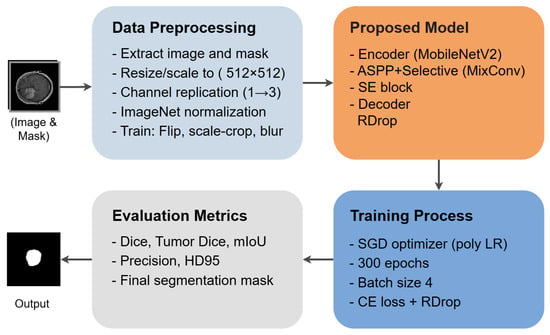
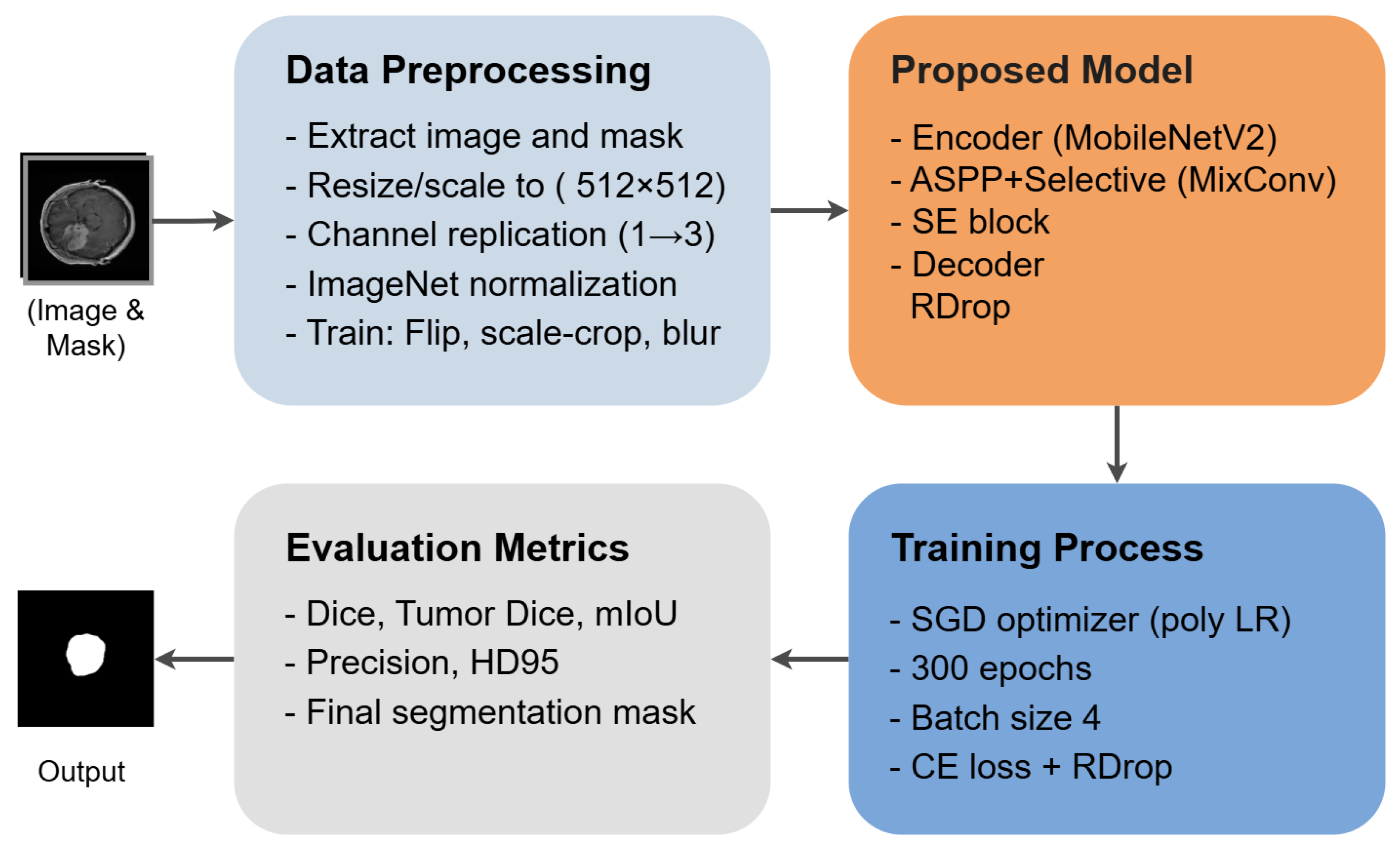
This section details the dataset, preprocessing pipeline, proposed Deep-MiSR architecture, training protocol, and evaluation metrics employed in this study. An overview of the end-to-end methodology is shown in Figure 1.
Figure 1.
Overview of the proposed methodology: data acquisition and preprocessing, Deep-MiSR architecture, and evaluation pipeline.
3.1. Dataset and Data Preprocessing
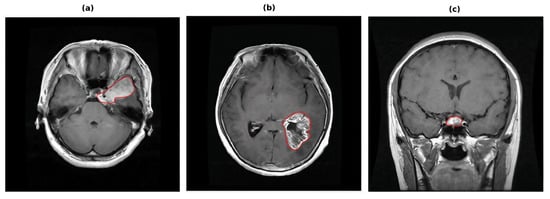
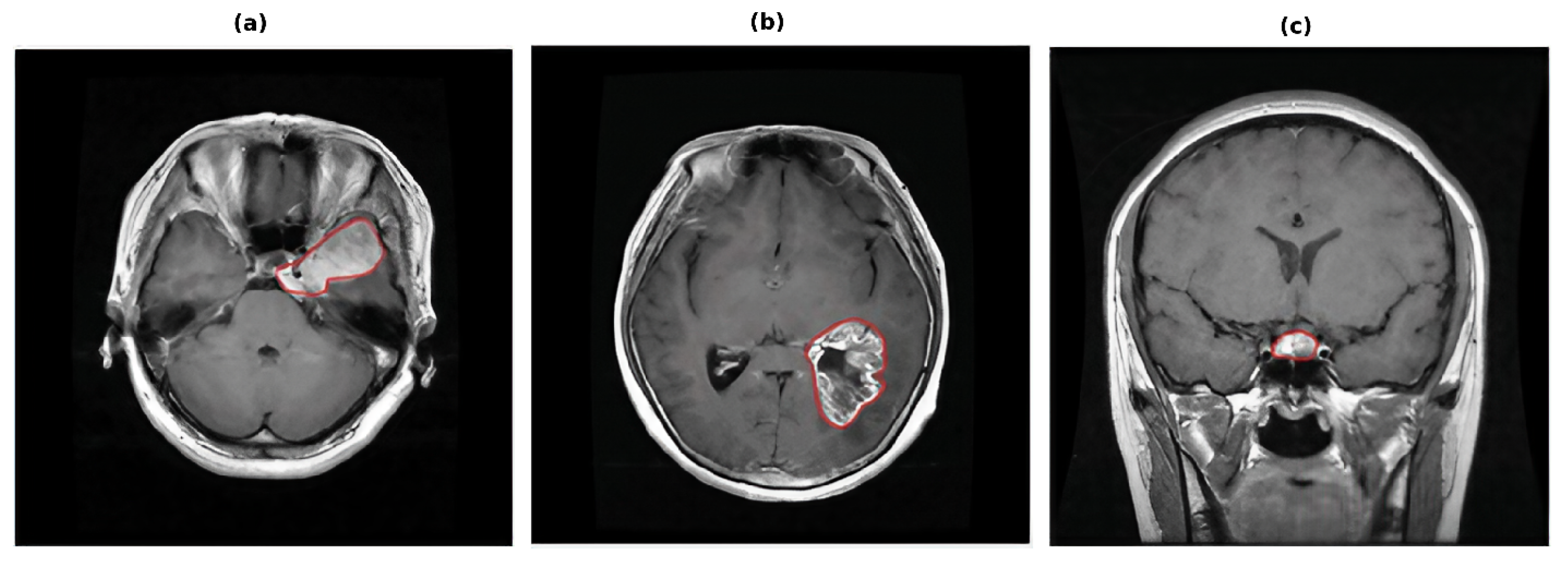
Dataset. We evaluate on the publicly available brain tumor MRI dataset collected at Nanfang Hospital, Southern Medical University, Guangzhou, China, between 2005 and 2010 [45]. The dataset comprises 3064 T1-weighted contrast-enhanced (T1CE) axial slices from 233 patients diagnosed with one of three tumour types: meningioma (708 slices), glioma (1426 slices), and pituitary tumour (930 slices). Representative samples from each class are shown in Figure 2.
Figure 2.
Sample T1CE slices and corresponding ground-truth masks for each tumour type: meningioma (a), glioma (b), and pituitary tumour (c).
The dataset is partitioned slice-wise into 2451 training images (80%) and 613 validation images (20%) using a fixed random split. All experiments share the same split files to ensure fair comparison across model variants. Tumor type labels in the Cheng et al. [45]. dataset were assigned at the originating clinical institution; however, the specific diagnostic confirmation method for individual cases is not reported in the publicly available dataset documentation.
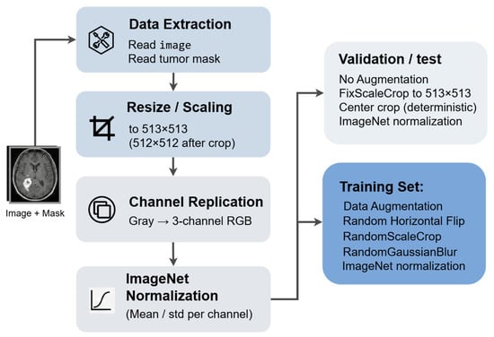
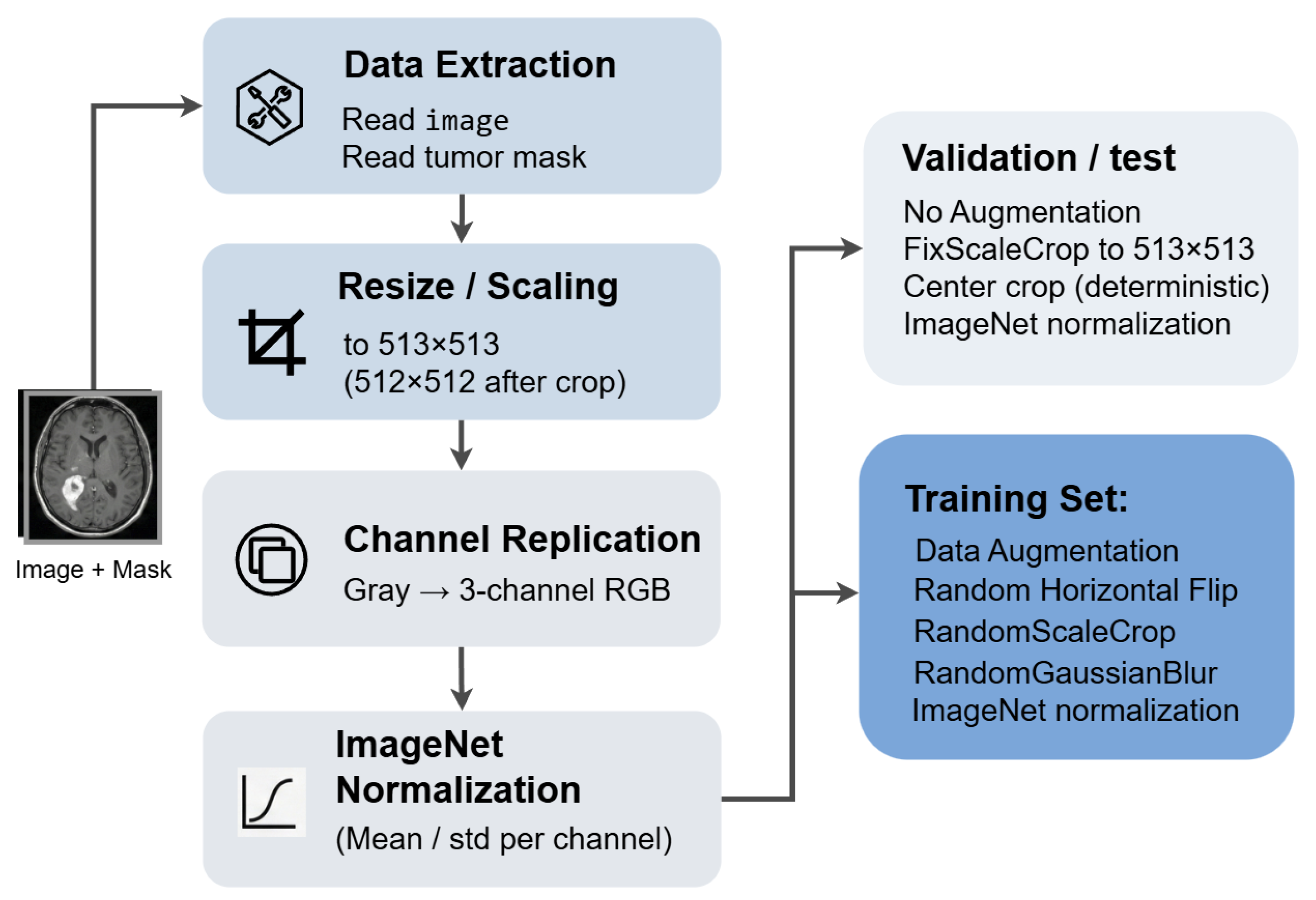
Preprocessing. The original (.mat) files from the Cheng et al. [45] dataset are converted to PNG format offline. Each resulting image is pixels and stores grayscale intensity values in a four-channel (RGBA) representation with identical R, G, and B channels. At loading time, the dataloader converts each image to three-channel RGB via PIL’s convert(‘RGB’), producing three identical channels suitable for ImageNet-pretrained backbones. Ground-truth masks are loaded as binary images via convert(‘1’) and stored with a _mask suffix. The preprocessing pipeline is illustrated in Figure 3.
Figure 3.
Data preprocessing pipeline: .mat to PNG conversion, three-channel RGB conversion, augmentation, normalization, and tensor conversion.
Data augmentation. During training, the following augmentations are applied sequentially:
- Random horizontal flip with probability .
- Random scale and crop: the shorter edge is randomly resized to an integer in , followed by a random crop.
- Random Gaussian blur with probability and a random radius .
- Normalization with ImageNet channel means and standard deviations .
During validation, augmentation is replaced by a deterministic fixed-scale centre crop: the image is resized so that its shorter edge equals 513 pixels, then centre-cropped to and normalized with the same ImageNet statistics. This deterministic pipeline ensures reproducible evaluation.
3.2. Baseline Model: DeepLabV3+
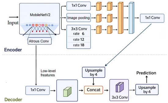
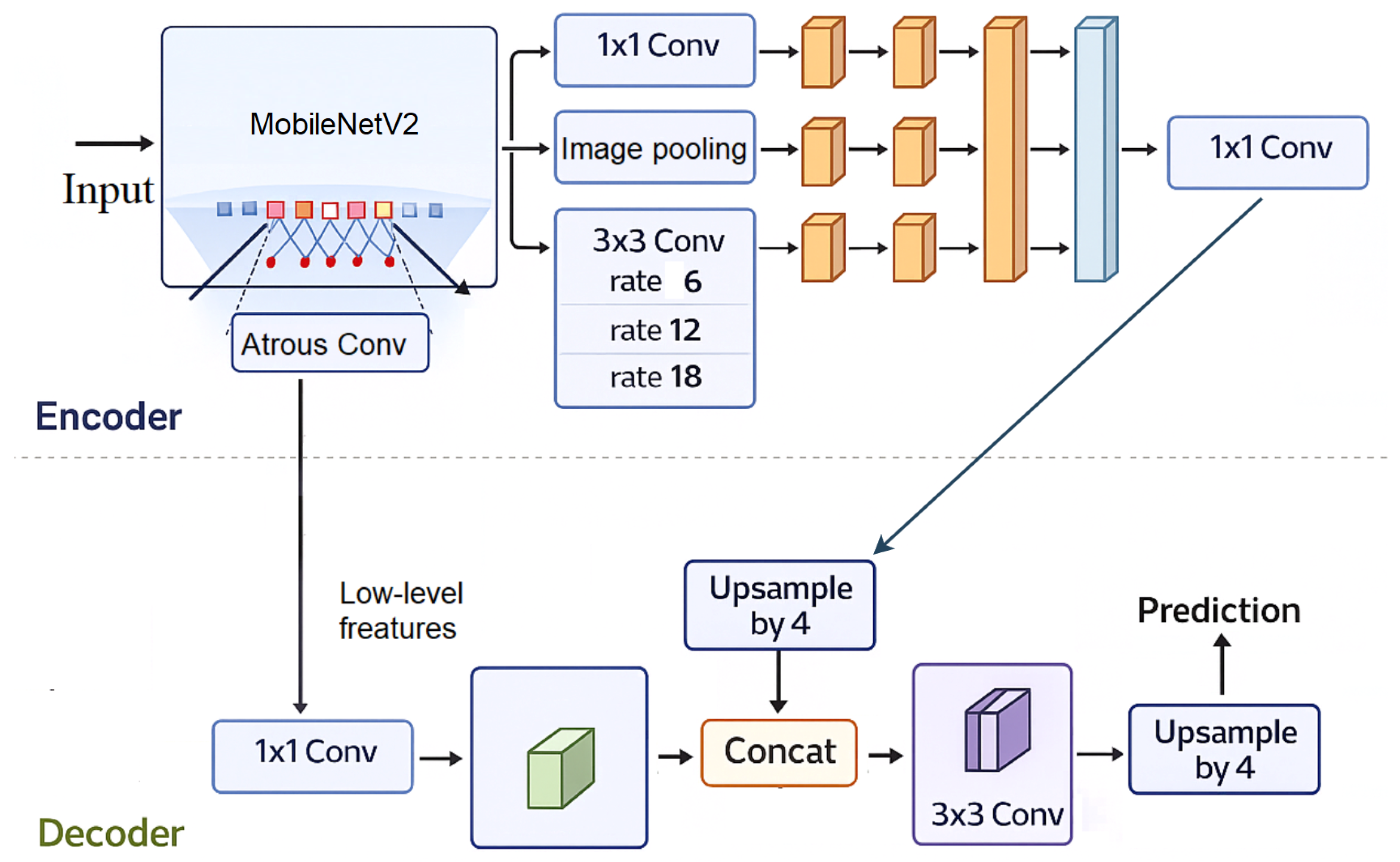
DeepLabV3+ [17] serves as the baseline framework, utilizing an ImageNet-pretrained MobileNetV2 backbone with an output stride of 16. Its core component, the atrous spatial pyramid pooling (ASPP) module, captures multi-scale context via parallel atrous convolutions (rates 6, 12, 18) and global average pooling. The decoder module fuses these high-level semantic features with low-level spatial features (24 channels) from the encoder, refining boundaries through standard convolution layers before bilinear upsampling restores the original resolution. The atrous convolution operation, central to preserving receptive field density, is defined as:
where r is the dilation rate. The full baseline architecture is illustrated in Figure 4.
Figure 4.
DeepLabV3+ baseline architecture with MobileNetV2 encoder, showing atrous convolutions, ASPP module, and decoder with skip connections. Adapted from [17].
3.3. Proposed Model Architecture: Deep-MiSR
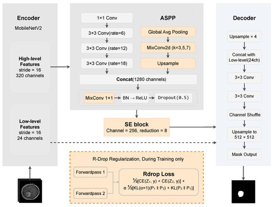
To address the limitations of baseline DeepLabV3+ for heterogeneous tumor segmentation, we introduce Deep-MiSR, which integrates three complementary mechanisms into the encoder–decoder pipeline: mixed depthwise convolutions (MixConv) for multi-scale representation, a squeeze-and-excitation (SE) block for channel recalibration, and R-Drop consistency regularization for training stability. MixConv addresses the fixed receptive field of standard depthwise convolutions, the SE block enhances feature selectivity in tumor-rich regions, and R-Drop mitigates instability arising from severe class imbalance. The full architecture is shown in Figure 5.
Figure 5.
Deep-MiSR architecture. MobileNetV2 encoder at stride 16. MixConv (kernels , , ) replaces depthwise convolutions in ASPP. SE block () recalibrates channels after ASPP. R-Drop regularization applied via dual stochastic passes and symmetric KL divergence.
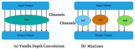
MixConv for multi-scale receptive field diversity. Deep-MiSR replaces selected depthwise convolutions with mixed depthwise convolutions (MixConv) [35]. MixConv assigns heterogeneous kernels to different output-channel groups,
enabling simultaneous extraction of fine-grained boundaries, intermediate textures, and coarse context. MixConv is applied at three sites: (1) the ASPP global-average-pooling branch, (2) the ASPP projection layer, and (3) the decoder refinement blocks (Figure 6).
Figure 6.
MixConv: heterogeneous kernels assigned to different output-channel groups (b) enhance multi-scale feature extraction compare to (a). Adapted from [35].
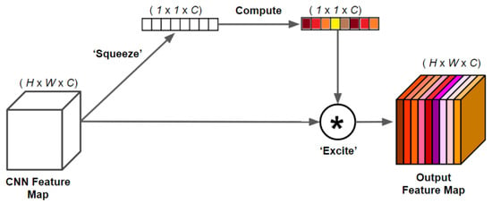
SE block for channel-wise recalibration. A squeeze-and-excitation (SE) block [36] is inserted after ASPP to perform adaptive channel recalibration. Given feature map , global average pooling produces channel descriptors , which pass through a bottleneck with reduction ratio to generate channel weights , where denotes ReLU and denotes sigmoid. The recalibrated output is (Figure 7).
Figure 7.
SE block: global average pooling produces channel descriptors (squeeze), which pass through a bottleneck transformation to generate channel recalibration weights (excitation), adaptively reweighting the input feature map. Adapted from [36].
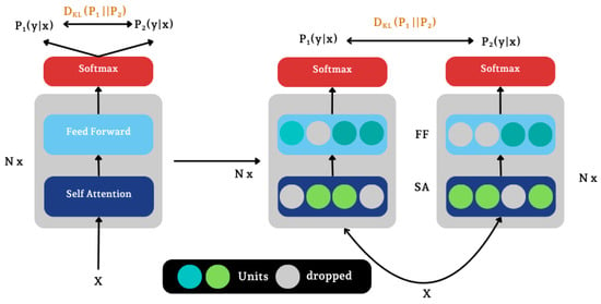
R-Drop consistency regularization. R-Drop [37] enforces output consistency between two stochastic forward passes of the same input. Each training sample is processed twice with independent dropout masks, producing logits and . The total loss combines cross-entropy and symmetric KL divergence:
where . This regularization encourages smoother probability maps and stabilizes training under class imbalance (Figure 8).
Figure 8.
R-Drop regularization: two independent stochastic forward passes of the same input, each with a different dropout mask, produce output distributions and . A symmetric KL divergence loss enforces prediction consistency during training. Adapted from [37].
3.4. Loss Function
Variants without R-Drop (baseline, MixConv, SE Block) are trained with standard pixel-wise cross-entropy. For the R-Drop-containing variants (R-Drop, MixConv + R-Drop, Deep-MiSR), each image is forwarded twice with independent dropout masks, producing logit maps and . The cross-entropy component averages both passes:
where y is the ground-truth label map. A symmetric KL divergence term penalizes disagreement between the two softmax distributions :
This consistency term encourages prediction-stable representations, which is particularly beneficial under the severe class imbalance of this dataset (∼97% background). The total loss is:
with [37]. At inference, a single deterministic forward pass is used; the dual-pass mechanism introduces no additional parameters or overhead at test time.
3.5. Training and Implementation Details
All models were implemented in PyTorch (v1.7.0) and trained on a high-performance server with four NVIDIA RTX 3090 GPUs and dual Intel Xeon Gold 6226R CPUs, running Ubuntu 16.04 with CUDA 11.1 and cuDNN 8.0.4. The MobileNetV2 backbone was initialized with ImageNet pre-trained weights, while decoder layers were initialized using He initialization [46].
Optimization was performed using stochastic gradient descent (SGD) with momentum 0.9 and weight decay . Following DeepLabV3+ [17], a polynomial learning rate schedule (power = 0.9) was applied with an initial learning rate of 0.007. All variants—baseline, ablations (MixConv, SEBlock, R-Drop, MixConv + R-Drop), and the proposed Deep-MiSR—were trained for 300 epochs with a batch size of 4. R-Drop-based models employed the loss in Equation (3) with , while others used standard cross-entropy. Hyperparameters are summarized in Table 1.
Table 1.
Summary of hyperparameters used for model training.
3.6. Evaluation Metrics
Performance was evaluated using five metrics assessing overlap accuracy, precision, and boundary quality. All overlap-based metrics were computed from a global confusion matrix over the entire validation set (), where , , , and denote pixel-level true positives, true negatives, false positives, and false negatives.
Dice Coefficient (Dice). For binary segmentation with classes (background, tumor), per-class Dice is defined as
and the final Dice is the mean over both classes:
Tumor Dice. The foreground-specific Dice (F1-score) is:
Precision (Tumor).
Mean Intersection-over-Union (mIoU).
Hausdorff Distance (HD95). Let and denote predicted and ground-truth tumor contours. The 95th percentile Hausdorff distance is:
Because overlap-based metrics such as Dice are relatively insensitive to localized boundary errors that may arise from acquisition-related artifacts, HD95 is included as a complementary boundary-sensitive measure.
4. Results
This section presents a comprehensive evaluation of Deep-MiSR on the Nanfang T1CE brain tumor segmentation dataset. We first analyze component contributions through ablation and convergence analysis, then compare against prior methods, and finally provide qualitative assessments and practical considerations.
4.1. Ablation Study
To evaluate the individual and combined contributions of MixConv, SE Block, and R-Drop, we incrementally integrated each component into the baseline DeepLabV3+ with MobileNetV2 backbone. All six variants were trained under identical conditions (learning rate = 0.007, 300 epochs, SGD with momentum 0.9). All metrics in Table 2 are computed using the global confusion matrix protocol, wherein true positives, false positives, false negatives, and true negatives are accumulated across all 613 validation images before computing metrics. This pixel-weighted approach differs from per-image averaging (Section 4.4), which weights each image equally regardless of tumor size. Table 2 and Figure 9 summarize the results.
Table 2.
Ablation study on the Nanfang T1CE validation set. Best per metric in bold. ↑: higher is better; ↓: lower is better.
Figure 9.
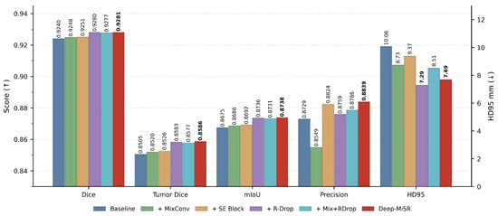
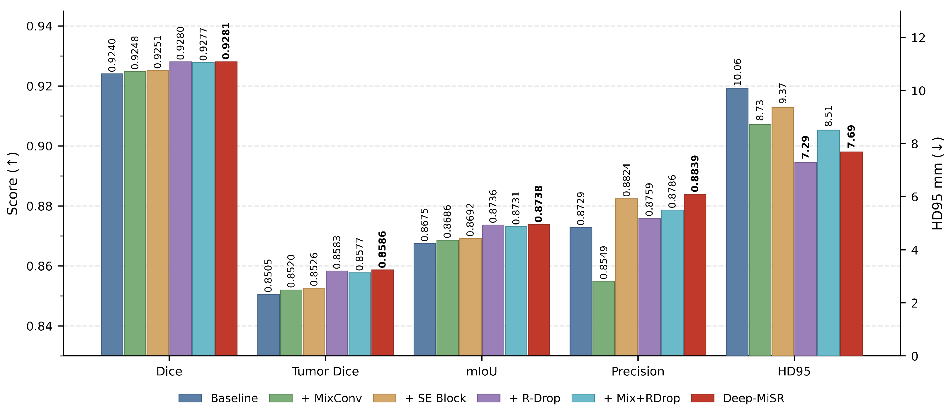
Grouped bar chart of ablation metrics. Overlap-based metrics (Dice, tumor Dice, mIoU, precision; left axis, ↑ higher is better) and boundary distance (HD95; right axis, ↓ lower is better) are shown for all six variants. The proposed Deep-MiSR model (red) achieves the best overlap scores with competitive HD95.
Individual component analysis. R-Drop produced the largest single-component gain, raising Dice by +0.0040 and mIoU by +0.0061 while reducing HD95 by 27.5% (10.06 mm → 7.29 mm), indicating that consistency regularization via symmetric KL divergence is particularly effective near tumor boundaries. SE Block delivered the highest individual precision (0.8824, +0.0095 over baseline) with moderate Dice and mIoU improvements (+0.0011, +0.0017), confirming that channel-wise attention primarily suppresses false positives. MixConv yielded modest overlap gains (Dice +0.0008) and a 13.2% HD95 reduction (10.06 mm → 8.73 mm); however, its precision dropped by 1.8 percentage points, as the multi-kernel design shifted the model toward higher recall at the cost of additional false positives.
Component synergy. The full Deep-MiSR model achieved the best Dice (0.9281), tumor Dice (0.8586), mIoU (0.8738), and precision (0.8839), consistently outperforming all partial configurations (Figure 9). Notably, MixConv + R-Drop alone (Dice = 0.9277) did not surpass R-Drop only (0.9280), yet adding the SE Block in Deep-MiSR restored the gain, indicating that channel recalibration is essential for leveraging multi-scale features under consistency regularization. The marginally higher HD95 of Deep-MiSR (7.69 mm) compared to R-Drop alone (7.29 mm) reflects a minor boundary trade-off, offset by the +0.80 percentage-point precision improvement. These results confirm that R-Drop, MixConv, and SE Block address complementary aspects of segmentation quality, decision boundary stability, spatial multi-scale context, and channel-wise feature selection, and their integration yields additive benefits.
4.2. Convergence Analysis
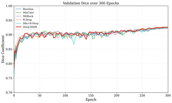
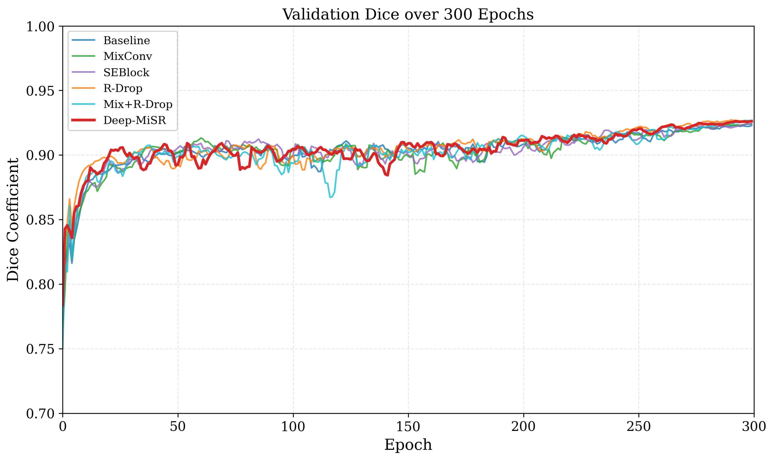
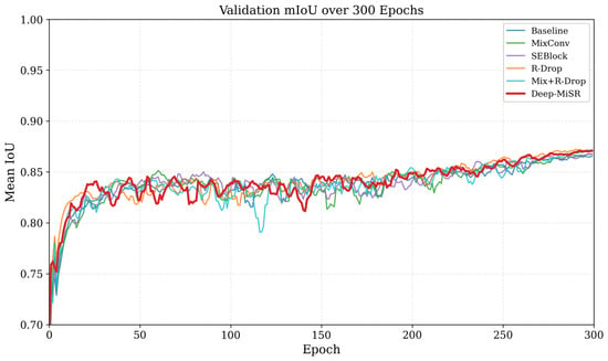
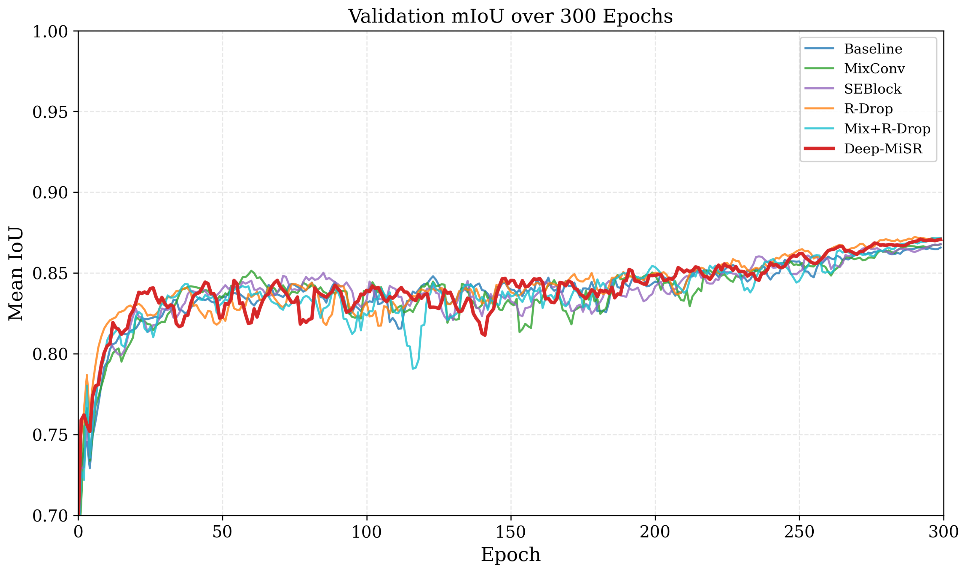
To evaluate training stability across model configurations, validation Dice and mIoU scores were monitored over the complete 300-epoch training schedule. The convergence behavior of all six architectural variants is illustrated in Figure 10 and Figure 11.
Figure 10.
Validation Dice over 300 training epochs for all six ablation variants. The Dice score demonstrates stable and monotonic improvement during training without signs of divergence.
Figure 11.
Validation mIoU over 300 training epochs. The best validation mIoU is typically achieved between epochs 284 and 293, while performance gradually increases after approximately epoch 200.
All model variants exhibit smooth and consistent convergence behavior throughout training, with no evidence of optimization collapse. The proposed architectural components, including MixConv, SE Block, and R-Drop regularization, do not introduce instability during learning, as the enhanced models maintain convergence patterns comparable to the baseline while achieving higher performance ceilings. The alignment between training progression and validation performance further indicates strong generalization capability across all configurations under the 300-epoch training schedule.
4.3. Comparison with Prior Methods on Nanfang Dataset
To contextualize the performance of Deep-MiSR, we compared our results with four methods previously evaluated on the Nanfang T1CE dataset. Table 3 summarizes the available metrics. All methods were trained and tested on the same single-modality T1-weighted contrast-enhanced MRI data, enabling direct comparison.
Table 3.
Comparison with existing methods on the Nanfang T1CE dataset. Best values in bold. Dash (–) indicates metric not reported in the original publication.
Deep-MiSR achieved the highest Dice (0.9281) and mIoU (0.8738) among all compared methods. Relative to the nearest competitor YOLO-BT, our method improved Dice by +0.0021 and mIoU by +0.0108 (+1.25%). The margin over earlier methods is more pronounced: +0.0786 Dice over R2UNet and +0.1994 over the 2021 convolutional autoencoder, reflecting steady progress on this benchmark. Although the absolute improvement over recent methods is modest, the result demonstrates that targeted enhancements to an established encoder–decoder architecture can match or exceed more complex detection-oriented frameworks such as YOLO-BT.
A notable gap in Table 3 is that no prior study on this dataset reported boundary-based metrics. Our HD95 of 7.69 mm therefore establishes the first boundary precision benchmark for Nanfang T1CE segmentation. For reference, recent multimodal approaches on BraTS (utilizing four MRI sequences) typically report median HD95 values above 8 mm [47], suggesting that our single-modality result is competitive despite using substantially less input information.
4.4. Statistical Validation
We assessed the statistical significance of performance differences using two complementary procedures: (i) a per-image paired Wilcoxon signed-rank test and (ii) a non-parametric bootstrap confidence interval on global metrics.
Per-image paired testing. Per-image Dice and mIoU were computed for all six variants across validation images. Because per-image metrics exhibit strong skew from trivially easy and challenging cases, violating the normality assumption, we employed the Wilcoxon signed-rank test [48], a non-parametric paired test on the ranks of within-image differences, to evaluate whether the median paired difference equals zero. Note that per-image and global metrics differ in absolute value (e.g., baseline per-image Dice vs. global Dice ) because the former weights images equally while the latter weights pixels equally; the global values in Table 2 remain the primary evaluation.
As shown in Table 4, all R-Drop-containing variants achieve for both metrics, identifying R-Drop as the principal contributor. MixConv alone is significant but modest ( for Dice), while SE Block alone does not reach (), suggesting its benefit emerges through synergy with the other components. Effect sizes are small (Cohen’s for Dice; for mIoU), consistent with the high baseline performance (Dice ).
Table 4.
Per-image Wilcoxon signed-rank test versus baseline (). †: ; *: .
Bootstrap confidence intervals. We constructed 95% bootstrap CIs by resampling images with replacement over iterations, accumulating a global confusion matrix per resample, and recording the Dice and mIoU difference between Deep-MiSR and baseline. Both CIs exclude zero (Dice: ; mIoU: ), with Deep-MiSR outperforming the baseline in 98.5% of resamples.
In summary, both the per-image Wilcoxon test () and bootstrap CIs confirm that the improvement of Deep-MiSR over the baseline is statistically significant and robust to sampling variability.
4.5. Visual Comparison of Segmentation Results
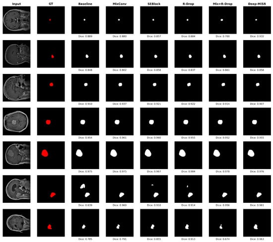
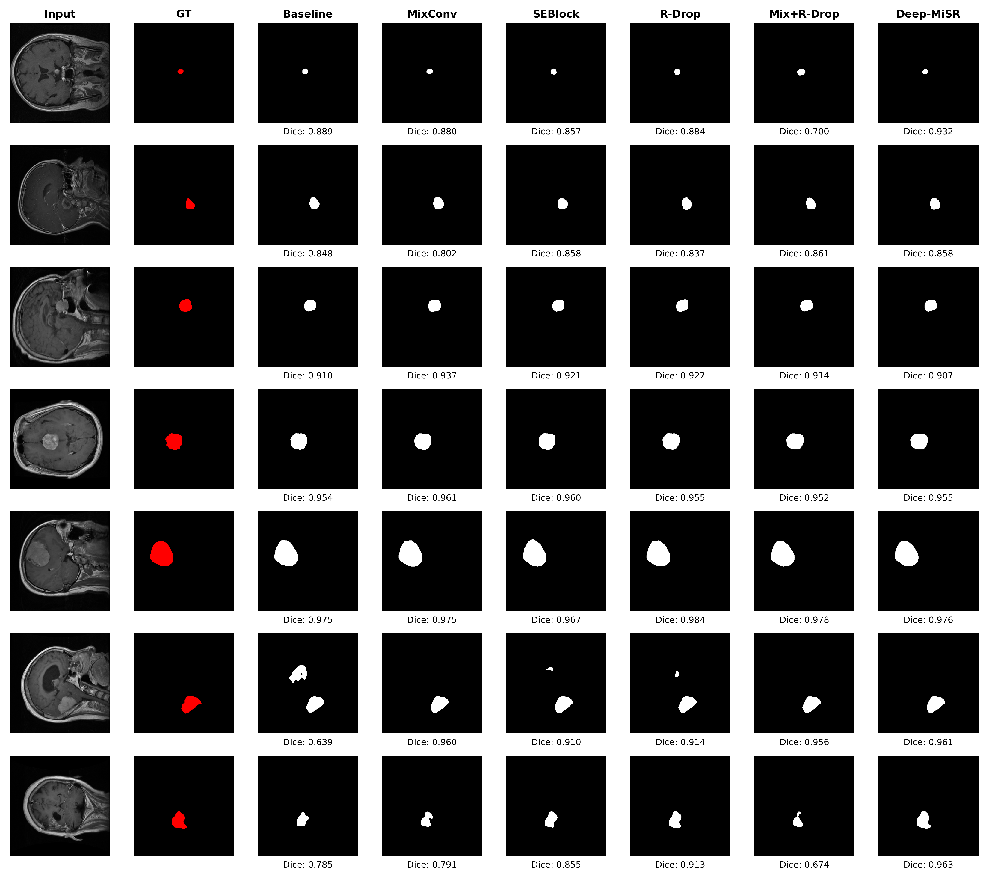
To complement the quantitative analysis, Figure 12 presents segmentation outputs from all six model configurations across seven representative test slices, with per-slice DSC annotated below each prediction.
Figure 12.
Segmentation comparison across six configurations on seven axial brain MRI slices. Columns: input image, ground truth (red), baseline, MixConv, SEBlock, R-Drop, MixConv + R-Drop, and Deep-MiSR predictions (white), with per-slice DSC values annotated. Deep-MiSR achieves consistently higher boundary fidelity, particularly for small or morphologically complex lesions (slices 6 and 7).
All models produce coherent masks for larger, well-circumscribed lesions (slices 3–5, DSC broadly exceeding 0.90), indicating that such cases are within the representational capacity of the baseline architecture. Differences emerge on slices with small, irregular, or low-contrast tumors. In slice 6, the baseline yields a fragmented prediction (), whereas Deep-MiSR produces a spatially coherent mask (). Slice 7 similarly exposes limitations of the baseline () and MixConv + R-Drop (), while Deep-MiSR maintains strong boundary fidelity ().
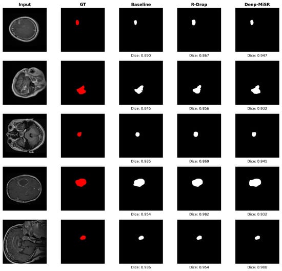
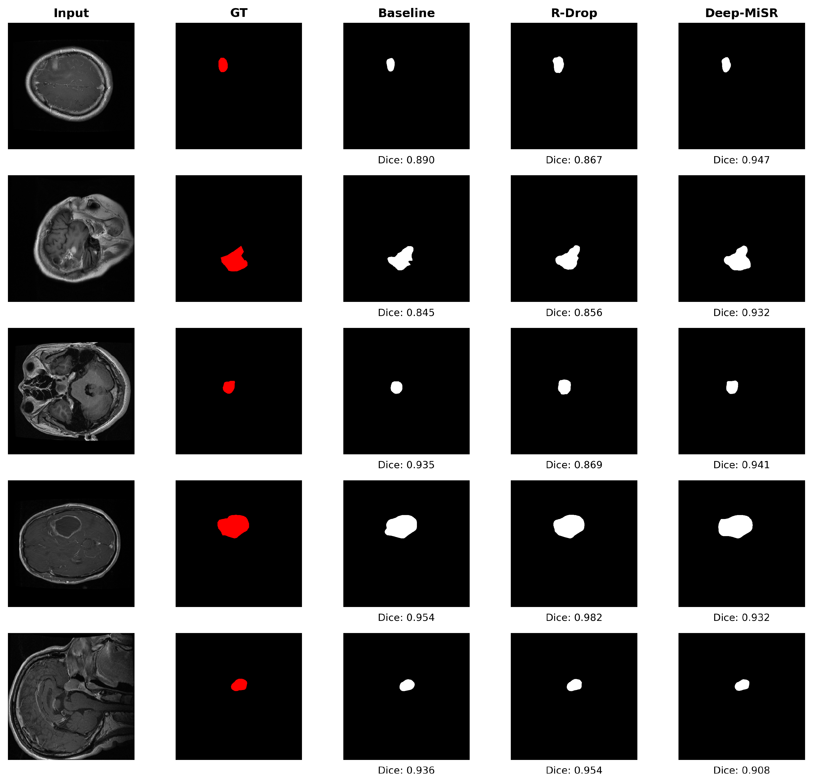
Figure 13 provides a focused comparison of baseline, R-Drop, and Deep-MiSR on five additional slices, isolating the individual and combined contributions of the regularization strategy and the full framework. Deep-MiSR achieves the highest DSC on slices 1–3 (, , ), outperforming both baseline (, , ) and R-Drop (, , ) on small and irregularly shaped lesions. R-Drop alone does not consistently improve over the baseline on these cases, suggesting that stochastic regularization in isolation is insufficient for low-contrast or small-target segmentation. On slices 4–5, which feature larger and more homogeneous tumors, all three models yield comparable DSC values, confirming that the gains from Deep-MiSR are most consequential in challenging scenarios.
Figure 13.
Focused three-model comparison on five axial slices. Columns: input image, ground truth (red), baseline, R-Drop, and Deep-MiSR predictions (white), with per-slice DSC annotated. Deep-MiSR yields the highest DSC on slices with small and irregular lesions (slices 1–3), while all models perform comparably on larger tumors (slices 4–5).
4.6. Failure Case Analysis
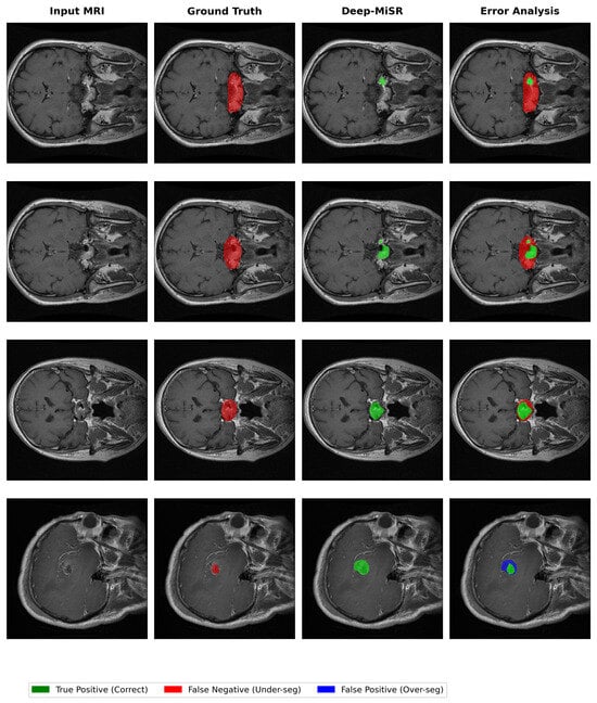
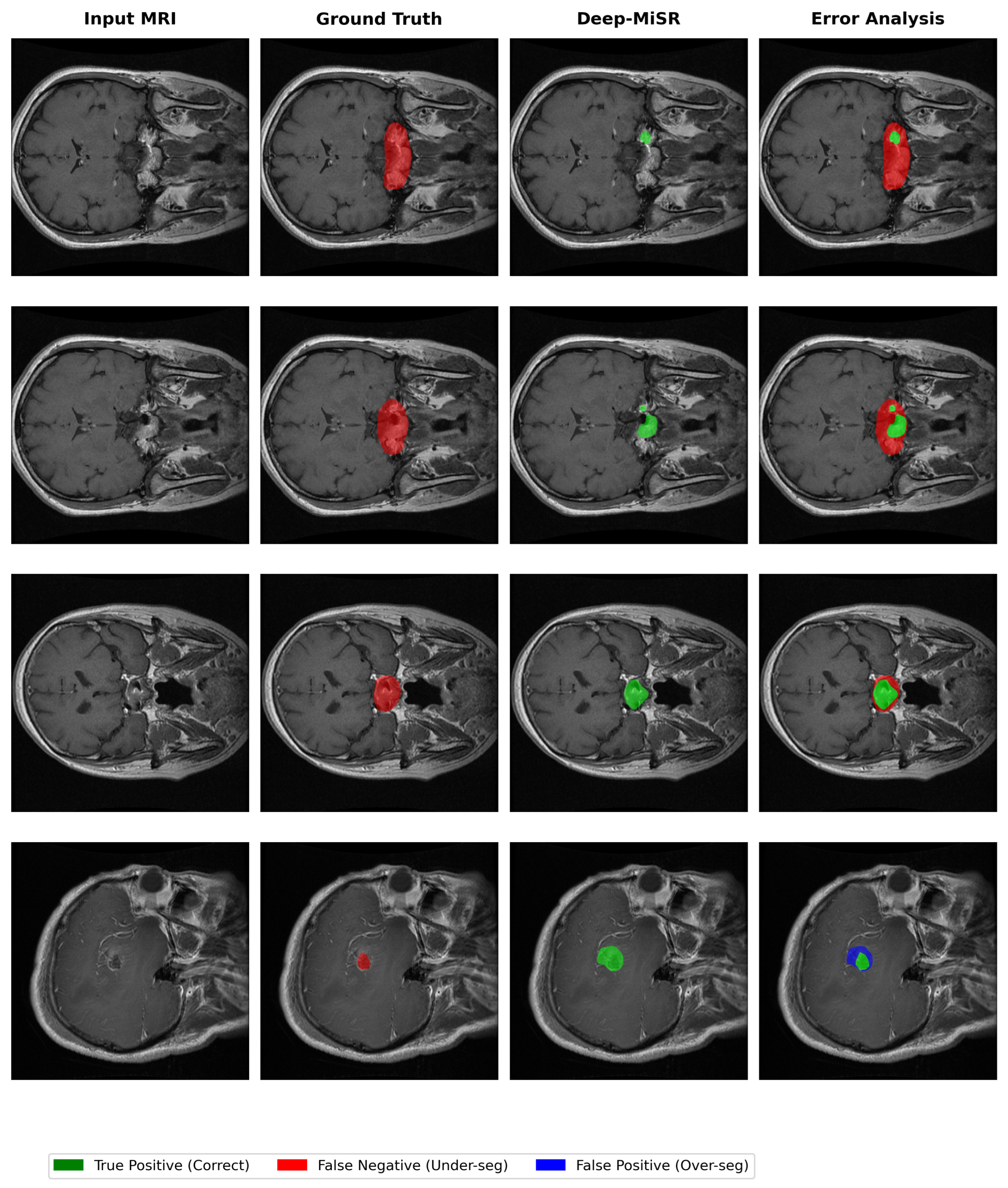
To characterize Deep-MiSR’s behavior under challenging conditions, we examined cases with suboptimal predictions on the validation set. Figure 14 presents representative examples illustrating two distinct patterns.
Figure 14.
Representative challenging cases for Deep-MiSR. Columns: input MRI, ground truth, Deep-MiSR prediction, and error map (green = true positive, red = false negative, blue = false positive). The first three rows illustrate varying degrees of under-segmentation, while the fourth row demonstrates over-segmentation of a small tumor.
The predominant pattern is conservative under-segmentation, where predictions remain within the ground truth boundary (). As shown in the first three rows of Figure 14, this ranges from minimal coverage (Dice = 0.13, ∼7%) through moderate detection (Dice = 0.40, ∼25%) to near-complete delineation with residual boundary imprecision (Dice = 0.76, ∼62%). The consistent absence of false positives indicates that the model preserves high precision even in difficult cases, a clinically preferable behavior that avoids misidentifying healthy tissue as tumor.
A less frequent pattern is over-segmentation, shown in the bottom row of Figure 14, where the model achieves complete tumor recall () but extends beyond the true boundary (∼191% over-extension, Dice = 0.51). This pattern is primarily associated with small tumors exhibiting ambiguous tissue contrast.
These complementary patterns, high-precision under-segmentation and high-recall over-segmentation, represent consistent directional characteristics rather than random errors. This aligns with the tumor size stratification analysis, where mean Dice ranges from 0.779 for small tumors to 0.854 for large tumors, confirming tumor size as the primary factor influencing segmentation difficulty. Boundary-aware loss functions and uncertainty-guided refinement represent promising directions to improve sensitivity for small tumors while preserving the low false-positive rate.
4.7. Model Complexity and Practical Considerations
Beyond segmentation accuracy, the computational cost of each architectural component is an important consideration for practical deployment. To quantify this, we measured the parameter count, floating-point operations (FLOPs), inference latency, and peak GPU memory for all six ablation variants. FLOPs were computed analytically for a single 513 × 513 input. Latency and memory were measured on an NVIDIA GeForce RTX 2060 GPU (6 GB VRAM) with batch size of 1, reporting the mean and standard deviation over 20 runs following 5 warmup iterations. Note that all models were trained on the high-performance server described in Section 3; the RTX 2060 was used exclusively for inference benchmarking to reflect performance on consumer-grade hardware. The results are summarized in Table 5.
Table 5.
Model complexity comparison across ablation variants. FLOPs are computed for a single 513 × 513 input. Latency and memory measured on an NVIDIA GeForce RTX 2060 GPU (mean ± std over 20 runs).
As shown in Table 5, the computational overhead in Deep-MiSR originates almost entirely from the MixConv module, which replaces standard 3 × 3 convolutions with three parallel depthwise branches (3 × 3, 5 × 5, 7 × 7 kernels) in both the ASPP and decoder stages, increasing parameters from 5.81 M to 13.77 M (+137%) and FLOPs from 53.97 G to 106.60 G (+97%). The SE Block adds only 16,384 parameters (+0.3%), corresponding to two fully connected layers (), with no measurable impact on FLOPs or latency. R-Drop introduces no additional inference-time parameters, as its symmetric KL-divergence consistency loss operates exclusively during training; at test time, only a single deterministic forward pass is required. Channel shuffle is a parameter-free tensor reshape operation that contributes negligible computational overhead.
Despite the increase in model size relative to the baseline, the complete Deep-MiSR model processes a single 513 × 513 slice in 42.7 ms on the RTX 2060, corresponding to a throughput of approximately 23 slices per second. For a study comprising 613 slices, total inference time is approximately 26 s, with peak GPU memory remaining under 524 MB. These results indicate that the segmentation improvements reported in Section 4.1 (Dice +0.0041, HD95 −2.37 mm over baseline) are achieved at a computational cost that remains feasible on widely available consumer-grade GPU hardware.
5. Discussion
This study investigated whether targeted architectural enhancements to DeepLabV3+, namely heterogeneous-kernel MixConv, squeeze-and-excitation (SE) channel recalibration, and R-Drop consistency regularization, can yield meaningful improvements in brain tumor segmentation on single-modality T1CE MRI. On the Nanfang T1CE dataset, under a fixed 80/20 slice-wise split ( validation images), the proposed Deep-MiSR model achieved a Dice coefficient of 0.9281, mIoU of 0.8738, precision of 0.8839, and HD95 of 7.69 mm (Table 2), outperforming all ablation variants and previously published methods evaluated under identical conditions (Table 3). These gains were confirmed as statistically significant by both a paired Wilcoxon signed-rank test () and bootstrap confidence intervals excluding zero (Section 4.4). The following subsections interpret the experimental findings, discuss clinical implications, and identify the principal limitations of the current work.
5.1. Component Contributions and Architectural Synergy
The ablation results (Table 2) reveal that each architectural component addresses a distinct aspect of segmentation quality, and that these contributions are complementary. R-Drop consistency regularization produced the largest individual gains, raising Dice by +0.0040 and mIoU by +0.0061 over the baseline while reducing HD95 by 27.5% (from 10.06 mm to 7.29 mm). By enforcing agreement between dual stochastic forward passes via symmetric KL divergence, R-Drop regularizes the decision boundary under severe class imbalance (∼97% background), where standard cross-entropy tends to underfit the minority tumor class. The statistical analysis (Table 4) corroborates this finding: all R-Drop-containing variants achieved on the paired Wilcoxon test, identifying R-Drop as the principal contributor to per-image improvement.
MixConv contributed more modestly to overlap measures (+0.0008 Dice) but achieved a 13.2% HD95 reduction (10.06 mm → 8.73 mm) through multi-scale spatial encoding with heterogeneous kernels (, , ), indicating that boundary delineation benefits from richer receptive-field diversity. However, MixConv reduced precision by 1.8 percentage points (from 0.8729 to 0.8549), reflecting a shift toward higher recall at the cost of additional false positives. The SE Block counterbalanced this effect, providing the highest single-component precision (0.8824, +0.0095 over baseline) through adaptive channel recalibration with negligible computational overhead (Table 5: +16,384 parameters, +0.3%). Notably, the SE Block alone did not reach significance at on the Wilcoxon test (), suggesting that its benefit emerges primarily through synergy with the other components rather than as an independent gain.
The synergistic nature of the three components is most evident when comparing the full model (Dice = 0.9281, precision = 0.8839) against the MixConv + R-Drop variant (Dice = 0.9277, precision = 0.8786). Despite integrating two individually beneficial mechanisms, MixConv + R-Drop did not surpass R-Drop alone (Dice = 0.9280), confirming that SE Block channel recalibration is essential for resolving the precision–recall tension introduced by multi-kernel convolutions. Deep-MiSR achieves the highest precision among all variants while simultaneously attaining the best Dice and mIoU, demonstrating that R-Drop stabilizes predictions, MixConv enriches spatial context, and the SE Block refines feature selectivity—jointly optimizing complementary aspects of segmentation quality.
5.2. Comparison with Existing Methods
Comparison with prior results on the Nanfang T1CE dataset (Table 3) further supports the proposed approach. Deep-MiSR achieved the highest Dice (0.9281) and mIoU (0.8738) among all compared methods, surpassing YOLO-BT (Dice = 0.9260) [29] by +0.0021, EfficientNet-UNet (Dice = 0.9130) [30] by +0.0151, and R2UNet (Dice = 0.8495) [31] by +0.0786. The improvement over the 2021–2025 period—from 0.7287 (convolutional autoencoder [32]) to 0.9281 (Deep-MiSR), illustrates steady progress on this benchmark. Although the absolute margin over YOLO-BT is modest, the result demonstrates that targeted enhancements to an established encoder–decoder architecture can match or exceed more complex detection-oriented frameworks while providing systematic multi-metric evaluation (overlap and boundary precision) not reported in prior work.
A notable contribution is the introduction of boundary-based evaluation for this dataset. No prior study on Nanfang T1CE reported HD95 or related boundary metrics; the value of 7.69 mm therefore establishes the first boundary precision benchmark. For reference, recent multimodal approaches on BraTS utilizing four MRI sequences typically report median HD95 values above 8 mm [47], suggesting that Deep-MiSR’s single-modality boundary performance is competitive despite using substantially less input information.
5.3. Clinical Considerations
The multi-metric evaluation framework adopted in this study underscores that boundary metrics exhibit greater sensitivity to architectural variations than overlap measures alone. While the Dice difference between the baseline and Deep-MiSR is 0.0041, the corresponding HD95 improvement is 2.37 mm (23.6%), consistent with prior observations that boundary-based metrics more faithfully capture delineation quality in imbalanced segmentation tasks [49,50]. Improved boundary localization is directly relevant for pre-contouring workflows in radiotherapy planning, where accurate initial contours reduce the manual annotation burden while preserving radiologist oversight.
From a deployment perspective, the complexity analysis (Table 5) shows that Deep-MiSR processes a single 513 × 513 slice in 42.7 ms on a mid-range GPU (RTX 2060), yielding approximately 26 s of total inference for a complete 613-slice study, with peak memory under 524 MB. These characteristics are compatible with clinical screening workflows on consumer-grade hardware. The convergence analysis (Section 4.2) further confirms that the architectural modifications do not introduce training instability; all six variants converge smoothly over the 300-epoch schedule, with the best validation performance reached between epochs 284 and 293.
The qualitative failure analysis (Section 4.6) revealed that conservative under-segmentation with zero false positives is the predominant failure mode, a clinically preferable behavior that avoids misidentifying healthy tissue as tumor. Over-segmentation was observed primarily for small tumors with ambiguous tissue contrast. This aligns with the tumor size stratification analysis, where mean Dice ranges from 0.779 for small tumors to 0.854 for large tumors, identifying tumor size as the principal determinant of segmentation difficulty.
However, important limitations for clinical application should be acknowledged. The current design operates on T1CE alone, which primarily captures the enhancing tumor core. For infiltrative gliomas, additional sequences (T2, FLAIR) provide complementary information about edema and non-enhancing tumor components not visualized on T1CE [7]. The model is therefore most suited as computer-aided detection assistance for well-circumscribed tumors (meningiomas, pituitary adenomas), with mandatory radiologist review.
5.4. Limitations and Future Directions
Several limitations of this study warrant discussion. First, all experiments were conducted on a single institutional dataset with a fixed 80/20 slice-wise train–validation split. Slice-wise random partitioning may introduce inter-slice correlation between training and validation sets, potentially inflating reported performance relative to patient-wise splitting. Although the statistical validation (Section 4.4) confirmed that improvements are significant using both paired testing () and bootstrap confidence intervals (Dice CI: ; mIoU CI: ; Deep-MiSR superior in 98.5% of resamples), these analyses operate within the existing split. Multi-institutional validation with strict patient-wise partitioning is necessary to rigorously assess generalization. Furthermore, as the Nanfang dataset is a single-institution archive, patient-level metadata including clinical histories, scanner specifications, and scan duration are not publicly reported, precluding formal assessment of cohort homogeneity or acquisition-related noise variability. In addition, robustness to variations in image contrast, brightness, and scanner-specific intensity scaling, as encountered when applying the model to images from alternative acquisition protocols or institutions, has not been evaluated and remains an open question for future cross-dataset validation studies.
Second, the 2D slice-by-slice processing inherent to the current architecture ignores inter-slice spatial relationships. Volumetric extensions (3D or 2.5D) that leverage axial continuity could improve segmentation consistency across consecutive slices, particularly for tumors with heterogeneous enhancement patterns.
Third, the tumor size stratification analysis revealed that mean Dice ranges from 0.779 for small tumors to 0.854 for large tumors, indicating substantial size-dependent performance variation. Boundary-aware loss functions and hard-example mining strategies may help close this gap. It is also plausible that acquisition-related noise contributes to contrast ambiguity in small lesions and thereby influences the over-segmentation behavior observed in Section 4.6; disentangling these effects would require per-slice image quality metrics not currently available in the public dataset.
Finally, uncertainty quantification is absent from the current framework. Ensemble methods or Monte Carlo dropout could enable the identification of low-confidence predictions, providing radiologists with actionable reliability signals during clinical review. Beyond technical validation, demonstrating the clinical impact of Deep-MiSR will ultimately require prospective randomized trials evaluating its effect on clinically meaningful endpoints, such as radiotherapy planning efficiency, surgical outcomes, or longitudinal response assessment accuracy.
6. Conclusions
This work presented Deep-MiSR, an enhanced DeepLabV3+ framework for single-modality brain tumor segmentation on contrast-enhanced T1-weighted MRI. By integrating heterogeneous-kernel MixConv, SE-based channel recalibration, and R-Drop consistency regularization, the proposed model addresses key challenges of medical image segmentation under severe class imbalance through complementary architectural and training-time enhancements.
On the Nanfang T1CE validation set (), Deep-MiSR achieved a Dice of 0.9281, mIoU of 0.8738, precision of 0.8839, and HD95 of 7.69 mm, surpassing all previously published results on this dataset, including R2UNet [31], EfficientNet-UNet [30], and YOLO-BT [29] (Table 3). Systematic ablation demonstrated that each component contributes measurably: R-Drop provides the largest individual gain (Dice +0.0040, HD95 −27.5%), MixConv enhances boundary fidelity (HD95 −13.2%), and the SE Block recovers precision (+0.0095) lost to multi-kernel feature expansion. These improvements were confirmed as statistically significant via paired Wilcoxon testing () and bootstrap confidence intervals that exclude zero, with Deep-MiSR outperforming the baseline in 98.5% of 10,000 bootstrap resamples.
This study further establishes the first boundary precision benchmark (HD95) for the Nanfang T1CE dataset and demonstrates that comprehensive multi-metric evaluation, encompassing overlap, boundary, and precision–recall measures together with formal statistical validation, is essential for assessing clinical deployment readiness. Future work will prioritize patient-wise multi-institutional validation, volumetric extensions incorporating inter-slice context, and uncertainty quantification to support clinical decision-making workflows. The architectural framework demonstrated here combines multi-scale representation, channel selectivity, and consistency regularization, which represents a generalizable approach applicable to other medical imaging segmentation tasks characterized by severe class imbalance.
Author Contributions
Conceptualization, M.P.M. and J.Z.; methodology, M.P.M.; software, M.P.M.; validation, M.P.M., J.S. and J.Z.; formal analysis, M.P.M.; writing—original draft preparation, M.P.M.; writing—review and editing, J.S. and J.Z.; visualization, M.P.M.; supervision, J.Z.; project administration, J.Z.; funding acquisition, J.Z. All authors have read and agreed to the published version of the manuscript.
Funding
This research was funded by the National Natural Science Foundation of China, grant number 52171310.
Institutional Review Board Statement
Not applicable.
Informed Consent Statement
Not applicable.
Data Availability Statement
The data presented in this study are openly available on Figshare https://figshare.com/articles/dataset/brain_tumor_dataset/1512427/5 (accessed on 10 April 2026).
Acknowledgments
The authors would like to thank the project supervisor, Jing Zhang, for guidance and support throughout the development of this work.
Conflicts of Interest
The authors declare no conflicts of interest.
Abbreviations
The following abbreviations are used in this manuscript:
| ASPP | Atrous Spatial Pyramid Pooling |
| CE | Cross-Entropy |
| CNN | Convolutional Neural Network |
| Dice | Dice Similarity Coefficient |
| HD95 | 95th Percentile Hausdorff Distance |
| IoU | Intersection over Union |
| KL | Kullback–Leibler Divergence |
| mIoU | Mean Intersection over Union |
| MRI | Magnetic Resonance Imaging |
| R-Drop | Regularized Dropout (symmetric KL-based consistency regularization) |
| SE | Squeeze-and-Excitation |
| T1CE | Contrast-Enhanced T1-Weighted MRI |
| MiSR | MixConv–SE–R-Drop |
References
- Kim, S.; Son, Y.; Oh, J.; Kim, S.; Jang, W.; Lee, S.; Smith, L.; Pizzol, D.; Lee, J.; Lee, H.; et al. Global burden of brain and central nervous system cancer in 185 countries, and projections up to 2050: A population-based systematic analysis of GLOBOCAN 2022. J. Neuro-Oncol. 2025, 175, 673–685. [Google Scholar] [CrossRef] [Scilit] [PubMed]
- Stupp, R.; Mason, W.P.; van den Bent, M.J.; Weller, M.; Fisher, B.; Taphoorn, M.J.B.; Belanger, K.; Brandes, A.A.; Marosi, C.; Bogdahn, U.; et al. Radiotherapy plus Concomitant and Adjuvant Temozolomide for Glioblastoma. N. Engl. J. Med. 2005, 352, 987–996. [Google Scholar] [CrossRef] [Scilit] [PubMed]
- Ostrom, Q.T.; Price, M.; Neff, C.; Cioffi, G.; Waite, K.A.; Kruchko, C.; Barnholtz-Sloan, J.S. CBTRUS Statistical Report: Primary Brain and Other Central Nervous System Tumors Diagnosed in the United States in 2016–2020. Neuro-Oncology 2023, 25, ii1–ii99. [Google Scholar] [CrossRef] [Scilit]
- Brown, T.J.; Brennan, M.C.; Li, M.; Church, E.W.; Brandmeir, N.J.; Rakszawski, K.L.; Patel, A.S.; Rizk, E.B.; Suki, D.; Sawaya, R.; et al. Association of the Extent of Resection with Survival in Glioblastoma. JAMA Oncol. 2016, 2, 1460–1469. [Google Scholar] [CrossRef] [Scilit]
- Zhu, Z.; Wang, Z.; Qi, G.; Mazur, N.; Yang, P.; Liu, Y. Brain Tumor Segmentation in MRI with Multi-Modality Spatial Information Enhancement and Boundary Shape Correction. Pattern Recognit. 2024, 153, 110553. [Google Scholar] [CrossRef] [Scilit]
- Martucci, M.; Russo, R.; Schimperna, F.; D’Apolito, G.; Panfili, M.; Grimaldi, A.; Perna, A.; Ferranti, A.M.; Varcasia, G.; Giordano, C.; et al. Magnetic Resonance Imaging of Primary Adult Brain Tumors: State of the Art and Future Perspectives. Biomedicines 2023, 11, 364. [Google Scholar] [CrossRef] [Scilit]
- Menze, B.H.; Jakab, A.; Bauer, S.; Kalpathy-Cramer, J.; Farahani, K.; Kirby, J.; Burren, Y.; Porz, N.; Slotboom, J.; Wiest, R.; et al. The Multimodal Brain Tumor Image Segmentation Benchmark (BRATS). IEEE Trans. Med. Imaging 2014, 34, 1993–2024. [Google Scholar] [CrossRef] [Scilit]
- Iratni, M.; Abdullah, A.; Aldhaheri, M.; Elharrouss, O.; Abd-alrazaq, A.; Rustamov, Z.; Zaki, N.; Damseh, R. Transformers for Neuroimage Segmentation: Scoping Review. J. Med. Internet Res. 2025, 27, e57723. [Google Scholar] [CrossRef] [Scilit]
- Wen, P.Y.; Macdonald, D.R.; Reardon, D.A.; Cloughesy, T.F.; Sorensen, A.G.; Galanis, E.; DeGroot, J.; Wick, W.; Gilbert, M.R.; Lassman, A.B.; et al. Updated response assessment criteria for high-grade gliomas: Response assessment in neuro-oncology working group. J. Clin. Oncol. 2010, 28, 1963–1972. [Google Scholar] [CrossRef] [Scilit]
- Litjens, G.; Kooi, T.; Bejnordi, B.E.; Setio, A.A.A.; Ciompi, F.; Ghafoorian, M.; van der Laak, J.A.W.M.; van Ginneken, B.; Sánchez, C.I. A Survey on Deep Learning in Medical Image Analysis. Med. Image Anal. 2017, 42, 60–88. [Google Scholar] [CrossRef] [Scilit]
- Ronneberger, O.; Fischer, P.; Brox, T. U-Net: Convolutional Networks for Biomedical Image Segmentation. In Lecture Notes in Computer Science, Proceedings of the Medical Image Computing and Computer-Assisted Intervention—MICCAI 2015; Springer: Berlin/Heidelberg, Germany, 2015; Volume 9351, pp. 234–241. [Google Scholar] [CrossRef] [Scilit]
- Isensee, F.; Jaeger, P.F.; Kohl, S.A.A.; Petersen, J.; Maier-Hein, K.H. nnU-Net: A self-configuring method for deep learning-based biomedical image segmentation. Nat. Methods 2021, 18, 203–211. [Google Scholar] [CrossRef] [Scilit] [PubMed]
- Hatamizadeh, A.; Tang, Y.; Nath, V.; Yang, D.; Myronenko, A.; Landman, B.; Roth, H.; Xu, D. UNETR: Transformers for 3D Medical Image Segmentation. In Proceedings of the IEEE Winter Conference on Applications of Computer Vision (WACV), Waikoloa, HI, USA, 3–8 January 2022. [Google Scholar] [CrossRef] [Scilit]
- Tang, Y.; Yang, D.; Li, W.; Roth, H.; Landman, B.; Xu, D.; Nath, V.; Hatamizadeh, A. Self-Supervised Pre-Training of Swin Transformers for 3D Medical Image Analysis. In Proceedings of the Proceedings of the IEEE/CVF Conference on Computer Vision and Pattern Recognition (CVPR), New Orleans, LA, USA, 18–24 June 2022. [Google Scholar] [CrossRef] [Scilit]
- Bonato, B.; Nanni, L.; Bertoldo, A. Advancing Precision: A Comprehensive Review of MRI Segmentation Datasets from BraTS Challenges (2012–2025). Sensors 2025, 25, 1838. [Google Scholar] [CrossRef] [Scilit] [PubMed]
- Ngo, D.K.; Tran, M.T.; Kim, S.H.; Yang, H.J.; Lee, G.S. Multi-Task Learning for Small Brain Tumor Segmentation from MRI. Appl. Sci. 2020, 10, 7790. [Google Scholar] [CrossRef] [Scilit]
- Chen, L.C.; Zhu, Y.; Papandreou, G.; Schroff, F.; Adam, H. Encoder-Decoder with Atrous Separable Convolution for Semantic Image Segmentation. In Proceedings of the European Conference on Computer Vision (ECCV); Springer Science & Business Media: Berlin/Heidelberg, Germany, 2018; pp. 833–851. [Google Scholar] [CrossRef] [Scilit]
- Wang, J.; Liu, X. Medical image recognition and segmentation of pathological slices of gastric cancer based on Deeplab v3+ neural network. Comput. Methods Programs Biomed. 2021, 207, 106210. [Google Scholar] [CrossRef] [Scilit]
- Ketenci Çay, F.; Yeşil, Ç.; Çay, O.; Yılmaz, B.G.; Özçini, F.H.; İlgüy, D. DeepLabv3 + method for detecting and segmenting apical lesions on panoramic radiography. Clin. Oral Investig. 2025, 29, 101. [Google Scholar] [CrossRef] [Scilit]
- Zhou, Z.; Siddiquee, M.M.R.; Tajbakhsh, N.; Liang, J. UNet++: A Nested U-Net Architecture for Medical Image Segmentation. In Deep Learning in Medical Image Analysis and Multimodal Learning for Clinical Decision Support; Lecture Notes in Computer Science; Springer: Berlin/Heidelberg, Germany, 2018; Volume 11045, pp. 3–11. [Google Scholar] [CrossRef] [Scilit]
- Badrinarayanan, V.; Kendall, A.; Cipolla, R. SegNet: A Deep Convolutional Encoder-Decoder Architecture for Image Segmentation. IEEE Trans. Pattern Anal. Mach. Intell. 2017, 39, 2481–2495. [Google Scholar] [CrossRef] [Scilit]
- Pourmahboubi, A.; Saeed, N.A.; Tabrizchi, H. A brain tumor segmentation enhancement in MRI images using U-Net and transfer learning. BMC Med. Imaging 2025, 25, 307. [Google Scholar] [CrossRef] [Scilit]
- Abidin, Z.U.; Naqvi, R.A.; Haider, A.; Kim, H.S.; Jeong, D.; Lee, S.W. Recent deep learning-based brain tumor segmentation models using multi-modality magnetic resonance imaging: A prospective survey. Front. Bioeng. Biotechnol. 2024, 12, 1392807. [Google Scholar] [CrossRef] [Scilit]
- Verma, A.; Yadav, A.K. Brain tumor segmentation with deep learning: Current approaches and future perspectives. J. Neurosci. Methods 2025, 418, 110424. [Google Scholar] [CrossRef] [Scilit]
- Aamir, M.; Rahman, Z.; Ahmed Abro, W.; Aslam Bhatti, U.; Ahmed Dayo, Z.; Ishfaq, M. Brain tumor classification utilizing deep features derived from high-quality regions in MRI images. Biomed. Signal Process. Control 2023, 85, 104988. [Google Scholar] [CrossRef] [Scilit]
- Asif, S.; Zhao, M.; Tang, F.; Zhu, Y. An enhanced deep learning method for multi-class brain tumor classification using deep transfer learning. Multimed. Tools Appl. 2023, 82, 31709–31736. [Google Scholar] [CrossRef] [Scilit]
- Kibriya, H.; Amin, R.; Alshehri, A.H.; Masood, M.; Alshamrani, S.S.; Alshehri, A. A Novel and Effective Brain Tumor Classification Model Using Deep Feature Fusion and Famous Machine Learning Classifiers. Comput. Intell. Neurosci. 2022, 2022, 7897669. [Google Scholar] [CrossRef] [Scilit] [PubMed]
- Raza, A.; Ayub, H.; Khan, J.A.; Ahmad, I.; Salama, A.S.; Daradkeh, Y.I.; Javeed, D.; Rehman, A.U.; Hamam, H. A Hybrid Deep Learning-Based Approach for Brain Tumor Classification. Electronics 2022, 11, 1146. [Google Scholar] [CrossRef] [Scilit]
- Xiong, M.; Wu, A.; Yang, Y.; Fu, Q. Efficient Brain Tumor Segmentation for MRI Images Using YOLO-BT. Sensors 2025, 25, 3645. [Google Scholar] [CrossRef] [Scilit]
- Kumar Tiwary, P.; Johri, P.; Katiyar, A.; Chhipa, M.K. Deep Learning-Based MRI Brain Tumor Segmentation with EfficientNet-Enhanced UNet. IEEE Access 2025, 13, 54920–54937. [Google Scholar] [CrossRef] [Scilit]
- Gupta, A.; Dixit, M.; Mishra, V.K.; Singh, A.; Dayal, A. Brain Tumor Segmentation from MRI Images Using Deep Learning Techniques. In Proceedings of the Communications in Computer and Information Science; Springer: Berlin/Heidelberg, Germany, 2023; Volume 1847, pp. 434–448. [Google Scholar] [CrossRef] [Scilit]
- Badža, M.; Barjaktarović, M. Segmentation of Brain Tumors from MRI Images Using Convolutional Autoencoder. Appl. Sci. 2021, 11, 4317. [Google Scholar] [CrossRef] [Scilit]
- Akagic, A.; Kapo, M.; Kandić, E.; Bećirović, M.; Kadrić, N. Brain Tumor Segmentation of MRI Images with U-Net and DeepLabV3+. In Proceedings of the 2024 IEEE 3rd International Conference on Computing and Machine Intelligence (ICMI), Mt Pleasant, MI, USA, 13–14 April 2024; IEEE: New York, NY, USA, 2024; pp. 1–6. [Google Scholar] [CrossRef] [Scilit]
- Ranjbarzadeh, R.; Keles, A.; Ozisik, P.A.; Demirci, H.; Kul, H.; Crane, M.; Anari, S.; Bendechache, M. Combining DeepLabV3 with Attention Mechanisms for Accurate Brain Tumor Segmentation: Insights from BraTS 2020 and a Private Clinical Dataset. In Proceedings of the 2024 12th European Workshop on Visual Information Processing (EUVIP), Geneva, Switzerland, 8–11 September 2024; IEEE: New York, NY, USA, 2024; pp. 1–6. [Google Scholar] [CrossRef] [Scilit]
- Tan, M.; Le, Q.V. MixConv: Mixed Depthwise Convolutional Kernels. In Proceedings of the British Machine Vision Conference (BMVC), Cardiff, UK, 9–12 September 2019; British Machine Vision Association: Durham, UK, 2019. [Google Scholar] [CrossRef] [Scilit]
- Hu, J.; Shen, L.; Sun, G. Squeeze-and-Excitation Networks. In Proceedings of the 2018 IEEE/CVF Conference on Computer Vision and Pattern Recognition (CVPR), Salt Lake City, UT, USA, 18–23 June 2018; IEEE: New York, NY, USA, 2018; pp. 7132–7141. [Google Scholar] [CrossRef] [Scilit]
- Liang, X.; Wu, L.; Li, J.; Wang, Y.; Meng, Q.; Qin, T.; Chen, W.; Zhang, M.; Liu, T.Y. R-Drop: Regularized Dropout for Neural Networks. In Proceedings of the 35th Conference on Neural Information Processing Systems (NeurIPS 2021), Online, 6–14 December 2021; Curran Associates, Inc.: Red Hook, NY, USA, 2021; Volume 34, pp. 10890–10905. [Google Scholar] [CrossRef] [Scilit]
- Jia, Q.; Shu, H. BiTr-Unet: A CNN-Transformer Combined Network for MRI Brain Tumor Segmentation. In Lecture Notes in Computer Science, Proceedings of the Brainlesion: Glioma, Multiple Sclerosis, Stroke and Traumatic Brain Injuries; Springer International Publishing: Berlin/Heidelberg, Germany, 2022; Volume 13383, pp. 3–13. [Google Scholar] [CrossRef] [Scilit]
- Pang, Y.; Liang, J.; Huang, T.; Chen, H.; Li, Y.; Li, D.; Huang, L.; Wang, Q. Slim UNETR: Scale Hybrid Transformers to Efficient 3D Medical Image Segmentation Under Limited Computational Resources. IEEE Trans. Med. Imaging 2024, 43, 994–1005. [Google Scholar] [CrossRef] [Scilit]
- Song, D.; Yang, S.; Han, J.Y.; Kim, K.G.; Kim, S.T.; Yi, W.J. Comparison of segmentation performance of CNNs, vision transformers, and hybrid networks for paranasal sinuses with sinusitis on CT images. Sci. Rep. 2025, 15, 32087. [Google Scholar] [CrossRef] [Scilit]
- He, W.; Gopalakrishnan, A.K. A Hybrid UNet Model Incorporating Attention Mechanism for Adaptive Brain Tumor Magnetic Resonance Segmentation. In Proceedings of the 2024 IEEE 7th Information Technology, Networking, Electronic and Automation Control Conference (ITNEC), Chongqing, China, 20–22 September 2024; IEEE: New York, NY, USA, 2024; Volume 7, pp. 1302–1308. [Google Scholar] [CrossRef] [Scilit]
- Ye, Q.; Shi, Y.; Guo, S. CAGs-Net: A Novel Adjacent-Context Network with Channel Attention Gate for 3D Brain Tumor Image Segmentation. Int. J. Biomed. Imaging 2025, 2025, 6656059. [Google Scholar] [CrossRef] [Scilit]
- Basak, H.; Bhattacharya, R.; Hussain, R.; Chatterjee, A. An Exceedingly Simple Consistency Regularization Method for Semi-Supervised Medical Image Segmentation. In Proceedings of the 2022 IEEE 19th International Symposium on Biomedical Imaging (ISBI), Kolkata, India, 28–31 March 2022; IEEE: New York, NY, USA, 2022; pp. 1–4. [Google Scholar] [CrossRef] [Scilit]
- Cho, H.; Han, Y.; Kim, W.H. Anti-Adversarial Consistency Regularization for Data Augmentation: Applications to Robust Medical Image Segmentation. In Proceedings of the Medical Image Computing and Computer-Assisted Intervention—MICCAI 2023; Springer: Cham, Switzerland, 2023; pp. 555–566. [Google Scholar] [CrossRef] [Scilit]
- Cheng, J. Brain Tumor Dataset. Figshare. 2017. Available online: https://figshare.com/articles/dataset/brain_tumor_dataset/1512427/5 (accessed on 10 April 2026).
- He, K.; Zhang, X.; Ren, S.; Sun, J. Delving Deep into Rectifiers: Surpassing Human-Level Performance on ImageNet Classification. In Proceedings of the 2015 IEEE International Conference on Computer Vision (ICCV), Santiago, Chile, 7–13 December 2015; IEEE: New York, NY, USA, 2015; pp. 1026–1034. [Google Scholar] [CrossRef] [Scilit]
- de Verdier, M.C.; Saluja, R.; Gagnon, L.; LaBella, D.; Baid, U.; Tahon, N.H.; Foltyn-Dumitru, M.; Zhang, J.; Alafif, M.; Baig, S.; et al. The 2024 Brain Tumor Segmentation (BraTS) Challenge: Glioma Segmentation on Post-treatment MRI. arXiv 2024, arXiv:2405.18368. [Google Scholar] [CrossRef] [Scilit]
- Wilcoxon, F. Individual Comparisons by Ranking Methods. Biom. Bull. 1945, 1, 80. [Google Scholar] [CrossRef] [Scilit]
- Karimi, D.; Salcudean, S.E. Reducing the Hausdorff Distance in Medical Image Segmentation with Convolutional Neural Networks. IEEE Trans. Med. Imaging 2020, 39, 499–513. [Google Scholar] [CrossRef] [Scilit]
- Taha, A.A.; Hanbury, A. Metrics for evaluating 3D medical image segmentation: Analysis, selection, and tool. BMC Med. Imaging 2015, 15, 29. [Google Scholar] [CrossRef] [Scilit]

Disclaimer/Publisher’s Note: The statements, opinions and data contained in all publications are solely those of the individual author(s) and contributor(s) and not of MDPI and/or the editor(s). MDPI and/or the editor(s) disclaim responsibility for any injury to people or property resulting from any ideas, methods, instructions or products referred to in the content. |
© 2026 by the authors. Licensee MDPI, Basel, Switzerland. This article is an open access article distributed under the terms and conditions of the Creative Commons Attribution (CC BY) license.