3D Numerical Solution for Natural Fracture Distribution in Tight-Sand Reservoirs Based on Damage Mechanics with Sets of 2D Seismic Data

Featured Application

Although sets of 2D seismic data cannot replace real 3D seismic data for all its usage, they can produce numerical results of natural fractures distribution within tight gas reservoirs with reasonable accuracy for calculation of natural fractures with damage mechanics method.

Abstract

Natural fracture development in tight-sand gas reservoirs is strongly controlled by tectonic evolution yet remains difficult to characterize using conventional seismic interpretation due to limited resolution. This study presents a damage-mechanics-based approach that integrates 2D seismic data, well logs, and drilling information to construct a 3D geological model and simulate tectonically induced fracture development under regional orogenic loading. The approach is applied to the Permian formation in the Ordos Basin. Modeled damage zones, interpreted as areas of enhanced natural fracture development, show strong spatial correspondence with high-productivity wells. The results demonstrate that damage mechanics provides an effective framework for linking tectonic processes with fracture distribution in tight-sand reservoirs and offers new insights into fracture-controlled gas accumulation and productivity. This case demonstrates the applicability and effectiveness of the technology of continuum damage mechanics for 3D natural fracture distribution based on sets of 2D seismic data plus drilling data. Although sets of 2D seismic data cannot replace real 3D seismic data for all its usage, it can produce numerical results of natural fractures with reasonable accuracy for calculation of natural fractures with damage mechanics method.

1. Introduction

Natural fractures exert a first-order control on fluid transport and gas productivity in tight-sand reservoirs. However, accurate characterization of fracture networks remains challenging due to their multiscale nature and the limited resolution of conventional seismic interpretation. The eastern Ordos Basin is a core area for tight-sand gas development in China. In recent years, several studies [1,2,3] have reported significant progress in this region in terms of innovations in gas accumulation mechanisms, refined reservoir characterization, and advances in development technologies. The development of tight-sand gas reservoirs relies heavily on the enhancement of reservoir permeability provided by natural fractures.

Current fracture identification techniques based on well logs provide only localized information, while seismic-based methods are constrained by wavelength-dependent resolution limits and fail to capture small-displacement fractures and microfracture damage zones. These limitations prevent reliable characterization of fracture-controlled permeability in tight reservoirs. Well-log-based methods include fracture identification from core observations [4], conventional logging data [5], and advanced or special logging data [6]. These approaches provide fracture characterization at the single-well scale only and cannot reveal regional fracture development patterns or spatial fracture distributions. Seismic-based fracture identification methods enable large-scale fracture detection; however, their accuracy is limited by seismic resolution, and they cannot reliably characterize fracture development in tight reservoirs [7]. For conventional 2D or 3D seismic data, even under favorable data quality conditions, the minimum reliably detectable fault throw is approximately one-quarter of the dominant seismic wavelength (λ/4), and at best λ/8 under ideal conditions [8]. In practice, this corresponds to fault throws of approximately 15–25 m. For high-quality shallow 3D seismic data with dominant frequencies greater than 50 Hz, the lower limit of resolvable fault throw is typically 5–15 m. Consequently, seismic interpretation methods are unable to identify natural fractures or faults with throws smaller than approximately 5 m.

From a mechanical perspective, natural fractures in tight sand reservoirs develop as distributed damage zones within quasi-brittle materials [9]. Because of the heterogeneity of its distribution, such systems are poorly represented by discrete fracture networks (DFN) models [10]. Furthermore, because a DFN model requires a set of fracture networks as its input data, this makes it more difficult to predict the distribution of natural fractures. In contrast, continuum damage mechanics (CDM) offers a physically consistent approach for describing fracture initiation, propagation, and coalescence using scalar damage variables that quantify material degradation. Value of a damage variable ranges from 0 to 1, where 0 represents intact material and 1 represents complete degradation or extreme fragmentation. Damage mechanics has become a major research focus in solid mechanics [11,12,13,14]. Hampton et al. [12] presents experimental and theoretical studies on damage evolution in rock coal. Zhou et al. [13] introduces permeability evolution models associated with damage development, and Vazic et al. [14] proposes optimized numerical solution methods for elastoplastic damage constitutive models. Internationally, several studies have investigated natural fractures in tight reservoirs [15,16,17,18]. Gale et al. [15] reviews advances in natural fracture studies in shale gas reservoirs, while Zhao et al. [16] and Laubach et al. [17] examine the impact of natural fractures on shale gas production. In this study, the damage variable is interpreted as a proxy for natural fracture density, reflecting the cumulative effect of micro- and macro-scale fracture development under tectonic loading.

This paper presents a CDM-finite element modeling approach for simulating tectonically induced natural fracture distributions in tight-sand gas reservoirs. The method does not require fault throw as an input and is therefore applicable across a wide range of fracture scales. A field application in the Shanxi Formation of the eastern Ordos Basin demonstrates that modeled damage intensity correlates strongly with gas production. The results highlight the capability of damage mechanics to bridge the scale gap between seismic interpretation and reservoir performance.

In the following sections, it presents principle and an engineering case study of damage-mechanics-based numerical modeling of natural fracture distributions in a tight-sand gas reservoir in the Ordos Basin. Using 2D seismic data, a 3D geological model with sufficient accuracy is constructed, followed by finite-element damage mechanics simulations to obtain the spatial distribution of natural fractures in the tight-sand gas reservoir. Because the damage mechanics model does not require fault throw as an input parameter, it can be applied to predict natural fractures across a wide range of displacement scales.

2. Materials and Methods

2.1. Principle and Workflow for Calculating Natural Fractures

The principle of predicting natural fracture distributions using a damage-mechanics-based finite-element numerical method is to construct a mechanical model of the target block and apply orogenic (tectonic) deformation as external loading to simulate fracture initiation and development in the rock mass, thereby obtaining the spatial distribution of natural fractures. The overall workflow mainly consists of the following steps:

(1)

Geological model analysis. Based on available data, sedimentary history and stratigraphic evolution are analyzed to establish the geometric configuration and mechanical properties of each stratigraphic unit within the block. Input data for this step includes the coordinates of the top and bottom surfaces of each formation, rock mechanical parameter profiles derived from single-well geomechanical analysis, and in situ stress information from individual wells. When 3D seismic data is available, they can be directly used to construct the 3D block geometry. In the absence of 3D seismic data, multiple 2D seismic profiles are integrated with drilling, mud-logging, and well-logging information to assemble a 3D block geometry and form the geological model.

(2)

Analysis of regional orogeny/tectonic movement and tectonic stress field characteristics. Based on the history of crustal movement and major events in orogeny, determine the names of the orogenic movements that influence the distribution of natural fractures, as well as the displacement, stretching and compression characteristics, and principal directions of these orogenic movements.

(3)

Establish a finite element numerical model for natural fractures/faulted fracture zones. Based on the previous steps (1) and (2), establish the finite element model. Use a constitutive model of CDM to simulate the inelastic mechanical behavior of rock, determine the boundary conditions of the finite element model, and apply gravitational and orogenic movement loads.

(4)

Parameter identification of finite element model for the target block. The finite element model established earlier is used to calculate the natural fracture distribution represented by values of damage variable SDEG. Numerical results obtained are compared with the observed natural fracture information, and values of model parameters are iteratively adjusted based on the comparison results to match the calculation results with measured ones. These parameters include parameters of load/boundary condition model and parameters for the plastic damage constitutive model. The known information of natural fractures includes fractures predicted from seismic data, fractures interpreted from single-well logging data, as well as core-observed natural fractures and drilling mud-loss information. Due to the complexity of the problem, there is no standard procedure for the process of the aforementioned parameter identification. In this work, since the gas production rate in tight-sand gas reservoirs is closely related to natural fracture density, well locations of high production rate correspond to areas with high density of natural fracture. Therefore, well production rates are also an indicator of natural fracture density. When other information is lacking, well production rate can be used to compare observed natural fracture data with the numerical solutions for natural fractures represented by damage variables.

(5)

A further refined finite element mesh is applied to model of the target block, and numerical calculations are carried out using the previously determined values of parameters. Numerical results of damage variables reveal the distribution of natural fractures within the target block under the loading of tectonic movement.

The first four steps of the calculation workflow are essentially the process of establishing a geomechanical model with CDM, performing model parameter identification, and determining values of load and material parameters. The final step is to apply the calibrated values of parameters of the model of CDM to predict the 3D distribution of natural fractures in the target reservoir.

In practical calculations, sometimes the 4th and 5th steps are combined into one, meaning that a finer mesh is used from the beginning, and further mesh refinement is not performed.

This calculation uses the elastoplastic damage model introduced in references [9,18]. The model employs two scalar variables which are tensile damage d_t and compressive damage d_c, to represent rock’s mechanism of damage evolution. The synthetic damage scalar variable SDEG is used to comprehensively express the material’s damage which was originally represented by d_t and d_c. The full theoretical description of this model’s parameters, including the damage evolution law and damage initiation criteria, can be found in references [9,18].

The values of parameters of the damage model used here are determined using a phenomenon matching approach: initially, trial calculations are performed with given values for parameters of the damage model and loadings. The resulting numerical solution for natural fracture distribution is compared with actual observed data, such as large faults and other known natural fractures (e.g., single-well oil and gas production rate, core-based natural fracture observations, etc.). If the numerical solution for natural fractures from the damage model matches the corresponding observed results, the values of model parameters are considered correct. If not, the values of model parameters will be adjusted, and the trial calculation is iterated until a numerical solution for natural fractures that matches the observed phenomena is obtained.

In this work, the iteration process for parameter identification is carried out manually. Due to the complexity of the problem, it is not easy to establish the subjective function and derive the sensitivity matrix to create a set of algorithms of parameter identification. Therefore, it is left for a task of future work to create mathematical expressions for subjective function and sensitivity matrix of parameter identification.

Damage evolution governs the growth of damage variables, and thus it is the most important part of the damage model. After several trial calculations, values of the damage evolution law for the damage model of the target tight sands reservoir in the Zichang East block are listed in Table 1.

Table 1. Parameters of compressive damage.

Damage Value dc	Inelastic Strain Ei	Damage Value dt	Inelastic Strain Ei
0	0	0	0
0.003	0.0001	0.1	5.00 × 10−5
0.75	0.5	0.905	0.5

2.2. Geological Model of the Target Block

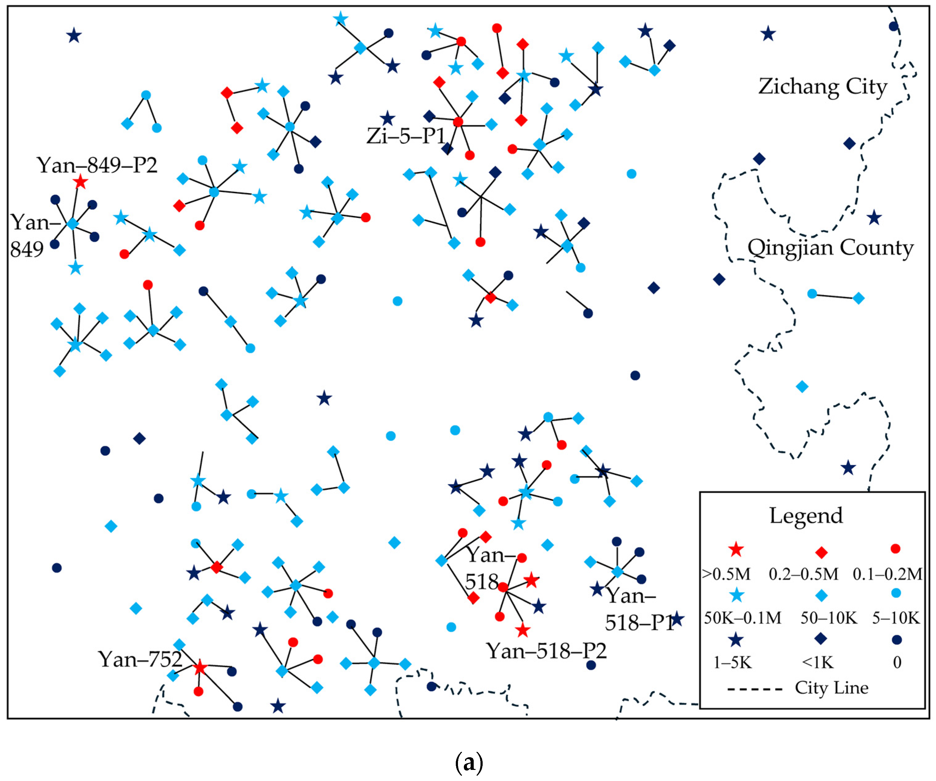
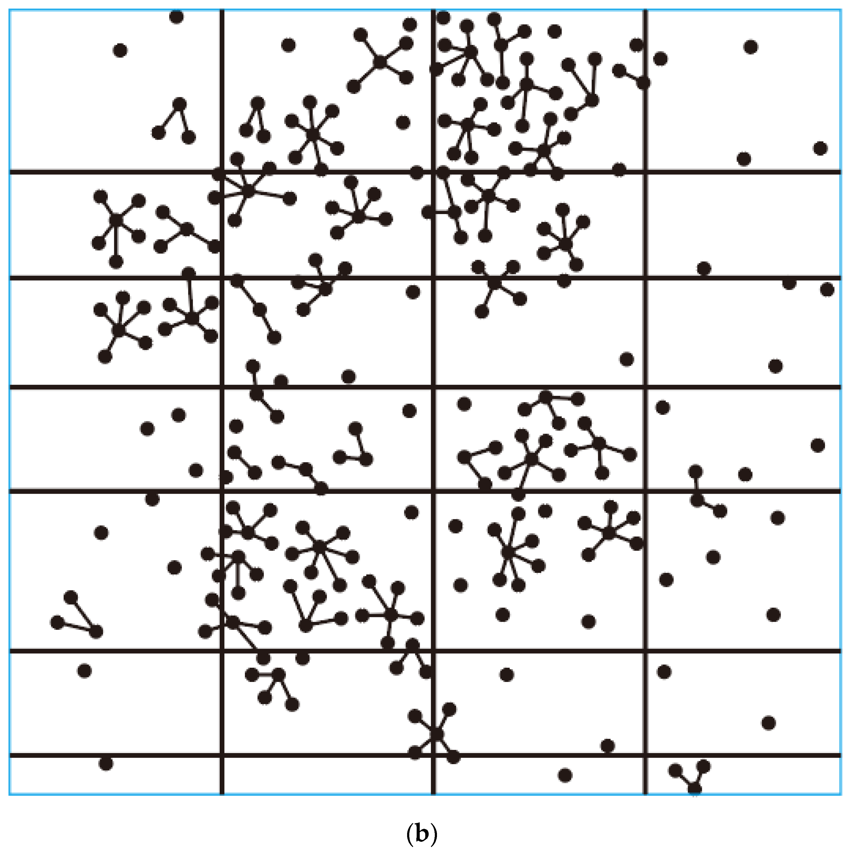
The following Figure 1 shows the information for the Zichang East block of tight sand gas reservoir in the Yan’an Gas Field. Figure 1a is the well layout and a partial distribution map of production rate of the existing wells. The red star symbols represent the locations of wells of the highest-production rate, the black dot symbols represent the locations of wells of the lowest-production rates, and other symbols represent wells with levels of production rate between the two extremes. Figure 1b is the plane view of distribution of the 2D seismic lines, where the black lines represent locations of seismic lines. The spacing between the seismic lines is 2 to 4 km. The dashed rectangular area highlights the Y849 well platform which will be used as an example for the detailed analysis of natural fractures in the subsequent sections. This spacing of 2 to 4 km is popular in existing practice. This value is reasonable for simulation of orogeny process in the region where there is no big fault and the top of formation is rather flat. For regions with complicated fault systems, this value may be too coarse to simulate orogeny process.

Figure 1. Information for the target Zichang East tight-sand gas block: (a) well distribution along with well production rates. (b) distribution of the 2D seismic survey line.

Table 2 provides the data on daily production rate for the 7 wells selected (shown in Figure 1). In the Figure 1 legend, M represents million m³/d, and K represents thousand m³/d. These wells are distributed across different areas of the target block. Among them, the Y849-P2 well is the one with highest gas production rate which has a value exceeding 910,000 m³/d, while Y849, which is the well with the lowest production rate, has a value of 23,647 m³/d. The Zi-5-P1 well produces 133,231 m³/d of gas. Some wells, after fracturing, communicate with water-bearing layers and produce a certain amount of water. Table 3 also includes information on the gas production rate as well as water production rate for each well, to indicate the development of natural fractures in the area.

Table 2. Production rate of selected 7 typical wells.

Serial Number	Well Name	Production Rate/m3/d	Water Production Rate/m3/d
1	Yan849-P2	914,750	5.7
3	Yan518-P2	783,789	15.33
4	Yan518-1	518,576	0
5	Yan518	430,450	2.214
6	Zi5-P1	133,231	27
7	Yan849	23,647	0

Table 3. Results of FMI measurements of natural fractures.

Layer Name	MD/m	Fracture Type	Inc/°	AZM/°
Shiqianfeng	1775.1	Natural Frac	40.3	146.4~326.4
Shiqianfeng	1832.9	Natural Frac	87.8	331.6~151.6
Shiqianfeng	1849.9	Natural Frac	82.3	169.7~349.7
Shiqianfeng	1850.5	Natural Frac	85	157.5~337.5
Shiqianfeng	1865.0	Natural Frac	38.2	144.4~321.1
Shiqianfeng	1867.3	Natural Frac	88.1	148.2~328.2
Shiqianfeng	1869.6	Natural Frac	87.6	143.2~323.2

Gas and water production from individual wells depend not only on natural fractures but also on fracture propagation induced by hydraulic fracturing and the resulting induced fractures [19,20]. However, hydraulically induced fractures develop on the basis of pre-existing natural fractures: the more developed the natural fracture network, the more effective the induced fracture system. Considering both aspects, it can be concluded that the degree of natural fracture development is directly and positively correlated with gas productivity of a well [20]. In another words, although gas production is influenced by hydraulic fracturing, induced fractures generally propagate along pre-existing natural fractures. Therefore, data of production rate provide indirect but meaningful constraints on damage variable as index of natural fracture development.

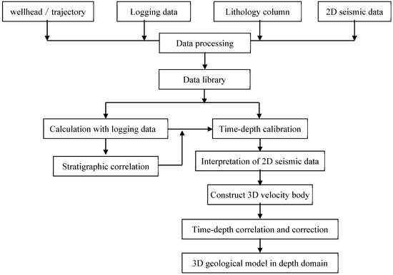
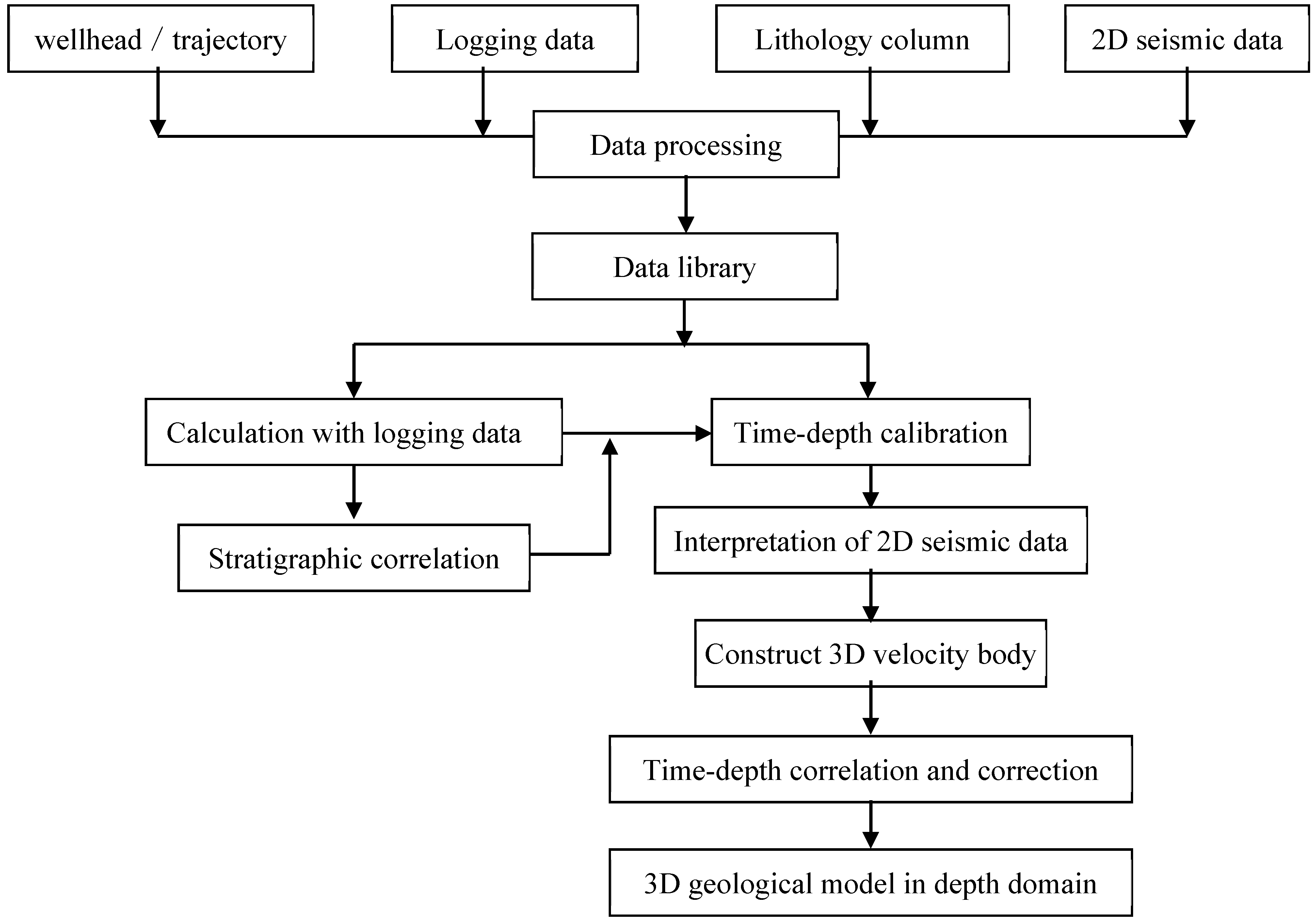
The 3D block model in this paper is established based on sets of 2D seismic data and well logging stratigraphic information. Figure 2 illustrates the corresponding workflow for establishing 3D model with sets of 2D seismic data as input. The more drilling, logging, and well logging data are collected from existing wells, the higher the accuracy of the constructed block geological model.

Figure 2. Flowchart for building 3D geological model with 2D seismic data and drilling data.

There are two key factors that affect the resultant model’s accuracy. The first is the density and quality of the 2D seismic lines: the denser and more accurate the seismic lines, the more accurate the resulting quasi-3D model will be. The second factor is the amount of available well sonic logging data and mud logging data: these data are used to calibrate the value of the wave propagation velocity $V_0$ for each stratum in the time–to-depth calibration step shown in Figure 2. More accurate velocity parameters lead to higher-fidelity 3D geological and finite-element models after subsequent time–depth conversion.

During the time–depth correction process, stratigraphic depths at well locations obtained from time–depth conversion are calibrated using well drilling and mud-logging horizon information. These calibrated depths are then used to adjust the positions of stratigraphic surfaces within the 3D geological model.

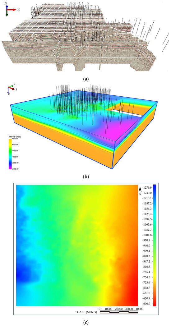
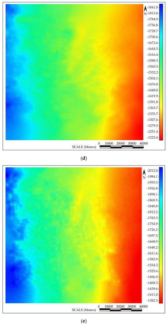
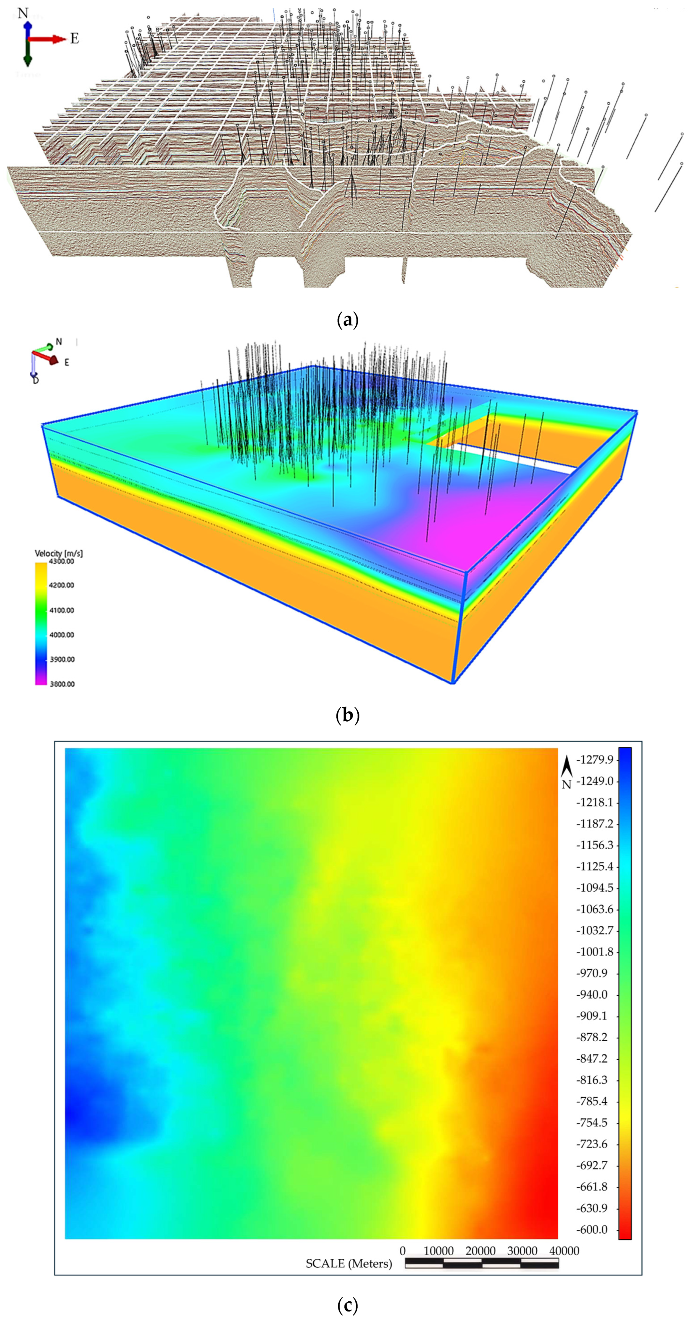
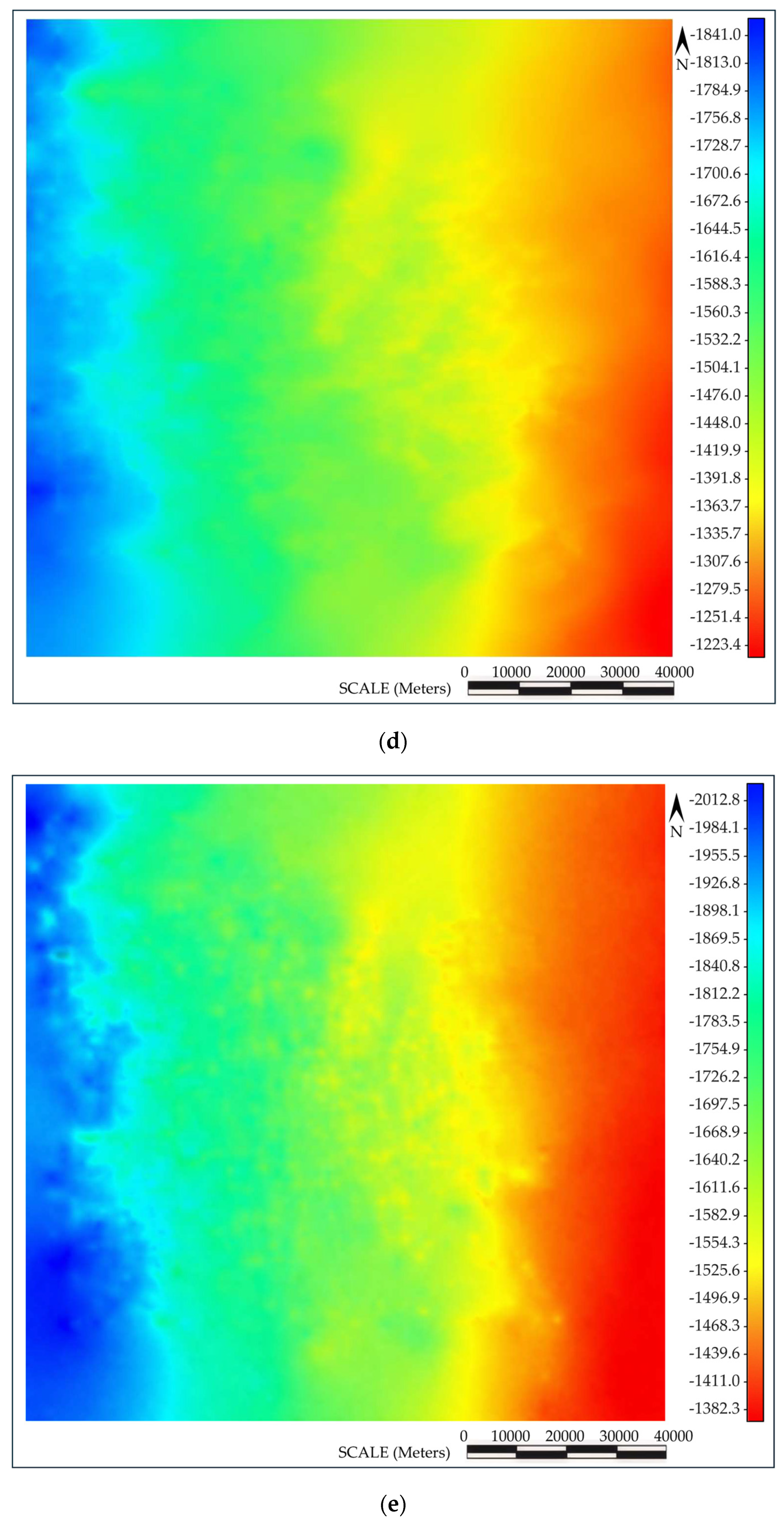
Figure 3 shows the geological model of the target block. Figure 3a is the 3D interpretation of the set of 2D seismic lines. The scope of the region is about 70 km in width and 85 km length. The black lines in Figure 3a,b represent the well trajectory. In Figure 3c–e, red and black symbols show the location of existing wells along with their names.

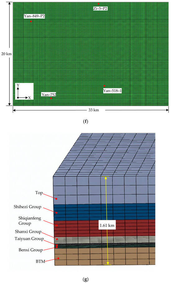
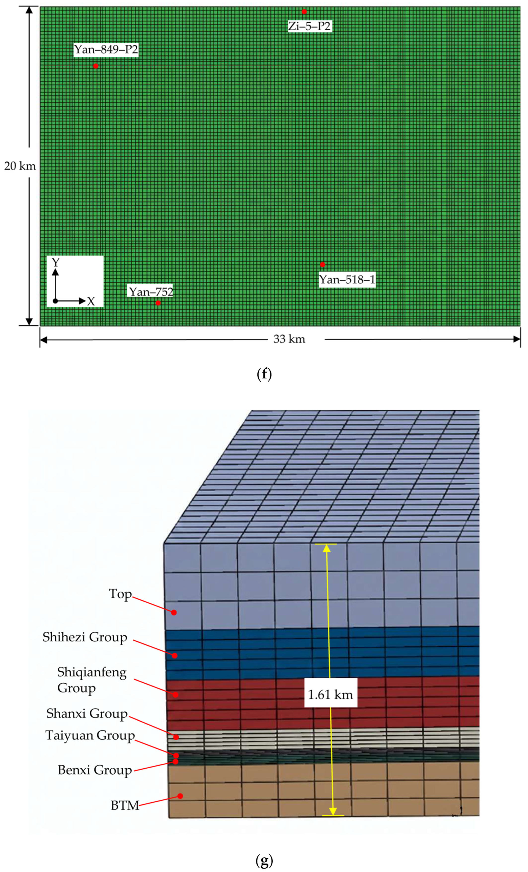
Figure 3. From sets of 2D seismic data to 3D geological model and its grid: (a) 3D interpretation of 2D seismic survey lines; (b) 3D velocity body; (c) formation top of ShiQianFeng; (d) top of ShanXi; (e) formation bottom of BenXi; (f) plane view of the 3D geological model; (g) zoomed view of mesh and formation layers.

Figure 3b is the 3D velocity model obtained by extrapolating and interpolating the set of 2D seismic lines given in Figure 3a.

Figure 3c is the planar view of the 3D geological model obtained after time–depth conversion and meshing. This model is only a part of the region shown in Figure 3b. The 3D model has a length of 33 km and a width of 20 km. The red dots in Figure 3c represent the locations of the four known wells which have high-production rate: Y849-P2, Y752, Y518-1, and Zi-5-P1.

Figure 3d is a zoomed view of the geological model’s grid and explanation of the stratigraphic layering, with the total model thickness being 1.61 km.

The model is based on sets of 2D seismic data integrated with well logging stratigraphic information for time–depth conversion and horizon calibration, resulting in a 3D geological model, with a total of 865,954 grid cells. The basal layer of the model is set as the basement stratum, with the Benxi Formation coal seam above it, followed by the Taiyuan Formation of tight sand, and then the Shanxi Formation of tight sand above that. The Shanxi Formation is the target layer for this calculation of natural fractures.

2.3. Analysis of Orogenic Movements and Measured Information of Natural Fractures

2.3.1. Analysis of Orogenic Movements

He et al. [21] provides a detailed analysis of the tectonic evolution of the Ordos Basin. The Shanxi Formation in the Zichang Block belongs to the Permian System and is characterized by coastal plain facies tight sandstone lithofacies. During the Permian, the eastern margin of the basin experienced the opening of an aulacogen, corresponding to the Hercynian tectonic cycle. The depositional framework is characterized by “east-west zonation and north–south extension”, resulting in reservoir bodies distributed as north-south-trending belts.

During the subsequent Triassic, the strata were affected by compressional tectonism associated with the Indosinian cycle of the Lvliang uplift. Thereafter, the region experienced additional tectonic events, including the Yanshanian cycle.

Based on preliminary trial calculations, the simulated distribution of damage zones obtained with a tectonic compression azimuth of N15°E shows the closest agreement with the natural fracture distribution inferred from the spatial distribution of high-production wells.

2.3.2. Measured Information of Natural Fractures

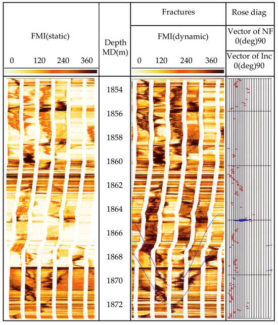
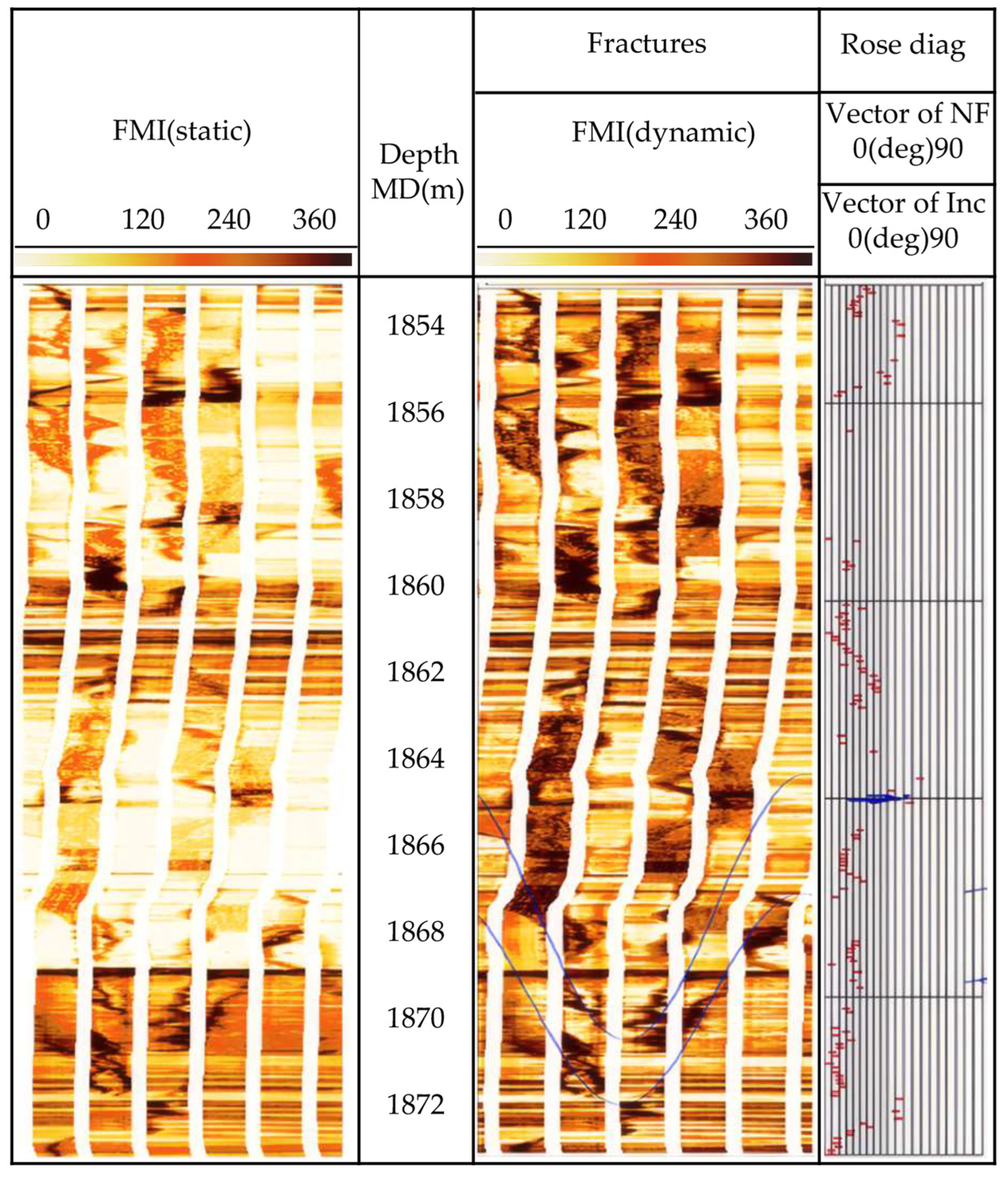
Formation Micro Scanner Image (FMI) measurement was made to the natural fractures on the borehole surface of Well Y1516 in the target block. Figure 4 shows that there are 3 fracture sets in this well section between depth 1854 m to 1972 m. Table 4 lists results of FMI measurements of natural fractures for this section.

Figure 4. FMI measurements of natural fractures of Y1516 well.

Table 4. Values of parameters of rock mechanics properties.

Layer Name	Rock Type	E/GPa	CS/MPa	ρ/g/cm3
ShiQianFeng	Tight sand	14	6	2.4
ShiHeZi	Tight sand	12	6	2.4
ShanXi	Tight sand	18	6	2.4
TaiYuan	Tight sand	25	8	2.4
BenXi	Tight sand	16	6	2.5
MaJiaGou	Carbonate	45	10	2.6

It is seen in Table 3 that most of the natural fractures in the reservoir are high-angle fractures with inclination angles exceeding 80°, while some are inclined fractures with inclination angles around 40°.

2.4. 1D Geomechanical Analysis of Typical Wells

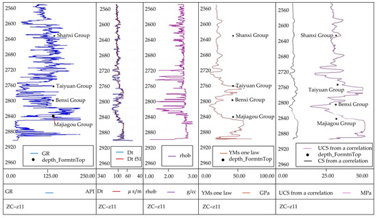
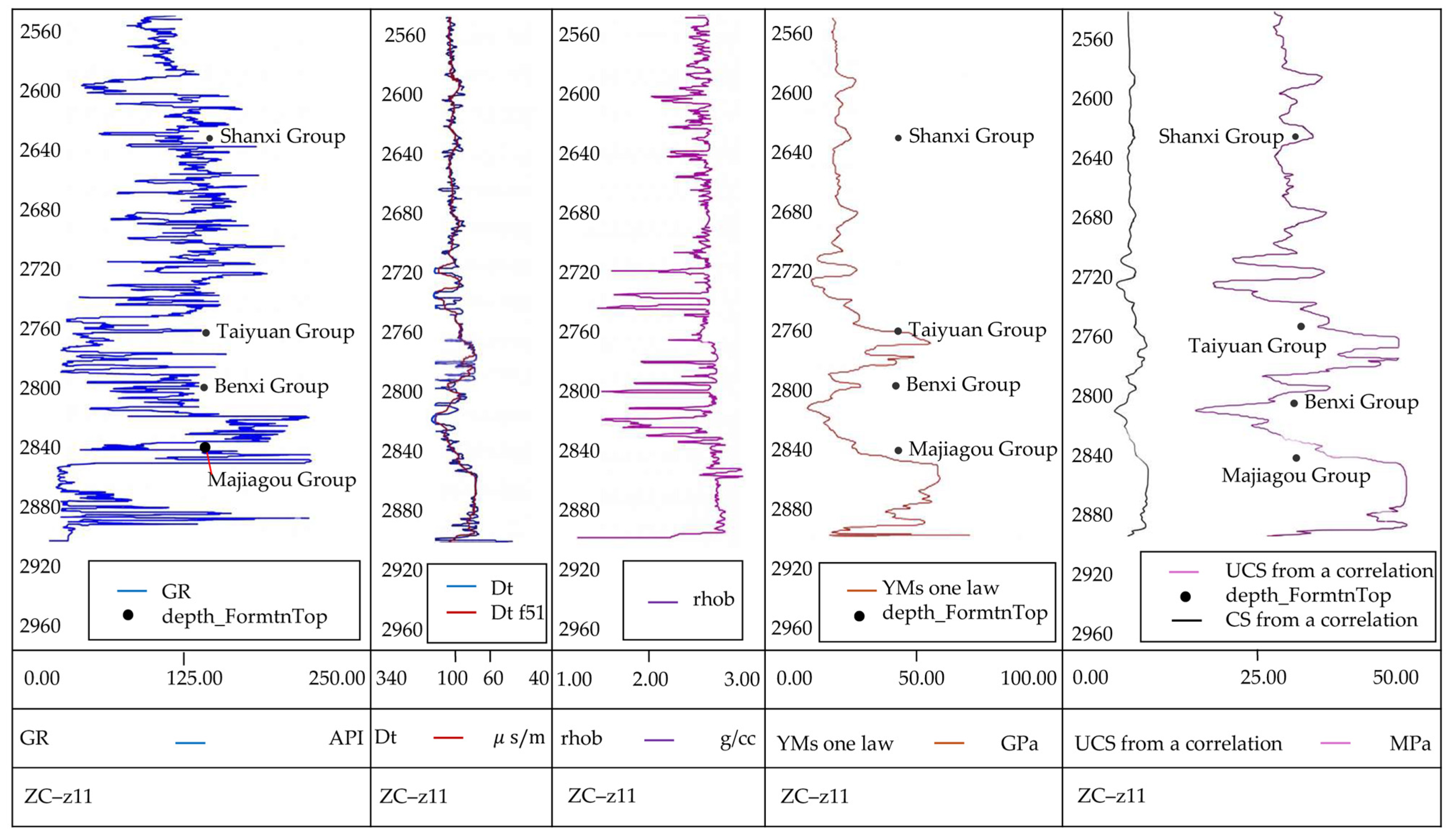
The purpose of 1D geomechanical analysis of typical wells is to derive values of parameters of mechanical properties of the rock from well logging curves and further use them as input data for the subsequent 3D finite element model. These parameters include Young’s modulus $E$, cohesion strength (CS), rock density, and others. Figure 5 shows the logging curves of Well Z11 and the single-well geomechanical analysis results calculated based on these data. The rightmost column presents the cohesion strength and uniaxial compressive strength curves. The software Drillworks/Predict 20.0.0 was used for these calculations.

Figure 5. Logging data of Z11 well and results of 1D geomechanics analysis.

Values of parameters of the rock mechanical property obtained from the analysis are listed in Table 4. These values of parameters are averaged values of parameters over each formation. Therefore, properties of formations are regarded as uniform.

2.5. Finite Element Model of the Target Block

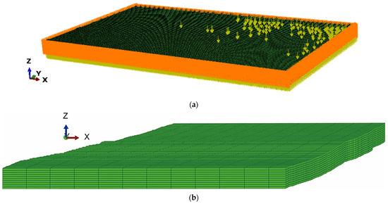
The scope and layers included in the Finite Element model are shown in previous Figure 3. Figure 6 shows the mesh of the finite element model of the target block. The boundary conditions are defined such that the four laterals and the bottom surfaces are constrained with zero normal displacement, while the top surface is free (see Figure 6a). The applied loads include the orogenic movement displacement and the gravitational load. The yellow arrow in Figure 6a is the symbol of gravity load to each element of the model. Non-zero-displacement constraints will be applied as orogenic movement after the step of calculation of initial geostress field. As the formation has not yet been deposited above the top layer of the model, there is no overburden load on the top of the model in Figure 6a. Figure 6b shows the mesh of the reservoir layers Shanxi Group and Taiyuan Group. Although it is rather flat, there is waving variation in the depth on the top of the Shanxi Group.

Figure 6. Finite element model: (a) load and boundary conditions, (b) mesh of the reservoir layers.

The model contains a total of 865,954 elements and uses 3D 8-node reduced-integration isoparametric solid elements (C3D8R), with a total of 907,200 nodes.

3. Results

Numerical Results of Natural Fracture Distribution and Their Comparison with the Distribution of Quantity of Well Production Rate

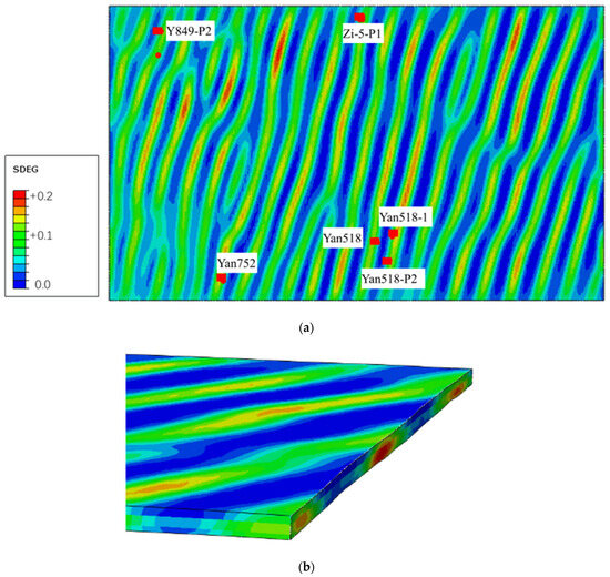
The large-scale commercial software Simulia/Abaqus 2025 was used as the platform toolset for solving aforementioned problem. Through a set of user subroutines, the model parameters of CDM listed in Table 1 and Table 2 were incorporated into the material model library of the software. Numerical calculations were then performed. Figure 7a shows the numerical solution of the contour of damage variable SDEG obtained from simulation of orogenic movement, presenting a map of distribution of natural fractures at the top of the Shanxi Formation. In Figure 7, red color indicates locations with the highest density of natural fracture as expressed by the damage variable SDEG, while blue color indicates locations with no natural fractures. As shown in Figure 7, natural fractures represented by zones of higher value of damage variable SDEG exhibit a narrow, banded distribution.

Figure 7. Contour of numerical results of damage variable SDEG under orogeny loading: (a) contour of SDEG on the top of Shanxi Formation; (b) partial 3D contour of SDEG with the view seeing from the right end of the reservoir formations.

The red symbols in Figure 7 represent locations of the wellhead and bottom of high-production wells. For vertical wells, the well’s bottom coincides with the wellhead and is therefore shown as a single red symbol. Figure 7b shows the partial 3D contour of SDEG with the view seeing from the right end of the reservoir formations shown in Figure 7a.

Figure 7b shows a 3D view of SDEG contour, with a cross-sectional view presented at its right end. It is seen in Figure 7b that the zones of natural fractures within Shanxi Formation and Taiyuan Formation are connected to each other. This corresponds to the vertical fractures obtained by FMI measurement. Table 5 has listed the daily production rate of selected 7 typical wells along with the maximum value of SDEG along the trajectory of these 7 wells. It basically follows the rule that the higher the value of damage variable SDEG, the higher the production rate will be.

Table 5. Comparison between production rate of selected wells with values of SDEG on their locations.

No.	Well Name	Daily Gas Production Rate/m3/d	Daily Water Production Rate/m3/d	Values of Damage Variable SDEG at Well Locations
1	Y849-P2	914,750	5.7	0.17
2	Y752	625,923	2.1	0.18
3	Y518-P2	783,789	15.33	0.19
4	Y518-1	518,576	0	0.19
5	Y518	430,450	2.214	0.15
6	Zi-5-P1	133,231	27	0.13
7	Y849	23,647	0	0.10

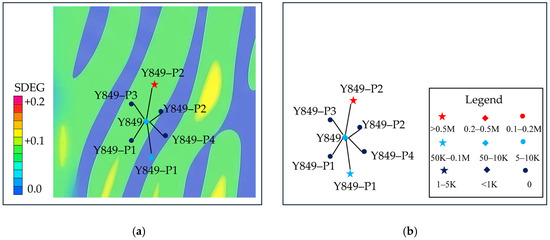
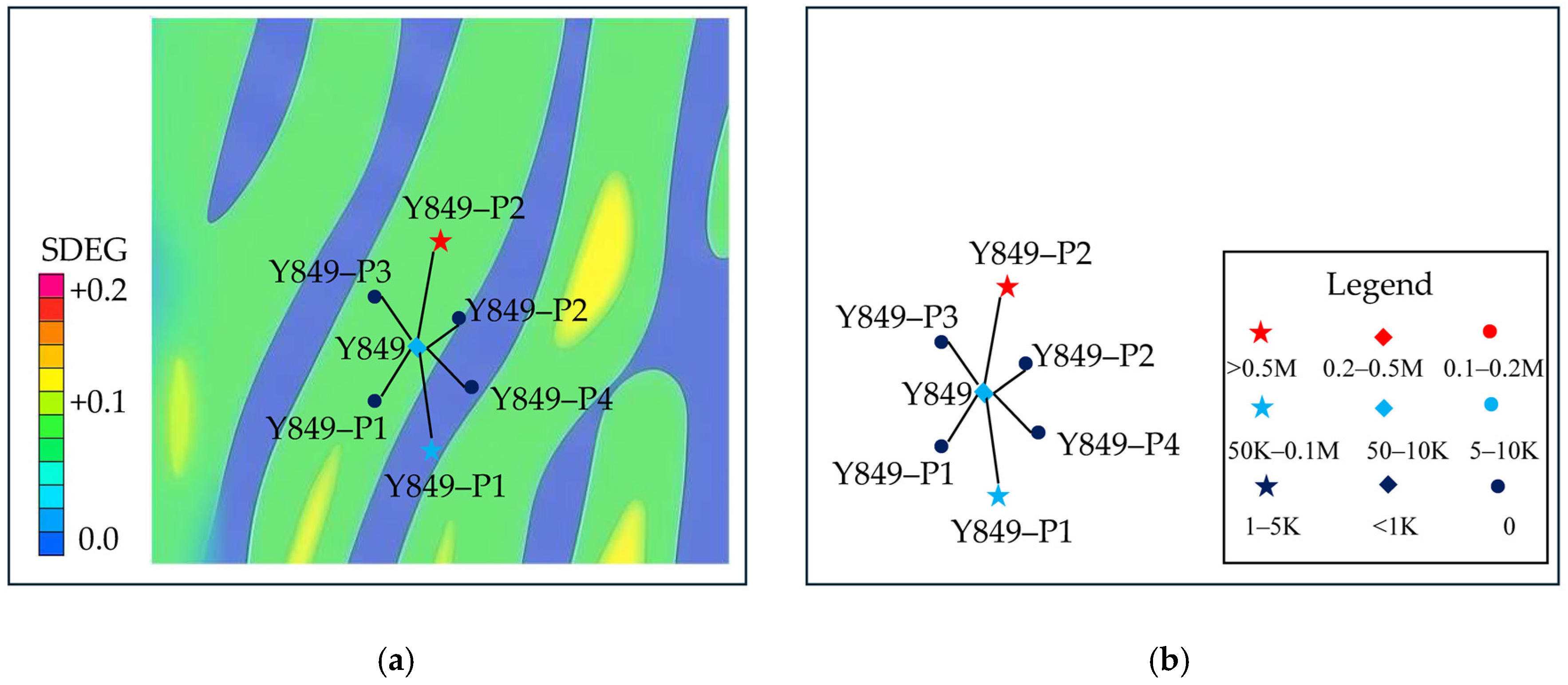
Figure 8a shows a superimposed comparison between the numerical contour map of the damage variable SDEG (Figure 7) around the Y849 well platform and relevant part of Figure 1, and Figure 8b shows the map of well locations along with their production rate (Figure 1). The values of damage variable SDEG represent natural fracture intensity.

Figure 8. Platform of Y849 well: zoomed view of contour of SDEG for this region along with the location distribution and production rate of wells (overlap for comparison purpose): (a) contour of SDEG around the region of Y849 wells; (b) daily production rate of the 849 wells.

The contour map in Figure 8a indicates that value of damage variable SDEG at the location of the high-production well Y849-P2 is significantly higher than those at other wells with value in the range of >0.5M m³/d, indicating a higher degree of natural fracture development. Correspondingly, its daily gas production rate is markedly greater than that of the other wells. In addition, the 1000 m horizontal well section of Y849-P2 also contributes to its high production rate.

Well Y849-P1 also has a 1000 m horizontal well section, but half of its trajectory goes through regions of lower values of SDEG which is of lower natural fracture intensity. Consequently, its production rate is lower than that of Y849-P2 and with values in the range of 50k~0.1M m³/d.

Well Y849-1 is located in a zone with relatively well-developed natural fractures, with values of damage variable SDEG slightly higher than those at Y849-P2. However, post-fracturing well testing encountered water production without gas, resulting in well shut-down and zero gas production. Well Y849-3 is located within the blue, low-damage region, representing poorly developed natural fractures, and shows no production. Wells Y849-2 and Y849-4 are situated along the margins of this fracture-poor region and are also non-productive. The vertical well Y849 is positioned between two moderately fractured (yellow) damage zones; its natural fracture intensity is relatively low, and its gas production is correspondingly lower than that of the surrounding wells Y849-P2 and Y849-P1, with a vale in the range of 10k~50k m³/d.

Based on these observations, the following conclusions are obtained:

(1)

Under normal conditions, gas production rate in the tight-sand gas reservoir exhibits a clear positive correlation with damage-derived natural fracture intensity: wells located in zones with higher values of damage variable SDEG show higher gas productivity.

(2)

In special cases, even in zones with well-developed natural fractures, stimulation-induced water production can significantly reduce gas output and may lead to well shut-down.

(3)

Wells located in low-damage (blue) regions, corresponding to poorly developed natural fractures, consistently exhibit very low gas productivity.

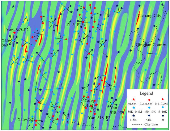
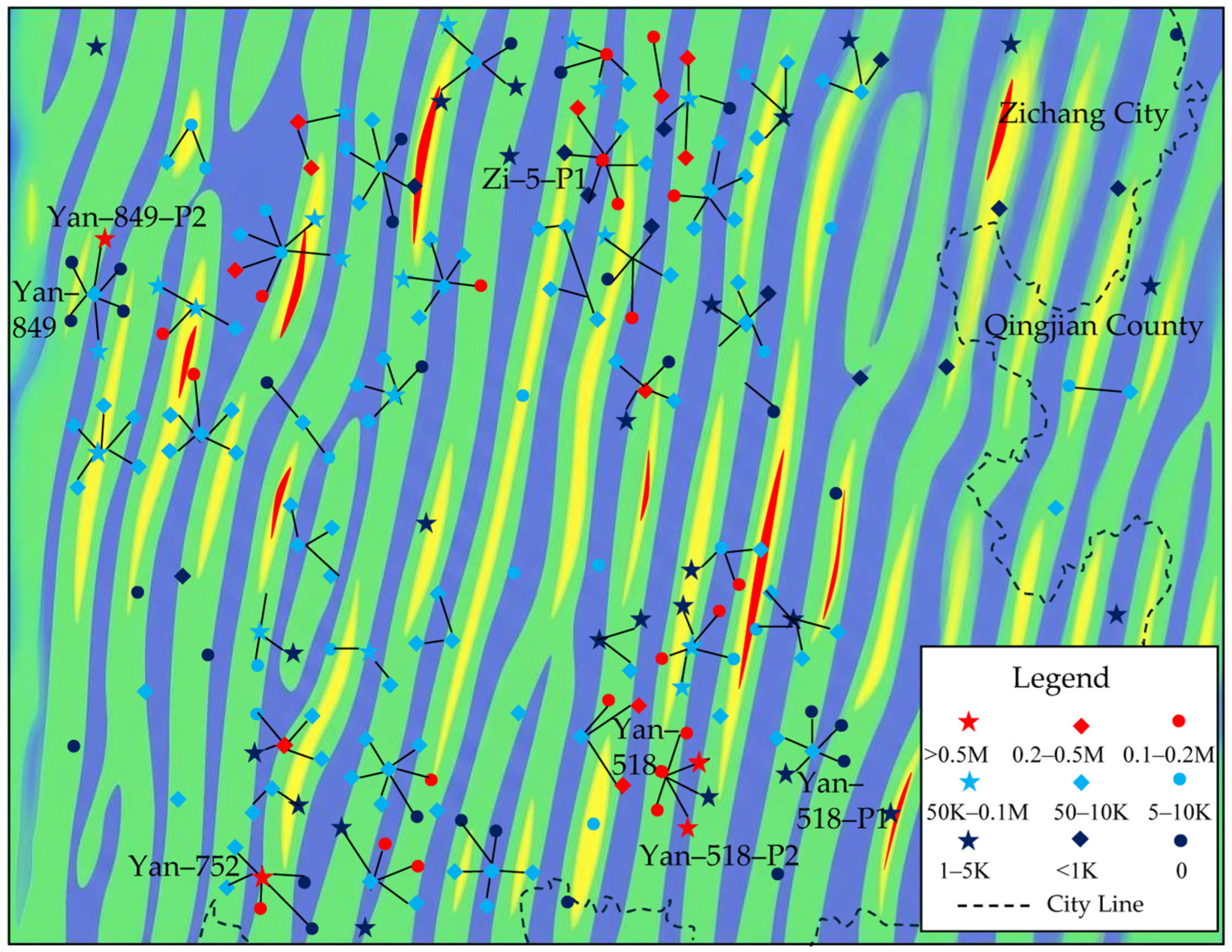
As shown in Figure 8, the well production distribution of the entire model block is superimposed on the damage-based natural fracture density contour map for comparative analysis. The results further validate the preceding conclusions:

(1)

Wells located in areas with high SDEG values (red zones) coincide precisely with the high-production wells identified in the observed data. This confirms a strong positive correlation between natural fracture density and well productivity, indicating reservoir sweet spots.

(2)

Wells situated in blue zones, where natural fractures are poorly developed, consistently exhibit low production, as indicated by the observed markers.

(3)

Low-production wells are also observed in several zones characterized by high values of damage variable SDEG. This is attributed to excessive injection rates during stimulation, which induced fracture communication with water-bearing layers, resulting in ineffective or non-productive wells. This indicates that for wells located in highly fractured reservoirs, hydraulic fracturing parameters—particularly pumping pressure and injection rate—must be carefully optimized to achieve effective stimulation.

The dashed outlines in Figure 9 delineate areas with high natural fracture density that have not yet been developed and therefore represent remaining reservoir sweet spots.

Figure 9. Overlap for comparison: contour of damage variable SDEG which represents natural fractures and the production rate of wells.

4. Discussion

This study applies a CDM model integrated with finite-element numerical simulation to establish a workflow for predicting the spatial distribution of natural fractures in tight-sand gas reservoirs. The method is applied to the Shanxi Formation in the Zichang East Block of the Yan’an Gas Field. The main conclusions are as follows:

(1)

Taking the Y849 well platform as an example, damage-derived fracture intensity is superimposed and compared with well locations and production data. A strong correspondence is observed: wells located in zones of high natural fracture density exhibit higher production, whereas wells in low-density zones show poor performance. In special cases, low-production wells occur in highly fractured zones due to stimulation-induced fracture communication with water-bearing intervals. These results demonstrate that the 3D natural fracture distribution obtained from CDM-based simulation of tectonic deformation satisfies engineering accuracy requirements for identifying remaining sweet spots.

(2)

The Y849 platform is located between two seismic lines. The results indicate that geological models interpolated between 2D seismic profiles are sufficiently accurate to meet engineering precision requirements.

(3)

Wells located in low-damage zones of the damage contour maps consistently exhibit very low production.

It should be noted that the natural fractures generated by tectonic deformation are structural fractures. Accordingly, the proposed method provides high accuracy in predicting tectonic natural fractures in tight-sand gas reservoirs but does not include weathering- or dissolution-related fractures. In addition, some natural fractures may become partially or fully cemented during later geological evolution and thus behave as inactive fractures. Such sealed fractures are not explicitly excluded from the numerical results and may locally reduce the correspondence between predicted fracture intensity and observed well productivity. Hydraulically induced fractures are assumed to preferentially propagate along pre-existing natural fractures.

The type of finite element proposed herein for simulating fractures generated by orogeny is an elastoplastic damage finite element model. For parameter identification, this study adopts a phenomenon-matching method to associate the locations of high-production-rate wells with the distribution of damage zones characterized by high fracture density. However, it is difficult to establish an explicit mathematical function as the objective for the parameter identification procedure.

Conversely, using AI-assisted computation, a non-structural surrogate model can be constructed between the model parameters and the elastoplastic damage finite element responses of the target block. A series of direct numerical simulations for orogeny-induced fracture evolution will be conducted to train the AI model, after which the optimal values of the model parameters can be determined.

5. Conclusions

(1)

In this study, the damage variable is interpreted as a proxy for natural fracture density, reflecting the cumulative effect of micro- and macro-scale fracture development under tectonic loading. CDM-based numerical modeling effectively predicts natural fractures in tight-sand gas reservoirs, particularly small-scale fractures and microfracture damage zones associated with very small or zero fault displacement that cannot be accurately resolved using conventional seismic interpretation.

(2)

Integration of 2D seismic data with drilling and mud-logging stratigraphic information enables construction of an accurate 3D geological and geomechanical model. Although only 2D seismic data are available, the integration of dense seismic profiles with well control ensures that the resulting 3D geological model achieves sufficient accuracy for engineering-scale simulations of mechanical behavior of the target block. This 2D-seismic-data-derived 3D geological model is not equivalent to the real 3D model obtained with 3D seismic data, but it is accurate enough for calculation of natural fractures by numerically simulating orogeny to generate natural fractures.

(3)

Spacing of 2D seismic lines is 2 to 4 km in this case. This value is reasonable for the case in Yan’an area because formation top here is relatively flat and there is no big fault. However, this value of spacing could be too big to obtain solutions of natural fractures with a reasonable accuracy when a target region is too complicated with existing big faults, etc.

References

- Wang, X.; Qiao, X.; Zhang, L.; Wang, Y.; Zhou, J.; Du, Y.; Cao, J.; Xin, C.; Song, J.; Yuan, F. Innovation and scale practice of key technologies for the exploration and development of tight sandstone gas reservoirs in Yan’an Gas Field of southeastern Ordos Basin. Nat. Gas Ind. 2022, 42, 102–113. [Google Scholar] [CrossRef]
- Du, J.; Zhu, G.; Li, Y.; Wu, P.; Gao, J.; Zhu, Y. Exploration and development challenges and technological countermeasures for tight sandstone gas reservoirs in Ordos basin margin: A case study of Linxing-Shenfu Gas Field. Nat. Gas Ind. 2022, 42, 114–124. [Google Scholar] [CrossRef]
- Huang, J.; Fan, L.; Zhang, Y. Geological characteristics of natural gas accumulation and exploration directions of the Cambrian System in the Ordos Basin. China Pet. Explor. 2025, 30, 98–110. [Google Scholar] [CrossRef]
- Jiang, L.; Wang, Q.; Ge, J.; Hu, Z. Identification and analysis of natural and induced fractures in cores: A case study of the Yanchang Formation, Ordos Basin. Chin. J. Geol. 2015, 50, 926–942. [Google Scholar] [CrossRef]
- Liao, H.; Liu, H.; Cui, Y.; Wang, R.; Li, Z.; Chen, D.; Liu, W. Fracture identification in metamorphic rocks based on conventional well logging. Mar. Geol. Quat. Geol. 2023, 43, 189–198. [Google Scholar] [CrossRef]
- Tong, H. Application of imaging well logging data in prediction of structural fracture. Nat. Gas Ind. 2006, 26, 58–61. [Google Scholar]
- Liu, Z.; Qu, S.; Sun, J.; Dong, N. Progress in seismic fracture characterization technology. Geophys. Prospect. Pet. 2012, 51, 191–198. [Google Scholar] [CrossRef]
- Ge, J.; Chen, C.; Liu, P.; Zhao, X.M.; Yi, Z.; Zhen, Y.; Zhang, A.; Tang, X.L. AI-driven seismic sedimentological characterization of shelf sand bodies: A case study of the Neogene Zhujiang Formation, Huizhou Sag, Pearl River Mouth Basin. Oil Gas Geol. 2025, 46, 860–875. [Google Scholar] [CrossRef]
- Shen, X.; Yang, L. Experiments and Theory of Damage Mechanics for Concrete; Science Press: Beijing, China, 2009; ISBN 9787030236777. [Google Scholar]
- Chen, M.; Zhang, C.; Canbulat, I.; Saydam, S. A DEM-DFN method for assessing mining-induced continuous fracturing and fracture connectivity in rock masses. Rock Mech. Rock Eng. 2025, 58, 12207–12230. [Google Scholar] [CrossRef]
- Tang, C.A.; Lin, P.; Wong, R.H.C.; Tsui, Y.; Tham, L.G. Numerical studies of the influence of microstructure on rock failure. Int. J. Rock Mech. Min. Sci. 2000, 37, 555–569. [Google Scholar] [CrossRef] [Scilit]
- Hampton, J.; Gutierrez, M.; Matzar, L. Microcrack damage observations near coalesced fractures using acoustic emission. Rock Mech. Rock Eng. 2019, 52, 3597–3608. [Google Scholar] [CrossRef] [Scilit]
- Zhou, H.W.; Wang, X.Y.; Zhang, L.; Zhong, J.C.; Wang, Z.H.; Rong, T.L. Permeability evolution of deep coal samples subjected to energy-based damage variable. J. Nat. Gas Sci. Eng. 2020, 73, 103070. [Google Scholar] [CrossRef] [Scilit]
- Vazic, B.; Bryant, E.C.; Bennett, K.C. Single-objective optimization for modeling elastoplastic damage of rock. Int. J. Rock Mech. Min. Sci. 2025, 186, 106034. [Google Scholar] [CrossRef] [Scilit]
- Gale, J.F.W.; Laubach, S.E.; Olson, J.E.; Eichhubl, P.; Fall, A. Natural fractures in shale: A review and new observations. AAPG Bull. 2014, 98, 2165–2216. [Google Scholar] [CrossRef] [Scilit]
- Zhao, G.; Ding, W.; Sun, Y.; Wang, X.; Tian, L.; Liu, J.; Shi, S.; Jiao, B.; Cui, L. Fracture development characteristics and controlling factors for reservoirs in the Lower Silurian Longmaxi Formation marine shale of the Sangzhi block, Hunan Province, China. J. Pet. Sci. Eng. 2020, 184, 106470. [Google Scholar] [CrossRef] [Scilit]
- Laubach, S.E.; Lamarche, J.; Gauthier, B.D.M.; Dunne, W.M.; Sanderson, D.J. Spatial arrangement of faults and opening-mode fractures. J. Struct. Geol. 2018, 108, 2–15. [Google Scholar] [CrossRef] [Scilit]
- Dassault Systèmes Simulia Corp. Abaqus User’s Manual, Vol. 2: Analysis (Version 2025). Vélizy-Villacoublay, France. 2025. Available online: https://www.3ds.com/support/documentation/ (accessed on 10 April 2026).
- Li, P.; Li, S.; Song, H.; Sun, X.D. Influence of natural fractures on hydraulic fracturing based on microseismic monitoring. In Proceedings of the Third China Petroleum Geophysical Academic Conference; Chinese Petroleum Society: Beijing, China, 2025; Volume IV, pp. 427–430. [Google Scholar] [CrossRef]
- Wang, T.; Zhao, H.; Yang, Z.; Zhang, S.; Ren, C. Influence of natural fractures on hydraulic fracturing effectiveness in shale reservoirs: A case study of the Qingshankou Formation, Gulong Sag, Songliao Basin. Oil Geophys. Prospect. 2025, 60, 213–224. [Google Scholar] [CrossRef]
- He, F.; Huang, L.; Jia, H.; Zhang, R.; Zhang, W.; Wang, C.; Li, X.W. Characteristics of strike-slip faults and their control on hydrocarbon accumulation in the Ordos Basin. Acta Geol. Sin. 2025, 99, 520–534. [Google Scholar] [CrossRef]
Disclaimer/Publisher’s Note: The statements, opinions and data contained in all publications are solely those of the individual author(s) and contributor(s) and not of MDPI and/or the editor(s). MDPI and/or the editor(s) disclaim responsibility for any injury to people or property resulting from any ideas, methods, instructions or products referred to in the content. |
© 2026 by the authors. Licensee MDPI, Basel, Switzerland. This article is an open access article distributed under the terms and conditions of the Creative Commons Attribution (CC BY) license.