


Abstract
Autonomous Underwater Vehicles (AUVs) play a crucial role in deep-sea exploration missions. In the complex and highly dynamic marine environment, it is essential for AUVs to possess robust fault diagnosis capabilities to enhance their operational safety. In the context of AUV fault diagnosis, closed-set recognition methods tend to misclassify unknown faults as known ones, which may lead to severe operational consequences. In order to enable AUVs to adapt to new and unknown deep-sea environments and effectively detect new unknown faults, this paper proposes an open-set AUV fault recognition method based on a Convolutional Neural Network (CNN). Firstly, the CNN is employed to extract high-level discriminative features from raw sensor data. Then, a committee consisting of multiple one-class SVMs (OC-SVMs) is constructed to determine whether the input sample belongs to a known category. Finally, the identified known samples are accurately classified via the designed classifier module. This method can effectively distinguish between known faults and unknown faults. To improve the recognition accuracy of the model, an attention mechanism is introduced. By learning to automatically assign weights to different feature channels, the model can focus on more important or relevant feature channels. Experiments based on the “Haizhe” dataset demonstrate that the proposed CNN-OC-SVM model exhibits superior performance in AUV fault diagnosis tasks compared with the state-of-the-art and traditional methods.
1. Introduction
Autonomous underwater vehicles (AUVs) have become key equipment in fields such as marine resource exploration and environmental monitoring due to their strong autonomy and wide coverage. With the increasing demand for deep-sea missions, the intelligence and reliable operation of AUVs have become crucial [1,2,3]. However, the actual marine environment is complex and ever-changing, and AUVs are prone to performance degradation or sudden failures due to long-term operation under multiple extreme environmental coupling effects such as high pressure, low temperature, and complex hydrodynamics [4]. AUVs should have the ability to identify faults and take appropriate measures to ensure their own safety, otherwise it may lead to mission interruption and data loss, and may even cause equipment damage, resulting in significant economic losses and safety hazards [5]. Consequently, investigating intelligent fault diagnosis methods capable of identifying multiple types of faults has become an urgent requirement for enhancing the autonomy and operational safety of AUVs, and also represents an important direction in the development of marine intelligent equipment technology [6].
In recent years, the intelligent fault diagnosis of AUVs has rapidly developed, relying on deep learning technology [7]. However, traditional diagnostic models are mostly built on static and closed datasets, which are difficult to adapt to the open and dynamic fault feature space faced by AUVs in actual marine environments [8]. With the development of AUV operation tasks towards deep sea and long endurance, the system complexity and environmental uncertainty continue to increase, and unknown fault modes also continue to appear [9]. When traditional diagnostic frameworks encounter novel fault features, they lack prior knowledge regarding such new faults and thus tend to misclassify them as known fault categories. Such misjudgments can induce AUVs to make erroneous response decisions, thereby giving rise to unpredictable risks and substantial losses [10].
In this context, an increasing number of studies have begun to focus on open-set fault diagnosis (OSFD) for AUVs (AUV-OSFD). The test set for open-set fault diagnosis includes unknown novel faults, and existing AUV open-set fault diagnosis methods are primarily categorized into three types: unknown detection-based OSFD Methods, incremental learning-based OSFD Methods, and open-set classification-based OSFD Methods. The OSFD method based on unknown detection first distinguishes between known and unknown patterns, then classifies the known patterns, primarily relying on distance metric methods and error reconstruction analysis. The OSFD method based on incremental learning extends the known fault scope by integrating new fault data through incremental learning on the basis of an existing closed-set model, mainly utilizing modular networks and incremental regularization. The OSFD method based on open-set classification directly constructs an end-to-end model capable of simultaneously achieving “known classification” and “unknown identification,” eliminating the need for a separate unknown detection module, and primarily employs techniques such as meta-learning and open-set deep learning [11].
Currently, research on OSFD based on the aforementioned methods has made certain progress. Palermo et al. [12] presented a novel unsupervised online method for detecting unanticipated faults in AUVs. The core idea is to analogize the multivariate time-series sensor data of an AUV as a document and treat data patterns under different operational states as vocabulary. An online Dirichlet Process (DP) topic model is applied to this framework. Li et al. [13] proposed the RM-MFKAN model, which leverages the Rainbow Memory framework to select and replay critical historical samples, enabling AUVs to continuously learn new faults without forgetting prior diagnostic knowledge through an enhanced KAN-based network. Wu et al. [14] constructed a meta-learning framework that is trained through a multitude of simulated diagnostic tasks. Each task simulates a few-shot open-set scenario, spanning from known faults to scenarios containing unknown faults.
To solve the problem that the AUV closed-set fault diagnosis model cannot effectively identify unknown faults, this paper proposes an OSFD method based on unknown detection. This study proposes a CNN-OC-SVM model based on the combination of CNN and one-class support vector machine (SVM). The model can combine the advantages of deep learning and SVM algorithms to distinguish between known and unknown faults, and make accurate judgments on known fault types. The main contributions are as follows:
- (1)
- This study presents a novel hybrid approach for AUV fault diagnosis that integrates deep learning with traditional machine learning. The method employs deep learning techniques to extract discriminative features from raw sensor data. These features are then processed by multiple one-class SVM models, each trained to find a minimum-volume hypersphere in the feature space that encapsulates most known normal-state feature points. The final diagnostic decision is made based on the voting results of these one-class SVM classifiers.
- (2)
- A feature extraction method that integrates an attention mechanism improves the quality of feature extraction by automatically learning important time regions.
- (3)
- Using the softmax algorithm as a known fault classifier, if the sample is accepted by at least one SVM, it is judged as a known class. The softmax classifier is used to determine the specific fault type of the known class sample.
- (4)
- The effectiveness of the CNN-OC-SVM model is validated on the “Haizhe” AUV benchmark dataset, where it achieves stronger multi-modal feature fusion capabilities.
2. Related Work
2.1. AUV Fault Diagnosis
In recent years, deep learning technology has been widely applied in the field of AUV intelligent fault diagnosis [15]. Ji et al. [16] employed a sequence convolutional neural network based on deep learning algorithms to learn the mapping patterns between state data and fault types, extracting both global and local features from the state data and classifying the extracted information into different fault types, thereby transforming the traditional two-stage diagnostic model into a single-stage diagnostic approach. To address the various interferences that complex marine environments may impose on signals, Wang et al. [17] proposed a semi-supervised interference suppression method based on a parallel hypergraph attention network-graph convolutional network for AUV thruster fault diagnosis. By constructing a dynamic hypergraph attention network based on the hypergraph convolutional network and integrating the hypergraph attention network with the graph convolutional network through a novel parallel connection strategy, the network can simultaneously learn both dynamic and static features of the input graph signals, effectively suppressing interference. In order to deal with the problem that propeller fault samples are very scarce and difficult to collect, and that traditional fault diagnosis faces the challenge of insufficient data, Du et al. [18] proposed a channel attention residual transfer learning model based on double loss nonlinear independent component estimation, aiming to solve the problem of small-sample fault diagnosis of AUVs through data amplification. Considering that the fault diagnosis model faces many uncertainties, ref. [19] proposed a deep belief rule base model with attribute reliability. In order to solve the problem of rule explosion, a gradient rising framework is established. The attribute reliability is evaluated by using the statistical calculation method of attribute credibility. The evidential reasoning is used as the model reasoning engine. Finally, the interpretable whale optimization algorithm is applied to optimize the model parameters. Xia et al. [20] introduced a deep learning-based fault diagnosis framework for autonomous underwater vehicles that incorporates an attention mechanism. By integrating a spatial attention module into the fault detection network, their approach captures semantic associations between monitoring variables and fault types, and subsequently derives fault identification results based on the analysis of these semantic relationships. However, although these studies have achieved good results in fault diagnosis of marine equipment, in practical application, if the AUV produces a new unknown fault, the model will recognize it as a known fault and cannot make an accurate decision.
2.2. Open-Set Fault Diagnosis
At present, the research on using deep neural network to solve the problem of open-set fault diagnosis is gradually carried out [21]. Zhou et al. [22] proposed a residual capsule network combined with tag mask weighted prototype learning, which can simultaneously identify unknown faults and composite faults. Li et al. [23] proposed an open-set fault diagnosis model that integrated fine-grained clustering and a rejection mechanism, which enhanced intra-class compactness through multi-scale feature extraction and a distance-based loss function, and constructed an unknown fault identification mechanism based on extreme value theory. Shan et al. [24] proposed an open-set fault diagnosis method for nuclear power plant time-series data, which utilized kernel density estimation (KDE) and an LSTM autoencoder to extract probability density features, and employed Elliptic Envelope models to effectively identify unknown faults. Wang et al. [25] proposed a cross-domain fault diagnosis method based on current signals and a dual-feature-driven siamese network (SN-CDFD), which extracted weak fault information by integrating global and local features and achieved iterative identification of unknown faults in open-set scenarios through a meta-learning-guided threshold mechanism. Yu et al. [26] and Wang et al. [27] proposed incremental learning fault diagnosis models, assuming that unknown faults emerge progressively. Zhuo et al. [28] introduced a zero-shot learning fault diagnosis model, where fault attributes serve as auxiliary information to guide the generative adversarial network in synthesizing minority-class or unknown fault samples.
While the aforementioned studies have achieved progress in open-set recognition, most of them focus on fault diagnosis for bearings and similar systems. Research on open-set fault diagnosis specifically for AUVs remains relatively scarce. Part of the research focuses on incorporating the detected unknown faults into the closed-set diagnosis system, rather than focusing on the identification of unknown faults. Some studies rely on the accurate attribute description of all fault types, but it is not guaranteed to synthesize effective unknown fault samples for training an open-set fault diagnosis model under actual conditions. In order to solve the problem of open-set fault diagnosis for AUVs, a CNN-OC-SVM model is developed in this paper, which can recognize unknown categories and classify known categories.
3. Methodology
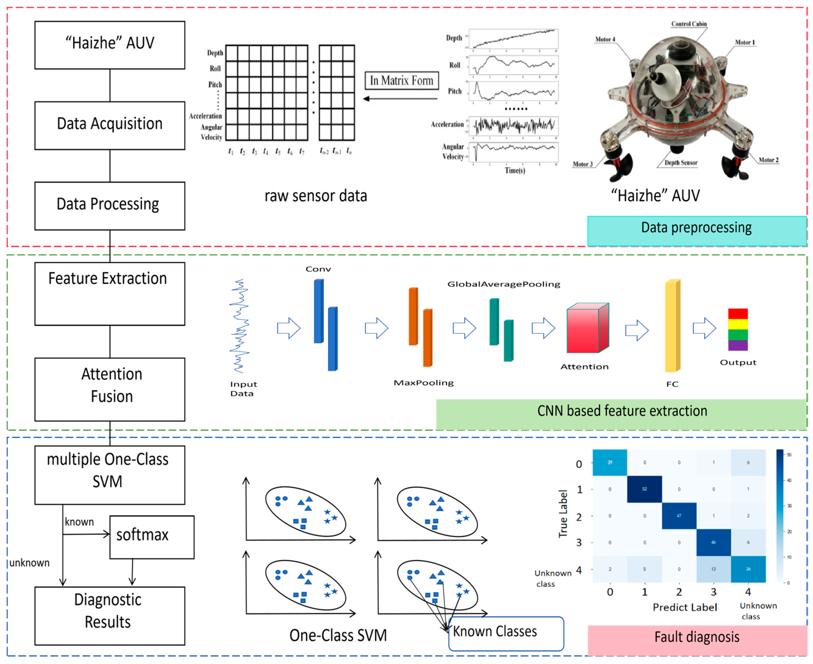
This research proposes the CNN-OC-SVM model, which is based on the collaborative combination of CNN and multiple OC-SVM, as shown in Figure 1. The model uses deep learning technology to analyze the data characteristics, and through multiple OC-SVM voting to divide known categories and unknown categories, it can effectively identify new faults.
Figure 1.
The structure of AUV fault diagnosis using CNN-OC-SVM model.
In the feature extraction stage, local temporal features are extracted through the convolution layer. An attention mechanism is introduced after the convolutional layer, which generates the attention weight of each time step through the full connection layer and softmax function, so as to fuse the features of key time steps. This attention mechanism enables the model to adaptively focus on the most discriminative part of the input sequence, suppress noise interference, and finally generate a more differentiated normalized feature vector for classification.
A separate one-class SVM model is trained for each known class. During inference, we compute the decision score for each SVM, which represents the signed distance from the sample to the boundary. For each class, we set a class-specific threshold based on the distribution of decision scores from training samples. A sample is considered “accepted” by a class only when its decision score is greater than the class-specific threshold. If a sample is accepted by at least one class, it is classified as known, with the final label determined by the class achieving the highest decision score; otherwise, it is rejected as unknown.
3.1. CNN Model
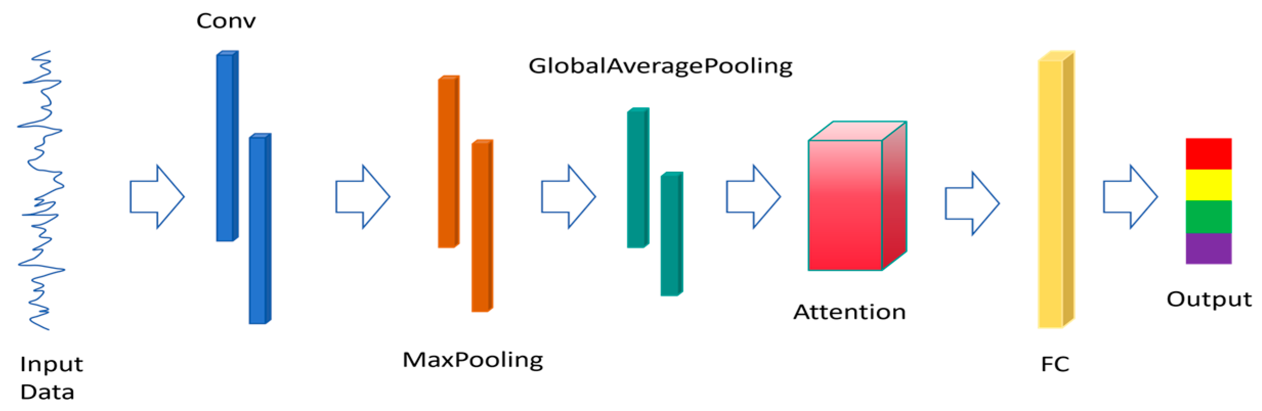
At present, the research on AUV fault diagnosis based on convolutional neural network (CNN) is still in the stage of theoretical exploration, and there have been some related attempts [29,30,31]. Deep learning network can mine and extract deeper feature information from fault data and effectively improve the accuracy of fault diagnosis. In this work, the original state data of the AUV serves as input. A one-dimensional convolutional neural network is employed to capture local temporal features, and an attention mechanism is introduced to refine the quality of the extracted features. The network structure is shown in Figure 2.
Figure 2.
The network structure.
3.1.1. Convolutional Feature Extraction Module
1D-CNN is a convolutional neural network that utilizes one-dimensional convolution to extract features from one-dimensional time series while preserving temporal characteristics [32,33,34]. In the AUV fault diagnosis task, the original sensor data is multiple one-dimensional time series data, which meets the input standard of 1D-CNN.
In order to ensure the consistency of network input, the original sensor data is preprocessed. The time step length of the single-pick time series is 196, and each time step contains 12 feature dimensions. The input layer of the model receives the time series data with the dimension of (196, 12). First, it enters the one-dimensional convolution feature extraction module. The core of this module consists of multiple one-dimensional convolutional kernels, which encode local features at each time step and its neighboring time steps through sliding convolution operations. The convolution operation is formulated as follows:
In the formula, denotes the weight matrix of the convolutional kernel, where k is the temporal size of the kernel, F is the input feature dimension, and represents the number of output channels of the convolution. The symbol ∗ denotes the one-dimensional convolution operation, and is the bias term of the convolutional layer. σ(·) is the activation function, with the Rectified Linear Unit (ReLU) being commonly employed. Its mathematical expression is given as follows:
The output of the convolutional layer, , is fed into a batch normalization layer to mitigate internal covariate shift. The operation is formulated as follows:
In the formula, and denote the mean and variance of the current batch B, respectively; ϵ is an infinitesimal constant to prevent division by zero; γ and β are the learnable scaling and shifting parameters; ⊙ represents element-wise multiplication; and is the output of the batch normalization layer.
Then, maxpooling1d continuously reduces the size of data space through downsampling operation, which reduces the computational complexity and improves the generalization ability of the model. In this study, downsampling is performed in the time dimension with a step size of 2. The specific operation is to take the maximum value in each adjacent window with a length of 2. This operation not only reduces the time sequence length of the feature graph to half of the original, realizes the compression and abstraction of features, but also endows the model with a certain degree of time translation invariance. The specific formula is as follows:
where is the output of the maximum pooling layer. Then, the dropout layer randomly sets the output of some neurons in this layer to zero with a certain probability, and its output is expressed as . This efficient regularization technology prevents the model from over fitting the training data by preventing the complex cooperative adaptation between neurons, so as to improve the generalization ability of the model.
3.1.2. Attention Weighting Module
In order to make the model have the ability to identify and handle uncertainty when encountering unknown class samples, this study proposes to introduce an uncertainty channel attention mechanism into the model. The two-way attention mechanism is used to simultaneously learn the deterministic and uncertain characteristics of the channel, and the attention weight is adaptively adjusted based on the uncertainty.
Firstly, the mean and maximum values of channels are extracted respectively through global average pooling and maximum pooling, and the difference between them is calculated as the quantitative index of channel change amplitude. The specific calculation formula is as follows:
In the formulas, denotes the channel mean, T is the time step length, represents the channel maximum, and indicates the maximum variation in each channel along the temporal dimension. A larger value of reflects more intense temporal fluctuation of the corresponding channel feature, implying higher uncertainty.
Then, the certainty weight and uncertainty weight are generated respectively based on the mean value and change amplitude, and the formula is as follows:
In the equations, and are the learnable weight matrices of the deterministic branch; and are the learnable weight matrices of the uncertainty branch; denotes the sigmoid activation function; and and represent the deterministic weight and uncertainty weight, respectively.
Next, calculate the characteristic uncertainty and normalize it. The formula is as follows:
In the equations, is the learnable weight matrix for uncertainty estimation; U denotes the feature uncertainty; is a function employed for smooth uncertainty estimation, ensuring non-negative outputs; and represents the uncertainty score, where 0 indicates complete certainty and 1 corresponds to high uncertainty.
Then, the uncertainty perception fusion is performed, the uncertainty penalty term is calculated, and the final attention weight is updated. The formula is as follows:
In the equations, denotes the penalty term, is the hyperparameter controlling the degree of influence of the uncertainty attention; represents element-wise multiplication; and is the final attention weight.
Finally, complete the attention weighting and calculate the output of the feature. The formula is as follows:
In the equation, denotes the learnable scalar residual weight. is the weighted eigenvalue and is the output of the attention module.
3.1.3. Fully Connected Classification Module
Following the attention module, a global pooling operation is applied, compressing the temporal features into channel-wise statistics to facilitate processing by fully connected layers; the output after global pooling is denoted as XGAP. The fully connected layers non-linearly map the features into a high-dimensional discriminative space, with ReLU activation functions incorporated to enhance the model’s nonlinear fitting capability. Then the features are normalized and regularized by batch normalization, dropout and L2 normalization to maximize the robustness of the features.
First, the full connection layer nonlinearly maps the low-dimensional aggregate features to the high-dimensional discriminant feature space. The specific calculation formula is as follows:
Among them, and are the weight matrix and bias term of the fully connected layer, respectively; denotes the ReLU activation function; and represents the output of the fully connected layer.
Next, the batch normalization is implemented in the same way as Formulas (3) and (4), and the output is recorded as . The output of the dropout layer is obtained by randomly deactivating the output of the normalization layer, which is recorded as . Finally, the L2 norm feature normalization of is performed, and the result is expressed as . After this mandatory feature standardization operation, the features are projected onto the unit hypersphere. The similarity between samples is only determined by the angle of the feature vector, not the module length, which can effectively suppress the interference caused by the scale difference in the feature values. The normalized features can make the category probability distribution of subsequent Softmax output smoother and more reasonable.
3.1.4. Classified Output Layer
Map the normalized feature vector to the classification space and output the probability distribution of each category. The calculation formula is
In the formula, and represent the weight matrix and bias term of the classification layer, respectively; is the model’s predicted probability vector, where each element represents the probability of the sample belonging to the corresponding category. Finally, the category with the highest probability is taken as the final prediction result, i.e.,
In the formula, represents the model’s prediction result.
3.1.5. Model Training Strategy
The model uses the most commonly used Adam adaptive learning rate optimizer in the deep learning time series classification task. By combining the momentum gradient descent and adaptive learning rate, it can effectively deal with the sparse gradient. The model uses sparse classification cross-entropy loss for end-to-end training, and the calculation formula is as follows:
where represents the loss value, N is the batch size (number of samples in the batch), is the true label of the -th sample, and is the model’s predicted probability that the sample belongs to its true label.
3.2. One-Class SVM
Traditional multi-class SVM needs to use all class samples for training at the same time, while one-class SVM (OC-SVM) is designed for open-set scenarios. It only needs known class samples in the training phase, and it can judge whether the test samples belong to known or unknown classes in the reasoning phase.
3.2.1. Working Principle
OC-SVM is a classical unsupervised anomaly detection and open-set classification algorithm. Its core assumption is that the known class samples form a compact cluster in the feature space, which can be separated from the anomaly samples by hypersphere or hyperplane. The optimization goal of the algorithm is to find an optimal decision boundary, so that
- (1)
- Known-class samples should be maximally contained within the boundary;
- (2)
- Any region lying outside the boundary is considered to belong to anomalous or unknown categories;
- (3)
- Compactness of the boundary is to be optimized for better generalization performance.
Through Lagrangian dual transformation, the original optimization problem is converted into a dual problem, which can be described as follows: For the known-class sample set (where d is the feature dimension), a kernel function is introduced to achieve nonlinear boundary learning, namely
In the formula, represents the Lagrange multiplier corresponding to the i-th sample; denotes the kernel function; is the anomaly ratio parameter; n is the number of samples in the training set; and represents the upper bound for .
The commonly used kernel functions include linear kernel, polynomial kernel, radial basis function (RBF) kernel, etc. In this research, the RBF kernel is selected. It is a kernel function with strong locality, which can map a sample to a higher dimensional space and has strong nonlinear mapping ability. The calculation formula is as follows:
In the formula, is the parameter that controls the smoothness of the kernel function.
Extract features from samples of known classes in the training set as the input of OC-SVM, train OC-SVM for each class, and calculate the decision threshold of this class. The threshold calculation formula is as follows:
In the equation, is the feature vector of the test sample, and is the decision score for sample , representing the position of sample relative to the hypersphere. If , it will receive one vote; otherwise, it will not receive any vote.
3.2.2. Workflow
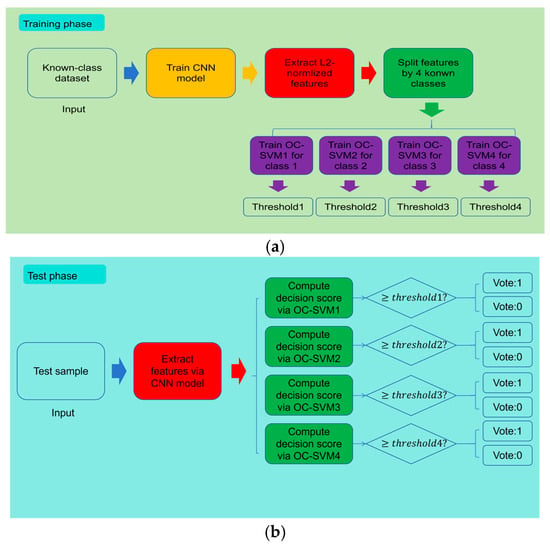
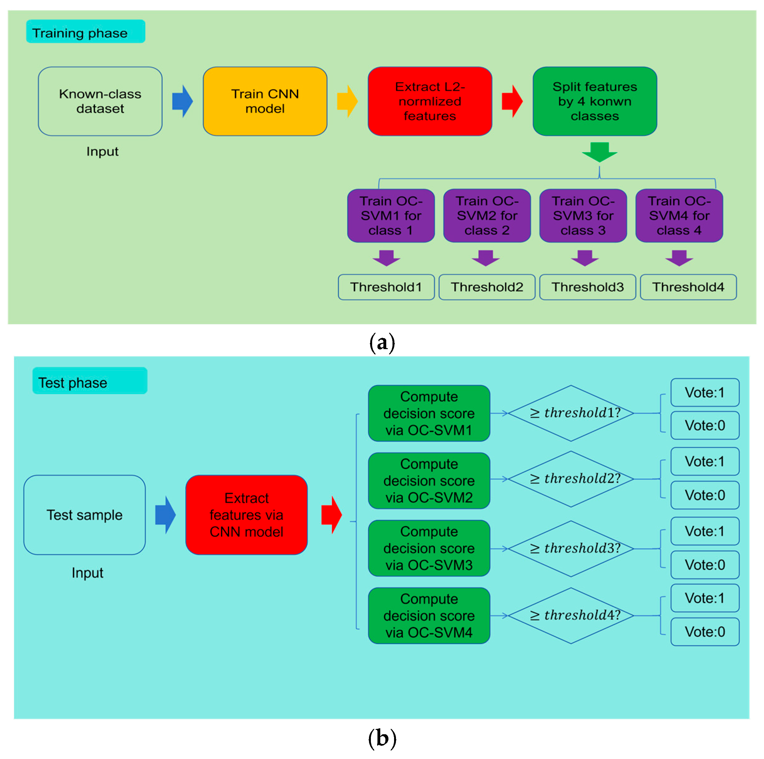
In this research, four classes of known samples were used to form a known-class dataset, which served as the input to the model. The training and test processes are illustrated in Figure 3.
Figure 3.
Workflow of the CNN-OC-SVM. (a) Training phase. (b) Inference phase.
A CNN was trained to extract feature vectors, and these vectors were correspondingly divided into four sets. A OC-SVM was trained for each class, and a decision threshold was computed for each one. During the inference phase, feature values of test samples were extracted using the CNN model. Each OC-SVM then calculated a decision value based on its corresponding feature vector and compared it with its respective threshold. If the decision value was not less than the threshold, a vote of 1 was assigned; otherwise, a vote of 0 was assigned.
4. Experimental Study
4.1. AUV Dataset
This study employs a fault dataset collected from navigation experiments conducted with Zhejiang University’s “Haizhe” AUV [35]. The dataset is available at https://data.mendeley.com/datasets/7rp2pmr6mx/1 (accessed on 1 June 2025), which is a complete open-source dataset. This AUV is a compact, self-developed underwater operation platform equipped with a propulsion motor, depth sensors, and a control module. The name and description of each column is listed as in Table 1.
Table 1.
Sensor data of “Haizhe” AUV dataset.
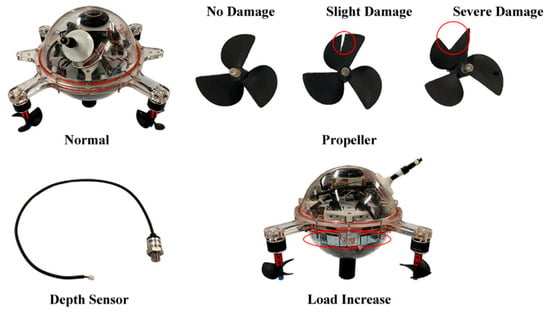
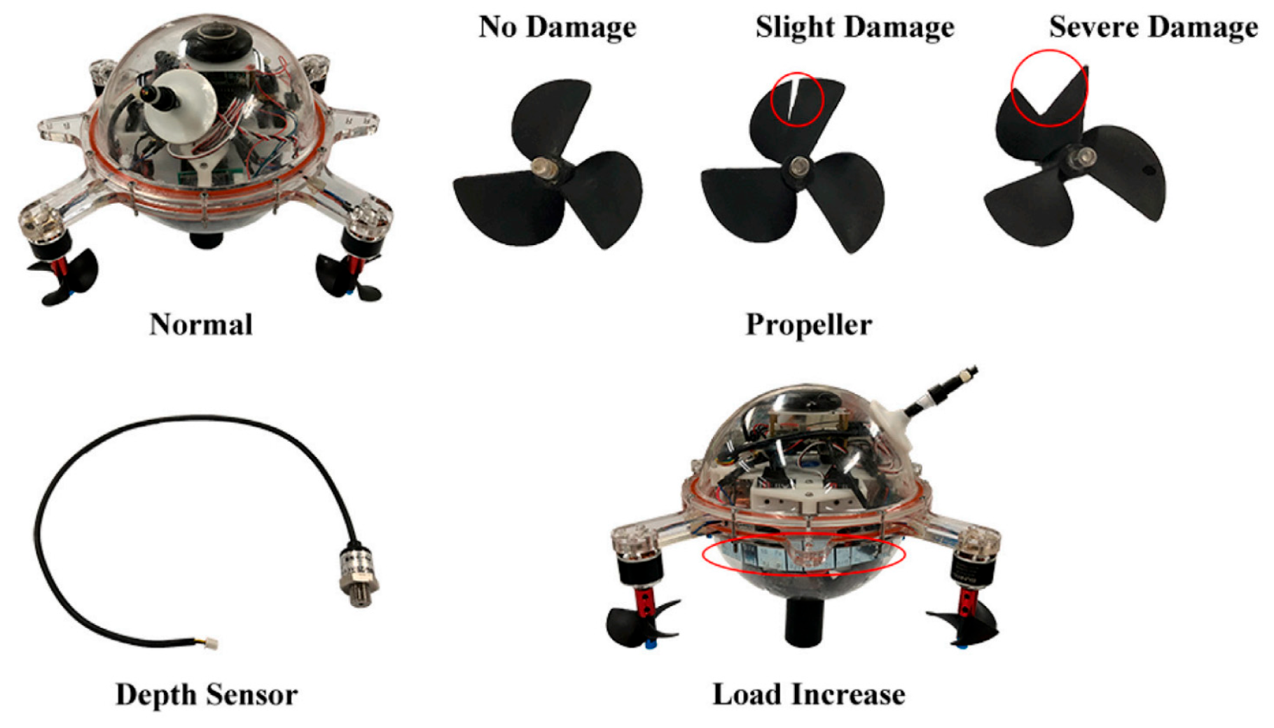
During the data collection process, the vehicle was equipped with both depth sensors and inertial measurement units (IMU). Each experiment simulated a single-fault condition lasting 10 to 20 s. The “Haizhe” platform exhibited five operational states: normal operation, depth sensor failure, increased payload, minor propeller damage, and severe propeller damage. The fault labeling and dataset sample statistics are presented in Table 2, and the details of the fault settings are shown in Figure 4.
Table 2.
Details of “Haizhe” dataset.
Figure 4.
Fault types setting for ‘Haizhe’. The red circles indicate the fault locations.
Considering the limited contribution of some sensor data to fault diagnosis and computational cost concerns, we selected 12 sensor modalities from the “Haizhe” dataset—specifically excluding time and pwm1–4 from Table 1—which collectively encode the AUV’s operational states across varying environmental conditions. Each sensor channel is processed by sequence length standardization and feature standardization. First, by truncating redundant data or copying the end value of the sequence, the data length is adjusted to 196 data points to ensure dimensional consistency while maintaining data continuity; Then, Z-score standardization is applied to normalize the data to have zero mean and unit variance, which is essential for stabilizing the training of deep learning models and ensuring the effectiveness of distance-based methods such as one-class SVM and OpenMax.
4.2. Experimental Setup
The experiment used the open-source deep learning library TensorFlow developed by the Google Brain team, and was performed on an Intel (R) Core (TM) i7-14650HX configuration CPU@2.20 (Intel, Santa Clara, CA, USA). Conduct experiments on a computer with GHz and 16 GB memory.
To maintain experimental rigor, we standardized hyperparameters across all evaluations using the “Haizhe” dataset, as detailed in Table 3. Specifically, the configuration employed included learning rate, batch size, and epoch number, as described below.
Table 3.
Hyperparameter settings for model training.
4.3. Experiment Process
The experiment uses the training set and test set in Table 2. During the training process, the data of 4 categories in the training set is used as the training sample, and during the testing process, the data of 5 categories in the test set is used as the test sample. Therefore, the test results will include 4 labels (0–3) of known classes and 1 unknown fault label (4). A total of 80% of all known class samples are randomly selected as training samples, the remaining 20% are used as test samples, and 50% of the unknown samples are added to the test set. Taking PressureGain_constant as the unknown class as an example, the experimental content and results are presented.
4.4. Comparative Experiment
To experimentally analyze the effectiveness of the algorithm proposed in this study, we conducted multiple sets of validation experiments using the “Haizhe” dataset. Each set of experiments was conducted 10 times, and the evaluation metrics were calculated as the average of the 10 runs. Several evaluation metrics are selected to measure model performance, namely
- (1)
- Known Class Accuracy: the percentage of correctly classified samples among all known class samples;
- (2)
- Unknown Class Accuracy: the percentage of correctly classified samples among all unknown class samples;
- (3)
- Weighted Accuracy: an accuracy metric calculated by combining the proportions of known and unknown class samples;
- (4)
- AUROC: the area under the Receiver Operating Characteristic (ROC) curve;
- (5)
- AUPR: the area under the Precision–Recall (PR) curve.
4.4.1. Ablation Study on Feature Extractor
Firstly, an ablation experiment was conducted on the feature extractor. To demonstrate the rationality and necessity of the CNN model architecture, comparisons were made among the CNN-BiLSTM model, the LSTM-only model, the CNN-unidirectional LSTM combined model, and the BiLSTM-only model. Table 4 lists two sets of experimental parameters. The results for the first parameter set are shown in Table 5, while the results for the second set are presented in Table 6.
Table 4.
Key parameters.
Table 5.
Results of the Feature Ablation Experiment 1.
Table 6.
Results of the Feature Ablation Experiment 2.
Experimental results demonstrate that the CNN model outperforms other models across multiple evaluation metrics, confirming its effectiveness.
4.4.2. Ablation Study on Attention Mechanism
Secondly, an ablation study on the attention mechanism was conducted. The uncertainty weight is a core hyperparameter in the uncertainty-aware channel attention mechanism. It precisely controls the model’s suppression strength on unstable features through a fusion formula combining the uncertainty penalty term and the uncertainty branch contribution term. When this value is relatively small, the model adopts a conservative strategy, assigning higher weights to all channels. This allows full utilization of all feature information but makes the model more susceptible to noise interference. When the value is moderate, the model achieves an optimal balance, effectively suppressing noise interference from unstable channels while preserving discriminative information from stable channels. This enhances the clustering of known class features and effectively pushes unknown class features toward the decision boundary periphery. When the value is too large, the model becomes overly aggressive, and excessive penalization of fluctuating features may lead to the loss of useful information. Although the open-set detection capability is further improved, it comes at the cost of classification accuracy for known classes.
In this study, we perform grid search over the uncertainty parameter within the range of [0.1, 0.2, 0.3, 0.4, 0.5, 0.6, 0.7, 0.8, 0.9, 1.0], selecting the optimal value based on the weighted accuracy on the validation set. The operating results under different parameters are shown in Table 7.
Table 7.
Uncertainty parameter search results.
Based on the experimental results, we selected 0.6 as the optimal hyperparameter for the uncertainty parameter.
To verify the effectiveness of the attention mechanism, we conducted multiple experiments. The experiment compared four models: Model 1: a baseline CNN model without any attention mechanism; Model 2: the CNN model incorporating a self-attention mechanism; Model 3: the CNN model incorporating a temporal-attention mechanism; Model 4: the CNN model incorporating a uncertainty-channel-attention mechanism. Meanwhile, under the experimental condition of the aforementioned training-to-test set split ratio (8:2), we added comparative experiments with other split ratios. With PressureGain_constant and AddWeight as the unknown classes respectively, the experimental results of the four models under different partitioning ratios are shown in Table 8.
Table 8.
Results of the Attention Ablation Experiment.
Based on a comprehensive comparison of multiple evaluation metrics, the CNN model integrated with the uncertainty-channel-attention mechanism (Model 4) exhibits superior performance. Specifically, under the 7:3 split ratio, it achieves an 8% improvement in weighted accuracy compared to the baseline model.
4.4.3. Comparative Experiment on Open-Set Recognition
Finally, a comparative experiment on open-set recognition was conducted. We added comparative experiments with the typical open-set recognition algorithm OpenMax. Open-set Max pooling (OpenMax) is an algorithm designed for open-set recognition. It uses extreme value theory to model the extreme value of the tail of the feature distribution of a known class, so as to estimate the probability that the sample belongs to an unknown class. In this study, the enhanced version of OpenMax is used, and its working principle is as follows: first, it calculates the class center in the feature space for each known class, and calculates the distance from the sample to various centers by using Euclidean distance, cosine distance or Mahalanobis distance, respectively; then, the tail sample with the largest distance is selected for each category, and the extreme value distribution of the fitting feature is used to model the decision boundary of each category. In the prediction stage, the system calculates the cumulative probability score of the sample belonging to a certain class based on the fitting Weibull distribution and integrates three types of uncertainty based on the extreme value theory: distance uncertainty, relative distance proportion uncertainty and entropy uncertainty of softmax output, so as to correct the original activation value and reduce the score of the higher uncertainty category. Finally, by adding an additional activation value of “unknown class” and applying Softmax with temperature parameters, the OpenMax probability distribution containing the probability of unknown class is generated. When the probability of unknown class exceeds the preset fixed threshold, the sample is determined as an unknown class, so as to achieve accurate recognition in the open-set environment.
The preset fixed threshold is a super parameter which has a great impact on the performance of OpenMax algorithm. In order to find the best threshold, we set an optional parameter set, namely Threshold_OpenMax = [0.1, 0.2, 0.3, 0.4, 0.5]. The accuracy under different thresholds is shown in Table 9.
Table 9.
Comparison of recognition accuracy of OpenMax.
Each threshold was tested in 10 experimental trials, and the average of the test results was taken, where the weight for calculating the weighted accuracy accounted for the number of known and unknown class samples. The experimental results indicate that 0.2 is the optimal threshold for the current experimental scenario. This parameter was consequently adopted for all subsequent comparative experiments.
To demonstrate the effectiveness of the OC-SVM-based algorithm, the following comparative experiments were performed: Model 1: The CNN-OC-SVM model proposed in this paper. Model 2: Features were extracted using CNN, with the OC-SVM algorithm removed, utilizing only Softmax. Model 3: Replacing Softmax in Model 2 with OpenMax. We employed the leave-one-class-out method, setting each of the five categories as the unknown category in turn. The order of the unknown categories was: Normal, PropellerDamage_bad, PropellerDamage_slight, AddWeight, and PressureGain_constant. The statistical results of 10 experiments for the three models under each setting are shown in Table 10.
Table 10.
Experimental results of open-set recognition methods comparison.
Through feature extraction ablation experiments, we selected CNN as the base model for open-set fault recognition of underwater vehicles. In the attention mechanism ablation experiments, we introduced an uncertainty attention mechanism and determined the optimal hyperparameter for the uncertainty weight via grid search. Based on this, we compared the performance of models with no attention mechanism, with other attention mechanisms, and with the uncertainty attention mechanism. The results showed that the introduction of the uncertainty attention mechanism led to an improvement in weighted accuracy. Finally, we validated the performance of CNN-OC-SVM against the CNN-SoftMax and OpenMax algorithms under different unknown class settings. The average weighted accuracies of the three algorithms were 0.84, 0.63, and 0.73, respectively, with CNN-OC-SVM outperforming the other two algorithms by 33% and 15%. Experimental results demonstrate that the CNN-OC-SVM algorithm significantly outperforms the comparison algorithms in terms of both accuracy and F1 score, confirming its effectiveness and superiority in open-set recognition tasks.
5. Conclusions
During underwater operations, autonomous underwater vehicles (AUVs) may encounter novel and unknown faults, which traditional closed-set recognition methods tend to misclassify as known fault types. To address this issue, this paper proposes a fault diagnosis method based on CNN-OC-SVM. This method first utilizes a convolutional neural network (CNN) to extract representative features from raw multimodal sensor data and continuously learns the mapping between these features and fault categories. Subsequently, the features extracted by the CNN are used to train multiple one-class support vector machines (OC-SVMs) to compute decision thresholds for each known class. During testing, the CNN extracts feature vectors from input data, and each OC-SVM calculates a decision score for the corresponding feature. If the score exceeds its threshold, a vote of 1 is assigned; otherwise, a vote of 0 is assigned. If the total number of votes is greater than or equal to 1, the sample is classified as known, and the CNN model outputs its specific category; otherwise, it is classified as unknown. Multiple comparative experiments were conducted using the “haizhe” dataset. Feature ablation experiments demonstrate that the standalone CNN architecture achieves notable performance, while attention mechanism ablation experiments show that incorporating a channel attention mechanism further improves model evaluation metrics.
Author Contributions
Conceptualization, L.D.; Methodology, L.D.; Software, L.D.; Validation, L.D.; Formal analysis, L.D.; Investigation, Y.H.; Resources, L.D.; Data curation, Y.H.; writing—original draft preparation, L.D. All authors have read and agreed to the published version of the manuscript.
Funding
This research received no external funding.
Institutional Review Board Statement
Not applicable.
Informed Consent Statement
Not applicable.
Data Availability Statement
The original contributions presented in this study are included in the article. Further inquiries can be directed to the corresponding author.
Conflicts of Interest
The authors declare no conflicts of interest.
References
- Wynn, R.B.; Huvenne, V.A.I.; Le Bas, T.P.; Murton, B.J.; Connelly, D.P.; Bett, B.J.; Ruhl, H.A.; Morris, K.J.; Peakall, J.; Parsons, D.R.; et al. Autonomous Underwater Vehicles (AUVs): Their past, present and future contributions to the advancement of marine geoscience. Mar. Geol. 2014, 352, 451–468. [Google Scholar] [CrossRef] [Scilit]
- Vangi, M.; Topini, E.; Liverani, G.; Topini, A.; Ridolfi, A.; Allotta, B. Design, Development, and Testing of an Innovative Autonomous Underwater Reconfigurable Vehicle for Versatile Applications. IEEE J. Ocean. Eng. 2025, 50, 509–526. [Google Scholar] [CrossRef] [Scilit]
- Vallicrosa, G.; Fumas, M.J.; Huber, F.; Ridao, P. Sparus II AUV as a Sensor Suite for Underwater Archaeology: Falconera Cave Experiments. In Proceedings of the 2020 IEEE/OES Autonomous Underwater Vehicles Symposium (AUV), St. John’s, NL, Canada, 30 September–2 October 2020; IEEE: Piscataway, NJ, USA, 2020; pp. 1–5. [Google Scholar] [CrossRef] [Scilit]
- Fourlas, G.K.; Karras, G.C. A Survey on Fault Diagnosis and Fault-Tolerant Control Methods for Unmanned Aerial Vehicles. Machines 2021, 9, 197. [Google Scholar] [CrossRef] [Scilit]
- Mai, J.; Luo, Z.; Ge, G.; Zhang, G.; He, W. A Fault Diagnosis Method for Autonomous Underwater Vehicles Based on Online Extended Belief Rule Base With Dynamic Rule Reduction. IEEE Access 2024, 12, 165407–165424. [Google Scholar] [CrossRef] [Scilit]
- Dong, L.; Huo, Y. Research on Fault Diagnosis Method for Autonomous Underwater Vehicles Based on Improved LSTM Under Data Missing Conditions. Appl. Sci. 2025, 15, 11570. [Google Scholar] [CrossRef] [Scilit]
- Said, N.; Mansouri, M.; Al Hmouz, R.; Khedher, A. Deep Learning Techniques for Fault Diagnosis in Interconnected Systems: A Comprehensive Review and Future Directions. Appl. Sci. 2025, 15, 6263. [Google Scholar] [CrossRef] [Scilit]
- Ma, S.; Leng, J.; Zheng, P.; Chen, Z.; Li, B.; Li, W.; Liu, Q.; Chen, X. A digital twin-assisted deep transfer learning method towards intelligent thermal error modeling of electric spindles. J. Intell. Manuf. 2025, 36, 1659–1688. [Google Scholar] [CrossRef] [Scilit]
- Wu, Y.; Wang, A.; Zhou, Y.; Zhu, Z.; Zeng, Q. Fault Diagnosis of Autonomous Underwater Vehicle with Missing Data Based on Multi-Channel Full Convolutional Neural Network. Machines 2023, 11, 960. [Google Scholar] [CrossRef] [Scilit]
- Lin, H.; Huang, X.; Chen, Z.; He, G.; Xi, C.; Li, W. Matching pursuit network: An interpretable sparse time–frequency representation method toward mechanical fault diagnosis. IEEE Trans. Neural Netw. Learn. Syst. 2024, 36, 12377–12388. [Google Scholar] [CrossRef] [Scilit]
- Ur Rehman, A.; Jiao, W.; Sun, J.; Pan, H.; Yan, T. Open Set Recognition Methods for Fault Diagnosis: A Review. In Proceedings of the 2023 15th International Conference on Advanced Computational Intelligence (ICACI), Seoul, Republic of Korea, 6–9 May 2023; pp. 1–8. [Google Scholar] [CrossRef] [Scilit]
- Palermo, B.J.d.L.; de Campos Souza, P.R.; Aguiar, E.P.; de Paula, M.B. Detection of unanticipated faults for autonomous underwater vehicles using online topic models. In Proceedings of the 2021 IEEE International Conference on Robotics and Automation (ICRA), Xi’an, China, 30 May–5 June 2021; IEEE: New York, NY, USA, 2021; pp. 4822–4828. [Google Scholar]
- Li, Y.; Ye, Y.; Zhang, Z.; Wen, L. A New Incremental Learning Method Based on Rainbow Memory for Fault Diagnosis of AUV. Sensors 2025, 25, 4539. [Google Scholar] [CrossRef] [Scilit]
- Wu, Y.; Chanda, S.; Hosseinzadeh, M.; Liu, Z.; Wang, Y. Few-Shot Learning of Compact Models via Task-Specific Meta Distillation. In Proceedings of the 2023 IEEE/CVF Winter Conference on Applications of Computer Vision (WACV), Waikoloa, HI, USA, 2–7 January 2023; pp. 6254–6263. [Google Scholar] [CrossRef] [Scilit]
- Gao, S.; Feng, C.; Zhang, X.; Yu, Z.; Yan, T.; He, B. Unsupervised fault diagnosis framework for underwater thruster system using estimated torques and multi-head convolutional autoencoder. Mech. Syst. Signal Process. 2023, 205, 110814. [Google Scholar] [CrossRef] [Scilit]
- Ji, D.; Yao, X.; Li, S.; Tang, Y.; Tian, Y. Model-free fault diagnosis for autonomous underwater vehicles using sequence Convolutional Neural Network. Ocean Eng. 2021, 232, 108874. [Google Scholar] [CrossRef] [Scilit]
- Wang, H.; Xue, G.; Liu, B.; Jiang, J.; Yu, L.; Li, S.; Du, W. Fault diagnosis of Autonomous Underwater Vehicle thruster based on semi supervised interference suppression network. Ocean Eng. 2025, 341, 122658. [Google Scholar] [CrossRef] [Scilit]
- Du, W.; Yu, X.; Guo, Z.; Wang, H.; Gao, Y.; Pu, Z.; Li, G.; Li, C. Channel attention residual transfer learning with LLM fine-tuning for few-shot fault diagnosis in autonomous underwater vehicle propellers. Ocean Eng. 2025, 330, 121237. [Google Scholar] [CrossRef] [Scilit]
- Mai, J.; Huang, H.; Wei, F.; Yang, F.; He, W. Autonomous underwater vehicle fault diagnosis model based on a deep belief rule with attribute reliability. Ocean Eng. 2025, 321, 120472. [Google Scholar] [CrossRef] [Scilit]
- Xia, S.; Zhou, X.; Shi, H.; Li, S.; Xu, C. A fault diagnosis method based on attention mechanism with application in Qianlong-2 autonomous underwater vehicle. Ocean Eng. 2021, 233, 109049. [Google Scholar] [CrossRef] [Scilit]
- Li, S.; Wen, Q.; Zheng, B.; Wang, X. Hypersphere-Guided Reciprocal Point Learning for Open-Set Industrial Process Fault Diagnosis. Processes 2025, 13, 3698. [Google Scholar] [CrossRef] [Scilit]
- Zhou, S.; Lin, M.; Huang, S.; Xiao, K. Open set compound fault recognition method for nuclear power plant based on label mask weighted prototype learning. Appl. Energy 2024, 369, 123603. [Google Scholar] [CrossRef] [Scilit]
- Li, G.; Atoui, M.; Li, X. Open-set fault diagnosis in multimode processes via fine-grained deep feature representation. Process. Saf. Environ. Prot. 2025, 204, 108106. [Google Scholar] [CrossRef] [Scilit]
- Shan, L.; Liu, Y.; Gao, J.; Liu, Y.; Wang, Z.; Wu, G. Open-set fault diagnosis method for time series data in nuclear power plants. Ann. Nucl. Energy 2026, 228, 112035. [Google Scholar] [CrossRef] [Scilit]
- Wang, C.; Tang, X.; Xian, J.; Li, H. Siamese dual-feature network for open-set cross-domain fault diagnosis in electromechanical systems bearing using current signals. Measurement 2026, 265, 120220. [Google Scholar] [CrossRef] [Scilit]
- Yu, W.; Zhao, C. Broad Convolutional Neural Network Based Industrial Process Fault Diagnosis with Incremental LearningCapability. IEEE Trans. Ind. Electron. 2020, 67, 5081–5091. [Google Scholar] [CrossRef] [Scilit]
- Wang, C.; Xin, C.; Xu, Z. A Novel Deep Metric Learning Model for Imbalanced Fault Diagnosis and toward Open-Set Classification. Knowl.-Based Syst. 2021, 220, 106925. [Google Scholar] [CrossRef] [Scilit]
- Zhuo, Y.; Ge, Z. Auxiliary Information-Guided Industrial Data Augmentation for Any-Shot Fault Learning and Diagnosis. IEEE Trans. Ind. Inform. 2021, 17, 7535–7545. [Google Scholar] [CrossRef] [Scilit]
- Ren, H.; Qu, J.F.; Chai, Y.; Tang, Q.; Ye, X. Deep learning for fault diagnosis: The state of the art and challenge. J. Control Decis. 2017, 32, 1345–1358. [Google Scholar]
- Jiang, Y.; Feng, C.; He, B.; Guo, J.; Wang, D.R.; Lv, P. Actuator fault diagnosis in autonomous underwater vehicle based on neural network. Sens. Actuators A Phys. 2021, 324, 112668. [Google Scholar] [CrossRef] [Scilit]
- Chen, Y.M.; Wang, Y.Z.; Yu, Y.; Wang, J.R.; Gao, J. A Fault Diagnosis Method for the Autonomous Underwater Vehicle via Meta-Self-Attention Multi-Scale CNN. J. Mar. Sci. Eng. 2023, 11, 1121. [Google Scholar] [CrossRef] [Scilit]
- Kiranyaz, S.; Avci, O.; Abdeljaber, O.; Ince, T.; Gabbouj, M.; Inman, D.J. 1D convolutional neural networks and applications: A survey. Mech. Syst. Signal Process. 2021, 151, 107398. [Google Scholar] [CrossRef] [Scilit]
- Huo, Y.; Gang, S.; Guan, C. FCIHMRT: Feature Cross-Layer Interaction Hybrid Method Based on Res2Net and Transformer for Remote Sensing Scene Classification. Electronics 2023, 12, 4362. [Google Scholar] [CrossRef] [Scilit]
- Huo, Y.; Gang, S.; Xiao, X.; Fu, B.; Sun, X. FATSNet: Transformer-based skip network with frequency attention for remote sensing image super-resolution. Complex Intell. Syst. 2026, 12, 131. [Google Scholar] [CrossRef] [Scilit]
- Ji, D.; Yao, X.; Li, S.; Tang, Y.; Tian, Y. Autonomous underwater vehicle fault diagnosis dataset. Data Brief 2021, 39, 107477. [Google Scholar] [CrossRef] [Scilit] [PubMed]

Disclaimer/Publisher’s Note: The statements, opinions and data contained in all publications are solely those of the individual author(s) and contributor(s) and not of MDPI and/or the editor(s). MDPI and/or the editor(s) disclaim responsibility for any injury to people or property resulting from any ideas, methods, instructions or products referred to in the content. |
© 2026 by the authors. Licensee MDPI, Basel, Switzerland. This article is an open access article distributed under the terms and conditions of the Creative Commons Attribution (CC BY) license.