


Abstract
Frequency-domain electromagnetic (FDEM) measurements for shallow subsurface exploration are frequently corrupted by noise, which masks weak secondary-field responses and degrades interpretation. We propose an electromagnetic diffusion CNN (EMDiC) for 1D multi-frequency FDEM denoising, where denoising is formulated as conditional diffusion-based generation. EMDiC combines an analytic frequency–spatial encoder, a Feature-wise Linear Modulation (FiLM)-conditioned convolutional hourglass backbone, and a physics-informed composite loss built on velocity loss to improve waveform reconstruction under severe noise. A reproducible synthetic dataset is constructed through layered-earth forward modeling with concentric Transmitter–Receiver (TX–RX) geometry, multiple target categories, and mixed noise waveforms. On synthetic benchmarks covering multiple noise levels and material types, EMDiC achieves the best overall performance in Root Mean Square Error (RMSE), Signal-to-Noise Ratio (SNR), and Normalized cross-correlation (NCC) among 1D U-Net, diffusion-based variants, and representative neural baselines, with the clearest gains under medium-to-strong noise and for targets with pronounced induction responses. Ablation experiments verify the complementary contributions of electromagnetic positional encoding (EMPE), FiLM conditioning, and the composite loss. Field data validation with a self-developed GEM-3 system further shows that EMDiC improves cross-frequency coherence and suppresses oscillations while preserving the main response characteristics.
1. Introduction
The frequency-domain electromagnetic (FDEM) method is widely used in mineral exploration and shallow subsurface investigations, often for targets buried from a few meters to more than ten meters below the ground surface [1,2,3,4]. Because it can acquire multi-frequency steady-state responses with good vertical resolution and high survey efficiency, FDEM has become an important tool for shallow subsurface detection [5,6]. In practice, however, FDEM measurements in shallow electromagnetic (EM) environments are often contaminated by geomagnetic disturbance, anthropogenic EM interference, platform motion, and instrumental noise [7,8,9]. The secondary fields induced by shallow buried targets are usually weak, so these disturbances can distort the useful response and degrade interpretation, inversion stability, and anomaly discrimination. A robust denoising method is therefore needed to recover weak FDEM signals under mixed noise conditions while preserving their physical characteristics.
Existing EM denoising studies can be broadly divided into conventional methods and data-driven methods. Conventional approaches include filtering, adaptive Kalman filtering, wavelet thresholding, empirical or variational mode decomposition, and related hybrid strategies [10,11,12,13,14,15,16,17,18,19]. Hybrid decomposition-based denoising has also been explored in other signal-processing problems, such as the empirical wavelet transform–Empirical Mode Decomposition (EWT–EMD) strategy reported by Elouaham et al. [20]. These methods can work well in specific settings, but their performance often depends on decomposition quality, threshold selection, and prior assumptions about noise behavior. Such assumptions may be unreliable in shallow-subsurface EM environments with multi-source and non-stationary interference. Recent data-driven studies have shown that learned denoising and reconstruction can also be effective for EM signals. In Time domain electromagnetic methods (TEM) denoising, signal-to-image deep convolutional denoising and minimum-noise-fraction-assisted CNN–Gate Recurrent Unit (GRU) denoising have improved transient-response recovery under strong noise [21,22]. In frequency-domain artificial-source EM, Xu et al. proposed a bidirectional Long Short-Term Memory (LSTM) for Controlled Source Audio-frequency Magnetotellurics Method (CSAMT) denoising, Liu et al. developed an IDBO-GRU model for WFEM noise elimination, and Xiao et al. introduced an improved vision transformer for CSEM denoising validated with WFEM data [23,24,25]. Machine-learning and deep-learning frameworks have also been reported for magnetotelluric (MT) denoising and frequency-domain surrogate modeling [26,27,28,29]. These studies show the potential of machine learning for EM data processing. However, a denoising framework tailored to shallow-subsurface multi-frequency complex FDEM signals is still lacking.
Previous studies, especially in TEM and other artificial-source EM methods, have shown that effective denoising depends strongly on preserving physically meaningful signal structure during recovery [21,22,23]. Although TEM and FDEM both belong to EM prospecting, their signal structure and denoising requirements differ substantially. TEM records transient decay responses after source-current shutoff and is mainly processed as a time-ordered decay sequence, so denoising focuses on recovering transient temporal evolution [21]. FDEM, in contrast, measures steady-state complex responses at discrete operating frequencies. Each observation contains coupled real and imaginary components, and their cross-frequency consistency and spatial continuity carry physical meaning. An FDEM denoiser therefore needs to preserve local waveform smoothness, cross-frequency coherence, phase-related morphology, peak position, and anomaly width along the survey line. For this reason, denoising methods developed mainly for TEM cannot be transferred directly to multi-frequency FDEM data without redesigning the data encoding and conditioning strategy.
Recent diffusion and score-based generative models provide further motivation for this redesign. In related geophysical signal-processing tasks, Trappolini et al. used cold diffusion for seismic denoising [30], and Meng et al. introduced score-based posterior sampling for seismic random-noise attenuation [31]. These results suggest that iterative generative restoration can recover structured signals from heavily contaminated observations more effectively than one-step deterministic regression in some cases. However, diffusion-based denoising tailored to FDEM data, especially for joint modeling of frequency–space structure and complex responses, has received little attention.
To address this gap, we propose EMDiC, a physics-informed conditional diffusion framework for denoising multi-frequency complex FDEM signals. The electromagnetic positional encoding (EMPE) module explicitly encodes sampling position and frequency so that inter-frequency correlation and spatial continuity are introduced at the input stage. Denoising is carried out by a Feature-wise Linear Modulation (FiLM)-conditioned hourglass backbone within a conditional diffusion formulation, and training is stabilized with a physics-informed composite loss. We also construct a reproducible synthetic dataset using layered conductive media with embedded 3D spherical targets of different materials under a concentric TX–RX configuration. This dataset is used to evaluate the denoising accuracy and generalization of the proposed framework on both synthetic and real data.
The remainder of this paper is organized as follows. Section 2 presents the proposed method, including EMPE and the conditional diffusion denoising framework. Section 3 describes the construction of the synthetic dataset and the model-training strategy. Section 4 reports the ablation study together with quantitative and qualitative analyses on synthetic and real data. Section 5 concludes the paper.
2. Method
2.1. Frequency Encoder
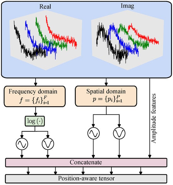
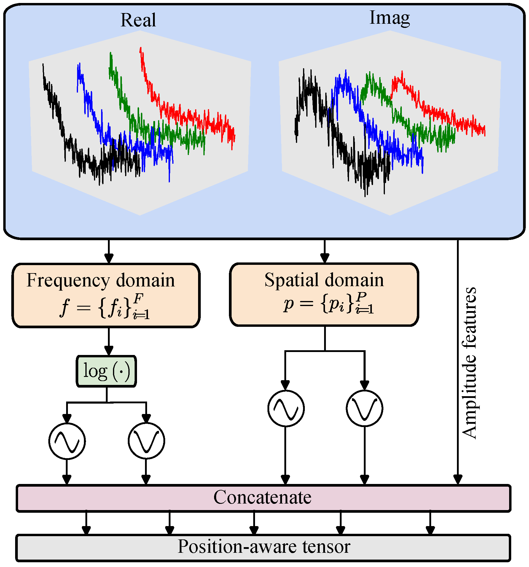
Inspired by the positional encoding method proposed by Vaswani et al. [32], we employ a sinusoidal positional encoder for both frequency and spatial coordinates. EMPE explicitly encodes FDEM data in frequency and space and combines this information with EM-response amplitudes to provide a physically informed, position-aware input to the subsequent model backbone. Because EMPE is defined analytically using sine and cosine functions without introducing additional trainable parameters, it offers stable behavior and good generalization when training data are limited. By selecting a wide range of scale factors appropriately, EMPE captures both slowly varying global trends and rapidly varying local structures along the frequency and spatial axes while interleaving sine and cosine components along the channel dimension. The structure of EMPE is shown in Figure 1.
Figure 1.
Structure of the frequency and spatial encoder.
The encoding is computed as in Equations (1)–(3). For each frequency , we map it to the logarithmic domain and normalize it to obtain a log-frequency variable . Using a set of predefined scale factors , we compute multi-scale sine components (even k) and cosine components (odd k). Similarly, with another set of scale factors , we compute the spatial sine and cosine encodings. In implementation, our encoder produces a tensor with these components interleaved along the channel dimension so that each consecutive set of channels encodes the complete pattern for the corresponding frequency and sampling position. In the network architecture, is combined with the hidden feature embedding of the EM signals.
2.2. Diffusion Model
Denoising diffusion probabilistic models (DDPMs) provide an important theoretical background for diffusion-based generative modeling [33]. In the conventional DDPM formulation, data are gradually perturbed by a predefined stochastic noising process and are then recovered through a learned reverse denoising chain. In the continuous-time setting, diffusion-based generation can be described by an Itô stochastic differential equation (SDE). Song et al. [34] further showed that the SDE admits an equivalent deterministic probability-flow formulation with the same time-dependent marginal distributions. Motivated by this deterministic flow viewpoint, EMDiC is implemented using conditional flow matching (CFM) rather than a discrete DDPM with a predefined noise schedule [35,36]. Specifically, a continuous transport path is constructed between a Gaussian source distribution and the clean secondary-field FDEM signal distribution. Let denote the clean secondary-field FDEM signal, let denote the Gaussian source variable, let denote the intermediate state on the prescribed path, and let denote the observation condition extracted from the noisy measurement together with the auxiliary physical descriptors. The prescribed forward path is defined as
Here, corresponds to the Gaussian source distribution and corresponds to the target clean-signal distribution. Thus, the denoising task is reformulated as learning a conditional continuous flow that transports samples from the Gaussian source to the clean-signal manifold under the guidance of the noisy observation. To parameterize the conditional generation process, the network is implemented in the x-prediction form. It directly predicts the clean endpoint on the prescribed path rather than an auxiliary noise term. The predictor is defined as
where denotes the network prediction of the clean signal conditioned on the intermediate state , the time variable t, and the observation condition . For the prescribed path in Equation (4), direct differentiation gives
Replacing the unknown clean endpoint
by its network estimate gives the learned conditional velocity field
where denotes the deterministic flow field that transports the current state toward the clean-signal distribution. During inference, the generation process starts from the Gaussian source and integrates the learned conditional flow from to . In this work, uniform-step forward Euler integration is adopted with . Let the interval be divided into uniform steps and define
The reverse denoising process is implemented by discretizing the learned conditional flow field with Euler updates. The numerical update then follows
Equation (9) shows that each integration step moves the current state toward the predicted clean endpoint by a controlled fraction, and the final denoised estimate is obtained as .
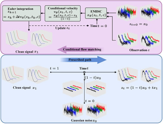
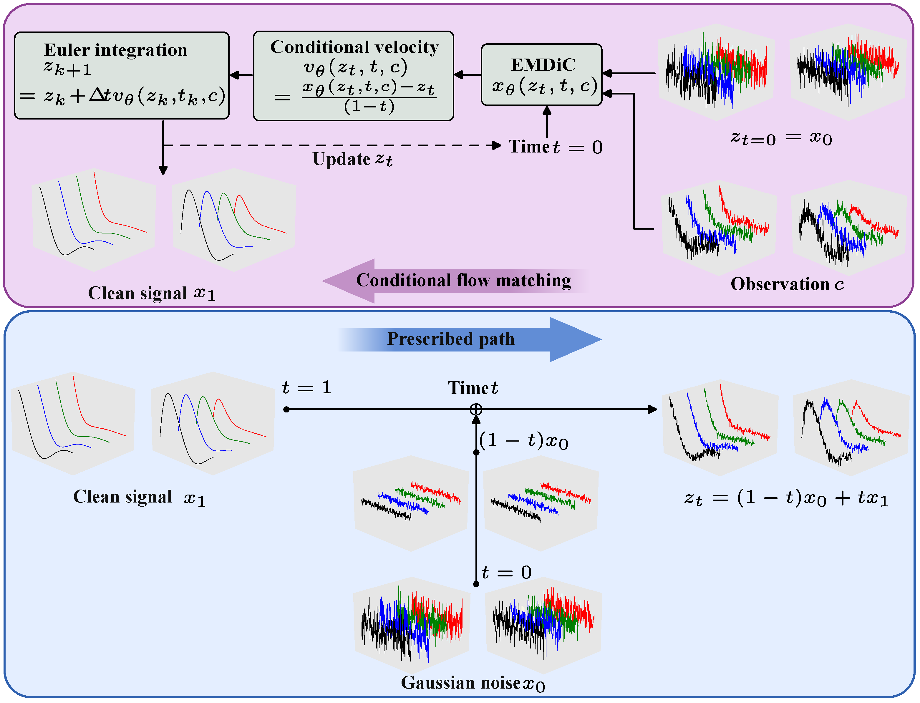
The complete conditional generation process of EMDiC is shown in Figure 2. Given the noisy observation and the time variable as conditions, the model predicts the clean endpoint on the prescribed path, constructs the corresponding conditional velocity field, and transports the state from Gaussian noise to the clean signal by Euler integration. The predictor in Equation (5) is implemented by EMDiC. To ensure high throughput and scalability for multi-frequency FDEM signal denoising, EMDiC adopts convolutional blocks and a U-Net-style hourglass backbone, which together provide efficient conditional feature extraction and multiscale information fusion.
Figure 2.
Overall conditional flow matching framework of EMDiC.
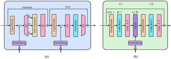
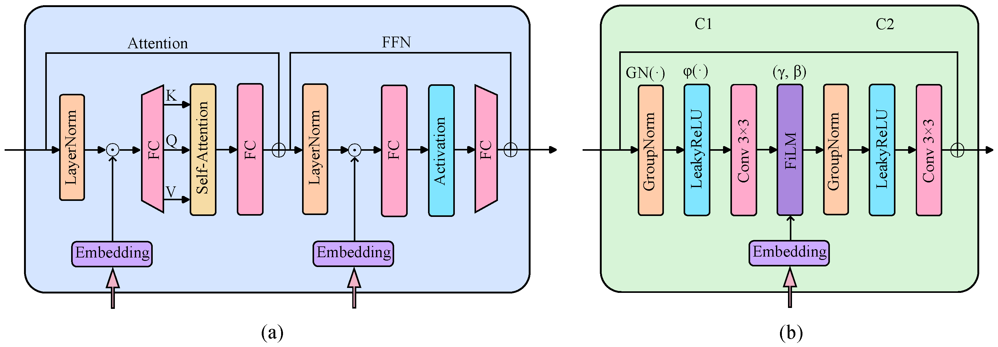
We use convolutional (Conv) blocks in EMDiC rather than the Transformer blocks used in Vision Transformer (ViT) because self-attention increases inference cost and latency. The two block types are compared in Figure 3. The Conv block removes self-attention, replaces the FC layers with convolutions, and uses two consecutive convolution layers with feature-wise linear modulation (FiLM) applied between them, as defined in Equation (10), where the feature-wise affine parameters are . Before each convolution, the input is normalized with GroupNorm () and passed through a LeakyReLU activation (). The block also uses a residual connection that adds the input directly to the output.
where ⊙ denotes element-wise multiplication with broadcasting over spatial dimensions.
Figure 3.
Comparison between the Transformer block and the Conv block: (a) Transformer block; (b) basic Conv block.
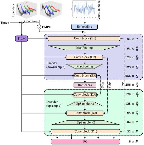
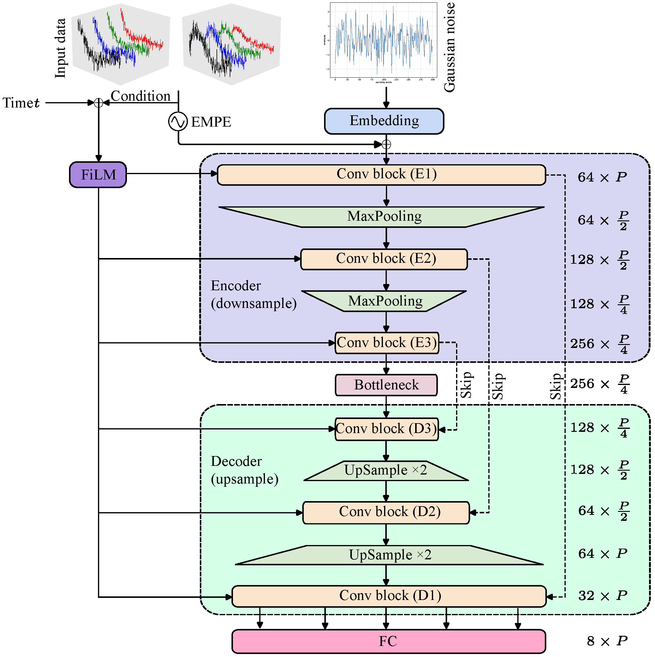
The overall network uses a U-Net hourglass architecture. The encoder progressively downsamples the feature resolution, and the decoder upsamples it back to the original scale. Each encoder module is linked to the corresponding decoder module through a skip connection. The architecture is shown in Figure 4. Because Conv blocks with a kernel have a limited receptive field, we use max pooling in the encoder to reduce spatial resolution and enlarge the effective receptive field. The decoder restores high-resolution structure, while the skip connections preserve local details and support global consistency. The noisy signal and time variable t are embedded as conditions and injected into the backbone through a dedicated conditioning branch. This branch extracts features from the observed signal and maps them to the FiLM parameters, allowing the intermediate feature maps to be modulated under the observation condition . This conditioning improves the controllability and fidelity of the reconstructed output.
Figure 4.
Overall architecture of the EMDiC hourglass network.
2.3. Composite Loss
Using an x-loss based on direct prediction can lead to highly imbalanced gradient contributions between high-noise and low-noise time steps, which can harm training stability. The v-loss reweights errors across time steps and yields more stable behavior. We therefore use the v-loss as the primary term and combine it with a physics-informed weighted composite loss. The overall loss is computed as follows:
- First-order total variation (TV): Equation (13) penalizes absolute first differences to suppress ringing and high-frequency spikes, yielding piecewise smoothness with edge preservation.
- Peak saliency constraint: Equation (14) matches the ratio between the baseline and the peak in prediction and ground truth, encouraging a dominant main peak with low background energy.
- Cosine similarity: Equation (15) emphasizes waveform shape alignment rather than amplitude magnitude, providing useful gradients even when scale differs.
- Soft full width at half maximum (FWHM): Equation (16) matches pulse width using a differentiable sigmoid-based half-peak indicator, approximating the number of samples above half peak.
- Masked second-difference curvature: Equation (17) penalizes sharp bends inside the pulse using a soft half-peak mask, controls mask hardness, and smaller approaches a hard threshold.
3. Model Training
3.1. Production of Sample Dataset
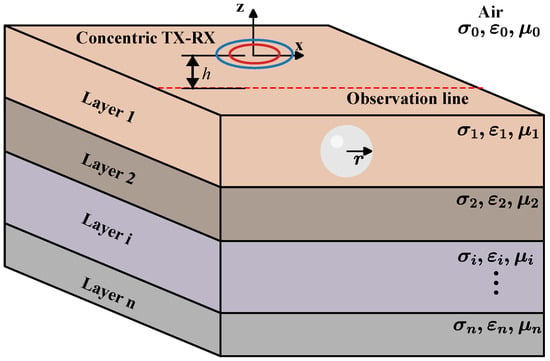
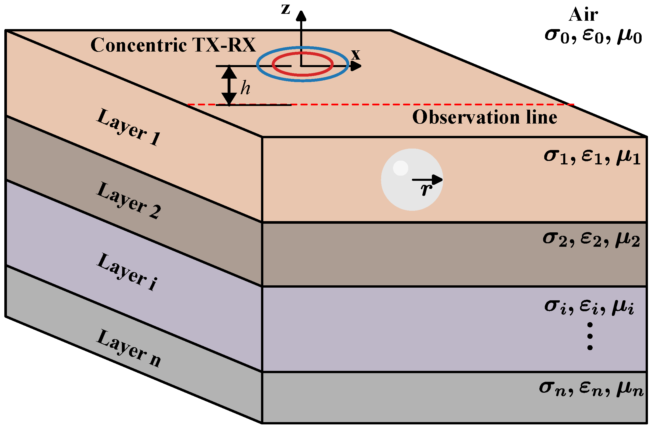
A training dataset with sufficient diversity and reliable ground-truth labels is essential for denoising. To simulate EM signals measured by practical instruments and improve robustness to noise, we construct the dataset through numerical simulation rather than field acquisition. Clean data are generated by forward modeling the EM responses of subsurface anomalies in a layered conductive earth model with a concentric TX–RX coil configuration and a 3D magnetic dipole target [37,38]. Figure 5 shows the adopted layered-earth model with the 3D magnetic dipole target. The forward model incorporates target properties such as conductivity, permeability, and geometry to compute multi-frequency magnetic-field responses, which allows clean signals to be generated under controlled geological settings.
Figure 5.
3D magnetic dipole target in a layered-earth model.
To match typical GEM-3 measurement conditions, the scan region of the concentric TX–RX coils was restricted to along the observation line. The TX coil operated at four excitation frequencies: 125.0, 1225.0, 2925.0, and 5925.0 Hz. The sampling length along the observation line was fixed at P = 200 points. The physical settings are summarized in Table 1. By combining different model parameters, we generated clean samples with diverse amplitudes and waveform shapes for both a uniform half-space model and a two-layer model. For each sample, the real and imaginary responses at the four operating frequencies were stacked along the channel dimension. Each clean or noisy sample was organized as an input tensor , where is the number of channels and P = 200 is the number of sampling points along the observation line.
Table 1.
Parameter settings of the layered-earth and target models.
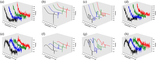
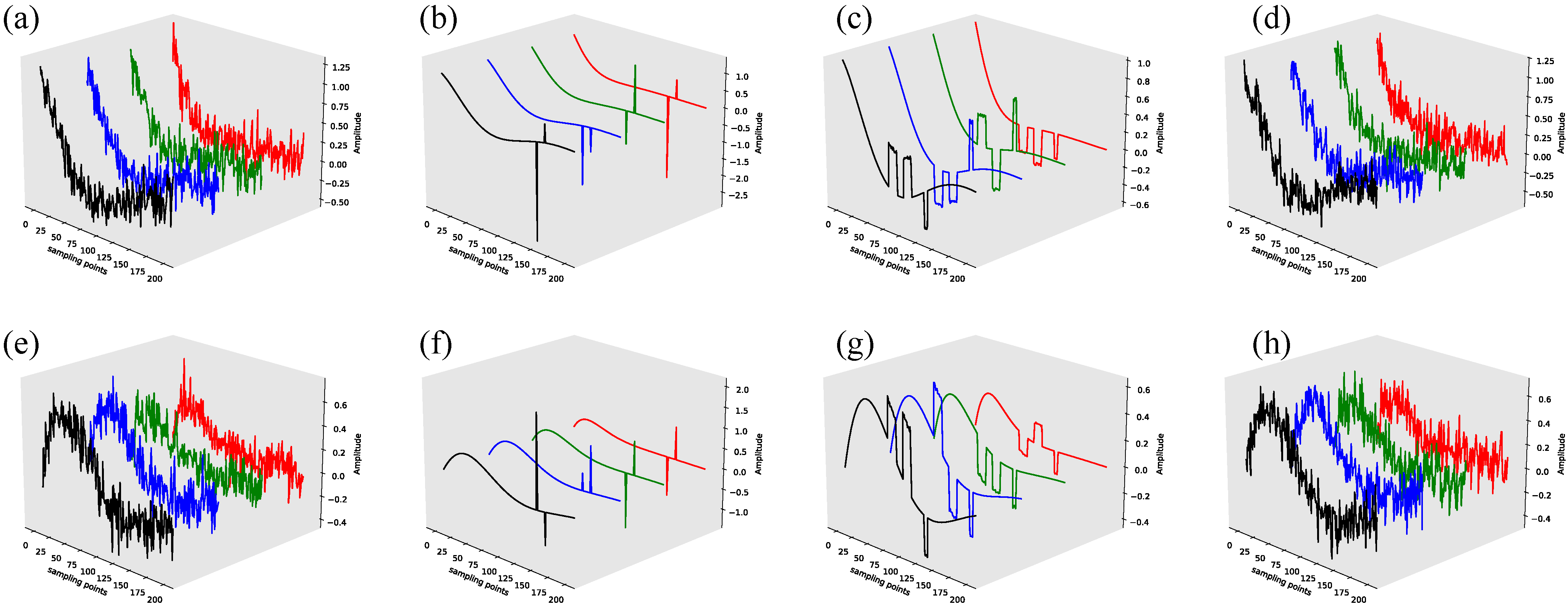
To simulate the mixed interference encountered in practice, we add random pulse noise, random square-wave noise, and additive white Gaussian noise (AWGN). The AWGN level was set within . These noise components were added to the clean EM signals to build the noisy dataset. Representative noise waveforms are shown in Figure 6. Among them, AWGN usually has the largest effect on the effective Signal-to-Noise Ratio (SNR). For pulse noise, the real and imaginary parts share the same pulse positions but have different amplitudes, which can introduce oscillatory artifacts during denoising. For random square-wave noise, the real and imaginary parts are generated at the same positions but also with different amplitudes. The longer oscillation duration of this noise makes signal–noise separation more difficult.
Figure 6.
Typical noise waveforms: (a–d) real part of different types of noise and (e–h) imaginary part of different types of noise. (a,e) AWGN, (b,f) random pulse noise, (c,g) random square-wave noise, and (d,h) combinations of different noise types.
In total, 150 k samples were acquired, including 108 k samples for the training set (), 12 k samples for the validation set (), and 30 k samples for the test set (). Because the variability among targets and layered configurations induces fluctuations in the EM signal, all samples were normalized prior to network training to mitigate bias and numerical instability. A Z-score normalization was applied along the sampling point dimension because it preserves the structural characteristics of the samples, including the positive–negative sign polarity. This normalization enforces zero-mean and unit-variance statistics for each sample channel while preserving waveform morphology, thereby improving optimization stability and cross-sample generalization. Let denote one sample, where P is the number of sampling points and C is the number of feature channels. The normalized value at the i-th sampling point is defined as
where is a small positive constant. The mean and standard deviation are computed within the same sample over the sampling points:
3.2. Model Setting and Training
The training samples were randomly shuffled before training. To evaluate the proposed model, EMDiC was compared with 1D U-Net, four diffusion-based variants, and four additional baselines. The diffusion-based variants are Diffusion model with RMSE (DM w/RMSE), Diffusion model without EMPE (DM w/o EMPE), Diffusion model without FiLM (DM w/o FiLM), and the basic Diffusion model (DM). The other baselines are BP [39], DnCNN [40], GRU [41], and ResNet [42]. An ablation study was also designed to assess the contribution of each term in the composite loss, as described in Section 4.
All baselines and comparison variants were trained under the same basic hyperparameter setting, as summarized in Table 2. After tuning, the final setting used 200 epochs, a batch size of 64, and a learning rate of . EMDiC, DM w/o EMPE, and DM w/o FiLM were optimized with the composite loss, while 1D U-Net, DM w/RMSE, DM, BP, DnCNN, GRU, and ResNet were optimized with RMSE.
Table 2.
Training hyperparameters and optimization settings.
Early stopping was not used so that the full training trajectories of all models could be reported and compared directly. After each epoch, the current model was evaluated on the validation set, and the checkpoint with the lowest validation loss was selected for final testing. For models trained with RMSE, checkpoint selection was based on validation RMSE. For models trained with the composite loss, the corresponding validation composite loss was used.
The number of model parameters and the average training time per epoch are listed in Table 3. EMDiC has a parameter count comparable to the diffusion-based variants and remains much smaller than BP, which has the largest parameter count among all models. ResNet has the lightest architecture, while 1D U-Net, DnCNN, and GRU fall in the middle range. EMDiC has the longest average training time per epoch. Most of this cost comes from the multi-scale diffusion backbone, the iterative denoising process, and the additional computation required by the composite loss. The non-diffusion baselines are much faster, while the diffusion-based variants remain in a similar high-cost range. In short, EMDiC achieves better denoising with a moderate parameter count, but it requires longer training.
Table 3.
Model parameter number and runtime.
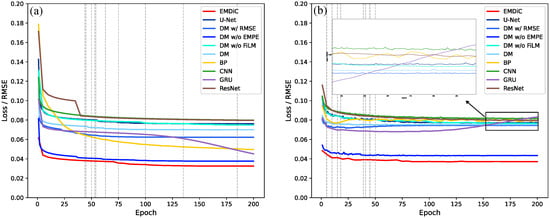
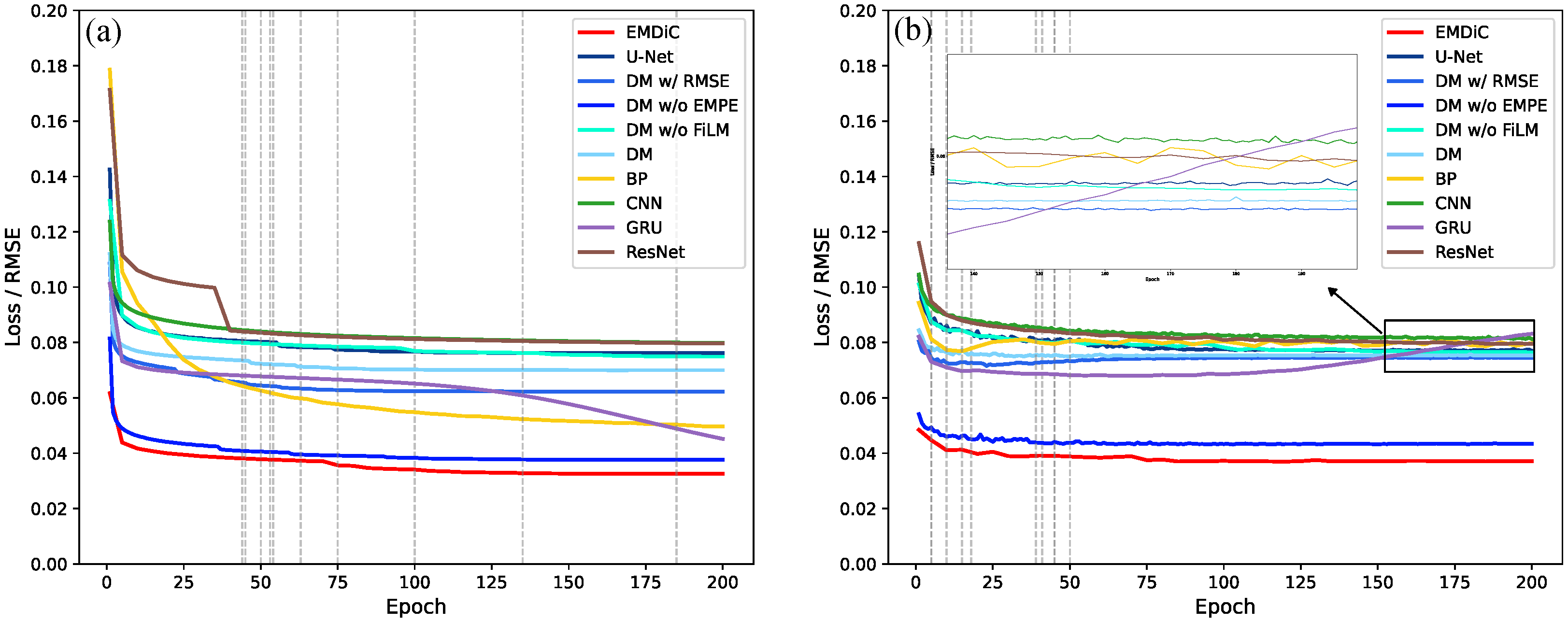
The training and validation loss curves are shown in Figure 7. Overall, the training loss decreases and converges as the number of epochs increases. In Figure 7a, EMDiC reaches the lowest training loss and finally converges to , indicating the strongest fitting ability among the compared models. DM w/o EMPE follows a similar trend but remains above EMDiC, while DM w/o FiLM stabilizes at a much higher training loss of , showing that removing FiLM weakens optimization even though the backbone is unchanged. Among the other baselines, 1D U-Net, BP, DnCNN, and ResNet all converge to visibly higher training losses than EMDiC. GRU reaches a lower training loss than those baselines, but it still remains inferior to EMDiC.
Figure 7.
Training and validation loss curves of EMDiC and the baseline models: (a) training loss curves; (b) validation loss curves.
The validation curves in Figure 7b show clear differences in generalization behavior. EMDiC maintains the lowest validation loss through most of training and finally stabilizes at . Its training–validation gap also remains small, which indicates stable convergence without obvious overfitting. DM w/o EMPE is the closest diffusion variant, with a higher validation loss of , suggesting that the composite loss contributes more than EMPE to generalization. DM w/RMSE and DM w/o FiLM both remain at higher validation losses, and DM w/o FiLM finally reaches , which shows that FiLM provides useful conditional guidance in the diffusion process. DM also stays clearly above EMDiC and DM w/o EMPE in the later stage, indicating that removing EMPE, FiLM, and the composite objective weakens generalization. Among the other baselines, 1D U-Net shows a relatively small gap but still lower final accuracy. BP drops markedly on the training curve but does not show the same improvement on the validation curve. DnCNN and ResNet also remain at relatively high validation losses, and GRU shows the clearest overfitting, because its training loss continues to fall while the validation curve becomes less stable in the later stage. Overall, these curves show that the diffusion framework, EMPE, FiLM, and the composite loss work together to give EMDiC the best generalization behavior.
3.3. Denoising Results on the Test Set
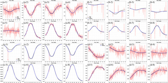
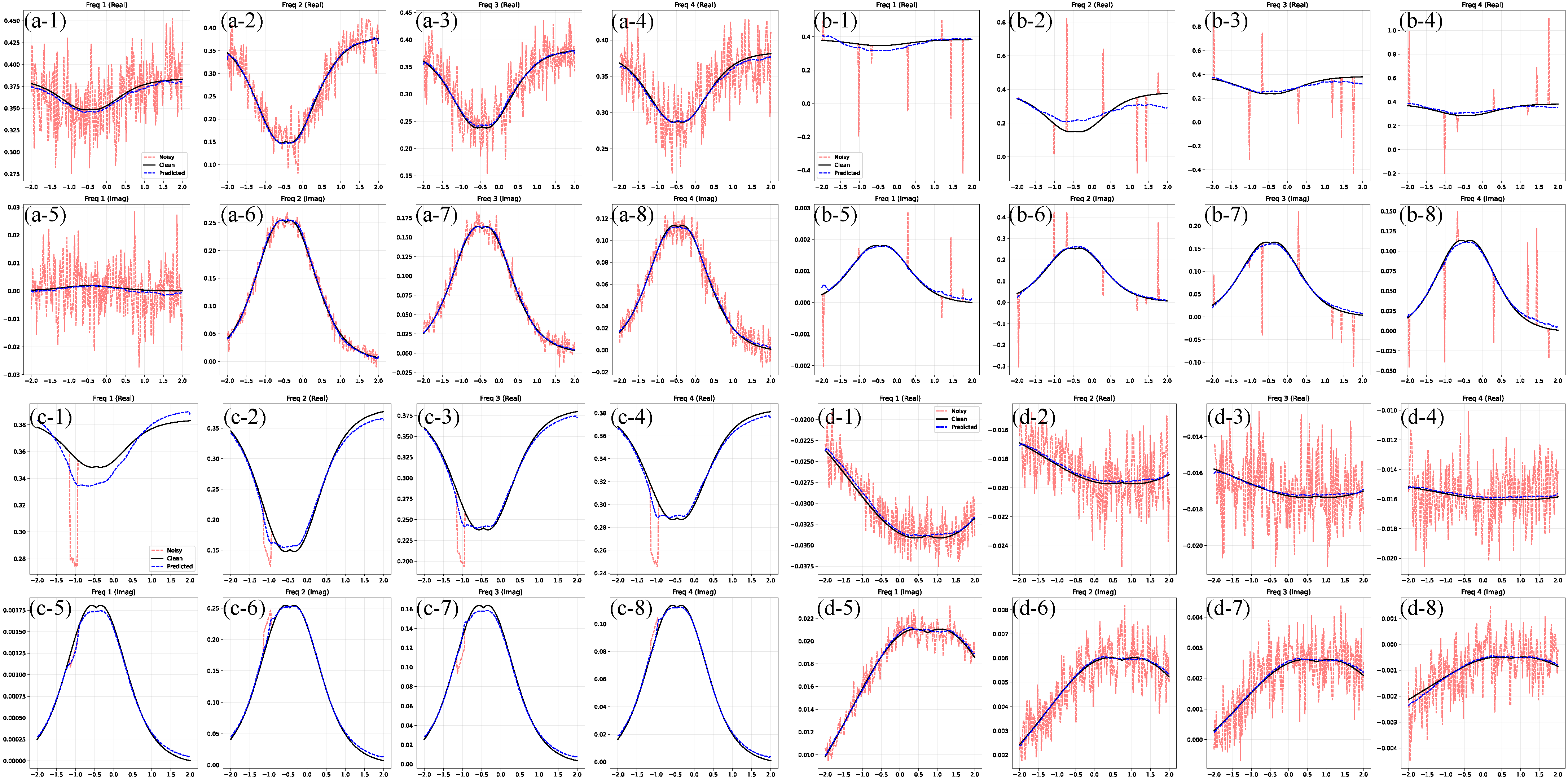
Representative denoising examples from the test set are shown in Figure 8. The red curves denote noise-contaminated signals, and the blue dashed curves show the outputs of the trained EMDiC model. These results indicate that EMDiC suppresses diverse interference patterns while preserving the main waveform morphology, including global trends and local extrema.
Figure 8.
Typical denoising samples from the testing set: (a) Gaussian noise, (b) pulse noise, (c) square-wave noise, and (d) mixed noise. For each case, subplots 1–4 show the real part and subplots 5–8 show the imaginary part.
In Figure 8a, the signal is mainly corrupted by Gaussian noise. The random noise distributed over the full trace is greatly reduced after denoising, and the reconstructed curve remains smooth and continuous. In Figure 8b, pulse noise introduces sparse impulsive spikes with large amplitudes. The model removes these outliers while preserving neighboring valid responses. Although slight deviations from the clean reference can be seen in Figure 8(b-1,b-2), the denoised curves preserve the overall waveform morphology and remain effective across the other frequency channels. In Figure 8c, square-wave noise causes step-like distortions and abrupt level changes. EMDiC restores baseline consistency and local transition profiles. Although denoising is less accurate at lower frequencies than at higher frequencies, EMDiC still recovers the signals well. Even for heavily corrupted cases such as Figure 8(c-1), it preserves waveform morphology. In Figure 8d, where multiple noise types coexist, the EMDiC output still follows the original signal pattern and suppresses most abnormal perturbations, indicating good robustness and generalization to unseen test samples.
4. Synthetic and Real Data Analysis
To demonstrate the effectiveness of EMDiC, this section first presents an ablation study on the composite loss, followed by quantitative comparisons on synthetic datasets with different noise levels and material categories, and finally analysis on experimentally acquired real data.
4.1. Ablation Study
To assess the contribution of each term in the physics-informed composite loss, we carried out an ablation study on the synthetic test set. The evaluation used test samples with an average input SNR of . All ablation settings were trained with the same hyperparameters described in Section 3. Performance was evaluated with RMSE, SNR, and normalized cross-correlation coefficient (NCC), where lower RMSE and higher SNR/NCC indicate better denoising. The loss weights were fixed as , and the shape-control parameter was fixed at . The results are summarized in Table 4. EMDiC performs best in all three metrics, which shows that the full composite loss gives the most balanced result in terms of pointwise accuracy, noise suppression, and waveform preservation. Compared with the rmse variant, the full objective reduces RMSE from to and also improves SNR and NCC. This result shows that RMSE alone is not sufficient to constrain denoising behavior.
Table 4.
Ablation study on the composite loss terms.
Among the leave-one-term-out variants, no_peak gives the smallest overall degradation when RMSE, SNR, and NCC are considered together, followed by no_width, while no_curv has an intermediate effect. The largest degradation is caused by removing the TV or cosine term. This pattern suggests that the TV and cosine terms are the most important in the present setting. The TV term helps the model learn smooth and stable denoising trajectories, which is especially important for diffusion-based reconstruction. The cosine term constrains global waveform agreement and adds shape-level supervision beyond pointwise fitting. When either term is removed, the balance among smoothness, shape consistency, and noise suppression becomes weaker. The relatively small influence of removing the peak term suggests that explicit peak supervision is less critical for the present dataset. One reason may be that the training set includes “none” cases, so the model does not rely mainly on peak-focused supervision to remain stable. The width term also has a limited effect. Since the training set is restricted to single shallow targets, response-width differences among samples remain limited, which reduces the contribution of the width constraint. The curvature term mainly acts as a local geometric regularizer. Removing it causes a moderate degradation, which suggests that it helps refine local waveform geometry but does not dominate the final denoising result.
The rmse variant is not the worst-performing configuration. This result suggests that the composite-loss terms are coupled during optimization rather than acting independently. Once one term is removed, the remaining terms may become less complementary and may no longer provide the same effect as in the full objective. Overall, the ablation study shows that the composite loss is effective because its terms provide complementary constraints during denoising. These observations support the use of the full composite loss in EMDiC as a robust and well-balanced objective for FDEM signal denoising.
4.2. Synthetic Data Analysis
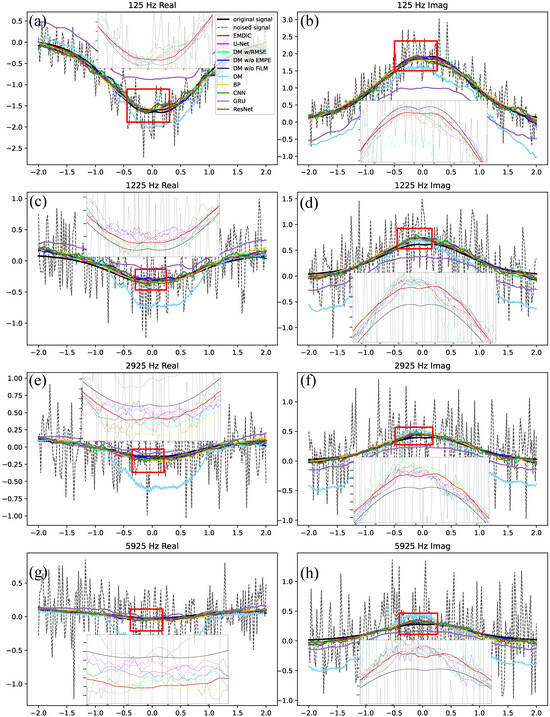
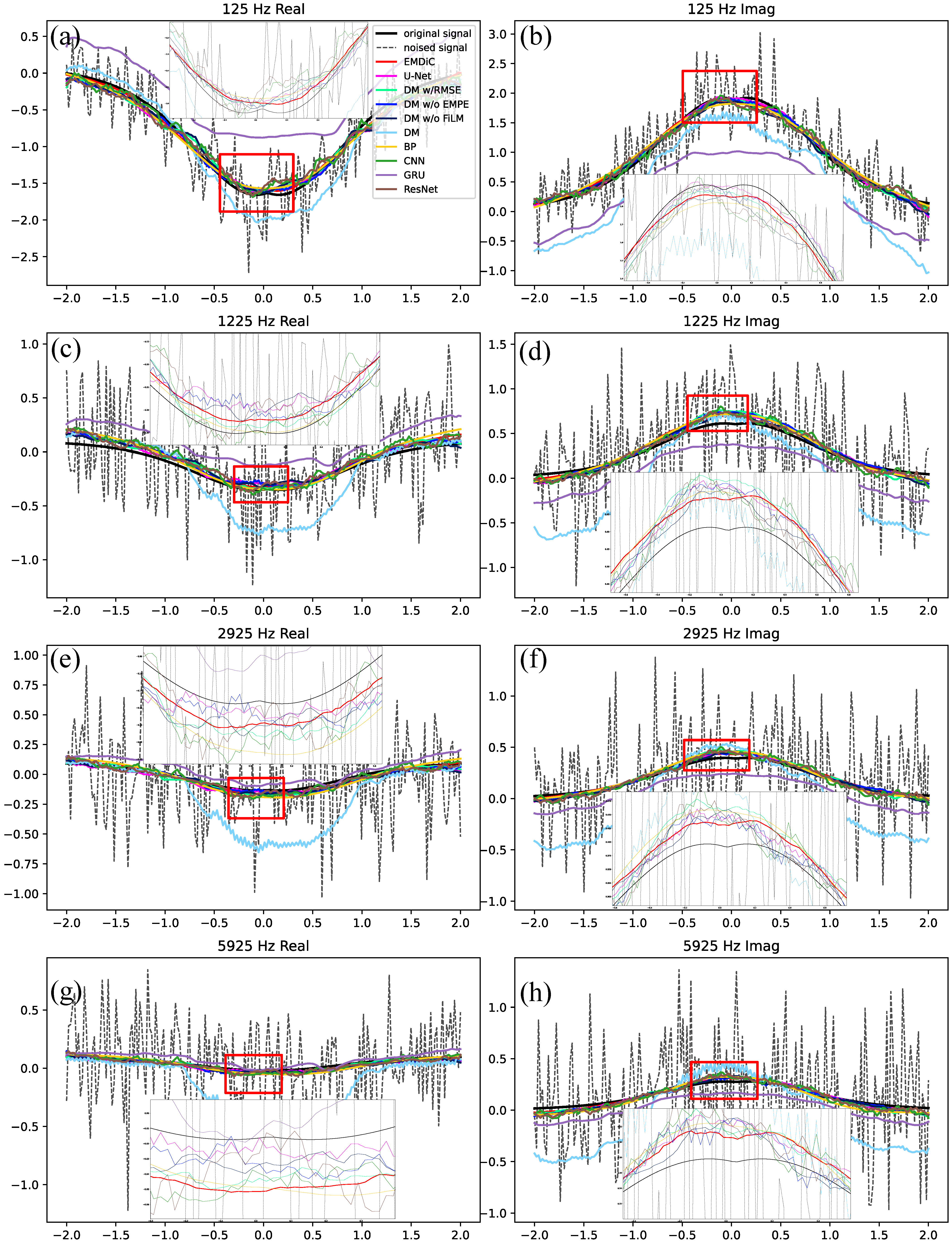
Figure 9 shows a representative comparison for one iron sample over four real and four imaginary channels at [125.0, 1225.0, 2925.0, 5925.0] Hz. Each panel contains the full denoising trace, and the red box marks the enlarged region. EMDiC gives the closest agreement with the clean response in both the real and imaginary channels. In the real channels, it recovers the trough shape and the recovery slope while maintaining stable behavior in the response region. In the imaginary channels, it preserves the response peak and the amplitude variation around the anomaly.
Figure 9.
Representative denoising comparison on an iron sample. (a) 125.0 Hz real, (b) 125.0 Hz imaginary, (c) 1225.0 Hz real, (d) 1225.0 Hz imaginary, (e) 2925.0 Hz real, (f) 2925.0 Hz imaginary, (g) 5925.0 Hz real, and (h) 5925.0 Hz imaginary.
Compared with EMDiC, 1D U-Net still captures the overall response envelope but tends to smooth local extrema and broaden the transition zones around the anomaly. Among the diffusion-based variants, DM w/o EMPE remains the closest to EMDiC. This indicates that the diffusion backbone and the composite loss can already learn the main waveform shape without EMPE. The remaining advantage of EMDiC appears mainly in cross-frequency consistency and the recovery of finer local details, which suggests that EMPE provides useful physical guidance for frequency-aware reconstruction. DM w/o FiLM also suppresses much of the interference, but it adapts less well to the local response region than EMDiC. DM w/RMSE remains below EMDiC and shows more visible mismatches around peaks, troughs, and tails. This is consistent with the ablation results, which showed that the RMSE-only objective is weaker at preserving waveform structure than the full composite loss. The plain DM deviates even more strongly in several channels. In some cases it performs worse than 1D U-Net, which shows that diffusion alone is not sufficient and that physical guidance is important for stable FDEM reconstruction.
For most models, the lower-frequency channels show larger local deviations than the higher-frequency channels. This suggests that the low-frequency response is more sensitive to residual interference and local smoothing errors. Even so, EMDiC remains the most balanced model in terms of noise suppression, local-detail preservation, and global continuity across the compared channels. Among the other baselines, BP, DnCNN, and ResNet generally recover the broad trend, but they still leave more residual oscillations or oversmoothing than EMDiC in the anomaly region. GRU shows the largest waveform distortion and baseline drift, so its reconstruction is the least consistent with the clean response. Overall, these results show that EMDiC provides a better balance between noise suppression and detail preservation for synthetic subsurface target responses.
To evaluate performance under different noise conditions, three noise levels are considered: high noise (∼ dB), medium noise (0∼5 dB), and weak noise (15∼20 dB). Table 5 summarizes the quantitative results in terms of RMSE, SNR, and NCC. EMDiC performs best in all three metrics at all three noise levels. Compared with 1D U-Net and the plain DM, the results also show that the gain does not come from diffusion alone. The improvement comes from physically guided diffusion-based reconstruction, especially under medium and high noise. The large gap between EMDiC and DM further shows that diffusion models need physical guidance and structured optimization to recover stable EM-response waveforms.
Table 5.
Quantitative comparison of different models under multiple noise levels.
Compared with 1D U-Net, EMDiC shows consistent gains at all three noise levels, and the advantage is especially clear under medium and high noise. Among the diffusion-based variants, DM w/o EMPE remains the strongest ablation, which indicates that the composite loss provides a large part of the denoising benefit, while EMPE adds complementary physical guidance. DM w/RMSE performs noticeably worse than EMDiC and generally remains below DM w/o EMPE. This agrees with the ablation results, which showed that replacing the composite loss with RMSE weakens waveform preservation. DM w/o FiLM also remains below EMDiC at all three noise levels. The gap becomes smaller under weak noise, but its lower SNR and NCC still indicate weaker conditional adaptation once FiLM is removed. Among the other baselines, BP, DnCNN, and ResNet remain below EMDiC at all noise levels, while GRU degrades much more severely under medium and high noise.
To examine denoising behavior for different target categories, four material types are considered: iron, aluminum, cavity, and none. The quantitative results are summarized in Table 6. EMDiC performs best for iron, aluminum, and cavity, while remaining competitive but not dominant for none. This pattern suggests that the proposed framework is most useful when the target response contains clear EM-induced structure. Its advantage becomes smaller when the sample contains little effective physical-response information.
Table 6.
Quantitative comparison of different models under multiple material types.
For iron and aluminum, EMDiC outperforms 1D U-Net and the diffusion-based variants. The advantage is especially clear for iron, where EMDiC shows a clear margin over all other models in RMSE, SNR, and NCC. This indicates that when the target response is strong, the combination of diffusion modeling, EMPE guidance, FiLM, and the composite loss is most effective. For aluminum, the gaps become smaller but remain consistent, which shows that EMDiC is not only effective for strong inductive targets but also stable for weaker metallic responses. Across these two materials, DM w/o EMPE is the strongest diffusion ablation. This suggests that the composite loss contributes substantially to target-response reconstruction, while the remaining gain of EMDiC over DM w/o EMPE confirms that EMPE provides useful complementary guidance. DM w/o FiLM also remains below EMDiC for both iron and aluminum, which suggests that FiLM helps the model adapt to different target-response patterns. For cavity and none, the differences among the leading models become much smaller. In the cavity case, EMDiC still gives the best overall result, although the margin is much narrower than for iron and aluminum. In the none case, EMDiC no longer performs best. This is reasonable because the none category contains little effective physical-response information, so the physics-guided constraints used by EMDiC become less informative and can slightly limit performance. In that setting, denoising is closer to background smoothing, and non-physics-guided networks such as ResNet can perform slightly better.
4.3. Real Data Analysis
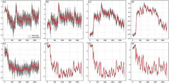
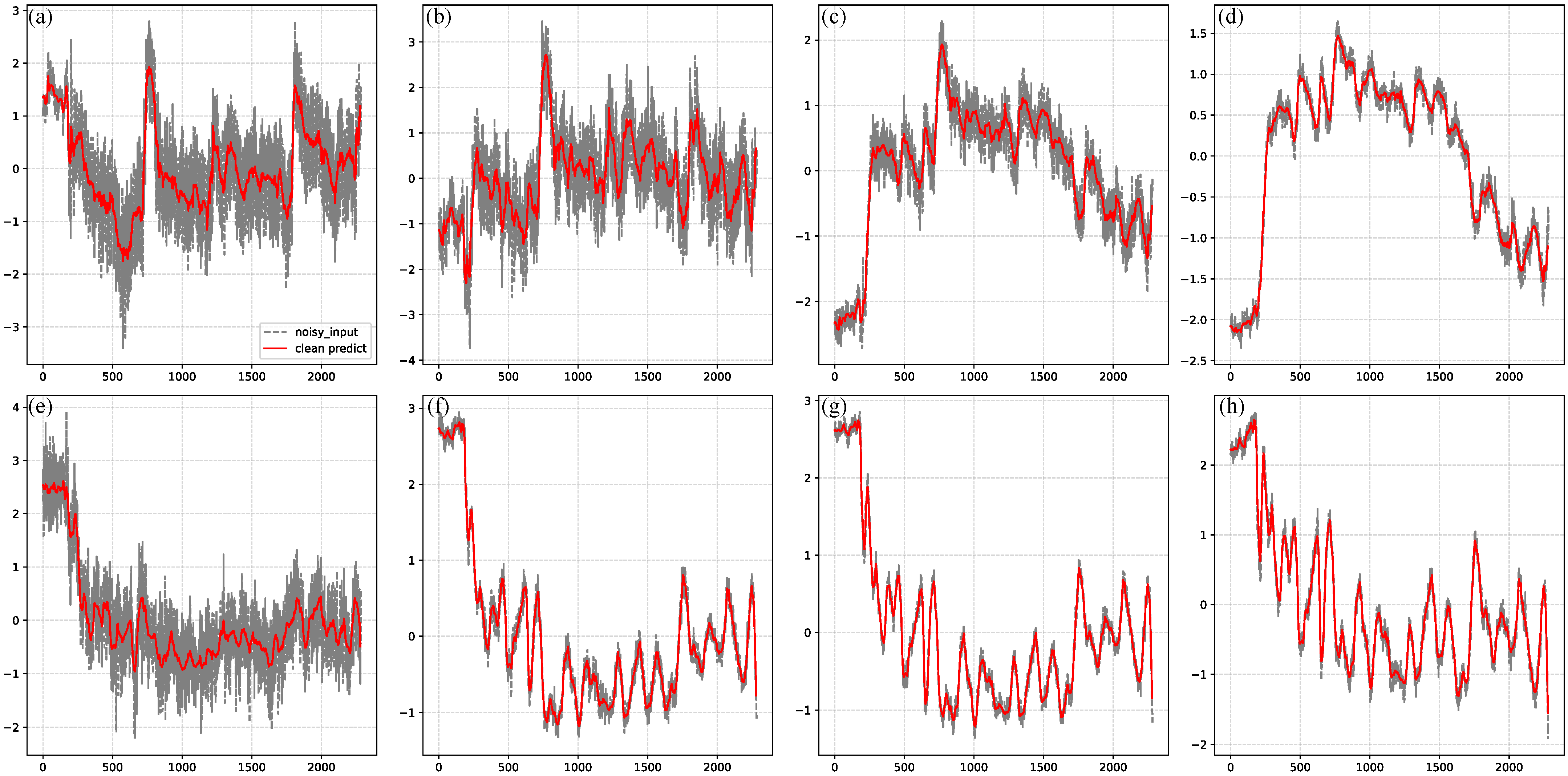
To assess the practical performance of EMDiC, we applied it to field data collected in Zhejiang Province, China, with our laboratory’s self-developed GEM-3 system [38]. In field surveys, the data often contain responses from multiple targets and form long sequences, whereas EMDiC is trained on short single-target samples. To account for target-absent segments that frequently appear in long sequences, a “none” option was included during training to reduce neural-network hallucinations during inference. A sliding-window strategy was therefore used for long-sequence data. The sequence was processed with a shifted window along the sampling axis, each window was denoised by EMDiC, and the outputs were then merged back into the full sequence. The field-data sequences analyzed in this subsection were processed using the same Z-score normalization described in Section 3. The GEM-3 sampling rate is about , or about 10 sample points per second, and the along-track horizontal resolution is about . The window length and shift step were set to 50 and 5 sample points to obtain smoother transitions. Figure 10 compares the original field data with the EMDiC output for both real and imaginary components. The denoised curves suppress oscillations while preserving the main peaks, troughs, and boundaries, which indicates good generalization from short synthetic samples to long field measurements.
Figure 10.
Field-data denoising results of EMDiC with window-based inference. Panels (a–d) show the real part and panels (e–h) show the imaginary part. Panels (a–e) correspond to 125.0 Hz, panels (b–f) to 1225.0 Hz, panels (c,g) to 2925.0 Hz, and panels (d–h) to 5925.0 Hz.
To quantitatively evaluate the denoising performance on field data, three proxy metrics, the peak-position drift (PPD), the main-lobe width variation (MWV), and the inter-frequency coherence (IFC), were introduced. Let and denote the normalized original and denoised 1D signals at the m-th operating frequency , where corresponds to the four frequencies and denotes the sampling index along the observation line.
PPD is used to quantify the positional deviation of response extrema after denoising. It is defined as
where and denote the positions of the k-th matched extremum pair in the original and denoised signals, denotes the number of matched response pairs at frequency , P denotes the signal length, and denotes the number of operating frequencies. A smaller PPD indicates better preservation of the response positions after denoising.
MWV is used to quantify the variation in response width after denoising. It is defined as
where and denote the half-amplitude support regions containing the k-th matched extremum in the original and denoised signals, denotes the number of sampling points in the support region, and is a small positive constant for numerical stability. A smaller MWV indicates better preservation of the response width after denoising.
Based on NCC, IFC is used to quantify the structural consistency across adjacent operating frequencies before and after denoising. It is defined as
where is the metric defined above, and and are the IFC values of the original and denoised signals. A higher IFC indicates stronger cross-frequency consistency of the response morphology.
As summarized in Table 7, EMDiC improves cross-frequency consistency after denoising while preserving the principal response geometry at an acceptable level. Specifically, the average IFC increases from 0.6969 for the original signals to 0.7834 for the denoised signals, indicating that the influence of noise on cross-frequency consistency is reduced and that the resulting frequency-dependent response pattern becomes more coherent overall. For the real component, the IFC increases from 0.6355 to 0.6692, whereas for the imaginary component it increases from 0.7583 to 0.8975. The larger improvement observed in the imaginary component indicates that EMDiC yields a greater enhancement of cross-frequency consistency for the imaginary responses, suggesting that the suppression of noise contamination is more effective in the imaginary part than in the real part. The average PPD is 0.2246, indicating that the matched response extrema remain within a limited positional deviation after denoising. The average MWV is 0.2222, indicating that the denoising process does not introduce severe distortion into the matched response widths.
Table 7.
Quantitative proxy metrics of field-data denoising performance.
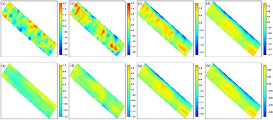
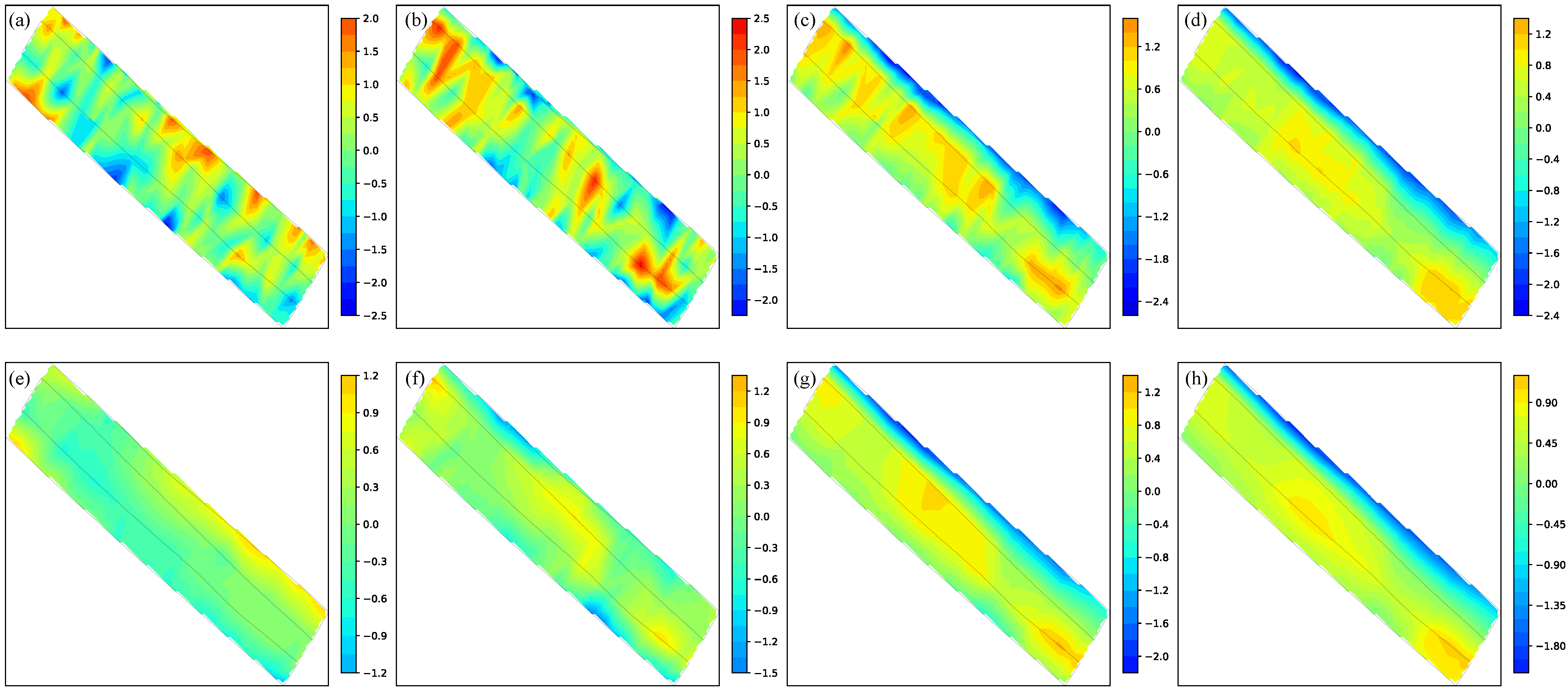
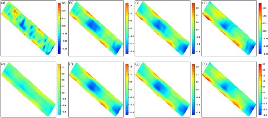
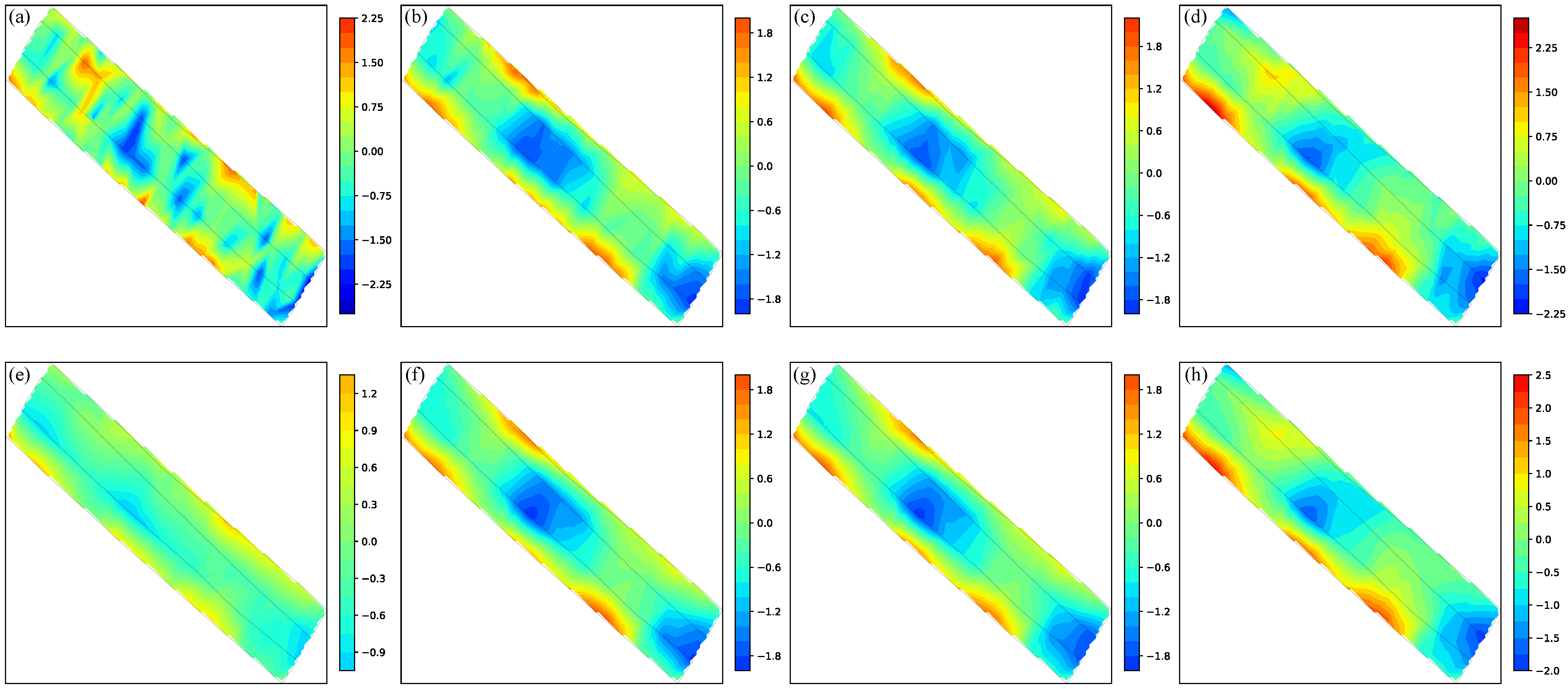
We also visualize the spatial distribution by interpolating the measurements into 2D maps. For each frequency and for each real or imaginary component, the normalized responses at the GPS sampling locations were mapped onto a regular Cartesian grid covering the survey area and then linearly interpolated with the built-in SciPy interpolation function. The same procedure was applied to both the original and denoised data. The discrete responses measured at GPS locations were converted into continuous 2D heatmaps on a grid. Figure 11 and Figure 12 were generated by spatially interpolating the 1D multi-frequency signals shown in Figure 10. Figure 11 shows the real part and Figure 12 shows the imaginary part. In each figure, the original maps in panels (a)–(d) contain background interference and local patches that partly obscure the main response region and weaken the continuity of the anomaly boundary. After denoising, the predicted maps in panels (e)–(h) become more spatially coherent, with smoother background variations and clearer anomaly-to-background contrast, so the dominant response region and its boundaries can be identified more reliably. This behavior is consistent with the quantitative results in Table 7. The lower IFC values of the original data indicate weaker structural coherence across frequencies, while the higher IFC values after denoising show that noise-induced spatial inconsistency is suppressed. The nonzero PPD values suggest that part of the denoising effect appears as a correction of noise-induced extremum displacement. The nonzero MWV values indicate that denoising also reshapes the effective width of the response by suppressing noise-induced broadening.
Figure 11.
2D heatmaps of the real-part field data before and after denoising by EMDiC. Panels (a–d) show the original measurements and panels (e–h) show the denoised predictions. Panels (a,e) correspond to 125.0 Hz, panels (b,f) to 1225.0 Hz, panels (c,g) to 2925.0 Hz, and panels (d,h) to 5925.0 Hz.
Figure 12.
2D heatmaps of the imaginary-part field data before and after denoising by EMDiC. Panels (a–d) show the original measurements and panels (e–h) show the denoised predictions. Panels (a,e) correspond to 125.0 Hz, panels (b,f) to 1225.0 Hz, panels (c,g) to 2925.0 Hz, and panels (d,h) to 5925.0 Hz.
For the real component in Figure 11, the denoised maps preserve the large-scale response trend while suppressing irregular local oscillations. In the pair (a) and (e), the background fluctuations are markedly reduced after denoising, but the anomaly response also becomes less clear, indicating that the improvement at low frequency is less effective than that observed in the higher-frequency cases. In the pair (b) and (f), the response position becomes more readily discernible after denoising, although the overall contrast remains moderate. In the pairs (c), (g) and (d), (h), the denoised maps reveal the response region much more clearly from the noisy background, with a more continuous response and a sharper transition between the anomaly and background zones. These observations explain why the real-part IFC remains lower than the imaginary-part IFC in Table 7. Although EMDiC improves the cross-frequency coherence of the real component, the real-part responses are spatially less concentrated and less visually prominent, so the consistency gain remains moderate. The finite PPD and MWV values are also consistent with the visual behavior of the real-part maps, where part of the denoising effect appears as the correction of noise-induced local displacement and support broadening of the response structure.
For the imaginary component in Figure 12, the denoised maps provide quadrature information for interpreting the target-induced response. In the pair (a) and (e), the main response position remains identifiable even at low frequency, and the denoised result suppresses surrounding fluctuations while retaining the main anomaly trend. In the pairs (b) + (f) and (c) + (g), an additional side response appears near the central anomaly in the original maps, but this feature is no longer apparent after denoising. This suggests that the side response is caused by noise rather than by a stable target-induced structure. In the pair (d) and (h), the denoised map further improves the spatial continuity of the main anomaly and gives a cleaner transition from the central response region to the surrounding background. Compared with the real part, the imaginary response is more concentrated and more visually distinct across the subfigure pairs, which agrees with the higher IFC values in Table 7. The relatively low PPD indicates that the main response locations remain well aligned after denoising, while the nonzero MWV indicates that the effective support width is adjusted as fluctuations are suppressed. Overall, these results suggest that EMDiC improves the imaginary component more strongly than the real component.
Overall, the 1D and 2D results show that EMDiC improves the interpretability of field measurements. The denoised outputs suppress interference and spatial artifacts while preserving the main response envelopes, transition boundaries, and frequency-dependent spatial structure. Together with the quantitative metrics in Table 7, these results show that EMDiC reduces noise-induced degradation of cross-frequency coherence and restores response structures that were partly masked or distorted in the original data, without introducing obvious spurious anomalies in the main response region.
5. Conclusions
We propose EMDiC, a diffusion-based denoising framework for multi-frequency, complex-valued FDEM signals. By formulating denoising as a conditional generation problem, EMDiC combines an analytic frequency–spatial encoder with FiLM-conditioned convolutional hourglass blocks, allowing the model to capture dependencies across frequency channels and sampling positions while preserving waveform morphology. In addition, a physics-informed composite objective built on velocity reweighting and waveform regularization encourages physically plausible reconstructions and stabilizes optimization under severe noise.
To support reproducible training and evaluation, we constructed a physics-driven synthetic dataset via layered-earth forward modeling with embedded targets of different materials and mixed the clean responses with representative noise processes, as well as their combinations. Comparisons with 1D U-Net, diffusion-based variants, and representative neural-network baselines show that EMDiC achieves the best overall performance across the synthetic benchmarks, with especially clear advantages under medium-to-strong noise and for targets with pronounced induction responses. For target-absent none cases, the advantage becomes smaller because the physical prior is less informative, although EMDiC remains competitive.
The variant and ablation experiments further show that the composite loss provides a large part of the denoising benefit, while EMPE and FiLM supply complementary physical and conditional guidance for preserving waveform structure and cross-frequency consistency. Finally, real-data experiments using GEM-3 measurements with a sliding-window inference strategy and proxy metrics show that EMDiC generalizes from short synthetic samples to long field sequences, improving cross-frequency coherence while preserving dominant response positions and widths. These results indicate that physics-informed diffusion models trained on synthetic data can remain practically effective for real-world FDEM denoising.
Author Contributions
Conceptualization, Z.D.; methodology, Z.D.; software, Z.D.; validation, Z.D.; formal analysis, Z.D.; investigation, Z.D., M.G.; resources, Z.D., M.G. and Z.Q.; data curation, Z.D. and Z.Q.; writing—original draft preparation, Z.D.; writing—review and editing, Z.D. and X.Z.; visualization, Z.D.; supervision, X.Z.; project administration, X.Z.; funding acquisition, X.Z. All authors have read and agreed to the published version of the manuscript.
Funding
This research was funded by the National Natural Science Foundation of China, grant number 61172017.
Data Availability Statement
Data are contained within the article.
Conflicts of Interest
Author Zhijie Qu was employed by the company Artificial Intelligence Institute China Electronics Technology Group Corporation Beijing. The remaining authors declare that the research was conducted in the absence of any commercial or financial relationships that could be construed as a potential conflict of interest.
References
- Karaoulis, M.; Ritsema, I.; Bremmer, C.; Kleine, M.D.; Essink, G.O.; Ahlrichs, E. Drone-borne electromagnetic (DR-EM) surveying in The Netherlands: Lab and field validation results. Remote Sens. 2022, 14, 5335. [Google Scholar] [CrossRef] [Scilit]
- Nabighian, M.N.; Corbett, J.D. (Eds.) Electromagnetic Methods in Applied Geophysics: Volume 2, Application, Parts A and B; Society of Exploration Geophysicists: Houston, TX, USA, 1991. [Google Scholar] [CrossRef] [Scilit]
- Grandis, H.; Sumintadireja, P. A brief review for the proper application of magnetotelluric (mt) and controlled-source audio-frequency magnetotelluric (csamt) in geothermal exploration. In Proceedings of the 12th Annual Indonesian Geothermal Association Meeting & Conference, Bandung, Indonesia, 6–8 November 2012. [Google Scholar]
- Xiaodong, Q.; Chen, W.; Guangyou, F.; Hejun, Y. Detecting anomaly targets using handheld frequency domain electromagnetic system. Sens. Actuators A Phys. 2017, 268, 155–163. [Google Scholar] [CrossRef] [Scilit]
- Deidda, G.P.; Himi, M.; Barone, I.; Cassiani, G.; Ponsati, A.C. Frequency-domain electromagnetic mapping of an abandoned waste disposal site: A case in sardinia (italy). Remote Sens. 2022, 14, 878. [Google Scholar] [CrossRef] [Scilit]
- Su, Y.; Ren, X.; Yin, C.; Wang, L.; Liu, Y.; Zhang, B.; Wang, L. Multiscale 3-D stochastic inversion of frequency-domain airborne electromagnetic data. Remote Sens. 2024, 16, 3070. [Google Scholar] [CrossRef] [Scilit]
- Rasmussen, S.; Nyboe, N.S.; Mai, S.; Juul Larsen, J. Extraction and use of noise models from transient electromagnetic data. Geophysics 2017, 83, E37–E46. [Google Scholar] [CrossRef] [Scilit]
- Li, G.; Gu, X.; Chen, C.; Zhou, C.; Xiao, D.; Wan, W.; Cai, H. Low-frequency magnetotelluric data denoising using improved denoising convolutional neural network and gated recurrent unit. IEEE Trans. Geosci. Remote Sens. 2024, 62, 5909216. [Google Scholar] [CrossRef] [Scilit]
- Qu, X.X.; Li, T.L.; Wang, F. A study on the effect of bird’s attitude on helicopter EM data and the correction method. Chin. J. Geophys. 2014, 57, 1310–1321. (In Chinese) [Google Scholar] [CrossRef]
- Das, M.; Dey, A.; Sadhu, S.; Ghoshal, T.K. Adaptive unscented kalman filter at the presence of non-additive measurement noise. In Proceedings of the 2015 12th International Conference on Informatics in Control, Automation and Robotics (ICINCO), Colmar, France, 21-23 July 2015; IEEE: New York, NY, USA, 2015; Volume 1, pp. 614–620. [Google Scholar]
- Mallat, S.; Hwang, W. Singularity detection and processing with wavelets. IEEE Trans. Inf. Theory 1992, 38, 617–643. [Google Scholar] [CrossRef] [Scilit]
- Huang, N.E.; Shen, Z.; Long, S.R.; Wu, M.C.; Shih, H.H.; Zheng, Q.; Yen, N.C.; Tung, C.C.; Liu, H.H. The empirical mode decomposition and the hilbert spectrum for nonlinear and non-stationary time series analysis. Proc. R. Soc. Lond. Ser. A Math. Phys. Eng. Sci. 1998, 454, 903–995. [Google Scholar] [CrossRef] [Scilit]
- Ren, M.; Zhang, E.; Kang, Q.; Chen, L.; Zhang, M.; Gao, L. Adaptive SVD denoising in time domain and frequency domain. Appl. Sci. 2025, 15, 2034. [Google Scholar] [CrossRef] [Scilit]
- Yanju, J.; Li, D.; Yu, M.; Wang, Y.; Wu, Q.; Lin, J. A de-noising algorithm based on wavelet threshold-exponential adaptive window width-fitting for ground electrical source airborne transient electromagnetic signal. J. Appl. Geophys. 2016, 128, 1–7. [Google Scholar] [CrossRef] [Scilit]
- Ji, Y.; Li, D.; Yuan, G.; Lin, J.; Du, S.; Xie, L.; Wang, Y. Noise reduction of time domain electromagnetic data: Application of a combined wavelet denoising method. Radio Sci. 2016, 51, 680–689. [Google Scholar] [CrossRef] [Scilit]
- Liu, F.; Geng, Z.; Zhang, Q. The application of the EEMD method to the suppression of the motion induced noise in the grounded wire source airborne transient electromagnetic system. Geophys. Geochem. Explor. 2017, 41, 123–128. (In Chinese) [Google Scholar]
- Guo, Z.; Gong, X.; Han, J.; Liu, L.; Wu, Y.; Meng, F.; Kang, J. Research on a multiscale denoising method for low signal-to-noise magnetotelluric signal. IEEE Trans. Geosci. Remote Sens. 2022, 60, 5925018. [Google Scholar] [CrossRef] [Scilit]
- Xing, K.; Li, S.; Qu, Z.; Zhang, X. Time-domain electromagnetic noise suppression using multivariate variational mode decomposition. Remote Sens. 2024, 16, 806. [Google Scholar] [CrossRef] [Scilit]
- Feng, G.; Wei, H.; Qi, T.; Pei, X.; Wang, H. A transient electromagnetic signal denoising method based on an improved variational mode decomposition algorithm. Measurement 2021, 184, 109815. [Google Scholar] [CrossRef] [Scilit]
- Elouaham, S.; Nassiri, B.; El Abbadi, R.; El Melhaoui, O.; Said, S.; El Khadiri, K.; Dliou, A.; Latif, R.; Dlimi, S.; Zougagh, H. Hybridization Denoising Method for EMG Signals Using EWT and EMD Techniques. Int. J. Eng. Appl. (IREA) 2025, 13, 574–581. [Google Scholar] [CrossRef] [Scilit]
- Chen, K.; Pu, X.; Ren, Y.; Qiu, H.; Lin, F.; Zhang, S. TEMDnet: A novel deep denoising network for transient electromagnetic signal with signal-to-image transformation. IEEE Trans. Geosci. Remote Sens. 2022, 60, 5900318. [Google Scholar] [CrossRef] [Scilit]
- Sun, Y.; Huang, S.; Zhang, Y.; Lin, J. Denoising of transient electromagnetic data based on the minimum noise fraction-deep neural network. IEEE Geosci. Remote Sens. Lett. 2022, 19, 8028405. [Google Scholar] [CrossRef] [Scilit]
- Xu, B.; An, Z.; Han, Y.; Ye, G. Denoising CSAMT Signals in the Time Domain Based on Long Short-Term Memory. J. Geophys. Eng. 2024, 21, 507–516. [Google Scholar] [CrossRef] [Scilit]
- Liu, Z.; Zhang, X.; Li, D.; Liu, S.; Cao, K. Noise Elimination for Wide Field Electromagnetic Data via Improved Dung Beetle Optimized Gated Recurrent Unit. Geosciences 2025, 15, 8. [Google Scholar] [CrossRef] [Scilit]
- Xiao, G.z.; Li, G.; Zhang, K.; Wang, X.; Li, J. Controlled-Source Electromagnetic Data Denoising Based on Improved Vision Transformer. Appl. Geophys. 2025, 22, 1058–1077. [Google Scholar] [CrossRef] [Scilit]
- Gui, T.; Deng, J.; Li, G.; Chen, H.; Yu, H.; Feng, M. De-noising Magnetotelluric Data Based on Machine Learning. J. Appl. Geophys. 2024, 230, 105538. [Google Scholar] [CrossRef] [Scilit]
- Li, J.; Cheng, H.; Wang, J.; Zhang, X.; Tang, J. Coordinate Attention-Temporal Convolutional Network for Magnetotelluric Data Processing. IEEE Trans. Geosci. Remote Sens. 2024, 62, 5919114. [Google Scholar] [CrossRef] [Scilit]
- Wang, J.; Li, J.; Zhou, H.; Zhao, X.; Tang, J. MFF-DenseNet: Densely Connected Convolutional Network with Multi-Scale Feature Fusion for Magnetotelluric Noise Suppression. J. Geophys. Res. Solid Earth 2024, 129, e2024JB028869. [Google Scholar] [CrossRef] [Scilit]
- Peng, Z.; Yang, B.; Liu, L.; Xu, Y. Rapid Surrogate Modeling of Magnetotelluric in the Frequency Domain Using Physics-Driven Deep Neural Networks. Comput. Geosci. 2023, 176, 105360. [Google Scholar] [CrossRef] [Scilit]
- Trappolini, D.; Laurenti, L.; Poggiali, G.; Tinti, E.; Galasso, F.; Michelini, A.; Marone, C. Cold Diffusion Model for Seismic Denoising. J. Geophys. Res. Mach. Learn. Comput. 2024, 1, e2024JH000179. [Google Scholar] [CrossRef] [Scilit]
- Meng, C.; Gao, J.; Wu, B.; Chen, H.; Tian, Y. Posterior Sampling for Random Noise Attenuation via Score-Based Generative Models. Geophysics 2025, 90, V73–V85. [Google Scholar] [CrossRef] [Scilit]
- Vaswani, A.; Shazeer, N.; Parmar, N.; Uszkoreit, J.; Jones, L.; Gomez, A.N.; Kaiser, Ł.; Polosukhin, I. Attention is all you need. In Proceedings of the Advances in Neural Information Processing Systems; Curran Associates, Inc.: Red Hook, NY, USA, 2017; Volume 30. [Google Scholar]
- Ho, J.; Jain, A.; Abbeel, P. Denoising diffusion probabilistic models. arXiv 2020, arXiv:2006.11239. [Google Scholar] [CrossRef] [Scilit]
- Song, Y.; Sohl-Dickstein, J.; Kingma, D.P.; Kumar, A.; Ermon, S.; Poole, B. Score-based generative modeling through stochastic differential equations. arXiv 2021, arXiv:2011.13456. [Google Scholar] [CrossRef] [Scilit]
- Lipman, Y.; Chen, R.T.Q.; Ben-Hamu, H.; Nickel, M.; Le, M. Flow Matching for Generative Modeling. In Proceedings of the Eleventh International Conference on Learning Representations, ICLR 2023, Kigali, Rwanda, 1–5 May 2023. [Google Scholar]
- Tong, A.; Fatras, K.; Malkin, N.; Huguet, G.; Zhang, Y.; Rector-Brooks, J.; Wolf, G.; Bengio, Y. Improving and generalizing flow-based generative models with minibatch optimal transport. arXiv 2024, arXiv:2302.00482. [Google Scholar] [CrossRef] [Scilit]
- Interpretation Theory in Applied Geophysics. Geophys. J. Int. 1966, 11, 566, Correction in Geophys. J. Int. 1965, 10, 147–161. https://doi.org/10.1111/j.1365-246X.1966.tb03175.x. [CrossRef] [Scilit]
- Li, S.; Xing, K.; Zhang, X. Frequency domain electromagnetic system based on unmanned aerial vehicles platform for detecting shallow subsurface targets. Remote Sens. 2023, 15, 754. [Google Scholar] [CrossRef] [Scilit]
- Hecht-Nielsen, R. Theory of the backpropagation neural network. In Neural Networks for Perception; Elsevier: Amsterdam, The Netherlands, 1992; pp. 65–93. [Google Scholar] [CrossRef] [Scilit]
- Zhang, K.; Zuo, W.; Chen, Y.; Meng, D.; Zhang, L. Beyond a gaussian denoiser: Residual learning of deep CNN for image denoising. IEEE Trans. Image Process. 2017, 26, 3142–3155. [Google Scholar] [CrossRef] [Scilit] [PubMed]
- Chung, J.; Gulcehre, C.; Cho, K.; Bengio, Y. Empirical evaluation of gated recurrent neural networks on sequence modeling. arXiv 2014, arXiv:1412.3555. [Google Scholar] [CrossRef] [Scilit]
- He, K.; Zhang, X.; Ren, S.; Sun, J. Deep residual learning for image recognition. In Proceedings of the 2016 IEEE Conference on Computer Vision and Pattern Recognition (CVPR), Las Vegas, NV, USA, 27-30 June 2016; IEEE: New York, NY, USA, 2015; pp. 770–778. [Google Scholar]

Disclaimer/Publisher’s Note: The statements, opinions and data contained in all publications are solely those of the individual author(s) and contributor(s) and not of MDPI and/or the editor(s). MDPI and/or the editor(s) disclaim responsibility for any injury to people or property resulting from any ideas, methods, instructions or products referred to in the content. |
© 2026 by the authors. Licensee MDPI, Basel, Switzerland. This article is an open access article distributed under the terms and conditions of the Creative Commons Attribution (CC BY) license.