Fine-Scale Spatio-Temporal Heterogeneity of Nocturnal Soundscapes in a Small Urban Park

Abstract

Small urban parks act as local acoustic refuges, yet their nocturnal soundscapes are rarely quantified at fine spatial scales. We assessed within-park spatio-temporal heterogeneity in Langiewicz Park (~1.1 ha), Wrocław, Poland, using a network of five autonomous AudioMoth recorders mounted on lighting poles at 3.5 m height during early spring campaigns (March–April 2025). Continuous nocturnal recordings (18:00–06:00) were collected, and for each recording, we computed a suite of ecoacoustic indicators capturing acoustic energy (RMS), biophony–anthrophony balance (NDSI), temporal complexity (ACI), spectral diversity (ADI), biotic activity (BI), and acoustic Entropy (H). Indicator time series were aggregated to 15 min resolution to characterise nocturnal trajectories, and dominant patterns were quantified using polynomial trend models and principal component analysis. Despite the small park area and inter-sensor spacing of 50–70 m, indicator distributions differed significantly among microphone locations, with particularly strong spatial contrasts observed in NDSI and BI. Seasonal shifts between March and April further modified the multivariate soundscape structure and the positioning of monitoring sites. These results demonstrate fine-scale nocturnal heterogeneity within a single compact urban park. Our findings suggest that multipoint monitoring design is essential to capture the complex micro-soundscape structures in urban green spaces that single-sensor approaches typically overlook.

1. Introduction

Small urban parks are a key component of the urban green infrastructure. They can support biodiversity, offer microclimatic buffering, and provide accessible space for recreation and psychological restoration in dense neighbourhoods. Contemporary urban lifestyles often involve long periods spent indoors and in front of screens, which increases the value of nearby green areas as settings for recovery and everyday recreation [1]. Urban green spaces are often described as the green lungs of a city and as publicly available refuges from everyday urban noise and crowding [2]. Trees and shrub belts can also create local quieter zones, forming small-scale acoustic pockets within built-up areas. From a soundscape perspective, urban parks are shaped by overlapping sound source classes. According to (ISO/TS 12913-2:2018) [3], urban park soundscapes can be described through three broad categories: biophony (sounds produced by living organisms), anthrophony (sounds produced by human activity), and geophony (non-biological natural sounds). These categories include a wide range of signals, from bird and insect vocalisations to wind and water sounds, transport noise (cars, trams), and sounds linked to recreation. The resulting soundscape depends on the park’s position relative to the dominant noise sources and on the internal design and use patterns. Urban expansion and green-space fragmentation often leave small, isolated patches of vegetation embedded in dense infrastructure, which increases the likelihood of strong edge effects and localised soundscape contrasts.

1.1. Ecoacoustic Indices for Monitoring Urban Environments

Ecoacoustics offers an indicator-based approach that derives quantitative descriptors from audio recordings. These ecoacoustic indices summarise temporal and spectral properties of sound and can support comparative analyses across locations and time periods. In this study, biological activity and its richness were assessed using the bioacoustic index (BI) [4], a metric linked to acoustic energy in frequency ranges where bird song often dominates. To capture short-term dynamics typical of modulated biological signals, the acoustic complexity index (ACI) was applied [5]. The ACI is based on amplitude variation and can separate rapidly varying signals from more stationary background noise. The internal structure of sound was characterised using the acoustic diversity index (ADI) [6], which reflects how evenly acoustic energy is distributed across frequency bins, and acoustic Entropy (H) [7], which measures signal disorder across time and frequency and often rises with spectrally rich, temporally complex soundscapes. The relationship between biological and human-derived sound energy was quantified with the normalised difference soundscape index (NDSI) [8], which captures the balance between biophony and anthrophony. The overall acoustic energy was described using RMS (root mean square) [9], a physical measure of average signal energy, independent of source type. These indices can support monitoring of urban ecosystems when data preparation is careful and interpretation accounts for strong anthropogenic noise. Metrics such as the ACI and BI can track bioacoustic richness, yet their values can be distorted under dominant urban noise. The NDSI can help detect and contextualise such conditions by responding directly to shifts in anthropogenic versus biological energy. Indicator-based monitoring has been applied successfully in small urban settings [10] and can inform practical evaluation of green space interventions designed to reduce traffic noise exposure. Ecoacoustic indicators can also help track changes in the presence of natural sounds alongside reductions in anthropogenic noise in rapidly urbanising areas [11].

1.2. Within-Park Acoustic Heterogeneity and Phenology

An urban park is rarely acoustically uniform. Edge zones adjacent to streets are commonly dominated by transport noise, with cars and trams shaping the low-frequency background. Interior areas, buffered by vegetation and distance, can be quieter and allow biophony to become more salient. Local features such as playgrounds and water elements can introduce additional sound sources, including voices and water flow, producing distinct micro-scale micro-soundscapes within a single park. Soundscapes also shift over time at both daily and seasonal scales. Bird vocal activity follows changing sunrise timing, so dawn singing patterns vary across seasons. Human activity introduces its own rhythm, with evening use, nighttime quiet periods, and morning reactivation of traffic and commuting. Micro-scale assessment is still underrepresented in the literature, even though it matters for sensor placement and interpretation. Each sound source has its own detection space, shaped by source level, frequency, and attenuation by air and obstacles [12]. Vegetation density and built structures can influence sound perception and recording conditions at short distances. Analyses using spatial indicators such as NDVI and landscape shape metrics (LSI) indicate that the local vegetation structure and nearby buildings can influence noise registration and the feasibility of planning quiet zones, which calls for small-scale spatial analysis rather than park-level averages [13]. Sampling design also matters in time: evidence suggests that approximately 120 h of continuous recording can provide a robust dataset for ecological inference in passive acoustic monitoring [14].

1.3. Objective and Research Gap

This study addresses the fine-scale nocturnal (18:00–06:00) soundscape during the early spring seasonal transition (March–April), focusing on investigating the acoustic heterogeneity within a single small urban park. The objectives were:

• To quantify dominant nocturnal temporal trends in ecoacoustic indicators across two months, evaluating the explanatory power of fitted polynomial models.
• To determine spatial heterogeneity in mean indicator values and variance across five microphone locations.
• To identify the underlying multivariate structure of the soundscape using principal component analysis (PCA).

2. Materials and Methods

2.1. Study Area

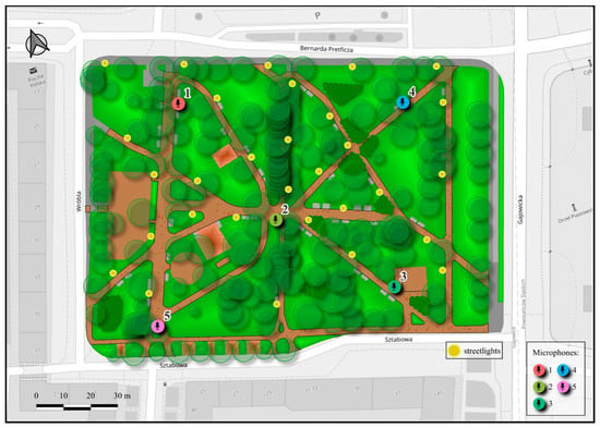
Field data were collected in Wrocław, the third-largest city in Poland by population. The city is situated in one of the country’s warmer regions and is characterised by relatively mild winters, warm summers, and substantial precipitation. Langiewicz Park is a small urban park (approx. 1.1 ha) located in the Gajowice district of Wrocław. The park was established in 1958 on the site of the former Gabitzer Friedhof. It is bounded by Gajowicka Street to the east, Bernarda Pretficza Street to the north, Wróbla Street to the west, and Sztabowa Street to the south. The park has a compact recreational layout (playground, outdoor gym, benches, and walking paths) and retains preserved old-growth trees. The surrounding district is subject to conservation protection as part of the city’s archaeological zone and historic urban layout (Figure 1). Land use around the park is multifunctional: to the north, there is a service area with a grocery market; to the west and south, multi-family residential development; and to the east, a facility with a military function. The location and spatial arrangement of Langiewicz Park indicate that it is a suitable study site for tracing soundscape patterns within a small urban park. The site was selected for comprehensive research within the URBIO BAUHAUS project, which aims to identify challenges associated with increasing biodiversity in cities. Recent work in the same park documents that users link lighting mainly to perceived safety and orientation, while also expressing strong concerns about biodiversity impacts and support for warmer-spectrum, targeted, and adaptive lighting strategies [15].

Figure 1. Langiewicz Park and its immediate surroundings.

2.2. Acoustic Sensor Network

Acoustic data were collected using AudioMoth recorders, selected for their compact form factor (58 mm × 48 mm × 15 mm) and suitability for unattended field deployment. Each unit contains an integrated analogue MEMS microphone and can record uncompressed audio to a microSD card across a wide range of sampling rates (8000–384,000 samples, s⁻¹, up to 384 kHz). Power was provided by AA batteries or rechargeable AA cells, allowing continuous field operation for up to 3 weeks under typical conditions. The devices include a real-time clock, enabling precise scheduling of pre-programmed recording windows. Device specifications are provided by Open Acoustic Devices in the AudioMoth documentation. During fieldwork, recorders were installed in dedicated AudioMoth IPX7 polycarbonate enclosures to protect the units against precipitation and moisture ingress.

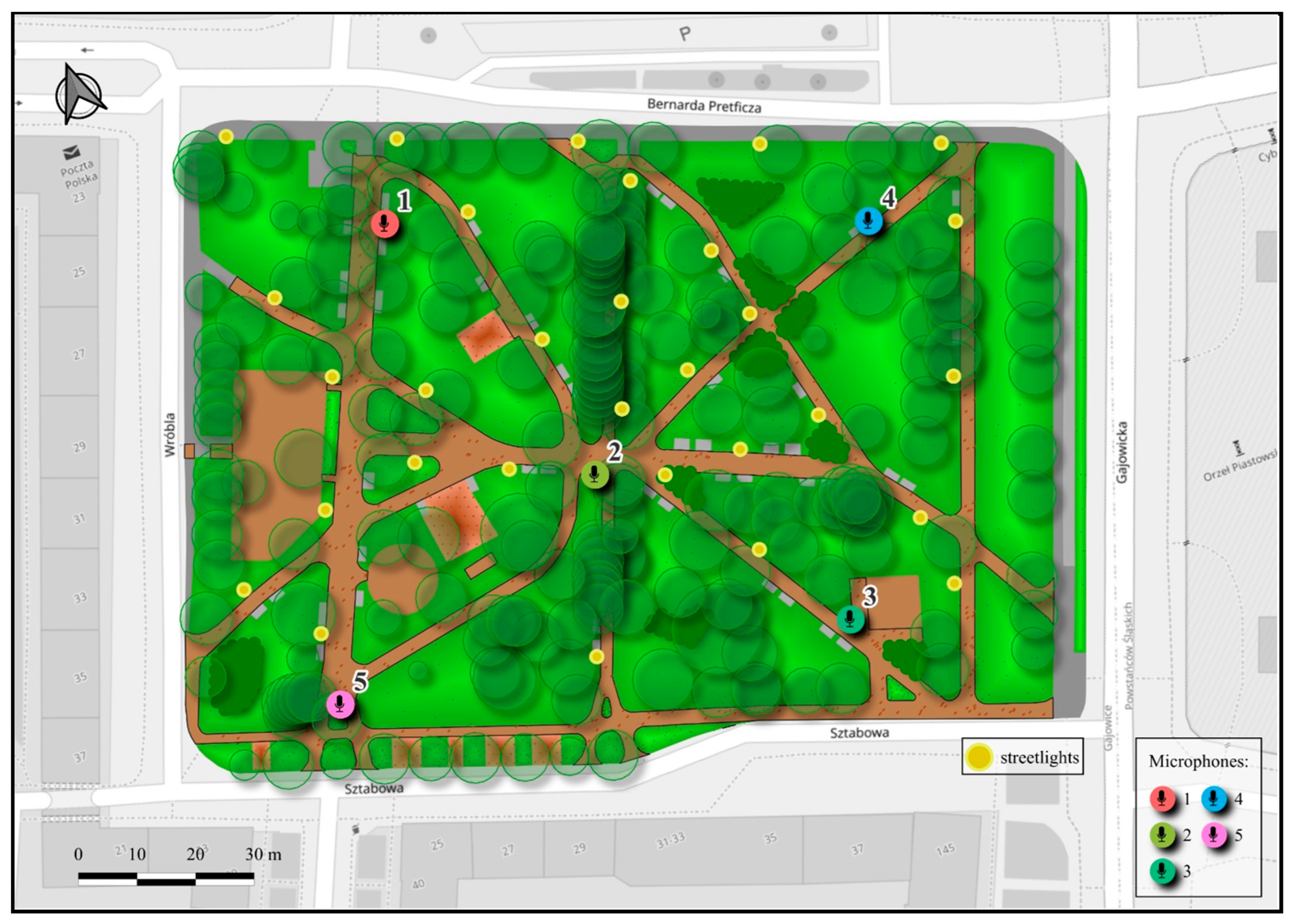
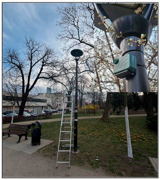
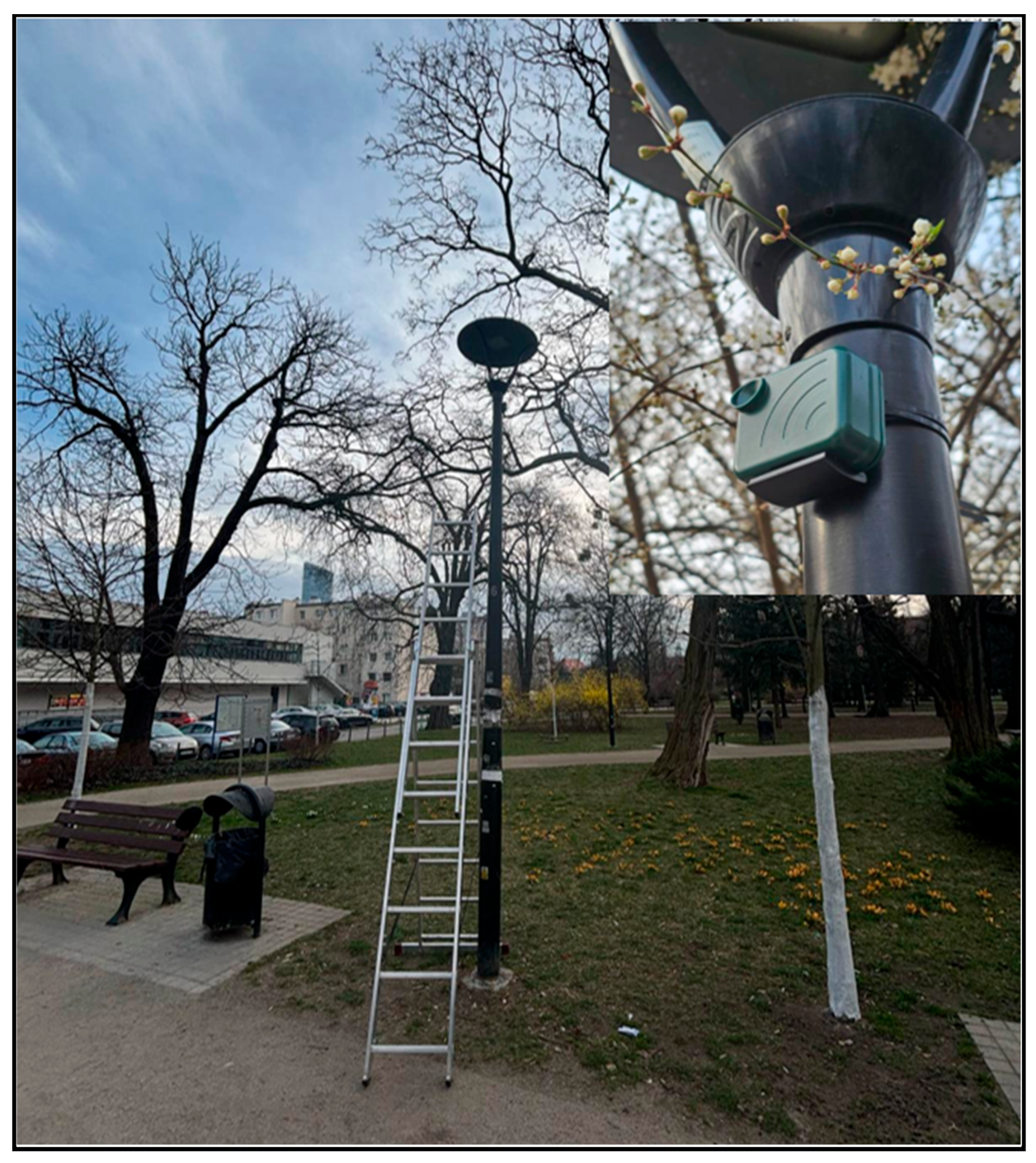
Five recorders were deployed within the park and mounted on lighting columns at a height of approximately 3.5 m. Inter-station spacing was approximately 50–70 m. All measurement locations were positioned adjacent to pedestrian paths; four were located close to the park corners, and one was placed in a central position to capture the interior soundscape (Figure 2).

Figure 2. Locations of the five passive acoustic monitoring stations (Mic 1−Mic 5) deployed in Langiewicz Park (≈1.1 ha), Wrocław. Monitoring points are shown relative to the park boundary and adjacent streets (Gajowicka Street, Bernarda Pretficza Street, Wróbla Street, and Sztabowa Street). One station (Mic 2) was placed in the park interior, and four stations were positioned near the corners to capture within-park spatial heterogeneity; inter-station spacing was approximately 50–70 m.

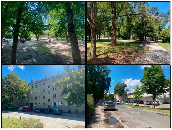
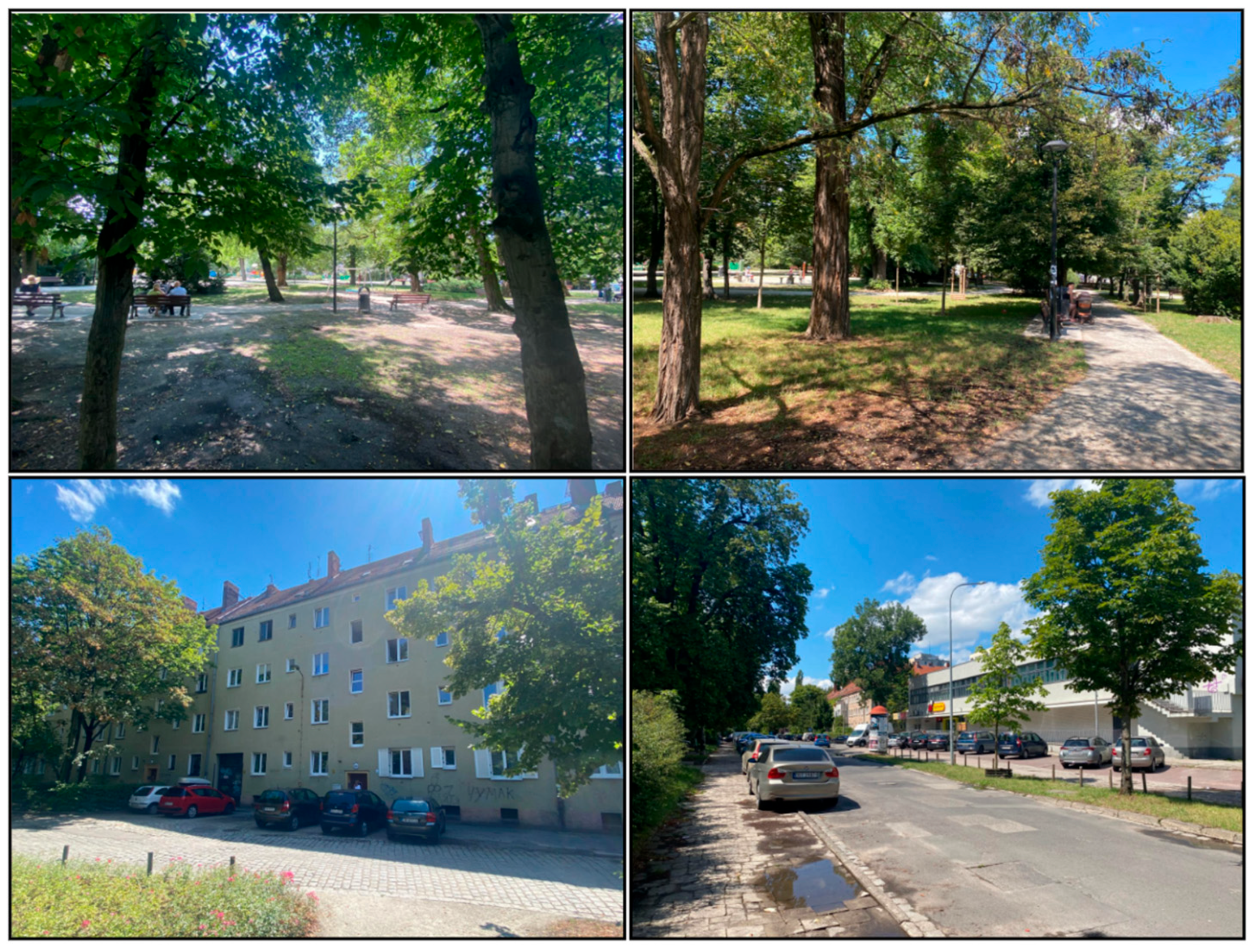
The five monitoring points were defined to reflect the park’s internal structure and the heterogeneity of its surroundings (Figure 3):

Figure 3. Microphone placement documented.

• Station 1 was located near a small greengrocer shop, by the path leading to the playground and towards the adjacent grocery market.
• Station 2 was situated in the central part of the park, at the intersection of several footpaths.
• Stations 3 and 4 were positioned along walking paths within the park.
• Station 5 was located along the same path corridor as Station 1.

A key criterion for selecting recorder locations was to achieve optimal acoustic coverage of the park area and to capture the broadest possible sample of sounds occurring within the park.

2.3. Recording Design and Temporal Coverage

Audio acquisition was organised into two field sessions. The first session ran from 13 to 20 March 2025 and the second from 22 to 23 April 2025. During both sessions, recorders operated continuously each day within a fixed nocturnal window, from 18:00 to 06:00, yielding uninterrupted nighttime sequences rather than block-sampled recordings. Recordings were stored as WAV files (Waveform Audio File Format) with 16-bit resolution. Two sampling frequencies were used during the campaign, 48,000 Hz and 250,000 Hz, reflecting parallel recording configurations applied within the study. Temporal coverage differed by month and by microphone location (Table 1). In March, stations Mic 2, Mic 3, Mic 4, and Mic 5 provided comparable recording volumes, each close to 74 h (range 74.05–74.83 h), whereas Mic 1 yielded 18.78 h. In April, exposure times were shorter across stations, ranging from 11.17 h (Mic 2) to 15.15 h (Mic 3). The total recording time exceeded 371 h. Continuity checks identified gaps attributable to technical failures. The most substantial loss occurred at Mic 4, which recorded no data in April (0.00 h). The reduced volume at Mic 1 in March, together with the shorter April series at the remaining stations, was linked to technical interruptions in recorder operation.

Table 1. Recording design and temporal coverage by monitoring stations during the two field sessions. For each microphone, the table reports the deployment dates and the total number of recorded hours within the nocturnal sampling window.

Mic.	Dates (March)	Hours	Dates (April)	Hours	Mic.
Mic. 1	14.03–20.03	18.78	22.04–23.04	15.12	Mic. 1
Mic. 2		74.83		11.17	Mic. 2
Mic. 3		74.05		15.15	Mic. 3
Mic. 4		74.40		0.00	Mic. 4
Mic. 5		74.45		13.43	Mic. 5
Total		361.51		55.4	Total

2.4. Signal Processing and Index Computation

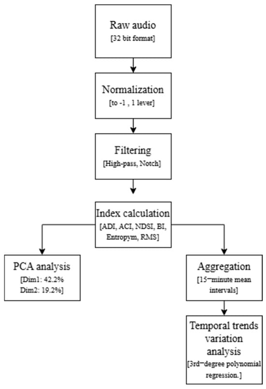
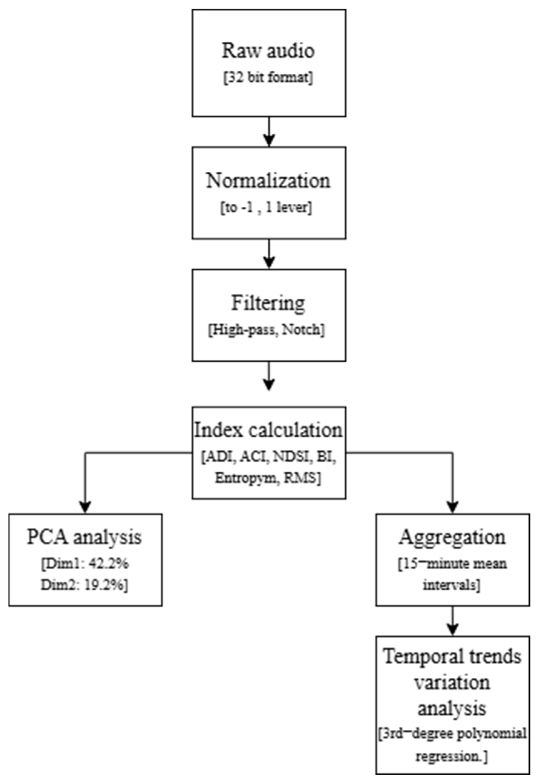
Audio signal processing followed a dual workflow (Figure 4), with methods selected to match the frequency range under analysis. The initial preprocessing included amplitude normalisation: raw recordings were converted to float32 and scaled to [−1, 1], where 0 represents the absence of acoustic events.

Figure 4. Signal processing and acoustic data analysis diagram.

For ultrasonic analysis targeting bat activity, the original files sampled at 250,000 Hz were retained. These recordings were filtered using a 4th-order Butterworth high-pass filter with a 25,000 Hz cut-off to isolate the ultrasonic band. In parallel, given the use of two sampling rates in the campaign, the sampling was standardised by decimating 250,000 Hz recordings to 48,000 Hz. This step was applied to make ecoacoustic indicators fully comparable across recordings with different input parameters.

Each recording was screened for technical artefacts associated with the mounting configuration. In the 18–24 kHz band, a recurrent noise component that originated from street lighting (transformers) was detected, with vibrations transmitted to the recorders through the lampposts. Where present, the artefact was treated using a notch filter, and affected fragments were removed, given their negative effect on acoustic index values. A digital filter was also applied to remove abrupt amplitude spikes. Events flagged in this way were labelled as “disturbances” and then checked manually to exclude signals that were not representative of the park’s environment.

Acoustic computations were implemented in Python using NumPy [16] and SciPy [17] for reading raw audio, normalisation, and calculation of the global RMS. The scipy.signal module was used for digital filtering (notch and Butterworth filters) and for power spectral density estimation using Welch’s method, which formed the basis for computing the NDSI, BI, ADI, and Entropy. Soundscape feature extraction used scikit-maad [18]: maad.sound was used to generate amplitude spectrograms, and the maad.feature was used to compute key indicators, including the ACI, ADI, BI, and Entropy. For the NDSI, frequency bands were defined as anthrophony: 1–2 kHz and biophony: 2–8 kHz. The same biophony band (2–8 kHz) was also used as the basis for calculating the bioacoustic index (BI).

Indices were calculated for the full duration of each recording, providing an integrated description of the park soundscape across the nocturnal monitoring window. Within the Welch estimator, a window length of 1024 samples was used; at 48,000 Hz, this reduces data volume through averaging without removing informative structure, which was important for time-efficient processing given the size of the dataset.

2.5. Data Preparation and Quality Control

Quality control was applied to all recordings admitted to analysis using rule-based digital screening. Segments were removed when the signal exceeded the admissible amplitude range at any point (clipping/overload). The same procedure was applied in cases of signal absence. Where technical noise was detected, the affected frequency range was removed. Zero-length audio files were identified automatically, excluded from the dataset, and omitted from downstream computations.

Prior to the analysis, the audio recordings were transformed to float32 and scaled to the range [−1, 1]. To produce figures showing index dynamics together with their variance, segment-level values were aggregated using the arithmetic mean. For multivariate analyses (PCA), the indices were further standardised to a mean of 0 and a standard deviation of 1, aligning variables measured on different numeric scales. After quality filtering, 22,284 out of 28,915 verified files passed the control procedure and were retained for subsequent analyses.

2.6. Statistical Analysis

The analyses followed three complementary steps: (i) the description of nocturnal index trajectories using time-trend models, (ii) the comparison between microphone locations and months using distributional summaries, and (iii) multivariate ordination employed to assess co-variation among indices and to test for within-park acoustic heterogeneity.

The nocturnal soundscape dynamics were modelled using third-degree polynomial trend functions, selected to capture cyclic structure in evening and dawn periods. The comparisons across locations (Mic 1–Mic 5) and months (March vs. April) were conducted through the analysis of statistical distributions, visualised with violin plots. To evaluate co-variation among indices and to support inference on acoustic heterogeneity within the park, principal component analysis (PCA) was performed, allowing the identification of distinct acoustic signatures associated with individual monitoring stations.

All analyses of index dynamics and variance were carried out on data aggregated to 15 min time series. For the temporal trend models, the optimal polynomial degree for each microphone (and index) was selected using AICc, favouring models that balance goodness-of-fit with parsimony. Model performance was summarised using the adjusted coefficient of determination (adjusted R²). Model validity was assessed via residual diagnostics, including checks of distributional normality and homogeneity of variance.

Signal preprocessing (amplitude normalisation, decimation from 250 kHz to 48 kHz, and digital filtering with notch and Butterworth filters) and computation of the raw acoustic indices were conducted in Python 3.12. Statistical modelling (AICc-based trend modelling), data standardisation, PCA, and final figure generation were performed in R 4.5.1.

3. Results

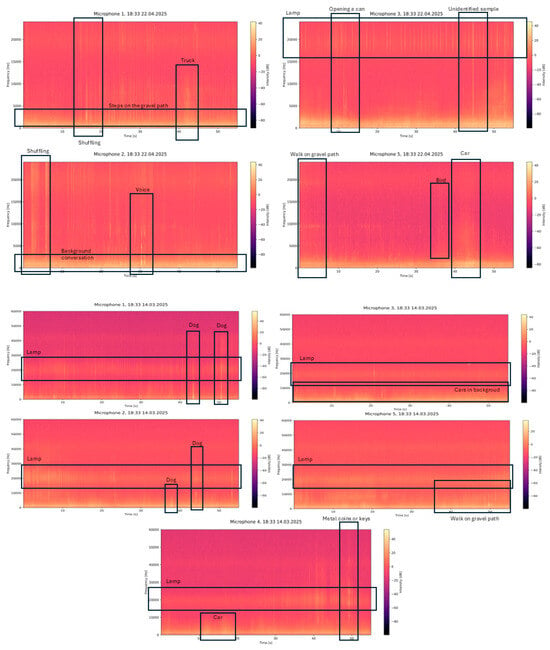
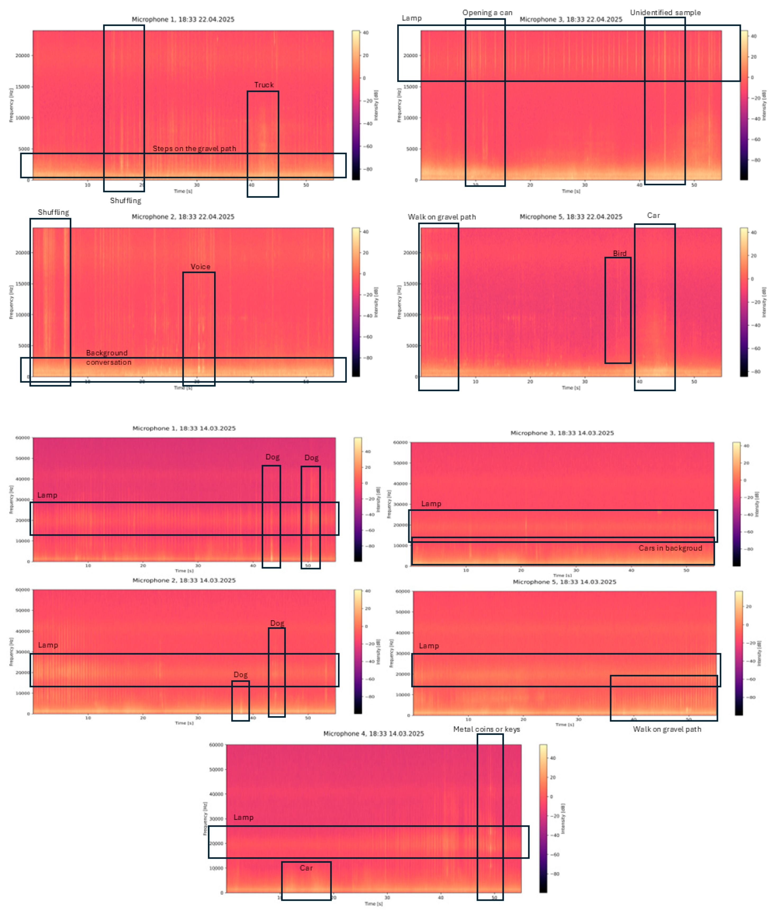
The analysis covers the evening and nighttime period (18:00–06:00) across five monitoring locations (Mic 1–Mic 5) during March and April 2025. During the inspection of recordings from 14 March at 18:33 (Figure 5), a recurrent vibration-related artefact was visible around ~20 kHz, consistent with mechanical vibrations transferred to the recorders by transformers in street lighting. In the same interval, sound events representative of typical park use were detected, including dog barking (Mic 1 and Mic 2), walking on gravel paths (Mic 5), and intense vehicle traffic (Mic 3). Spring recordings from 22 April at 18:30 (Figure 5) broadened the observed pool of acoustic phenomena. The dataset includes conversations (Mic 2), walking on paths (Mic 1), scuffing/shuffling sounds on hard surfaces (Mic 3), and biological events such as birdsong (Mic 5). Across both sessions, these examples illustrate that the recorders captured zone-specific acoustic events while maintaining continuity of monitoring within the predefined time window.

Figure 5. Spectra are displayed up to 60 kHz (March) and 24 kHz (April). Black rectangles indicate acoustically distinct events used for qualitative interpretation and a recurrent narrow-band component around ~20 kHz attributed to street lighting transformers transmitted via mounting structures.

3.1. Overview of Index Distributions and Temporal Coverage

Descriptive statistics of the ecoacoustic indices show within-park spatial heterogeneity at the microscale. Index values vary across microphone locations and between the two sampling periods, as reflected by the median, interquartile range (25–75%), and mean ± standard deviation reported in Table 2 (March) and Table 3 (April).

Table 2. Summary of ecoacoustic indices in March 2025 for Mic 1–Mic 5, reported as median [IQR]; mean ± SD. NDSI used 2–8 kHz (biophony) and 1–2 kHz (anthropophony) bands; BI integration range 2–8 kHz.

Mic.	RMS_Global	NDSI	ACI (×10−4)	ADI	BI	Entropy
	(Med [IQR]; Mean ± SD)
Mic. 1	0.02	−0.34	1.10	2.91	5.65	0.46
	[0.01–0.03]	[−0.52–−0.07]	[1.08–1.12]	[2.58–2.98]	[4.22–7.39]	[0.41–0.51]
	0.02 ± 0.01	−0.26 ± 0.36	1.10 ± 0.03	2.67 ± 0.50	6.05 ± 2.72	0.46 ± 0.08
Mic. 2	0.02	−0.45	1.08	2.95	5.15	0.49
	[0.01–0.03]	[−0.59–−0.13]	[1.08–1.11]	[2.76–2.99]	[2.99–7.17]	[0.43–0.54]
	0.02 ± 0.01	−0.32 ± 0.37	1.10 ± 0.0	2.76 ± 0.4	5.43 ± 3.20	0.48 ± 0.10
Mic. 3	0.02	−0.57	1.08	2.87	6.85	0.48
	[0.01–0.03]	[−0.66–−0.33]	[1.08–1.10]	[2.52–2.98]	[3.61–9.95]	[0.44–0.52]
	0.03 ± 0.02	−0.42 ± 0.36	1.10 ± 0.03	2.62 ± 0.57	6.91 ± 3.99	0.48 ± 0.09
Mic. 4	0.02	−0.58	1.08	2.89	7.95	0.46
	[0.01–0.04]	[−0.65–−0.41]	[1.08–1.09]	[2.59–2.98]	[4.50–10.70]	[0.42–0.51]
	0.03 ± 0.02	−0.45 ± 0.32	1.09 ± 0.03	2.63 ± 0.59	7.71 ± 3.97	0.46 ± 0.10
Mic. 5	0.02	−0.44	1.08	2.94	4.01	0.49
	[0.01–0.03]	[−0.62–−0.10]	[1.08–1.10]	[2.60–2.99]	[2.34–5.89]	[0.43–0.55]
	0.02 ± 0.03	−0.33 ± 0.39	1.10 ± 0.03	2.65 ± 0.58	4.43 ± 2.61	0.48 ± 0.10

Table 3. Summary of ecoacoustic indices in April 2025 for Mic 1–Mic 5, reported as median [IQR]; mean ± SD. NDSI used 2–8 kHz (biophony) and 1–2 kHz (anthropophony) bands; BI integration range 2–8 kHz.

Mic.	RMS_Global	NDSI	ACI (×10−4)	ADI	BI	Entropy
	(Med [IQR]; Mean ± SD)
Mic. 1	0.017	−0.28	1.14	2.76	7.96	0.49
	[0.009–0.024]	[−0.46–−0.03]	[1.12–1.16]	[2.42–2.97]	[5.63–10.51]	[0.41–0.55]
	0.018 ± 0.011	−0.23 ± 0.33	1.16 ± 0.05	2.61 ± 0.45	8.61 ± 4.38	0.47 ± 0.10
Mic. 2	0.015	−0.34	1.13	2.80	6.40	0.52
	[0.008–0.024]	[−0.56–−0.03]	[1.12–1.16]	[2.41–2.98]	[3.56–9.97]	[0.44–0.57]
	0.017 ± 0.010	−0.26 ± 0.37	1.15 ± 0.04	2.62 ± 0.46	7.64 ± 5.33	0.50 ± 0.09
Mic. 3	0.023	−0.62	1.14	2.55	10.23	0.49
	[0.013–0.034]	[−0.70–−0.45]	[1.13–1.17]	[2.23–2.87]	[6.90–13.17]	[0.45–0.52]
	0.025 ± 0.014	−0.52 ± 0.27	1.16 ± 0.04	2.50 ± 0.42	9.95 ± 4.89	0.48 ± 0.07
Mic. 5	0.018	−0.38	1.13	2.61	7.34	0.51
	[0.008–0.028]	[−0.58–−0.10]	[1.12–1.16]	[2.21–2.97]	[3.91–9.95]	[0.45–0.56]
	0.019 ± 0.014	0.31 ± 0.33	1.15 ± 0.03	2.49 ± 0.53	7.60 ± 4.33	0.50 ± 0.09

In March, indices showed relative spatial stability across most parameters, with the exception of BI, which exhibited localised peaks in biological activity. The NDSI remained consistently negative at all stations, reflecting a dominant technophonic background.

In April, the data showed a significant seasonal change (Table 3), characterised by an overall increase in the ACI and BI. Mic 3 proved to be a highly productive anomaly, characterised by maximum biological activity but minimal spectral diversity (ADI) and balance (NDSI). In contrast, Mic 2 combined the lowest signal energy with the highest diversity. Local variance analysis also revealed extreme variability characteristic of a given location in Mic 5, which remained undetected by global average trends.

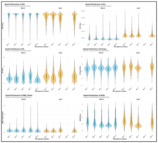
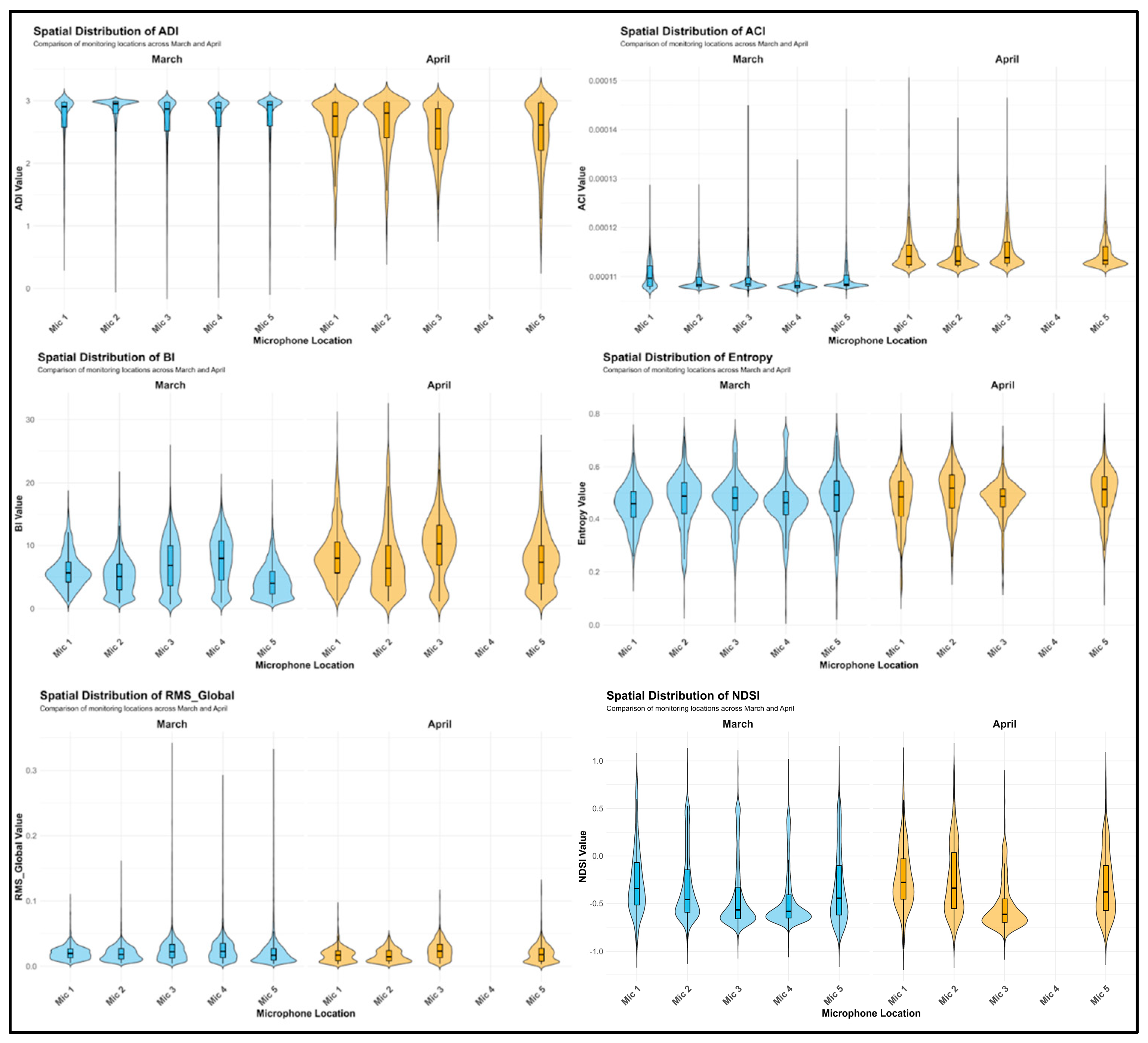
The distribution plots (Figure 6) confirm that statistical distributions are not homogeneous across the five locations for most indices. The NDSI exhibits the strongest spatial variability. In March, medians for Mic 1, Mic 2, and Mic 4 cluster around approximately −0.5, while Mic 5 shows a broader distribution. In April, between-microphone differences increased, with Mic 3 showing a stronger low-frequency dominance, while Mic 1 and Mic 5 registered higher contributions from higher-frequency bands.

Figure 6. Spatial distributions of six ecoacoustic indices across the five monitoring locations in Langiewicz Park, Wrocław shown separately for the March (blue) and April (yellow) campaigns. Panels report the ADI, ACI, BI, Entropy, RMS_Global, and NDSI. Violin shapes represent the kernel density of 15 min aggregated index values; embedded boxplots show the median and interquartile range (IQR). Mic 4 has no April distribution due to missing recordings in that session.

ACI also differs across locations. In April, Mic 3 and Mic 5 reach higher medians than Mic 1 and Mic 2. The distribution width at Mic 1 is larger than at Mic 5, indicating different magnitudes of variability in short-term sound dynamics within the same time window. For the BI, the highest intensity in April occurs at Mic 3, while the remaining microphones show distinct distribution shapes and ranges of extreme values. The ADI and Entropy are the most similar across locations, with the ADI remaining between 2.5 and 3.0, and Entropy fluctuating around 0.5 at all stations. RMS_Global shows a comparable profile at each microphone, characterised by low baseline values with sporadic amplitude spikes.

Across indices, shifts in distribution are not uniform across monitoring points. The median shift in the ACI at Mic 1 is more pronounced than at Mic 5, and the differences in the shape of the distributions across microphones indicate that each recorder captured a distinct acoustic character of its local surroundings, despite simultaneous operation within the same park.

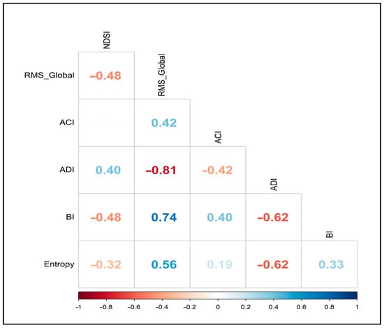
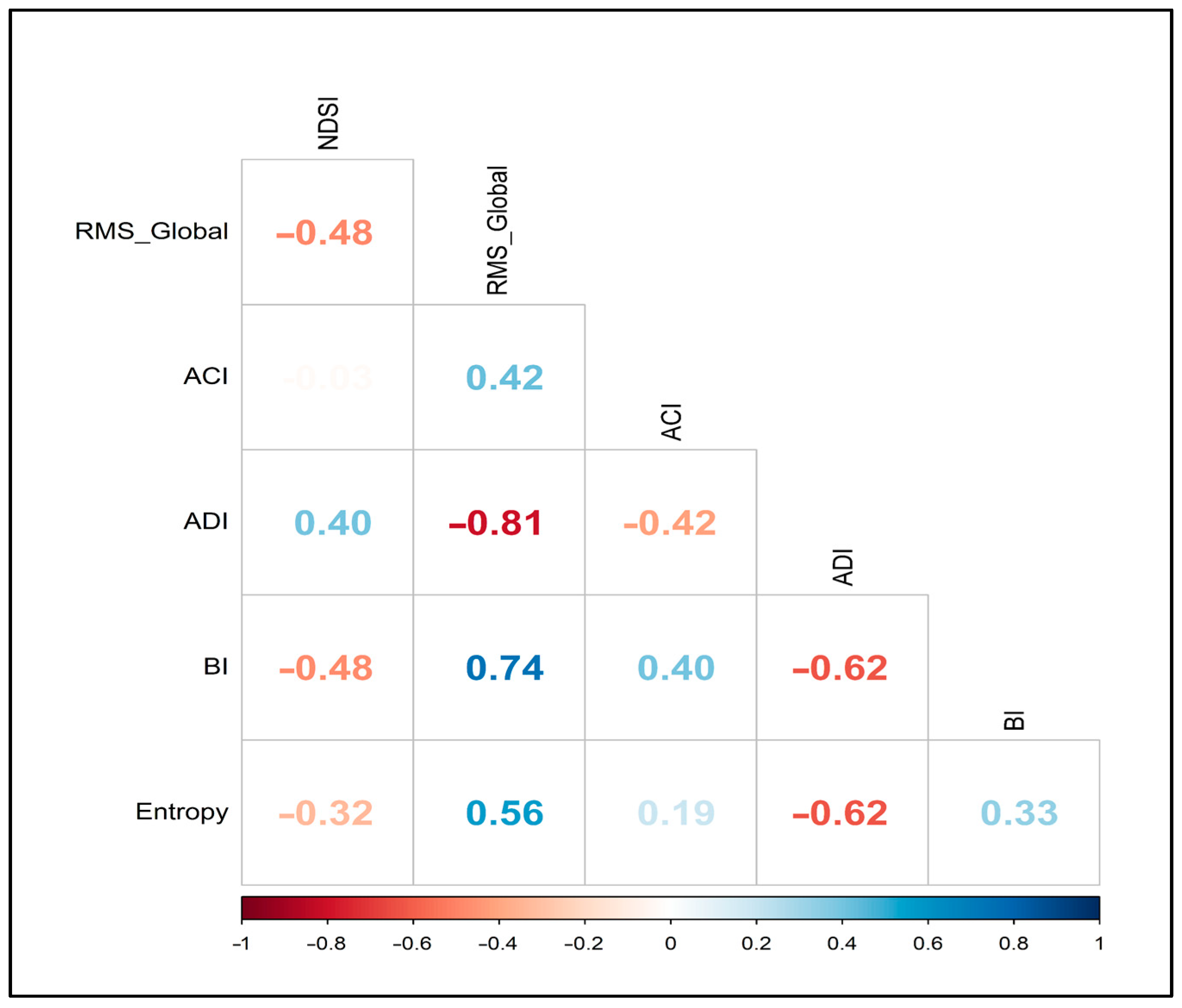
The correlation analysis (Figure 7) indicates structured dependence among the six ecoacoustic indices, supporting a compact description of nocturnal soundscape dynamics in the park. The matrix shows a strong relationship between overall acoustic energy and indices capturing soundscape structure. RMS_Global is strongly negatively correlated with the ADI, indicating that increases in total signal energy coincide with lower detected diversity across frequency bands. The NDSI exhibits a distinct profile compared with the remaining indices: it correlates positively only with the ADI, while showing negative correlations with the other indicators. In these data, stronger low-frequency dominance is associated with higher overall acoustic energy. The ACI shows a moderate but clear association with the BI and RMS_Global, consistent with higher short-term amplitude dynamics occurring under higher total energy and stronger biological activity. At the same time, the ACI remains close to independent from the NDSI, suggesting that impulsive/rapid signal structure varies largely independently of whether the soundscape is dominated by biological or anthropogenic components, as captured by the NDSI. The relationships among Entropy, ADI, and BI indicate that higher Entropy coincides with lower ADI values and higher BI values, reflecting a joint pattern in which more complex, less ordered signals align with stronger bioacoustic energy in this setting.

Figure 7. Pairwise correlation matrix for the six ecoacoustic indices computed from the nocturnal recordings across all monitoring locations and both sampling periods in Langiewicz Park, Wrocław. Values are Pearson correlation coefficients (r), with colour indicating direction and magnitude (red = negative, blue = positive). The strongest associations include a negative relationship between RMS_Global and ADI (r = −0.81) and a positive relationship between RMS_Global and BI (r = 0.74).

3.2. Nocturnal Temporal Trends Variation

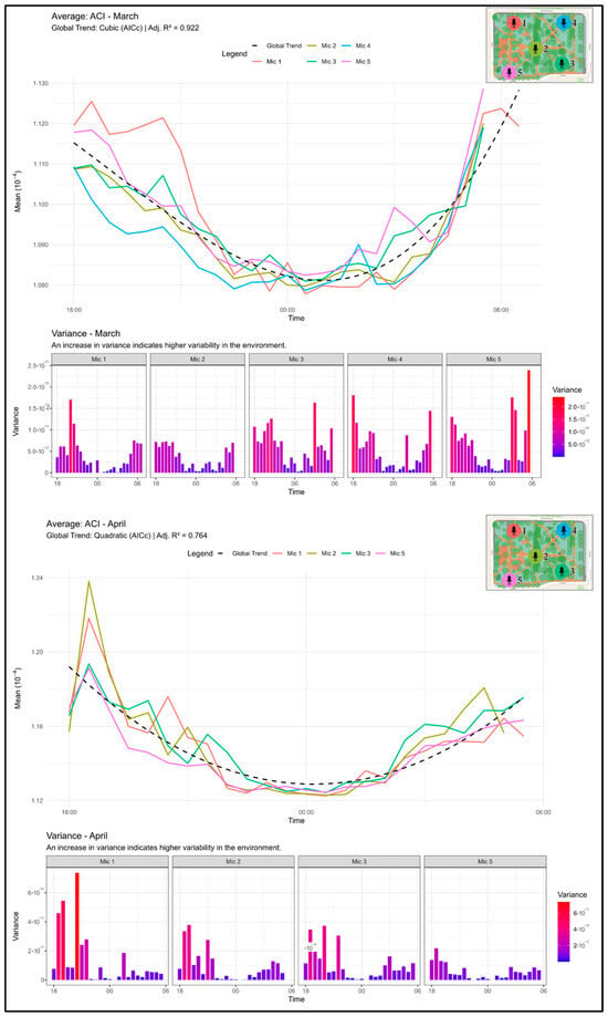
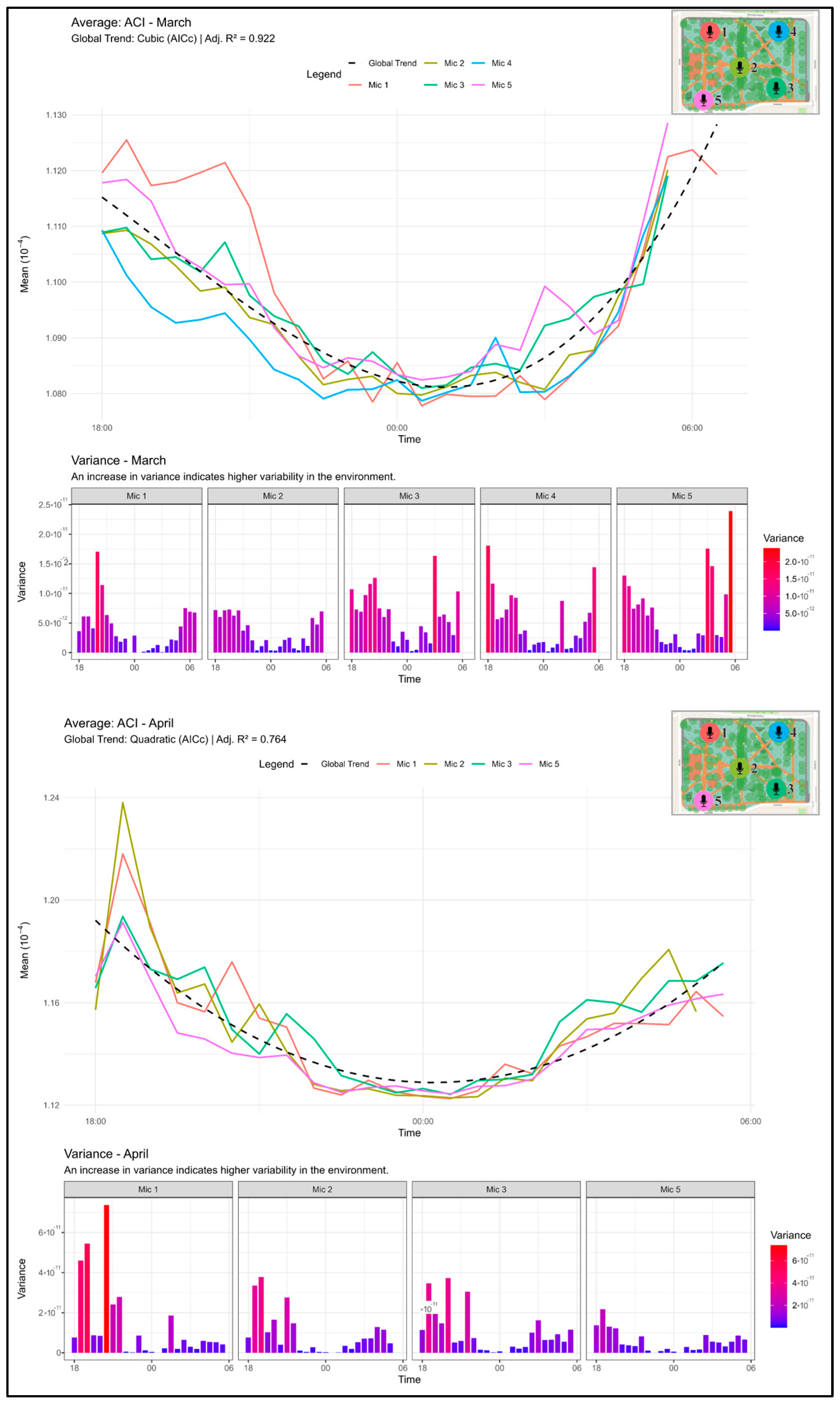
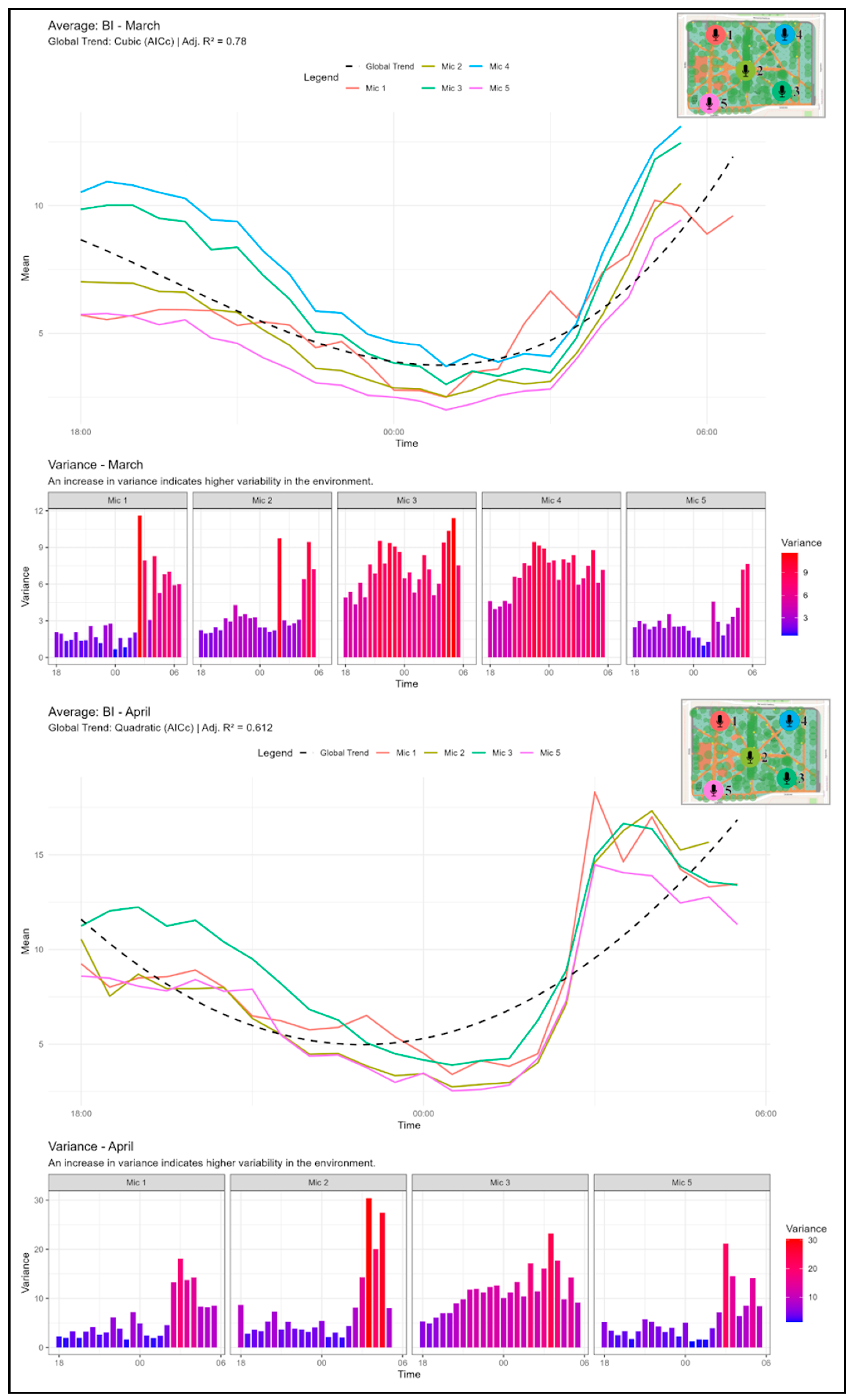
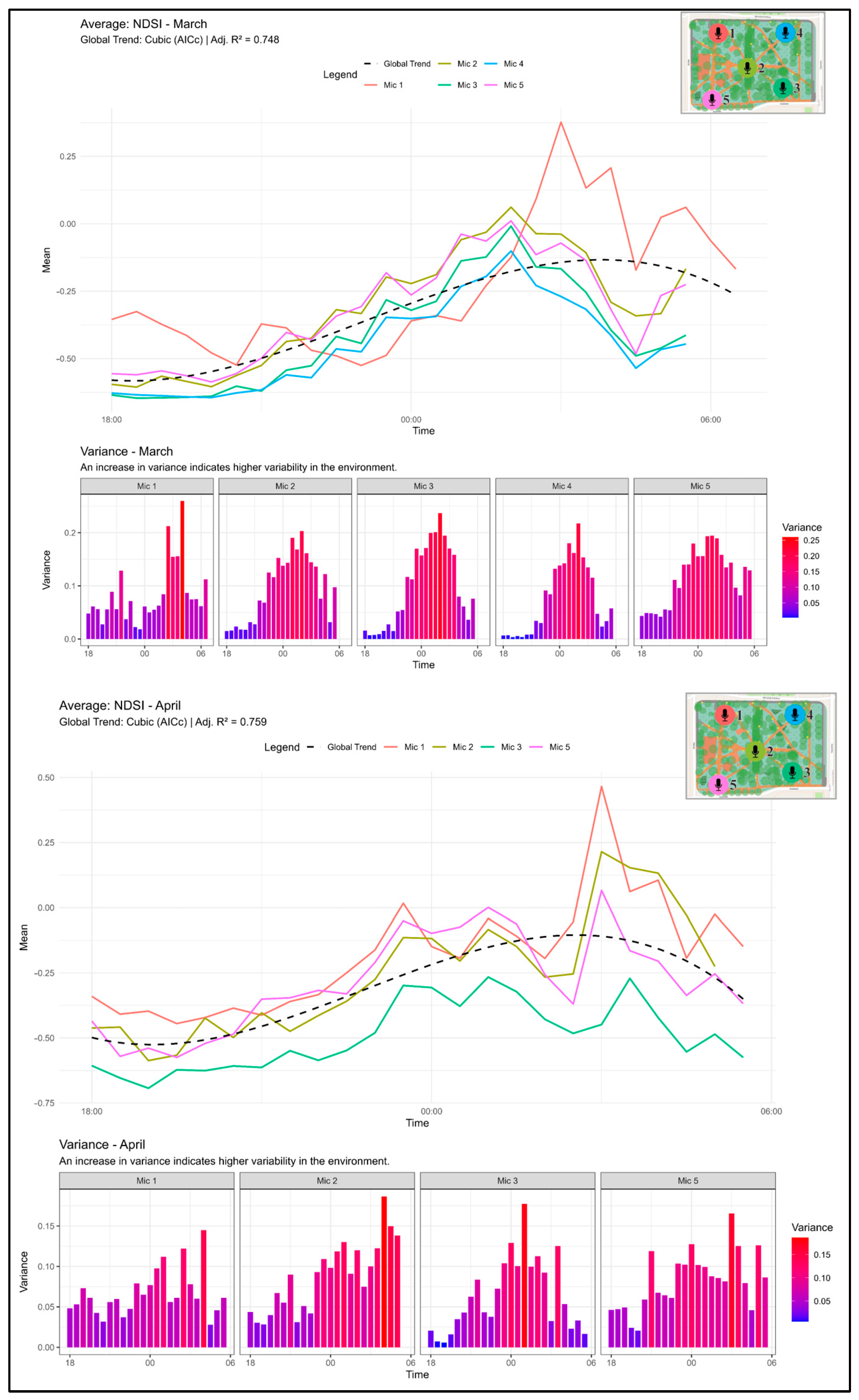
Time-series modelling for the 18:00–06:00 window shows that the nocturnal index dynamics are tightly linked to the daily cycle and to transitional phase windows (dusk and dawn). Using the AICc for model selection yielded non-linear regression fits with high explanatory power (adjusted R² = 0.44–0.93). Across microphones, three dominant global trend types were identified from the fitted regression curves (Figure 8, Figure 9 and Figure 10):

Figure 8. Nocturnal variation in the acoustic complexity index (ACI) across five monitoring locations in Langiewicz Park, Wrocław during the March and April 2025 campaigns. Line plots show mean ACI values aggregated to 15 min intervals for each microphone together with the pooled global trend fitted using polynomial regression; the selected model form (AICc) and adjusted R² are reported in the panel headers. Insets indicate the spatial configuration of microphones. Bar charts summarise the within-bin variance in ACI for each microphone across the same time window, with colour intensity reflecting variance magnitude and highlighting time periods of elevated short-term variability. Mic 4 is absent in April due to missing recordings.

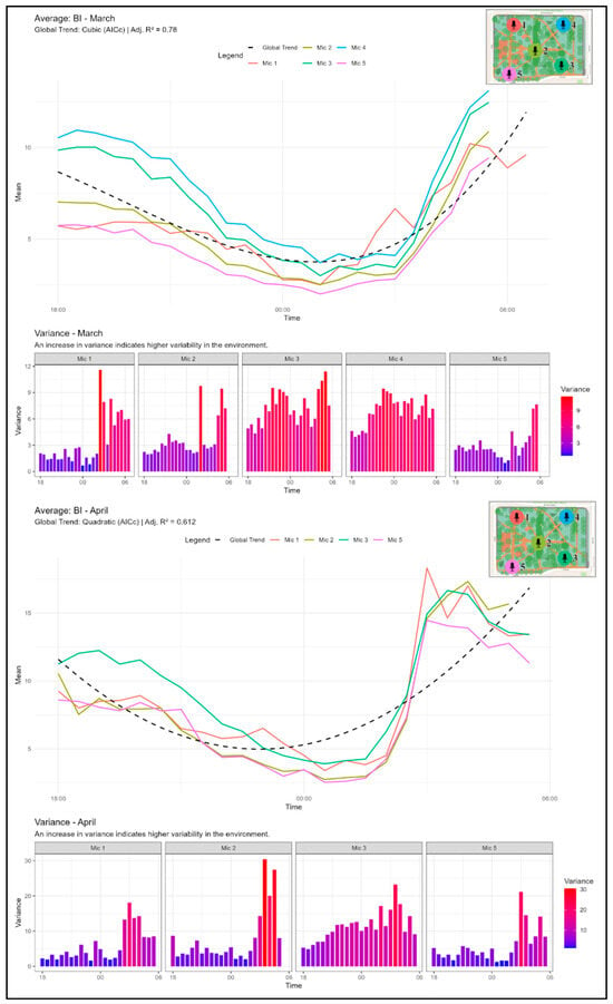
Figure 9. Nocturnal variation in the bioacoustic index (BI) across five monitoring locations in Langiewicz Park, Wrocław during the March and April 2025 campaigns. Line plots show mean BI values aggregated to 15 min intervals for each microphone together with the pooled global trend fitted using polynomial regression; the selected model form (AICc) and adjusted R² are reported in the panel headers. Insets show the spatial configuration of microphones. Bar charts report the within-bin variance of BI at each microphone across the same time window, with colour intensity indicating variance magnitude and highlighting periods of increased biological acoustic activity and/or intermittent events. Mic 4 is absent in April due to missing recordings.

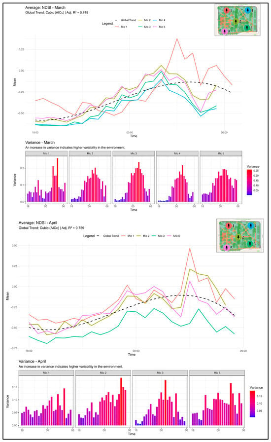
Figure 10. Nocturnal variation in the normalised difference soundscape index (NDSI) across five monitoring locations in Langiewicz Park, Wrocław during the March and April 2025 campaigns. Line plots show mean NDSI values aggregated to 15 min intervals for each microphone together with the pooled global trend fitted using AICc-selected polynomial regression; model form and adjusted R² are reported in the panel headers. Insets indicate the microphone layout. Bar charts report the within-bin variance of NDSI for each microphone over the same nocturnal window, with colour intensity indicating variance magnitude and highlighting periods when the balance between the anthrophony (1–2 kHz) and biophony (2–8 kHz) band shifts more strongly. Mic 4 is absent in April due to missing recordings.

• U-shaped trajectories were observed for the ACI, Entropy, and RMS_Global. These indices decline after sunset, reach minima around 00:00–02:00, then increase sharply during the dawn window.
• Cubic (asymmetric) trajectories characterise the NDSI and BI, showing different curve slopes after sunset than before dawn, which indicates asymmetry between the evening and morning dynamics. In April, the NDSI trend indicates a progressive shift across the night towards stronger biological band contribution relative to the anthropogenic band definition used in NDSI.
• Inverted U-shaped trajectories are associated with the ADI, with peak frequency-band diversity around the middle of the night, coinciding with reduced loudness. Increases in the ADI co-occur with low RMS_Global values during nocturnal hours.

To test whether the global trend adequately represents local dynamics, local slope behaviour was examined using a Taylor series interpretation of the fitted trend within 40 min windows after sunset and after sunrise. This highlights meaningful between-microphone differences: a shared global mean trend does not translate into consistent local directional coefficients across sensors, supporting a lack of acoustic uniformity within the park.

Variance patterns reinforce this point. Increased variance within specific time windows indicates higher local variability and the presence of intermittent point events. A clear dawn window is visible around 04:00–05:30, where the BI shows pronounced variance spikes at Mic 2 in April, while Mic 5 remains comparatively stable. A dusk window is also evident around 18:00–19:30, where the ACI shows high variance at Mic 1 in March that is not mirrored at Mic 2.

3.3. Multivariate Ecoacoustic Space

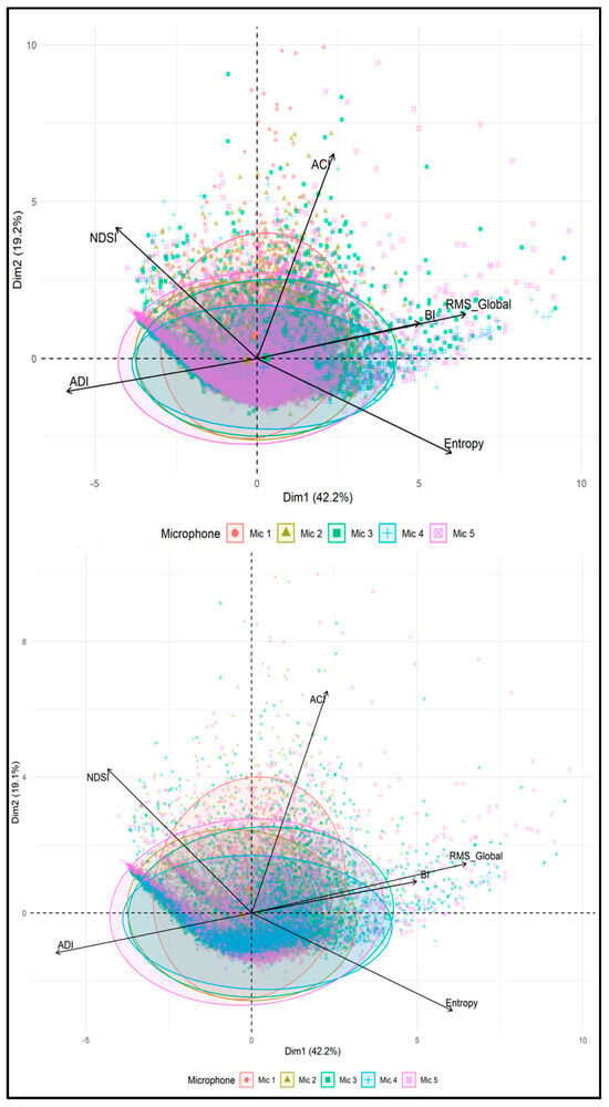
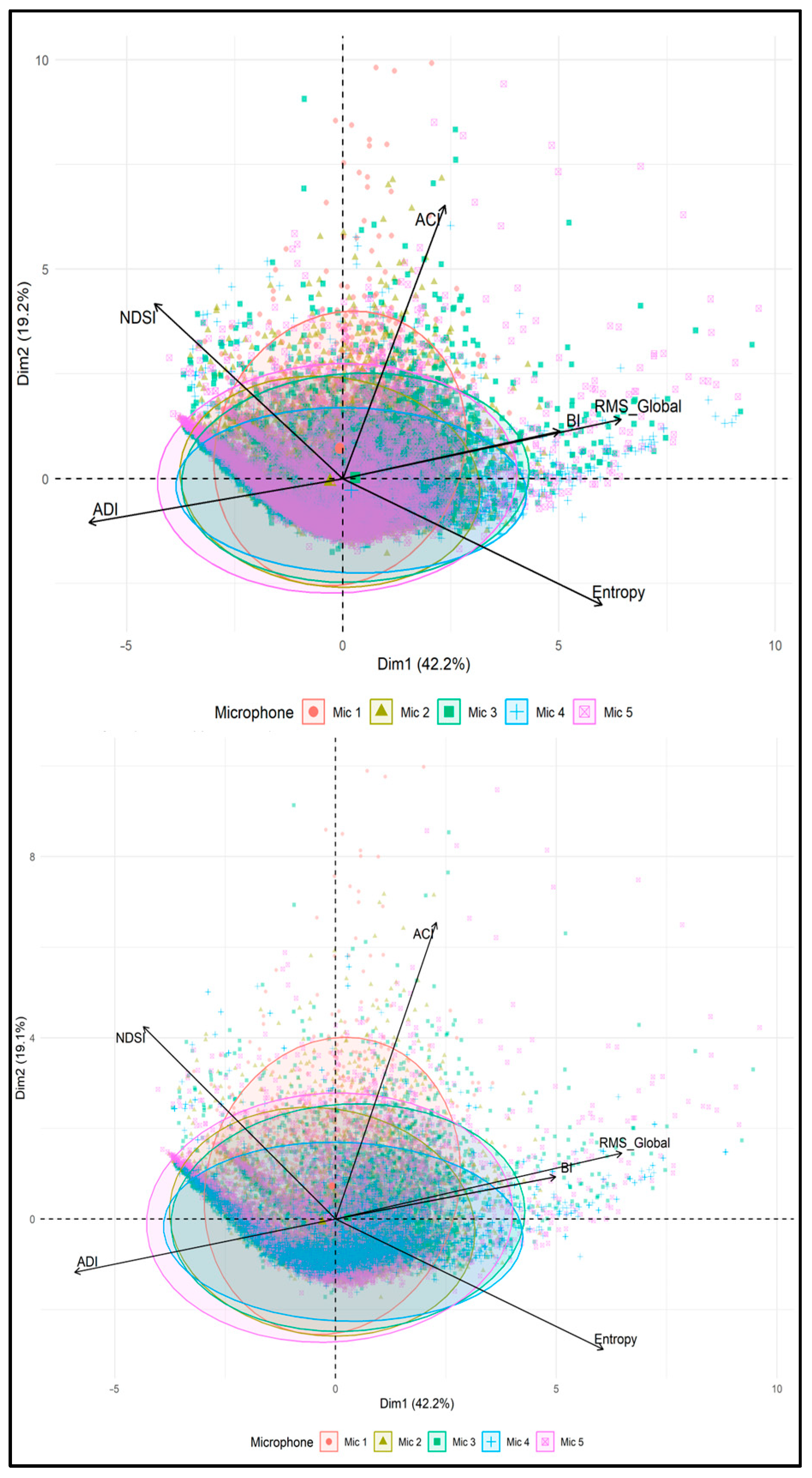
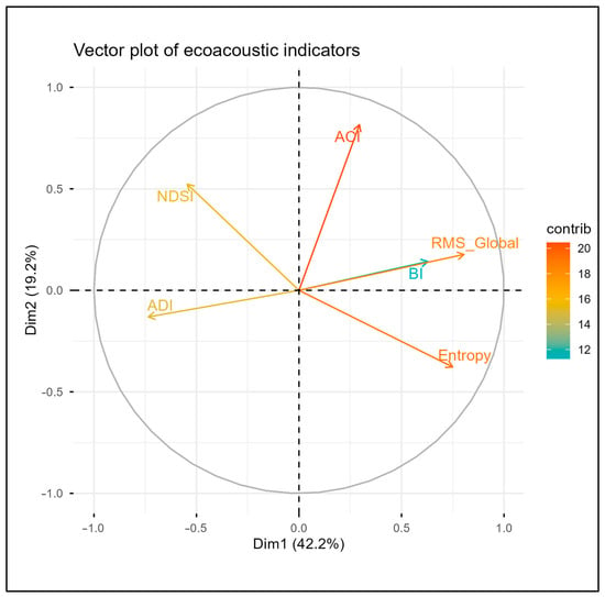
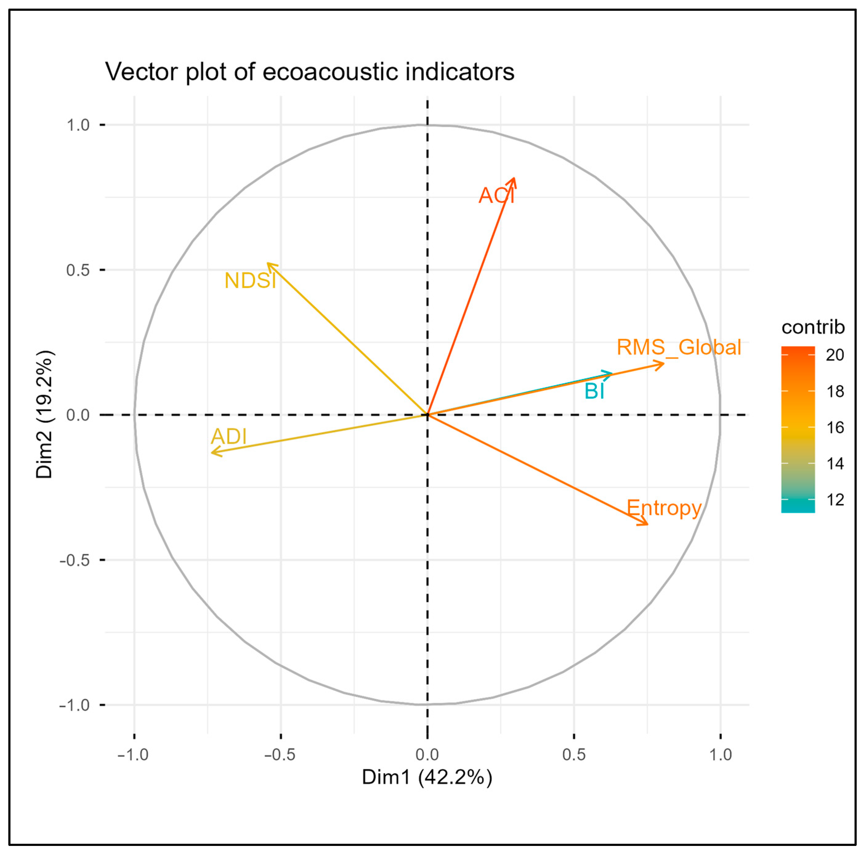
Principal component analysis (PCA) was used to summarise the joint variability of the six ecoacoustic indices in a low-dimensional space. The first two dimensions explained 61.4% of total variance (Dim1: 42.2%, Dim2: 19.2%). The first component (Dim1) represents a dominant gradient defined by strong positive loadings for RMS_Global, the BI, and Entropy, paired with a strong negative loading for the ADI. In the ordination (Figure 10), these variables align in opposing directions along the horizontal axis, indicating that periods or locations characterised by higher acoustic energy and bioacoustic band activity tend to coincide with lower acoustic diversity as captured by the ADI. The second component (Dim2) is driven mainly by the ACI, whose vector is oriented close to orthogonal relative to Dim1 (Figure 11). This configuration indicates that short-term temporal variability captured by the ACI forms a largely independent axis, separate from the dominant energy/bioacoustic gradient (Figure 12). To assess robustness to missing data, a sensitivity analysis was performed by comparing the PCA structure excluding Mic 4 (Figure 11, upper) with the version including simulated data for this location (Figure 11, lower). The results indicate high structural stability; the orientations of the indicator vectors and the distribution of monitoring points remain almost identical in both configurations, and the total variance explained differs by only 0.1% (61.4% compared to 61.3%). This confirms that the technical failure in Mic 4 did not significantly affect the global multidimensional characteristics of the park’s soundscape.

Figure 11. PCA biplots demonstrating robustness: original dataset excluding Mic 4 due to technical failure (upper) versus sensitivity analysis incorporating simulated data for this location (lower). Nearly identical indicator loadings and dispersion confirm the structural stability of the multivariate space despite missing records. Dim1: 42.2% and Dim2: 19.2% explain approximately 61.4% of total variance in both configurations.

Figure 12. PCA variable correlation circle showing the loadings of the six ecoacoustic indices (RMS_Global, NDSI, ACI, ADI, BI, and Entropy) on the first two principal components computed from nocturnal recordings across all monitoring locations in Langiewicz Park, Wrocław. Arrow direction indicates the sign of each loading, arrow length indicates the strength of association with the PCA axes, and colour denotes the relative contribution of each variable to the ordination. Dim1 and Dim2 explain 42.2% and 19.2% of total variance, respectively.

4. Discussion

4.1. Fine-Scale Heterogeneity Inside a Single Urban Park

The results indicate clear differences among the five microphones, supporting the presence of acoustically distinct zones within a single, small urban park. The PCA ordination shows a broad spread of observations across microphones, indicating that the park cannot be treated as acoustically homogeneous even at short inter-sensor distances. The micro-scale divergence is well-illustrated by Mic 2, which consistently recorded among the highest mean values of the ACI and elevated Entropy in April, alongside the highest variance in the ACI and the second-highest variance in Entropy. Taken together, this pattern suggests a location with high short-term acoustic complexity and structural variability, compatible with a localised hotspot of biological activity and mixed sound sources. Variance is interpreted here as an indicator of instability in the local acoustic environment, reflecting intermittent events and rapidly changing sound conditions rather than a stationary background.

Spatial heterogeneity is also evident in the distribution of overall sound energy. In April, Mic 5 exhibited the strongest early morning variance in RMS_Global, consistent with episodic anthropogenic contributions such as delivery vehicles or incidental road noise from the adjacent residential area and nearby market. The variability of biophony was similarly non-uniform: in April, Mic 2 showed the largest BI variance peak shortly before 06:00, indicating that the dawn chorus intensity was most variable, or most intermittently amplified, at this station.

The analysis of the shape of distributions (Figure 5) and variance (Figure 7, Figure 8 and Figure 9) allows for precise identification of micro-zones within the park. Wide NDSI profiles on the outskirts indicate an unstable acoustic background, while the interior of the park is characterised by more concentrated distributions. Variance spikes in the dawn window (04:00–06:00) document the transition from constant noise to intense, intermittent biological events. In turn, the inverted ADI trajectory confirms that the highest spectral diversity occurs at the lowest total energy. This is due to the reduction in dominant low-frequency noise, which allows for a more even distribution of energy across the bands.

These within-park contrasts underline why single-point monitoring risks under-sampling local soundscape dynamics. Even when global nocturnal trends are shared across stations, local mean levels and short-term variance differ in ways that are ecologically and methodologically relevant for interpreting soundscape structure at fine spatial scales. Vegetation structure can contribute to these patterns by shaping habitat suitability and acoustic transmission, with tree and shrub cover supporting distinct animal assemblages and modifying sound propagation [19]. Vegetation elements such as trees, hedges, and dense shrubs can also support the formation of quieter subzones by increasing surface roughness and attenuating urban noise more effectively than open grassed areas [20]. However, these spatial contrasts are not static and undergo significant changes when analysed at different time scales, as described in detail in the next section.

4.2. Seasonal and Nocturnal Ecoacoustic Phenology

Time-series patterns point to a pronounced nocturnal cycle shaped by the interaction between urban activity and biological signalling. Sound energy metrics (RMS_Global) and the bioacoustic index (BI) follow a characteristic U-shaped trajectory, with values declining after dusk and reaching their minimum between 22:00 and 03:00. This trough is consistent with reduced traffic flow along adjacent streets (e.g., Gajowicka and Sztabowa) and a broader decline in evening anthropogenic activity. The resulting reduction in low-frequency background sound improves the detectability of biological signals that are commonly masked during periods of higher anthrophony. The evidence of behavioural adjustment to this masking regime has been reported in urban birds, with nocturnal singing occurring more frequently under high daytime noise exposure [21].

Acoustic diversity responds differently to this nocturnal quietening. The acoustic diversity index (ADI) exhibits an inverted-U trajectory, with diversity peaking in the middle of the night despite lower overall acoustic energy. As dominant, broadband transport noise diminishes, the remaining sound energy is distributed more evenly across frequency bands, which mechanically increases diversity and Entropy-based metrics. This interpretation aligns with the sensitivity of the ADI to local fauna and habitat context reported in methodological syntheses, where the same index can show contrasting patterns across environments [14]. The complexity of these temporal and spatial dynamics requires an assessment of which acoustic indicators most effectively capture these changes without duplicating information.

Seasonal contrasts between March and April indicate an early spring intensification consistent with acoustic phenology. Higher mean BI and ACI values in April coincide with the transition into thermal spring, the return of migratory species, and the onset of the breeding season, plausibly coupled with increasing invertebrate activity and lengthening photoperiod. The strongest variance across indices occurs during the dawn window (04:00–06:00), matching the period of maximal and most variable dawn chorus output. Urban drivers can shift this timing: road noise and artificial light have been shown to advance dawn song and alter daily signalling schedules in city birds [22], a mechanism that fits the pronounced pre-commute dynamics observed here.

4.3. Performance and Redundancy of Ecoacoustic Indices

The multivariate analyses show that several indices capture the overlapping information, while a smaller subset contributes distinct, complementary dimensions of variability. In the PCA, the first component (Dim1 = 42.2%) groups RMS_Global, Entropy, and BI, indicating high informational redundancy among these variables in this urban park setting. These three metrics respond similarly to changes in overall acoustic energy and bioacoustic band activity, which is consistent with the strong positive associations observed between RMS_Global and BI and between RMS_Global and Entropy in the correlation structure.

This redundancy has practical implications for modelling and monitoring. Removing strongly correlated parameters can reduce noise propagation and improve interpretability in statistical models, particularly when indices are used as predictors or when composite monitoring scores are built from multiple features [23]. A related methodological concern is that simple energy measures may dominate the behaviour of more complex indices in certain contexts, especially where anthropogenic sound strongly structures the recording environment. This dominance has been highlighted in ecoacoustic evaluations and is consistent with the pattern observed here, where the energy gradient axis explains the largest share of variance and aligns with several indices simultaneously [24].

The ADI occupies the opposite direction to RMS_Global on Dim1, which indicates that higher acoustic diversity in this dataset tends to emerge during quieter periods, when strong, broadband urban noise is reduced and frequency bands are more evenly represented. This behaviour supports interpreting the ADI as a structurally oriented metric whose variability is partly decoupled from absolute loudness, even though it still responds to masking conditions.

The second component (Dim2 = 19.2%) is shaped almost entirely by the ACI, with the ACI vector oriented close to orthogonal relative to the Dim1 gradient. This geometry indicates that short-term temporal modulation (impulsiveness and rapid amplitude variation) represents an independent acoustic dimension, not reducible to overall sound energy. In practical terms, the ACI captures dynamic event structure that energy-based indicators (RMS_Global, BI, and Entropy) do not resolve.

Taken together, these results support using a set of complementary indices rather than relying on any single metric while still recognising that not all indices contribute equally to interpretive power [14]. In this study, a parsimonious combination that spans the main axes of variation would pair (i) one energy/bioacoustic proxy (e.g., RMS_Global or BI), (ii) one temporal structure metric (ACI), and (iii) one diversity/evenness descriptor (ADI or NDSI) depending on whether the monitoring goal prioritises spectral distribution or the anthrophony–biophony balance.

4.4. Limitations and Directions for Further Research

This study is limited to selected days of 2 months (March–April) and to the nocturnal window (18:00–06:00), which prevents robust inference on full annual seasonality or complete 24 h soundscape dynamics. The short monitoring windows can constrain ecological interpretation in passive acoustic datasets, with restricted time-frame design explicitly noted as a statistical limitation in urban ecoacoustic applications [25].

The second constraint is the uneven temporal coverage across microphones, driven by recorder failures and missing data (notably the absence of April recordings at Mic 4 and reduced coverage at Mic 1 in March). This imbalance may affect cross-site comparability in distribution tails and variance estimates, especially when intermittent events drive index extremes. Longer, harmonised deployments across all stations extended into daytime hours would strengthen inference on diurnal cycles and reduce sensitivity to station-specific outages. The lack of April recordings for Mic 4 limits the seasonal assessment of this site. Future studies should implement remote monitoring systems to verify recording integrity and device status in real-time, ensuring balanced datasets

Future work should include a more explicit attribution of variance peaks to frequency-specific sound sources. A practical next step is to partition the spectrum into fixed-width bands (e.g., 1000 Hz bins) and quantify band-wise energy or variance, which would help explain the anomalous RMS_Global variance peaks observed at Mic 5 and separate persistent geophonic components from biological and anthropogenic contributions [26]. Specifically, isolating energy below 2 kHz would allow for independent quantification of urban transport noise versus higher frequency biophony. Such a decomposition would also support the interpretation of edge effects by isolating low-frequency transport energy from higher-frequency biophony-dominated bands. The observed RMS_Global and ACI variance peaks likely reflect transient events such as localised rainfall or close-range bird calls. Future protocols should use automated amplitude filtering to identify these outliers and separate transient environmental noise from steady biological signals.

A key methodological direction is the local validation of the biological meaning of the ACI and Entropy. The ACI has been shown to track avian vocal activity under certain conditions [5], yet a recent meta-analysis indicates that index performance varies with latitude and species context, limiting assumptions of universality [27]. Linking index trajectories to taxonomic ground truth, through manual annotation, targeted point counts, or automated species detection, would allow the calibration of the ACI and Entropy-based interpretations to the local urban fauna and reduce the risk of misattribution when anthropogenic masking or intermittent noise events are present. Lead–lag relationships can be explored via time-shifted association analyses, an approach used in other indicator-based monitoring contexts to test whether changes in one time series precede another [28].

The advantage of multipoint monitoring is the affordability and efficiency of modern passive acoustic devices. AudioMoth recorders are an economical alternative to expensive professional microphones, allowing dense sensor networks to be implemented with limited financial resources. This cost–benefit ratio is important for the management of urban green spaces. Our results show that the single-sensor approach often overlooks the small-scale spatial heterogeneity that is present even in small parks. In addition, the compact design of the devices and their ability to operate in the field for 3 weeks without maintenance facilitate their integration into the existing urban infrastructure, such as lampposts. The implementation of such low-cost multipoint networks is a scalable solution for long-term soundscape monitoring and biodiversity assessment in complex urban environments.

5. Conclusions

Nocturnal passive acoustic monitoring in Langiewicz Park in Wrocław demonstrates that even a very small urban park contains acoustically distinct micro-zones over distances of only tens of metres. Across five microphones, ecoacoustic indices differed in central tendency, dispersion, and short-term variability, indicating that single-point monitoring can misrepresent both the magnitude and the stability of local soundscape conditions.

Nocturnal trajectories across 18:00–06:00 showed consistent non-linear structure with strong explanatory power, reflecting a shared diel pattern shaped by evening decline, a mid-night trough, and a dawn increase. The dawn window exhibited the highest variability, aligning with the period when intermittent biological events and changing background conditions most strongly influence index behaviour. Seasonal contrasts between March and April indicate an early spring shift towards higher bioacoustic activity and increased short-term complexity at specific locations rather than a uniform park-wide change.

Multivariate ordination clarifies which metrics convey unique information. The first PCA axis is dominated by an energy/bioacoustic gradient (RMS_Global, BI, Entropy opposed to ADI), indicating partial redundancy among energy proxy measures. The ACI forms an approximately orthogonal axis, capturing temporal modulation that is not reducible to an overall level. This supports a parsimonious monitoring set that spans (i) an energy or bioacoustic proxy (RMS_Global or BI), (ii) a temporal structure index (ACI), and (iii) a spectral distribution or balance descriptor (ADI and/or NDSI), matched to the monitoring goal.

Taken together, the findings support designing urban park soundscape studies around multipoint deployments, explicit quality control for location-specific artefacts, and index sets selected for complementarity rather than quantity.

References

- Tyrväinen, L.; Ojala, A.; Korpela, K.; Lanki, T.; Tsunetsugu, Y.; Kagawa, T. The Influence of Urban Green Environments on Stress Relief Measures: A Field Experiment. J. Environ. Psychol. 2014, 38, 1–9. [Google Scholar] [CrossRef] [Scilit]
- Chiesura, A. The Role of Urban Parks for the Sustainable City. Landsc. Urban Plan. 2004, 68, 129–138. [Google Scholar] [CrossRef] [Scilit]
- ISO/TS 12913-2:2018; Acoustics—Soundscape—Part 2: Data Collection and Reporting Requirements. International Organization for Standardization: Geneva, Switzerland, 2018.
- Boelman, N.T.; Asner, G.P.; Hart, P.J.; Martin, R.E. Multi-Trophic Invasion Resistance in Hawaii: Bioacoustics, Field Surveys, and Airborne Remote Sensing. Ecol. Appl. 2007, 17, 2137–2144. [Google Scholar] [CrossRef] [Scilit]
- Pieretti, N.; Farina, A.; Morri, D. A New Methodology to Infer the Singing Activity of an Avian Community: The Acoustic Complexity Index (ACI). Ecol. Indic. 2011, 11, 868–873. [Google Scholar] [CrossRef] [Scilit]
- Villanueva-Rivera, L.J.; Pijanowski, B.C.; Doucette, J.; Pekin, B. A Primer of Acoustic Analysis for Landscape Ecologists. Landsc. Ecol. 2011, 26, 1233–1246. [Google Scholar] [CrossRef] [Scilit]
- Sueur, J.; Pavoine, S.; Hamerlynck, O.; Duvail, S. Rapid Acoustic Survey for Biodiversity Appraisal. PLoS ONE 2008, 3, e4065. [Google Scholar] [CrossRef] [Scilit] [PubMed]
- Kasten, E.P.; Gage, S.H.; Fox, J.; Joo, W. The Remote Environmental Assessment Laboratory’s Acoustic Library: An Archive for Studying Soundscape Ecology. Ecol. Inform. 2012, 12, 50–67. [Google Scholar] [CrossRef] [Scilit]
- Towsey, M.; Wimmer, J.; Williamson, I.; Roe, P. The Use of Acoustic Indices to Determine Avian Species Richness in Audio-Recordings of the Environment. Ecol. Inform. 2014, 21, 110–119. [Google Scholar] [CrossRef] [Scilit]
- Fairbrass, A.J.; Rennett, P.; Williams, C.; Titheridge, H.; Jones, K.E. Biases of Acoustic Indices Measuring Biodiversity in Urban Areas. Ecol. Indic. 2017, 83, 169–177. [Google Scholar] [CrossRef] [Scilit]
- Van Renterghem, T.; Forssén, J.; Attenborough, K.; Jean, P.; Defrance, J.; Hornikx, M.; Kang, J. Using Natural Means to Reduce Surface Transport Noise during Propagation Outdoors. Appl. Acoust. 2015, 92, 86–101. [Google Scholar] [CrossRef] [Scilit]
- Gibb, R.; Browning, E.; Glover-Kapfer, P.; Jones, K.E. Emerging Opportunities and Challenges for Passive Acoustics in Ecological Assessment and Monitoring. Methods Ecol. Evol. 2019, 10, 169–185. [Google Scholar] [CrossRef] [Scilit]
- Liu, J.; Kang, J.; Luo, T.; Behm, H.; Coppack, T. Spatiotemporal Variability of Soundscapes in a Multiple Functional Urban Area. Landsc. Urban Plan. 2013, 115, 1–9. [Google Scholar] [CrossRef] [Scilit]
- Bradfer-Lawrence, T.; Gardner, N.; Bunnefeld, L.; Bunnefeld, N.; Willis, S.G.; Dent, D.H. Guidelines for the Use of Acoustic Indices in Environmental Research. Methods Ecol. Evol. 2019, 10, 1796–1807. [Google Scholar] [CrossRef] [Scilit]
- Aslanoğlu, R.; Kwiecińska, K.; Jakóbiak, A.; Zienowicz, M.; Wiśniewska, A.; Bartyna-Zielińska, M.; Tokarczyk-Dorociak, K. Illuminating Perceptions: A Mixed-Methods Study of Public Views on Urban Park Lighting. Sustainability 2025, 17, 9266. [Google Scholar] [CrossRef] [Scilit]
- Harris, C.R.; Millman, K.J.; van der Walt, S.J.; Gommers, R.; Virtanen, P.; Cournapeau, D.; Wieser, E.; Taylor, J.; Berg, S.; Smith, N.J.; et al. Array Programming with NumPy. Nature 2020, 585, 357–362. [Google Scholar] [CrossRef] [Scilit]
- Virtanen, P.; Gommers, R.; Oliphant, T.E.; Haberland, M.; Reddy, T.; Cournapeau, D.; Burovski, E.; Peterson, P.; Weckesser, W.; Bright, J.; et al. SciPy 1.0: Fundamental Algorithms for Scientific Computing in Python. Nat. Methods 2020, 17, 261–272. [Google Scholar] [CrossRef] [Scilit] [PubMed]
- Ulloa, J.S.; Haupert, S.; Latorre, J.F.; Aubin, T.; Sueur, J. Scikit-Maad: An Open-Source and Modular Toolbox for Quantitative Soundscape Analysis in Python. Methods Ecol. Evol. 2021, 12, 2334–2340. [Google Scholar] [CrossRef] [Scilit]
- Bormpoudakis, D.; Sueur, J.; Pantis, J.D. Spatial Heterogeneity of Ambient Sound at the Habitat Type Level: Ecological Implications and Applications. Landsc. Ecol. 2013, 28, 495–506. [Google Scholar] [CrossRef] [Scilit]
- Margaritis, E.; Kang, J. Relationship between Green Space-Related Morphology and Noise Pollution. Ecol. Indic. 2017, 72, 921–933. [Google Scholar] [CrossRef] [Scilit]
- Fuller, R.A.; Warren, P.H.; Gaston, K.J. Daytime Noise Predicts Nocturnal Singing in Urban Robins. Biol. Lett. 2007, 3, 368–370. [Google Scholar] [CrossRef] [Scilit]
- Nordt, A.; Klenke, R. Sleepless in Town—Drivers of the Temporal Shift in Dawn Song in Urban European Blackbirds. PLoS ONE 2013, 8, e71476. [Google Scholar] [CrossRef] [Scilit] [PubMed]
- Buxton, R.T.; McKenna, M.F.; Clapp, M.; Meyer, E.; Stabenau, E.; Angeloni, L.M.; Crooks, K.; Wittemyer, G. Efficacy of Extracting Indices from Large-scale Acoustic Recordings to Monitor Biodiversity. Conserv. Biol. 2018, 32, 1174–1184. [Google Scholar] [CrossRef] [Scilit] [PubMed]
- Eldridge, A.; Guyot, P.; Moscoso, P.; Johnston, A.; Eyre-Walker, Y.; Peck, M. Sounding out Ecoacoustic Metrics: Avian Species Richness Is Predicted by Acoustic Indices in Temperate but Not Tropical Habitats. Ecol. Indic. 2018, 95, 939–952. [Google Scholar] [CrossRef] [Scilit]
- Benocci, R.; Brambilla, G.; Bisceglie, A.; Zambon, G. Eco-Acoustic Indices to Evaluate Soundscape Degradation Due to Human Intrusion. Sustainability 2020, 12, 10455. [Google Scholar] [CrossRef] [Scilit]
- Pekin, B.K.; Jung, J.; Villanueva-Rivera, L.J.; Pijanowski, B.C.; Ahumada, J.A. Modeling Acoustic Diversity Using Soundscape Recordings and LIDAR-Derived Metrics of Vertical Forest Structure in a Neotropical Rainforest. Landsc. Ecol. 2012, 27, 1513–1522. [Google Scholar] [CrossRef] [Scilit]
- Pan, W.; Goodale, E.; Jiang, A.; Mammides, C. The Effect of Latitude on the Efficacy of Acoustic Indices to Predict Biodiversity: A Meta-Analysis. Ecol. Indic. 2024, 159, 111747. [Google Scholar] [CrossRef] [Scilit]
- Kaczmarek, I.; Iwaniak, A.; Chrobak, G.; Kazak, J.K. Integrating Media Sentiment with Traditional Economic Indicators: A Study on PMI, CCI, and Employment during COVID-19 Period in Poland. J. Comput. Soc. Sci. 2025, 8, 40. [Google Scholar] [CrossRef] [Scilit]
Disclaimer/Publisher’s Note: The statements, opinions and data contained in all publications are solely those of the individual author(s) and contributor(s) and not of MDPI and/or the editor(s). MDPI and/or the editor(s) disclaim responsibility for any injury to people or property resulting from any ideas, methods, instructions or products referred to in the content. |
© 2026 by the authors. Licensee MDPI, Basel, Switzerland. This article is an open access article distributed under the terms and conditions of the Creative Commons Attribution (CC BY) license.