Spatiotemporal-Aware Multi-Agent Reinforcement Learning for Revisit-Oriented Multi-Satellite Observation Task Scheduling

Abstract

The scheduling of Earth observation satellites presents a formidable multi-objective optimization challenge, characterized by inherent trade-offs among task completion rate, execution timeliness, and the temporal uniformity of revisits. To address this, we introduce the Multi-Satellite Observation Task Scheduling (MSOTS) framework, a novel end-to-end approach based on Multi-Agent Reinforcement Learning (MARL). This framework formulates the scheduling process as a Markov game, employing the Multi-Agent Proximal Policy Optimization (MAPPO) algorithm within a Centralized Training, Decentralized Execution (CTDE) paradigm to effectively navigate these competing objectives. Furthermore, to ensure a balanced evaluation, we propose a Composite Multi-Objective Performance Score grounded in a weighted harmonic mean. Comprehensive empirical evaluations conducted on large-scale, simulated orbital scenarios demonstrate that MSOTS significantly outperforms both traditional heuristics and existing deep reinforcement learning methods in comprehensive performance and robust efficiency. This research provides a highly effective and intelligent approach to modern satellite task scheduling.

1. Introduction

With the rapid advancement of space technology, satellites have become an indispensable part of modern society, impacting domains ranging from high-level strategic planning to daily applications. Among these, Earth observation satellites serve as a crucial platform for acquiring spatial information. Their distinct advantages, including vast area coverage, rapid response times, high survivability, and long-term orbital stability, make them uniquely capable of executing diverse and dynamic observation tasks [1]. Consequently, these attributes have led to their widespread use in environmental monitoring [2], disaster management [3,4], oceanography [5], and national security [6].

Satellite observation scheduling is fundamentally a long-horizon sequential decision-making problem, involving multiple satellite resources and a dynamic stream of incoming tasks that arrive over time. Given the critical requirements for data continuity and quality in Earth observation, it is imperative to schedule multiple revisits for specific targets while maintaining strictly uniform temporal intervals between consecutive observations. Furthermore, factors such as time efficiency and the overall task completion rate must be integrated into the scheduling objectives. Conversely, while satellite trajectories and velocities are deterministic, the release times and geographic distributions of new tasks are highly uncertain. These compounding factors significantly complicate efforts to maximize task completion within a satellite observation period (e.g., one day/24 h).

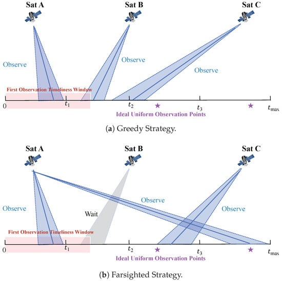
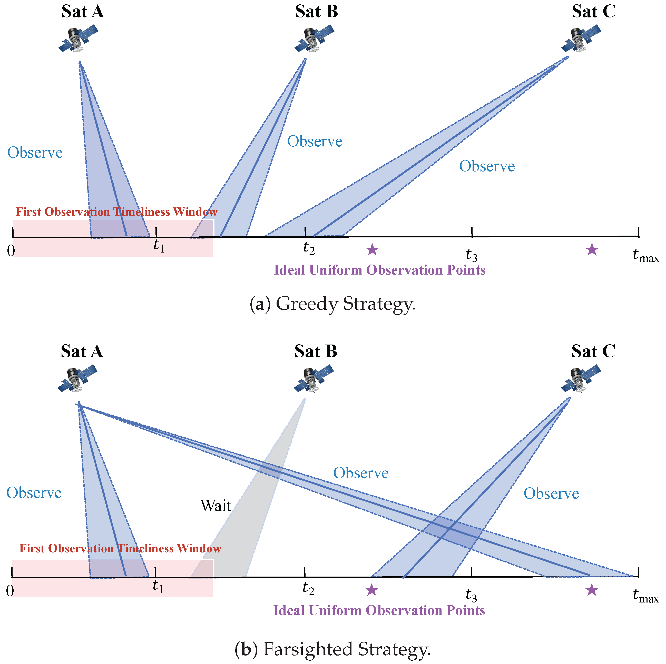
As illustrated in Figure 1, a simplified scenario reveals the core conflict in our scheduling problem. The figure depicts a scheduler coordinating Satellites A, B, and C to perform three observations for a single task. The scheduler must navigate a fundamental trade-off between two objectives: first, meeting a strict timeliness constraint by performing the initial observation within the First Observation Timeliness Window; and second, achieving observation uniformity by aligning subsequent observations with the ideal uniform observation points.

Figure 1. An illustration of Multi Earth Observation Satellite Multi-Target Task Scheduling Problem.

The difference between a myopic and a strategic policy is clearly highlighted. The greedy strategy in Figure 1a secures observations from all satellites as early as possible, satisfying timeliness but resulting in a concentrated distribution. In contrast, the farsighted strategy in Figure 1b demonstrates a crucial strategic sacrifice. After Satellite A secures the initial timely observation, Satellite B waits, forgoing immediate opportunities. This strategic delay allows subsequent observations to align with ideal points that are dynamically calculated to create a uniform distribution over the remaining time horizon. Achieving this essential strategic balance, however, requires the scheduling framework to overcome two significant inherent complexities.

Firstly, it is highly challenging to maintain temporally uniform observation intervals for all tasks across the entire scheduling horizon. Since tasks are released in specific geographic regions accessible only to a subset of satellites, and the optimal observation intervals for each task are dynamically determined only after its initial capture, selecting appropriate satellites to execute these subsequent observations becomes computationally intractable.

Secondly, modeling and capturing the dynamic balance among competing optimization objectives is highly challenging. For example, for a satellite to improve the revisiting uniformity, it may need to forgo some immediate observation opportunities, which could lead to a decrease in the total number of completed tasks. Consequently, intelligent decision-making must involve a complex trade-off. However, existing Deep Reinforcement Learning (DRL) methods often struggle to learn this specific dynamic balance. They typically rely on myopic state representations focused solely on immediate task availability, lacking the explicit temporal memory required to anticipate how current actions affect future revisit uniformity. Furthermore, the delayed nature of uniformity-related rewards makes it difficult for standard DRL agents to resist the temptation of immediate task completions, frequently resulting in degenerate policies that heavily favor one objective over the other.

The MSOTS framework provides a novel that is a direct response to the limitations of existing DRL methods, specifically addressing the dynamic balance required for multi-objective trade-offs. Rather than merely applying a standard MARL algorithm, MSOTS introduces a spatiotemporal-aware feature engineering mechanism. By embedding past observation histories and global resource scarcity indicators into the agents’ local states, it shifts the scheduling paradigm from reactive execution to proactive planning. Furthermore, to rigorously evaluate whether this complex trade-off is genuinely achieved, we introduce a Composite Multi-Objective Performance Score ($S_{\mathrm{MOP}}$). Unlike conventional linear metrics that can mask severe performance imbalances, $S_{\mathrm{MOP}}$ utilizes a weighted harmonic mean to strictly penalize degenerate scheduling behaviors, providing a more accurate and practical assessment of the learned policies. The primary contributions of this work are summarized as follows:

• The MSOTS framework leverages the power of MARL, enabling satellites to not only ensure coherent team-level strategies but also exhibit inherent scalability and strong generalization capabilities, allowing policies trained on a given scale to be directly deployed in significantly larger and more complex scenarios.
• To address the critical challenge of balancing task timeliness with uniform revisit intervals, we introduce a novel guidance mechanism. This mechanism leverages sophisticated feature engineering to prioritize the temporal distribution of observations while strictly adhering to first-observation deadlines.
• By leveraging the Multi-Agent Proximal Policy Optimization (MAPPO) algorithm, the framework enables agents to develop a sophisticated scheduling policy that dynamically seeks near-optimal solutions.
• The effectiveness and superiority of the method are validated through extensive simulations on large-scale datasets, demonstrating its robust performance in solving complex satellite task scheduling problems.

The remainder of this paper is organized as follows. Section 2 reviews the related work on satellite observation scheduling and MARL. Section 3 provides a formal description of the multi-satellite multi-target observation task scheduling problem, detailing the task request models, orbital mechanics constraints (including visibility windows and payload cooling time), and the optimization objectives. Section 4 presents the proposed MSOTS framework, formulating the scheduling problem as a Markov game. This section details the core components of the framework, including the MAPPO-based architecture under the CTDE paradigm, the construction of sophisticated spatiotemporal feature vectors for local observations and global states, and the design of an Operational Constraint Mask to ensure physical feasibility. Furthermore, it introduces the Composite Multi-Objective Performance Score based on a weighted harmonic mean to balance task completion, timeliness, and revisit uniformity. Section 5 reports the experimental results, providing a comprehensive analysis of the framework’s performance through baseline comparisons and ablation studies. Finally, Section 6 concludes the paper and outlines directions for future work.

2. Related Work

This section reviews literature on satellite task scheduling, covering both traditional algorithms and recent advancements in Deep Reinforcement Learning (DRL).

2.1. Traditional Satellite Task Scheduling Methods

Traditional methods for satellite task scheduling, while foundational, face limitations in dynamic, large-scale scenarios. Rule-based methods [7] are simple but myopic, often leading to local optima by ignoring long-term objectives. Exact algorithms guarantee optimality, but at a high computational cost. For instance, Chu et al. [8] proposed an Anytime Branch-and-Bound algorithm to address dynamic task scheduling, and Kim et al. [9] formulated the heterogeneous satellite scheduling problem as an MILP model. Despite their ability to find optimal solutions, the exponential complexity and static nature of these methods render them impractical for real-time applications. Heuristic and metaheuristic approaches, such as genetic algorithms [10] or hybrid neural network methods [11,12], offer more practical solutions but often require extensive problem-specific engineering and struggle to adapt to dynamic operational changes [13].

2.2. Deep Reinforcement Learning for Satellite Task Scheduling

The advancement of Artificial Intelligence has spurred the application of DRL, a promising model-free approach, to satellite scheduling [14,15]. The success of DRL in solving large-scale sequential decision-making problems, exemplified by AlphaGo’s breakthrough in the game of Go [16], has encouraged its use in this complex domain. Initial research focused on adapting fundamental DRL algorithms. For instance, He et al. [17] trained a Q-network to evaluate task sequences, while Huang et al. [18] employed the DDPG algorithm for continuous-time scheduling. As the field evolved, research focus significantly shifted toward multi-agent systems. Li et al. [19] proposed a method based on Multi-Agent DDPG (MADDPG) for autonomous collaboration, and more recently, Zhang et al. [20] utilized the MAPPO algorithm. Furthermore, advanced architectures have been explored to enhance performance. Wang et al. [21] proposed an encoder-decoder architecture for periodic tasks, Li et al. [22] designed a framework using an attention mechanism to improve scalability, and Chen et al. [23] introduced a hybrid method that combines DRL with rule-based heuristics.

Although these DRL approaches have shown significant promise, a notable gap remains. They often lack sophisticated mechanisms to explicitly handle the complex multi-objective trade-offs inherent in modern satellite tasks. The objective of maximizing task completion often conflicts with ensuring timeliness and achieving a uniform distribution of revisit observations for data continuity. A greedy approach to maximizing completion rates can compromise data quality, while waiting for an optimal revisit window may violate strict timeliness deadlines. Our work directly addresses this gap by designing a novel multi-agent reinforcement learning framework with a custom-designed reward function. This framework incentivizes task completion while carefully balancing on-time first observations and temporally uniform subsequent revisits.

3. Problem Formulation

This section provides a formal mathematical description of the multi-satellite cooperative task scheduling problem.

Given a system consisting of N satellites and a set of M observation tasks, we denote the set of satellites as $\mathcal{S}=\{{\mathrm{sat}}_1,{\mathrm{sat}}_2,\dots ,{\mathrm{sat}}_N\}$ and the set of tasks as $\mathcal{T}=\{{\mathrm{task}}_1,{\mathrm{task}}_2,\dots ,{\mathrm{task}}_M\}$. Furthermore, the scheduling horizon is discretized into a finite sequence of time steps, represented by the set $\mathcal{H}=\left\{0,1,\dots ,t_{max}\right\}$, where each index $t\in \mathcal{H}$ corresponds to a discrete decision point. Each task $i\in \mathcal{T}$ is defined by its own attributes, including a priority $P_i$, a required payload type ${load}_i$, an observation duration ${Dur}_i$, and a required number of revisits $C_i$. The scheduling opportunities are constrained by the set of visible time windows $\left(T{W}_{i,j}\right)$, which represent subsets of the scheduling horizon $\mathcal{H}$ during which a task is visible to a satellite. Correspondingly, each satellite $j\in \mathcal{S}$ possesses its own capabilities, including a specific equipped payload type, denoted as $LOA{D}_j$.

A core binary decision variable is defined as follows:

$$x_{i,j}\left(t\right)\in \{0,1\},\forall i\in \mathcal{T},\forall j\in \mathcal{S},\forall t\in \mathcal{H}$$

(1)

where $x_{i,j}\left(t\right)=1$ if satellite j decides to start an observation activity for task i at the discrete time step t, and $x_{i,j}\left(t\right)=0$ otherwise. This variable directly models the sequential decision-making process carried out by each agent at every step of the scheduling horizon. A complete list and detailed definitions of all parameters and decision variables used throughout this paper are provided in Table 1.

Table 1. Symbols for the problem formulation.

Symbol	Description
$\mathcal{S}$	Set of satellites, N in total
$\mathcal{T}$	Set of tasks, M in total
$\mathcal{H}$	Set of discrete time steps, $\mathcal{H}=\left\{0,1,\dots ,t_{max}\right\}$
$N,M$	Total number of satellites and tasks, respectively
$i,j$	Indices for tasks and satellites, respectively
t	A discrete time step in the scheduling horizon $\mathcal{H}$
$t_{max}$	The final time step in the scheduling horizon
$P_i$	Priority of task i
${\mathrm{load}}_i$	Required payload type for task i
${\mathrm{Dur}}_i$	Observation duration required for task i
$C_i$	Required number of revisits for task i
$T{W}_{i,j}$	Set of visible time windows between task i and satellite j
$LOA{D}_j$	Payload type equipped on satellite j
$x_{i,j}\left(t\right)$	Binary variable
$S_{\mathrm{comp}}$	Objective score for Task Completion
$S_{\mathrm{unif}}$	Objective score for Observation Uniformity
$S_{\mathrm{time}}$	Objective score for Task Timeliness
$w_c,w_u,w_t$	Weighting coefficients for the objectives
$S_{\mathrm{MOP}}$	The overall Multi-Objective Performance Score

The problem is formulated as a multi-objective optimization problem that seeks to simultaneously maximize the following three objectives.

• Task Completion ($S_{\mathrm{comp}}$): This objective quantifies the collective value derived from all successfully executed observations. It is calculated as the sum of priorities $P_i$ for each observation activity.

  $$S_{\mathrm{comp}}=\sum _{i=1}^M\sum _{j=1}^N\sum _{t=0}^{t_{max}}{P}_i·x_{i,j}\left(t\right)$$

  (2)
• Observation Uniformity ($S_{\mathrm{unif}}$): This objective evaluates the temporal uniformity of observation sequences, which is particularly critical for multi-revisit tasks. It incentivizes observation schedules where the intervals between consecutive observations are as evenly distributed as possible, a principle that is quantitatively defined in Section 4.4, as this often corresponds to higher-quality mission outcomes.
• Task Timeliness ($S_{\mathrm{time}}$): This objective evaluates the system’s rapid response to tasks. This metric is assessed solely by the time of a task’s first successful observation, independent of the total number of observations required. Timeliness is assessed based on a predefined deadline relative to a task’s earliest viable observation time. A detailed formulation of the timeliness score can be found in Section 4.4.

The multi-objective nature of the satellite task scheduling problem necessitates a comprehensive evaluation metric beyond a single measure such as total completed tasks. A high-performing method must strike a delicate balance between maximizing task completion, ensuring tasks are observed in a timely manner, and maintaining the temporal uniformity of observation intervals for revisit tasks.

To address this challenge, we introduce a composite evaluation metric predicated on a weighted harmonic mean. The decision to employ a harmonic mean, as opposed to a conventional arithmetic mean, is a deliberate modeling choice. In multi-objective scheduling, an arithmetic formulation is susceptible to the compensation effect, wherein disproportionately high performance in one objective (e.g., task completion) can mask critically deficient performance in another (e.g., revisit uniformity). By contrast, the harmonic mean inherently imposes a strong penalty on any low-performing objective. Leveraging this strict penalization is an intentional design principle—conceptually analogous to the F1-score—which ensures that a high overall score strictly necessitates a genuinely balanced and comprehensively effective scheduling strategy.

A critical consideration is that the individual objectives, $S_{\mathrm{comp}}$, $S_{\mathrm{unif}}$, and $S_{\mathrm{time}}$, operate on entirely different physical scales. To create a fair and balanced composite metric, we apply a Min-Max normalization process to scale all objectives into a common range of $[0,1]$. Since $S_{\mathrm{unif}}$ and $S_{\mathrm{time}}$ are inherently defined as ratios within $[0,1]$, they require no further transformation. For the completion score $S_{\mathrm{comp}}$, its theoretical minimum is 0, and its theoretical maximum is the sum of all task priorities. Therefore, its normalized form, $S_{\mathrm{comp},\mathrm{norm}}$, is strictly defined as:

$$S_{\mathrm{comp},\mathrm{norm}}={\displaystyle \frac{S_{\mathrm{comp}}}{{\sum }_{i=1}^M{P}_i}}$$

(3)

The overall objective is to maximize the Multi-Objective Performance Score ($S_{\mathrm{MOP}}$), which aggregates the weighted inverse of each normalized score. The score is defined as:

$$\mathrm{Maximize}{S}_{\mathrm{MOP}}={\displaystyle \frac{w_c+w_u+w_t}{I_{\mathrm{comp}}+I_{\mathrm{unif}}+I_{\mathrm{time}}}}$$

(4)

where $w_c,w_u,w_t$ are positive weighting coefficients, and the inverse scores $I_i$ are given by:

$$\begin{array}{cccccc}\hfill I_{\mathrm{comp}}& ={\displaystyle \frac{w_c}{S_{\mathrm{comp},\mathrm{norm}}}}\hfill & \hfill I_{\mathrm{unif}}& ={\displaystyle \frac{w_u}{S_{\mathrm{unif}}}}\hfill & \hfill I_{\mathrm{time}}& ={\displaystyle \frac{w_t}{S_{\mathrm{time}}}}\hfill \end{array}$$

By defining the problem as the maximization of this composite score, the model is able to learn and optimize all key dimensions of performance within a unified framework.

The model simplifies the complexity inherent in the satellite scheduling problem through several reasonable assumptions. Specifically, to ensure observational continuity, all tasks are assumed to be non-preemptive, requiring complete execution within an uninterrupted time period. Furthermore, a successful observation is contingent upon the imaging type matching between the task’s requirements and the satellite’s capabilities.

Based on these premises, the model is subject to the following hard constraints, which must be satisfied by any feasible solution.

$$t\notin T{W}_{i,j}\Rightarrow x_{i,j}\left(t\right)=0,\forall i\in \mathcal{T},\forall j\in \mathcal{S},\forall t\in \mathcal{H}$$

(5)

$$(loa{d}_i-LOA{D}_j)·x_{i,j}\left(t\right)=0,\forall i\in \mathcal{T},\forall j\in \mathcal{S},\forall t\in \mathcal{H}$$

(6)

$$\sum _{i=1}^M{x}_{i,j}\left(t\right)\le 1,\forall j\in \mathcal{S},\forall t\in \mathcal{H}$$

(7)

$$\sum _{j=1}^N{x}_{i,j}\left(t\right)\le 1,\forall i\in \mathcal{T},\forall t\in \mathcal{H}$$

(8)

Constraint (5), the time window constraint, ensures that the execution interval for any task i falls completely within the available visibility window of the observing satellite. Constraint (6), the payload type constraint, dictates that a task can only be assigned to a satellite equipped with a compatible payload type. Constraint (7), the single-task execution constraint, enforces that a satellite cannot perform multiple tasks simultaneously by preventing any temporal overlap between their execution windows. Constraint (8), the observation activity exclusivity constraint, ensures that a task can only be observed by one satellite at any given moment. Finally, in addition to the mathematical constraints, a minimum time gap between two consecutive observation activities on the same satellite is mandated.

To intuitively illustrate these constraints, consider a simplified scenario involving Satellite j (equipped with an optical sensor) and Task i (requiring a Synthetic Aperture Radar, SAR). Constraint (6) immediately masks any action for Satellite j to observe Task i due to payload incompatibility. Suppose instead Task i requires an optical sensor, satisfying Constraint (6). If the current time t falls outside the visible time window $T{W}_{i,j}$, Constraint (5) ensures the observation cannot occur. Furthermore, if Satellite j is already executing another task at time t, Constraint (7) prevents it from simultaneously observing Task i. Conversely, if another satellite is already observing Task i at time t, Constraint (8) guarantees that Satellite j will not duplicate the effort at the exact same moment, ensuring resource efficiency.

4. Methodology

Multi-satellite cooperative mission scheduling is fundamentally a multi-agent sequential decision-making process. We model this process as a Markov Game, an extension of the Markov Decision Process (MDP) to a multi-agent setting [24].

4.1. Multi-Agent Reinforcement Learning Setting

Essentially, multi-satellite collaborative task scheduling is a complex, large-scale optimization problem wherein multiple satellites must allocate resources and sequence their actions within a dynamic environment. The Markov Game provides a formal framework for this multi-agent sequential decision-making. The game is defined by a tuple $⟨N,S,\mathcal{A},R,P⟩$, where N is the set of satellite agents, S is the state space, $\mathcal{A}$ is the joint action space, R is the joint reward function, and P is the state transition probability function. The objective is to find a collective policy that optimizes the scheduling performance. The components are defined as follows.

(1)

State: The state provides the informational basis for the agents’ decision-making. To enable effective coordination, the state incorporates both global system information, which offers a macroscopic view of system progress and resource utilization, and each agent’s local observation, which contains the specific details needed for its individual decisions. The detailed feature engineering for the state representation is described in Section 4.3.

(2)

Action: The action space for each agent j at time step t, denoted as ${\mathcal{A}}_j\left(t\right)$, is a discrete set of available choices. At each decision point, an agent can select either to observe a specific task i or to execute No Operation (Wait). To manage the large action space, dynamic action filtering is employed, presenting each agent with only a subset of viable actions that satisfy all hard constraints.

(3)

Reward: To guide the agents toward the desired multi-objective outcome, a global reward function is shared by all agents. This reward is a scalar value computed at each time step, composed of several components designed to balance task completion, timeliness, and observation uniformity. The detailed formulation of the multi-objective reward function is presented in Section 4.4.

(4)

Transition: The state transition describes how the state of the system state evolves from the current time step t to the next, $t+1$, after the agents execute their actions. The state transition is deterministic and reflects changes in both agent and task status. For example, when an agent decides to execute a task, the task’s completion count increases. The state of the task is updated to reflect that its completed observation count has increased by one. If this count reaches the required number of observations $C_i$, the task is marked as completed.

4.2. Model Architecture

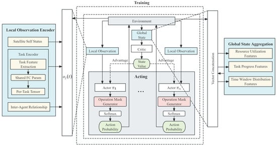
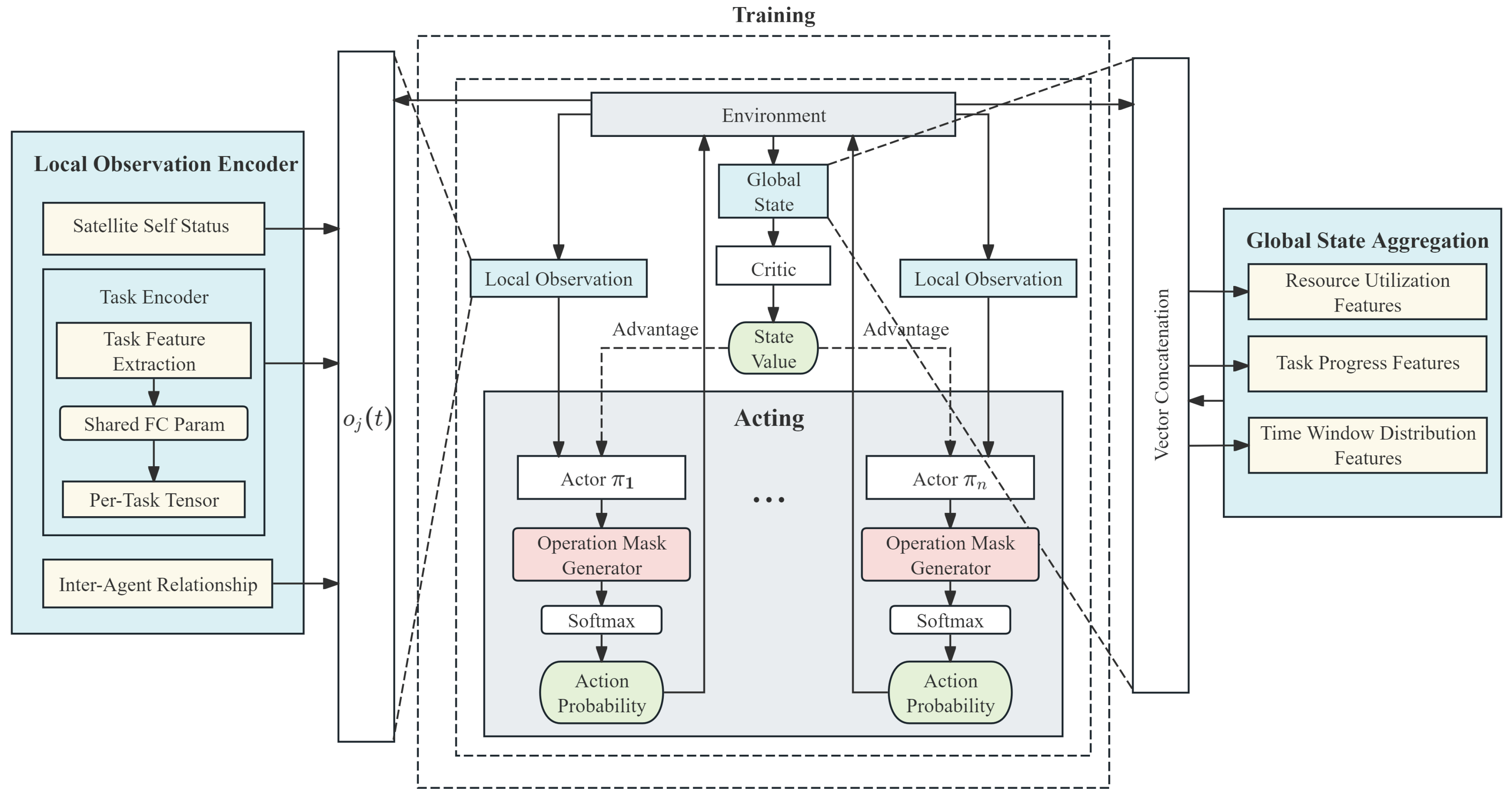
The proposed approach is based on a MARL framework, specifically adopting the CTDE paradigm. This design allows the model to leverage a global view of the environment during training, while enabling each satellite agent to make decisions independently during deployment. As shown in Figure 2, the system consists of a centralized Critic network and a single, shared Actor network.

Figure 2. Architecture of the MSOTS scheduling network.

In the training phase, the Critic network is a centralized component that evaluates the quality of the overall system state. The Critic has access to a global state aggregation module, which provides a comprehensive view of the entire scheduling problem by categorizing system-wide information into task progress, resource utilization, and time window distribution features. The Critic network comprises two fully connected layers (FC1, FC2) and outputs a single state value, which serves as a measure of the expected total reward from the current global state. The Actor network receives local observations from each agent and outputs an action probability distribution. The Critic’s state value is used to compute the Advantage for each action taken by the Actors, which is a key component for training the network.

For execution, the system operates in a decentralized manner. Although all agents share the same Actor network, each satellite agent only needs its local observation to make decisions. The Actor network takes a composite local observation vector $o_j\left(t\right)$ as input, which includes concatenated satellite, task, and inter-agent relationship features. Here, the task encoder plays a pivotal role. The raw observation vector is inherently complex, high-dimensional, and contains heterogeneous data (e.g., priorities, timestamps, status flags). Most importantly, it is of variable length because the number of tasks visible to a satellite changes at each time step. A standard neural network cannot directly process such dynamic-sized inputs.

To address this challenge, the raw task data is first processed by a dedicated task encoder. This encoder performs task feature extraction to parse the heterogeneous information. Its primary function is to take the variable-length task inputs and process them through shared fully connected layers to generate a per-task tensor, compressing the data into a fixed-size, dense latent representation. Fundamentally, it learns to extract the most critical information from all available tasks. This encoded task tensor, which now has a consistent structure regardless of the number of currently observable tasks, is then concatenated with the satellite self status and inter-agent relationship to form the final composite observation vector. This vector is then passed through the main Actor network. The subsequent network architecture, consisting of two fully connected layers (FC1, FC2), incorporates an operation mask generator to filter out invalid actions based on real-time constraints. Finally, a Softmax activation uses this rich, summarized information to output an action probability distribution over all available tasks. The agents do not require real-time communication with a central Critic or other agents to perform their tasks, allowing for efficient and robust operation. The parameters of the network are shown in Table 2 and Table 3.

Table 2. Actor network parameters.

Layer	Cells	Activation Function
Task Encoder	128	ReLU, LayerNorm
FC1	128	ReLU
FC2	128	ReLU
Output	number of tasks + 1	Softmax

Table 3. Critic network parameters.

Layer	Cells	Activation Function
FC1	128	ReLU
FC2	128	ReLU
Output	1	Identity

4.3. State Space Formulation

A carefully engineered state space is fundamental for enabling agents to perceive the environment and make informed decisions that balance conflicting objectives. For this purpose, a comprehensive state representation is designed, comprising both local observations for individual agents and a global state descriptor for the entire system.

Each agent’s local observation, denoted as $o_j\left(t\right)$, is a feature vector that provides all the necessary information for a local decision. Specifically, this includes a vector of features for each task that is valid for satellite j at time t. These task features are composed of three main categories: (1) task attributes, such as normalized priority $P_i$ and the remaining observation count $C_i-c_i\left(t\right)$, where $c_i\left(t\right)$ represents the number of observations already completed for task i up to time step t, (2) temporal features that capture task urgency, such as the time difference from the task’s earliest start time and the time remaining to its deadline; and (3) visibility and history attributes, including binary vectors indicating available and past time windows as well as past observation timestamps, which help evaluate revisit uniformity. In addition, satellite-specific attributes are incorporated, such as the satellite’s cooling-down time $C{D}_j\left(t\right)$, current operational status, and workload level. A ratio feature describing the remaining visible windows for a task relative to the total remaining windows across all satellites is also introduced to capture inter-agent relationships, reflecting resource scarcity and the balance between observation demand and supply.

The formulation of these local features fundamentally diverges from standard MARL state representations. While traditional approaches predominantly rely on myopic indicators of immediate task availability and priority, the incorporation of past observation timestamps establishes an explicit temporal memory mechanism. This allows the agent to continuously quantify deviations from ideal revisit intervals, effectively transitioning the decision-making paradigm from reactive, short-term task execution to proactive, long-term uniformity planning. Furthermore, the ratio of remaining visible windows functions as an implicit multi-agent coordination signal. By encoding constellation-wide resource scarcity into the local state, it enables individual agents to infer the global balance of observation supply and demand, thereby facilitating cooperative yielding behaviors to maintain an optimal temporal distribution of tasks.

Alongside local observations, a set of global features $s\left(t\right)$ provides a macroscopic description of the entire scheduling system via the global state aggregation module. These features are formed by aggregating information from all satellites, summarizing three main aspects: (1) overall task progress, including the task completion rate, the rate of uncompleted tasks satisfying timeliness, and the rate of multi-revisit tasks meeting uniformity requirements; (2) satellite resource utilization, which tracks the proportion of idle, working, and cooling satellites along with a metric for workload balance; and (3) time window distribution, which monitors the overall availability of remaining time windows, their time coverage across the scheduling horizon, and their density.

4.4. Multi-Objective Reward Shaping

A multi-component shaped reward function is formulated to address the credit assignment and reward sparsity challenges inherent in MARL, providing dense, step-by-step feedback to guide the agents’ learning process. It is carefully designed to steer the policy towards solutions that will ultimately achieve high scores on the global evaluation metrics $S_{\mathrm{comp}}$, $S_{\mathrm{time}}$ and $S_{\mathrm{unif}}$ defined in Section 3. The total reward is a linear combination of the following components, weighted by a set of tunable hyperparameters. The detailed calculation is presented in Algorithm 1.

(1)

Task Completion Reward ($r_{\mathrm{comp}}$): When a satellite successfully completes the observation of a task, it receives a large positive reward. This reward is proportional to the task’s priority, incentivizing the system to complete high-value tasks.

(2)

Timeliness Reward ($r_{\mathrm{time}}$): This reward is designed to quantify the system’s rapid response to tasks. This metric is assessed solely by the time of a task’s first successful observation. A constant time threshold ${\Delta }_t$ is employed as a hyperparameter to define the task’s deadline. The deadline for task i, $t_{\mathrm{deadline},i}$, is defined based on its earliest viable observation time, $t_{\mathrm{start},i}$, which is the minimum start time across all visible time windows for that task. The deadline is calculated as $t_{\mathrm{start},i}$ plus the time threshold:

$$t_{\mathrm{deadline},i}=t_{\mathrm{start},i}+{\Delta }_t$$

(9)

The attainment of the timeliness objective is represented by a binary step function:

$$S_{\mathrm{time},i}=\left\{\begin{array}{cc}1,\hfill & \mathrm{if}{t}_{\mathrm{obs},i,1}\le t_{\mathrm{deadline},i}\hfill \\ 0,\hfill & \mathrm{otherwise}\hfill \end{array}\right.$$

(10)

where $t_{\mathrm{obs},i,1}$ is the time of the first observation for task i. The overall system-level timeliness score $S_{\mathrm{time}}$ is then calculated as the proportion of all tasks that successfully meet their timeliness requirement, defined as:

$$S_{\mathrm{time}}={\displaystyle \frac{1}{M}}\sum _{i=1}^M{S}_{\mathrm{time},i}$$

(11)

The timeliness reward ($r_{\mathrm{time}}$) is distributed as a continuous function to provide a more nuanced gradient signal. This reward value smoothly decreases as the first observation time deviates from the task’s earliest start time, encouraging the agents to respond promptly.

(3)

Uniformity Reward ($r_{\mathrm{unif}}$): This reward is applied to multi-revisit tasks to measure the temporal uniformity of their observation sequences. It incentivizes schedules where the intervals between consecutive observations are as evenly distributed as possible. This uniformity is quantified by measuring the deviation between the actual observation intervals and an ideal interval using the normalized Mean Squared Error (MSE) as the primary metric. Let $t_{\mathrm{obs},i,k}$ be the time of the k-th observation for task i. The ideal interval, ${\Delta }_{\mathrm{ideal},i}$, is calculated by dividing the total available scheduling time for the task by the number of required revisits. The overall system-level uniformity, $S_{\mathrm{unif}}$, is derived from the individual uniformity errors of each task. Specifically, ${\mathrm{UniMse}}_i$ represents the MSE for an individual multi-revisit task i. The aggregate uniformity error, UniMse (defined in Equation (13)), is calculated as the arithmetic mean of ${\mathrm{UniMse}}_i$ over the set of all tasks that require two or more observations, denoted as ${\mathcal{T}}_{\mathrm{multi}}$. For any task $i\in {\mathcal{T}}_{\mathrm{multi}}$ that is observed fewer than two times, a maximum penalty error of ${\mathrm{UniMse}}_i=1.0$ is assigned to penalize its failure to establish a uniform observation pattern. This modeling choice is driven by both mathematical necessity, as calculating an interval inherently requires at least two data points and practical mission requirements, where a single observation fails to provide continuous dynamic monitoring. We acknowledge that under heavy task loads, this assumption strongly penalizes partially completed tasks. However, this introduces a deliberate and beneficial bias. Instead of encouraging a greedy strategy where agents spread resources too thinly to observe many tasks only once, this maximum penalty forces the system to commit its limited resources to ensure high-quality, repeated, and uniform observations for a subset of tasks. The aggregate error is thus formally defined as:

$${\mathrm{UniMse}}_i={\displaystyle \frac{1}{C_i-1}}\sum _{k=1}^{C_i-1}{\left({\displaystyle \frac{(t_{\mathrm{obs},i,k+1}-t_{\mathrm{obs},i,k})-{\Delta }_{\mathrm{ideal},i}}{{\Delta }_{\mathrm{ideal},i}}}\right)}^2$$

(12)

$$\mathrm{UniMse}={\displaystyle \frac{1}{|{\mathcal{T}}_{\mathrm{multi}}|}}\sum _{i\in {\mathcal{T}}_{\mathrm{multi}}}{\mathrm{UniMse}}_i$$

(13)

Finally, the overall observation uniformity score, Sunif, is defined as the complement of this aggregate error, rewarding lower average deviation:

$$S_{\mathrm{unif}}=1-\mathrm{UniMse}$$

(14)

Based on this MSE metric, the reward ($r_{\mathrm{unif}}$) is designed to be inversely proportional to the calculated deviation, providing a continuous signal to minimize the MSE.

(4)

Observation Penalty ($p_{\mathrm{obs}}$): To discourage myopic, closely-spaced observations and promote temporal uniformity, a penalty is applied. This is implemented via a retrospective interval deviation mechanism: upon a revisit observation, a penalty is calculated based on the deviation between the actual and an ideal observation interval. The penalty’s magnitude is an exponential function of this deviation. To enable proactive decision-making, future time window availability is encoded into the agent’s state representation. This allows the agent to learn the correlation between its current state and potential future penalties, thereby incentivizing it to wait for more opportune moments.

Algorithm 1 Shaped Reward Calculation

1: function CalculateShapedReward(event) Require:  An event object containing the observation time $t_{\mathrm{obs}}$ and the associated task. The task must provide its ID i,  priority $P_i$, required revisits $C_i$, and other scheduling parameters (e.g., $t_{\mathrm{start},i}$, ${\Delta }_{\mathrm{ideal},i}$).  2:    Initialize:reward  3:    $r_{\mathrm{comp}}\leftarrow {\alpha }_{\mathrm{comp}}·P_i$  4:    $\mathrm{reward}+=r_{\mathrm{comp}}$  5:    if  event.type is FirstObservation then  6:          $t_{\mathrm{start},i}\leftarrow \mathrm{task.earliest}\_\mathrm{start}\_\mathrm{time}$  7:          ${\Delta }_{\mathrm{delay}}\leftarrow max(0,t_{\mathrm{obs}}-t_{\mathrm{start},i})$  8:          $r_{\mathrm{time}}\leftarrow {\alpha }_{\mathrm{time}}·exp(-{\beta }_{\mathrm{time}}·{\Delta }_{\mathrm{delay}})$  9:          $\mathrm{reward} +=r_{\mathrm{time}}$  10:    else if event.type is SubsequentObservation then  11:         $t_{\mathrm{prev}\_\mathrm{obs},i}\leftarrow \mathrm{task.earliest}\_\mathrm{previous}\_\mathrm{observation}\_\mathrm{time}$  12:         ${\Delta }_{\mathrm{ideal},i}\leftarrow \mathrm{task.ideal}\_\mathrm{interval}$  13:         ${\Delta }_{\mathrm{actual}}\leftarrow t_{\mathrm{obs}}-t_{\mathrm{prev}\_\mathrm{obs},i}$  14:         ${\Delta }_{\mathrm{deviation}}\leftarrow |{\Delta }_{\mathrm{actual}}-{\Delta }_{\mathrm{ideal},i}|$  15:         $r_{\mathrm{unif}}\leftarrow {\alpha }_{\mathrm{unif}}·exp(-{\beta }_{\mathrm{unif}}·{\Delta }_{\mathrm{deviation}})$  16:         $p_{\mathrm{obs}}\leftarrow -{\alpha }_{\mathrm{penalty}}·exp({\beta }_{\mathrm{penalty}}·{\Delta }_{\mathrm{deviation}})$  17:         $\mathrm{reward} +=r_{\mathrm{unif}}+p_{\mathrm{obs}}$  18:     end if  19:     return reward  20: end function

4.5. Training Process

The entire framework is trained using the MAPPO algorithm, which is an on-policy method that collects complete experience trajectories during agent-environment interactions. The training is an iterative loop involving continuous interaction among the agents, the environment, and the Actor and Critic networks.

The process begins with an interaction between the agents and the environment. At each time step t, every satellite agent receives its local observation ($o_j\left(t\right)$), and uses a single, shared Actor network (${\pi }_{\varphi }$) to select an action. The joint action $a_t=\{a_{1,t},\dots ,a_{N,t}\}$ is executed, which leads to a new global state $s_{t+1}$ and a joint reward ${\mathbf{r}}_t$. This data is stored in a buffer to be used for gradient updates.

Simultaneously, a centralized Critic network ($\psi$) evaluates the global state($s\left(t\right)$) to predict a state value, $V_{\psi }\left(s\left(t\right)\right)$. This value is then used to compute the Generalized Advantage Estimation (GAE), ${\widehat{A}}_t$, which quantifies the advantage of the selected action relative to the expected policy performance, thereby guiding the actor’s policy updates. This advantage estimate provides a vital signal to guide the Actor’s policy updates.

Upon the completion of a trajectory, the network parameters are updated by minimizing specific loss functions. The Actor is updated using the PPO clipped surrogate objective [25], which ensures stable policy improvement by limiting the policy change in each update step. This is defined as:

$$L^{\mathrm{CLIP}}\left(\varphi \right)=\underset{t}{\mathbb{E}}\left[min\left(r_t\left(\varphi \right){\widehat{A}}_t,\mathrm{clip}(r_t\left(\varphi \right),1-ϵ,1+ϵ){\widehat{A}}_t\right)\right]$$

(15)

where $r_t\left(\varphi \right)={\displaystyle \frac{{\pi }_{\varphi }\left(a_t\right|o_j\left(t\right)}{{\pi }_{{\varphi }_{\mathrm{old}}}\left(a_t\right|o_j\left(t\right))}}$ is the probability ratio, and $ϵ$ is the clipping hyperparameter.

Concurrently, the Critic is trained to minimize the MSE between its predicted State Value and the calculated target returns, as shown in the following equation:

$$L_{\mathrm{value}}\left(\psi \right)=\underset{t}{\mathbb{E}}\left[{(V_{\psi }\left(s\left(t\right)\right)-R_t^{\mathrm{target}})}^2\right]$$

(16)

where $R_t^{\mathrm{target}}$ is the calculated target return.

Finally, to encourage exploration and prevent the policy from prematurely converging to a suboptimal solution, the total loss incorporates an entropy regularization term, S. The entropy loss, $L_{\mathrm{entropy}}\left(\varphi \right)$, is defined as the expected entropy of the policy distributions across all agents:

$$L_{\mathrm{entropy}}\left(\varphi \right)=\mathbb{E}\left[\sum _{i=1}^{N}S\left[{\pi }_{\varphi }(·|o_{j,t})\right]\right]$$

(17)

The final training objective is to minimize the following total loss, which combines all three components:

$$L_{\mathrm{total}}=L^{\mathrm{CLIP}}\left(\varphi \right)+c_1{L}_{\mathrm{value}}\left(\psi \right)-c_2{L}_{\mathrm{entropy}}\left(\varphi \right)$$

(18)

where $c_1$ and $c_2$ are the scaling coefficients for the value function loss and the entropy loss, respectively.

This iterative process allows the agents to learn an optimal scheduling policy over time. The overall training procedure is summarized in Algorithm 2.

Algorithm 2 The MSOTS Training Procedure based on MAPPO

Require:  Shared Actor Network ${\pi }_{\varphi }$, Shared Critic Network $V_{\psi }$.  Environment Env, A set of satellites $\mathcal{S}$, tasks $\mathcal{T}$,  Hyperparameters: Number of Episodes E; PPO Update Epochs K;  Number of training steps $\mathcal{H}$; Clip Ratio $ϵ$; GAE Parameter $\lambda$; Discount Factor $\gamma$. Ensure:  Trained network parameters: Actor ${\varphi }^{*}$ and Critic ${\psi }^{*}$. 1: Initialize: Actor network ${\pi }_{\varphi }$, Critic network $V_{\psi }$, their respective optimizers. 2: for each training episode $e=1$ to E do 3:     Reset environment Env, get initial state, and initialize trajectory buffer $\mathcal{D}$. 4:     for step $t=0$ to $\mathcal{H}$-1 do 5:       Construct state representation: 6:       for each agent $j=1,\dots ,N$ do 7:          $o_i\left(t\right)\leftarrow$ Construct local observation (incl. task, temporal, history, and inter-agent relation features.) 8:       end for 9:       $s\left(t\right)\leftarrow$ Construct global state (incl. system progress, resource utilization, and load balance). 10:     for each agent $i=1,\dots ,N$ do 11:        Sample action $a_i\left(t\right)\sim {\pi }_{\varphi }(·|o_i\left(t\right))$. 12:     end for 13:      Execute joint action $a_t$, environment returns next state $s_{t+1}$ and observation event event. 14:       ${\mathbf{r}}_t\leftarrow \mathrm{CalculateShapedReward}\left(\mathrm{event}\right)$ 15:       Store the complete transition in buffer $\mathcal{D}$. 16:     end for 17:     Compute advantages $\widehat{\mathbf{A}}$ using GAE and normalize them. 18:     for $k=1$ to K update epochs do 19:       for each mini-batch from $\mathcal{D}$ do 20:          From mini-batches, compute $L^{\mathrm{CLIP}}\left(\varphi \right)$, $L_{\mathrm{value}}\left(\psi \right)$, and 20:          $L_{\mathrm{entropy}}\left(\varphi \right)$. 21:          Calculate total loss $L_{\mathrm{total}}$. 22:          Perform backpropagation, gradient clipping, and Update 22:          network parameters $\varphi$ and $\psi$ via Adam optimizer 23:       end for 24:     end for 25: end for

4.6. Algorithm Complexity Analysis

This section aims to analyze the computational complexity of the MSOTS framework in both the training and execution phases to evaluate its feasibility for practical application.

4.6.1. Training Phase Complexity

The training phase is computationally intensive, but it is performed entirely offline. Its complexity is primarily influenced by several factors: the number of agents N, the number of tasks M, the number of timesteps per episode H, the number of PPO update epochs K, and the scale of the neural networks.

At each time step t, the system constructs local observations for N agents and the global state for the Critic. For each agent, the complexity of constructing its local observation is related to its number of visible tasks (at most M in the worst case). Subsequently, each agent performs a forward pass through the Actor network, with a complexity of $O\left(\mathrm{Size}\left(\mathrm{Actor}\right)\right)$. Concurrently, the Critic network processes the global state via a forward pass, with a complexity of $O\left(\mathrm{Size}\left(\mathrm{Critic}\right)\right)$. Therefore, the total complexity for collecting experience data within a single episode is approximately $O(H·N·\mathrm{Size}\left(\mathrm{Actor}\right)+H·\mathrm{Size}\left(\mathrm{Critic}\right))$.

During the parameter update stage, the algorithm utilizes the collected data to perform K epochs of optimization. The complexity of each epoch is proportional to the total volume of training data ($N\times H$) and the computational cost of backpropagation through the networks.

In summary, the training constitutes a process of polynomial-time complexity. Although computationally expensive, its one-time, offline nature renders it entirely acceptable prior to practical deployment.

4.6.2. Execution Phase Complexity

The low complexity of the execution phase is a core advantage of the MSOTS framework, highlighting its potential as a real-time decision-making solution.

During deployment and execution, the system is fully decentralized. At any given decision point, each satellite agent j independently performs the following operations:

1.

Acquire its local observation $o_j\left(t\right)$.

2.

Feed $o_j\left(t\right)$ into the pre-trained, shared Actor network for a single forward pass to obtain an action.

The computational complexity of a single decision is merely the cost of one forward pass through the Actor network, i.e., $O\left(\mathrm{Size}\left(\mathrm{Actor}\right)\right)$. Since the architecture of the Actor network is fixed and its size is independent of the number of agents N and tasks M, the decision-making time for a single agent is constant and highly efficient.

For the system as a whole, all N agents can make decisions in parallel at each decision step. The total computational load per step is therefore $O(N·\mathrm{Size}\left(\mathrm{Actor}\right))$, which scales linearly with the number of agents and ensures the system’s real-time feasibility.

5. Experiments and Evaluation

This section is dedicated to validating the performance of the proposed MSOTS framework. It outlines the experimental setup, provides a detailed description of the data used in the simulations, and presents a plan for comparative analysis against several algorithms.

5.1. Experimental Setup

To validate the MSOTS framework, a simulation environment was designed that reflects a realistic satellite scheduling scenario. The framework was implemented in Python 3.10.9 using the PyTorch 2.0.1 deep learning library. To ensure high physical fidelity, the Systems Tool Kit (STK) was employed to model the orbital dynamics of a large-scale Low Earth Orbit (LEO) constellation comprising 300 satellites. Specifically, the J2 perturbation model was adopted in STK to accurately account for the Earth’s oblateness and reflect real-world orbital mechanics. Furthermore, a dedicated scenario generator was implemented to randomly sample ground target positions within specific latitude and longitude ranges and compute the available observation windows for each satellite via STK. The specific parameters for the simulation environment and task configurations are detailed in Table 4.

Table 4. Simulation environment and parameter configuration.

Parameters	Values
Time Span	24 h
Total tasks Per Episode (M)	500
Total number of observations	1036
Number of Satellites (N)	300
Target Latitude Range	$-90$–${90}^{\circ }$
Target Longitude Range	$-180$–${180}^{\circ }$
Observation Duration ($Du{r}_i$)	20 s
Task Priority ($P_i$)	0–1
Number of revisits ($C_i$)	1–4
Constant time threshold (${\Delta }_t$)	3 h
Satellite Cooldown	20 s

The values of the hyper-parameters used in the experiments are shown in Table 5. A smaller discount factor ($\gamma$) is adopted in our approach, because our framework directly addresses long-term temporal dependencies by embedding temporal memory into the state space and employing a retrospective reward mechanism; utilizing a smaller $\gamma$ effectively truncates the compounding variance and credit assignment noise induced by dynamic multi-agent interactions. This design significantly stabilizes the training process without compromising the model’s capacity for farsighted planning.

Table 5. Hyper parameters for training.

Parameters	Values
Number of Episodes (E)	300
PPO Update Epochs (K)	2
Number of training steps ($\mathcal{H}$)	4320
Clip Ratio ($ϵ$)	0.15
GAE Parameter ($\lambda$)	0.95
Discount Factor ($\gamma$)	0.7
Reward loss coefficient ($c_1$)	0.5
Entropy coefficient ($c_2$)	0.03

The complete source code for the MSOTS framework, including the environment implementation and the MAPPO training procedure, has been made publicly available on GitHub to ensure reproducibility. The repository can be accessed at: https://github.com/maomao0324/MSOTS (accessed on 1 January 2026).

5.2. Compared Algorithms

To further validate the effectiveness of the proposed approach, a series of comparative experiments were conducted. The model was benchmarked against a wide range of baselines, from traditional scheduling algorithms to reinforcement learning algorithms. These experiments aim to demonstrate the framework’s superiority in managing the complex, multi-objective trade-offs inherent in satellite task scheduling. All comparison algorithms were evaluated using the same simulation environment and parameter configurations, ensuring a fair and consistent assessment.

• Greedy Algorithm At each decision step, this algorithm selects the task offering the highest immediate reward. Its objective is to maximize short-term gains, using the same reward function as the other baselines.
• Simulated Annealing (SA) Algorithm A metaheuristic algorithm that explores the solution space to find a near-optimal solution. Its objective is to maximize the same composite reward function used in the proposed MARL model. The specific hyperparameter configuration for the SA algorithm is detailed in Table 6. In the simulated annealing baseline, each candidate solution is encoded as a one-dimensional integer array that maps precomputed valid time steps to either specific task indices or an idle state. To explore the solution space, we employ a heuristic-guided mutation operator to generate neighboring states. This mechanism balances exploration and exploitation by probabilistically alternating among three distinct behaviors: adopting an idle state, prioritizing tasks that require multiple revisits, and randomly selecting alternative feasible tasks.
• MADDPG A distributed scheduling algorithm from [19] based on Multi-Agent DDPG. It enables autonomous satellite collaboration with low communication overhead by having agents share policies instead of state data.
• SRADA-DRL A method from [23] that first uses deep reinforcement learning (DRL) for mission allocation among satellites, then applies a rule-based heuristic to determine final start and end times. The goal is to maximize total profit while managing resource contention.
• ST-VP (Spatiotemporal Value-based Planning): An industrial-grade coordination framework adapted from [26] that decomposes the scheduling problem into two synergistic phases. The learning phase utilizes historical data to estimate the expected future value of agents in specific spatiotemporal states. The subsequent scheduling phase performs real-time combinatorial optimization to match agents with tasks, effectively balancing immediate observation rewards with future mission gains. This approach was originally developed for and successfully deployed in the large-scale production systems of DiDi Chuxing.

Table 6. Simulated Annealing (SA) parameter configuration.

Parameters	Values
Initial Temperature ($T_0$)	1000.0
Cooling Rate	0.95
Final Temperature ($T_{\mathrm{final}}$)	0.1
Iterations per Temperature Level	500

5.3. Analysis of Training Results

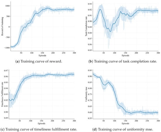
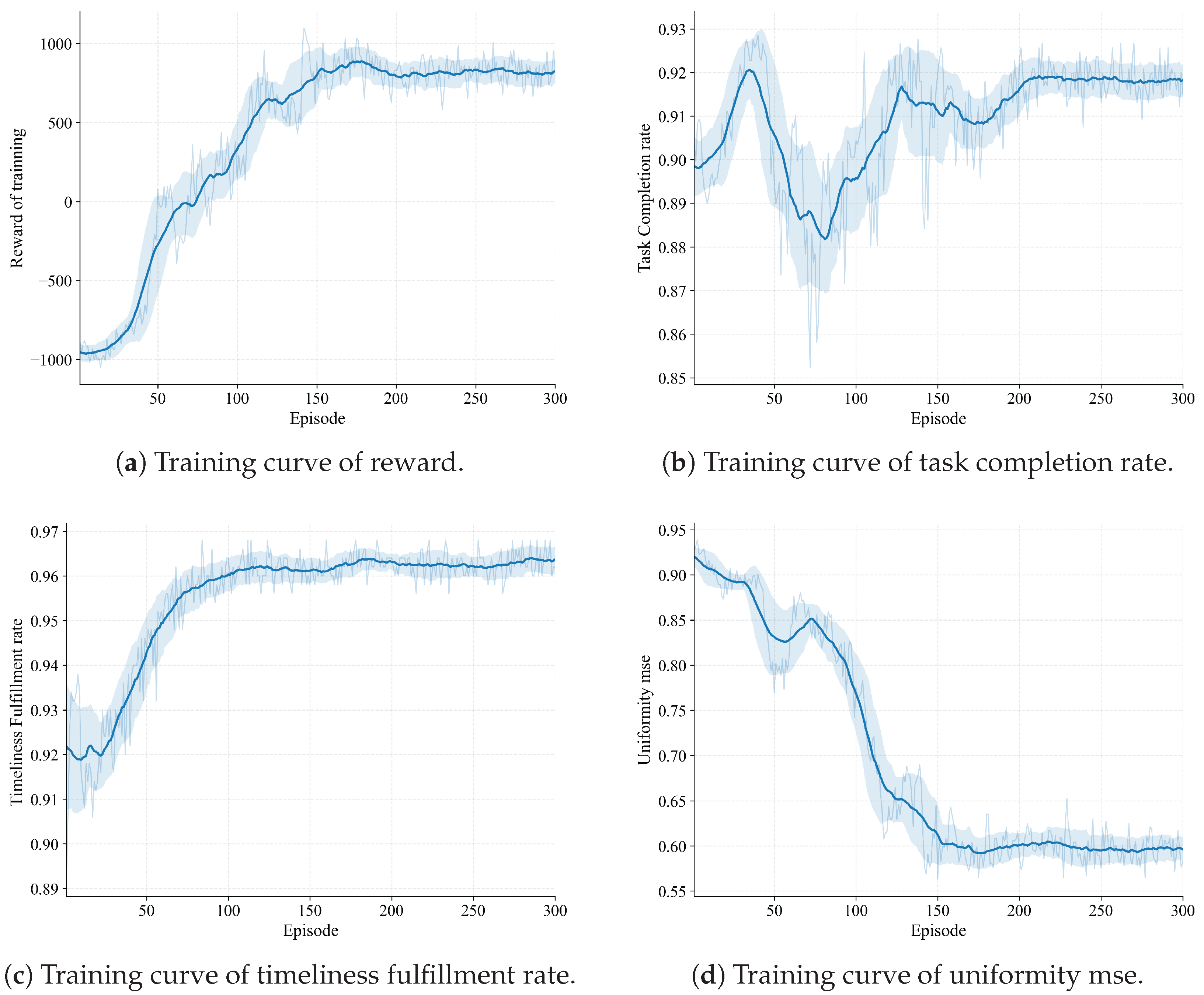
The training performance across four key metrics demonstrates a robust and convergent learning process.

As depicted in Figure 3a, the episodic reward rapidly ascends from negative values and converges to a stable plateau of approximately 850, indicating the acquisition of a near-optimal policy.

Figure 3. Training performance of the MSOTS framework. (a) reward (b) task completion (c) timeliness (d) uniformity mse.

Figure 3b illustrates the task completion rate, which, after some initial oscillations, stabilizes at a high level of approximately 92%, demonstrating the model’s ability to effectively complete a large volume of tasks.

The timeliness fulfillment rate, depicted in Figure 3c, shows the most rapid convergence, quickly exceeding and maintaining a stable rate above 96%, highlighting the model’s efficiency in handling time-sensitive requirements.

As detailed in Figure 3d, the uniformity MSE curve displays a distinct downward trend, decreasing from approximately 0.9 to a stable value of 0.6, confirming the model’s success in learning to schedule tasks with a uniform temporal distribution.

Collectively, this evidence confirms that the proposed framework is effective at solving the multi-objective satellite task scheduling problem by simultaneously optimizing for all four objectives.

5.4. Baseline Comparison Analysis

To validate the efficacy of the proposed MSOTS framework, extensive comparative experiments were conducted. All policies were rigorously benchmarked using the composite metric $S_{\mathrm{MOP}}$, as defined in Section III. For this analysis, the weighting coefficients were empirically set to $w_c=1.0$, $w_u=0.8$, and $w_t=0.8$. Rather than treating raw task completion as the sole overriding priority, this configuration reflects the evolving operational demands of modern Earth observation missions. It establishes a foundational baseline for mission yield ($w_c$) while placing substantial emphasis on data quality through temporal uniformity ($w_u$) and timeliness ($w_t$). This ensures the evaluation favors well-distributed and rapid responses over purely quantity-driven greedy scheduling, aligning with practical scenarios where timely and continuous monitoring is paramount.

The results, presented in Table 7 and Table 8, demonstrate the superiority of the MSOTS framework. In the 500-task scenario, MSOTS achieves the highest best-case $S_{\mathrm{MOP}}$ of 0.680, showcasing its ability to find a balanced solution. Furthermore, the statistical results evaluated across multiple random seeds ($0.567\pm 0.091$) confirm the algorithmic stability and robustness of MSOTS, consistently outperforming the baselines. In contrast, other algorithms exhibit clear trade-off failures. For instance, while SRADA-DRL and MADDPG achieve high completion rates of 95.1% and 91.89% respectively, they suffer from extremely poor uniformity, reflected in their respective $S_{\mathrm{unif}}$ scores of 0.066 and 0.0492. Consequently, their overall performance is severely compromised, yielding $S_{\mathrm{MOP}}$ values of merely 0.186 and 0.143. While the Greedy algorithm shows better uniformity with an $S_{\mathrm{unif}}$ of 0.385, its short-sighted strategy leads to a low completion rate of 63.6%, limiting its overall effectiveness.

Table 7. Performance comparison (300 satellites with 500 observation tasks).

Method	Completion (%)	${\mathit{S}}_{\mathbf{comp}}$	${\mathit{S}}_{\mathbf{time}}$	UniMse	${\mathit{S}}_{\mathbf{unif}}$	${\mathit{S}}_{\mathbf{MOP}}$
Greedy	63.60	166.24	0.988	0.6150	0.3850	0.505
SA	97.80	368.10	0.962	0.9830	0.0170	0.053
SRADA-DRL	95.10	354.48	0.970	0.9340	0.0660	0.186
ST-VP	93.80	354.00	0.960	0.9349	0.0651	0.183
MADDPG	91.89	344.81	0.910	0.9508	0.0492	0.143
MSOTS (Best)	92.60	338.71	0.968	0.5760	0.4240	0.680
MSOTS (Mean ± SD)	91.85 ± 0.69	339.85 ± 2.49	0.967 ± 0.002	0.6980 ± 0.084	0.3020 ± 0.084	0.567 ± 0.091

Table 8. Performance comparison (300 satellites with 800 observation tasks).

Method	Completion (%)	${\mathit{S}}_{\mathbf{comp}}$	${\mathit{S}}_{\mathbf{time}}$	UniMse	${\mathit{S}}_{\mathbf{unif}}$	${\mathit{S}}_{\mathbf{MOP}}$
Greedy	58.86	313.95	0.989	0.6250	0.3750	0.490
SA	94.75	732.95	0.997	0.9970	0.0030	0.010
SRADA-DRL	93.62	700.62	0.970	0.9461	0.0539	0.155
ST-VP	93.62	700.20	0.970	0.9472	0.0528	0.153
MADDPG	92.12	680.86	0.920	0.9466	0.0534	0.153
MSOTS (Best)	90.01	653.24	0.964	0.5231	0.4769	0.713
MSOTS (Mean ± SD)	90.85 ± 0.94	665.05 ± 11.06	0.970 ± 0.004	0.6680 ± 0.098	0.3320 ± 0.098	0.589 ± 0.085

To explicitly evaluate the scalability and generalization capabilities of the proposed framework across different task densities, we directly applied the MSOTS model—trained exclusively on the 500-task scenario—to a significantly denser 800-task scenario without any retraining or fine-tuning. The superiority of MSOTS becomes even more pronounced in this high-load environment, where its best $S_{\mathrm{MOP}}$ increases to 0.713. The average performance ($0.589\pm 0.085$) across multiple inference seeds further verifies that this is a consistently learned capability rather than an anomalous spike. This direct transferability highlights its excellent scalability and performance resilience against exponentially increased conflict rates. Under this increased pressure, the performance of methods like SA collapses, with its $S_{\mathrm{unif}}$ score dropping to just 0.003 and its $S_{\mathrm{MOP}}$ to 0.010. This severe degradation occurs because SA, inherently a static global optimization algorithm, struggles to adapt to the dynamic, step-by-step nature of our scheduling environment, where decisions must be made sequentially based on real-time observations of executable tasks. Furthermore, the DRL baselines struggle significantly to adapt; SRADA-DRL and MADDPG fail to balance the conflicting objectives under severe resource constraints, resulting in stagnant $S_{\mathrm{MOP}}$ scores of 0.155 and 0.153, respectively.

Collectively, these results confirm that MSOTS learns a robust, farsighted policy that successfully navigates complex multi-objective trade-offs across different load scenarios, a direct result of its specialized reward architecture and training paradigm. The policy empowers individual satellite agents to make globally optimal collaborative decisions, particularly concerning uniformity, in the absence of real-time centralized communication. Consequently, it dramatically surpasses baseline methods which are either myopic or fail to balance multiple conflicting objectives with respect to the $S_{\mathrm{MOP}}$.

5.5. Ablation Study

The ablation study in Table 9 confirms that the uniformity-aware reward function is decisive for achieving a high-quality, balanced solution.

Table 9. Ablation study (300 satellites with 500 observation tasks).

Method	Completion (%)	Scomp	Stime	UniMse	Sunif	SMOP
MSOTS ($r_{\mathrm{simple}}$)	94.50	350.57	0.96	0.9373	0.0627	0.1773
MSOTS (full)	92.6	338.71	0.968	0.576	0.424	0.680

The simplified MSOTS model, which omits the uniformity reward and observation penalty, degenerates into a myopic strategy. Although it achieves a marginally higher completion rate of 94.50%, it suffers a catastrophic degradation in uniformity, yielding an $S_{\mathrm{unif}}$ score of merely 0.0627. Consequently, its overall performance score, $S_{\mathrm{MOP}}$, plummets to 0.1773.

In stark contrast, our full MSOTS model accepts a minor 2% drop in completion rate to achieve a vastly superior uniformity score $S_{\mathrm{unif}}$ of 0.424. This balanced trade-off leads to a nearly fourfold increase in the comprehensive score, with an $S_{\mathrm{MOP}}$ of 0.680. This demonstrates that harmonizing multiple objectives is far superior to maximizing a single metric at the expense of others.

5.6. Sensitivity Analysis of Objective Weights

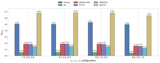
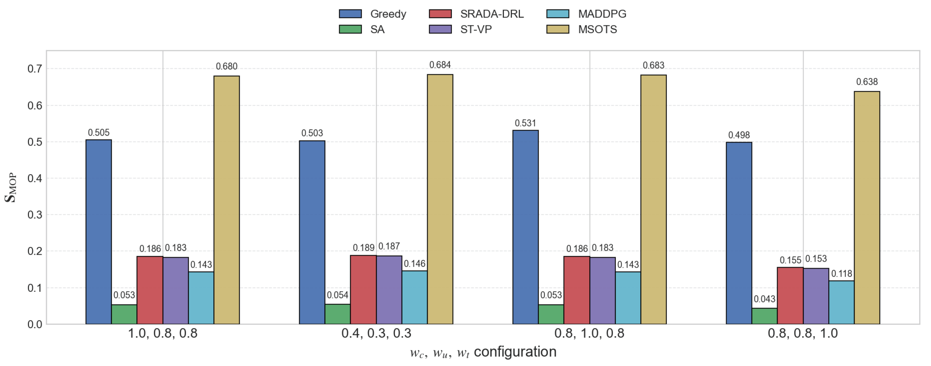
To evaluate the robustness and adaptability of the proposed MSOTS framework under varying mission priorities, a sensitivity analysis of the objective weights $(w_c,w_u,w_t)$ was conducted. Figure 4 illustrates the comprehensive performance metric $S_{MOP}$ across different weight configurations, which represent specific operational preferences such as task completion focus, uniformity focus, timeliness focus, and equal importance.

Figure 4. Sensitivity Analysis of $S_{MOP}$ under different weight configurations—500 tasks scenario.

As shown in the results, MSOTS consistently outperforms all baseline algorithms—including Greedy, SA, SRADA-DRL, MADDPG, and ST-VP—across all tested weight combinations. Notably, while the performance of traditional heuristic methods and other DRL baselines remains sub-optimal or fluctuates depending on the weight distribution, MSOTS maintains a highly stable and superior $S_{MOP}$ score (ranging from 0.638 to 0.684). This stability demonstrates that the spatiotemporal-aware multi-objective design of MSOTS is highly robust. It can effectively balance competing objectives and seamlessly adapt to diverse operational requirements without experiencing significant performance degradation. Consequently, MSOTS proves to be highly reliable for complex, real-world satellite scheduling scenarios where mission priorities may dynamically shift.

6. Discussion

This study introduces the MSOTS framework, a spatiotemporal-aware multi-agent reinforcement learning approach tailored for multi-satellite observation task scheduling with periodic revisit requirements. The experimental results demonstrate that MSOTS consistently outperforms traditional heuristic methods and existing deep reinforcement learning-based approaches across multiple evaluation dimensions. In this section, the results are discussed by integrating quantitative performance analysis with qualitative interpretation, focusing on multi-objective trade-offs, generalization capability, and the contribution of key design components.

Quantitative comparisons indicate that MSOTS achieves a substantial improvement in comprehensive scheduling performance under typical operational scenarios. In the scenario comprising 300 satellites and 500 observation tasks, MSOTS enhances the composite $S_{\mathrm{MOP}}$ metric by approximately 35% relative to the greedy baseline, and demonstrates a more than threefold performance gain over the strongest deep reinforcement learning baselines. Importantly, these gains are obtained while maintaining a competitive task completion rate, suggesting that the overall performance improvement does not rely on sacrificing primary mission objectives such as task coverage or first-observation timeliness.

A closer inspection of individual performance dimensions reveals that the advantage of MSOTS primarily stems from its ability to balance competing objectives rather than aggressively optimizing a single metric. Although several baseline methods achieve marginally higher completion or timeliness scores, they exhibit severe degradation in revisit uniformity, which significantly compromises the overall mission quality. In contrast, MSOTS explicitly incorporates revisit-related optimization as a critical but subordinate objective, improving observation regularity while preserving satisfactory completion and temporal performance. This behavior confirms that revisit optimization in MSOTS serves as a complementary enhancement to conventional scheduling objectives, rather than a dominant priority.

To explicitly clarify the trade-off mechanism driving this behavior, MSOTS occasionally sacrifices marginal task completions to prevent temporal clustering. Algorithms that strictly maximize completion rates often employ opportunistic strategies, rushing to fulfill a task’s required number of revisits as quickly as possible. While this rapidly completes the tasks, it clusters the observations together, inevitably creating massive temporal blind spots for that target later in the scheduling horizon. MSOTS, guided by its uniformity-aware reward and spatiotemporal state representation, learns to strategically delay observations to maintain ideal intervals. By holding back to ensure an even distribution, the system may occasionally forgo opportunities to accommodate additional low-priority tasks. However, in practical mission contexts such as disaster response, maritime vessel tracking, or persistent environmental monitoring—this balanced approach is highly preferable. Receiving continuous, evenly spaced intelligence for a set of targets is far more actionable than achieving a higher raw completion rate where data is collected sporadically followed by long, unmonitored gaps. Therefore, the slight reduction in completion rate is a deliberate and necessary compromise to ensure the generation of highly reliable monitoring schedules.

The generalization capability of MSOTS is further validated under higher task-load conditions. When the number of observation tasks increases from 500 to 800, most baseline methods experience noticeable performance degradation, with $S_{\mathrm{MOP}}$ values remaining low or declining. By contrast, MSOTS not only maintains stable performance but achieves an even higher $S_{\mathrm{MOP}}$ score, improving by approximately 45% compared with the greedy baseline and by more than fourfold relative to existing deep reinforcement learning methods. Notably, the $S_{\mathrm{MOP}}$ value of MSOTS increases from 0.680 to 0.713 under heavier task loads, demonstrating strong robustness and effective generalization to more congested scheduling environments.

The ablation study provides additional insight into the effectiveness of the proposed framework. When the revisit-aware reward structure is simplified, the overall scheduling performance deteriorates significantly, with the composite $S_{\mathrm{MOP}}$ score reduced to less than one quarter of that achieved by the full MSOTS model. Although the simplified variant attains a slightly higher task completion rate, its revisit uniformity degrades severely, leading to poor comprehensive performance. This result highlights that the revisit-aware reward design and spatiotemporal state modeling are essential components of MSOTS rather than auxiliary refinements, and that their integration is crucial for achieving balanced multi-objective optimization.

From a methodological perspective, the MAPPO-based centralized training and decentralized execution paradigm plays a key role in enabling these performance gains. The shared policy structure facilitates implicit cooperation among satellites without requiring explicit inter-agent communication during execution, while the task encoder and spatiotemporal state representation allow the framework to adapt to dynamically changing observation opportunities. Together, these design choices enable MSOTS to learn farsighted scheduling policies that remain effective across different task scales and operational conditions.

Overall, the discussion confirms that the superior performance of MSOTS arises from its ability to integrate revisit-aware optimization into a balanced multi-objective learning framework. The quantitative improvements, strong generalization performance, and ablation results collectively demonstrate the robustness and effectiveness of the proposed approach for complex multi-satellite observation task scheduling problems.

7. Conclusions

This study presents the MSOTS framework, a multi-agent reinforcement learning-based solution for complex multi-satellite observation task scheduling problems. By formulating the scheduling process as a Markov game and employing a custom-designed multi-objective reward function within the MAPPO algorithm, MSOTS effectively balances task completion, first-observation timeliness, and revisit-related optimization requirements. Extensive experimental results demonstrate that the proposed framework achieves superior comprehensive performance and stability compared with traditional heuristic methods and existing deep reinforcement learning baselines, particularly under high task-load conditions.

Despite these promising results, the current mathematical formulation relies on certain simplifying assumptions, such as non-preemptive tasks and fixed payload compatibility, which may limit its immediate applicability in highly complex real-world environments. Regarding scalability, introducing heterogeneous, multi-payload satellites would significantly expand the state and action spaces. To maintain training efficiency and scalability under such conditions, future models could incorporate attention-based payload-matching masks or hierarchical reinforcement learning architectures. Regarding extensibility, the MSOTS framework can be adapted to handle preemptive tasks by modifying the action space to allow task interruption and augmenting the state space to track partial completion rates. To prevent excessive task fragmentation, a preemption penalty could be introduced into the reward function. Similarly, dynamic or heterogeneous payloads can be accommodated by embedding real-time payload-task compatibility matrices into the agents’ local state representations. Incorporating these online learning or model-based reinforcement learning (MBRL) mechanisms, together with explicitly modeling uncertainty in satellite states (e.g., weather disturbances, sensor failures), represents a critical direction for our future work to enable rapid resource reallocation under abrupt operational changes.

Moreover, recent advances in space–air communication networks and on-orbit processing provide new opportunities for extending the proposed framework. For example, integrating network-aware mechanisms for anomaly detection and communication reliability [27] can enhance the robustness of data return following observation tasks. From a broader system perspective, MSOTS can also be viewed as a key component within emerging Orbital Edge Computing (OEC) architectures [28]. Co-designing task scheduling policies with OEC resource management strategies, as well as incorporating robust optimization or partially observable Markov decision process (POMDP) formulations, represents a promising direction for achieving more resilient and efficient satellite mission planning.

Overall, this work provides a solid foundation for intelligent, revisit-aware multi-satellite task scheduling and offers valuable insights for future research on learning-based space mission planning under complex and dynamic operational constraints.

References

- Huang, W.; Wang, H.; Wu, J.; Hou, H.; Li, J.; Li, Z.; Song, Y. A Reinforcement Learning-Enhanced Dung Beetle Optimization Approach for Agile Earth Observation Satellite Scheduling. IEEE Geosci. Remote Sens. Lett. 2025, 22, 8000305. [Google Scholar] [CrossRef] [Scilit]
- Tang, G.; Zeng, Z.; Ma, M.; Liu, R.; Wen, Y.; Hong, Y. Can near-real-time satellite precipitation products capture rainstorms and guide flood warning for the 2016 summer in South China? IEEE Geosci. Remote Sens. Lett. 2017, 14, 1208–1212. [Google Scholar] [CrossRef] [Scilit]
- Chang, S.; Wu, B.; Yan, N.; Zhu, J.; Wen, Q.; Xu, F. A refined crop drought monitoring method based on the Chinese GF-1 wide field view data. Sensors 2018, 18, 1297. [Google Scholar] [CrossRef] [Scilit] [PubMed]
- Ahmed, M.R.; Rahaman, K.R.; Kok, A.; Hassan, Q.K. Remote sensing-based quantification of the impact of flash flooding on the rice production: A case study over Northeastern Bangladesh. Sensors 2017, 17, 2347. [Google Scholar] [CrossRef] [Scilit]
- Irrgang, C.; Saynisch, J.; Thomas, M. Estimating global ocean heat content from tidal magnetic satellite observations. Sci. Rep. 2019, 9, 7893. [Google Scholar] [CrossRef] [Scilit]
- Wen, X.; Chen, B. A review of technical development of military reconnaissance satellite abroad. Mod. Def. Technol. 2001, 29, 5–8, 16. [Google Scholar]
- Liang, J.; Zhu, Y.h.; Luo, Y.z.; Zhang, J.c.; Zhu, H. A precedence-rule-based heuristic for satellite onboard activity planning. Acta Astronaut. 2021, 178, 757–772. [Google Scholar] [CrossRef] [Scilit]
- Chu, X.; Chen, Y.; Tan, Y. An anytime branch and bound algorithm for agile earth observation satellite onboard scheduling. Adv. Space Res. 2017, 60, 2077–2090. [Google Scholar] [CrossRef] [Scilit]
- Kim, C.H.; Kim, S.J.; Choi, H.L. Heterogeneous satellite task scheduling with revisit time minimization using milp formulation. In Proceedings of the AIAA SCITECH 2024 Forum, Orlando, FL, USA, 8–12 January 2024; p. 0747. [Google Scholar]
- Niu, X.; Tang, H.; Wu, L. Satellite scheduling of large areal tasks for rapid response to natural disaster using a multi-objective genetic algorithm. Int. J. Disaster Risk Reduct. 2018, 28, 813–825. [Google Scholar] [CrossRef] [Scilit]
- Chen, J.; Chen, M.; Wen, J.; He, L.; Liu, X. A heuristic construction neural network method for the time-dependent agile earth observation satellite scheduling problem. Mathematics 2022, 10, 3498. [Google Scholar] [CrossRef] [Scilit]
- Li, F.; Wan, Q.; Wen, F.; Zou, Y.; He, Q.; Li, D.; Zhong, X. Multi-Satellite Imaging Task Planning for Large Regional Coverage: A Heuristic Algorithm Based on Triple Grids Method. Remote Sens. 2024, 16, 194. [Google Scholar] [CrossRef] [Scilit]
- Wang, J.; Zhu, X.; Qiu, D.; Yang, L.T. Dynamic scheduling for emergency tasks on distributed imaging satellites with task merging. IEEE Trans. Parallel Distrib. Syst. 2013, 25, 2275–2285. [Google Scholar] [CrossRef] [Scilit]
- Jiang, R.; Deng, Y.; Chen, Y.; Luo, H.; An, B. Deep reinforcement learning for multi-objective game strategy selection. Comput. Oper. Res. 2024, 168, 106683. [Google Scholar] [CrossRef] [Scilit]
- Sutton, R.S.; McAllester, D.; Singh, S.; Mansour, Y. Policy gradient methods for reinforcement learning with function approximation. In Proceedings of the 13th International Conference on Neural Information Processing Systems (NIPS’99), Denver, CO, USA, 29 November–4 December 1999; pp. 1057–1063. [Google Scholar]
- Silver, D.; Schrittwieser, J.; Simonyan, K.; Antonoglou, I.; Huang, A.; Guez, A.; Hubert, T.; Baker, L.; Lai, M.; Bolton, A.; et al. Mastering the game of go without human knowledge. Nature 2017, 550, 354–359. [Google Scholar] [CrossRef] [Scilit]
- He, Y.; Xing, L.; Chen, Y.; Pedrycz, W.; Wang, L.; Wu, G. A generic Markov decision process model and reinforcement learning method for scheduling agile earth observation satellites. IEEE Trans. Syst. Man Cybern. Syst. 2020, 52, 1463–1474. [Google Scholar] [CrossRef] [Scilit]
- Huang, Y.; Mu, Z.; Wu, S.; Cui, B.; Duan, Y. Revising the observation satellite scheduling problem based on deep reinforcement learning. Remote Sens. 2021, 13, 2377. [Google Scholar] [CrossRef] [Scilit]
- Li, D.; Wang, H.; Yang, Z.; Gu, Y.; Shen, S. An online distributed satellite cooperative observation scheduling algorithm based on multiagent deep reinforcement learning. IEEE Geosci. Remote Sens. Lett. 2020, 18, 1901–1905. [Google Scholar]
- Zhang, G.; Li, X.; Hu, G.; Li, Y.; Wang, X.; Zhang, Z. Marl-based multi-satellite intelligent task planning method. IEEE Access 2023, 11, 135517–135528. [Google Scholar] [CrossRef] [Scilit]
- Wang, X.; Zhao, F.; Shi, Z.; Jin, Z. Deep reinforcement learning-based periodic earth observation scheduling for agile satellite constellation. J. Aerosp. Inf. Syst. 2023, 20, 508–519. [Google Scholar] [CrossRef] [Scilit]
- Li, J.; Wu, G.; Liao, T.; Fan, M.; Mao, X.; Pedrycz, W. Task scheduling under a novel framework for data relay satellite network via deep reinforcement learning. IEEE Trans. Veh. Technol. 2023, 72, 6654–6668. [Google Scholar] [CrossRef] [Scilit]
- Chen, X.; Tian, T.; Dai, G.; Wang, M.; Song, Z.; Xing, L. Deep reinforcement learning-based resource allocation method for multi-satellite scheduling. Comput. Oper. Res. 2025, 181, 107088. [Google Scholar] [CrossRef] [Scilit]
- Wen, G.; Yang, T.; Zhou, J.; Fu, J.; Xu, L. Reinforcement learning and adaptive/approximate dynamic programming: A survey from theory to applications in multi-agent systems. Control Decis. 2023, 38, 1200–1230. [Google Scholar]
- Yu, C.; Velu, A.; Vinitsky, E.; Gao, J.; Wang, Y.; Bayen, A.; Wu, Y. The surprising effectiveness of ppo in cooperative multi-agent games. Adv. Neural Inf. Process. Syst. 2022, 35, 24611–24624. [Google Scholar]
- Xu, Z.; Li, Z.; Guan, Q.; Zhang, D.; Li, Q.; Nan, J.; Liu, C.; Bian, W.; Ye, J. Large-scale order dispatch in on-demand ride-hailing platforms: A learning and planning approach. In Proceedings of the 24th ACM SIGKDD International Conference on Knowledge Discovery & Data Mining, London, UK, 19–23 August 2018; pp. 905–913. [Google Scholar]
- He, S.; Wu, C.; Guo, C.; Yin, Z.; Zhang, R. Enhancing Space-Air Communication through Anomaly Detection in LEO Satellite Constellations and Low-Altitude Aircraft Networks Using Graph Representation Learning. Sci. China Technol. Sci. 2025, 69, 1100308. [Google Scholar] [CrossRef] [Scilit]
- Yin, Z.; Wu, C.; Guo, C.; Li, Y.; Xu, M.; Gao, W.; Chi, C. A Comprehensive Survey of Orbital Edge Computing: Systems, Applications, and Algorithms. Chin. J. Aeronaut. 2025, 38, 103316. [Google Scholar] [CrossRef] [Scilit]
Disclaimer/Publisher’s Note: The statements, opinions and data contained in all publications are solely those of the individual author(s) and contributor(s) and not of MDPI and/or the editor(s). MDPI and/or the editor(s) disclaim responsibility for any injury to people or property resulting from any ideas, methods, instructions or products referred to in the content. |
© 2026 by the authors. Licensee MDPI, Basel, Switzerland. This article is an open access article distributed under the terms and conditions of the Creative Commons Attribution (CC BY) license.