Integrated Approach to Modelling the Reliability of Gears in Ship Propulsion Systems

Abstract

The operational reliability of gears in ship propulsion systems is an important factor affecting safety, efficiency, and cost-effectiveness in ship operation. Gear failures may result in loss of propulsion, increased maintenance costs, and risks to crew safety. This paper presents an integrated methodological framework for assessing gear reliability in ship propulsion systems by integrating qualitative causal analysis, quantitative reliability growth modelling, and system dynamics simulation. The analysis is based on empirical data collected from the AMOS computerised maintenance management system for ship propulsion gear over the course of 20,000 operating hours. The Ishikawa diagram is applied as a qualitative tool to structure potential failure causes related to human, technical, material, procedural, measurement, and environmental factors. Using a system dynamics approach, a qualitative conceptual model of cause-and-effect relationships and a quantitative simulation model were developed, where the mathematical model of Goel–Okumoto reliability growth was applied to quantitatively describe the process of detecting and eliminating failures, with an exponential decrease in failure intensity over time and a high level of agreement with empirical data (R² = 0.9962), corresponding to the part of the bathtub curve related to the running-in of ship systems. The system dynamics simulation implemented in the POWERSIM environment integrates the analytically estimated model parameters and provides a dynamic representation of the relationships between failure intensity, cumulative failures, reliability, and the mean time between failures. The scientific contribution of this work lies in the structured integration of established methods into a single analytical framework, enabling coherent interpretation of empirical reliability data under real operating conditions. The results provide a methodological basis for developing predictive maintenance tools, optimising maintenance strategies, and improving the safety of ship propulsion systems.

1. Introduction

1.1. Reliability of Gears in Ship Propulsion Systems

The reliability of ship propulsion systems is a key factor in the safety, efficiency, and cost-effectiveness of maritime traffic [1]. Mechanical transmissions, especially the gears, play a central role in propulsion systems, as they ensure stable propulsion performance under different loads [2]. Although severe gear failures are relatively rare, their occurrence can result in loss of propulsion, extended downtime, high repair costs, and serious risks to crew safety, environmental protection, and ship integrity [3].

Gears in ship systems are subjected to extremely demanding operating conditions, including large mechanical loads, varying rotational speeds, high operating temperatures, and continual exposure to aggressive maritime environments. Under such conditions, gear degradation typically results from the combined effects of material fatigue, corrosion, abrasion, and lubrication deficiencies rather than a single isolated cause [4,5,6]. In the early stages of operation, micro-damage appears on the contact surfaces, and as these micro-defects merge, they develop into pitting and flaking, ultimately resulting in gear damage [7,8].

Gear reliability under ship operating conditions depends not only on design and material properties [9] but also on operational, maintenance, and organisational factors such as crew competence, maintenance practices, and the availability of diagnostic methods. Traditional reliability analysis approaches, including Weibull-based models, exponential models, and regression methods, can describe failure distributions but are limited in terms of their ability to capture the dynamics of system and feedback relationships based on cause and effect throughout equipment life cycles [10,11].

1.2. Mechanisms and Underlying Causes of Gear Failures

Research into gear failures in mechanical and ship propulsion systems indicates that severe failures are uncommon, as a gear pair can continue transmitting motion as long as the gear teeth remain functional and capable of maintaining contact. A significant failure occurs only when a tooth or several teeth are so damaged that the transmission of motion is no longer possible, most commonly due to a fracture, partial tooth breakage, or severe damage to the contact surface [12]. Experimental and numerical studies have analysed crack initiation and propagation processes using metallographic inspection, scanning electron microscopy, and finite-element modelling, demonstrating that material fatigue, stress concentrations, inclusions, and surface defects play a decisive role in gear failure initiation [13,14,15,16]. Lubrication quality and operating conditions play a critical role in long-term gear performance, with inadequate lubrication leading to increased friction, elevated temperatures, and accelerated surface degradation [17,18,19]. In addition, numerical stress analyses based on finite-element modelling have been shown to provide valuable insight into critical regions susceptible to damage initiation in gear components [20]. Production parameters such as surface roughness significantly influence fatigue resistance and crack initiation, while improper alignment, elastic shaft deflections, and uneven load distribution during operation may result in abnormal contact patterns and accelerated wear, particularly during the run-in phase [15,21,22,23,24,25].

Importantly, the literature consistently indicates that gear failures in ship propulsion systems arise from the interaction of multiple technical, operational, and maintenance-related factors rather than a single failure mechanism. While existing studies provide valuable insight into individual damage processes, they predominantly focus on isolated mechanisms or specific life-cycle stages and rarely address the combined influence of causal factors under real operating conditions. These findings highlight the need for reliability approaches that can link observed failure dynamics with their underlying causal structures.

1.3. Limitations of Existing Reliability Approaches

Reliability growth models (RGMs), such as the Goel–Okumoto model, provide an advanced framework for quantitatively describing the failure detection process during operation. Originally developed to model software reliability using a non-homogeneous Poisson process (NHPP) [26], these models have also been applied to mechanical components in industry and maritime systems [26,27]. The advantage of this model in ship propulsion systems lies in its ability to capture characteristic patterns of early failures, stabilisation, and gradual reliability improvement.

However, in many existing approaches, reliability growth models are applied primarily as statistical tools for modelling failure occurrence, while qualitative causal interpretation is addressed separately or implicitly rather than being formally integrated into the reliability-modelling process [10,11]. Similarly, system-level reliability assessments of ship propulsion systems typically treat gears as subsystems within broader models, providing limited insight into the interaction between failure causes, reliability growth dynamics, and temporal system behaviour under real operating conditions [28,29,30]. As a result, qualitative failure cause analysis, quantitative reliability modelling, and dynamic system representation are often addressed separately, limiting their usefulness for maintenance planning and decision support in data-constrained maritime environments. In contrast to such fragmented approaches, an explicitly integrated framework enables reliability growth modelling to be interpreted within its causal and operational context, improving applicability in early and stable operating phases wherein failure data are limited but maintenance decisions must still be made.

1.4. Research Gap, Objectives, and Contribution of This Work

To address this gap, we propose an integrated methodological framework that combines qualitative cause identification, quantitative reliability growth modelling, and dynamic system representation. An Ishikawa diagram is used to structure and contextualise potential causal factors of gear failures, the Goel–Okumoto NHPP model is used to quantify the temporal dynamics of failure detection using real ship maintenance data, and a system dynamics model (SDM) integrates these elements into a coherent dynamic framework. In this framework, the output of the reliability growth model directly serves as an input for the system dynamics simulation, while the qualitative causal structure supports interpretation of the observed reliability behaviour. Regression analysis is applied as a supporting statistical tool to examine trends and assess the consistency of the model’s results.

The analysis is based on empirical data extracted from the AMOS maintenance management system database for ship propulsion gear operating over the course of 20,000 h, providing a realistic assessment of reliability behaviour under actual operating conditions. The objective of this study was twofold: (i) develop a mathematical and dynamic model that describes changes in gear reliability over time based on real maintenance data, and (ii) demonstrate that an integrated qualitative–quantitative approach provides a more interpretable and practically useful basis for reliability assessment and maintenance planning.

The scientific contribution of this paper lies in the structured integration of established methods into a single conceptual framework. By explicitly linking causal interpretation, reliability growth modelling, and dynamic system behaviour, the proposed approach provides a structured methodological basis that supports the future development of predictive maintenance and decision-support tools for marine propulsion systems.

For clarity, Table 1 summarises the roles of the main methods and data source used in the proposed framework.

Table 1. Roles of methods and data sources within the integrated reliability assessment framework.

Element	Role in This Study
Ishikawa diagram	Qualitative cause structuring
Goel–Okumoto model	Reliability growth quantification
System dynamics model	Dynamic integration and interpretation
AMOS Computerised Maintenance Management System (CMMS)	Provision of structured maintenance and failure event data

The methods within the proposed framework were selected based on their clearly differentiated analytical roles and the characteristics of the available dataset. The Ishikawa diagram was applied as a qualitative structuring tool because the AMOS maintenance database does not contain standardised information on human, organisational, or methodological causes of failure. Consequently, direct causal attribution is not possible on a quantitative basis. The diagram therefore serves to systematically map potential sources of failure within a structured 6M framework, without implying statistical frequency or empirical weighting. The Goel–Okumoto reliability growth model was selected due to its non-homogeneous Poisson process formulation, which is appropriate for describing failure detection dynamics during early and stabilisation phases of operation. Given the limited number of recorded failure events, a reliability growth approach is methodologically more suitable than lifetime-distribution models such as Weibull analysis, as it explicitly captures the progressive reduction in remaining latent faults over time rather than assuming there is a predefined failure distribution. The system dynamics model was introduced as an integrative analytical layer that embeds the analytically estimated reliability parameters into a dynamic structure. Its role is not to replace the mathematical formulation but to reproduce and interpret reliability evolution over time in a transparent manner and provide a structured foundation for future extensions involving operational or environmental variables. In this way, the qualitative context, quantitative reliability growth modelling, and dynamic system representation operate as a unified analytical workflow rather than as isolated methodological components.

Based on the proposed integrated framework and defined research objectives, the following section describes the data sources, modelling assumptions, and methodological steps used in this study.

2. Materials and Methods

This section describes the data sources and methods used to implement the proposed integrated reliability assessment framework. The parameters of the Goel–Okumoto reliability growth model estimated from AMOS failure event data are directly implemented within the system dynamics model, where they define the failure intensity and reliability evolution over time.

2.1. Data Source

The data utilised in this study were obtained from the AMOS (Asset Management Operating System) (https://spectec.net/amos-software/, accessed on 4 March 2026) maintenance management system used on board ships to log failures, planned and corrective maintenance, and technical documentation related to machinery and equipment. AMOS systematically monitors all operational logs associated with ship propulsion systems, providing information including the time of failure, a brief technical description of the event, the components involved, and the maintenance actions performed. In this study, a failure event is defined as a technically relevant fault in the propulsion gear that required corrective maintenance intervention and resulted in degradation or loss of the intended function. Minor operational irregularities, inspection findings for which no corrective action was taken, routine maintenance activities, and purely preventive interventions were not classified as failure events and therefore excluded from the analysis. Based on this definition, a total of 22 failure events were identified within the observation period analysed.

Given that this analysis is based on data from a single vessel, a summary of the ship’s basic characteristics and operating scenarios is provided in Table 2 in order to support assessment of the generalisability and comparability of the results.

Table 2. Basic characteristics and operating context pertaining to the analysed vessel.

Category	Parameter	Value	Relevance for Reliability Analysis
Vessel identification	Ship type	Bulk carrier	Represents a vessel class with a continuous propulsion load and limited manoeuvring variability
	Navigation area	International, long-haul routes	Enables assessment under stable and prolonged operating conditions
	Flag	EU-flagged vessel	Constitutes a maintenance and inspection regime compliant with international standards
Principal dimensions	Deadweight (DWT)	41,300 t	Indicates propulsion load magnitude and operational stress level
	Length overall (LOA)	183 m	Defines vessel size class and propulsion system scale
	Design speed	14.5 kn	Represents typical steady-state operating regime
	Max. draft	11.5 m	Corresponds to maximum propulsion loading condition
Operating profile	Typical operating mode	Continuous navigation with periodic port calls	Supports applicability of reliability growth modelling
	Load profile	Predominantly steady load during voyages	Reduces influence of transient load fluctuations
	Cargo operations	Bulk cargo loading/unloading	Introduces cyclic operational variations relevant to failure detection
Propulsion system context	Main engine type	Low-speed two-stroke diesel engine	Provides stable torque characteristics for gear operation
	Rated engine speed	100 rpm	Determines operating conditions of the propulsion gear
	Installed power range	8–10 MW	Reflects mechanical load influencing gear reliability
	Drive configuration	Mechanical transmission with propulsion gear	Defines the analysed subsystem and its operating environment
Maintenance framework	Maintenance system	AMOS CMMS	Source of structured failure and maintenance event data
	Maintenance strategy	Planned and corrective maintenance	Influences failure detection and elimination dynamics
Gear System—Turning Gear	Gear type	Worm shaft and worm wheel (high transmission ratio, low rotational speed)	Used for slow rotation of main engine during maintenance; dominant sliding contact
	Gear material	Surface-hardened alloy steel	Provides wear resistance under sliding friction conditions
	Lubrication system	Forced oil lubrication	Essential for preventing overheating and oil film breakdown
Gear System—Power Take-Off (PTO)/Shaft Generator	Gear type	Helical cylindrical gear, single-stage or multi-stage	Transmits propulsion power to generator; defines load distribution and contact mechanics
	Gear material	Case-hardened alloy steel, ground teeth	Ensures high surface hardness and resistance to contact fatigue
	Lubrication system	Forced (pressurised) lubrication with pump, cooler and filter	Maintains oil film thickness, temperature control and contamination removal
Gear System—Small Reduction Gear for Lubricating Oil (LO), Fuel Oil (FO), and Cooling Water (CW) Pumps	Gear type	Helical cylindrical gear	Operates under moderate auxiliary loads
	Gear material	Case-hardened alloy steel	Provides adequate fatigue and wear resistance
	Lubrication system	Oil bath or forced lubrication	Influences lubrication regime stability and contamination sensitivity
Gear System—Fan and Auxiliary Drive Reduction Gear	Gear type	Helical cylindrical gear	Used in auxiliary drive systems with variable load conditions
	Gear material	Surface-hardened alloy steel	Provides durability under auxiliary operational loads
	Lubrication system	Forced lubrication or oil bath	Affects wear behaviour and thermal control

The characteristics and operating scenarios presented in Table 2 provide the contextual background necessary for assessing the applicability, comparability, and limitations of the reliability analysis results obtained.

For the purposes of this research, logs concerning solely the propulsion gear of the main ship propulsion system over a period of 20,000 operating hours were extracted. The analysed observation period primarily covers the transition from the run-in phase to the early stable operation phase, while the wear-out phase is not represented in the available data. Only technically relevant and complete logs were included in the analysis, following a preliminary data consistency check. The dataset comprises the chronology of failures, associated operating hours, and the technical descriptions required for categorisation and quantitative modelling. AMOS logs do not record information on organisational, human, or methodological causes, nor can these causes be directly deduced from the logs. Therefore, AMOS is used as the primary source of empirical data on fault occurrences, whereas broader causal factors are addressed in a qualitative approach via the Ishikawa diagram.

Based on the extracted and validated AMOS data, a chronological database was formed, from which tables depicting real faults were derived; there tables were necessary for assessing the Goel–Okumoto model parameters and simulating implementation in the system dynamics model. This dataset is the quantitative basis of this research and the basis of the overall analytical framework.

In terms of failure structure, the 22 recorded failure events mainly concerned lubrication irregularities, vibration indications requiring inspection, minor surface damage in the form of early pitting, alignment corrections, and corrective interventions associated with the bearing support of the gear assembly. During the period analysed, no tooth fractures or complete loss of transmission function was observed. The failures were technically relevant but did not result in structural damage, a finding consistent with the behaviour expected in the run-in and early stabilisation phases of gear operation.

2.2. Analytical Framework

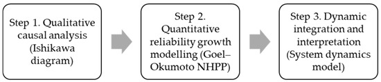
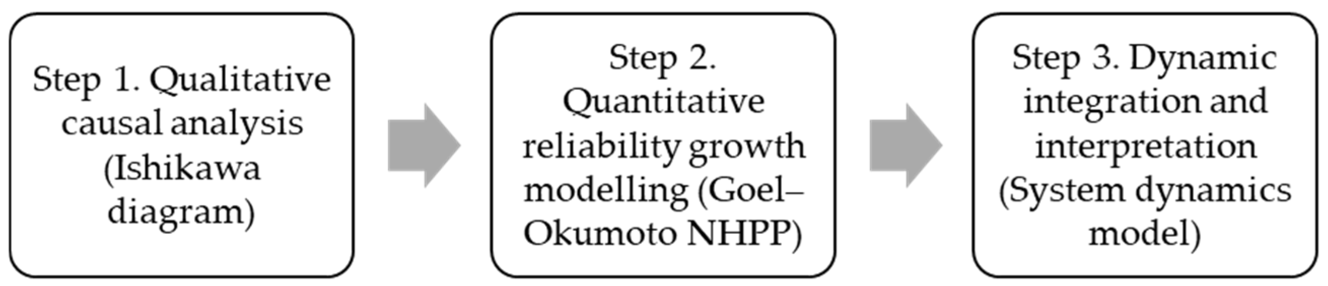
The basis of the analytical framework in this research is the integration of qualitative and quantitative methods in order to foster an in-depth understanding of the potential causes of failures and the dynamics of their occurrence during the utilisation of propulsion gears. The entire process is shown in Figure 1, offering a brief overview of the research methodology and the sequence of events from the identification of possible causes to quantitative descriptions and simulations of system behaviour.

Figure 1. Integrated methodological framework for gear reliability assessment showing the sequential integration of methods: Step 1—qualitative identification of potential failure causes using the Ishikawa diagram; Step 2—quantitative reliability growth modelling based on AMOS maintenance data conducted using the Goel–Okumoto NHPP model and regression analysis; and Step 3—dynamic integration and interpretation of reliability behaviour using a system dynamics model.

As illustrated in Figure 1, the proposed framework follows a sequential integration logic. Qualitative causal analysis provides contextual input for quantitative reliability modelling; this input is subsequently embedded into a system dynamics model to enable dynamic interpretation of reliability behaviour over time.

In the first step, the Ishikawa diagram is used as a qualitative tool to structure potential sources of failure. As the AMOS system does not contain information on human, organisational, or methodological factors, the Ishikawa diagram serves as a framework for systematising potential causes based on the literature, technical documentation, and general engineering principles. Its role in this research is solely qualitative, with the aim of presenting the range of factors possibly impacting the operation of a gear system, without assessing their frequency or statistical relationship.

The second step of the analytical framework is quantitatively modelling failure dynamics by applying the Goel-Okumoto model of reliability growth. This model assesses the cumulative number of failures, failure intensity, and associated NHPP reliability functions based on real data recorded by the AMOS system over 20,000 operating hours. The model parameters are estimated using the least-squares method, and their form provides a description of the typical process in which the number of potential faults is reduced over time.

The third step involves systematic dynamic modelling, providing a simulation and visualisation of the relationships between key variables in the Goel–Okumoto model. In this phase, SDM is used not to add new empirical data but to reproduce the mathematical structure of the model, showing the trends over time and providing a baseline for future scenario analyses and the development of advanced predictive models.

Integrating these approaches leads to a methodological framework that combines a qualitative classification of potential failures, quantitative analysis of actual recorded failures, and simulation-based testing of system behaviour. Figure 1 shows the logical sequence of these steps and their relationships, ensuring there is a clear and consistent research structure. This integration ensures that the applied methods do not operate independently but instead form a unified analytical workflow from empirical data to dynamic reliability interpretation.

2.3. Identification of Failure Causes—Ishikawa Diagram

To qualitatively identify potential causes of failure of the propulsion gear, the cause-and-effect (Ishikawa) diagram method was applied [31]. This method was used as a structured tool for mapping groups of factors that—according to the literature, the technical documentation of the ship propulsion system, and general engineering principles—impact the reliability of gear systems. In this study, the Ishikawa diagram does not represent a quantitative analysis of causes; instead, it functions as a framework for systematising potential sources of failure relevant to subsequent modelling.

Data from the AMOS system were used solely as a source of information on recorded failures, their timestamps, and technical descriptions. As AMOS does not contain detailed data on human, organisational, or methodological errors, causes of this type were included in the Ishikawa diagram based on research from the field of mechanical drives and the standard 6M categories (man, machine, material, method, measurement, and mother nature). Accordingly, the Ishikawa diagram provides a qualitative classification of potential causes rather than a quantitative distribution of causes by categories [31]. It ensures that the diagram covers all relevant groups of factors, although the presence of these factors in the diagram does not imply their frequency in the AMOS logs.

Potential failure causes were grouped according to the following categories [31,32,33]:

• Man—competences, handling procedures, and operational deviations;
• Machine—wear, misalignment, mechanical damage, and adjustment errors;
• Material—quality of steel, lubricants, and consumable parts;
• Method—maintenance procedures, work instructions, inspection, and documentation;
• Measurement—availability and correctness of diagnostic tools and sensors;
• Mother Nature—temperature, humidity, lubricant contamination, and environmental conditions.

The available AMOS data do not allow a quantitative classification of failure causes in percentage terms. While the database provides reliable information on failure occurrence times and technical descriptions, it does not contain structured or standardised fields that would enable consistent attribution of failures to physical, design, manufacturing, operational, maintenance-related, human, or organisational categories. Consequently, the Ishikawa diagram is used solely as a qualitative tool for structuring potential causes rather than for estimating their relative frequency or statistical contribution. The Ishikawa diagram complements the Goel–Okumoto model and the system dynamics simulation qualitatively, providing context and an interpretative basis for understanding potential cause–effect relationships. Given that the method is not quantitative and that the AMOS data do not allow statistical distribution of causes by category, the diagram does not provide information on the frequency or prevalence of specific causes during particular phases of operation, but it does serve as an initial analytical step for systematically mapping possible sources of failures.

2.4. Reliability Growth Model: Goel–Okumoto

The Goel–Okumoto reliability growth model, based on a non-homogeneous Poisson process (NHPP) [26], was applied to quantitatively describe failure dynamics. The model assumes that failures are detected and eliminated during operation and that failure intensity decreases as the number of remaining undetected failures diminishes.

In this model, the expected cumulative number of failures up to time t is defined as follows [26]:

$$m\left(t\right)=a(1-e^{-bt}),$$

(1)

where m(t) is the cumulative number of failures up to time t, a is the expected total number of failures occurring over the life cycle of the system, b denotes the rate at which failure intensity decreases (detection constant), and $e^{-bt}$ is the proportion of failures that remain undetected at time t [26].

The parameters a and b were estimated using ordinary least squares (OLS), in which the sum of squared deviations between the actual cumulative failures from the AMOS database and the model-predicted values was minimised. The minimisation criterion is defined by the following expression:

$$SSE=\sum _{i=1}^n{\left[m_i-a\left(1-e^{-b{t}_i}\right)\right]}^2$$

(2)

The goodness-of-fit of the model was assessed using the sum of squared errors (SSE) and the coefficient of determination (R²). The SSE is the primary criterion for evaluating optimisation quality, while R² assesses the proportion of explained variance relative to the total variability of the data. Based on the estimated parameters, the instantaneous failure intensity is obtained as the derivative of the cumulative failure function,

$$\lambda \left(t\right)={\displaystyle \frac{dm\left(t\right)}{dt}},$$

(3)

and, by substituting the expression for $m\left(t\right)=a(1-e^{-bt})$,

$$\lambda \left(t\right)=ab{e}^{-bt},$$

(4)

which represents the standard NHPP failure intensity function for the Goel–Okumoto model [26].

This expression describes a typical exponentially decelerating failure pattern: failures occur more frequently at the beginning (in the run-in phase), and the rate then decreases as the system stabilises and the underlying causes are progressively eliminated. At the start (t = 0), the failure intensity is maximal (λ(0) = ab). As time goes on, $e^{-bt}$ decreases, and thus failure intensity declines. Accordingly, the model represents a system in which failures are continuously detected and eliminated, with fewer remaining failures over time.

Based on the estimated parameters, additional functions of the model were derived, including the system reliability function obtained from the properties of an NHPP, for which the probability that the system experiences no failures until time t is [10]

$$R\left(t\right)=P\left(N\left(t\right)=0\right)=e^{-m\left(t\right)},$$

(5)

where N(t) is a Poisson random variable with the parameter m(t). All analyses were conducted using AMOS time-series data on cumulative failures.

The rate of change in the reliability function R(t) quantifies the instantaneous rate at which the probability of the system remaining in an operational state decreases over time. In technical systems, analysing ${\displaystyle \frac{dR\left(t\right)}{dt}}$ provides an assessment of failure risk in each phase of a product’s life cycle. This derivative is directly related to failure intensity λ(t), which denotes the instantaneous frequency of failure. In exponential reliability models, this relationship is formally expressed by the equation ${\displaystyle \frac{dR\left(t\right)}{dt}}=\lambda (t)\ast R(t)$, which describes the exponential decay of the reliability function under the influence of the prevailing failure intensity, as shown in Equation (6) [10].

$${\displaystyle \frac{dR\left(t\right)}{dt}}=-\lambda (t)\ast R(t)=-ab{c}^{-b\ast t}\ast R(t)$$

(6)

$$R(t)=e^{-a(1-e^{-b\ast t})}$$

(7)

$$F\left(t\right)=1-R\left(t\right)$$

(8)

$$R\_uk=R\left(t\right)+F\left(t\right)=1$$

(9)

In the reliability literature, the function R(t) represents a key parameter for evaluating system behaviour over time. Its mathematical expression arises from the accumulated risk, that is, the integrated failure intensity λ(t), as given by the following relation. Equation (6) shows the rate of change in the reliability function over time. The derivative ${\displaystyle \frac{dR\left(t\right)}{dt}}$ is proportional to the instantaneous failure intensity λ(t) and the current reliability R(t). The negative sign indicates that reliability decreases as the probability of failure F(t) for the system increases over time, as shown in Equation (8) [10]. The total system reliability is given by Equation (9) [34,35]. All analyses were performed using the time-series failure data from the AMOS database, and the calculated values of m(t), λ(t), and R(t) were used in subsequent stages of the analysis. Importantly, the applied reliability growth model assumes that each detected and corrected failure permanently reduces the number of potential failures remaining, resulting in a monotonically decreasing failure intensity. This assumption implies that maintenance actions are fully effective and do not introduce new faults into the system. In real ship operating conditions, this may not always be the case, as certain maintenance interventions may have limited effectiveness or even introduce new failure mechanisms. These effects are not explicitly modelled in the present study and represent a deliberate simplification adopted to ensure analytical transparency.

2.5. System Dynamics Simulation Model

The system dynamics model is not intended to increase numerical complexity or replace analytical reliability-growth modelling. Instead, it serves as an integrative layer that embeds the analytically estimated Goel–Okumoto model parameters into a dynamic structure, enabling transparent interpretation of reliability evolution over time and providing a foundation for future scenario-based extensions. To present the interdependencies among technical, operational, and environmental variables and simulate the dynamics of failures over time, a system dynamics simulation model (SDM) was developed using POWERSIM Studio PowerSim Constructor 2.5.d (4002) software. The system dynamics approach models accumulations, flows, and feedback loops that regulate system behaviour over long time horizons [36].

The model consists of three fundamental elements [34,35,36]:

• Stocks, representing accumulated system variables (the number of active failures, reliability level, etc.);
• Flows, representing state changes (e.g., detection and removal of failures);
• Feedback loops, linking outcomes to input variables and enabling dynamic system adjustment.

The model incorporates the mathematical structure of the Goel–Okumoto model in order to quantitatively describe the dynamics of fault occurrences. The values of the functions are used as input variables in the simulation flows. Additional variables include operating conditions, such as temperature, load, and the maintenance interval [37], as well as operating factors, which impact the rate of fault identification and elimination. Furthermore, the system dynamics model does not incorporate explicit maintenance feedback effects, such as imperfect repairs, maintenance-induced failures, or changes in failure behaviour resulting from operational or organisational decisions. The dynamic structure is therefore limited to reproducing the reliability growth behaviour implied by the analytical model, while more complex maintenance feedback mechanisms are identified as a direction for future research.

While the analytical reliability growth model provides explicit analytical expressions for failure intensity and reliability, the system dynamics implementation is used to generate simulation results that reproduce these relationships over time and enable a structured interpretation of their dynamic behaviour.

2.6. Regression Analysis

Regression analysis was used to numerically verify the consistency of the system dynamics model and verify that the relationship between simulated variables stems from the analytical pattern defined in the Goel–Okumoto model. Given that the simulation model generates a set of deterministically related variables, the purpose of regression is not to test the statistical significance coefficient but to verify the stability and regularity of the mathematical relationship between failure intensity and the reliability function.

Our analysis accounted for the relationship between the following variables: cumulative failure intensity (dmt), instantaneous failure intensity (dLam), reliability intensity (dRt), and unreliability intensity (dFt). For each pair of variables, a dedicated regression equation was formulated in order to test the agreement between simulated values and expected functional relationships from the NHPP framework.

The regression model was formulated in the general linear form:

$$y={\beta }_0+{\beta }_{1}x+\epsilon$$

(10)

where y is the dependent variable, x is the independent variable from the analysed pair, β₀ and β₁ are the regression coefficients estimated using the ordinary least squares (OLS) method, and ε is the random error.

The goodness-of-fit model was evaluated using the determination coefficient (R²) and correlation coefficient (r), with the aim of evaluating the extent to which the simulated relationships reflect the theoretical patterns of reliability growth [38]. This approach helps us evaluate the exactness of the underlying structure of the system dynamics model and its conformance to the mathematical properties of the Goel–Okumoto model. The presented system dynamics model was used to simulate the temporal evolution of failure intensity and reliability based on empirically estimated model parameters.

A comprehensive analysis of propulsion-gear failures based on the presented methods and collected data was performed. The next chapter presents the results of identifying the causes of failures, parameter estimation of the Goel–Okumoto model, the system dynamics simulation, and regression analysis. The results provide insight into the dominant factors affecting gear reliability and the dynamics of failure occurrence over 20,000 operating hours.

3. Results

This section presents the results obtained from the integrated analytical and simulation-based reliability assessment framework. The results were derived from the system dynamics simulation, which embedded the analytically estimated Goel–Okumoto model parameters based on empirical AMOS data. The presented outputs therefore reflect both the analytical reliability-growth formulation and its dynamic simulation over time.

3.1. Ishikawa Diagram

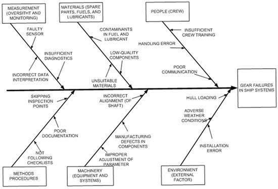
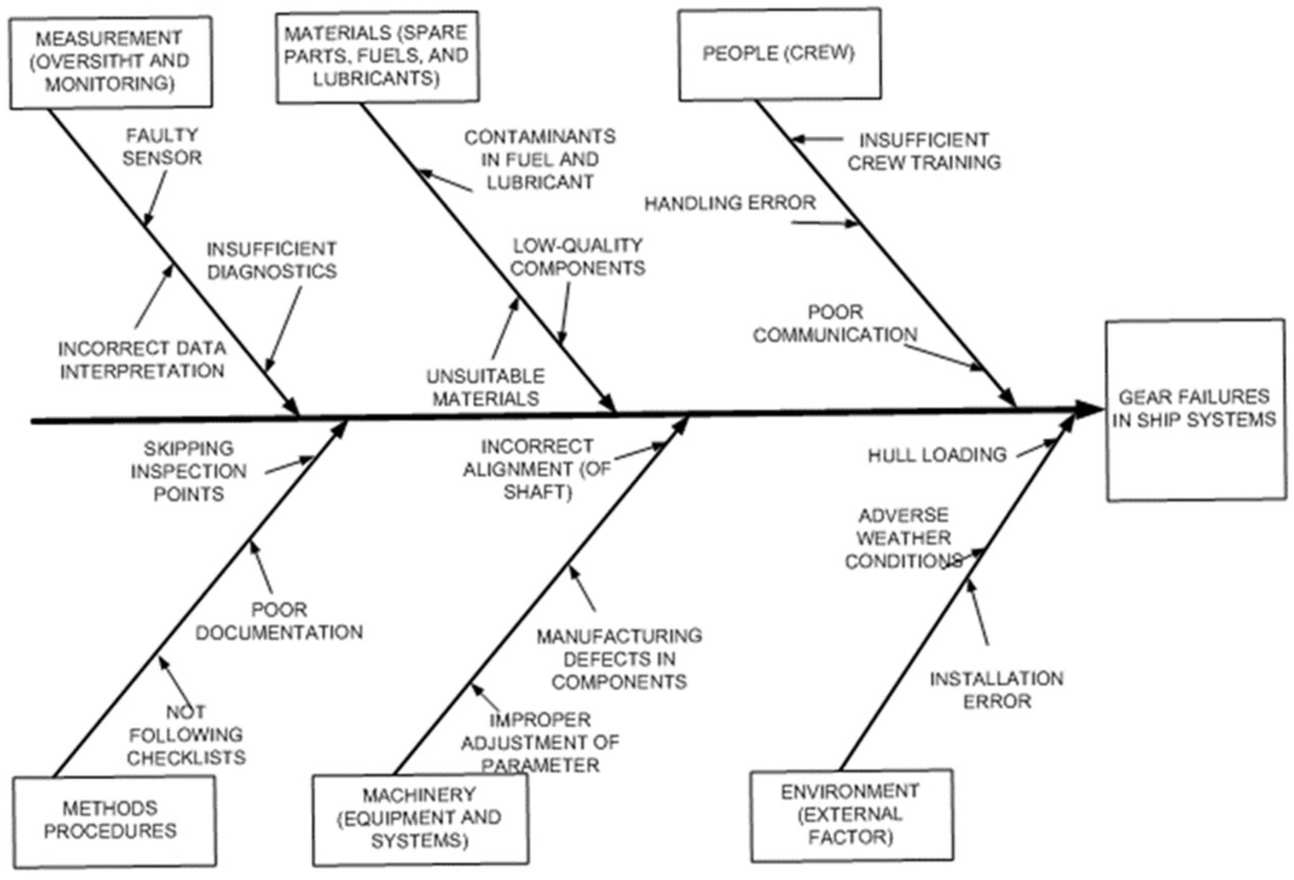
Based on the qualitative framework presented in Section 3.3, an Ishikawa diagram was devised to systematise the potential sources of propulsion gear failures according to the standard 6M model (people, machinery, materials, methods, measurement, and environment) [31]. The categories and corresponding potential causes are given in Table 3, with the mechanical properties and surface durability of gears as defined in ISO 6336-2 guidelines [39].

Table 3. Categories and typical potential causes of gear failure [40,41].

Category	Typical Failure Causes
People (Crew)	Insufficient training, handling errors, inattentiveness, and poor communication
Machinery	Shaft misalignment, gear-tooth wear, and poorly adjusted operating parameters
Materials	Low-quality steel, inadequate lubricants, and surface fatigue of materials
Methods	Insufficient documentation, inaccurate checklists, and lack of corrective feedback
Measurement	Faulty vibration sensors and lack of diagnostic equipment
Environment	Elevated temperature and humidity and contamination of lubricant by seawater

The Ishikawa diagram (Figure 2) is a structural representation of possible cause–effect relationships; however, it does not provide information about the relative frequency of failures or the order in which they occurred. These limitations arise from the fact that AMOS logs do not contain detailed information on human, methodological, or organisational causes; thus, the Ishikawa diagram was primarily used as a qualitative support tool for contextualising the mathematical and simulation results.

Figure 2. Ishikawa diagram of gear failures in ship systems.

In this analytical study, the Ishikawa diagram provides insight into the range of potential causes of failure, whereas the quantitative dynamics modelling of failures is based only on empirical data (the Goel–Okumoto model) and simulation results (the SD model). Accordingly, the Ishikawa diagram complements, but does not determine, the numerical outcomes of the reliability model.

3.2. Application of the Goel–Okumoto Model to Gear Failures

The Goel–Okumoto model was applied to real data on gear failures recorded over 20,000 operating hours. Table 4 compares the actual and modelled cumulative number of failures, along with the squared error at each time point. To assess the Goel–Okumoto model’s goodness of fit with respect to the empirical data, parameters a and b were estimated, and the corresponding accuracy indicators (SSE and R²) were calculated, providing an objective comparison of the modelled and actual failure values.

Table 4. Prediction of the cumulative number of failures obtained using the Goel–Okumoto model.

Time	New Failure	Cumulative Failures (Actual)	m(t) GO Model	Squared Error
2000	5	5	5.22	0.05
4000	4	9	9.23	0.08
6000	4	13	12.43	0.33
8000	2	15	14.88	0.01
10,000	2	17	16.78	0.05
12,000	1	18	18.26	0.07
14,000	1	19	19.41	0.17
16,000	1	20	20.30	0.09
18,000	1	21	21.00	0.00
20,000	1	22	21.54	0.21

Critically, the Goel–Okumoto model is calibrated on the cumulative failure function m(t), not on the number of newly recorded failures within individual time intervals. Parameters are estimated using ordinary least squares (OLS) by minimising the deviation between the observed cumulative failures and the corresponding model values. Therefore, short-term variations in the number of failures, especially during the run-in phase, are not expected to be reproduced exactly. The higher greater of failures observed in early intervals reflects the discrete character of real operational events, whereas the model describes the overall decreasing trend typical of reliability growth. The agreement between empirical and modelled values is therefore evaluated at the cumulative level, an approach consistent with the underlying non-homogeneous Poisson process formulation. Table 4 shows that the modelled values m(t) correlate well with the actual cumulative failures, with small deviations at most points. The largest individual error occurs at 6000 operating hours, but it remains low in terms of absolute magnitude.

The model parameters were estimated using OLS, and their values and the total squared error are given in Table 5.

Table 5. Estimated parameters of the Goel–Okumoto model and goodness-of-fit indicators.

Quantity	Designation	Value
Total expected number of failures	a	23.42
Detection-rate parameter	b	0.000126
Sum of squared errors	SSE	1.06
Coefficient of determination	R2	0.9962

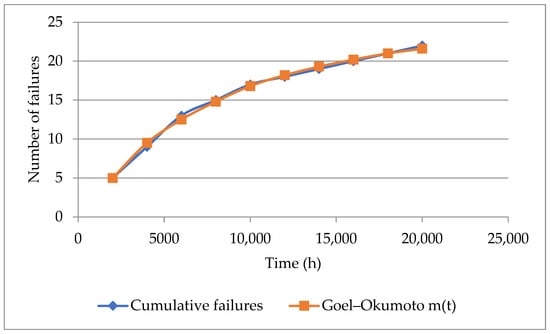
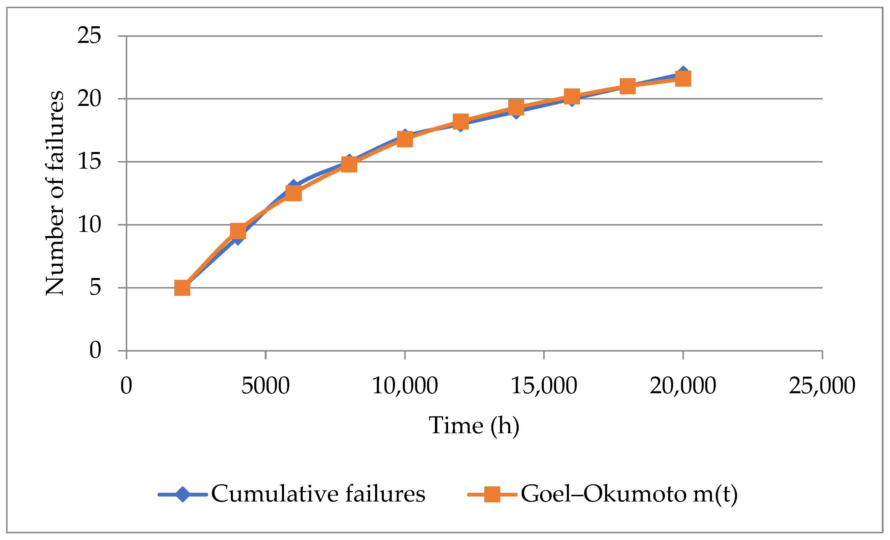
The obtained SSE value of 1.06, for cumulative failures in the order of 20–30, indicates very good agreement between the model and the data. It should be noted that the high R² value reflects the consistency of the model with the available dataset rather than its generalisation capability beyond the observed operating period. A graphical comparison of the actual and modelled cumulative failures is shown in Figure 3. The observed decrease in failure intensity is consistent with the stabilisation phase of gear operation rather than long-term wear-out behaviour.

Figure 3. Comparison of actual cumulative failures and the Goel–Okumoto model prediction.

The model curve follows the general trend of the data, showing an initially faster increase (run-in phase) and a gradual flattening in the later stage, with an asymptote around a ≈ 23.

Based on the estimated parameters, the values of failure intensity λ(t) and the reliability function R(t) were calculated at representative time points. The results are given in Table 6.

Table 6. Failure intensity λ(t) and reliability R(t).

Failure Intensity λ(t)	Reliability R(t)
0.00229	0.017308247
0.00178	0.042759073
0.00139	0.086344690
0.00108	0.149072694
0.00084	0.227869418
0.00065	0.316874759
0.00051	0.409414258
0.00039	0.499608531
0.00031	0.583202323
0.00024	0.657701767

The results reveal an exponential decrease in failure intensity λ(t) over time, consistent with the model’s assumption that the number of undetected failures remaining decreases as the system stabilises. At the same time, the NHPP-based reliability R(t) increases toward its asymptote within the observed time horizon.

The value R(20,000) ≈ 0.66 indicates that the modelled probability of no new failures occurring by the end of the observation interval is approximately 66%. This value refers to the stochastic process of failure detection rather than the physical condition or material integrity of the gear. Accordingly, the obtained reliability values describe the dynamics of the reliability growth process and should not be interpreted as an absolute indicator of component health or wear.

The Goel–Okumoto model provides quantitative insight into failure dynamics based on real AMOS data and is the basis for further integration in alignment with the dynamic simulation of the system dynamics model.

3.3. Results of the System Dynamics Model Simulation

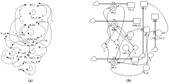
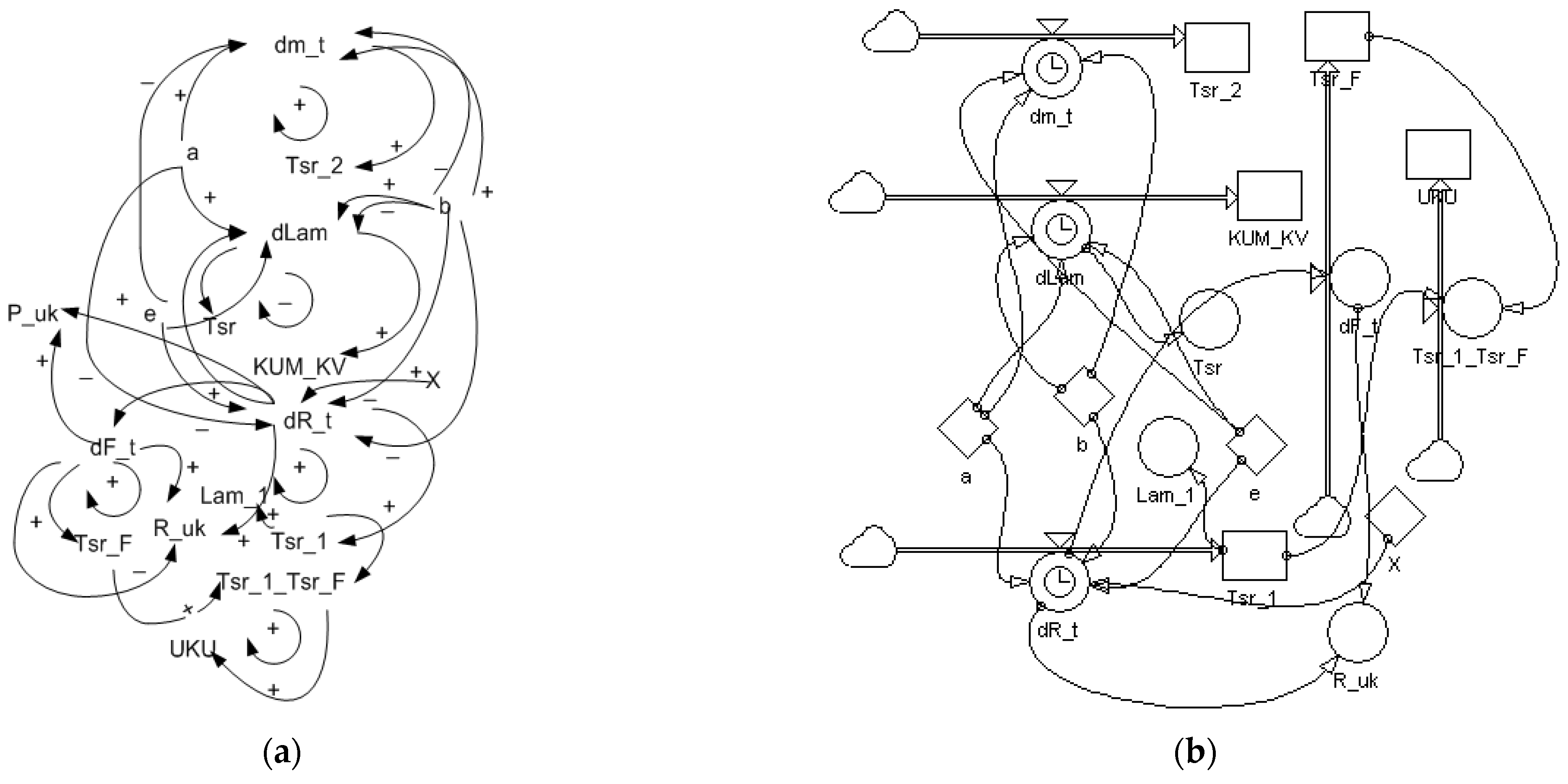
Based on the Goel–Okumoto equations and expressions for failure intensities and reliability, a system dynamics model was developed in POWERSIM. Figure 4a shows the conceptual system dynamics model (cause–effect relationships), while Figure 4b presents the implemented model using POWERSIM notation. In the system dynamics representation, cumulative detected failures are modelled as stock variables, while the failure detection process is represented as a flow variable governed by the Goel–Okumoto failure intensity function. Reliability is treated as a derived variable obtained from the cumulative failure process. This structure ensures consistency between the analytical reliability-growth model and its dynamic implementation.

Figure 4. System dynamics representation of the Goel–Okumoto reliability growth model for propulsion gears: (a) conceptual causal structure of the qualitative system dynamics model and (b) quantitative implementation in POWERSIM. The cumulative number of detected failures (KUM_KV) is modelled as a stock variable driven by the failure detection flow (dm_t), while the failure intensity (dLam) is defined by Goel–Okumoto parameters a and b.

Figure 4 illustrates the internal logic of the proposed system dynamics model. In the conceptual representation (Figure 4a), the cumulative number of detected failures (KUM_KV) is modelled as a central stock variable whose rate of change is governed by the failure detection flow (dm_t). Failure intensity (dLam), corresponding to the analytical failure rate λ(t), is represented as an auxiliary variable that influences the rate at which failures are detected over time. Figure 4b presents the quantitative implementation of the same structure in the POWERSIM simulation environment. In this formulation, KUM_KV is implemented as a stock variable with dm_t as its inflow, while the failure intensity dLam is calculated internally based on the fixed Goel–Okumoto parameters a and b and directly governs the magnitude of the failure detection flow. System reliability and unreliability are implemented as derived variables linked to the cumulative failure process, preserving the analytical NHPP relationships and maintaining the condition R(t) + F(t) = 1. The system dynamics model does not introduce additional assumptions or maintenance feedback mechanisms; instead, it provides a transparent dynamic representation of the analytical reliability growth model and a foundation for future extensions involving operational or maintenance-related feedback.

The simulation was conducted over 20,000 operating hours, in increments of 2000 h. Table 7 outlines the main simulation results (reliability and unreliability functions and derived quantities) for selected time points.

Table 7. Examples of simulated values of the reliability and unreliability functions (POWERSIM).

Time	dm_t	dLam	dR_t	dF_t	Tsr_1	Tsr_1_Tsr_F	R_uk	Tsr_F
0	0.00	0.00295	0.777	0.223	0.00	0.00	1.00	0.00
2000	5.22	0.00229	0.604	0.396	1373.77	2000.00	1.00	626.23
4000	9.28	0.00178	0.469	0.531	2441.35	4000.00	1.00	1558.65
6000	12.43	0.00138	0.365	0.635	3270.99	6000.00	1.00	2729.01
8000	14.88	0.00108	0.283	0.717	3915.73	8000.00	1.00	4084.27
10,000	16.78	0.000836	0.22	0.78	4416.76	10,000.00	1.00	5583.24
12,000	18.26	0.00065	0.171	0.829	4806.12	12,000.00	1.00	7193.88
14,000	19.41	0.000505	0.133	0.867	5108.70	14,000.00	1.00	8891.30
16,000	20.30	0.000393	0.103	0.897	5343.85	16,000.00	1.00	10,656.2
18,000	21.00	0.000305	0.0803	0.92	5556.58	18,000.00	1.00	12,473.4
20,000	21.54	0.000237	0.0624	0.938	5668.58	20,000.00	1.00	14,331.4

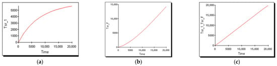
Table 7 presents selected simulated values obtained from the system dynamics model implemented in POWERSIM. The variables shown represent time-dependent outputs derived from the analytical Goel–Okumoto reliability growth formulation and its dynamic implementation. The failure detection flow (dm_t) and failure intensity (dLam) describe the decreasing rate of newly detected failures over time, while the reliability and unreliability rates (dR_t and dF_t) quantify the corresponding changes in system reliability. The accumulated operating time (Tsr_1), downtime (Tsr_f), and total observed time (Tsr_1_Tsr_F) are auxiliary variables included to support interpretation of reliability behaviour in relation to system availability. The total system reliability (R_uk = R(t) + F(t)) remains equal to unity throughout the simulation, confirming the numerical and structural consistency of the system dynamics model.

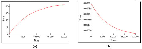
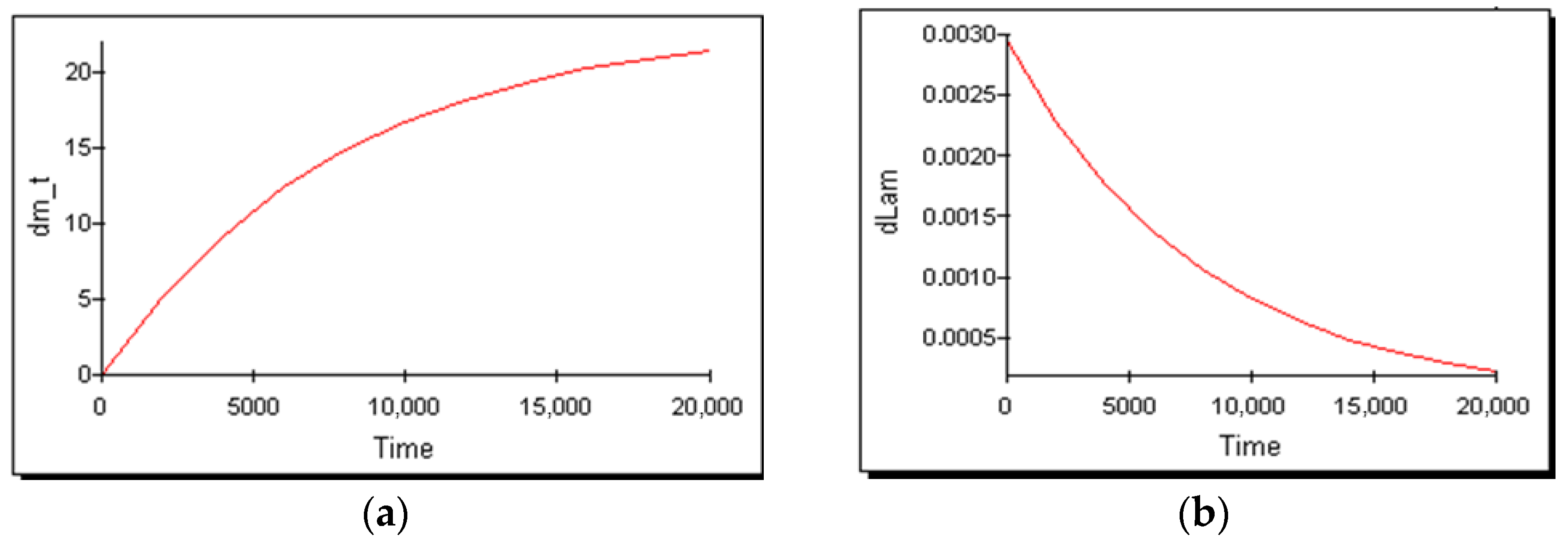
The simulation results are illustrated in Figure 5 and Figure 6. Figure 5a presents the intensity of cumulative failures, dm_t, indicating the typical form of exponential saturation, characterised by a rapid initial increase and a slowdown in the later stage. In Figure 5b, the failure intensity dλ(t) decreases exponentially, consistent with the analytical expression $\lambda \left(t\right)=ab{e}^{-bt}$, indicating system stabilisation over time.

Figure 5. Intensity of cumulative failures (a) and failure intensity (b) in the SD model.

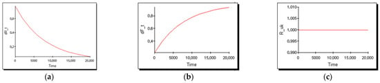
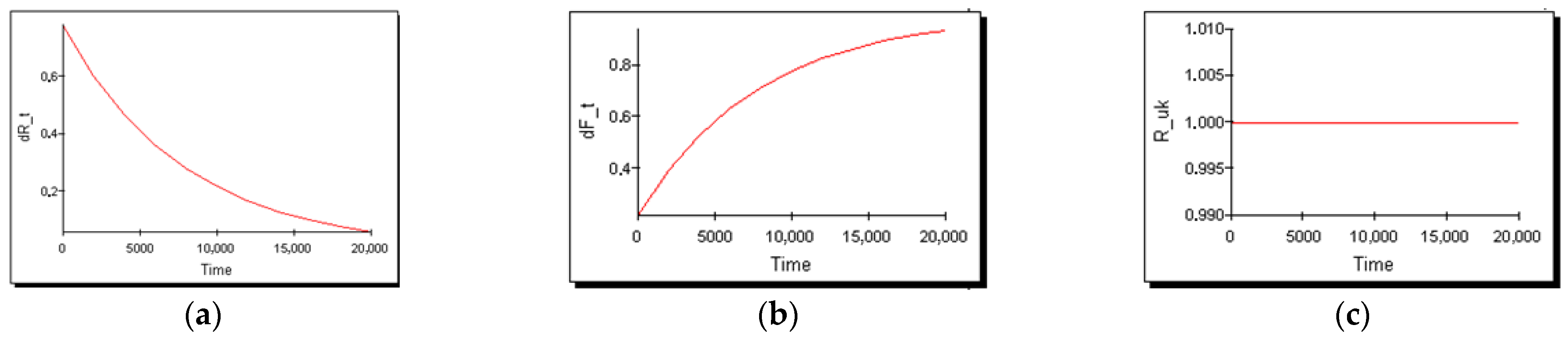
Figure 6. Dynamics of changes in (a) the derivative of the reliability function; (b) the derivative of the unreliability function; and (c) the sum of the reliability and unreliability intensities.

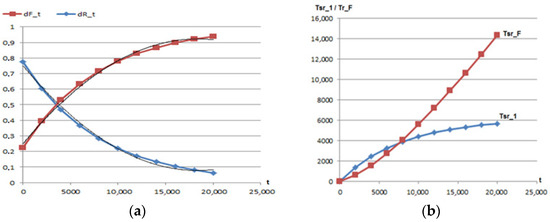
Figure 6 shows the derivatives of the reliability and unreliability functions. Figure 6a displays the derivative of the reliability function, dR(t)/dt, which is negative and decreases in absolute value, indicating a progressively slower reduction in reliability as the system stabilises. Figure 6b shows the derivative of the unreliability function, dF(t)/dt, increasing to a certain level and then stabilising and corresponding to the expected behaviour of the system over its life cycle. Figure 6c shows the sum of the reliability and unreliability intensities, which remains constant, confirming the internal consistency of the model.

Furthermore, after assessing the failure intensity and reliability function, we considered the mean time between failures (MTBF), which serves as a key indicator of long-term system operational stability. The value of the mean time to failure (MTTF) was calculated based on the results of the model simulation, which used the analytically defined function λ(t) and R(t) from the Goel–Okumoto model. The MTTF is presented by the integral function of reliability over time:

$$MTTF={\int }_0^{\infty }R\left(t\right)dt$$

(11)

The obtained parameter values of the model (a = 23.42; b = 0.000126) were used to calculate the value of the MTTF, which amounted to approximately 870 h, which is the average time interval between two more significant failures of the gear in the system analysed. Our analysis shows a characteristic pattern of three-phase behaviour within mechanical systems.

• Run-in phase (0–5000 h): The MTTF is lower due to the increased occurrence of early failures.
• Stable operation phase (5000–15,000 h): The MTTF reaches its highest values (≈12,000 h).
• Initial degradation phase (>15,000 h): The MTTF slightly decreases again, consistent with expected material fatigue and lubricant degradation.

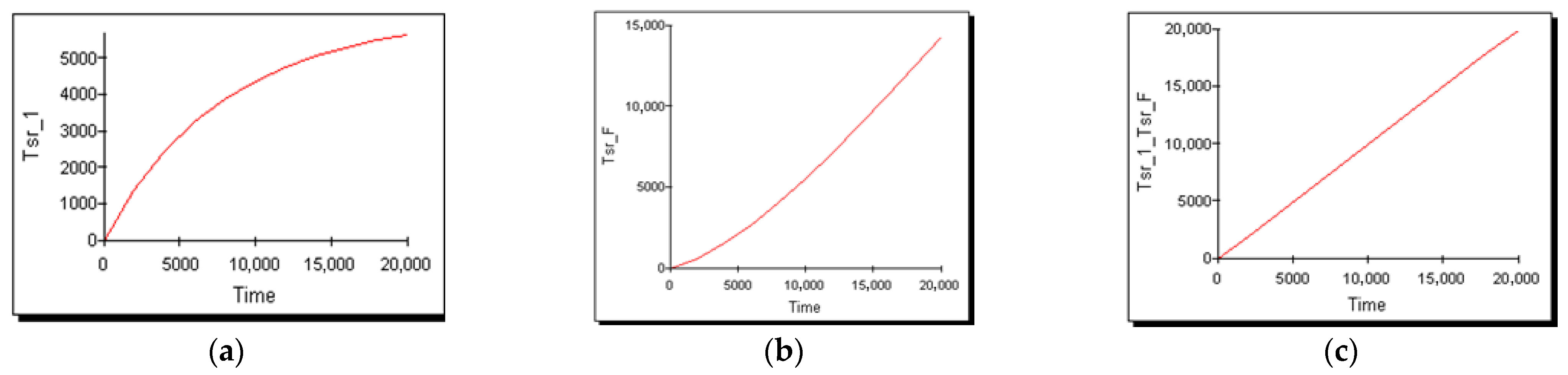
The mean time to failure (MTTF) and mean time in failure were analysed based on the results of the simulation. Figure 7a–c show the dynamics of the MTTF, the mean time in failure, and their total sum. The resulting trends confirm the coherence of the mathematical model and the simulation outputs and allow detailed monitoring of reliability changes throughout the system’s entire life cycle.

Figure 7. (a) Mean time of gear operation; (b) mean time in failure increases more rapidly than the mean time in operation; and (c) the sum of the mean time in operation and the mean time in failure mode.

According to Figure 7a, the mean time to failure (MTTF) for gear operation increases and approaches a limiting value, with a rapid rise in the initial operating phase and a gradual saturation in the later stage. This behaviour is characteristic of systems in which a stable operating regime is quickly established and performance becomes clearly recognisable [34,35]. According to Figure 7b, the mean time in failure increases more rapidly than the mean time in operation, indicating a higher maintenance burden in the late phase of the life cycle. According to Figure 7c, the sum of the mean time in operation and the mean time in failure mode is equivalent to the total observed time, indicating the consistency of the availability model.

This pattern suggests that a stable operating regime is achieved in the early operating phase, whereas in later phases, an increasing amount of time is lost due to intervention periods. This information is relevant when making plans regarding the maintenance and availability of propulsion systems.

The system dynamics model visualises the relationship between the technical and operational variables that impact the reliability of gears over their lifespan [34]. The simulation conducted for a time horizon of 20,000 operating hours showed that the reliability function R(t) increases during the initial operating phases of the system and achieves a stable zone at around 12,000 h, after which gradual stagnation is recorded. This pattern conforms to the expected dynamics of mechanical systems, where after the run-in and corrective maintenance action phases, the effects of long-term material fatigue arise. A comparison of the simulated values R(t) with the empirical data from the AMOS database shows a high correlation, confirming that the model adequately describes the observed system. The simulation is used solely to present the fundamental dynamics of reliability, without conducting scenario analyses of maintenance, whereby, consequently, the results reflect the system’s behaviour under conditions recorded in the available data.

The system dynamics model is designed to remain fully consistent with the analytically derived reliability growth relationships, with failure intensity and cumulative failures represented through flow and stock variables. While the analytical reliability-growth model provides explicit analytical expressions of failure intensity and reliability, the system dynamics implementation offers a flexible representation of these relationships for potential future extensions.

3.4. Regression Analysis of the SD Results

Based on the simulation results derived from POWERSIM PowerSim Constructor 2.5.d (4002) software, a regression analysis was conducted to test for relationships between key variables in the model: cumulative failure intensity, instantaneous failure intensity, reliability intensity, and unreliability intensity. The aim of these analyses was to estimate the level of mutual links between the simulation parameters and confirm the consistency of the model’s structure.

The regression results in Table 8 show a very high coefficient of determination (R² ≈ 0.99–1.00), indicating an almost perfect correlation between simulation values and the regression functions. This outcome confirms that the simulation relationships between the variables follow the expected mathematical patterns and that the model is stable in its numerical interpretation.

Table 8. Regression equations, coefficients of determination, and correlation coefficients for the SD model.

Relation Y = f(t)	Regression Equation	R2	r
dm_t/dR_t	Y1 = −30.13X + 23.414	1	1
dLam_t/dR_t	Y2 = 0.0038X + 0.000001	1	1
dR_t	Y3 = −0.000000002 × X2 + 0.00007 × X − 0.2495	0.9951	0.9975
dF_t	Y4 = 0.000000002 × X2 − 0.00007 × X + 0.2495	0.9951	0.9975

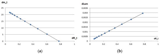
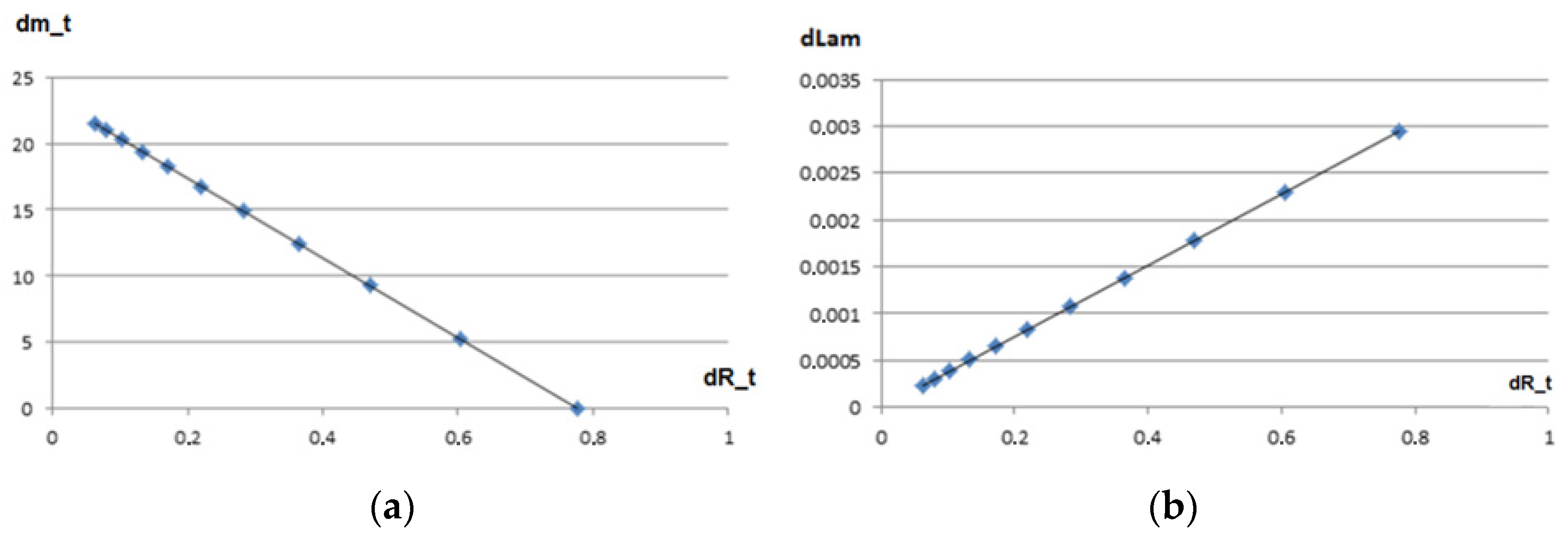
Analysis of the relationship between the intensity of cumulative failures and reliability intensity (Figure 8a) shows a strong negative linear relationship: as reliability increases, the overall intensity of failures decreases. The relationship between failure intensity and reliability intensity (Figure 8b) is positive and linear, confirming that changes in instantaneous failure frequency directly affect reliability.

Figure 8. Relationships in the system dynamics model: (a) the relationship between the intensity of cumulative failures and reliability intensity, and (b) the relationship between failure intensity and reliability intensity.

A strong non-linear but almost perfectly inverse relationship was also observed between reliability intensity and unreliability intensity (Figure 9a), a finding consistent with the theoretical assumptions of the model. Furthermore, the relationship between the mean time in operation and the mean time in failure (Figure 9b) confirms there is predictable and consistent system development over time.

Figure 9. Relationships between (a) unreliability intensity, reliability intensity, and (b) mean operating times in the system dynamics model.

The results indicate that the simulation model behaves in accordance with the analytical equations and that there are stable, statistically strong relationships between the key variables. These findings confirm that the system dynamics model authentically replicates the reliability dynamics of mechanical systems based on the Goel–Okumoto model and is a reliable basis for further interpretation and maintenance planning.

3.5. Integration of Analytical, Simulation, and Regression Results

An integrated analysis of the results obtained using the Goel–Okumoto model, system dynamics simulations, and regression analysis of the simulation data was conducted to assess the stability of the reliability model and verify the consistency of the analytical approaches. In this step, we confirmed the model is internally consistent and evaluated its suitability for describing the real behaviour of gears in ship propulsion systems.

The analytical Goel–Okumoto model shows that the cumulative number of failures m(t) follows an exponential saturation trend, with a decreasing failure intensity λ(t) over time. These results were fully reproduced in the system dynamics model, in which the simulated values d m(t), d λ(t), and R(t) showed the same patterns (Figure 5 and Figure 6). The simulated data verified the run-in phase, the stable mid-period, and the onset of degradation at approximately 15,000 h of operation, consistent with the analytical estimates and MTTF values.

The regression analysis further confirmed the model’s consistency. We observed a strong negative relationship between the intensity of cumulative failures and reliability intensity (Figure 8a), a strong positive relationship between failure intensity and changes in reliability (Figure 8b), and an almost-perfect inverse relationship between reliability and unreliability intensities (Figure 9a). Finally, analysis of the mean time in operation and mean time in failure (Figure 9b) demonstrated a stable, predictable relationship, confirming the consistency of the availability model.

Integrating the analytical, simulation, and regression results shows that all the approaches applied consistently describe system reliability. The correlation of trends and the strong statistical relationships confirm that the model reliably reflects gear behaviour in operation and can serve as the basis for maintenance planning and assessing the long-term operational stability of ship propulsion systems. Together, these results demonstrate that the theoretical formulation is directly operationalised through simulation and regression analysis, providing a detailed and internally consistent representation of gear reliability dynamics under real operating conditions.

4. Discussion

The research results confirm that integrating qualitative and quantitative approaches provides comprehensive and interpretable insight into gear reliability under real ship operating conditions. The application of the Goel–Okumoto model proved suitable for describing the dynamics of failure detection based on AMOS system data, with the very high degree of agreement between the model and the empirical data (R² = 0.9962) confirming that non-homogeneous Poisson processes (NHPPs) can properly describe typical reliability-growth patterns in technical systems in which failures are gradually eliminated.

The model parameters obtained (a = 23.42, and b = 0.000126) reflect a typical process in which initial failure rates are higher, followed by a gradual decrease as the system stabilises. This trend is consistent with earlier studies on ship systems, which describe an initial phase characterised by a higher occurrence of early failures followed by a transition to a stable operating regime [42,43].

The system dynamics model supplemented the analytical approach, providing a visual and structured presentation of the relationships between instantaneous failure intensity, cumulative failure, and the NHPP-based reliability of time. Though the SD model in this stage of the research does not provide additional empirical data, its function is twofold: it confirms the mathematical consistency of the Goel–Okumoto model using a simulation environment and (2) provides a future upgrade using operating and environmental variables that can be tracked in real time. Therefore, the SDM can serve as the basis for building dynamic predictive tools and potential digital twin models for ship propulsion systems. From a practical perspective, sensitivity to the parameters a and b highlights the importance of accurate failure recording and parameter estimation, as small changes in these values can significantly affect predicted reliability trends.

It should be noted that the Ishikawa diagram for the operation mode plays a qualitative role. Given that the AMOS system does not contain human, organisational, or methodological causes, the diagram is used for the systematisation of potential factors according to the 6M classification, not for a quantitative estimate of their frequency. In this way, a broader context is given for the analytical results, providing a better understanding of possible sources of failure, although the conclusions on the dynamics of failures are based solely on empirical data and mathematical modelling.

Our regression analysis provides numerical verification of the consistency of the simulation model rather than a classical statistical analysis. Given that the simulated variables are deterministically linked in mathematical equations, the high values for the coefficients of determination were expected and confirm that the SDM accurately reproduces the structure of the NHPP model. This further confirms the stability and credibility of the integrated approach.

In a broader context, the results of this study align with recent trends in reliability analysis of maritime systems, which increasingly rely on integrating physical models, maintenance data, and simulation tools. In this way, the devised framework has potential applications in predictive maintenance, optimisation of service intervals, and decision support in ship propulsion. The model can be integrated into existing maintenance management systems (e.g., AMOS), enabling real-time monitoring of reliability growth.

4.1. Theoretical Implications

The integrated approach used in this study has important theoretical implications, confirming that models of reliability growth based on non-homogeneous Poisson processes can be applied to gears in ship propulsion systems, where failures are relatively rare but exhibit a clearly defined frequency of occurrence. After applying the Goel–Okumoto model, we observed that its analytical patterns closely match the real data recorded in the AMOS system, thereby confirming the theoretical feasibility of using the model for marine mechanical components. Integrating the qualitative Ishikawa diagram, the Goel–Okumoto model, and system dynamics modelling provides a conceptual and methodological coherent framework, linking the structure of potential causes with a quantitative representation of failure dynamics. This contributes to the current literature, which has traditionally analysed these aspects separately, and opens the path for future research, combining qualitative and quantitative approaches in estimating technical reliability. Additionally, the clear distinction between reliability in general and the physical reliability of materials is theoretically important, as it fosters a more precise interpretation of the results and prevents erroneous interpretation of failure identification processes as a property of materials. The system dynamics model offers additional theoretical value as it shows how the parameters of the Goel–Okumoto model can be transferred into a simulation environment, further allowing the upgrading and analysis of scenarios, constituting the basis of developing predictive and adaptive models of reliability.

4.2. Practical Implications

The practical implications of the research results are especially important for the operational maintenance management of ship propulsion systems. The reliability growth model offers a more precise insight into failure dynamics during exploitation, which can, in turn, improve the planning of service intervals and enable a transition from stasis to strategies in terms of foreseeing maintenance periods. Integrating the model into systems such as AMOS makes it possible to estimate, in real time, the current position of the system on the reliability growth curve and envisage when the risk of a new failure will increase. Consequently, support in decision-making across technical departments improves and allows for the optimisation of resource allocation, overhaul times, and project priorities. The system dynamics component of the model further enables consideration of future scenarios, including changes to operating and environmental conditions, an ability that is especially useful for serial ships and their systems. Though the Ishikawa diagram in this research does not quantify the frequency of failures, it nonetheless provides valuable insight into potential areas in which deviations can occur; this insight can, in turn, can serve as the basis for revising maintenance procedures and improving operating documentation and methodologies for identifying risks. Overall, this integrated approach shows that the combination of data from the maintenance system, mathematical modelling, and simulation tools fosters a deeper understanding of the behaviour of propulsion components in real conditions and is a valuable step towards advanced methods for predictive maintenance.

4.3. Limitations and Directions for Future Research

Although the analysed dataset only spans 20,000 operating hours, which may be insufficient to capture the wear-out phase of gear life, it reflects realistic operational periods commonly available in ship maintenance databases and is therefore appropriate for reliability growth analysis during early and stable operation. Despite these valuable findings, this study has a number of limitations affecting the scope of the applicability of the results. The relatively small number of observed failure events (N = 22) represents a limitation of this study and may have contributed to the high goodness-of-fit indicators obtained for the reliability growth model. While the high R² value indicates strong agreement between the model and the available data, it should be interpreted in the context of the limited sample size and the restricted observation period. This analysis is based on a limited number of failures and on data from only a single ship. Such conditions do not allow generalisation of the results without additional empirical validation. The data available from the AMOS system do not contain standardised or sufficiently detailed information on organisational, human, or methodological causes, preventing quantitative classification of failure causes by category. Consequently, the Ishikawa diagram has a purely qualitative role and cannot be used to estimate the frequency or prevalence of specific causal categories over a component’s life cycle. Although the system dynamics model is useful for checking consistency and visualising processes, it does not, at this stage, incorporate operational or environmental variables that may significantly influence system behaviour under real operating conditions. In addition, predicting failure probability during the accelerated wear-out phase would require long-term operational data that capture increasing failure intensity and is therefore beyond the scope of this study.

Given the identified limitations, future research should focus on expanding the dataset by including more vessels and longer periods of operation, more robustly estimating the Goel–Okumoto model parameters, and increasing the reliability of the conclusions. Additionally, incorporating sensor data, such as through vibration, temperature, oil, and load analysis, would allow the model to be further developed toward predictive and adaptive reliability-monitoring systems, including the creation of digital twins for ship propulsion components. The system dynamics model could also be upgraded by adding variables that represent changes in the operating conditions and decisions on maintenance, thereby creating a tool for simulating various scenarios and the optimisation of service strategies. Finally, by combining the Goel–Okumoto model with mechanical engineering methods for diagnostics and algorithms for machine learning, a significantly more precise prediction of failures could be possible, including with respect to support for decision-making in real time. Future versions of the proposed framework should explicitly account for imperfect maintenance actions, maintenance-induced failures, and feedback effects between maintenance decisions and system reliability.

5. Conclusions

This study confirms that reliability growth modelling can be consistently applied to propulsion gear systems using real maintenance records. The main contribution lies in the integration of qualitative cause structuring, NHPP-based reliability growth modelling, and system dynamics representation within a single analytical framework. These elements are not analysed separately; they are connected in a structured manner that links empirical maintenance data with an interpretable description of reliability evolution over time.

The significance of this work lies in demonstrating that reliability growth concepts can be transferred to marine propulsion components using standard maintenance documentation. The results show that even a limited but well-defined dataset can provide meaningful insight into stabilisation behaviour and failure dynamics during the early and stable phases of operation. In this way, this study contributes to connecting theoretical reliability modelling with shipboard maintenance practices.

From a practical standpoint, this framework enables the identification of the transition from run-in to stable operation and provides a structured basis for maintenance planning and adjustment of service intervals without requiring additional sensor inputs. Integration with maintenance management systems such as AMOS allows continuous tracking of reliability trends and supports technical decision-making based on observed failure behaviour.

At the same time, the findings should be interpreted within the limitations of the study. The analysis is based on a relatively small number of failure events from a single vessel, which limits generalisation. The applied reliability growth model assumes there is effective elimination of detected failures and does not account for imperfect maintenance. Operational variables such as load variations or lubrication condition were not explicitly incorporated. Further research should therefore include extended datasets and integration of condition-monitoring parameters in order to improve robustness and wider applicability. Overall, the proposed framework provides a consistent methodological basis for the further development of reliability-based maintenance approaches in marine propulsion systems.

References

- Budimir, D.; Grgurević, I.; Leder Horina, J. Reliability Methods in Maintenance and Failure Analysis of Marine Systems. Promet–Traffic Transp. 2025, 37, 570–584. [Google Scholar] [CrossRef] [Scilit]
- Koljesnikov, O.; Bukša, A. Gear transmission in the ship propulsion system. Pomorstvo 2009, 23, 515–525. [Google Scholar]
- Vizentin, G.; Vukelic, G.; Murawski, L.; Recho, N.; Orovic, J. Marine Propulsion System Failures—A Review. J. Mar. Sci. Eng. 2020, 8, 662. [Google Scholar] [CrossRef] [Scilit]
- Jha, A.K.; Diwakar, V. Failure Analysis of Gear. Eng. Fail. Anal. 2002, 9, 455–463. [Google Scholar] [CrossRef] [Scilit]
- Engelhardt, C.; Witzig, J.; Tobie, T.; Stahl, K. Influence of Water Contamination in Gear Lubricants on Wear and Micropitting Performance of Case Carburized Gears. Ind. Lubr. Tribol. 2017, 69, 612–619. [Google Scholar] [CrossRef] [Scilit]
- Braumann, L.; de Viteri, V.S.; Morhard, B.; Lohner, T.; Ochoa, J.; Amri, H. Tribology Technologies for Gears in Loss of Lubrication Conditions: A Review. J. Mater. Sci. Mater. Eng. 2025, 20, 29. [Google Scholar] [CrossRef] [Scilit]
- Morales-Espejel, G.E.; Rycerz, P.; Kadiric, A. Prediction of Micropitting Damage in Gear Teeth Contacts Considering the Concurrent Effects of Surface Fatigue and Mild Wear. Wear 2018, 398–399, 99–115. [Google Scholar] [CrossRef] [Scilit]
- Brandão, J.A.; Seabra, J.H.O.; Castro, M.J.D. Surface Initiated Tooth Flank Damage: Part I: Numerical Model. Wear 2010, 268, 1–12. [Google Scholar] [CrossRef] [Scilit]
- Concli, F.; Maccioni, L.; Fraccaroli, L.; Cappellini, C. Effect of Gear Design Parameters on Stress Histories Induced by Different Tooth Bending Fatigue Tests: A Numerical-Statistical Investigation. Appl. Sci. 2022, 12, 3950. [Google Scholar] [CrossRef] [Scilit]
- Rausand, M.; Barros, A.; Høyland, A. System Reliability Theory: Models, Statistical Methods, and Applications; Wiley: Hoboken, NJ, USA, 2020. [Google Scholar] [CrossRef] [Scilit]
- Modarres, M.; Kaminskiy, M.P.; Krivtsov, V.V. Reliability Engineering and Risk Analysis: A Practical Guide, 3rd ed.; CRC Press: Boca Raton, FL, USA, 2016. [Google Scholar] [CrossRef] [Scilit]
- Errichello, R. How To Analyze Gear Failures. Pract. Fail. Anal. 2002, 2, 8–16. [Google Scholar] [CrossRef]
- Verma, J.G.; Kumar, S.; Kankar, P.K. Crack Growth Modelling in Spur Gear Tooth and Its Effect on Mesh Stiffness Using Extended Finite Element Method. Eng. Fail. Anal. 2018, 94, 109–123. [Google Scholar] [CrossRef] [Scilit]
- Li, C.J.; Lee, H. Gear Fatigue Crack Prognosis Using Embedded Model, Gear Dynamic Model and Fracture Mechanics. Mech. Syst. Signal Process. 2005, 19, 836–857. [Google Scholar] [CrossRef] [Scilit]
- Glodež, S.; Šraml, M.; Kramberger, J. A Computational Model for Determination of Service Life of Gears. Int. J. Fatigue 2002, 24, 1013–1020. [Google Scholar] [CrossRef] [Scilit]
- Yuan, Y.; Wang, Z.; Wang, D.; Dong, L.; Li, W.; Guo, Y. Failure investigation of a marine diesel engine timing gear. Eng. Fail. Anal. 2019, 107, 104203. [Google Scholar] [CrossRef] [Scilit]
- Heli, L.; Huaiju, L.; Caichao, Z.; Parker, R.G. Effects of lubrication on gear performance: A review. Mech. Mach. Theory 2020, 145, 103701. [Google Scholar] [CrossRef] [Scilit]
- KHKStockGears. Damage to Gears. Available online: https://khkgears.net/new/gear_knowledge/gear_technical_reference/damage_to_gears.html (accessed on 10 December 2025).
- Olver, A.V. Gear lubrication—A review. Proc. Inst. Mech. Eng. Part J J. Eng. Tribol. 2002, 216, 255–267. [Google Scholar] [CrossRef] [Scilit]
- Vukelić, G.; Pastorčić, G.; Vizentin, G. Failure analysis of a crane gear shaft. Procedia Struct. Integr. 2019, 18, 406–412. [Google Scholar] [CrossRef] [Scilit]
- Li, S.; Kahraman, A. A micro-pitting model for spur gear contacts. Int. J. Fatigue 2014, 59, 224–233. [Google Scholar] [CrossRef] [Scilit]
- Mark, W.D.; Wagner, M.E.; Isaacson, A.C. Detection and diagnosis of gear-tooth pitting damage by the Average-Log-Ratio ALR algorithm. Mech. Syst. Signal Process. 2023, 186, 109911. [Google Scholar] [CrossRef] [Scilit]
- Mallipeddi, D.; Norell, M.; Sosa, M.; Nyborg, L. Influence of running-in on surface characteristics of efficiency tested ground gears. Tribol. Int. 2017, 115, 45–58. [Google Scholar] [CrossRef] [Scilit]
- Feng, K.; Ji, J.C.; Ni, Q.; Beer, M. A review of vibration-based gear wear monitoring and prediction techniques. Mech. Syst. Signal Process. 2023, 182, 109605. [Google Scholar] [CrossRef] [Scilit]
- Kumar, P.; Hirani, H.; Agrawal, A.K. Effect of gear misalignment on contact area: Theoretical and experimental studies. Measurement 2019, 132, 359–368. [Google Scholar] [CrossRef] [Scilit]
- Goel, A.L.; Okumoto, K. Time-Dependent Error-Detection Rate Model for Software Reliability. IEEE Trans. Reliab. 1979, R-28, 206–211. [Google Scholar] [CrossRef] [Scilit]
- Yuan, T.; Yan, T.; Bae, S.J. Superposed Poisson Process Models with a Modified Bathtub Intensity Function for Repairable Systems. IISE Trans. 2021, 53, 1037–1051. [Google Scholar] [CrossRef] [Scilit]
- Pei, J.; Tian, Y.; Hou, H.; Tao, Y.; Wu, M.; Wang, L. Lubrication Reliability and Evolution Laws of Gear Transmission Considering Uncertainty Parameters. Lubricants 2025, 13, 392. [Google Scholar] [CrossRef] [Scilit]
- Maláková, S.; Puškár, M.; Frankovský, P.; Sivák, S.; Harachová, D. Influence of the Shape of Gear Wheel Bodies in Marine Engines on the Gearing Deformation and Meshing Stiffness. J. Mar. Sci. Eng. 2021, 9, 1060. [Google Scholar] [CrossRef] [Scilit]
- Islam, R.; Martin, S. A Reliability Assessment of a Vessel’s Main Propulsion Engine. J. Mar. Sci. Eng. 2025, 13, 1278. [Google Scholar] [CrossRef] [Scilit]
- Ishikawa, K. Guide to Quality Control; Asian Productivity Organization: Tokyo, Japan, 1986. [Google Scholar]
- Andersen, B.; Fagerhaug, T. Root Cause Analysis: Simplified Tools and Techniques; ASQ Quality Press: Milwaukee, WI, USA, 2006. [Google Scholar]
- American Society for Quality—ASQ, Cause and Effect Diagram (Fishbone). Available online: https://asq.org/quality-resources/fishbone (accessed on 7 January 2026).
- Jurjević, M. Simulation Modelling of Technical System Reliability by Application of System Dynamics. Ph.D. Thesis, University of Split, Split, Croatia, 2009. [Google Scholar]
- Jurjević, M. Simulation Model of Hydraulic System States for Ship Cranes. J. Mar. Sci. Eng. 2024, 12, 1218. [Google Scholar] [CrossRef] [Scilit]
- Bilić, B.; Jurjević, M.; Barle, J. Reliability Estimation of Technical System Using Markov Models and System Dynamics. Strojarstvo 2010, 52, 271–281. [Google Scholar]
- Mobley, R.K. An Introduction to Predictive Maintenance, 2nd ed.; Butterworth-Heinemann: Oxford, UK, 2002. [Google Scholar]
- Meeker, W.Q.; Escobar, L.A. Statistical Methods for Reliability Data; Wiley: New York, NY, USA, 1998. [Google Scholar]
- ISO 6336-2:2019; Calculation of Load Capacity of Spur and Helical Gears—Part 2: Calculation of Surface Durability. International Organization for Standardization: Geneva, Switzerland, 2019.
- Parashare, G. Best Practices for Measurement System Analysis (MSA) Implementation in Complex Manufacturing Environments. Int. J. Sci. Res. Manag. 2024, 12, 1180–1199. [Google Scholar] [CrossRef] [Scilit]
- Kimera, D.; Nangolo, F.N. Maintenance Practices and Parameters for Marine Mechanical Systems: A Review. J. Qual. Maint. Eng. 2020, 26, 459–488. [Google Scholar] [CrossRef] [Scilit]
- Anantharaman, M.; Khan, F.; Garaniya, V.; Lewarn, B. Reliability assessment of main engine subsystems considering turbocharger failure as a case study. TransNav 2018, 12, 271–276. [Google Scholar] [CrossRef] [Scilit]
- Kimera, D.; Nangolo, F.N. Reliability maintenance aspects of deck machinery for ageing/aged fishing vessels. J. Mar. Eng. Technol. 2022, 21, 100–110. [Google Scholar] [CrossRef] [Scilit]
Disclaimer/Publisher’s Note: The statements, opinions and data contained in all publications are solely those of the individual author(s) and contributor(s) and not of MDPI and/or the editor(s). MDPI and/or the editor(s) disclaim responsibility for any injury to people or property resulting from any ideas, methods, instructions or products referred to in the content. |
© 2026 by the authors. Licensee MDPI, Basel, Switzerland. This article is an open access article distributed under the terms and conditions of the Creative Commons Attribution (CC BY) license.