Quantitative Risk Assessment of Buildings and Infrastructures: A Natural Hazard Perspective Under Extreme Rainfall Scenarios

Abstract

The increasing frequency and intensity of extreme climate events have posed more geohazards worldwide. It is therefore crucial to quantify and map risk to reduce disaster-related losses. The main objective of this study is to propose a quantitative framework to conduct risk assessment of buildings and infrastructures impacted by geohazards. A debris flow hazard in Tianjin, North China was taken as a case study. A physically based model and the Gumbel extreme value distribution were utilized to construct a range of extreme rainfall and runoff scenarios. The FLO-2D and ABAQUS software were subsequently employed to simulate the surging behavior of the debris flow and assess the structural vulnerability of buildings, respectively. Furthermore, the number of elements at risk and economic values were estimated to generate risk maps. The results revealed that variations in peak discharge in the channel evidently affected flow velocity and depth, thus elevating the debris flow intensity and the likelihood of the materials threatening buildings. The stiffness degradation of concrete was strategically used as the indicator to quantify structure vulnerability and effectively present the dynamic responses under the impacts of the debris flow. Under a 100-year return period rainfall scenario, the proportion of very high- and high-risk areas reached 31%, with the estimated economic loss approximately ¥167.7 million. This highlighted the critical role that extreme rainfall played in shaping both the spatial distribution and severity of debris flow risks. The proposed method provides a scientific basis for enhancing the resilience of mountainous regions to compound natural disasters exacerbated by climate change.

1. Introduction

The increasing frequency and intensity of extreme rainfall events due to climate change have significantly heightened the risk of natural hazards [1,2]. Some important mountainous areas have reported similar problems, including the Alps [3], Pyrenees [4], high-mountain Asia [5], and the North Cascades Mountains of America [6]. These events often occur over short durations and are unpredictable, thus leading to catastrophic casualties, structural damage and economic losses [7,8]. For example, Mishra et al. [3] assessed 952 individual landslides triggered by extreme rainfall in June 2009 in Austria by using conditional event attribution and found that 10% of them could be attributed to climate change. This ratio is quite alarming, especially given that these events caused at least 13.4 million euros in direct economic losses. However, we note that most studies only assessed the changing trends of landslide risks but seldom quantified the extent. This is mainly because traditional risk assessment approaches normally rely on historical data and semi-quantitative models, which may not fully capture the evolving nature of hazards under extreme rainfall with variable magnitudes [9]. Consequently, it is an urgent task to develop a more accurate framework to quantify the risk of buildings and infrastructures under extreme scenarios [10,11]. In China, this is even more important, since the number of people and properties impacted by climate-induced geo-disasters ranks at the forefront among countries.

A debris flow is usually defined as a gravity-driven motion of a water–sediment mixture that can be characterized as high-discharge and with large impact energy [12]. Rapid surface runoff induced by heavy rainstorms is one of the most important factors inducing debris flows in mountainous areas [13]. Hence, the hydrological modeling under given rainfall scenarios is commonly an important aspect of debris flow hazard assessments. However, the key driver during this process, namely extreme precipitation, is becoming more frequent with global warming and presents a nonlinear response behavior [5]. Under this context, both the rainfall thresholds for debris flow initiation and runoff levels may present evident changes. Climate change research can take a variety of forms, where the analysis of standard scenarios and statistical methods are the most widely used approaches. The former is normally applied in regional studies, based on the representative Concentration Pathways (RCPs) covering the period until 2100 [14]. Global climate models (GCMs) are needed for their practical applications, which can reproduce the characteristics of recent and past climates, and predict future climates through physical principles [4]. Studies at local scales can apply statistical methods, such as extreme value modeling [15] and peaks-over-threshold [16]. However, a massive number of studies has revealed that climate change is geographically varied. Hence, it is still important to expand case studies to bridge the gap between disaster risks and climate change.

Quantitative risk assessment plays a crucial role in mitigating disaster losses and promoting the sustainable development of mountainous communities [17]. In this context, risk is defined as the expected loss of life and economic assets resulting from geological hazards of a given magnitude and frequency [18,19]. Three fundamental components are generally included within this procedure: hazard assessment, vulnerability assessment, and the identification of elements at risk [20,21]. The aspect of debris flow hazard assessment normally gains special attention by scholars due to the variability of materials, massive volumes and high velocities [22,23]. Such characteristics might lead to long run-out distances and a high potential for damages. At local or basin scales, this task commonly requires comprehensive fieldwork coupled with numerical schemes, including but not limited to the discrete element method (DEM) [24], continuum approach [25], smooth particle hydrodynamics (SPH) [26], etc. Other studies have proposed mixture models or two-phase models by defining a coupling term [27]. For example, single models, such as computational fluid dynamics (CFD), material point method (MPM) and finite elements method (FEM), have been coupled to DEM to simulate the surging behavior of debris flows and their interactions with flexible barriers [28,29].

The elements at risk include populations, properties, and economic activities such as buildings and infrastructure that are exposed to hazards within a specified geographical area [30]. These elements possess both spatial and non-spatial attributes. The interaction between hazard and the elements at risk encompasses two critical aspects: exposure and vulnerability. Exposure refers to the degree to which the elements at risk are located within the potential impact zone of a debris flow event. Vulnerability, on the other hand, denotes the susceptibility of these elements to harm, as shaped by a range of physical, social, economic, and environmental factors or processes [18]. Physical vulnerability, in particular, is often assessed based on the interaction between the intensity of the hazard and the characteristics of the exposed elements, typically represented using vulnerability curves [31]. However, it should be noted that the above-mentioned methods are subject to inherent uncertainties such as the lack of historical in situ data, and accurate attributes of elements at risk [32]. Hence, empirical vulnerability functions normally fail to characterize the dynamic responses of a given building. To overcome this issue, some techniques based on numerical simulations and laboratory model tests have been proposed in the literature [33,34]. However, the attempts to conduct quantitative risk assessment considering the interactions between masses and structures are still limited.

For scenario-based risk assessment procedures, precise geological and mechanical input data (e.g., high-quality DEM) are usually required. Recently, the use of remote sensing technology, such as Lidar, drones and InSAR, has enabled researchers to have a more comprehensive grasp of ground features and deformation and has effectively improved the accuracy of risk mapping [35]. As for rainfall scenarios, debris flow assessment usually relies on historical information and hydrological modeling, among which the empirical approach has been widely applied. Some studies attempted to use extreme distribution models to define scenarios, where a basic understanding of their comparison frequencies was established [36,37]. Notably, most studies are associated with past events, which means sufficient historical information can be acquired. However, they are essentially back-analyses rather than predictions, so there are still significant gaps with regard to the potential hazards that have not occurred yet in data-sparse areas.

The present study aims to develop a quantitative risk method to assess the risk posed by rainfall-induced debris flows under extreme rainfall scenarios due to climate change. A debris flow hazard identified by UAV remote sensing combined with field survey in Tianjin, North China was taken as an example. Our specific objectives include: (i) conducting hazard assessment by using a physically based model and FLO-2D software, (ii) determining failure modes of structures impacted by mass movements by applying numerical simulation, and (iii) quantifying the risk of buildings and infrastructures under different rainfall scenarios. Compared with previous studies, this study considered the effect of runoff generated from rainfall to simulate the kinematic process of the debris flow. Moreover, the interactions between structures and the debris flow were also taken into account rather than using semi-quantitative methods to assess vulnerability.

2. Study Area

2.1. General Settings

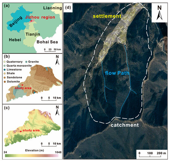
The Jizhou region, located in the northern part of Tianjin City in China, was taken as the test area. It borders Beijing to the northwest and Hebei Province to the north and east (Figure 1). The area is part of the Yanshan mountain range, which extends across northern China, and is a key transitional zone between the plain and the mountainous areas of northern China. The elevation ranges from 24 m to 1048 m ASL, with higher elevation in the north and lower in the south. The landscape is characterized by rolling hills, steep slopes, and river valleys, which play a crucial role in regional hydrological processes. Geologically, the lithology primarily consists of Proterozoic metamorphic rocks, including gneiss, schist, and quartzite (Figure 1b). Intrusive igneous rocks, such as granite and diorite, are also present in certain zones [38]. The outcropping lithologies of the investigated catchment are dolomites and dolomite limestones from the Jurassic period (J_xw), which have a layered structure and are rather weathered. The soil layers vary with elevation, geological formations, and climatic influences. Mountain brown soil, typically found in higher elevations, is well-drained with moderate organic content, making it relatively stable (https://www.resdc.cn/). Cinnamon soil, prevalent in lower hills and valleys, supports agricultural activities but is prone to erosion under heavy rainfall. Alluvial soil dominates along riverbanks and floodplains, offering nutrient conditions for vegetation but also increasing the potential for waterlogging and sediment deposition [39]. The loose and unconsolidated nature of some soil layers on steep slopes elevates the risk of landslides and debris flows, especially during rainy seasons. Regarding the climate regime, the study area experiences a temperate monsoon climate, characterized by distinct seasonal variations. Summers are hot and humid, whereas winters are cold and dry with occasional snowfall and strong northwest winds. The region receives an annual precipitation of approximately 660 mm, with the majority occurring between June and August, which commonly account for over 75% of the annual rainfall [40]. The number of days with rainfall is ~70 days on a yearly basis.

Figure 1. (a) Location of the study area; (b,c) show the lithology map and DEM of the Jizhou region, respectively, and (d) is the general overview of the Zhaojiayu (ZJY) catchment from the remote-sensing imagery.

Overall, the region is characterized by complex geomorphology conditions, consisting of mountainous terrain, river valleys, and dense human settlements. fractured and weathered rock masses, frequent human activities (e.g., slope cutting, mining, etc.), and seasonal rainfall, evidently increasing the likelihood of natural hazards. Some cases which have been reported in the literature caused severe casualties and economic losses [41], highlighting the urgent need for quantitative risk assessment of geohazards in this area.

2.2. Characteristics of the Zhaojiayu Debris Flow

The Zhaojiayu (ZJY) debris flow in the Jizhou region was taken as the test case. It was determined within the framework of a project which aimed to identify potential geohazards, coordinated by Hebei University of Technology. The coordinates of the catchment are 117°20′41″ E, 40°06′14″ N, with elevations ranging from 240 to 620 m ASL. The total area of the catchment is 1.7 km² with two main channels, and their lengths are 1.2 km and 1.0 km, respectively. The overall slope angle of the gully is approximately 36°, and the channel is relatively straight. The dominant land cover types were forests and shrubs, especially in the source and transition zones. A settlement with dense population was located at the outlet of the gully.

The ZJY is a potential hazard which has still not occurred; therefore, professional monitoring measures were not implemented before the project. We applied the SBAS-InSAR technology to obtain the surface deformation of the site. SBAS-InSAR has been widely applied to obtain the deformation time series during a given period, especially for the regions where in-suit field surveys or monitoring are difficult to perform. It yields better performance than traditional InSAR approaches, since it uses the image pair with a short spatiotemporal baseline to generate an interferogram to improve coherence [42]. The project was conducted from 2024, so SLC images of 770 Sentinel-1A acquisitions in the study area from 22 October 2014 to 16 November 2023 were acquired, with a central incidence angle of 30.66°. The image pairs were screened with a time baseline limit of 60 days and a space baseline limit of 120 m.

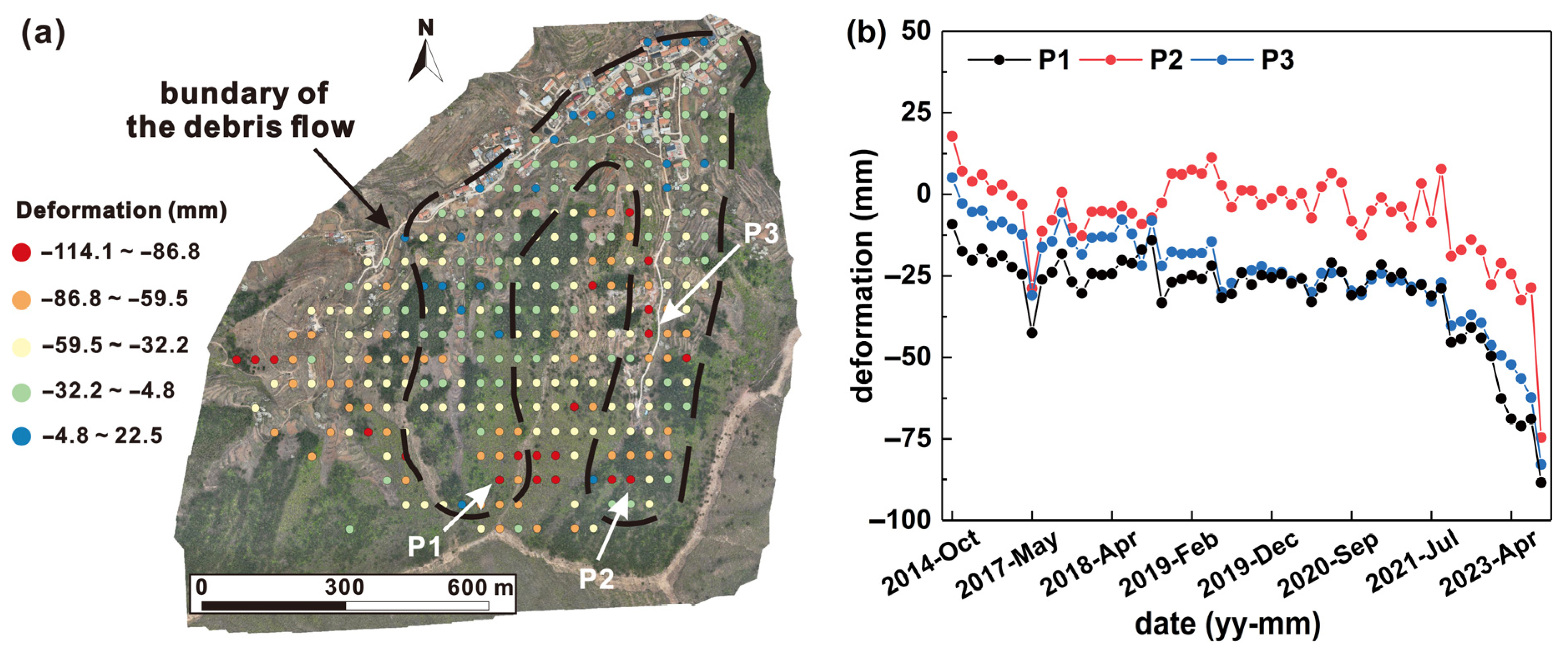
According to the spatial distribution of cumulative deformation (Figure 2), ZJY and its surrounding regions present evident deformation behavior. The overall deformation range of each monitoring point was about 100 mm. In particular, the deformation rate at specific points (P1, P2 and P3) since 2021 has become faster, reaching nearly 50 mm/year. Moreover, the deformation trend at the top of the channel was obvious, which could provide material sources for the initiation of the debris flow. In situ investigations also indicated that small-scale failures and collapses have occurred in certain areas (see Section 3.2) because of unstable Quaternary deposits. In this context, the ZJY was designated as a potential geohazard by local authorities in 2023. However, quantitative risk assessment is still necessary, since stakeholders and residents must know potential consequences when the debris flow occurs under future scenarios.

Figure 2. Distribution of the cumulative deformation of the ZJY debris flow during 2014 and 2023. (b) The monthly deformation of three points, the locations of which are presented in (a).

3. Data and Methods

3.1. Proposed Framework for Debris Flow Risk Assessment

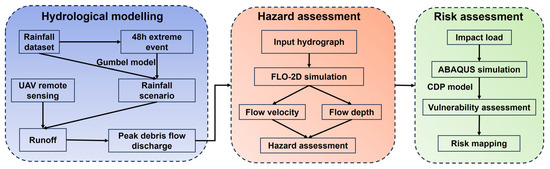
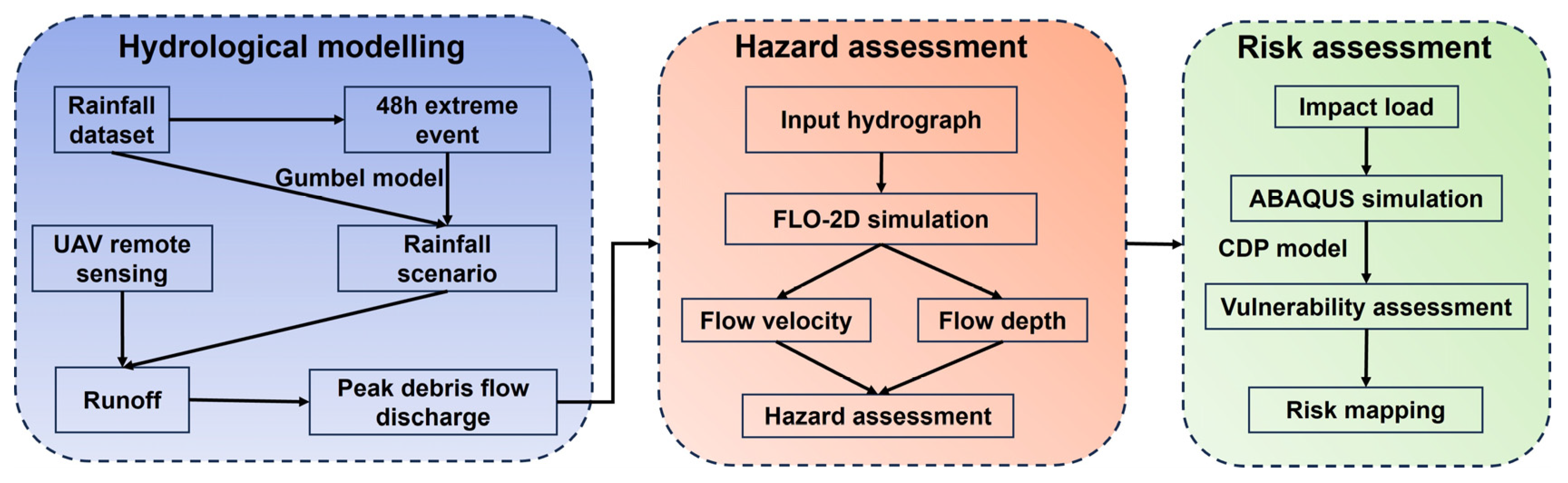
The proposed procedure mainly consists of following steps (Figure 3): We first obtained 48 h rainfall extremes based on the daily rainfall data from 1961 to 2017 and calculated the extreme rainfall under different recurrence periods through the Gumbel extreme analysis model, which was used as different rainfall scenarios in the study. Then, we conducted assessments from two aspects of hazard and vulnerability, respectively. According to different rainfall scenarios, a model was established in FLO-2D software (Basic version) to analyze the kinematic characteristics of the debris flow, including the influence range, flow velocity and flow depth. These characteristics were necessary to help understand the hazard level. It should be noted that a physically based model, the fast shallow landslide assessment model (so-called FSLAM), was utilized to compute discharge under different rainfall scenarios, since discharge was an important parameter for the simulation of debris flows.

Figure 3. The proposed methodology of this study.

For the vulnerability assessment, the threatened buildings exposed in the deposit zone of the debris flow were modeled in ABAQUS 2025. The dynamic characteristics of the debris flow were applied to determine the impact loads, and the load curve from the debris flow on the buildings over time was captured. The vulnerability of each building was quantified based on the concrete damage plasticity (CDP). Finally, the risk was determined by combining the hazard and vulnerability assessments using a judgment matrix, where the economic values for elements at risk were estimated.

3.2. UAV Remote Sensing

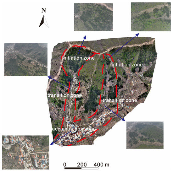
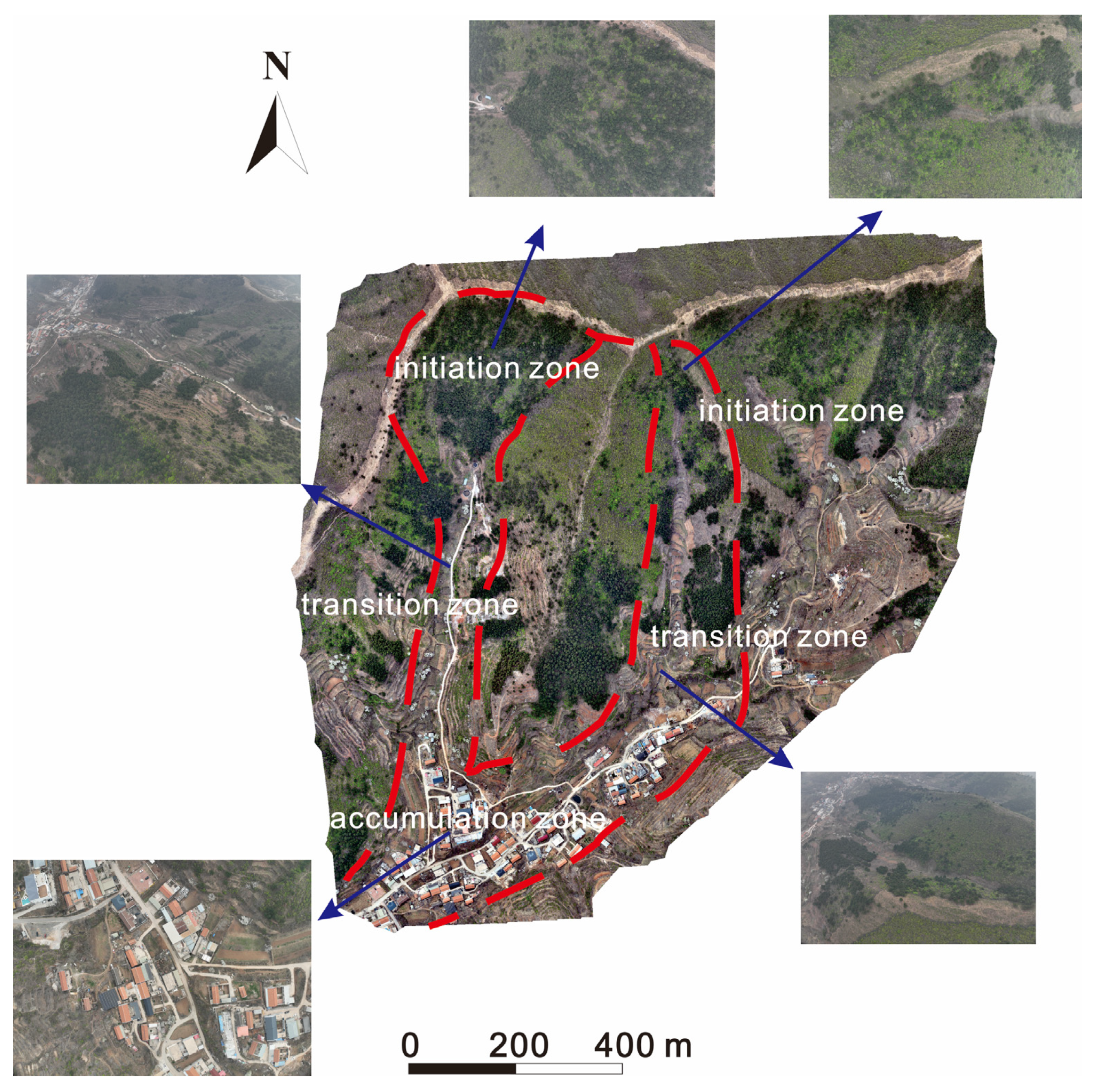
In this study, the DJI Mavic 3 drone (DJI, Shenzhen, China) was used for aerial data acquisition, since its strong endurance allowed for a long flight and an improvement of the efficiency and coverage. The drone is equipped with a three-camera system (pan, pitch, zoom), including a wide-angle camera with 20 megapixels, which supports multi-angle and multi-zoom shooting and flexibly adapts to different scenes. Next, the DJI Smart Map software v4.0.8 was applied for data processing. It provides precise route planning capabilities that help effectively cover target areas while ensuring data integrity and consistency. Regarding the flight parameters, the forward overlap rate was set to 85%, with a side overlap rate of 80%. The simulated flight altitude was set to 120 m to facilitate both orthographic and oblique photogrammetric modeling. The obtained images have high resolution with 0.08 m, which presents the overall terrain conditions (Figure 4). The two channels are clearly revealed, as well as the settlements at the outlet. Forests and farmland are the most dominant vegetation in the source and transition areas.

Figure 4. The photos obtained from the drones showing the in situ conditions of the debris flow.

3.3. Frequency Distribution Modeling for Extreme Rainfall

The rainfall frequency distribution within the study area was analyzed through extreme value statistics to determine the potential scenarios triggering landslides. A set of methods has been proposed for this purpose, such as the Gumbel distribution [43], the Weibull distribution [44], the Pearson distribution [36], etc. Considering the applicability of these methods and the available datasets in the area, the Gumbel distribution was selected to analyze the temporal probability of rainfall events exceeding a specific threshold within a given return period. Its probability density function (PDF) and cumulative density function (CDF) can be expressed as follows:

$$f\left(x\right)=\left({\displaystyle \frac{1}{\alpha }}\right)exp\left[-\left({\displaystyle \frac{x-\beta }{\alpha }}\right)-\mathrm{e}\mathrm{x}\mathrm{p}(-\left({\displaystyle \frac{x-\beta }{\alpha }}\right))\right]$$

(1)

$$F\left(x\right)=exp\left[-\mathrm{e}\mathrm{x}\mathrm{p}(-({\displaystyle \frac{x-\beta }{\alpha }})\right]$$

(2)

where β is the positional parameter of the distribution, α is the scale parameter, and the relationship between the mean parameter (μ) and these two parameters is as follows:

$$\mu =\beta +0.5772\alpha$$

(3)

Among them, α and β can be estimated by using the maximum likelihood method (MLE). The extreme rainfall (R_T) in mm with a given return period of years is determined by the following equation:

$$R_T=\mu -\alpha \left[\ln \ln ({\displaystyle \frac{T}{T-1}})\right]$$

(4)

A long-term daily rainfall dataset spanning from 1961 to 2017 at a local meteorological station was used to conduct extreme frequency modeling. Considering that a 2-day duration was the most frequent rainfall duration of the study area, the maximum rainfall for two continuous days of the year was selected as the analysis sequence. The procedure for estimating the distribution parameters with MLE was validated with the Kolmogorov–Smirnov and Anderson–Darling tests, at a confidence level of 95%. Herein, the modeling is based on a stationary assumption that the statistical characteristics of rainfall dataset do not vary with time.

3.4. Debris Flow Hazard Assessment

3.4.1. Runout Simulation Based on FLO-2D

In this study, FLO-2D software was used to simulate the runout process of the ZJY debris flow. It is a two-dimensional flood and debris flow simulation software [45], which can be applied in various fields such as disaster management, engineering risk design, urban flooding analysis, and so on. It can reasonably predict the extent of accumulation or inundation through calculations of flow velocity and accumulation depth, so as to provide support for further disaster risk zonation and the design of engineering alternatives [46].

The continuity equation and the motion equation are the basic governing equations of FLO-2D, where the volume and mass conservation of debris flow or flood are considered as follows:

$${\displaystyle \frac{\partial h}{\partial t}}+{\displaystyle \frac{\partial h{V}_x}{\partial x}}+{\displaystyle \frac{\partial h{V}_y}{\partial y}}=i$$

(5)

$$S_{fx}=S_{bx}-{\displaystyle \frac{\partial h}{\partial x}}-{\displaystyle \frac{v_x}{\mathrm{g}}}\left({\displaystyle \frac{\partial v_x}{\partial x}}\right)-{\displaystyle \frac{V_y}{\mathrm{g}}}\left({\displaystyle \frac{\partial v_x}{\partial y}}\right)-{\displaystyle \frac{1}{\mathrm{g}}}\left({\displaystyle \frac{\partial V_x}{\partial t}}\right)$$

(6)

$$S_{fx}=S_{bx}-{\displaystyle \frac{\partial h}{\partial x}}-{\displaystyle \frac{v_x}{\mathrm{g}}}\left({\displaystyle \frac{\partial v_x}{\partial x}}\right)-{\displaystyle \frac{V_y}{\mathrm{g}}}\left({\displaystyle \frac{\partial v_x}{\partial y}}\right)-{\displaystyle \frac{1}{\mathrm{g}}}\left({\displaystyle \frac{\partial V_x}{\partial t}}\right)$$

(7)

where h is the water depth, i is the rainfall intensity, t is the time, g is the gravitational acceleration, S_bx and S_by are the slope of the bottom bed in x and y direction, and S_fx and S_fy are the energy slope in x and y direction. The angular symbol x represents the momentum equation in the X-axis direction of the model and is used to represent the force balance. The dynamic wave model is mainly based on the momentum equation in the X-axis direction.

3.4.2. Hydrograph Calculation Based on Runoff Model

One important input for FLO-2D modeling is the discharge hydrograph, which is a difficult task to determine from rainfall settings [47]. For this purpose, a physically based model, namely FSLAM, is used to calculate the runoff of the channel in this study [48]. The model includes two modules, the stability and runoff modules. The former incorporates the geotechnical and hydrological models to conduct slope stability. In particular, the factor of safety is computed as follows:

$$FS={\displaystyle \frac{C}{\mathrm{g}{\rho }_{s}Z\cos \theta \sin \theta }}+\left(1-\left({\displaystyle \frac{h}{Z}}\right)\left({\displaystyle \frac{{\rho }_w}{{\rho }_s}}\right)\right)\left({\displaystyle \frac{\tan \phi }{\tan \theta }}\right)$$

(8)

where C is cohesion, g is gravity, ρ_s is saturated soil density, z is soil depth, θ is slope angle, h is groundwater level, ρ_w is water density, and φ is internal friction angle. Note that h and z are measured in the vertical direction. Cohesion is considered as the sum of two parts: one part comes from rock and soil mass C_s, and the other part comes from the apparent cohesion C_r generated by soil roots.

The most important task for the above stability calculation is to determine the value of h, which is closely related to rainfall conditions. For this step, it is necessary to consider both groundwater table changes caused by antecedent rainfall and extreme rainfall events. In detail, the former provides the initial condition for the landslide and commonly occurs on a mid- to long-term timescale. The corresponding groundwater level increase (h_a) can be expressed by following [49]:

$$h_a=\left({\displaystyle \frac{a}{b}}\right){\displaystyle \frac{q_a}{K\sin \theta \cos \theta }}\left({\displaystyle \frac{{\rho }_w}{{\rho }_s}}\right)$$

(9)

where a is the drainage area, b is the cell size, q_a is the effective antecedent recharge, and K is the horizontal hydraulic conductivity. The event rainfall infiltration corresponds to the vertical flow in the short-term, and it causes groundwater water level variation (h_e) according to:

$$h_e={\displaystyle \frac{P_e}{n}}-{\displaystyle \frac{{\left(p_e-\left(5080/CN-51\right)\right)}^2}{n·\left(P_e+4·\left(5080/CN-51\right)\right)}}$$

(10)

where P_e is event rainfall which represents the boundary condition for landslides. n is soil porosity and CN is the curve number proposed in the event oriented SCS-CN model, which is a hydrological model. It is an empirical parameter for predicting direct runoff or infiltration from rainfall excess, only related to the runoff threshold and the soil water storage. In addition, to address the uncertainty of soil properties, a stochastic model has been proposed to allow the input parameters to have a statistical distribution over a range of possible values. Hence, both the factor of safety and the probability of failure can be output from the model.

For a given rainfall scenario, the infiltration is related to discharge in the channel, which is subsequently determined by the runoff module. The procedure is conducted across the study area, and the spatial distribution of peak discharge at each pixel for different extreme rainfall can be derived. The curve number is the only parameter required at this stage. Specifically, the calculation of runoff in FSLAM applies the rational method that requires the tributary area, the rainfall intensity and the runoff coefficient. The runoff coefficient (C) is determined using the following equation [4]:

$$C={\displaystyle \frac{\left(P_e-I_a\right)·\left(P_e+23I_a\right)}{{\left(P_e+11I_a\right)}^2}}$$

(11)

where I_a is the initial abstraction computed from CN. Then, the rainfall intensity is computed using the Intensity–Duration–Frequency (IDF) curves:

$$I=I_{d}11\left({\displaystyle \frac{{28}^{0.1}-{T_c}^{0.1}}{{28}^{0.1}-1}}\right)$$

(12)

where I is the rainfall intensity, I_d is the daily rainfall intensity measured as millimeters per hour, and T_c is the concentration time of the catchment.

Next, according to the Specification of Geological Investigations of Debris Flow Stabilization in China [50], the peak debris flow discharge (Q_c) can be adjusted from the peak water discharge by following [51]:

$$Q_c=\left(1+\varnothing \right)·Q_p·D_c$$

(13)

where Q_p is the peak runoff calculated from the FSLAM model, D_c is the obstructive coefficient of the debris flow ranging from 1.5 to 2.5, ∅ is correction factor, and it can be denoted as following:

$$\varnothing =\left({\gamma }_c-{\gamma }_w\right)/\left({\gamma }_h-{\gamma }_c\right)$$

(14)

where γ_c is the total unit weight of the debris flow, γ_w is the unit weight of water, γ_h is the unit weight of solid materials. Subsequently, a generalized pentagon method is adopted to generate the input hydrograph [50]. Since long-term monitoring is unavailable in this case, the empirical method is used. Notably, the so-called generalized hydrograph is summarized by extensive engineering practices in China and has been widely applied. It sets the debris flow discharge as Q_c/4 at T/3 and Q_c/3 at 2T/3 (T is the total simulation time). Combined with the start (Q = 0), middle (Q = Q_c) and end moment (Q = 0), the input hydrograph was determined using a cubic spline interpolation.

Next, a QGIS plugin was used for FSLAM modeling in this study, which allows for the implementation of the model automatically [52]. It requires five raster files as inputs, namely DEM, soil type, LULC, q_a and P_e. DEM was obtained from UAV mapping with an original resolution of 0.1 m. LULC and soil type were collected as a shapefile form originally from the Chinese Academy of Sciences (https://www.resdc.cn/), which were subsequently transformed into raster files. According to the archived report of local authority, the average level of antecedent rainfall (q_a) was around 0.4 mm/d and the P_e is the calculated result from extreme value distribution. It should be noted that q_a and P_e are constant across the area for a specific scenario. All these input files were transformed into 3m resolution to ensure the same coordinate system and spatial extent.

3.5. Vulnerability Assessment of Elements at Risks

The ABAQUS software v4.0.8 was applied to simulate the deformation of buildings under impacts from the debris flow. It is a widely used finite element analysis software which can simulate the mechanical behavior of various engineering materials and structures. Since the volume of potential sources of the ZJY debris flow is relatively small, the components of the materials were considered relatively uniform with small stone sizes. Under this context, the impact load on structures can be assumed to take the form of a rectangular pulse that is divided into two categories [32,53]: one is the impact load due to kinematic process, and the other is the accumulation load when the movement stops. The former is determined as follows:

$$P_{dy}=\lambda \rho {{\upsilon }_c}^2\sin \alpha$$

(15)

where ρ_dy is the average impact load, unit N/m²; V_c is the motion velocity vector; λ is the shape factor of the buildings and infrastructures in which 1.0 is used for circular buildings and 1.33 for rectangle buildings, and α is the angle between the stress surface of the building and the impact pressure direction. The accumulation load can be denoted as following:

$$P_{st}={\displaystyle \frac{\rho \mathrm{g}\mathrm{h}}{2}}$$

(16)

where ρ is the average density of materials; g is gravity; h is the accumulation depth of debris flow.

The velocity and depth simulated from FLO-2D analysis can be used to obtain the total impact load at a given location, and the load curves on buildings versus time. The load is subsequently used as the input in ABAQUS to capture the dynamic responses of buildings, including displacement, von Mises stress, tension and compression damage, and stiffness degradation of concrete. Considering the failure of reinforced concrete (RC) frame structures is mainly attributed to the degradation of material stiffness [54], we mainly apply this indicator to characterize the vulnerability of buildings. Specifically, we focus on the stiffness failure situations of primary load-bearing components and count the number of grids (N) that have stiffness degradation at different moments. Herein, the analysis of secondary load-bearing components is not included in order to quantify this synergistic effect among different elements. Hence, the ratio between N and the total number of grids (M), defined as P_i (i is the time), represents the damage degree of the component. Next, the vulnerability (V) at a given moment can be determined as follows:

$$V={\displaystyle \frac{P_i}{P_{i,max}}}$$

(17)

where P_i,max is the first mutation point on the P_i curve versus time, since it is considered that the structure has been destroyed; namely, the vulnerability is 1.

3.6. Quantitative Risk Assessment

Within the framework of the quantitative risk assessment of natural hazards, the risk (R) is characterized and quantified by the product of hazard (H), vulnerability (V) and the economic value (E) of the elements at risk [55]. In this study, we also adopt this widely used principle to calculate the risk as follows:

$$R=H\times V\times E$$

(18)

For the ZJY debris flow, the flow velocity and depth derived from numerical simulation are considered to characterize the hazard. A heuristic matrix is used to combine the two indicators to determine the hazard level (Table 1). It should be noted that hazard assessments commonly include both spatial and temporal probabilities [56]. Given that complete disaster catalog and recurrence records are not available in the study area, the real annual probability fails to be obtained for the ZJY debris flow. Therefore, the temporal probability of the triggering factors (mainly rainfall) is used to characterize the temporal probability of the debris flow. In addition, the value of vulnerability should first be determined for the affected structures according to the kinematic characteristics of the debris flow. For the buildings located in the deposit areas, the procedure described in Section 3.5 is used to quantify the damage and vulnerability. For infrastructures other than buildings, vulnerability is determined mainly based on qualitative empirical knowledge.

Table 1. The heuristic matrix to determine hazard level used in this study.

	Height (m)	h < 0.5	0.5 ≤ h < 1.5	h > 1.5
Velocity (m/s)
v < 0.5		Low	Medium	High
0.5 ≤ v < 1.5		Medium	High	Very high
v > 1.5		High	Very high	Very high

Finally, through the risk matrix, we combine the hazard, vulnerability and the value of buildings to complete the quantitative risk assessment under different rainfall scenarios [57,58,59].

4. Results

4.1. Hazards Assessment Under Extreme Rainfall

4.1.1. Variation in Peak Discharge and Hydrology

As seen in Table 2, the extreme rainfall with different return periods is 183.0 mm, 213.3 m and 235.2 mm, respectively. They are used as the event rainfall for the FSLAM model and the calculated peak discharge in the channel is 2.4 m³/s, 2.9 m³/s and 3.2 m³/s. According to the descriptions in Section 3.4.2, the discharge is adjusted by the coefficient to obtain the peak value of the hydrograph, namely 40.8 m³/s, 49.3 m³/s and 54.4 m³/s, respectively.

Table 2. Extreme rainfall and corresponding peak discharge under different scenarios.

	Scenario	p = 5% (RT = 20a)	p = 2% (RT = 50a)	p = 1% (RT = 100a)
Output
Extreme rainfall (mm)		183.0	213.3	235.2
Peak discharge (m3/s)		2.4	2.9	3.2
Peak hydrograph (m3/s)		40.8	49.3	54.4

4.1.2. Kinematic Characteristics of the Debris Flow

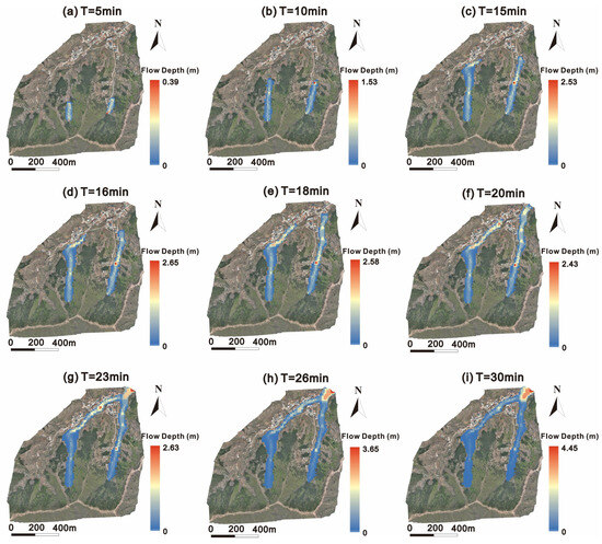
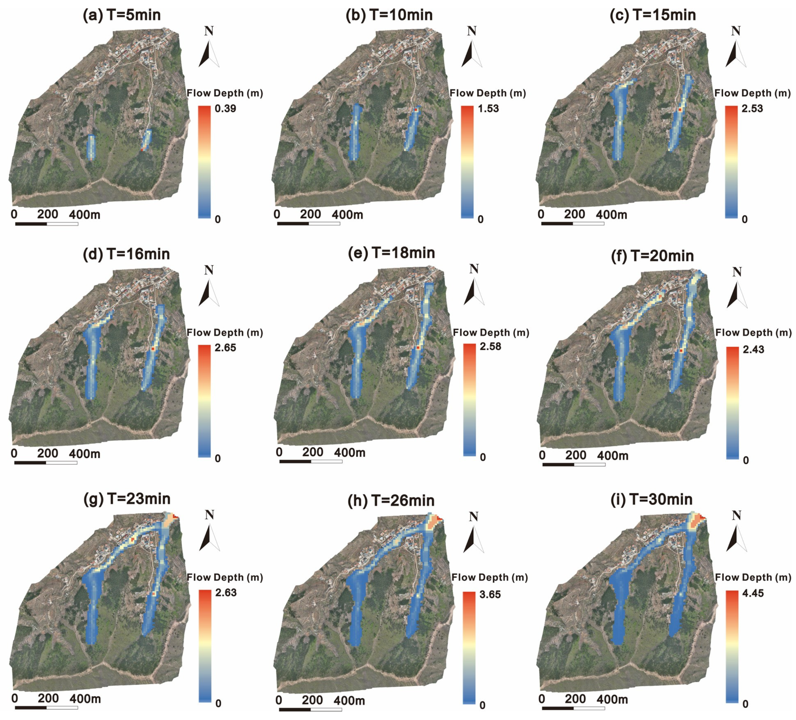
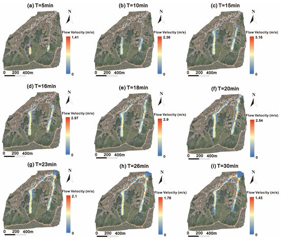
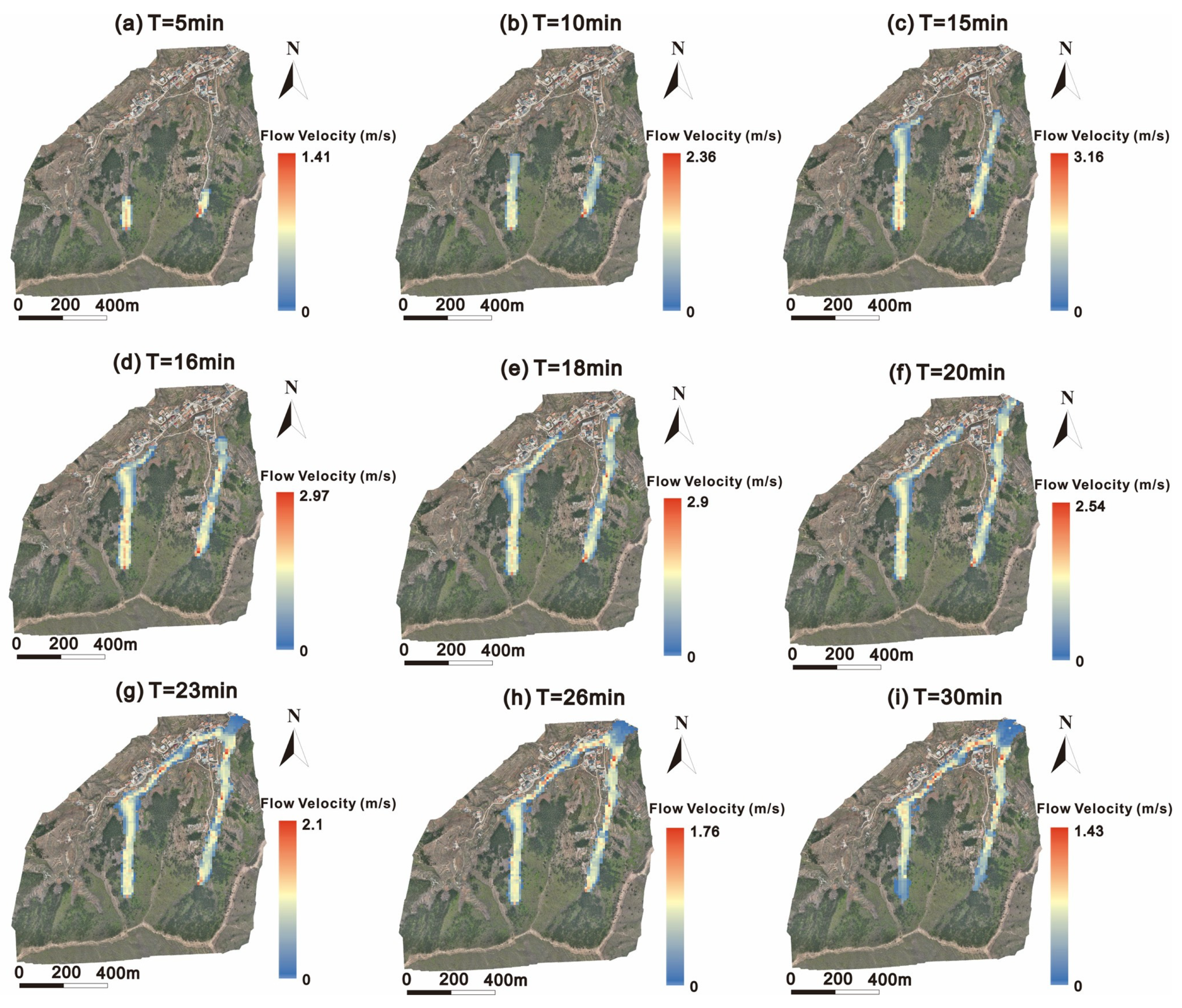
The parameters for the movement simulation of the ZJY debris flow are shown in Table 3. Due to the limited space, herein only the scenario of the 50-year return period rainfall is used as an example to show the kinematic characteristics from initiation to stopping. Initially, the materials begin to develop at two different gullies as the discharge increases, and local siltation in the relatively flat areas of the gully is observed (Figure 5). The largest accumulation depths in the two gullies are 2.4 m and 2.2, respectively. By T = 23 min, the two flows merge at the densely populated village at the channel outlet, reaching a maximum depth of 4.5 m. Regarding the flow velocity (Figure 6), the movement of the debris flow becomes faster from the beginning to T = 15 min. After that, the velocities are lower due to the curving of the channel and blocking of the buildings at the toe of the gully. Most materials are deposited at the village, with most velocities lower than 1 m/s at T = 30 min.

Table 3. The parameters used in the FLO-2D simulation.

Sediment Specific Gravity	Volume Concentration	Manning Coefficient	Viscosity		Yield Stress		Laminar Flow Resistance
			α1	β1	α2	β2
2.5 × 103 kg/m3	55%	0.1	0.811	13.72	0.00462	11.24	2280

Figure 5. The depth distribution at different moments of the ZJY debris flow under the rainfall with p = 2%.

Figure 6. The flow velocity distribution at different moments of the ZJY debris flow under the rainfall with p = 2%.

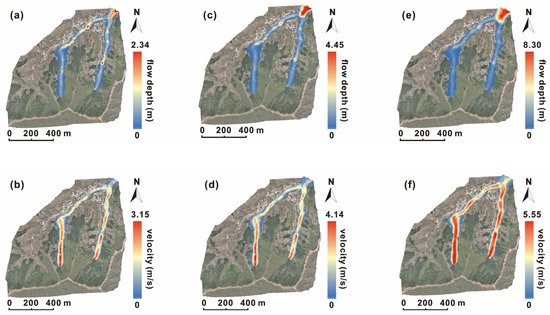
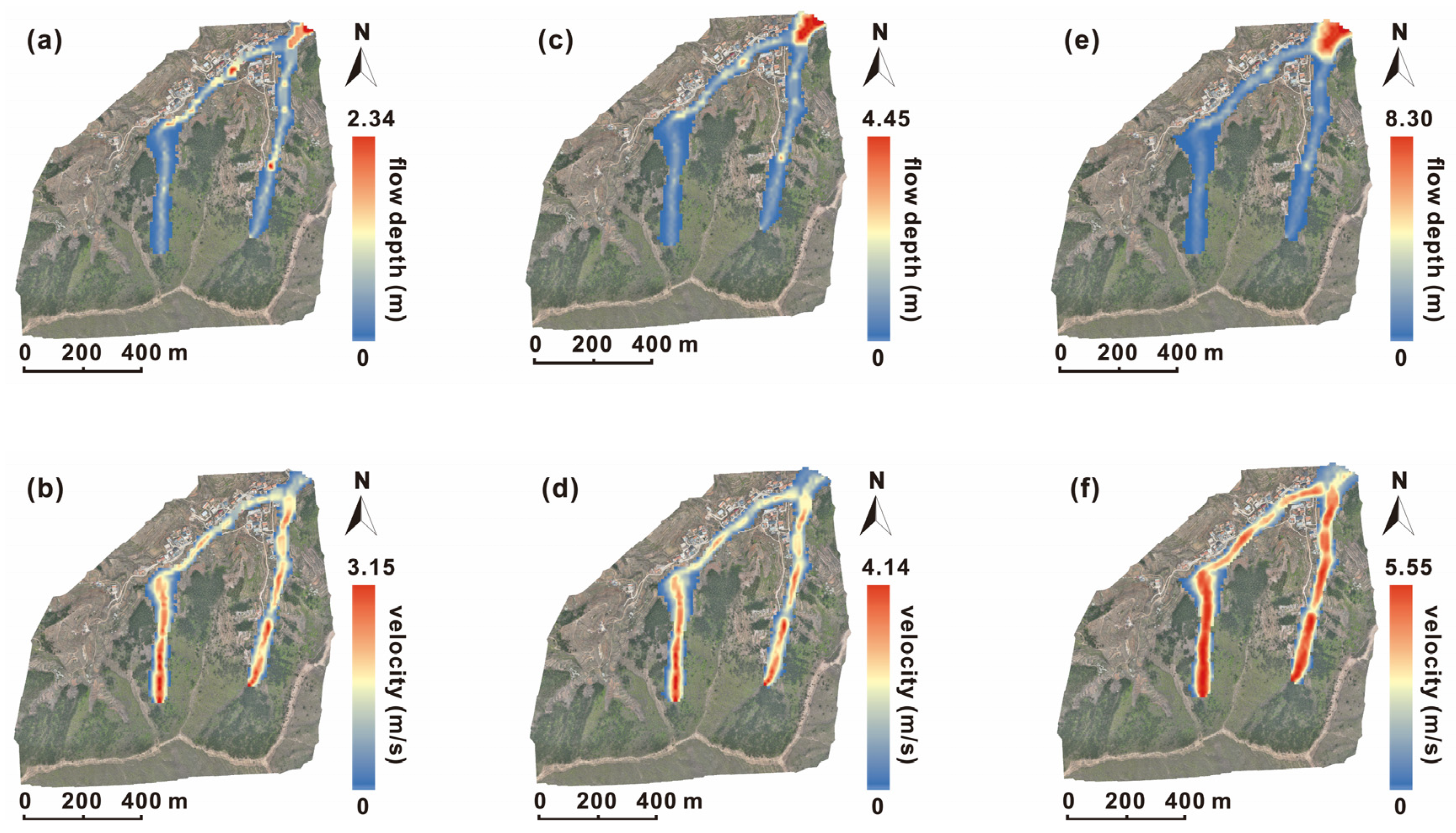
Next, the maximum flow depth and velocity for different scenarios are analyzed (Figure 7). Under the 20-year return period rainfall, the maximum deposit depth mainly concentrates at the gully outlet which reaches 2.34 m. The larger velocities are observed in the narrow and straight channel, especially in its upper section (source area), with a peak of 3.15 m/s. In addition, the left channel has a larger average velocity than the other channel. The velocity gradually decreases at the toe of the gully where materials are deposited, evidently leading to larger accumulation depth in the village area than that of source and transit zones. When the rainfall frequency increases to 2%, the deposit zones at the gully outlet significantly expand, and most areas have depths higher than 2 m. The maximum deposit depth reaches up to 4.45 m. The highest velocity increases by 31.7% compared with the previous scenario. When it comes to the rainfall with the 100-year return period, the sediment accumulation in the gully is smaller, as most of the materials are transported to the flat terrain downstream. The maximum deposit reaches 8.3 m, whereas the peak velocity reaches to 5.55 m. It should be noted that the average velocity in the channel in this scenario is evidently larger than that of the other scenarios.

Figure 7. (a) The maximum flow depth in 20-year return period rainfall, (b) The maximum flow velocity in 20-year return period rainfall, (c) The maximum flow depth in 50-year return period rainfall, (d) The maximum flow velocity in 50-year return period rainfall, (e) The maximum flow depth in 100-year return period rainfall, (f) The maximum flow velocity in 100-year return period rainfall.

Overall, the outlet of the gully and the village always experience the largest deposit depth among all the scenarios, whereas peak velocity is observed in the channels. Although there is not too much difference among the peak hydrographs, the flow depth and velocity distribution show evidently different magnitudes. For example, the maximum depth increases by 90.2% (from 2.34 m to 4.45 m) and 86.5% (from 4.45 m to 8.3 m), respectively.

4.2. Vulnerability Assessment

4.2.1. Vulnerability Calculation from ABAQUS Simulation

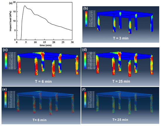
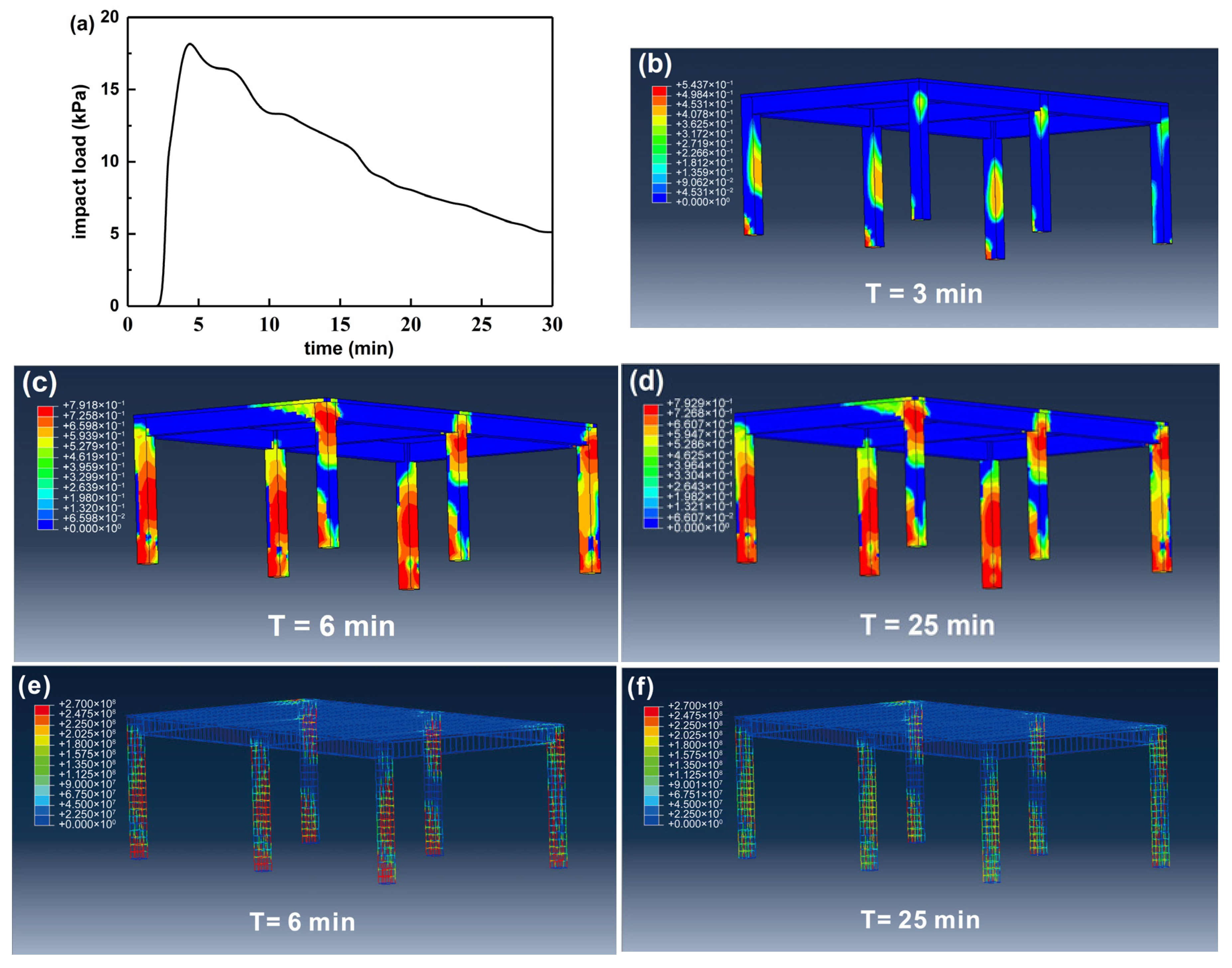
Considering the number of affected buildings, a single building with an RC frame structure located at the outlet of the gully is taken as an example (see Figure 1 for its location) to analyze the progressive damage of the building. Based on the results of flow depth and velocity at the building, the impact load curve on the structure is obtained (Figure 8a). The results show that the debris flow reaches the building at 2.7 min. Subsequently, the impact pressure rapidly increases with a peak of 19.3 kPa at 4.2 min. However, the dynamic pressure decreases significantly after that due to the dissipation of the materials’ kinetic energy. When the debris flow stops, the pressure remains at 5.1 kPa, which is attributed to the deposit accumulation.

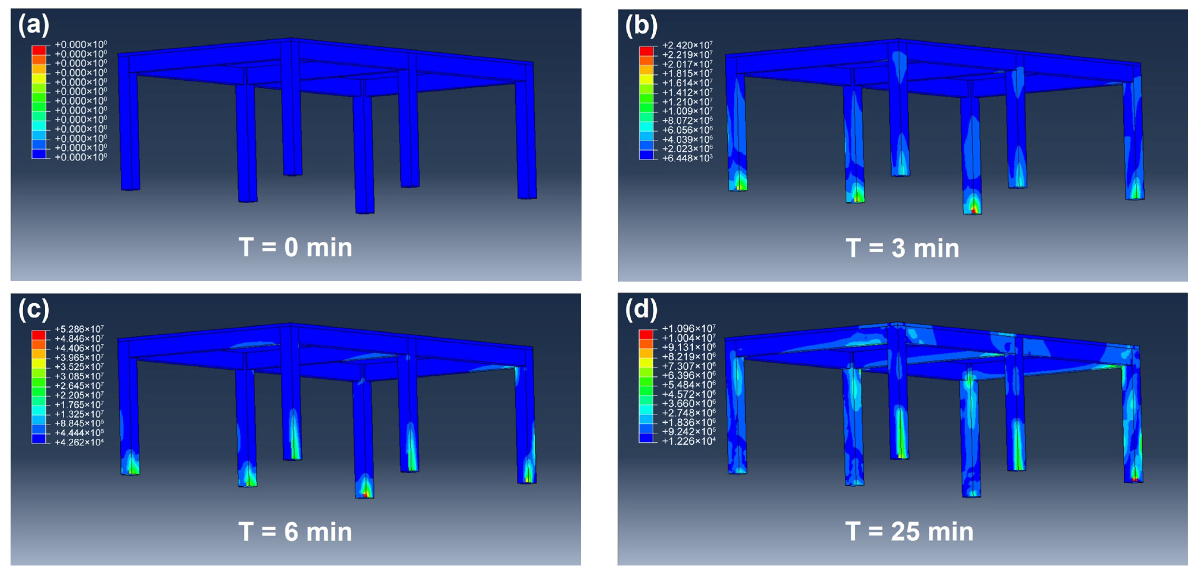
Figure 8. (a) The impact load curve on the structure for ABAQUS simulation. (b–d) show the concrete Mises stress of the structure at different moments (T = 3 min, 6 min, 25 min). (e,f) show the reinforcement stress at T = 6 min and T = 25 min.

From the stress distribution versus time (Figure 8b–d), with the increase in impact load, the maximum external force on the structure is always located at the corner column of the impacted side. The maximum stress value is 5.3 × 10⁷ Pa occurring at 6 min, after which the stress gradually decreases and finally stabilizes at 6.4 × 10⁶ Pa. This is consistent with the variation in the impact load curve. In addition, we note a large stress at the beam–column connection in the middle section of the unimpacted side. This is mainly because of the rigid connection at this part, which limits the displacement of the column more than that of the side column. Next, the reinforcement stress of the building is also analyzed (Figure 8e,f). It can be seen that the location where the maximum stress occurs is similar to that of concrete. The maximum value reaches 2.7 × 10⁸ Pa at T = 6 min. After that, although the impact load gradually decreases, the stress of the reinforcement still remains around this value and extends along the direction away from the longitudinal reinforcement. This indicates that external concretes has failed during this phase whereas the reinforcement becomes the primary load-bearing component. By comparing the stress of the concrete and steel bars at the same moment, we find that the latter remains approximately ten times the former.

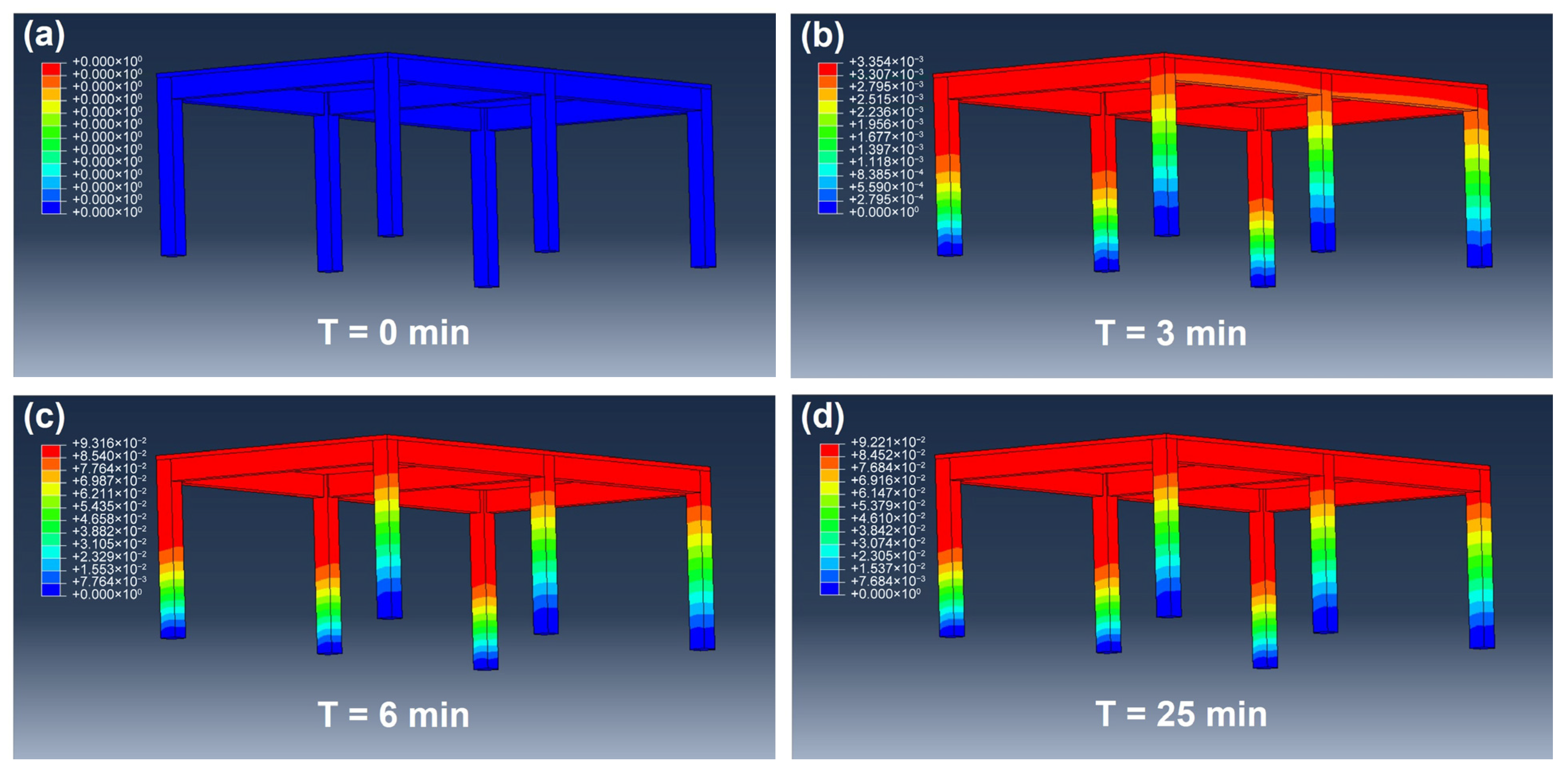
Regarding the structural displacement results (Figure 9), they gradually increase with the impact load at the initial phase. However, the displacement still increases after the impact load reaches the peak at T = 6 min, thus indicating the deformation of the structure lags behind the impact from the debris flow. After T = 15 min, the displacement shows elastic rebound behavior, and final displacement stabilizes at 0.335 mm. Compared with the largest displacement, the rebound magnitude is 0.1 mm. This revealed that concrete had a self-recovery capability following plastic damage, and the current impact magnitude was insufficient to cause a complete failure of the structure.

Figure 9. The total displacement of the structure at different moments: (a) T = 0 min, (b) T = 3 min, (c) T = 6 min, (d) T = 25 min.

From the concrete damage of the building (Figure 10), the concrete of the six side columns has stiffness degradation of different degrees. For the columns that face to the impact, the damaged section appears on the inside part, and spreads continuously in the first 6 min. This is because this section is mainly the tension area. In the following 6–30 min, the protective layer of concrete fails with the increase in load and the deformation of steel bars also increases. This coincides with the extension of the stress of the steel bar mentioned above. Moreover, the damaged zone on the side which does not face the impact load appears at the joint between the bottom and the top of the column and the beam. This is because more boundary constraints occur at these sections with the increase in displacement, resulting in stress concentration in the concrete under tension. Next, the number of grids in the concrete damaged area after a sudden increase is counted, and the building vulnerability is determined at 0.73 by comparing with the total number of grids in the model.

Figure 10. Concrete damage cloud map of the changes with time: (a) T = 0 min, (b) T = 3 min, (c) T = 6 min, (d) T =25 min.

4.2.2. Vulnerability Mapping

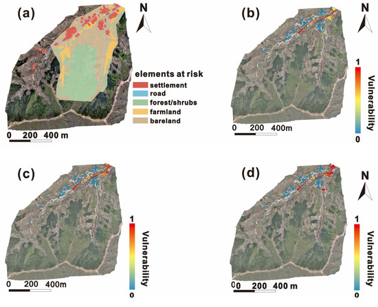
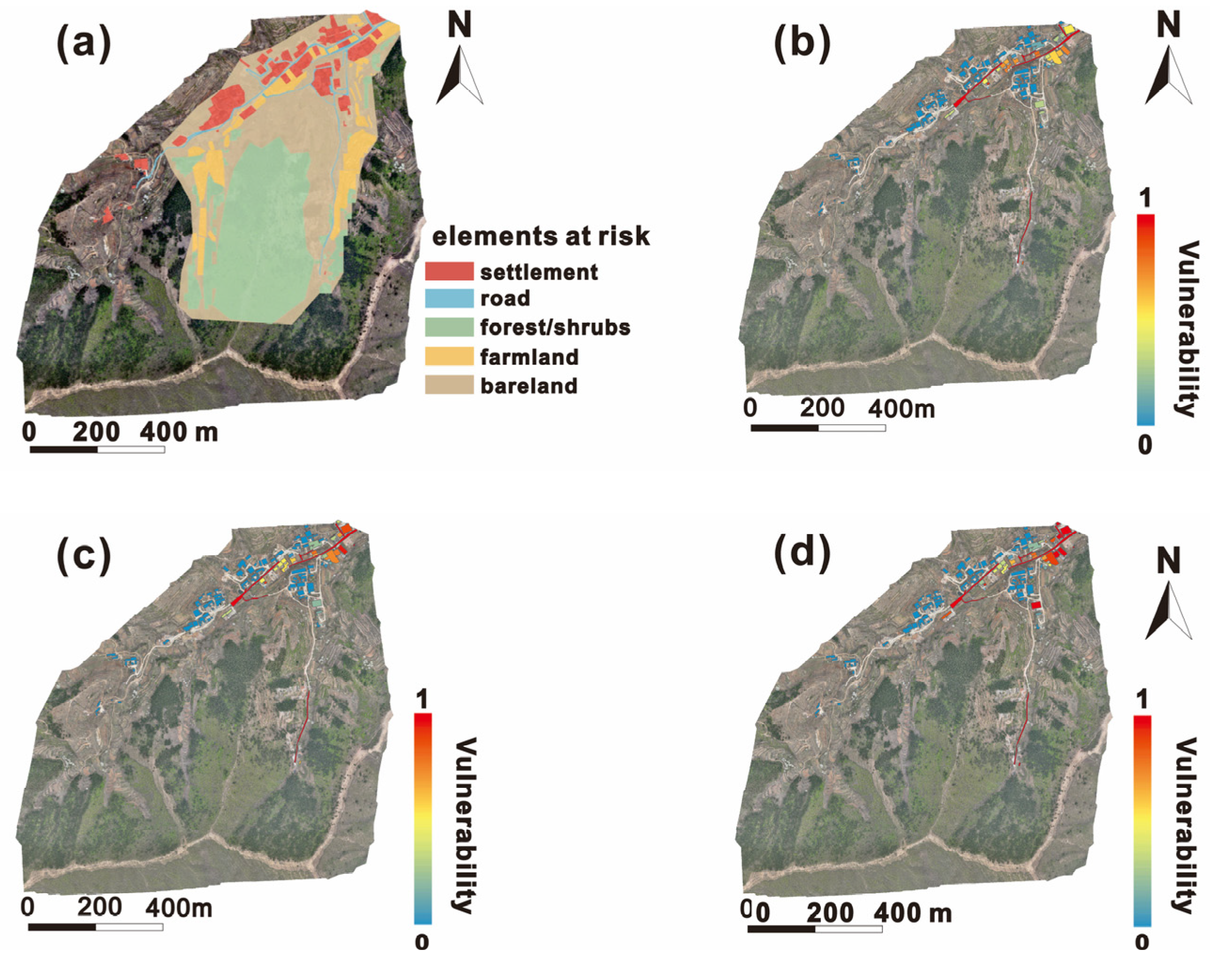
Based on the UAV remote sensing and visual interpretation results, all buildings and infrastructures within the affected area of the debris flow are identified and visualized. As seen in Figure 11, the types of elements at risk mainly include residential areas, transportation facilities (mainly roads), woodland, farmland, and bare land. Next, the vulnerability of each building is also obtained by following the same analysis procedure described in Section 4.2.1. ArcGIS software v10.2 is used to assign and visualize the vulnerability values of the elements at risk to generate vulnerability maps.

Figure 11. The results of vulnerability assessment for buildings and infrastructures. (a) The classification of elements at risks. (b–d) show the vulnerability of buildings and roads under different scenarios, including 20-year return period rainfall (b), 50-year return period rainfall (c), and 100-year return period rainfall (d).

We observe that the areas with high vulnerability are always concentrated in the gully outlet and deposit zone. With the increase in the rainfall and the deposition of debris flow materials, the overall vulnerability of buildings also increases. The proportion of buildings with very high and high vulnerability rises from 30.7% (20-year return period) to 41.2% (100-year return period), and the number of threatened people also increases from ~100 to ~150.

4.3. Scenario-Based Quantitative Risk Assessment

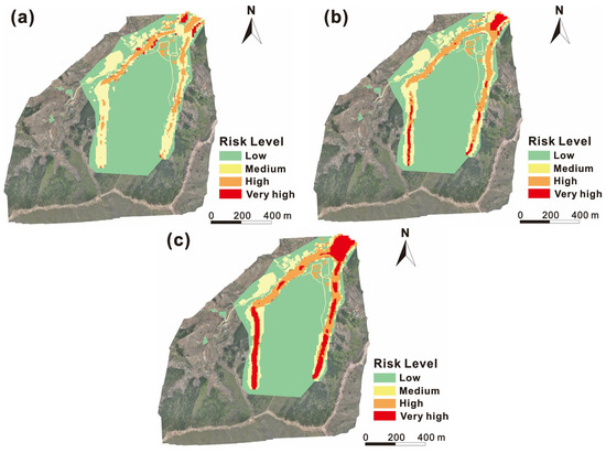
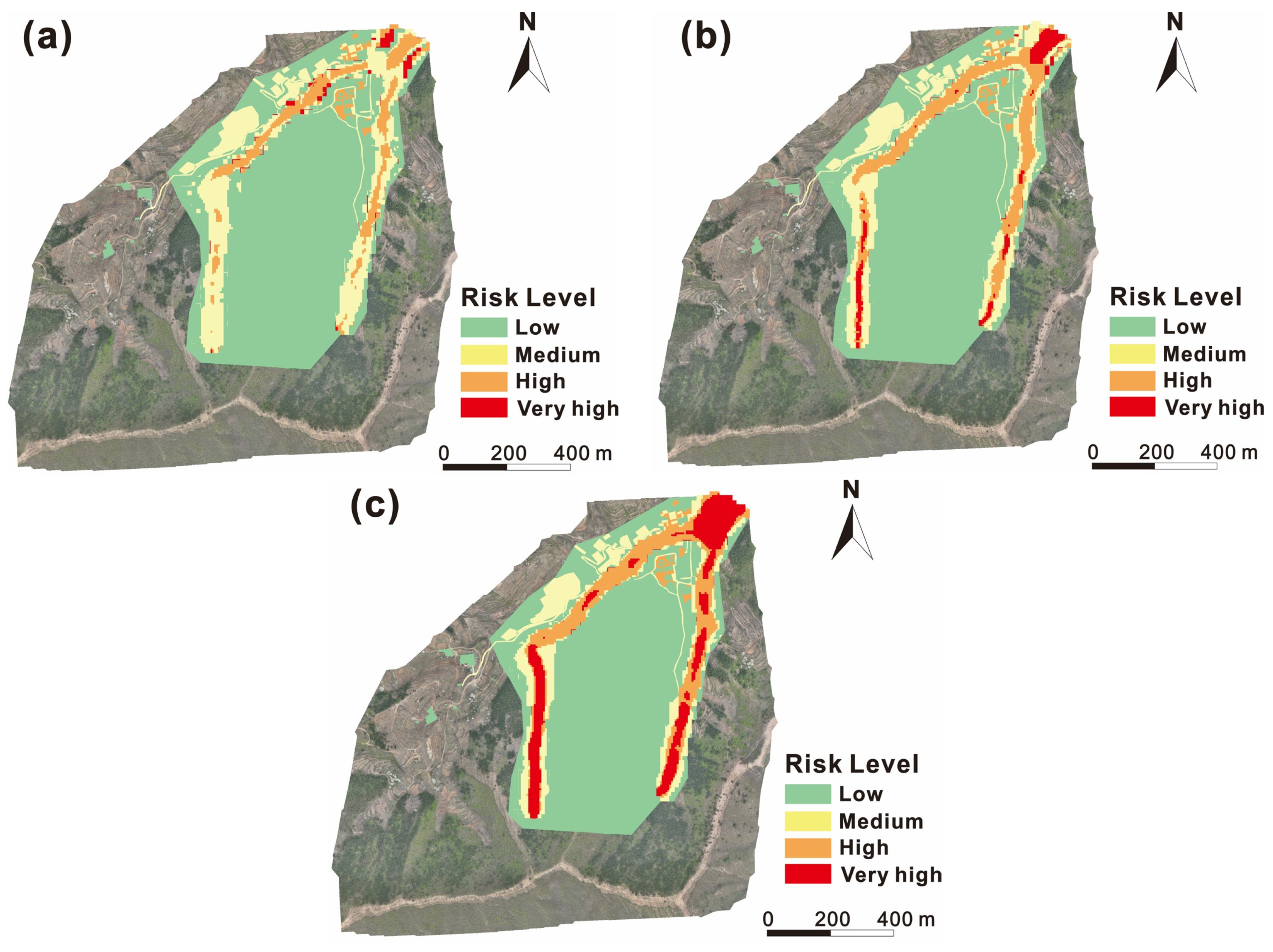
The risk results under different scenarios are shown in Figure 12. From the overview of the spatial distribution, zones with very high or high risk levels are mainly located along the road in the village and the intersections of the two channels. It should be noted that high-risk zones increase significantly when it comes to the rainfall scenarios with 50-year and 100-year return periods compared to that in 20-year return period rainfall. In particular, the risk level of most areas in the channels becomes very high risk. Given that there are no buildings located in the channels, the flow velocity and depth (namely the debris flow hazard) are the most important affecting the variation in risk. In detail, the total proportion of very high- and high-risk zones reaches 19% (20-year R_T), 26% (50-year R_T), and 31% (100-year R_T), respectively. Hence, the risk values increase with the return period of rainfall.

Figure 12. (a) is the risk level map at p = 5%, (b) is the risk level map at p = 2%, and (c) is the risk level map at p = 1%.

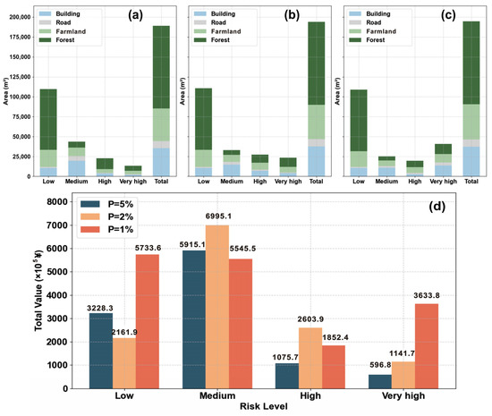
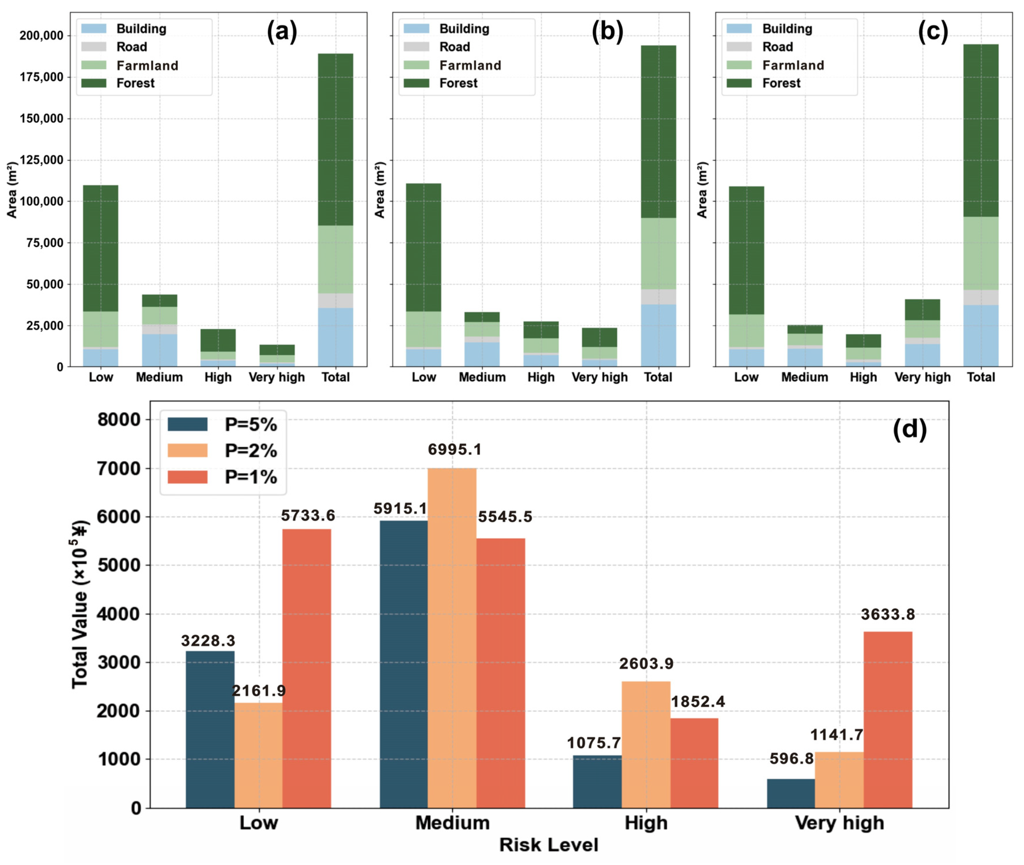
In addition, the risk level distribution for different elements at risk is also analyzed (Figure 13a–c). Spatially, the largest areas of high-risk zones are located on forest and agricultural lands, where no residents live or are threatened. However, a higher proportion of buildings and roads in very high-risk zones is also observed as the rainfall increases, which certainly poses higher risks to residents. Hence, residents and infrastructures affected by the debris flow should be focused on under extreme rainfall. Next, the economic loss of elements at risk is quantified based on current market pricing and costs (Figure 13d). Under the 20-year return period rainfall scenario, the economic losses are mainly reported in the low- and medium-risk zones, with a value of approximately ¥108.1 million. When the return period rises up to 50 years, the proportion of medium-risk zones remains large, but the economic losses of high-risk and very high-risk zones increase significantly. When RT = 100a, the economic losses of high risk and very high risk become ¥167.7 million. In particular, the total economic risk in very high-risk level is 6.1 times that for 20-year return period rainfall.

Figure 13. The risk distribution in different types of elements at risk under the (a) 20-year return period, (b) 50-year return period, (c) 100-year return period. (d) shows the economic risks for different risk levels under different scenarios.

5. Discussion

A key aspect of the current study is determining the hydrology during debris flow events, which is related to rainfall intensity and accumulation [60,61]. This study uses the FSLAM model to calculate peak discharge and adjusts it to obtain the input hydrology by using an empirical coefficient. The volume concentration (C_v) is not applied like in some other studies [62], which introduces uncertainties. However, it should be noted that the ZJY debris flow is an event that has not occurred yet, so the instability volume is difficult to quantify to determine C_v under variable rainfall conditions. Despite this, the runoff model considers the topography, vegetation and antecedent conditions, which may affect the infiltration and discharge behavior [13]. Hence, it is considered to improve the reliability of triggering condition settings compared with typical methods such as empirical discharge estimates [63] and semi-distributed models [32]. Particularly, the procedure provides a possibility for the calibration of different parameters that are used in FSLAM modeling.

After the determination of peak discharge, a generalized pentagon method is adopted to generate the input hydrograph for the ZJY debris flow, which has been widely used for FLO-2D simulation but is not accurate enough. However, it should be mentioned that both the empirical (including this study) and simulation methods (e.g., NAM and HEC-HMS models) may generate errors regarding the runoff [32]. In this context, the computed results must be verified or calibrated by the continuous monitoring of data; however, it is not commonly available for mountainous areas [13]. In addition, many debris flow events occur suddenly and cannot be foreseen, so it is unrealistic to implement monitoring in advance. In particular, this study aims to analyze the potential debris flow, and it is more difficult to determine its accurate triggering scenarios. This is not only an issue in this study, but also in many other studies. For example, Chang et al. [64] also used a generalized curve to generate the input hydrology for a debris flow that already occurred in southwest China. Notably, the so-called generalized pentagon method is not just an imaging method, but an approach based on extensive engineering practices, especially in China. It is recommended by local [65] and national specifications in China [50] and once yielded good performance [66]. In addition, the uncertainty during this step can also be attributed to the processing of rainfall data. Specifically, the total duration of the event is set to 30 min, but the considered rainfall condition is on a daily basis. We fail to determine the local rainfall distribution or intensity during the event, since the duration of the debris flow from initiation to stopping is difficult to determine. It can be found that the set durations varied considerably with case studies, from several minutes [67] to over ten hours [47]. The rainfall data with high resolution (within minute) is not available in this study (actually also the case in most studies), so we assigned the daily rainfall obtained from the extreme value modeling to the 30 min duration. It is a simplification, but this coincides with the rainfall regime in rainy seasons in the northern and eastern China; namely, extreme rainfall events normally occur over a short term (several minutes to several hours) and account for the majority of daily rainfall [68,69]. Hence, the 30 min duration was considered acceptable. Certainly, this may overestimate the results of runoff and debris hazard. Hence, a technique that generates a debris flow discharge hydrograph from the given runoff (or rainfall conditions) and catchment terrain may be of high interest in the future. In fact, some methods on this topic have been proposed [70], but they normally require sufficient in situ monitoring data or local characteristics. In addition, high-resolution precipitation data, which is typically derived from satellite remote sensing, is also a potential solution [71]. It can improve spatial analysis capabilities but remains challenging for applications in mountainous terrains due to scale mismatches and measurement errors.

Another source of uncertainty is associated with the stationarity of rainfall time series. The rainfall frequency modeling in this study is based on the stationary assumption that the statistical characteristics of the rainfall dataset do not vary with time. However, the change in the Earth’s climate system is unequivocal, so both the abundance and the magnitude of extreme rainfall events are expected to be different under future climate scenarios [3]. However, the changing trends are still not clear and may depend largely on local meteorological conditions and climate regimes. For instance, Wasko et al. [72] reported that extreme rainfall has increased, with greater increases for more extreme events, by examining trends in streamflow events using over 2000 monitoring stations worldwide. On the contrary, Zhai et al. [73] found downward trends in total rainfall and extreme rainfall in north China between 1951 and 2000. Hence, it is necessary to inform users about this potential impact, but the details can be determined only through scientific and systematic analysis, which is not the main objective of the present study. We find that some studies have attempted to integrate climate model outputs into probabilistic debris flow predictions [74], but uncertainties in climate predictions and scaling methods affect the reliability of results. Furthermore, the temporal clustering of debris flows, namely the rapid and consecutive occurrence of multiple events, makes risk assessments more complicated. In this context, it is necessary to develop a dynamic model that accounts for temporal dependencies and evolving system sensitivity [75]. For this purpose, nonstationary time series and dynamic parameters for frequency distribution should be incorporated into the analysis in future works.

Regarding the vulnerability assessment of buildings, we analyze the dynamic response by using ABAQUS, where the dynamic characteristics of the debris flow from FLO-2D simulation are used to compute impact loads on structures. The uncertainties of this process have multiple origins, among which the geotechnical parameters of the FLO-2D should be stated. Given that sufficient soil samples were not collected, these parameters are determined according to expert experience and the standard literature [45]. However, additional but limited laboratory tests for the in situ soil samples show that the sediment-specific gravity was from 2.36 × 10³ kg/m³ to 2.71 × 10³ kg/m³, whereas the range for laminar flow resistance was from 2210 to 2560. It is evident that our settings coincide with these results. Regarding the other parameters, namely viscosity and yield stress, it is hard to directly measure them. We compare them with the literature (e.g., [47]), which reviewed and compiled the parameters used in previous works worldwide. It is found that the values for α₁ (0.811), α₂ (0.00462), β₁ (13.72), β₂ (11.24) used in our manuscript fit well with previous studies. In particular, the used values are close to the mode reported in these studies, which further validates the reliability of the present study. Nevertheless, empirical studies have shown that variations in input parameters can induce uncertainties in debris flow simulations [76]. Hence, the cross-validation with empirical data and the standard literature can only reduce the uncertainty rather than eliminate it. On the other hand, it should be noted that FLO-2D only allows deterministic values for input parameters. However, the spatial–temporal variation in geotechnical parameters naturally exists. Evidently, the uncertainty from soil parameterization is an inherent issue in debris flow simulation. Hence, it is important to admit it and conduct sensitivity analyses of parameters in future works.

Second, a minor uncertainty is associated with the adoption of stiffness degradation of concrete. Given that most studies used it only for assessing the damage behavior of buildings, this study is an uncommon attempt to apply it to characterize building vulnerability. However, ABAQUS also provides some other indicators as outputs (e.g., drift ratios, residual stiffness), which can be used for further cross-validation to obtain the complete interpretation. Notably, the reasonableness of using other indicators to quantify building vulnerability should be further validated, since few studies have addressed this topic, unlike stiffness degradation. In addition, a few recent studies indicate that the damage of structures should consider the function of various components, including both primary and secondary load-bearing components [77]. However, it is an operational challenge to quantify this synergistic effect among different elements, especially when it comes to the numerical simulation methods. Hence, this study still focuses on the load-bearing components, since they control the damage behavior of buildings. In addition, computational efficiency is also a concern, since the statistics for all components are evidently time-consuming even when using the automatic tool in ABAQUS.

Last but not least, as Corominas et al. [20] concluded, each link of quantitative risk assessment is inevitably fraught with uncertainties. The most significant contribution of the present study is proposing a quantitative framework for debris flow risk assessment. The validation procedure is indeed absent, but this does not affect the flexibility of the proposed methodology. For example, the methodology can be replicated in any mountainous setting to generate quantitative landslide risk maps, as soon as the typography, rainfall and infrastructure data is available. The implementation of the whole procedure will not be changed by the absence of detailed validation. We also note that the main outputs of the present study coincide with those from other regions [3,5,37], thus indicating reliability and generalizability. This means its theoretical foundations are considered robust, and it can be expected that it will be better understood and adapted once more events are used as case studies. In addition, remote sensing mapping has demonstrated its advantages through this case, especially regarding the identifications and investigations of potential hazards. Previous works [51,66] using traditional field measurements were normally time-consuming, and essentially back-analyses rather than predictions. It is evident that the InSAR and UAV techniques have wide applications for engineers and planners who should respond promptly to geo-disasters.

6. Conclusions

Extreme rainfall events have been more frequent due to global climate change, but standardized methods for risk assessment posed by natural hazards are still lacking. In particular, vulnerability assessment is commonly considered a weak component within the framework of risk assessment. The present study proposes a quantitative procedure to assess rainfall-induced debris flow risk and demonstrates its application by using a case study (the Zhaojiayu debris flow) in northern China. Our analysis reveals the following three main outcomes:

(i)

Differences among the peak discharges in the channel generated from extreme rainfall scenarios are not evident, which are 2.4 m³/s (R_T = 20a), 2.9 m³/s (R_T = 50a), and 3.2 m³/s (R_T = 100a), respectively. However, the overall flow velocity and deposit depth show a visible increase in the simulation results of FLO-2D.

(ii)

The ABAQUS analysis manages to simulate the dynamic response and progressive damage of buildings. We use the stiffness degradation of concrete as the indicator for structure vulnerability and generate the vulnerability maps for different scenarios. The zones with higher vulnerability concentrate in the gully outlet and deposit zone. The proportion of buildings with very high and high vulnerability rises from 30.7% (20-year return period) to 41.2% (100-year return period).

(iii)

Forest and farmland account for most of the very high-level risk zones, but a higher proportion of buildings and roads in very high-risk zones is observed as rainfall increases, which certainly poses higher risks to residents. The obtained total economic risk of the debris flow reaches ¥167.7 million when it comes to the 100-year return period rainfall scenario, increasing by 55.1% compared with that of the 20-year return period rainfall scenario.

Overall, the current analysis highlights the importance of identifying and quantitatively predicting the risk of natural hazards that have not occurred yet, rather than conducting back-analysis regarding historical events. The proposed method is promising for improving the accuracy of hazard and vulnerability mapping by incorporating multiple numerical schemes. Given that the risk level for residents and infrastructures will considerably increase with the change in extreme rainfall, risk reduction alternatives may be necessary for the Zhaojiayu debris flow in the future.

References

- Eidsvig, U.M.K.; Kristensen, K.; Vangelsten, B.V. Assessing the risk posed by natural hazards to infrastructures. Nat. Hazards Earth Syst. Sci. 2017, 17, 481–504. [Google Scholar] [CrossRef] [Scilit]
- Criss, R.E.; Stein, E.M. A Cost-Effective Flood Warning System for Small Urban Basins. J. Earth Sci. 2025, 36, 307–313. [Google Scholar] [CrossRef] [Scilit]
- Mishra, A.N.; Maraun, D.; Knevels, R.; Truhetz, H.; Brenning, A.; Proske, H. Climate change amplified the 2009 extreme landslide event in Austria. Clim. Change 2023, 176, 124. [Google Scholar] [CrossRef] [Scilit]
- Hürlimann, M.; Guo, Z.; Puig-Polo, C.; Medina, V. Impacts of future climate and land cover changes on landslide susceptibility: Regional scale modelling in the Val d’Aran region (Pyrenees, Spain). Landslides 2022, 19, 99–118. [Google Scholar] [CrossRef] [Scilit]
- Stanley, T.A.; Soobitsky, R.B.; Amatya, P.M.; Kirschbaum, D.B. Landslide Hazard Is Projected to Increase Across High Mountain Asia. Earth’s Future 2024, 12, e2023EF004325. [Google Scholar] [CrossRef] [Scilit]
- Keck, J.; Istanbulluoglu, E.; Strauch, R.; Cristea, N. Could Climate Change Decrease Landslide Hazard in Snow-Dominated Mountainous Regions? Insights From a Distributed Hydrology-Shallow Landslide Model of the North Cascades, USA. Water Resour. Res. 2025, 61, e2025WR040071. [Google Scholar] [CrossRef] [Scilit]
- Gariano, S.L.; Guzzetti, F. Landslides in a changing climate. Earth-Sci. Rev. 2016, 162, 227–252. [Google Scholar] [CrossRef] [Scilit]
- Guo, Z.; Zeng, T.; Zhang, Y.; Yu, W.; Wang, L.; Guo, Z.; Glade, T. A novel hybrid model integrating high resolution remote sensing and stacking ensemble techniques for landslide susceptibility mapping: Application to event-based landslide inventory. Geomorphology 2025, 486, 109886. [Google Scholar] [CrossRef] [Scilit]
- Kim, H.G.; Park, C.; Cho, M. Finding unrevealed landslide hazard area induced by climate change and topography—Case study for Inje-Gun, Gangwon-Do, ROK. Sustain. Cities Soc. 2021, 75, 103180. [Google Scholar] [CrossRef] [Scilit]
- Feng, P.; Li, C.; Zhang, S.; Meng, J.; Long, J. Integrating shipborne images with multichannel deep learning for landslide detection. J. Earth Sci. 2024, 35, 296–300. [Google Scholar] [CrossRef] [Scilit]
- Zheng, X.; Lu, W.; Jiang, R.; Li, J.; Zhang, L. Analysis of landslide on Meizhou-Dapu expressway based on satellite remote sensing. Geoenviron. Disasters 2025, 12, 25. [Google Scholar] [CrossRef] [Scilit]
- Hungr, O.; Leroueil, S.; Picarelli, L. The Varnes classification of landslide types, an update. Landslides 2014, 11, 167–194. [Google Scholar] [CrossRef] [Scilit]
- Guo, X.; Li, Y.; Chen, X.; Zhang, J.; Sun, Y. Variation of debris flow/flood formation conditions at the watershed scale in the Wenchuan Earthquake area. Landslides 2021, 18, 2427–2443. [Google Scholar] [CrossRef] [Scilit]
- van Vuuren, D.P.; Edmonds, J.; Kainuma, M.; Riahi, K.; Thomson, A.; Hibbard, K.; Hurtt, G.C.; Kram, T.; Krey, V.; Lamarque, J.-F.; et al. The representative concentration pathways: An overview. Clim. Change 2011, 109, 5. [Google Scholar] [CrossRef] [Scilit]
- Kim, H.; Kim, T.; Shin, J.Y.; Heo, J.H. Improvement of Extreme Value Modeling for Extreme Rainfall Using Large-Scale Climate Modes and Considering Model Uncertainty. Water 2022, 14, 478. [Google Scholar] [CrossRef] [Scilit]
- Acero, F.J.; García, J.A.; Gallego, M.C. Peaks-over-threshold study of trends in extreme rainfall over the Iberian Peninsula. J. Clim. 2011, 24, 1089–1105. [Google Scholar] [CrossRef] [Scilit]
- Guo, Z.; Chen, L.; Gui, L.; Du, J.; Yin, K.; Do, H.M. Landslide displacement prediction based on variational mode decomposition and WA-GWO-BP model. Landslides 2020, 17, 567–583. [Google Scholar] [CrossRef] [Scilit]
- Zou, Q.; Cui, P.; He, J.; Lei, Y.; Li, S. Regional risk assessment of debris flows in China—An HRU-based approach. Geomorphology 2019, 340, 84–102. [Google Scholar] [CrossRef] [Scilit]
- Xiao, L.; Wang, J.; Zhu, Y.; Zhang, J. Quantitative risk analysis of a rainfall-induced complex landslide in Wanzhou County, Three Gorges Reservoir, China. Int. J. Disaster Risk Sci. 2020, 11, 347–363. [Google Scholar] [CrossRef] [Scilit]
- Corominas, J.; van Westen, C.; Frattini, P.; Cascini, L.; Malet, J.-P.; Fotopoulou, S.; Catani, F.; Van Den Eeckhaut, M.; Mavrouli, O.; Agliardi, F.; et al. Recommendations for the quantitative analysis of landslide risk. Bull. Eng. Geol. Environ. 2014, 73, 209–263. [Google Scholar] [CrossRef] [Scilit]
- Guo, Z.; Cheng, M.; Wang, Y.; Xu, G.; Zhang, Y.; Xu, C. Landslide hazard prediction under extreme rainfall scenario by considering multiple timescale rainfall and effective recharge. Georisk 2025, 17, 740–754. [Google Scholar] [CrossRef] [Scilit]
- Iverson, R.M. The physics of debris flows. Rev. Geophys. 1997, 35, 245–296. [Google Scholar] [CrossRef] [Scilit]
- Li, Y.; Xu, L.; Shang, Y.; Chen, S. Debris flow susceptibility evaluation in Meizoseismal Region: A Case Study in Jiuzhaigou, China. J. Earth Sci. 2024, 35, 263–279. [Google Scholar] [CrossRef] [Scilit]
- Zhou, G.G.D.; Du, J.; Song, D.; Choi, C.E.; Hu, H.S.; Jiang, C. Numerical study of granular debris flow run-up against slit dams by discrete element method. Landslides 2020, 17, 585–595. [Google Scholar] [CrossRef] [Scilit]
- Christen, M.; Kowalski, J.; Bartelt, P. RAMMS: Numerical simulation of dense snow avalanches in three-dimensional terrain. Cold Reg. Sci. Technol. 2010, 63, 1–14. [Google Scholar] [CrossRef] [Scilit]
- Mubarak, N.; Kumar, P.; Kumar, R.; Jakka, R.S. Physics-based modeling of debris flows and assessing the performance of effective mitigation measures. Geoenviron. Disasters 2024, 11, 34. [Google Scholar] [CrossRef] [Scilit]
- Córdoba, G.; Villarosa, G.; Sheridan, M.; Viramonte, J.; Beigt, D.; Salmuni, G. Secondary lahar hazard assessment for villa la angostura, argentina, using two-phase-titan modelling code during 2011 cordón caulle eruption. Nat. Hazards Earth Syst. Sci. 2015, 15, 757–766. [Google Scholar] [CrossRef] [Scilit]
- Leonardi, A.; Wittel, F.K.; Mendoza, M.; Vetter, R.; Herrmann, H.J. Particle–fluid–structure interaction for debris flow impact on flexible barriers. Comput.-Aided Civ. Infrastruct. Eng. 2016, 31, 323–333. [Google Scholar] [CrossRef] [Scilit]
- Bilal, M.; Kumar, R. Physical modelling to map the rheological and morphological dynamics along with entrainment mechanics of debris flow: A comprehensive review of the state of the art. Geoenviron. Disasters 2025, 12, 45. [Google Scholar] [CrossRef] [Scilit]
- Fell, R.; Corominas, J.; Bonnard, C.; Cascini, L.; Leroi, E.; Savage, W.Z. Guidelines for landslide susceptibility, hazard and risk zoning for land-use planning. Eng. Geol. 2008, 102, 99–111. [Google Scholar] [CrossRef] [Scilit]
- Fuchs, S.; Heiss, K.; Hübl, J. Towards an empirical vulnerability function for use in debris flow risk assessment. Nat. Hazards Earth Syst. Sci. 2007, 7, 495–506. [Google Scholar] [CrossRef] [Scilit]
- Wang, T.; Yin, K.; Li, Y.; Chen, L.; Xiao, C.; Zhu, H.; van Westen, C. Physical vulnerability curve construction and quantitative risk assessment of a typhoon-triggered debris flow via numerical simulation: A case study of Zhejiang Province, SE China. Landslides 2024, 21, 1333–1352. [Google Scholar] [CrossRef] [Scilit]
- Zhang, Z.; Feng, F.; Wang, T.; Dou, X. Numerical estimation of landslide runout flow–structure interactions: A case study of Zhengjiamo landslide. Bull. Eng. Geol. Environ. 2024, 83, 212. [Google Scholar] [CrossRef] [Scilit]
- Xing, L.; Wang, G.; Gong, W.; Xu, M.; Jaboyedoff, M.; Wang, F. Model tests of the failure behaviors of buildings under the impact of granular flow. Landslides 2025, 22, 373–392. [Google Scholar] [CrossRef] [Scilit]
- Shao, C.; Wang, Y.; Jia, Y.; Liang, F.; Pei, C.; Guan, P.; Jiao, Y. A Whole-Process Data Processing Method for Tunnel Seismic Geological Prediction Ahead of Tunnel Faces. J. Earth Sci. 2025, 36, 333–338. [Google Scholar] [CrossRef] [Scilit]
- Guo, Z.; Chen, L.; Yin, K.; Shrestha, D.P.; Zhang, L. Quantitative risk assessment of slow-moving landslides from the viewpoint of decision-making: A case study of the three gorges reservoir in China. Eng. Geol. 2020, 273, 105667. [Google Scholar] [CrossRef] [Scilit]
- Liu, X.; Wang, Y. Quantifying impacts of precipitation scenarios projected under climate change on annual probability of rainfall-induced landslides at a specific slope. Comput. Geotech. 2024, 167, 106063. [Google Scholar] [CrossRef] [Scilit]
- Wu, Y.X.; Lyu, H.M.; Shen, J.S.; Arulrajah, A. Geological and hydrogeological environment in Tianjin with potential geohazards and groundwater control during excavation. Environ. Earth Sci. 2018, 77, 392. [Google Scholar] [CrossRef] [Scilit]
- Liu, F.; Zhang, G.; Song, X.; Li, D.; Zhao, Y.; Yang, J.; Wu, H.; Yang, F. High-resolution and three-dimensional mapping of soil texture of China. Geoderma 2020, 361, 114061. [Google Scholar] [CrossRef] [Scilit]
- Si, P.; Li, Q.X.; Chen, X.Y.; Wang, M.; Luo, C.J. Construction of daily precipitation series and the observational characteristics of extreme precipitation in Tianjin, China during 1888–2022. Adv. Clim. Change Res. 2024, 15, 52–61. [Google Scholar] [CrossRef] [Scilit]
- Xie, F.; Wang, Z.; Liu, J. Seismic hazard and risk assessments for Beijing–Tianjin–Tangshan, China, Area. Pure Appl. Geophys. 2011, 168, 731–738. [Google Scholar] [CrossRef] [Scilit]
- Zeng, T.; Wu, L.; Hayakawa, Y.S.; Yin, K.; Gui, L.; Jin, B.; Guo, Z.; Peduto, D. Advanced integration of ensemble learning and MT-InSAR for enhanced slow-moving landslide susceptibility zoning. Eng. Geol. 2024, 331, 107436. [Google Scholar] [CrossRef] [Scilit]
- Osei, M.A.; Amekudzi, L.K.; Omari-Sasu, A.Y.; Yamba, E.I.; Quansah, E.; Aryee, J.N.A.; Preko, K. Estimation of the return periods of maxima rainfall and floods at the Pra River Catchment, Ghana, West Africa using the Gumbel extreme value theory. Heliyon 2021, 7, e06980. [Google Scholar] [CrossRef] [Scilit] [PubMed]
- Amponsah, W.; Dallan, E.; Nikolopoulos, E.I.; Marra, F. Climatic and altitudinal controls on rainfall extremes and their temporal changes in data-sparse tropical regions. J. Hydrol. 2022, 612, 128090. [Google Scholar] [CrossRef] [Scilit]
- O’Brien, J.S. FLO-2D Users Manual; FLO-2D Software, Inc.: Nutrioso, AZ, USA, 2009. [Google Scholar]
- Erena, S.H.; Worku, H.; De Paola, F. Flood hazard mapping using FLO-2D and local management strategies of dire Dawa City, Ethiopia. J. Hydrol. Reg. Stud. 2018, 19, 224–239. [Google Scholar] [CrossRef] [Scilit]
- Zeng, P.; Chen, J.; Chang, M.; Sun, X.; Li, T. Uncertainty characterization, propagation, and evaluation in debris flow run-out hazard assessment. Landslides 2025, 22, 1275–1290. [Google Scholar] [CrossRef] [Scilit]
- Medina, V.; Hürlimann, M.; Guo, Z.; Lloret, A.; Vaunat, J. Fast physically-based model for rainfall-induced landslide susceptibility assessment at regional scale. Catena 2021, 201, 105213. [Google Scholar] [CrossRef] [Scilit]
- Montgomery, D.R.; Dietrich, W.E. A physically based model for the topographic control on shallow landsliding. Water Resour. Res. 1994, 30, 1153–1171. [Google Scholar] [CrossRef] [Scilit]
- Ministry of Land and Resources (MLR), People’s Republic of China. Specification of Geological Investigation for Debris Flow Stabilization. 2006. Available online: http://www.nrsis.org.cn/mnr_kfs/file/read/55806d6159b7d8e10a42c8762c8aa99f (accessed on 10 August 2025). (In Chinese)
- Xu, Q.; Zhang, S.; Li, W.; van Asch, T.W.J. The 13 August 2010 catastrophic debris flows after the 2008 Wenchuan earthquake, China. Nat. Hazards Earth Syst. Sci. 2012, 12, 201–216. [Google Scholar] [CrossRef] [Scilit]
- Guo, Z.; Torra, O.; Hürlimann, M.; Medina, V.; Puig-Polo, C. FSLAM: A QGIS plugin for fast regional susceptibility assessment of rainfall-induced landslides. Environ. Model. Softw. 2022, 150, 105354. [Google Scholar] [CrossRef] [Scilit]
- Ghanem, A.; Lee, Y.-J.; Moon, D.-S. Seismic vulnerability of reinforced concrete frame structures: Obtaining plan or vertical mass irregularity from structure use change. J. Struct. Eng. 2024, 150, 4023243. [Google Scholar] [CrossRef] [Scilit]
- Zhuang, Y.; Ji, X.; Sun, L.; Kajiwara, K.; Kang, J.D.; Nagae, T. Damage inference and residual capacity assessment for an E-Defense 2018 ten-story RC test structure. Eng. Struct. 2024, 302, 117317. [Google Scholar] [CrossRef] [Scilit]
- Varnes, D.J. Landslide Hazard Zonation: A Review of Principles and Practice; UNESCO Natural Hazard Series; United Nations Educational, Scientific and Cultural Organization (UNESCO): Paris, France, 1984; 63p. [Google Scholar]
- Guzzetti, F.; Carrara, A.; Cardinali, M.; Reichenbach, P. Landslide hazard evaluation: A review of current techniques and their application in a multi-scale study, Central Italy. Geomorphology 1999, 31, 181–216. [Google Scholar] [CrossRef] [Scilit]
- Raetzo, H.; Lateltin, O.; Bollinger, D.; Tripet, J. Hazard assessment in Switzerland—Codes of practice for mass movements. Bull. Eng. Geol. Environ. 2002, 61, 263–268. [Google Scholar]
- Corominas, J.; Copons, R.; Vilaplana, J.M.; Altimir, J.; Amigó, J. Integrated landslide susceptibility analysis and hazard assessment in the principality of Andorra. Nat. Hazards 2003, 30, 421–435. [Google Scholar] [CrossRef] [Scilit]
- Hürlimann, M.; Copons, R.; Altimir, J. Detailed debris flow hazard assessment in Andorra: A multidisciplinary approach. Geomorphology 2006, 78, 359–372. [Google Scholar] [CrossRef] [Scilit]
- Sun, Y.; Zhang, J.; Wang, H.; Lu, D. Probabilistic thresholds for regional rainfall induced landslides. Comput. Geotech. 2024, 166, 106040. [Google Scholar] [CrossRef] [Scilit]
- Zhao, Y.; Li, Y.; Zheng, J.; Wang, Y.; Meng, X.; Yue, D.; Guo, F.; Chen, G.; Qi, T.; Zhang, Y. A new rainfall intensity−duration threshold curve for debris flows using comprehensive rainfall intensity. Eng. Geol. 2025, 347, 107949. [Google Scholar] [CrossRef] [Scilit]
- Chen, J.C.; Chuang, M.R. Discharge of landslide-induced debris flows: Case studies of Typhoon Morakot in southern Taiwan. Nat. Hazards Earth Syst. Sci. 2014, 14, 1719–1730. [Google Scholar] [CrossRef] [Scilit]
- Rickenmann, D. Empirical Relationships for Debris Flows. Nat. Hazards 1999, 19, 47–77. [Google Scholar] [CrossRef] [Scilit]
- Chang, M.; Tang, C.; Van Asch, T.W.J.; Cai, F. Hazard assessment of debris flows in the Wenchuan earthquake-stricken area, South West China. Landslides 2017, 14, 1783–1792. [Google Scholar] [CrossRef] [Scilit]
- Shen, Y.M.; Chen, T.L.; Xiao, G.J.; Fu, Q.Y.; Qing, Z.Z.; Li, L.P.; Xu, Z.C.; Leng, L.; Dong, Z.Q.; Xie, M.H.; et al. Flood Calculation Manual of Small Watershed in Sichuan Province, China; Sichuan Provincial Department of Water Resources and Electric Power: Sichuan, China, 1984. (In Chinese) [Google Scholar]
- Chen, M.; Tang, C.; Zhang, X.; Xiong, J.; Chang, M.; Shi, Q.; Wang, F.; Li, M. Quantitative assessment of physical fragility of buildings to the debris flow on 20 August 2019 in the Cutou gully, Wenchuan, southwestern China. Eng. Geol. 2021, 293, 106319. [Google Scholar] [CrossRef] [Scilit]
- Badoux, A.; Graf, C.; Rhyner, J.; Kuntner, R.; McArdell, B.W. A debris-flow alarm system for the Alpine Illgraben catchment: Design and performance. Nat. Hazards 2009, 49, 517–539. [Google Scholar] [CrossRef] [Scilit]
- Gu, X.; Ye, L.; Xin, Q.; Zhang, C.; Zeng, F.; Nerantzaki, S.D.; Papalexiou, S.M. Extreme Precipitation in China: A Review on Statistical Methods and Applications. Adv. Water Resour. 2022, 163, 104144. [Google Scholar] [CrossRef] [Scilit]
- Yin, J.; Li, F.; Li, M.; Xia, R.; Bao, X.; Sun, J.; Liang, X. The unique features in the 4 d widespread extreme rainfall event over North China in July 2023. Nat. Hazards Earth Syst. Sci. 2025, 25, 1719–1735. [Google Scholar] [CrossRef] [Scilit]
- Li, Y.; Meng, X.; Guo, P.; Dijkstra, T.; Zhao, Y.; Chen, G.; Yue, D. Constructing rainfall thresholds for debris flow initiation based on critical discharge and S-hydrograph. Eng. Geol. 2021, 280, 105962. [Google Scholar] [CrossRef] [Scilit]
- Liu, Z. Evaluation of rainfall thresholds triggering debris flows in Western China with gauged- and satellite-based precipitation measurement. J. Hydrol. 2023, 620, 129500. [Google Scholar] [CrossRef] [Scilit]
- Wasko, C.; Nathan, R.; Stein, L.; O’Shea, D. Evidence of shorter more extreme rainfalls and increased flood variability under climate change. J. Hydrol. 2021, 603, 126994. [Google Scholar] [CrossRef] [Scilit]
- Zhai, P.; Zhang, X.; Wan, H.; Pan, X. Trends in Total Precipitation and Frequency of Daily Precipitation Extremes over China. J. Clim. 2005, 18, 1096–1108. [Google Scholar] [CrossRef] [Scilit]
- Shou, K.J.; Yang, C.M. Predictive analysis of landslide susceptibility under climate change conditions-A study on the Chingshui River Watershed of Taiwan. Eng. Geol. 2015, 192, 46–62. [Google Scholar] [CrossRef] [Scilit]
- Chang, M.; Dou, X.; Luo, C.; Su, Y. Multi-scenario simulations for quantitative assessment of debris flow chain hazards in southwestern China. Catena 2025, 253, 108900. [Google Scholar] [CrossRef] [Scilit]
- Zegers, G.; Mendoza, P.A.; Garces, A.; Montserrat, S. Sensitivity and identifiability of rheological parameters in debris flow modeling. Nat. Hazards Earth Syst. Sci. 2020, 20, 1919–1930. [Google Scholar] [CrossRef] [Scilit]
- Qin, H.; Mason, M.S.; Stewart, M.G. Physics-based flood vulnerability assessment for steel portal framed industrial buildings. Eng. Struct. 2024, 316, 118600. [Google Scholar] [CrossRef] [Scilit]
Disclaimer/Publisher’s Note: The statements, opinions and data contained in all publications are solely those of the individual author(s) and contributor(s) and not of MDPI and/or the editor(s). MDPI and/or the editor(s) disclaim responsibility for any injury to people or property resulting from any ideas, methods, instructions or products referred to in the content. |
© 2026 by the authors. Licensee MDPI, Basel, Switzerland. This article is an open access article distributed under the terms and conditions of the Creative Commons Attribution (CC BY) license.