A Multi-Objective Optimization Framework for Optimal Configuration of Battery Energy Storage System in Peak Shaving and Valley Filling Scenarios

Abstract

Configuring a battery energy storage system (BESS) is an effective approach to alleviating the peak shaving and valley filling burden on conventional thermal power units. However, excessive capacity increases investment cost, whereas insufficient capacity limits operational effectiveness. To address this trade-off, a multi-objective optimization framework is proposed to simultaneously maximize annual economic revenue and minimize load variance. The model comprehensively incorporates investment, operation and maintenance, decommissioning, environmental benefits, and deferred grid investment revenue, together with practical operational constraints on power limits, state of charge (SOC), charge/discharge states, and daily energy balance. A multi-objective particle swarm optimization (MOPSO) algorithm is employed to obtain the Pareto frontier, and the technique for order preference by similarity to ideal solution (TOPSIS) is applied to select the final optimal configuration. Simulation results based on a typical 24 h load profile indicate that the optimal BESS configuration is 27.7 MW/78.3 MWh, which reduces load variance by 32.15% and peak demand by 13.5%, while achieving an average annual revenue of 5.73 million CNY. Comparative analysis shows that the proposed method outperforms the traditional weighted-sum approach in both economic and technical indicators. Furthermore, the framework is extended to a WSCC nine-bus system with photovoltaic (PV) integration by introducing node voltage fluctuation as an additional objective. The results verify that the optimized BESS configuration can effectively mitigate voltage fluctuations under high PV penetration, demonstrating the scalability and applicability of the proposed method in renewable-energy integrated power systems.

1. Introduction

In recent years, with the continuous growth of renewable-energy installations and the increasing volatility of system loads, the peak-to-valley difference in power systems has been steadily rising [1,2]. To alleviate this issue, deep peak shaving and valley filling of conventional thermal power units has become necessary [3]. These units are required to frequently execute deep cycling operations to maintain system balance, imposing significant stress on conventional thermal generators [4]. Deploying battery energy storage systems (BESSs) has emerged as an effective solution to mitigate the peak shaving and valley filling burden on thermal power units, improve the smoothness of load profiles, and enhance the operational flexibility of distribution networks [5].

However, determining an appropriate BESS configuration remains a key challenge: oversized BESSs can lead to excessive investment and reduced economic feasibility, while undersized BESSs may fail to achieve the desired peak shaving and valley filling performance and could even constrain operational performance [6]. Therefore, identifying an optimal BESS configuration that ensures both economic viability and effective peak shaving and valley filling is of critical importance [7].

There are currently several studies focusing on the capacity configuration of BESSs. Ref. [8] focuses on the optimal capacity design of BESSs in distribution networks, and an optimization model is established with the objective of minimizing the cost of the storage system while satisfying power system reliability constraints. Ref. [9] addresses the power dispatch problem of distributed generation and BESSs at the microgrid level, optimizing the BESS configuration capacity with the objective of minimizing its operational cost over a 24 h period. Ref. [10] proposes a model aimed at extending the operational lifespan of BESSs while maximizing their operational benefits, and the feasibility of the model is validated through simulations on the IEEE 33-bus distribution system. However, the optimization models in the aforementioned studies primarily focus on economic considerations. Given the high cost of BESSs, using economic objectives alone may lead to reduced system capacity and consequently diminish the effectiveness of its application.

Multi-objective optimization can simultaneously account for multiple objectives, enabling the identification of optimal solutions within a suitable trade-off range [11]. In [12], a mixed-integer programming approach is employed to simultaneously consider electricity price fluctuations and BESS installation benefits. The feasibility of the method is analyzed through simulations under different scenarios; a REMix model is applied in [13] to determine the optimal BESS configurations for European countries. However, most of the aforementioned studies convert multi-objective optimization problems into single-objective ones, which makes the solution process prone to being trapped in local optima [14,15].

Ref. [16] proposed a photovoltaic system modeling and parameter identification framework based on the Bond Graph methodology combined with a genetic algorithm. Their work highlights the effectiveness of evolutionary optimization techniques in accurately identifying photovoltaic model parameters under varying environmental conditions, and demonstrates strong agreement between simulated results and experimental data. While the above-mentioned work focuses on single-objective parameter estimation and model accuracy enhancement at the component or system modeling level, the present study addresses a fundamentally different problem from a system operation and planning perspective. Specifically, our proposed MOPSO–TOPSIS framework is designed to solve a multi-objective decision-making problem associated with BESS capacity configuration for peak shaving and valley filling applications. Unlike genetic-algorithm-based approaches that optimize a single performance metric, the proposed framework explicitly considers conflicting economic and technical objectives, constructs a Pareto-optimal solution set using multi-objective particle swarm optimization, and further identifies the most balanced solution through TOPSIS-based decision analysis.

In [17], a hybrid heuristic search method is employed to determine the configuration of the BESS, where mixed-integer linear programming is used to solve the unit commitment problem, and a genetic algorithm is used to determine the optimal siting and sizing of the BESS. Refs. [18,19] employ an enumeration-based approach to determine the optimal combination of BESS siting and sizing, thereby minimizing the operational cost of the network. However, the aforementioned studies employ limited constraint conditions and do not comprehensively account for the characteristics of BESSs, such as state-of-charge (SOC) constraints and state-related constraints. As a result, the considered factors are not sufficiently comprehensive.

BESSs play a crucial role in smoothing the load profile of power systems and enhancing their operational stability [20]. By leveraging the load-smoothing capability of BESSs, optimal configurations can be obtained under realistic operating scenarios. Tan et al. proposed a BESS dispatch strategy aimed at mitigating the peak-to-valley difference [21]. Cheng et al. developed a novel linear objective function model [22], which is applied to short-term load peak problems across multiple locations, demonstrating significant effectiveness.

In this context, this paper proposes a comprehensive multi-objective optimization framework for BESS configuration under peak shaving and valley filling scenarios. The model explicitly considers both economic indicators and technical indicators. To effectively explore the trade-off between these objectives, a multi-objective particle swarm optimization (MOPSO) algorithm is used to generate the Pareto frontier. Since each solution on the frontier is non-dominated and potentially optimal, the technique for order preference by similarity to ideal solution (TOPSIS) is further employed to select the final configuration based on relative closeness to the ideal solution.

The main contributions of this study are as follows:

• A detailed multi-objective optimization model that integrates comprehensive economic and technical indicators for BESS peak shaving and valley filling applications is established.
• A hybrid MOPSO–TOPSIS framework is developed to overcome the limitations of conventional methods.
• A complete case study based on a typical 24 h load profile is conducted to validate the method, demonstrating improved peak shaving and valley filling performance and enhanced economic benefits compared with traditional methods.
• An extended case study is conducted on a WSCC nine-bus system with PV integration, where node voltage fluctuations are introduced as an additional objective, further validating the scalability and adaptability of the proposed method beyond a single load-curve scenario.

In summary, this study proposes a unified multi-objective configuration framework for BESSs in peak shaving and valley filling scenarios, integrating both economic profitability and technical performance. Unlike conventional capacity sizing approaches that rely on single-objective formulations or pre-defined weighted aggregation, the proposed method combines MOPSO for Pareto front exploration with TOPSIS for structured decision-making, enabling objective selection of the optimal configuration.

Furthermore, the study establishes a comprehensive evaluation system that simultaneously considers load variance reduction, economic return, and voltage regulation capability under renewable integration. By extending the configuration analysis from a typical daily load scenario to a WSCC nine-bus system with photovoltaic penetration, the proposed framework demonstrates both scalability and adaptability to system-level operational constraints. These contributions provide a systematic and extensible solution for planning-oriented BESS capacity optimization in modern power systems.

The rest of the article is organized as follows. Section 2 defines the economic and technical indicators for evaluating BESS configurations in peak shaving and valley filling scenarios. Section 3 formulates the multi-objective optimization model and presents the MOPSO–TOPSIS framework with relevant operational constraints. Section 4 conducts a case study based on a typical 24 h load profile to identify the optimal configuration and validate the proposed method. Section 5 extends the framework to a WSCC nine-bus system with PV integration to assess the voltage regulation capability of the optimally configured BESS under high PV penetration. Section 6 concludes the paper.

2. Optimization Indicators of BESSs for Peak Shaving and Valley Filling Scenarios

For a power system, deploying a larger BESS generally enhances peak shaving and valley filling performance; however, it also incurs higher investment and operating costs. A smaller BESS, however, is insufficient to meet the peak shaving and valley filling requirements. Therefore, determining an appropriate configuration of the BESS’s power and capacity is essential. In this paper, the optimization objective model is categorized into economic and technical indicators [23,24]. The economic indicators consist of both cost and revenue components, while the technical indicator quantifies the peak shaving and valley filling effectiveness achieved by the BESS.

2.1. Economic Indicators

2.1.1. BESS Cost Indicators

The cost indicators of a BESS participating in peak shaving and valley filling scenarios primarily include investment cost, operation and maintenance costs, and decommissioning cost. The following analysis focuses on the investment cost, expressed on an annual basis.

• Investment cost

The investment cost is related to the power and capacity ratings of the BESS. Therefore, it can be divided into power-related cost and capacity-related cost. The power-related cost is primarily associated with power conversion equipment, while the capacity-related cost mainly corresponds to the procurement cost of the battery itself. The annualized investment cost can be expressed as follows:

$$C_{\mathrm{t}}={\displaystyle \frac{M_{\mathrm{p}}\ast P_{\mathrm{m}}+M_{\mathrm{E}}\ast E_{\mathrm{m}}}{n}}$$

(1)

where n is the operational lifetime, M_p represents the investment cost per unit power, P_m is the rated power of the BESS, M_e represents the investment cost per unit capacity, and E_m is the rated capacity of the BESS.

2.

Operation and maintenance costs

The operation and maintenance costs are incurred to ensure the normal operation of the BESS through regular inspection and maintenance of its equipment. Similar to the investment cost, the operation and maintenance costs can also be divided into power-related maintenance cost and capacity-related maintenance cost, as expressed in Equation (2):

$$C_{\mathrm{y}}=N_{\mathrm{p}}\ast P_{\mathrm{m}}+N_{\mathrm{E}}\ast E_{\mathrm{m}}$$

(2)

where N_p represents the annualized per-unit power operation and maintenance costs, and N_e represents the annualized per-unit capacity operation and maintenance costs.

3.

Decommissioning cost

At the end of the BESS’s operational lifetime, decommissioning is required, along with partial resource recovery, such as the reclamation of battery materials. The cost incurred for this process is referred to as the decommissioning cost. Meanwhile, the recovered resources generate some revenue, resulting in a residual value. The specific expression for the decommissioning cost is given in Equation (3):

$$C_{\mathrm{b}}={\displaystyle \frac{{\lambda }_{\mathrm{pcs}}\ast P_{\mathrm{m}}-{\alpha }_{\mathrm{ecs}}\ast E_{\mathrm{m}}}{n}}$$

(3)

where λ_pcs represents the per-unit power decommissioning cost, and α_ecs represents the per-unit capacity recovery cost.

2.1.2. BESS Revenue Indicators

The revenue of a BESS participating in peak shaving and valley filling can be classified into direct and indirect components. With the progressive development of ancillary service market mechanisms on the distribution network side in China, BESS units are allowed to operate as independent market entities and participate in ancillary services through peak shaving and valley filling demand response programs.

Direct revenue corresponds to the subsidies obtained from regulated charging and discharging operations that provide peak shaving and valley filling services. Indirect revenue represents the implicit economic benefits associated with reduced pollutant emissions and deferred grid investment resulting from BESS deployment.

• Peak shaving and valley filling revenue

On an annual basis, the revenue for a BESS participating in peak shaving and valley filling scenarios is expressed as follows:

$$I_{\mathrm{tf}}={\displaystyle \sum _{T=1}^{365}{\displaystyle \sum _{i=0}^N(P_{\mathrm{bess}\_i}^{\mathrm{dis}}-P_{\mathrm{bess}\_i}^{\mathrm{ch}})}}\ast \Delta t\ast {\lambda }_{\mathrm{tf}}$$

(4)

where T is the number of operating days of the BESS; $P_{\mathrm{bess}\_i}^{\mathrm{dis}}$ and $P_{\mathrm{bess}\_i}^{\mathrm{ch}}$ represent the BESS’s discharge and charge power at time i, respectively, with discharge power considered positive and charge power considered negative; Δt represents the sampling interval; N represents the number of sampling points; and λ_tf represents the peak shaving and valley filling subsidy rate. Based on the Implementation Rules for Ancillary Service Management in the Southern Regional Power Market of China, λ_tf is set to 160 CNY/MWh.

2.

Environmental revenue

Currently, peak shaving and valley filling is primarily achieved through conventional thermal power units, whose operation generates various pollutants, causing environmental impact. A BESS participating in peak shaving and valley filling can release electricity during peak load periods and absorb electricity during valley load periods, partially replacing the output of thermal power units and thereby reducing pollutant emissions, which generates environmental revenue. The reduction in thermal power unit generation resulting from deployment of the BESS is expressed as follows in Equation (5):

$$E_{\mathrm{bess}}={\displaystyle \sum _{i=0}^N{P}_{\mathrm{bess}\_i}^{\mathrm{dis}}}\ast \Delta t$$

(5)

Consequently, the environmental revenue of a BESS participating in peak shaving and valley filling scenarios can be expressed as follows:

$$I_{\mathrm{e}}={\displaystyle \sum _{T=1}^{365}(E_{\mathrm{bess}}\ast ({\displaystyle \sum _{j=1}^m{G}_j\ast R_j}))}$$

(6)

where m is the total number of pollutants, G_j represents the emission amount of the j-th pollutant, and R_j represents the environmental treatment cost associated with the j-th pollutant.

3.

Deferred grid investment revenue

With the increase in electricity demand, investment in new power equipment is required to upgrade the distribution network. Deploying a BESS on the distribution network side can reduce substation loading and the capacity requirements of the distribution network, serving as an alternative to traditional grid expansion plans. Consequently, this generates deferred grid investment benefits, which can be calculated as shown in Equation (7):

$$I_{\mathrm{sy}}={\displaystyle \frac{C_{\mathrm{inv}}\ast P_{\mathrm{m}}\ast {(1-\frac{1+i_{\mathrm{t}}}{1+i_{\mathrm{d}}})}^n}{n}}$$

(7)

where C_inv represents the cost per unit of additional capacity; i_t represents the inflation rate; and i_d represents the discount rate.

2.1.3. Annual Revenue Calculation

In summary, the annual revenue of a BESS participating in peak shaving and valley filling scenarios on the distribution network side can be calculated as follows in Equation (8):

$$\begin{array}{cc}\hfill I_{\mathrm{total}\_\mathrm{tf}}& ={\displaystyle \sum \mathrm{Revenue}-{\displaystyle \sum \mathrm{Cost}}}\hfill \\ & =I_{\mathrm{tf}}+I_{\mathrm{e}}+I_{\mathrm{sy}}-C_{\mathrm{t}}-C_{\mathrm{y}}-C_{\mathrm{b}}\hfill \end{array}$$

(8)

2.2. Technical Indicator

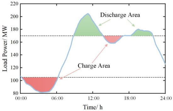
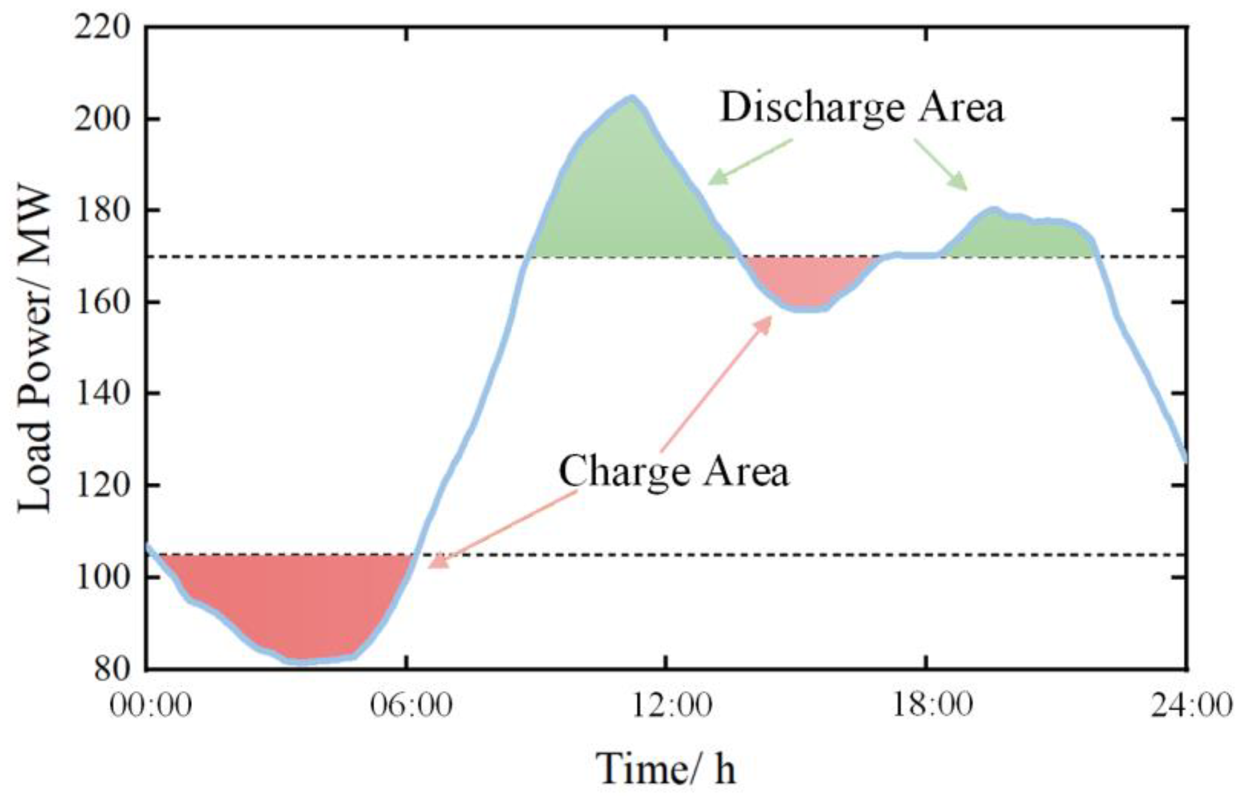
The operational principle of a BESS in peak shaving and valley filling scenarios is to discharge electricity during periods of peak load and charge during periods of valley load, thereby alleviating the peak shaving and valley filling burden on conventional thermal power units and achieving temporal and spatial energy shifting. For the distribution network, the flatter the load profile after BESS participation, the more effective the peak shaving and valley filling performance, as shown in Figure 1.

Figure 1. Schematic diagram of BESS participation in peak shaving and valley filling scenarios.

Variance characterizes the degree to which a random variable deviates from its central value and reflects the dispersion of its distribution [25]. Based on this definition, the load variance can be used to quantify the flatness of the load curve; a smaller variance indicates a better peak shaving and valley filling effect. Therefore, this paper adopts the load variance after BESS participation as the technical indicator, as expressed in Equation (9):

$$S^2={\displaystyle \frac{1}{N}}{\displaystyle \sum _{i=0}^N[(P_{\mathrm{load}\_i}-(P_{\mathrm{bess}\_i}^{\mathrm{dis}}+P_{\mathrm{bess}\_i}^{\mathrm{ch}}))}-{\displaystyle \frac{1}{N}}{\displaystyle \sum _{i=0}^N(P_{\mathrm{load}\_i}-(P_{\mathrm{bess}\_i}^{\mathrm{dis}}+P_{\mathrm{bess}\_i}^{\mathrm{ch}}))}{]}^2$$

(9)

where P_{load_i} represents the load value at time i when the BESS is not participating in peak shaving and valley filling.

Meanwhile, to quantify the impact of BESS integration on peak shaving, the absolute peak-to-valley difference and the peak reduction rate are selected as technical indicators:

$$\Delta P_{\mathrm{PV}}=P_{\max }-P_{\min }$$

(10)

$${\eta }_{\mathrm{PV}}={\displaystyle \frac{P_{\max ,\mathrm{ori}}-P_{\max ,\mathrm{bess}}}{P_{\max ,\mathrm{ori}}}}$$

(11)

where ΔP_PV denotes the peak-to-valley difference; P_max represents the maximum load power; P_min represents the minimum load power; η_PV denotes the peak reduction rate; P_max,ori denotes the maximum value of the original load power; and P_max,bess denotes the maximum load power after peak shaving and valley filling with the participation of the BESS.

3. Optimization Model of BESS for Peak Shaving and Valley Filling Scenarios

3.1. Objective Functions

Based on the analysis in Section 2, the economic and technical indicators of the BESS participating in peak shaving and valley filling scenarios have been determined. The economic objective aims to maximize the annual revenue, as given in Equation (8), while the technical objective seeks to minimize the load variance after BESS participation in peak shaving and valley filling, as given in Equation (9). Accordingly, the objective function can be formulated as follows:

$$\max \hspace{1em}{I}_{\mathrm{total}\_\mathrm{tf}}=I_{\mathrm{tf}}+I_{\mathrm{e}}+I_{\mathrm{sy}}-C_{\mathrm{t}}-C_{\mathrm{y}}-C_{\mathrm{b}}$$

(12)

$$\min \hspace{1em}{S}^2$$

(13)

3.2. Constraints

3.2.1. Charge/Discharge Power Constraints

The charge and discharge power of the BESS must not exceed its rated power P_m, and therefore the following constraint must be satisfied:

$$\left\{\begin{array}{c}0\le P_{\mathrm{bess}\_i}^{\mathrm{dis}}\le P_{\mathrm{m}}\\ -P_{\mathrm{m}}\le P_{\mathrm{bess}\_i}^{\mathrm{ch}}\le 0\end{array}\right.$$

(14)

As mentioned earlier, the discharge power is defined as positive, while the charge power is defined as negative.

3.2.2. SOC Constraints

The capacity of the BESS is limited, and excessive charge or discharge accelerates battery degradation and may lead to failure. Therefore, the SOC must be maintained within a reasonable range. At time t, the SOC is calculated as follows:

$$SOC(t)={\displaystyle \frac{E_0-{\displaystyle {\int }_0^i(P_{\mathrm{bess}\_i}^{\mathrm{dis}}+P_{\mathrm{bess}\_i}^{\mathrm{ch}})dt}}{E_{\mathrm{m}}}}$$

(15)

where E₀ represents the initial capacity of the BESS. To ensure reliable operation of the BESS, the SOC must satisfy the following constraint:

$$SO{C}_{\min }\le SOC(t)\le SO{C}_{\max }$$

(16)

where SOC_min and SOC_max represent the minimum and maximum allowable values of SOC, respectively. The BESS considered in this paper adopts lithium iron phosphate batteries; therefore, SOC_min is set to 0.1 and SOC_max is set to 0.9 [26].

3.2.3. Charge/Discharge State Constraint

At any given time, BESS can operate in only one of three states: charge, discharge, or idle. Accordingly, the states are defined as follows: during charge state, S_ch = 1 and S_dis = 0; during discharge state, S_dis = 1 and S_ch = 0; during idle, S_ch = S_dis = 0. Based on this, the charge/discharge state constraint can be expressed as follows:

$$S_{\mathrm{dis}}+S_{\mathrm{ch}}\le 1$$

(17)

where S_dis represents the state of discharge and S_ch represents the state of charge.

3.2.4. Energy Balance Constraint

For peak shaving and valley filling scenarios, it is required that, within one day, the energy discharged by the BESS for peak shaving equals the energy absorbed during valley filling. That is, the BESS must achieve energy balance within a day, and its SOC needs to be restored to the initial level. Therefore, the following constraint must be satisfied (Equation (18)):

$${\displaystyle {\int }_0^N{P}_{\mathrm{bess}\_i}^{\mathrm{dis}}dt={\displaystyle {\int }_0^N-P_{\mathrm{bess}\_i}^{\mathrm{ch}}dt}}$$

(18)

The energy balance constraint is introduced to ensure the long-term sustainability of peak shaving and valley filling operation. Since day-ahead load profiles typically exhibit consistent intra-day variation patterns over extended periods, the BESS is required to operate in repetitive daily charge/discharge cycles within similar time windows. Forcing the SOC to return to its initial level at the end of each 24 h period guarantees that the BESS maintains sufficient operational flexibility for subsequent days, thereby preventing energy drift and ensuring stable long-term peak shaving and valley filling performance at the planning stage.

3.3. Methods

Building upon the analyses presented in Section 3.1 and Section 3.2, this study develops an optimization model for BESS capacity configuration under peak shaving and valley filling scenarios. This model is inherently a multi-objective optimization problem. Traditional solution approaches typically convert a multi-objective optimization problem into a single-objective one and then map the obtained solution back to the multi-objective context. Common methods include the weighted-sum method [27], goal programming [28], etc. However, these approaches usually yield only a single optimal solution and, when combined with intelligent optimization algorithms, are prone to local optima, thereby affecting the overall optimization performance.

To address these limitations, this paper proposes a solution strategy that integrates the MOPSO algorithm with the TOPSIS method. First, the MOPSO algorithm is employed to directly solve the multi-objective optimization model and obtain a Pareto-optimal solution set that satisfies all constraints. Each Pareto solution is a non-dominated solution to the optimization problem, and together they form the Pareto frontier. On this basis, the TOPSIS method is introduced to evaluate the relative closeness of each non-dominated solution to the ideal solution. The solution with the shortest distance to the ideal point is selected as the final optimal configuration, thereby determining the BESS capacity configuration.

3.3.1. Multi-Objective Particle Swarm Optimization

The MOPSO algorithm extends the basic particle swarm optimization framework by incorporating Pareto dominance relationships and multi-objective fitness evaluation. This enables the algorithm to obtain a Pareto-optimal solution set, providing multiple feasible solutions to the optimization problem while simultaneously satisfying all objectives.

The three basic parameters of PSO are particle position, velocity and fitness value. The basic principle of PSO is interpreted in [29]. The specific formulation is given as follows:

$$\begin{array}{l}{v}_i^{d+1}=\omega v_i^d+c_1{r}_1(P_{best\_i}^d-x_i^d)+c_2{r}_2(G_{best}^d-x_i^d)\\ x_i^{d+1}=x_i^d+v_i^{d+1}\end{array}$$

(19)

where d is the iteration number; $x_i^d$ and $v_i^d$ are the position and velocity of particle i at the d-th iteration; ω is the inertia weight; c₁ and c₂ are the individual learning factors and the global learning factors; r₁ and r₂ are random numbers between 0 and 1; and $P_{best\_i}^d$ and $G_{best}^d$ are the particle’s best position and the global best position, respectively.

Usually, the value of ω linearly decreases according to the number of iterations:

$${\omega }_d={\omega }_{\max }-{\displaystyle \frac{{\omega }_{\max }-{\omega }_{\min }}{d_{\max }}}\times d$$

(20)

where ω_max and ω_min are the upper and lower limit of ω and d_max is the maximum number of iterations.

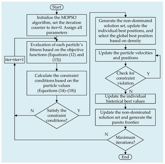
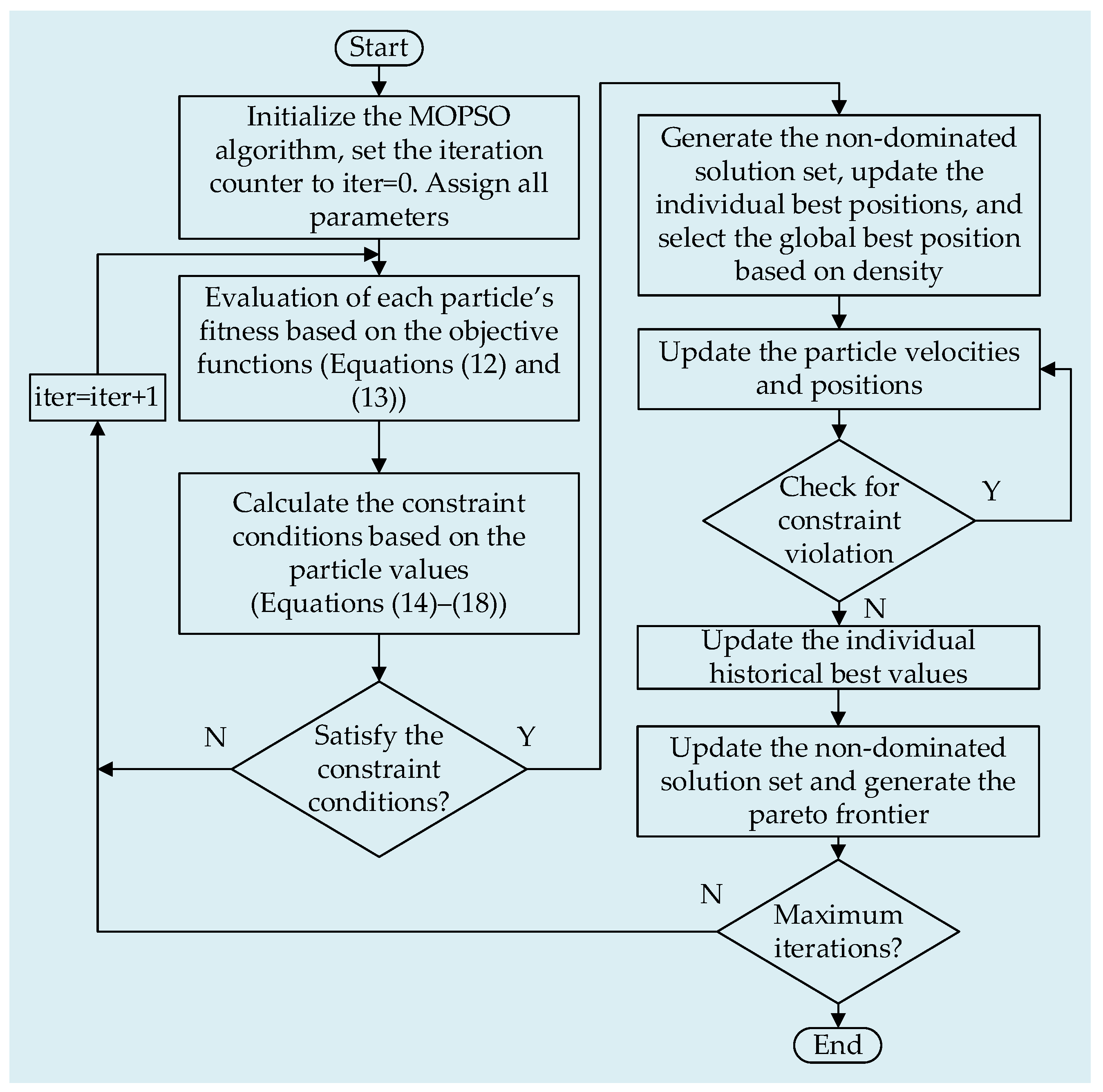
The MOPSO algorithm used in this paper follows the procedure outlined below:

• First, initialize the particle parameters, set the iteration count to 0, and assign the values for all relevant parameters.
• According to Equations (12) and (13), calculate the fitness of each particle.
• Based on the current particle values, it is checked whether the constraints given in Equations (14)–(18) are satisfied.
• If the constraints are satisfied, proceed to step 5; otherwise, increment the iteration count by one and return to step 2.
• The Pareto-optimal solutions are identified based on the fitness of all particles to generate the non-dominated solution set, and the individual best positions of the particles are updated; the global best position is then selected according to density.
• Update the positions and velocities of the particles.
• Check whether the particles’ positions and velocities exceed their limits. If they are within the limits, proceed to step 8; otherwise, return to step 6.
• Update the historical best values of each particle.
• Update the non-dominated solution set and generate the Pareto frontier.
• Determine whether the current iteration count has reached the maximum number of iterations. If not, increment the iteration count by one and return to step 2.
• Output the Pareto-optimal solution set and terminate the algorithm.

The detailed solution flowchart is shown in Figure 2:

Figure 2. MOPSO solution process.

3.3.2. Technique for Order Preference by Similarity to Ideal Solution

Since MOPSO yields a Pareto frontier composed of multiple non-dominated solutions, each solution on the Pareto frontier can be regarded as an optimal scheme in the multi-objective sense. Therefore, further selection among these configurations is necessary. Based on this, the TOPSIS method is employed to rank the Pareto solutions, identifying the configuration closest to the ideal solution as the optimal BESS capacity configuration.

First, the decision matrix X needs to be constructed. Assume that there are m alternatives and n evaluation criteria:

$$X=\left[\begin{array}{cccc}{x}_{11}& x_{12}& \dots & x_{1n}\\ x_{21}& x_{22}& \dots & x_{2n}\\ ⋮& ⋮& \ddots & ⋮\\ x_{m1}& x_{m2}& \dots & x_{mn}\end{array}\right]$$

(21)

Then, the decision matrix X is normalized according to Equation (22):

$$z_{ij}={\displaystyle \frac{x_{ij}}{\sqrt{{\displaystyle \sum _{i=1}^m{x}_{ij}^2}}}}$$

(22)

where z_ij is the element of the normalized matrix Z and x_ij is the element of the decision matrix X (i = 1, 2…m; j = 1, 2…n). The normalized matrix Z is shown as follows:

$$Z=\left[\begin{array}{cccc}{z}_{11}& z_{12}& \dots & z_{1n}\\ z_{21}& z_{22}& \dots & z_{2n}\\ ⋮& ⋮& \ddots & ⋮\\ z_{m1}& z_{m2}& \dots & z_{mn}\end{array}\right]$$

(23)

The normalized matrix Z can be used to determine two idealized objectives: the positive ideal solution Z⁺ and the negative ideal solution Z⁻:

$$\begin{array}{cc}\hfill Z^{+}& =[z_1^{+},z_2^{+},\dots ,z_n^{+}]\hfill \\ & =[\max \left\{z_{11},z_{21},\dots z_{m1}\right\},\max \left\{z_{12},z_{22},\dots z_{m2}\right\},\dots ,\max \left\{z_{1n},z_{2n},\dots z_{mn}\right\}]\hfill \end{array}$$

(24)

$$\begin{array}{cc}\hfill Z^{-}& =[z_1^{-},z_2^{-},\dots ,z_n^{-}]\hfill \\ & =[\min \left\{z_{11},z_{21},\dots z_{m1}\right\},\min \left\{z_{12},z_{22},\dots z_{m2}\right\},\dots ,\min \left\{z_{1n},z_{2n},\dots z_{mn}\right\}]\hfill \end{array}$$

(25)

The positive ideal solution represents the scenario in which all objective attributes achieve their optimal values, while the negative ideal solution corresponds to the scenario in which all objective attributes take their worst values.

Next, the distance of each alternative to the positive and negative ideal solutions is calculated as follows:

$$d_i^{+}=\sqrt{{\displaystyle \sum _{j=1}^n{(z_j^{+}-z_{ij})}^2}}$$

(26)

$$d_i^{-}=\sqrt{{\displaystyle \sum _{j=1}^n{(z_j^{-}-z_{ij})}^2}}$$

(27)

where $d_i^{+}$ represents the distance of the i-th alternative to the positive ideal solution and $d_i^{-}$ represents the distance to the negative ideal solution. In this study, equal weights are assigned to the economic and technical indicators; therefore, no weighting coefficients are introduced in the calculations of Equations (26) and (27).

Finally, the closeness of each alternative to the ideal solution is calculated based on these distances:

$$S_i={\displaystyle \frac{d_i^{-}}{d_i^{+}+d_i^{-}}}$$

(28)

where S_i represents the closeness of the i-th alternative to the worst solution. A larger S_i value indicates that the alternative is farther from the worst solution and closer to the optimal solution. By comparing the S_i values of all alternatives, the optimal solution can be identified.

4. Case Study on the Typical Daily Load Curve

4.1. Paramaters

This paper considers a lithium iron phosphate (LFP)-based BESS installed on the distribution network side for peak shaving and valley filling applications. The detailed parameters of the BESS are given in Table 1 [30], and the subsidy standard is based on the Implementation Rules for Ancillary Service Management in the Southern Regional Power Market of China.

Table 1. Parameter values used for capacity optimization.

Parameter	Value	Parameter	Value
Mp	150 (10,000 CNY/MW)	n	10.5 (annual)
Me	350 (10,000 CNY/MWh)	Cinv	300 (10,000 CNY/MW)
Np	2 (10,000 CNY/MW)	it	1.5%
Ne	0.05 (10,000 CNY/MWh)	id	4.5%
λpcs	0.7 (10,000 CNY/MW)	αecs	2.5 (10,000 CNY/MWh)

Based on the data in Table 1, the average service life n of the LFP-based BESS is 10.5 years. The SOC limits of the BESS are set to 0.1–0.9.

The parameter indicators for environmental revenue are taken from the data in reference, as shown in Table 2:

Table 2. Types of pollutants and environmental treatment cost.

Pollutant	Parameter	Value	Parameter	Value
Dust	G1	0.5 (kg/MWh)	R1	2.918 (CNY/kg)
SO2	G2	0.5 (kg/MWh)	R2	6.235 (CNY/kg)
NOx	G3	0.75 (kg/MWh)	R3	8.03 (CNY/kg)
CO2	G4	0.3 (kg/MWh)	R4	0.024 (CNY/kg)
CO	G5	0.05 (kg/MWh)	R5	1.009 (CNY/kg)

4.2. Typical Daily Load Analysis

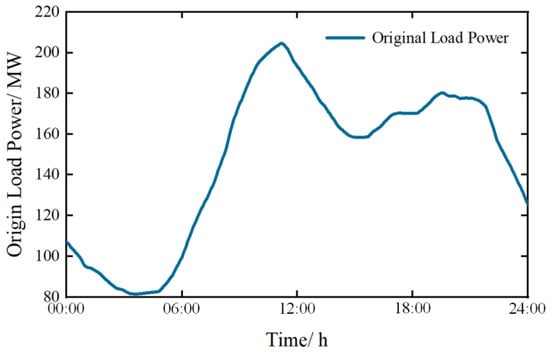
The simulation analysis in this study uses typical daily load data from a region in southern China. The profile represents a commonly observed intra-day load pattern, as shown in Figure 3. The time period spans from 0 to 24 h, with a sampling interval of Δt = 1 min, resulting in a total of N = 1440 sampling points.

Figure 3. Original load power.

In this paper, the maximum number of iterations for the MOPSO algorithm is set to 100 to solve the optimization model of the BESS for peak shaving and valley filling scenarios that simultaneously considers economic and technical indicators. The remaining parameters of the MOPSO algorithm are listed in Table 3 [30]:

Table 3. MOPSO parameters.

Parameter	Value
Population size	100
Pareto set size	100
dmax	100
c1, c2	1.05
ωmax	0.9
ωmin	0.4

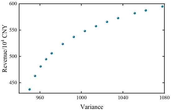
After running the algorithm, the resulting Pareto frontier is shown in Figure 4:

Figure 4. Pareto frontier under peak shaving and valley filling scenarios.

As shown in Figure 4, as the variance of peak shaving and valley filling gradually decreases, the corresponding revenue also declines. This occurs because achieving better technical indicator performance requires increasing the BESS’s power and energy capacity, which raises the investment cost and consequently reduces the net revenue.

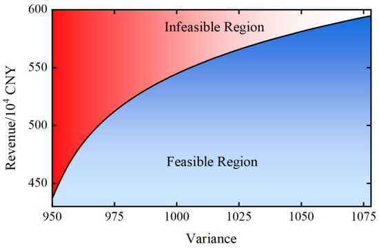
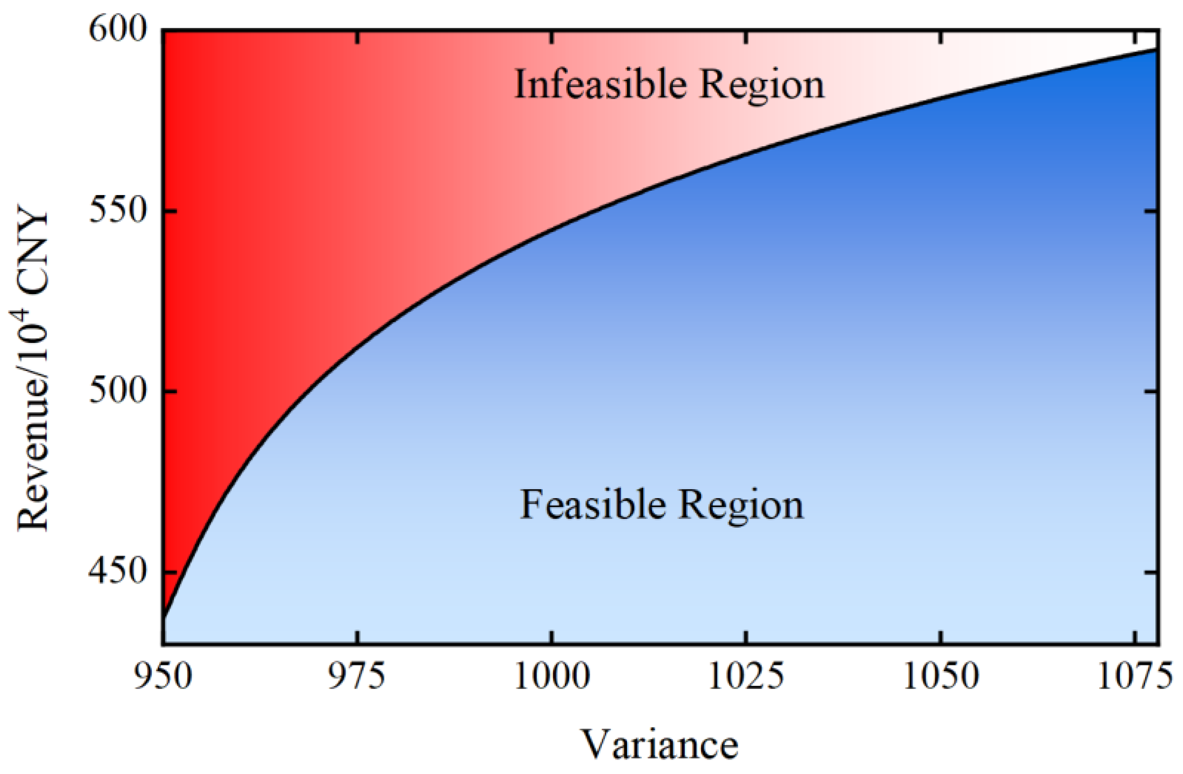
Furthermore, based on the Pareto frontier in Figure 4, the feasible and infeasible regions for achieving the economic and technical indicators of the BESS under this scenario can be identified in Figure 5.

Figure 5. Feasible/infeasible regions of the two indicators.

Based on the analysis in Section 3.3, the obtained Pareto frontier solution set consists of multiple non-dominated solutions. Therefore, following the procedure described in Section 3.3.2, the TOPSIS method is applied to select the optimal solution from 14 candidate schemes.

Among the two optimization objectives, a larger revenue is preferred, while a smaller technical indicator (variance) is better. To unify the monotonicity of these two indicators, the technical indicator is first converted into a positive form:

$$\min \hspace{1em}{S}^2=\max \hspace{1em}{\displaystyle \frac{1}{S^2}}$$

(29)

Then, these 14 solutions are normalized to construct the normalized matrix Z (the normalized matrix Z is shown in Appendix A.1, Table A1).

Thus, the positive ideal solution Z⁺ and the negative ideal solution Z⁻ are as follows:

$$Z^{+}=[0.213012552,0.217329922]$$

(30)

$$Z^{-}=[0.187719781,0.159786569]$$

(31)

According to Equations (26) and (27), the distances from the positive ideal solution and the negative ideal solution for each scheme can be calculated. The results are provided in Appendix A.2, Table A2.

Accordingly, the closeness coefficient of each solution to the worst solution can be obtained using Equation (28), based on which the optimal solution within the non-dominated solution is determined. The closeness coefficients of all candidate solutions are provided in Appendix A.3, Table A3.

According to Table A3, Solution 6 is identified as the optimal choice. In this configuration, the BESS is sized with a power rating of 27.7 MW and an energy capacity of 78.3 MWh. The corresponding peak shaving and valley filling variance is 1035.33, and the annual average revenue reaches 5.7258 million CNY.

To compare the advantages of the proposed method, two additional characteristic points were selected and compared with the optimal solution obtained in this paper. The two selected points correspond to the solution with the minimum variance and the solution with the maximum revenue within the non-dominated solution sets. Their corresponding indicators are presented in Table 4, while the BESS configuration details are shown in Table 5.

Table 4. Indicators of characteristic points.

Characteristic Point	Variance	Absolute Peak–Valley Difference (MW)	Peak Reduction Rate	Revenue (104 CNY)
Minimum variance point	950	76.43	14.28%	437.29
Maximum revenue point	1078	80.12	8.73%	594.77
TOPSIS optimal point	1035.33	77.13	13.52%	572.58

Table 5. BESS configuration of characteristic points.

Characteristic Point	Rated Power (MW)	Rated Capacity (MWh)
Minimum variance point	36.2	82.1
Maximum revenue point	25.9	71.6
TOPSIS optimal point	27.7	78.3

From Table 4 and Table 5, it can be observed that the proposed method, by reasonably configuring the power and capacity of the BESS, simultaneously reduces the load variance while maximizing economic benefits to the greatest extent, thereby demonstrating the feasibility of the approach.

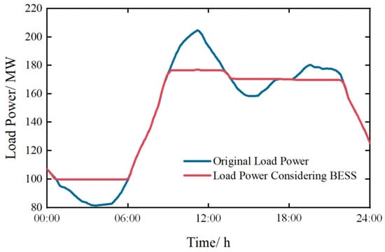
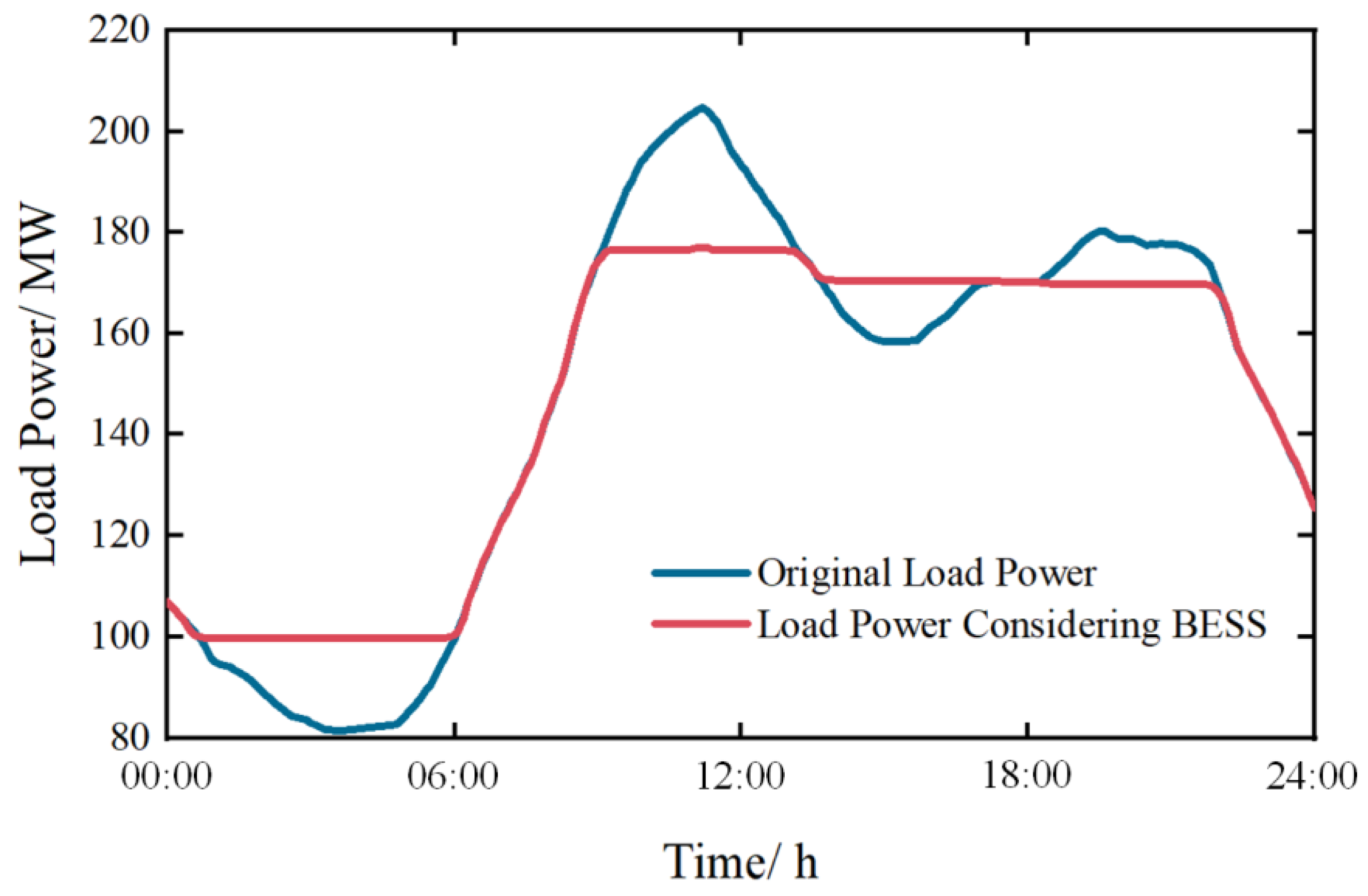
The original load power and the load power after BESS participation in peak shaving and valley filling are shown in Figure 6.

Figure 6. Comparison of original load power and load power after BESS participation.

As shown in Figure 6, the BESS charges during valley periods and discharges during peak periods, resulting in a smoother load power curve and reducing the peak shaving and valley filling burden on conventional thermal power units.

Meanwhile, the original load variance is 1525.89. After BESS participation in peak shaving and valley filling, the variance is reduced to 1035.33, representing a 32.15% decrease. The peak of the original load curve is 204.83 MW. After peak shaving with the BESS, the peak is reduced to 177.13 MW, achieving a peak reduction rate of 13.5%.

The annual average revenue of the BESS participating in the peak shaving and valley filling scenario is 5.7258 million CNY. The corresponding economic indicators are presented in Table 6.

Table 6. Economic indicators.

	Cost (104 CNY)	Revenue (104 CNY)
Investment cost	3005.71	0
Operation and maintenance costs	59.32	0
Decommissioning cost	−16.80	0
Peak shaving/valley filling revenue	0	3176.72
Environmental revenue	0	32.50
Deferred grid investment revenue	0	411.59

Table 6 summarizes the annual economic indicators of the optimized BESS configuration. On the cost side, the investment cost accounts for the largest proportion of the total cost. This is mainly because the capital expenditure of a BESS is directly determined by both the rated power and rated capacity, including battery modules and power conversion equipment. In contrast, operation and maintenance costs are relatively small. Since the decommissioning cost includes the residual value recovered from the BESS batteries, this item is negative.

On the revenue side, peak shaving/valley filling revenue constitutes the largest share of total income. This indicates that the configured BESS power and capacity enable effective participation in peak shaving and valley filling services, allowing the system to fully utilize the subsidy mechanism during charging and discharging periods. The dominance of this revenue component verifies the feasibility and rationality of the proposed BESS configuration for peak shaving and valley filling applications.

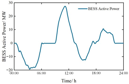
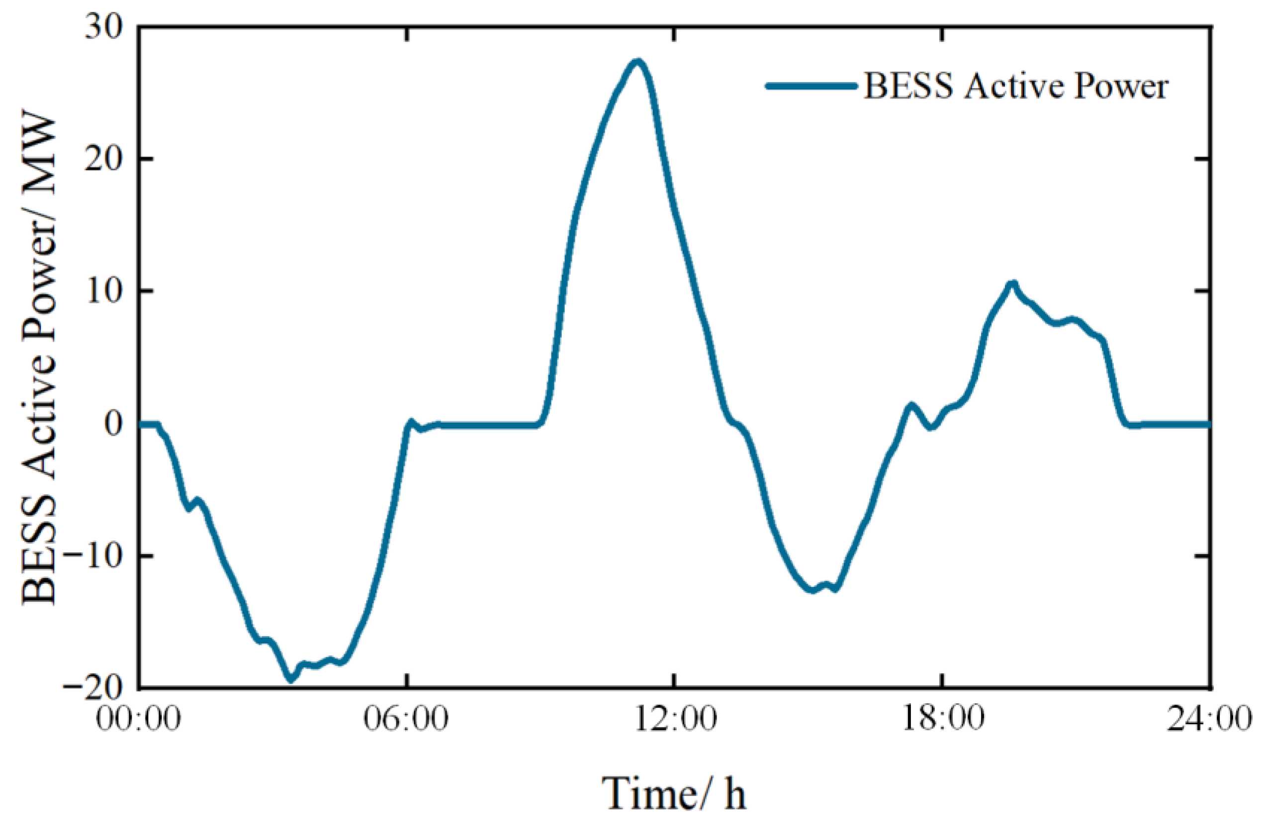
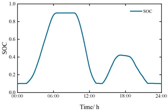
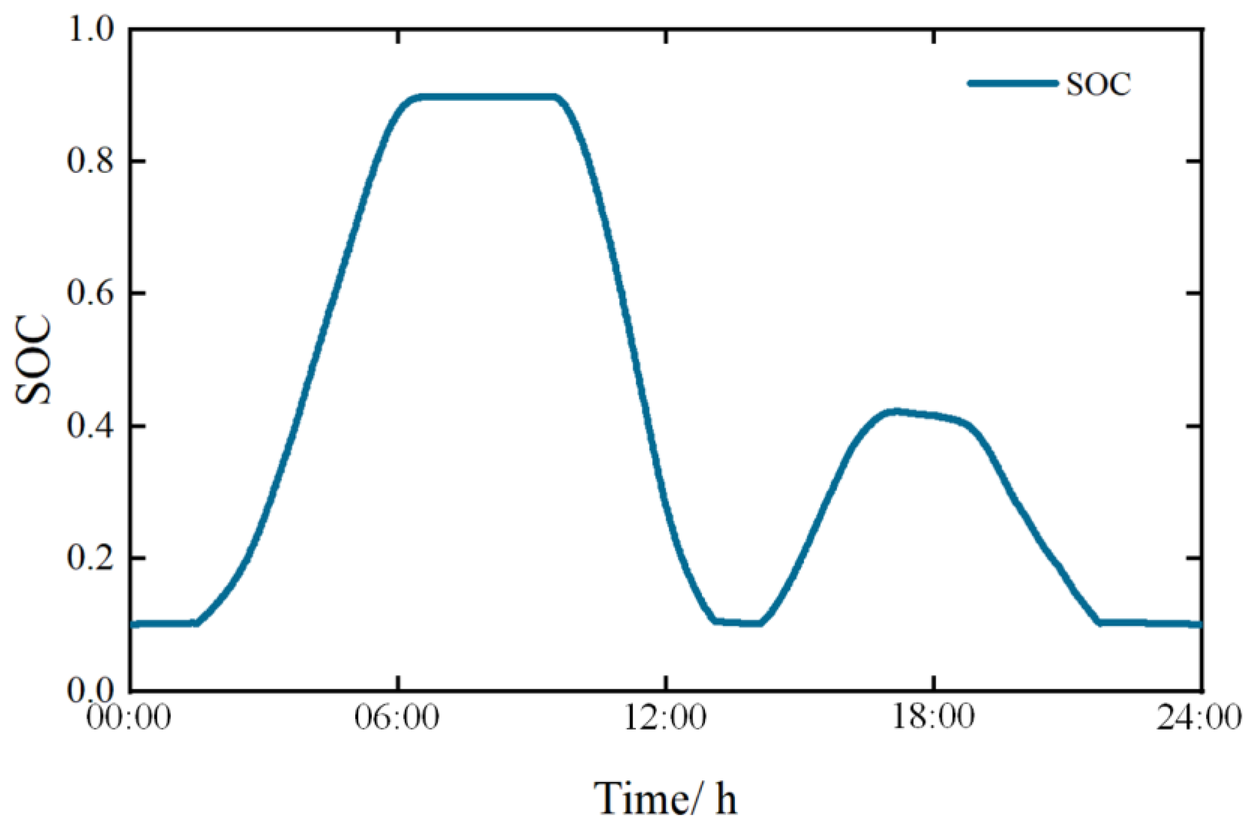
Figure 7 and Figure 8 respectively illustrate the active power output of the BESS during the peak shaving and valley filling periods and the corresponding SOC.

Figure 7. BESS output power in the peak shaving and valley filling scenarios.

Figure 8. BESS state of charge.

According to Figure 7, the BESS absorbs energy during the early-morning valley load periods and releases it during the midday peak load periods. It then charges again in the afternoon and discharges during the evening peak load periods, thereby accomplishing peak shaving and valley filling. Meanwhile, the maximum charge/discharge power reaches 27.43 MW, which is lower than the rated power configured for the system.

Figure 8 illustrates the daily SOC trajectory of the BESS. The SOC remains within the specified limits throughout the entire operating period and exhibits an overall pattern of two charging cycles and two discharging cycles. Moreover, the total charging and discharging energies are balanced, and the final SOC returns to approximately its initial value of 0.1. This verifies the reliability of the simulation results.

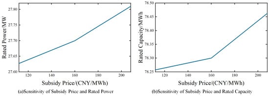
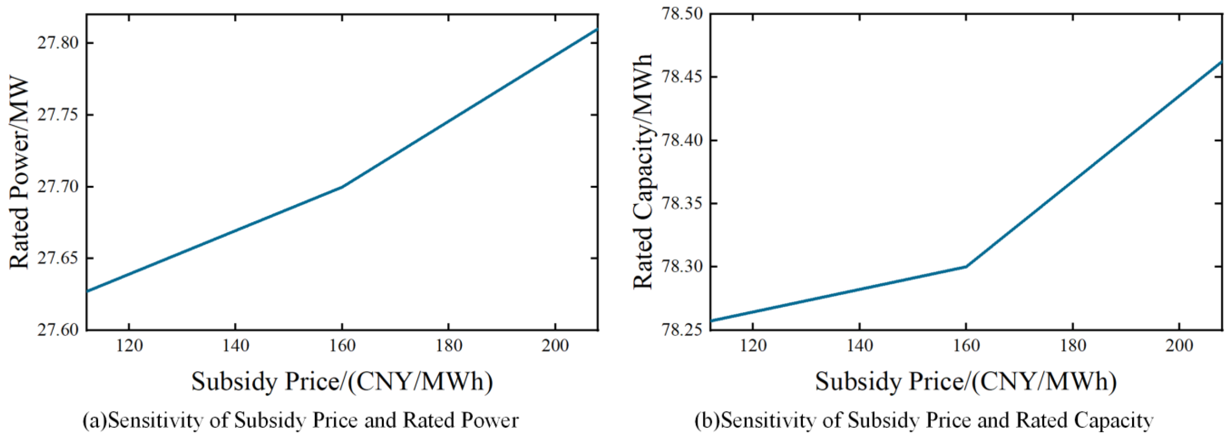
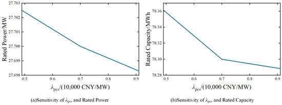
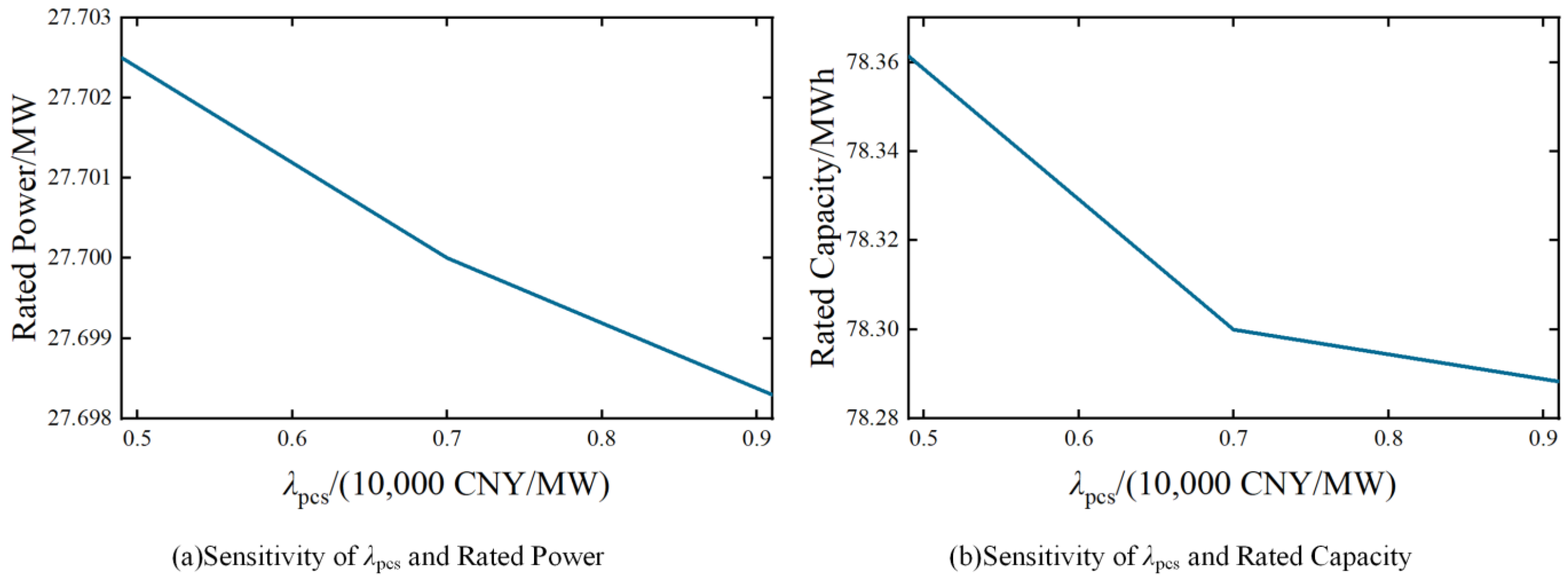
To further evaluate the robustness of the proposed configuration framework, sensitivity analyses are conducted with respect to two key economic parameters: the subsidy price and the λ_pcs. These parameters directly affect the economic objective and may potentially influence the optimal rated power (P_m) and rated energy capacity (E_m) of BESS.

In this study, each parameter is varied within ±30% of its baseline value while keeping all other variables unchanged. Specifically, the subsidy price is adjusted around the base value of 160 CNY/MWh, and λ_pcs is adjusted around the baseline value of 0.7 (10,000 CNY/MW). For each parameter variation, the optimization process is re-executed to obtain the corresponding optimal configuration results.

Figure 9 and Figure 10 illustrate the sensitivity of rated power and rated capacity to variations in subsidy price and λ_pcs, respectively. It can be observed that, within the considered variation range, both P_m and E_m exhibit only minor fluctuations. Compared with the subsidy price, the influence of λ_pcs on the optimal configuration is even weaker.

Figure 9. Sensitivity of subsidy and rated power/capacity.

Figure 10. Sensitivity of λ_pcs and rated power/capacity.

To quantitatively assess sensitivity, the variance of the obtained configuration results under different parameter settings is calculated, as shown in Table 7. The computed variances of P_m and E_m are very small in both cases, indicating that the proposed multi-objective configuration framework maintains stable optimization outcomes under moderate economic parameter perturbations.

Table 7. Sensitivity variance indicators.

Sensitivity Indicators	Variance
Subsidy price—Rated Power	8.50 × 10−3
Subsidy price—Rated Capacity	1.17 × 10−2
λpcs—Rated Power	4.46 × 10−6
λpcs—Rated Capacity	1.50 × 10−3

These results demonstrate that the optimal BESS configuration is not overly sensitive to individual economic parameters, reflecting the robustness and structural stability of the proposed MOPSO–TOPSIS framework.

To demonstrate the advantages of the proposed method, a comparative analysis is conducted between this method and the weighted-sum method presented in [27]. The results are shown in Table 8.

Table 8. Comparison of the results obtained by the two methods.

	Rated Power	Rated Capacity	Revenue	Variance
Weighted-sum method	30.27 MW	50.78 MWh	533.24 (104 CNY)	1052.67
Proposed method	27.7 MW	78.3 MWh	572.58 (104 CNY)	1035.33

As shown in Table 8, the proposed method demonstrates superior performance in both economic and technical indicators compared with the weighted-sum method. This superiority arises from the ability of the proposed framework to explicitly capture the interactions and trade-offs between the two optimization objectives through the construction of the Pareto frontier, thereby generating solutions that are more suitable for peak shaving and valley filling applications.

In contrast, the weighted-sum method converts the multi-objective optimization problem into a single-objective formulation. The resulting solution strongly depends on the predefined weight coefficients and may only be optimal under specific weight settings. Such a formulation increases the risk of convergence to local optima, and therefore the obtained configuration may not represent the true global optimum.

4.3. Comparisons of Performance of the MOPSO and NSGA-II

To verify the superiority of the MOPSO algorithm adopted in this study, a comparison is conducted with the NSGA-II algorithm in [31]. Two metrics are used to quantitatively evaluate the results of the two algorithms: Spacing (S metric) and Maximum Spread (M metric) [32].

Before the comparison, the economic indicator is processed. A larger value is preferred. Therefore, following the approach in Equation (29), the reciprocal of the economic indicator is used. A larger revenue then corresponds to a smaller value. This is consistent with the optimization objective of the iterative algorithm. The economic indicator is denoted as f₁. The technical indicator is denoted as f₂.

The density distance defined in Equation (32) is used to characterize the density between a particle and its surrounding particles, and can be used to describe the uniformity of the solution set:

$$D_i={\displaystyle \sum _{k=1}^2\frac{\left|f_{i,k}^l-f_{i,k}^r\right|}{f_k^{\max }}}$$

(32)

where D_i is the density distance of the i-th particle; k denotes the number of objective functions (k_max = 2 due to there are two objective functions); $f_k^{\max }$ is the maximum value of the k-th objective function; and $f_{i,k}^l$ and $f_{i,k}^r$ are the two particle closest to it.

The S metric is used to evaluate the uniformity of the population distribution and is defined in Equation (33). A larger value indicates a more non-uniform distribution.

$$S=\sqrt{{\displaystyle \frac{1}{n_p}}{\displaystyle \sum _{i=1}^{n_p}{(D_i-\overline{D})}^2}}$$

(33)

where n_p is the size of the Pareto solution set and $\overline{D}$ is the average value of D_i.

M metric uses the maximum extent in each dimension to estimate the range to which the front spreads out. However, in the proposed optimization problem, the two objective functions are characterized by different physical meanings and units, leading to significant differences in numerical scales. Direct computation of the M metric based on the original objective values may therefore result in biased or physically meaningless evaluations.

To address this issue, all objective functions are first normalized into a dimensionless form before calculating the spread-related metric. The normalized objective value ${\widehat{f}}_{i,k}$ of the i-th solution with respect to the k-th objective is defined as follows:

$${\widehat{f}}_{i,k}={\displaystyle \frac{f_{i,k}-f_k^{\min }}{f_k^{\max }-f_k^{\min }}}$$

(34)

where $f_k^{\min }$ is the minimum value of the k-th objective function. Based on the normalized objective values, the M metric is calculated as follows:

$$M=\sqrt{{\displaystyle \sum _{k=1}^2{({\widehat{f}}_k^{\max }-{\widehat{f}}_k^{\min })}^2}}$$

(35)

Where ${\widehat{f}}_k^{\max }$ and ${\widehat{f}}_k^{\min }$ denote the maximum and minimum normalized values of the k-th objective function in the Pareto set.

A larger value of M indicates that the Pareto solutions cover a wider region of the objective space, demonstrating stronger global search capability and better exploration performance of the algorithm.

Both algorithms are executed 10 times, with the same population size and the same maximum number of iterations to ensure a fair comparison. The average values of S, M, and the two objective functions are calculated. The results are shown in Table 9. As shown in the table, compared with NSGA-II, MOPSO yields a smaller S metric and a larger M metric. This indicates that the obtained non-dominated solutions are widely and uniformly distributed in the solution space. Good diversity is achieved.

Table 9. Results of the two algorithms.

Algorithms	S	M	f1	f2
MOPSO	0.041	1.02	1.68 × 10−7	916.69
NSGA-II	0.118	0.63	1.74 × 10−7	940.34

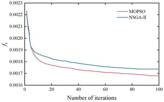
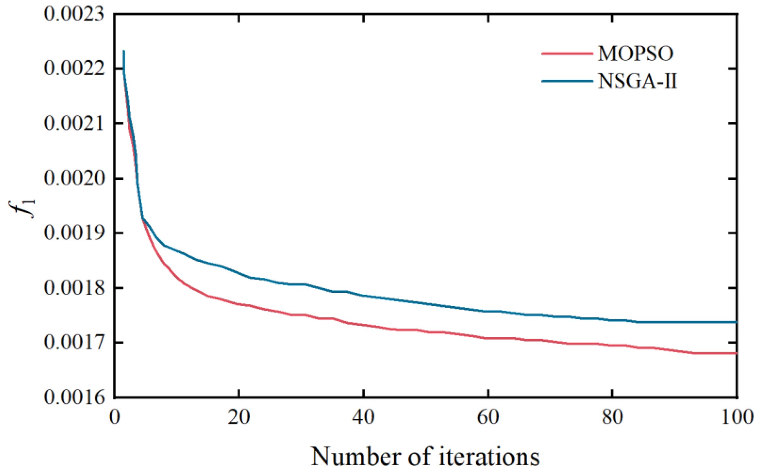
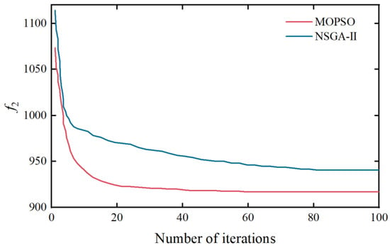
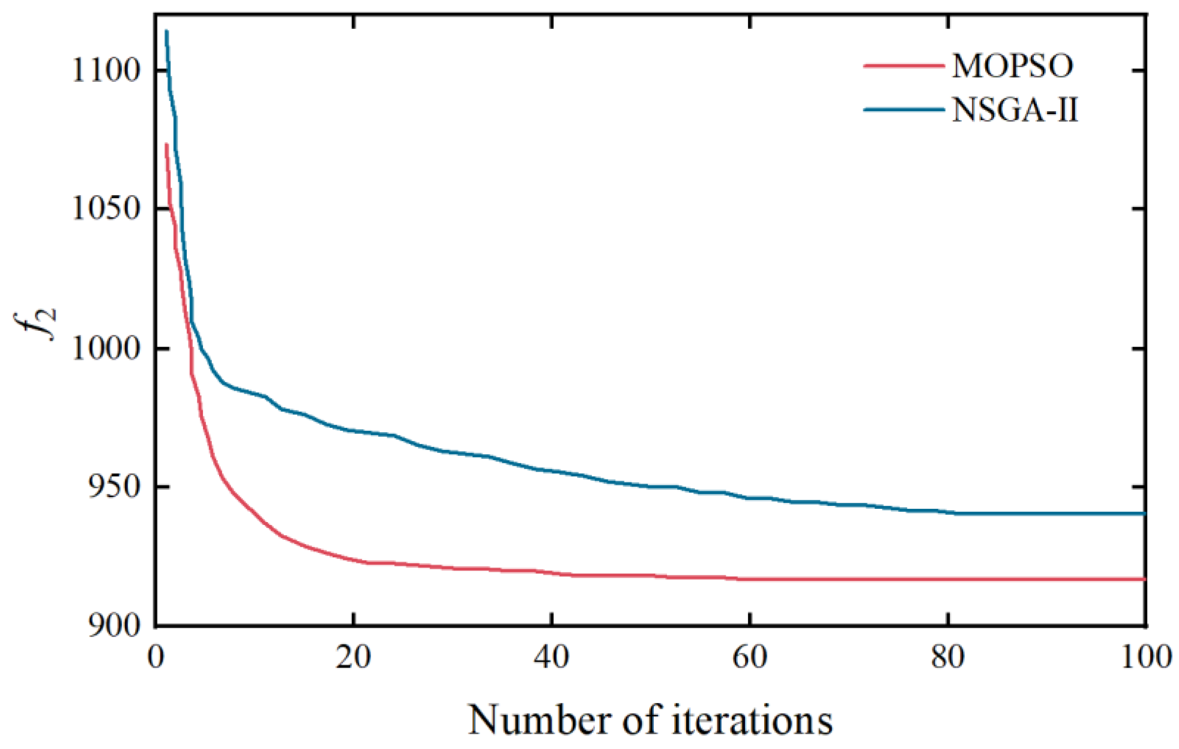
To compare the convergence speed of MOPSO and NSGA-II, the convergence processes of objective functions f₁ and f₂ are plotted. They are shown in Figure 11 and Figure 12, respectively:

Figure 11. Convergence process of f₁.

Figure 12. Convergence process of f₂.

As shown in Figure 11 and Figure 12, compared with NSGA-II, the MOPSO algorithm achieves smaller objective function values. Faster convergence is also observed. Based on the above results, the rationality and effectiveness of the MOPSO algorithm adopted in this study are verified.

Table 10 shows the standard deviation of the two indicators.

Table 10. Standard deviation of the two indicators.

Algorithm	Standard Deviation of f1	Standard Deviation of f2
MOPSO	0.00124	457.59
NSGA-II	0.00139	464.03

5. Case Study on the WSCC 9-Bus System with PV Integration

To further verify the applicability and scalability of the proposed multi-objective optimization framework in renewable-energy integrated power systems, the case study is extended to the classical WSCC 9-bus system, with PV generation. The reduction in node voltage fluctuations is investigated under PV penetration. This is achieved through appropriate power and capacity configuration of the BESS.

5.1. Newly Added Objective Function

In addition to satisfying the economic and technical indicators, system node voltage must also be ensured. Node voltage is a critical indicator of system stability and power quality. The voltage at each node should be maintained within a prescribed range, and excessive voltage fluctuations must be avoided. The peak–valley characteristics of the load, together with the variability of PV output, can induce node voltage fluctuations and adversely affect power system stability. Therefore, node voltage fluctuation is selected as the newly added objective function:

$$\min \hspace{1em}\Delta U_{\mathrm{n}}={\displaystyle \sum _{\mathrm{n}=1}^9{\displaystyle \sum _{\mathrm{t}=1}^{24}\left|U_{\mathrm{n},\mathrm{t}}-{\overline{U}}_{\mathrm{n}}\right|}}$$

(36)

where n represents the number of nodes, t represents the number of hours, U_n,t denotes the voltage of node n at time t, and ${\overline{U}}_{\mathrm{n}}$ denotes the average voltage of node n.

5.2. Newly Added Constraints

• Power balance constraint:

$${\displaystyle \sum _{i=1}^{N_{\mathrm{G}}}{P}_{\mathrm{G},i}(\mathrm{t})}+P_{\mathrm{PV}}(\mathrm{t})+(P_{\mathrm{BESS}}^{\mathrm{dis}}(\mathrm{t})-P_{\mathrm{BESS}}^{\mathrm{ch}}(\mathrm{t}))={\displaystyle \sum _{\mathrm{n}=1}^9{P}_{\mathrm{load},\mathrm{n}}}(\mathrm{t})+{\displaystyle \sum _{ij\in B_{\mathrm{L}}}{P}_{\mathrm{loss},ij}(\mathrm{t})}$$

(37)

where N_G is the number of generators; P_G,i(t) is the active power output from the generators at time t; P_PV(t) is the output power of the PV at time t; $P_{\mathrm{BESS}}^{\mathrm{dis}}(\mathrm{t})$ is the discharge power of the BESS at time t; $P_{\mathrm{BESS}}^{\mathrm{ch}}(\mathrm{t})$ is the charge power of the BESS at time t; P_load,n(t) is the load power of the n-th node at time t; and P_loss,ij(t) is the active power loss of the branch connecting node i and node j at time t.

2.

Node voltage constraint:

$$U_{\mathrm{n}}^{\min }\le U_{\mathrm{n},\mathrm{t}}\le U_{\mathrm{n}}^{\max }$$

(38)

where $U_{\mathrm{n}}^{\min }$ and $U_{\mathrm{n}}^{\max }$ are the lower and upper limits of the voltage of node n, respectively.

5.3. Case Study

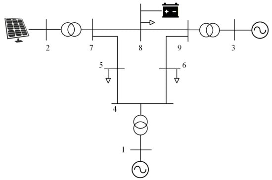
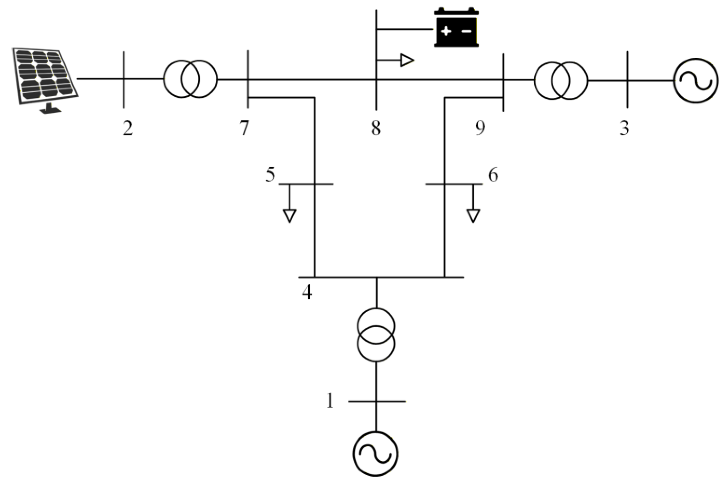
The topology of the WSCC 9-bus system is shown in Figure 13. In this study, Bus 1 is selected as the slack bus to maintain system power balance. A PV is connected to Bus 2 to represent renewable-energy integration, while a BESS is installed at Bus 8, as this bus has comparable electrical distances to both generator buses and load buses within the WSCC 9-bus system. All generator, load, and line parameters follow the standard WSCC 9-bus system settings. The system base capacity is set to 10 MVA, and base voltage is 12.66 kV. The capacity of PV power stations is 12 MW. Programming was performed using MATLAB R2022b on a computer equipped with an Intel i5-12400F processor and 32 GB of RAM, and power flow calculations were carried out using the MATPOWER 8.0 toolbox.

Figure 13. The topology of the WSCC 9-bus system.

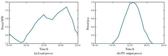
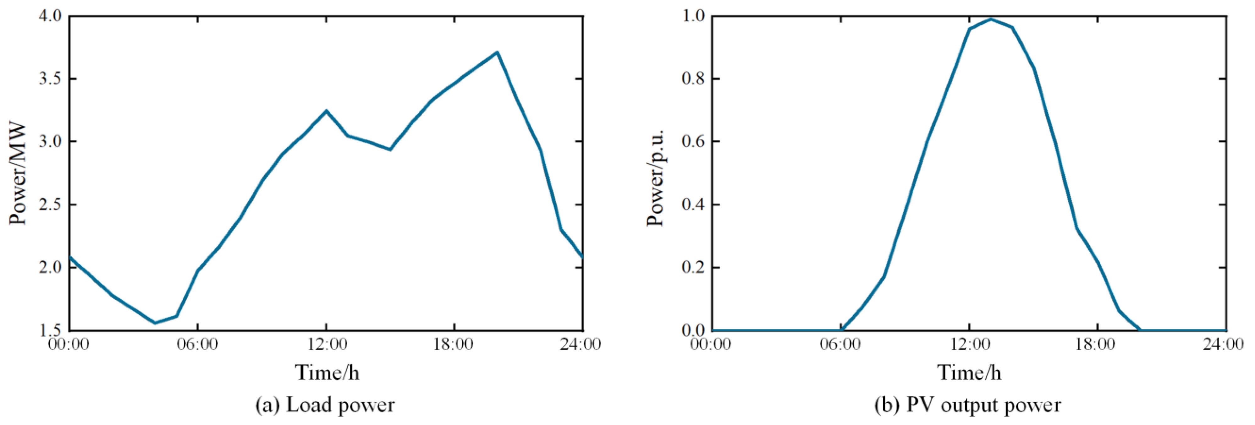
The typical daily load curve and PV output curve are shown in Figure 14a and Figure 14b, respectively.

Figure 14. Load power and PV power curves.

In this study, PV penetration rate is defined as the ratio of the total PV output to the total load in a day:

$$\mathrm{PR}={\displaystyle \frac{{\displaystyle \sum _{\mathrm{t}=1}^{24}{P}_{\mathrm{PV}}(\mathrm{t})}}{{\displaystyle \sum _{\mathrm{t}=1}^{24}{\displaystyle \sum _{\mathrm{n}=1}^9{P}_{\mathrm{load},\mathrm{n}}(\mathrm{t})}}}}$$

(39)

where PR denotes the penetration rate of PV.

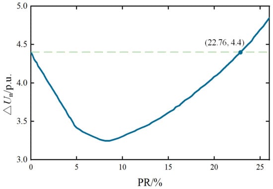
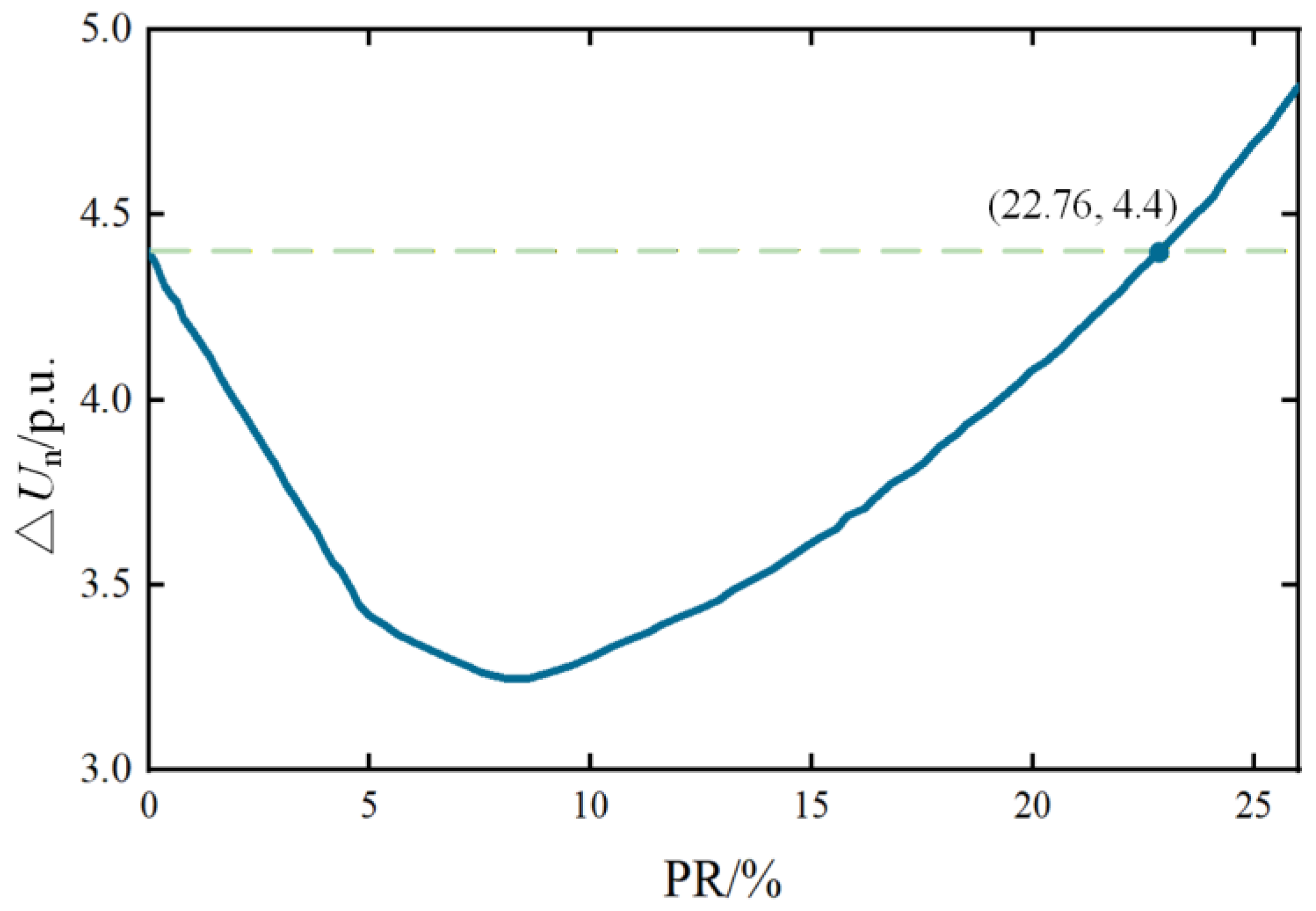
The objective function (36) is used to calculate the degree of voltage fluctuation. By varying the PR in the system and evaluating Equation (36), the corresponding results are shown in Figure 15. As illustrated in Figure 15, when the PR is relatively low, the system voltage fluctuation decreases with increasing PR. This is because, under high-load conditions, higher PV output reduces voltage drops at the nodes. However, as PR continues to increase beyond 8.9%, the node voltages rise, leading to an increase in voltage fluctuations. When PR reaches 22.76%, the voltage fluctuation becomes larger than that of the system without PV integration. Therefore, it is feasible to mitigate voltage fluctuation through the rational configuration of the BESS.

Figure 15. Voltage fluctuation varying with PR.

To verify the feasibility of the proposed model, the PR is set to 26.2%. The maximum number of algorithm iterations is set to 100. The following three scenarios are tested:

Scenario 1: WSCC 9-bus system without PV and BESS;

Scenario 2: WSCC 9-bus system with PV;

Scenario 3: WSCC 9-bus system with PV and BESS, using the MOPSO–TOPSIS framework to solve the problem.

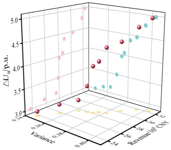
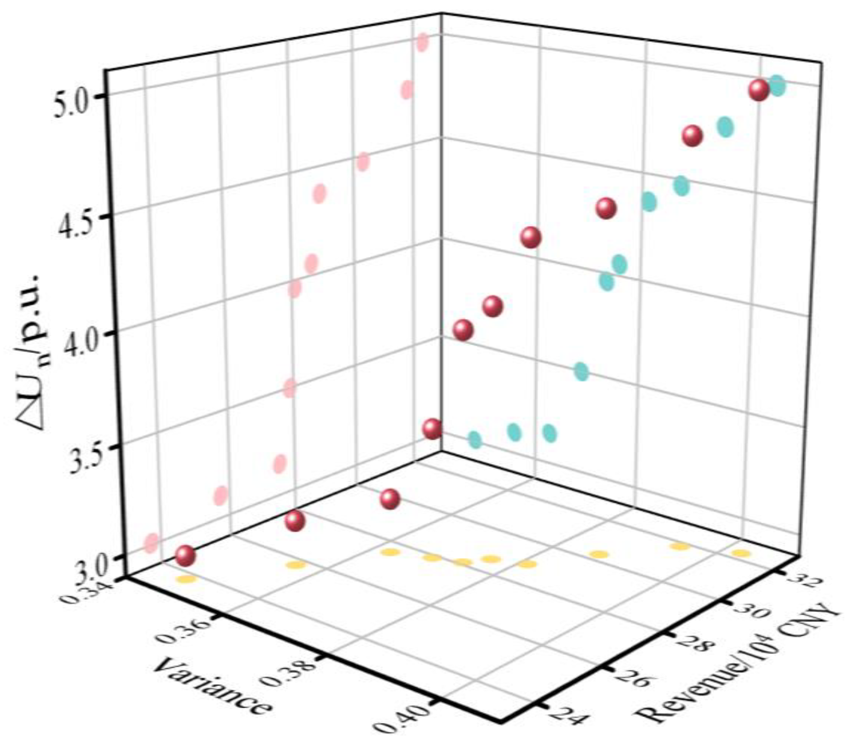
The obtained Pareto frontier is shown in Figure 16. The results for the three scenarios are listed in Table 11.

Figure 16. Pareto frontier under WSCC 9-bus system study.

Table 11. Simulation results under three scenarios.

Scenario	Rated Power (MW)	Rated Capacity (MWh)	∆Un(p.u.)	Revenue (104 CNY)	Variance
1	/	/	4.43	/	0.4028
2	/	/	4.97	/	0.4533
3	6.7	13.3	3.15	27.53	0.3629

In Table 11, a comparison between Scenario 1 and Scenario 2 shows that voltage support is provided after distributed PV integration. However, node voltage fluctuations are increased during PV generation peaks. A comparison between Scenario 2 and Scenario 3 shows that, after BESS integration, node voltage fluctuations are effectively reduced. The voltage fluctuation is reduced by 36.6%.

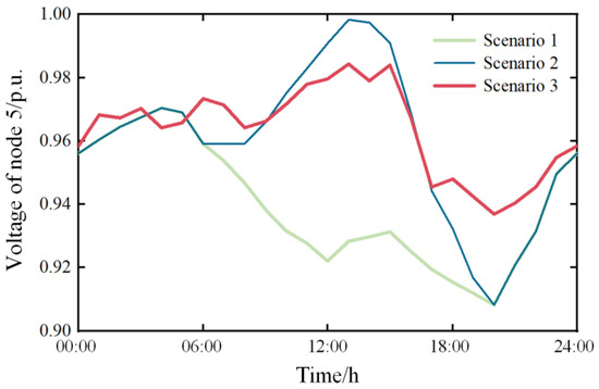
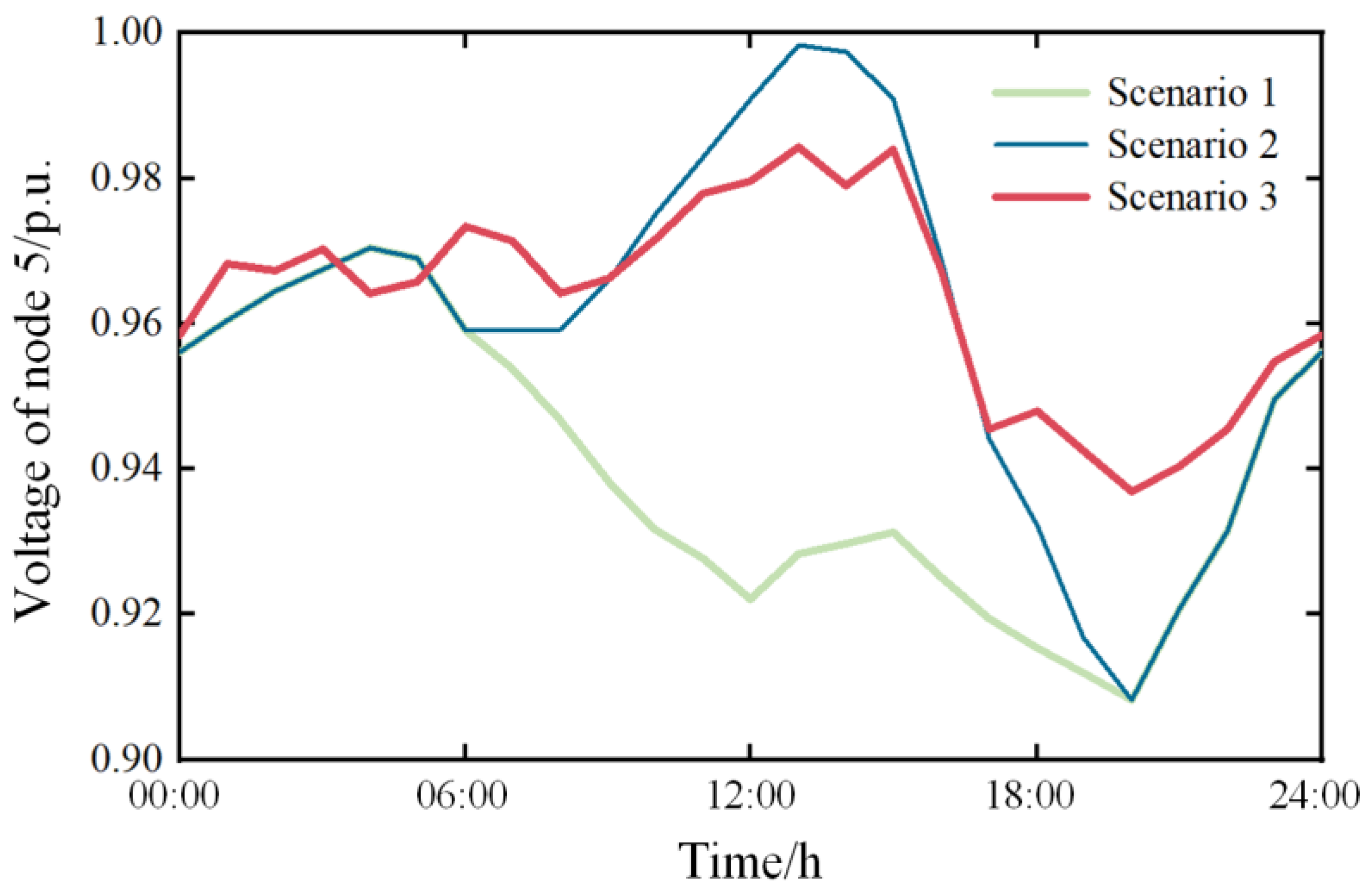
The voltage of node 5 over one day under the three scenarios is shown in Figure 17. A comparison between Scenario 1 and Scenario 2 shows that voltage fluctuations are reduced when PV output is low. As PV output increases, voltage fluctuations are intensified. A comparison between Scenario 2 and Scenario 3 shows that voltage fluctuations are effectively reduced after BESS installation. This result is consistent with the above analysis.

Figure 17. Voltage of node 5.

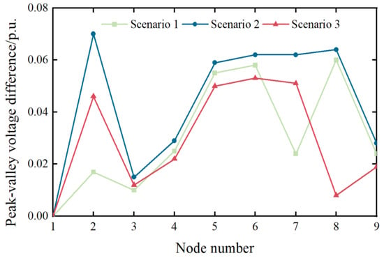
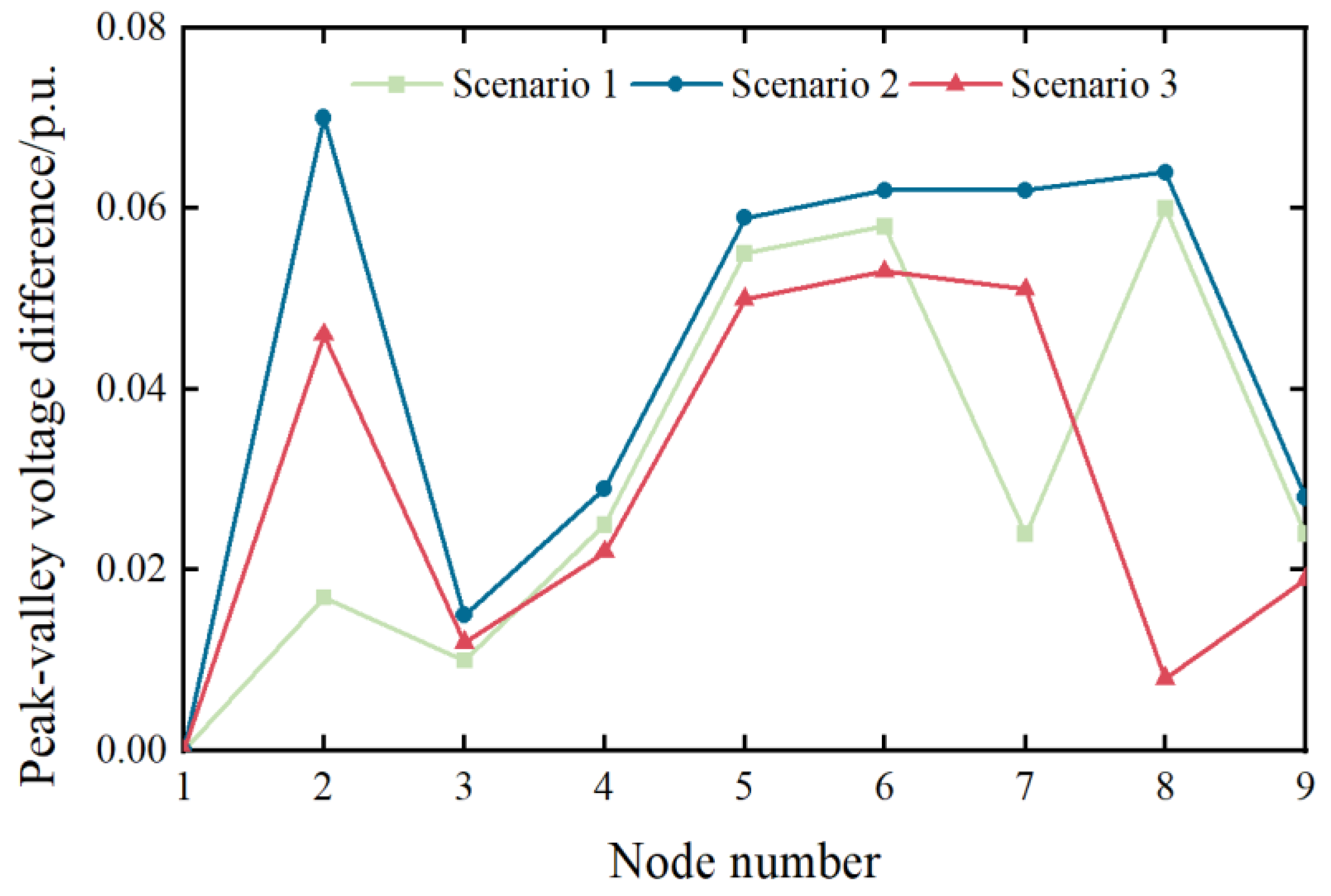
The peak–valley voltage difference over one day under the three scenarios is shown in Figure 18. A comparison between Scenario 1 and Scenario 2 shows that the peak–valley voltage difference is increased after PV installation. This occurs because node voltages rise toward peak values as PR increases. During evening load peaks, PV output is absent. As a result, the peak–valley voltage difference is enlarged.

Figure 18. Peak–valley voltage difference under three scenarios.

A comparison between Scenario 2 and Scenario 3 shows that, after BESS integration, charging occurs during PV generation peaks and discharging occurs during evening load peaks. The peak–valley voltage difference is effectively reduced. The effectiveness of the proposed BESS configuration method is thus validated.

6. Conclusions

This paper proposes a multi-objective optimization framework for the optimal configuration of BESSs in peak shaving and valley filling scenarios. The framework simultaneously considers economic performance and technical effectiveness by maximizing annual revenue and minimizing load variance. A hybrid MOPSO–TOPSIS approach is employed to obtain the Pareto-optimal solution set and select the final configuration. The feasibility and applicability of the proposed method are validated through a typical daily load case study and further extended to a WSCC nine-bus system with PV integration, in which node voltage fluctuation is introduced as an additional system-level objective. Based on the simulation results, the following conclusions can be drawn:

• The proposed framework achieves an effective balance between economic benefits and peak shaving performance. For the typical daily load scenario, the optimal BESS configuration is determined as 27.7 MW/78.3 MWh. With this configuration, the load variance is reduced by 32.15%, and the peak load is reduced by 13.5%, while an average annual revenue of approximately 5.73 million CNY is achieved. These results verify that the proposed framework can identify economically viable configurations while maintaining satisfactory peak shaving and valley filling performance.
• The proposed MOPSO–TOPSIS framework demonstrates superior solution quality and robustness compared with conventional multi-objective solution approaches. Compared with the weighted-sum method, the proposed framework avoids sensitivity to predefined weights and provides configurations with improved economic and technical performance. Furthermore, comparative analysis with the NSGA-II algorithm shows that MOPSO yields a more uniformly distributed Pareto solution set, a wider solution spread, and faster convergence. These results confirm the suitability of the selected algorithm for BESS capacity planning problems and enhance the methodological rigor of the proposed approach.
• The framework exhibits good scalability when extended to networked systems with renewable-energy integration. In the WSCC nine-bus system with PV penetration, the optimized BESS configuration significantly reduces node voltage fluctuations and peak–valley voltage differences. This demonstrates that the proposed framework is not limited to load-level peak shaving applications and can be effectively applied to distribution networks with renewable-energy-induced variability.

Despite the above contributions, several limitations of this study should be acknowledged. First, battery aging is represented using planning-level lifetime parameters without explicitly modeling nonlinear degradation dynamics caused by high-frequency cycling or temperature-dependent electrochemical behavior. Second, thermal constraints are not independently formulated; instead, operational limits are indirectly bounded through rated power and SOC constraints, which may not fully capture real-world thermal management requirements under intensive operation. Third, regulatory and market factors, such as dynamic tariff structures, ancillary service market rules, or policy uncertainty, are simplified as static economic parameters.

Therefore, the proposed framework primarily reflects a configuration-oriented planning perspective rather than a detailed electro-thermal or market-coupled operational model. While this abstraction improves computational tractability and methodological clarity, incorporating physics-based aging models, thermal constraints, and adaptive regulatory mechanisms would further enhance the practical applicability of the framework.

Appendix A.1

Table A1. Normalized matrix Z.

Normalized Value	1	2	3	4	5	6	7
Variance	0.213012552	0.211823368	0.210647388	0.209484393	0.20833417	0.204958059	0.203856874
Revenue	0.159786569	0.169157871	0.175702045	0.180735245	0.184825964	0.193870341	0.196211127
Normalized Value	8	9	10	11	12	13	14
Variance	0.201689625	0.199567972	0.197490492	0.195455818	0.192481221	0.190547951	0.187719781
Revenue	0.200254557	0.203667107	0.206619331	0.209220784	0.212622282	0.214628164	0.217329922

Table A1. Normalized matrix Z.

Normalized Value	1	2	3	4	5	6	7
Variance	0.213012552	0.211823368	0.210647388	0.209484393	0.20833417	0.204958059	0.203856874
Revenue	0.159786569	0.169157871	0.175702045	0.180735245	0.184825964	0.193870341	0.196211127
Normalized Value	8	9	10	11	12	13	14
Variance	0.201689625	0.199567972	0.197490492	0.195455818	0.192481221	0.190547951	0.187719781
Revenue	0.200254557	0.203667107	0.206619331	0.209220784	0.212622282	0.214628164	0.217329922

Appendix A.2

Table A2. Distance to the positive ideal solution and the negative ideal solution.

Distance	1	2	3	4	5	6	7
d+	0.057543353	0.048186727	0.041695014	0.036764362	0.032838918	0.024803766	0.023018036
d−	0.025292771	0.025861249	0.027910169	0.030208366	0.032433383	0.038195048	0.039839104
Distance	8	9	10	11	12	13	14
d+	0.020488454	0.019168443	0.018858714	0.019339002	0.021064126	0.022626484	0.025292771
d−	0.042811384	0.045451967	0.047841137	0.050035866	0.053049825	0.054914471	0.057543353

Table A2. Distance to the positive ideal solution and the negative ideal solution.

Distance	1	2	3	4	5	6	7
d+	0.057543353	0.048186727	0.041695014	0.036764362	0.032838918	0.024803766	0.023018036
d−	0.025292771	0.025861249	0.027910169	0.030208366	0.032433383	0.038195048	0.039839104
Distance	8	9	10	11	12	13	14
d+	0.020488454	0.019168443	0.018858714	0.019339002	0.021064126	0.022626484	0.025292771
d−	0.042811384	0.045451967	0.047841137	0.050035866	0.053049825	0.054914471	0.057543353

Appendix A.3

Table A3. Closeness coefficient.

	1	2	3	4	5	6	7
S	0.305335032	0.349249908	0.400978314	0.451054738	0.496893515	0.606282017	0.633803958
	8	9	10	11	12	13	14
S	0.676326911	0.70336859	0.717260025	0.721239082	0.715787301	0.708199571	0.694664968

Table A3. Closeness coefficient.

	1	2	3	4	5	6	7
S	0.305335032	0.349249908	0.400978314	0.451054738	0.496893515	0.606282017	0.633803958
	8	9	10	11	12	13	14
S	0.676326911	0.70336859	0.717260025	0.721239082	0.715787301	0.708199571	0.694664968

References

- Golmohamadi, H. Demand-Side Management in Industrial Sector: A Review of Heavy Industries. Renew. Sustain. Energy Rev. 2022, 156, 111963. [Google Scholar] [CrossRef] [Scilit]
- Ku, T.-T.; Li, C.-S. Implementation of Battery Energy Storage System for an Island Microgrid with High PV Penetration. IEEE Trans. Ind. Appl. 2021, 57, 3416–3424. [Google Scholar] [CrossRef] [Scilit]
- Gu, Y.; Xu, J.; Chen, D.; Wang, Z.; Li, Q. Overall Review of Peak Shaving for Coal-Fired Power Units in China. Renew. Sustain. Energy Rev. 2016, 54, 723–731. [Google Scholar] [CrossRef] [Scilit]
- Jafarizadeh, H.; Yamini, E.; Zolfaghari, S.M.; Esmaeilion, F.; Assad, M.E.H.; Soltani, M. Navigating Challenges in Large-Scale Renewable Energy Storage: Barriers, Solutions, and Innovations. Energy Rep. 2024, 12, 2179–2192. [Google Scholar] [CrossRef] [Scilit]
- Jaradat, T.; Khatib, T. A Review of Battery Energy Storage System for Renewable Energy Penetration in Electrical Power System: Environmental Impact, Sizing Methods, Market Features, and Policy Frameworks. Future Batter. 2025, 7, 100106. [Google Scholar] [CrossRef] [Scilit]
- Wu, T.; Zhang, Y.J.; Tang, X. A VSC-Based BESS Model for Multi-Objective OPF Using Mixed Integer SOCP. IEEE Trans. Power Syst. 2019, 34, 2541–2552. [Google Scholar] [CrossRef] [Scilit]
- Chatzigeorgiou, N.G.; Theocharides, S.; Makrides, G.; Georghiou, G.E. A Review on Battery Energy Storage Systems: Applications, Developments, and Research Trends of Hybrid Installations in the End-User Sector. J. Energy Storage 2024, 86, 111192. [Google Scholar] [CrossRef] [Scilit]
- Jaradat, T.; Khatib, T. Optimal Sizing of Battery Energy Storage System in Electrical Power Distribution Network. Energy Explor. Exploit. 2025, 43, 909–931. [Google Scholar] [CrossRef] [Scilit]
- Vaka, S.S.K.R.; Matam, S.K. Optimal Sizing and Management of Battery Energy Storage Systems in Microgrids for Operating Cost Minimization. Electr. Power Compon. Syst. 2021, 49, 1319–1332. [Google Scholar] [CrossRef] [Scilit]
- Zhang, Y.; Xu, Y.; Yang, H.; Dong, Z.Y.; Zhang, R. Optimal Whole-Life-Cycle Planning of Battery Energy Storage for Multi-Functional Services in Power Systems. IEEE Trans. Sustain. Energy 2020, 11, 2077–2086. [Google Scholar] [CrossRef] [Scilit]
- High-Dimensional Multi-Objective Bayesian Optimization with Block Coordinate Updates: Case Studies in Intelligent Transportation System. Available online: https://ieeexplore.ieee.org/document/10040106 (accessed on 22 November 2025).
- Ruvio, A.; Dell’Olmo, J.; Maccioni, M.; Nati, L.; Bragatto, T. MILP Based Optimization Tool for PV and BESS Planning in Railways: A Case Study in Extensive Market Analysis. Sustain. Energy Grids Netw. 2025, 44, 102063. [Google Scholar] [CrossRef] [Scilit]
- Moser, M.; Gils, H.-C.; Pivaro, G. A Sensitivity Analysis on Large-Scale Electrical Energy Storage Requirements in Europe under Consideration of Innovative Storage Technologies. J. Clean. Prod. 2020, 269, 122261. [Google Scholar] [CrossRef] [Scilit]
- Li, Y.; Xie, Z.; Yang, S.; Ren, Z. A Novel Hybrid Multi-Objective Optimization Algorithm and Its Application to Designs of Electromagnetic Devices. IEEE Trans. Magn. 2025, 61, 7200304. [Google Scholar] [CrossRef] [Scilit]
- Noori, M.S.; Sahbudin, R.K.Z.; Sali, A.; Hashim, F. Multi-Objective Multi-Exemplar Particle Swarm Optimization Algorithm with Local Awareness. IEEE Access 2024, 12, 125809–125834. [Google Scholar] [CrossRef] [Scilit]
- Adar, M.; Babay, M.-A.; Boussif, M.; Khaouch, Z.; Abbassi, Z.; Najih, Y.; Mabrouki, M. Optimization of Photovoltaic System Modelling: A Comparative Study and Experimental Validation Using Bond Graph Methodology and a Genetic Algorithm. In Applied Mathematics, Modeling and Computer Simulation; IOS Press: Amsterdam, The Netherlands, 2024; pp. 723–730. [Google Scholar]
- Li, B.; Roche, R.; Paire, D.; Miraoui, A. Sizing of a Stand-Alone Microgrid Considering Electric Power, Cooling/Heating, Hydrogen Loads and Hydrogen Storage Degradation. Appl. Energy 2017, 205, 1244–1259. [Google Scholar] [CrossRef] [Scilit]
- Hesse, H.C.; Martins, R.; Musilek, P.; Naumann, M.; Cong, N.T.; Jossen, A. Economic Optimization of Component Sizing for Residential Battery Storage Systems. Energies 2017, 10, 835. [Google Scholar] [CrossRef] [Scilit]
- Miranda, I.; Silva, N.; Leite, H. A Holistic Approach to the Integration of Battery Energy Storage Systems in Island Electric Grids with High Wind Penetration. IEEE Trans. Sustain. Energy 2016, 7, 775–785. [Google Scholar] [CrossRef] [Scilit]
- Barzkar, A.; Hosseini, S.M.H. A Novel Peak Load Shaving Algorithm via Real-Time Battery Scheduling for Residential Distributed Energy Storage Systems. Int. J. Energy Res. 2018, 42, 2400–2416. [Google Scholar] [CrossRef] [Scilit]
- Tan, Y.; Wen, M.; Liao, J.; Wang, C.; Liu, Y.; Ouyang, T. Scheduling Strategy of Energy Storage Peak-Shaving and Valley-Filling Considering the Improvement Target of Peak-Valley Difference. In Proceedings of the 2021 11th International Conference on Power and Energy Systems (ICPES), Shanghai, China, 18–20 December 2021; pp. 196–200. [Google Scholar]
- Cheng, C.; Su, C.; Wang, P.; Shen, J.; Lu, J.; Wu, X. An MILP-Based Model for Short-Term Peak Shaving Operation of Pumped-Storage Hydropower Plants Serving Multiple Power Grids. Energy 2018, 163, 722–733. [Google Scholar] [CrossRef] [Scilit]
- Liu, J.; Wang, H.; Du, Y.; Lu, Y.; Wang, Z. Multi-Objective Optimal Peak Load Shaving Strategy Using Coordinated Scheduling of EVs and BESS with Adoption of MORBHPSO. J. Energy Storage 2023, 64, 107121. [Google Scholar] [CrossRef] [Scilit]
- Wang, Y.; Duan, J.; Li, Z.; Xiao, X.; Zhou, X.; Yang, H.; Yang, J. Optimal Energy Storage Configuration for Power Quality Enhancement in Active Distribution Networks with Coordinated PV Operation. Int. J. Electr. Power Energy Syst. 2025, 172, 111225. [Google Scholar] [CrossRef] [Scilit]
- He, S.; Wu, P.; Li, X.; Bo, Y.; Yun, P. Adaptive Modified Unbiased Minimum-Variance Estimation for Highly Maneuvering Target Tracking with Model Mismatch. IEEE Trans. Instrum. Meas. 2023, 72, 8501216. [Google Scholar] [CrossRef] [Scilit]
- Luan, Z.; Zhao, W.; Wang, C. Research on Variable Time-Scale SOC and SOH Asynchronous Collaborative Estimation Strategy for Electric Vehicle Power Lithium Iron Phosphate Batteries. J. Energy Storage 2023, 73, 108826. [Google Scholar] [CrossRef] [Scilit]
- Cao, Y.; Wu, Q.; Zhang, H.; Li, C.; Zhang, X. Chance-Constrained Optimal Configuration of BESS Considering Uncertain Power Fluctuation and Frequency Deviation Under Contingency. IEEE Trans. Sustain. Energy 2022, 13, 2291–2303. [Google Scholar] [CrossRef] [Scilit]
- Apribowo, C.H.B.; Hadi, S.P.; Danang Wijaya, F.; Setyonegoro, M.I.B.; Sarjiya. Optimal Sizing and Placement of Battery Energy Storage System for Maximum Variable Renewable Energy Penetration Considering Demand Response Flexibility: A Case in Lombok Power System, Indonesia. Energy Convers. Manag. X 2024, 23, 100620. [Google Scholar] [CrossRef] [Scilit]
- Zitzler, E.; Deb, K.; Thiele, L. Comparison of Multiobjective Evolutionary Algorithms: Empirical Results. Evol. Comput. 2000, 8, 173–195. [Google Scholar] [CrossRef] [Scilit] [PubMed]
- Cai, J.; Wang, K.; Cheok, A.D.; Yan, Y. Optimal Configuration for Power Grid Battery Energy Storage Systems Based on Payload Fluctuation Guided Multi-Objective PSO. J. Energy Storage 2025, 105, 114515. [Google Scholar] [CrossRef] [Scilit]
- Deb, K.; Pratap, A.; Agarwal, S.; Meyarivan, T. A Fast and Elitist Multiobjective Genetic Algorithm: NSGA-II. IEEE Trans. Evol. Comput. 2002, 6, 182–197. [Google Scholar] [CrossRef] [Scilit]
- Lu, L.; Chu, G.; Zhang, T.; Yang, Z. Optimal configuration of energy storage in a microgrid based on improved multi-objective particle swarm optimization. Power Syst. Prot. Control. 2020, 48, 116–124. [Google Scholar] [CrossRef]
Disclaimer/Publisher’s Note: The statements, opinions and data contained in all publications are solely those of the individual author(s) and contributor(s) and not of MDPI and/or the editor(s). MDPI and/or the editor(s) disclaim responsibility for any injury to people or property resulting from any ideas, methods, instructions or products referred to in the content. |
© 2026 by the authors. Licensee MDPI, Basel, Switzerland. This article is an open access article distributed under the terms and conditions of the Creative Commons Attribution (CC BY) license.