


Abstract
Microseismic identification and localization of signals from single-component distributed optical fiber acoustic sensors (DAS) in vertical wells are limited by low signal-to-noise ratio and lack of directional information, making effective signal identification and accurate localization difficult. Improving the detection rate and accuracy of such data events is helpful for analyzing the effect of fracturing. To address this, this paper proposes a method for automatically picking and locating microseismic events based on dual fitting modeling and waveform inversion. First, empirical mode decomposition (EMD) is used to adaptively decompose and reconstruct the original DAS signal to filter out approximately 80% of high-frequency noise (noise above 200 Hz). Second, the classic short-time average/long-time average energy ratio algorithm is used to pick all “event points.” Finally, DBSCAN density clustering and RANSAC robust fitting are combined to perform secondary screening and fitting modeling of the “event points” to obtain the continuous event arrival time distribution along the well section direction, and the spatial location of the seismic source is inverted based on the fitting results. Tested with experimental data from Well XX, the automatic detection rate reached 96%, and the accuracy of machine detection compared with manual judgment reached 95%.
1. Introduction
Real-time monitoring of reservoir stimulation effects and fracture propagation characteristics is crucial for optimizing oil and gas operations, enhancing production capacity, and controlling costs in the development of unconventional oil and gas fields. The hydraulic fracturing technology uses high-pressure pumping of fluids to specifically break the rocks and utilizes the support materials to maintain the conductivity of the fractures. Meanwhile, on-site personnel monitor the geometric shape and sweep range of the fracture network in real time. Based on the dynamic feedback of fracture expansion, they promptly adjust the pumping rate, liquid viscosity, and sand addition procedures, thereby achieving precise optimization of the construction process. During this process, the increase in the complexity of the fracture network not only significantly increases the contact area between the reservoir and the wellbore, ensuring the smoothness of the oil and gas flow channels, but more importantly, the refined operation based on real-time effect evaluation can effectively avoid the blind investment of materials and ineffective construction [1,2,3]. Microseismic monitoring is a crucial technology for evaluating fracturing impacts due to its ability to provide real-time and spatially precise information on fracture propagation [4,5]. The implementation and efficacy of the sensing system substantially influence the precision of microseismic monitoring, especially in complex downhole environments that may limit the coverage, durability, and deployment expenses of traditional geophone arrays [6,7,8].
In recent years, the development of Distributed Acoustic Sensing (DAS) technology has provided a new solution for microseismic monitoring. As an evolution in the field of sensing, DAS technology has rapidly expanded its application scope from the initial use in long-distance perimeter security and fiber optic communication link monitoring to oil and gas resource development, urban underground space imaging, and earthquake early warning. Based on the principle of coherent Rayleigh scattering, this technology enables high-density and continuous distributed signal acquisition along the well section. Moreover, due to its advantages such as high temperature and high pressure resistance, anti-interference, and long-term monitoring, it demonstrates significant application potential in dynamic monitoring of oil and gas reservoirs [9,10]. Nonetheless, the implementation of DAS in vertical wells continues to encounter obstacles. The signal obtained from optical fibers consists solely of single-component data along the wellbore axis, and the absence of directionality constrains the precision of event identification and source localization [11]. Furthermore, the diminished signal-to-noise ratio and intricate background noise substantially elevate the challenges associated with data processing [12]. This paper presents a methodology for the automated detection and localization of microseismic events utilizing dual fitting modeling and waveform inversion, specifically for identifying and locating single-component DAS data in vertical wells, thereby offering insights for the engineering application of DAS technology in vertical well microseismic monitoring.
This paper initially presents a preprocessing and event identification methodology for DAS data, significantly enhancing the detection rate of low signal-to-noise ratio events. A time-based selection technique for fitting and localization is developed using data processing. Ultimately, application verification is performed with field data, illustrating the viability and efficacy of this approach in practical engineering. The research findings offer a novel methodological framework for the utilization of DAS technology in microseismic monitoring and suggest potential for its extensive application in unconventional oil and gas development, facilitating cost reduction, efficiency enhancement, and resource optimization within the industry.
2. Data Processing
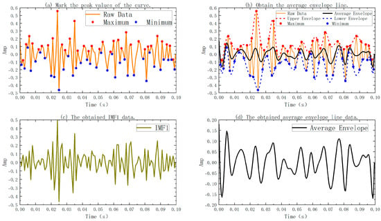
During the application of DAS technology for microseismic monitoring and signal analysis, the raw data frequently encounters numerous influences, including intricate geological conditions, ambient environmental noise, and instrument response, resulting in attributes such as non-stationarity, nonlinearity, low signal-to-noise ratio, and signal amalgamation [13,14]. Specifically, due to the high-frequency vibrations of the on-site pumping units, the pulsating flow of pipes, and the interference from surrounding vehicles, these often highly overlap with the weak microseismic signals in the time-frequency domain. Such data is challenging to efficiently segregate and extract with conventional linear time-frequency analysis techniques, like Fourier transform or wavelet transform [15,16]. Consequently, this research employs the empirical mode decomposition (EMD) technique. The Fourier transform is limited by the assumption of global stationarity and is unable to effectively depict the transient sudden change characteristics of microseismic events. Although the wavelet transform has the ability of time-frequency localization, its decomposition effect highly depends on the preset wavelet basis functions, and it is difficult to truly fit the time-varying mixed noise formed by complex environmental interference and system responses in the original DAS data. In contrast, EMD abandons the constraint of priori basis functions and separates signals with different central frequencies, extracting specific signals by frequency screening. It is particularly suitable for processing non-stationary microseismic sequences under high background noise. The specific implementation of EMD is based on the local characteristics of the signal itself. Through an iterative screening process, it gradually extracts oscillation components at different time scales to achieve adaptive decomposition of the signal [17,18]. In the following, I will introduce the relevant principle of EMD signal decomposition through Figure 1.
Figure 1.
Stepwise EMD sifting process illustration.
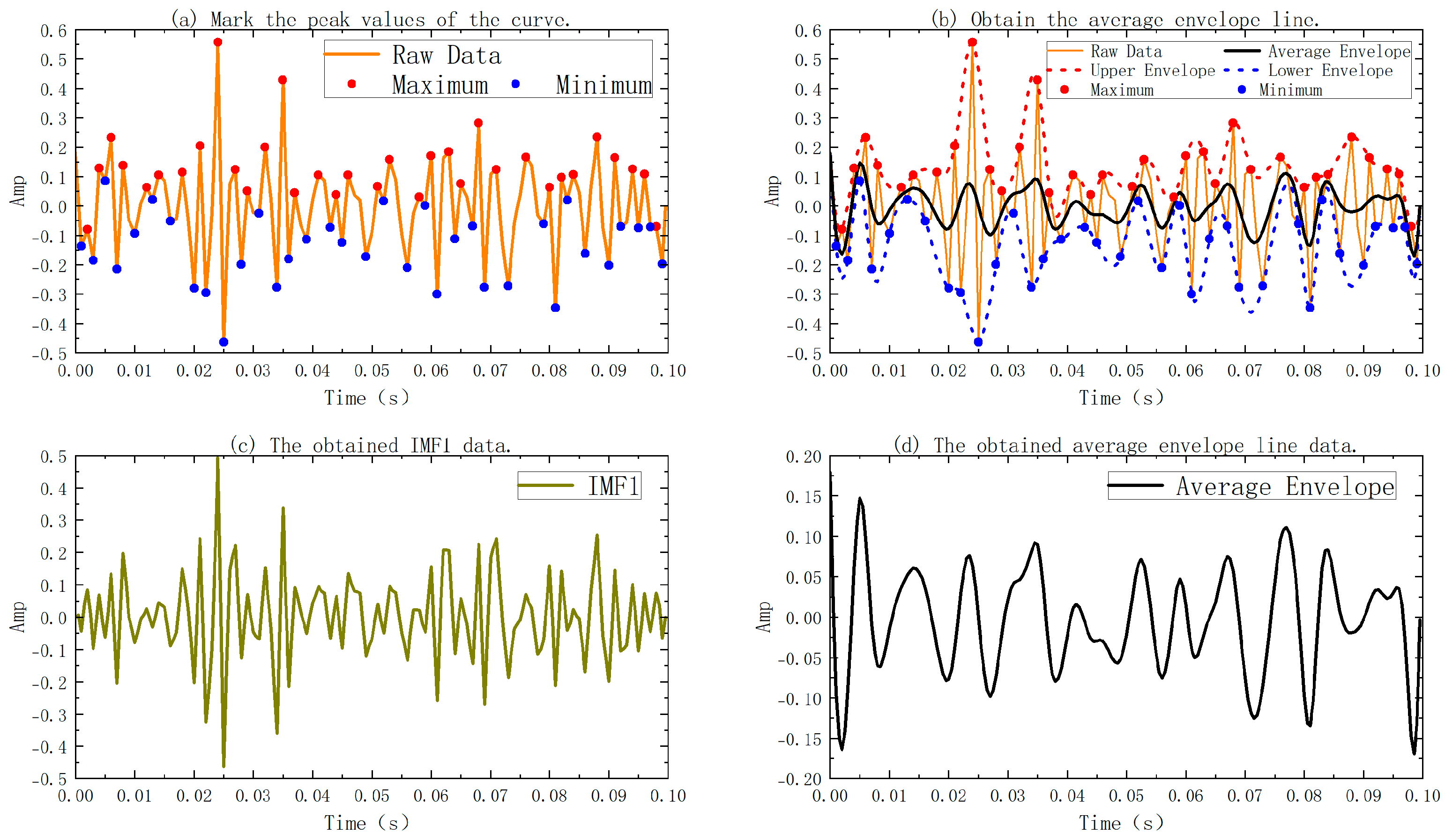
In Figure 1, Figure 1a shows the original signal to be detected; Figure 1b shows the upper envelope, lower envelope, and average envelope plotted on the curve of the original signal; Figure 1c shows the IMF1 obtained after subtracting the average envelope from the original signal; the average envelope in Figure 1d is also a new function obtained after filtering out one high-frequency signal. Figure 1 depicts the decomposition process and the evolution of signal features of the original DAS signal utilizing the EMD approach. Figure 1a illustrates that the original signal has considerable non-stationarity and multi-scale oscillatory properties in the temporal domain, encompassing both high-frequency noise components and overlaid mid-to-low-frequency responses resulting from seismic occurrences. All local maxima and minima of the signal are delineated in the curve presented in Figure 1a. Upper and lower envelopes are generated using cubic spline interpolation of these extreme locations. The average of the higher and lower envelopes is utilized to generate a new signal that filters out approximately 80% of the high-frequency characteristics, as illustrated in Figure 1b. The new signal is recovered from the original signal, uncovering Intrinsic Mode Functions (IMFs) that meet the criterion of having a comparable amount of local extrema and zeros. If the relationship between extrema and zeros is not fulfilled, the aforementioned process is reiterated until the termination criterion is achieved (the disparity between the number of extrema and zeros is less than or equal to 1, and the signal mean is 0 or a negligible value close to 0). This procedure will produce a sequence of IMFs, wherein the high-frequency rapid oscillations are initially isolated, followed by the separation of mid- and low-frequency components through successive iterations.
3. Microseismic First-Arrival Picking
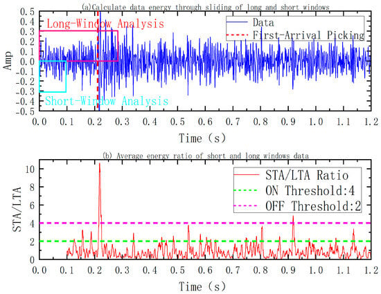
Following the completion of EMD and signal reconstruction, event detection and arrival time identification are necessary for the augmented DAS signal to facilitate further waveform fitting and source location. This study employs the traditional Short-Term Average to Long-Term Average (STA/LTA) technique for preliminary selection [19,20,21]. Figure 2 below is a simple illustration of the STA/LTA method.
Figure 2.
STA/LTA triggering mechanism illustration.
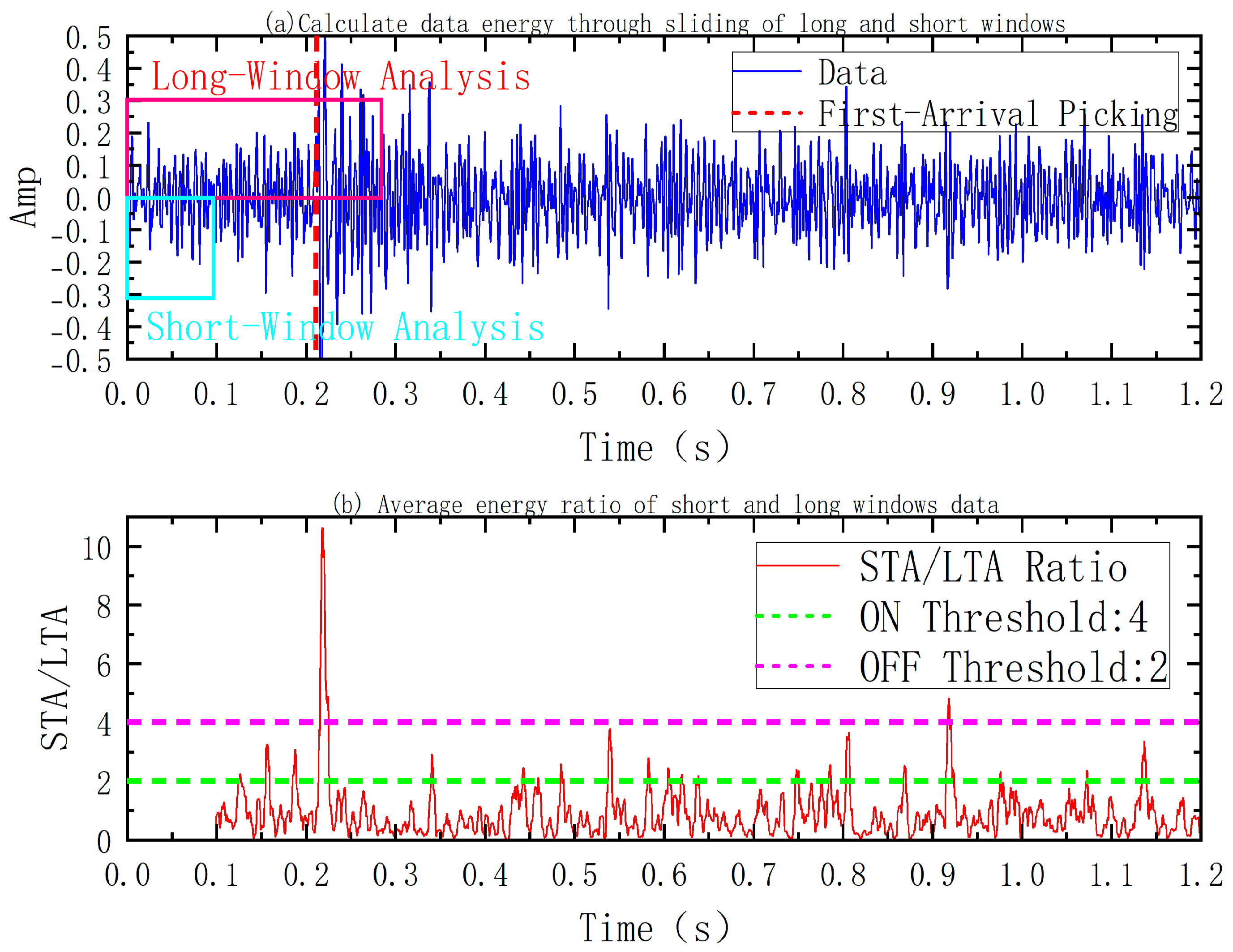
In Figure 2, the original DAS signal manifests as a continuous waveform sequence in the time domain, exhibiting a notable rise in amplitude fluctuations near the event point. The local average energy of the signal is computed by establishing sliding time windows of varying durations. In Figure 2a, the ratio of the average energy within the short time frame (blue box) to that within the long time window (red box) signifies the occurrence of a quick change in the signal; thus, this average energy ratio serves as an indicator for the presence of a microseismic event. In Figure 2b, the initiation and conclusion of event detection are established by applying an ON Threshold (green dashed line) and an OFF Threshold (red dashed line).
4. Data Fitting and Localization
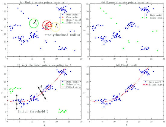
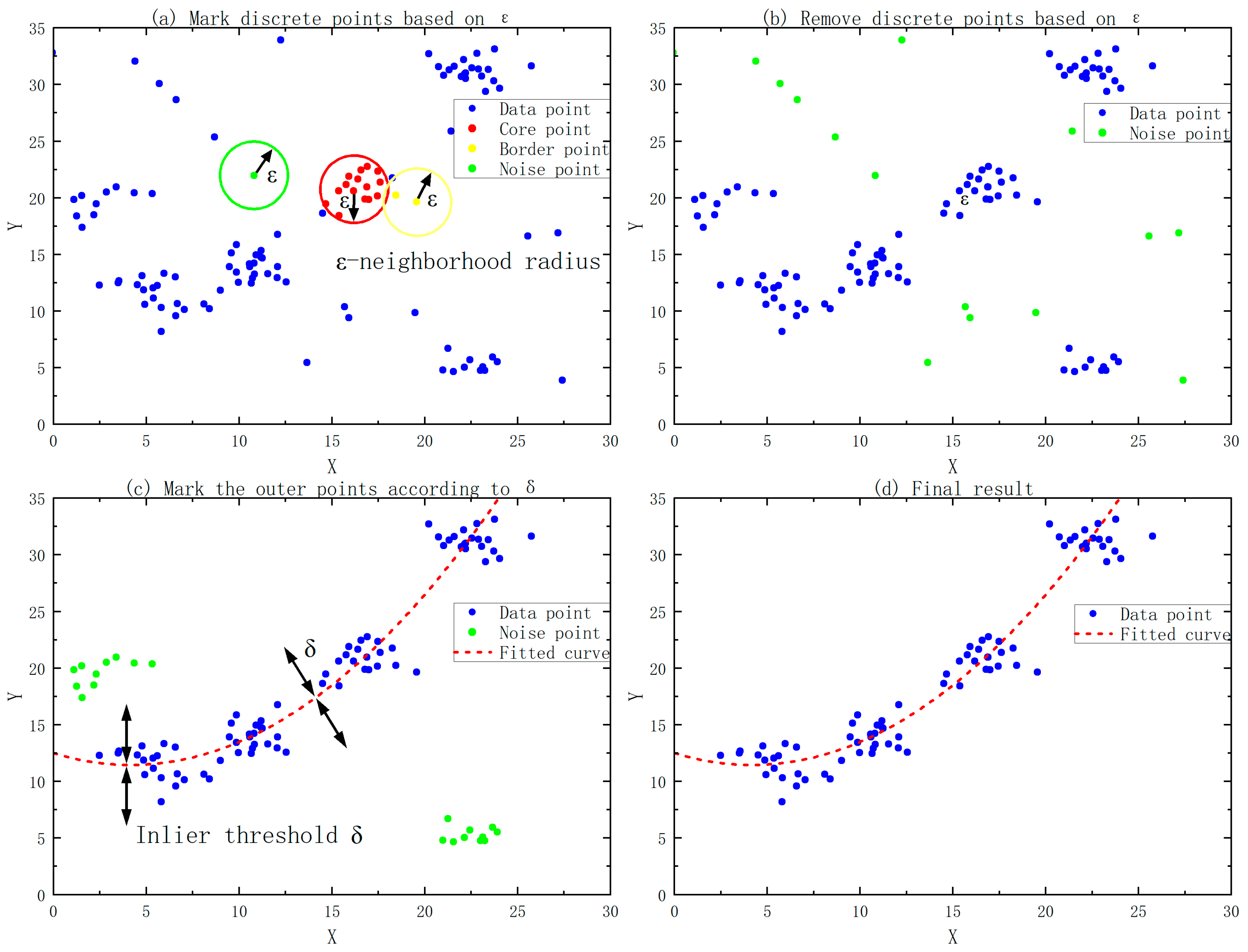
The STA/LTA algorithm is commonly employed for seismic event detection because of its computational efficiency and real-time capabilities; yet, it possesses notable limitations in actual engineering contexts. This is mainly reflected in the assumption that the background noise of the data is stable and the energy of the event signal changes significantly. Despite processing, the DAS signal retains interference, resulting in energy ratio variations even in the absence of events, thus producing several false trigger points. This paper utilizes a data fitting search method that integrates Density-Based Spatial Clustering of Applications with Noise (DBSCAN) clustering analysis and RANSAC (Random Sample Consensus) robust fitting to conduct a secondary screening of the spatial and temporal distribution characteristics of trigger points. Figure 3 shows the process of the DBSCAN clustering algorithm.
Figure 3.
DBSCAN clustering process illustration.
In Figure 3, Figure 3a shows the clustering selection process for all data points; Figure 3b shows the results after selection; Figure 3c shows the selection of interior points with the smallest distance to the fitted function through iterative fitting; and Figure 3d shows the final fitting results after selection. As shown in Figure 3, let the set of trigger points obtained by the STA/LTA algorithm be:
In the above formula, is the trigger time and is the fiber optic channel position.
Calculate the local neighborhood density using the DBSCAN algorithm [22,23]:
In Formula (2), represents the number of other data points within the neighborhood radius that are located around the data point , and is referred to as the number of points within the cluster. If the distance between and is less than ε, then is an internal point of , and the value of is incremented by one. In Figure 3a, we pre-set a neighborhood radius and the minimum number of points MinPts. The values of these parameters are selected empirically based on the number and density of data points in the figure. If the filtered signal after the STA/LTA acquisition has many false triggers, then the neighborhood radius is reduced accordingly, and the number of points within the cluster is increased accordingly to filter out the false triggers. Then, all the data points are automatically classified into three categories according to the relationship between and the minimum number of points MinPts:
1. Core points (A) are the centers of high-density regions containing a sufficient number of samples within their neighborhood;
2. Boundary points (C) do not meet the density condition themselves but are located within the neighborhood of core points;
3. Outliers (N) have low density and are identified as noise points.
This process automatically identifies spatiotemporally continuous real event triggering clusters and marks isolated noise triggering points as outliers and removes them. In actual processing, there may be multiple data clusters. Further optimization and processing can be performed by selecting several large clusters with a large number of data points. After density clustering, to further explore potential patterns in the data, the Random Sample Consensus (RANSAC) algorithm is used for robust model fitting. A small number of data points from randomly sampled data clusters are used to estimate possible function models, and points within the error threshold are identified and considered “inliers”. After continuous iteration, the model with the most inliers is selected as the optimal solution. The final result is shown in Figure 3d. The red dashed line represents the optimal function curve obtained by RANSAC fitting, the blue points are data points that conform to the model, and the orange points that deviate significantly are considered outliers and are removed.
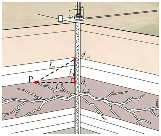
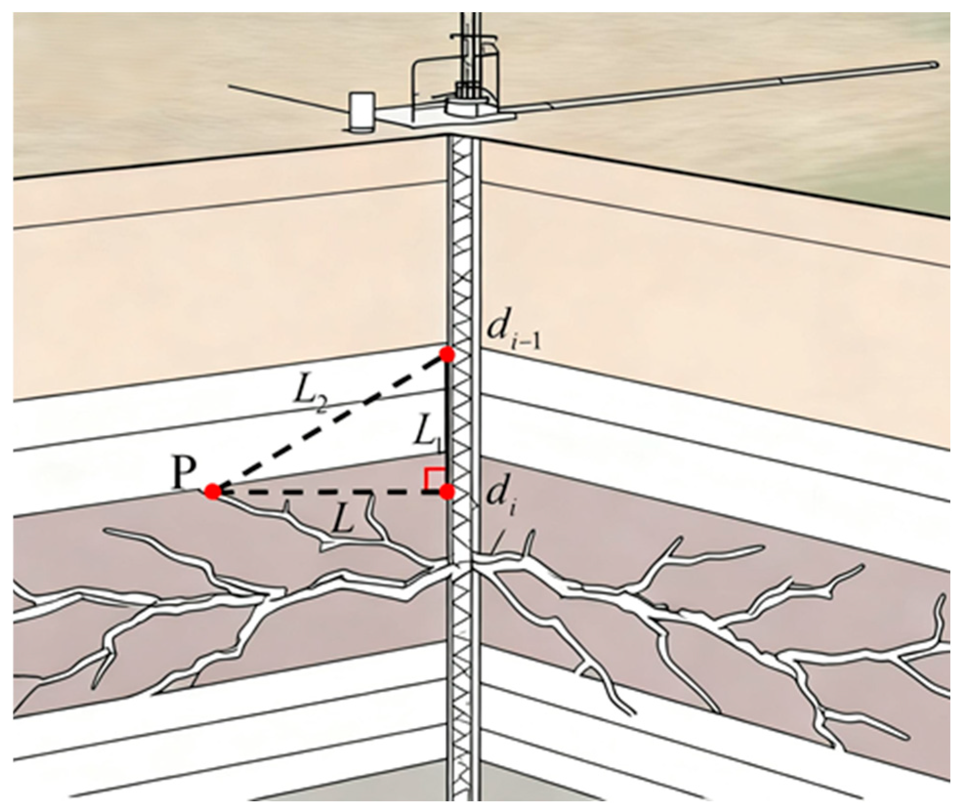
The fitted curve obtained after the above processing can provide the continuous arrival time distribution of the event along the well section. The earliest receiving point on the curve is defined as (ti, di), which represents the channel position closest to the source on the signal propagation path. At the same time, the vertical direction of this point along the vertical well serves as the initial reference for the source azimuth. Figure 4 below presents an abstract two-dimensional illustration of the seismic source determination.
Figure 4.
Epicentral distance calculation illustration.
In Figure 4, it is assumed that the propagation velocity of the microseismic event at point P to channels di and di−1 is v (in this article, it is assumed that the non-uniform strata have no significant effect on the propagation speed of waves), the propagation distances are L and L2, respectively, and the propagation times are t1 and t2, respectively. The fiber optic channel spacing is L1, and the arrival time difference from point P to the adjacent channel can be calculated from the fitted curve as follows:
Finally, by solving a series of equations, we can obtain the vertical position of the final event point in the wellbore direction as follows:
The last unknown component is selected based on the direction of crack extension at the corresponding component at the crack point. In the context of measuring and locating underground micro-earthquake events using a single optical fiber during hydraulic fracturing in engineering, the perforations in the fracturing section are usually only on one side, which is similar to a one-dimensional solution. If there are multiple perforation sides, the micro-earthquake event will have an infinite number of solutions under the condition of a single optical fiber. Therefore, the last component is located towards the perforation side according to the construction report. In the conference report of Luo et al. (2022) [24], the relationship between the micro-earthquake event and the crack was described. If the crack height is below 75 m, the error is less than 10 m. Therefore, it is assumed that the micro-earthquake source is at the position of point P in Figure 4.
5. Results and Discussion
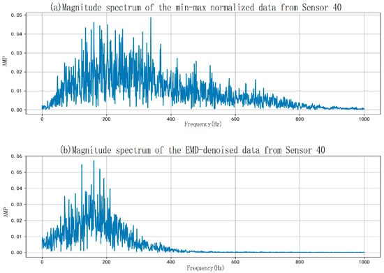
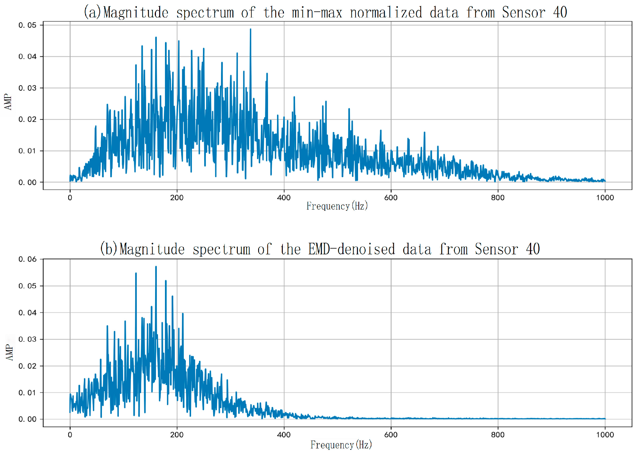
Microseismic monitoring data was tested on Well XX (the names of the wells used as references for the data in the experiment). The system employed a hybrid observation network combining DAS and a three-component seismograph. Each event was recorded for 1.2 s at a sampling rate of 2000 Hz. For the DAS channel, the spatial sampling interval was approximately 2 m, enabling the acquisition of high spatial resolution acoustic responses along the wellbore. Figure 5 below shows the comparison of the 40th channel before and after filtering for Event 100001 of Well XX.
Figure 5.
Comparative waveform analysis of sensor 40 data from well XX: pre- and post-bandpass filtering for event 100001.
Figure 5 shows the denoised data obtained by applying EMD filtering to the standardized data from a single channel of Well XX. It is clear from the figure that almost all high frequencies in the original data are removed after filtering, while low frequencies (data below 200 Hz) are preserved and enhanced to some extent. To quantify the high-frequency removal ratio before and after filtering, the algorithm calculates the high-frequency energy values before and after filtering for data above 200 Hz. The results from multiple sets of data are then averaged to obtain an estimate of the high frequencies removed after denoising. The table shows that the EMD filtering algorithm can remove approximately 80% of the high-frequency signals from the original signal. The following presents the relevant content of the experimental results as shown in Table 1, Figure 6 and Figure 7. In Table 1, the average values obtained from multiple measurements are used for comparison for each event.
Table 1.
Comparative energy analysis of microseismic events across sensor array: pre- vs. post-denoising radiated energy.
Figure 6.
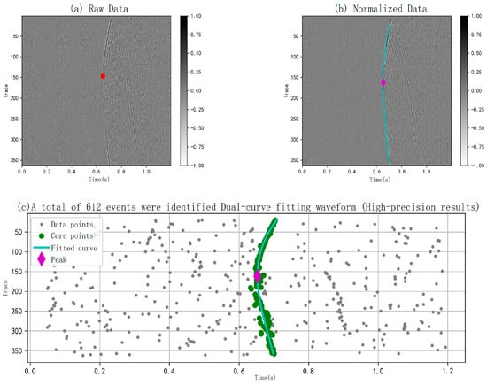
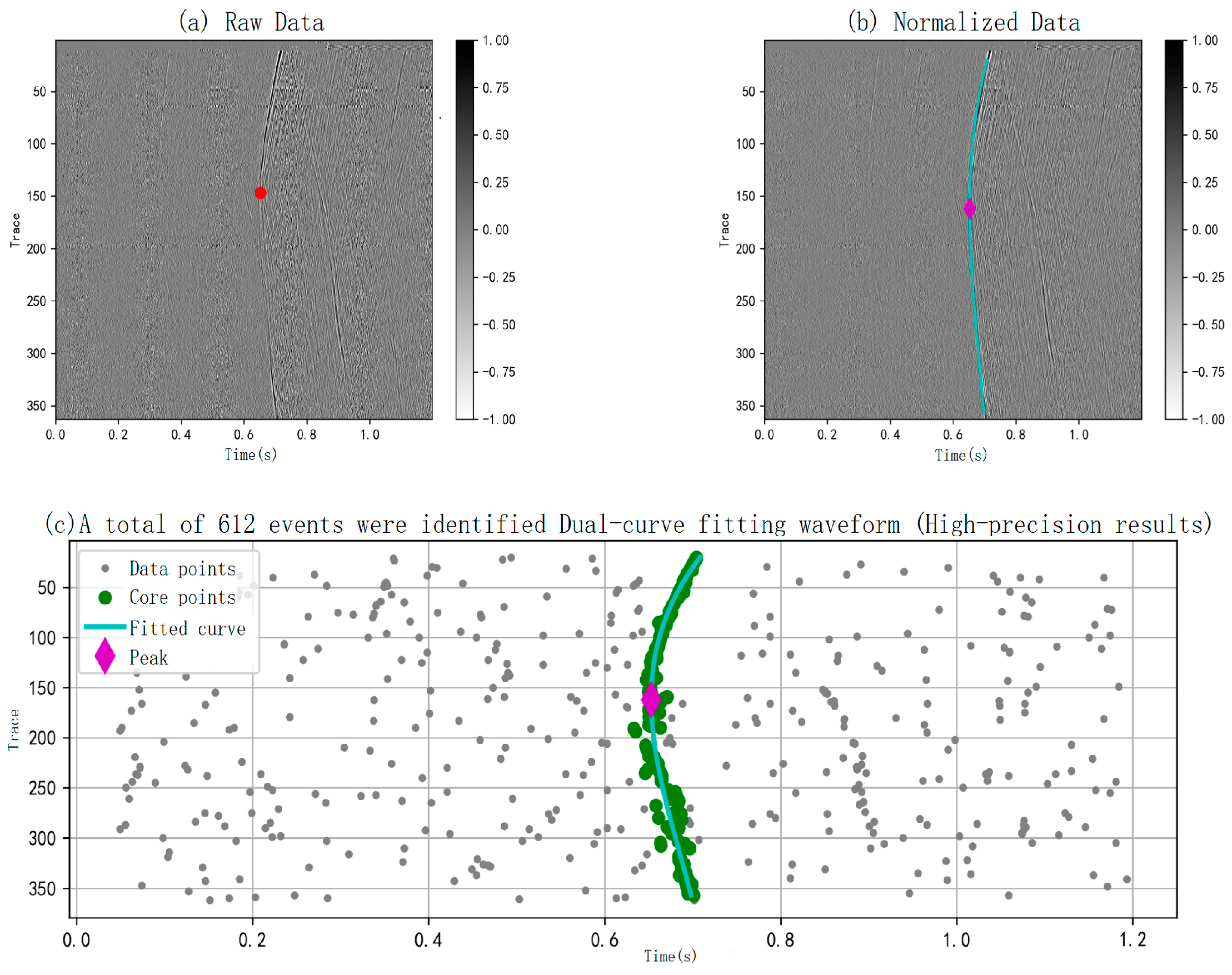
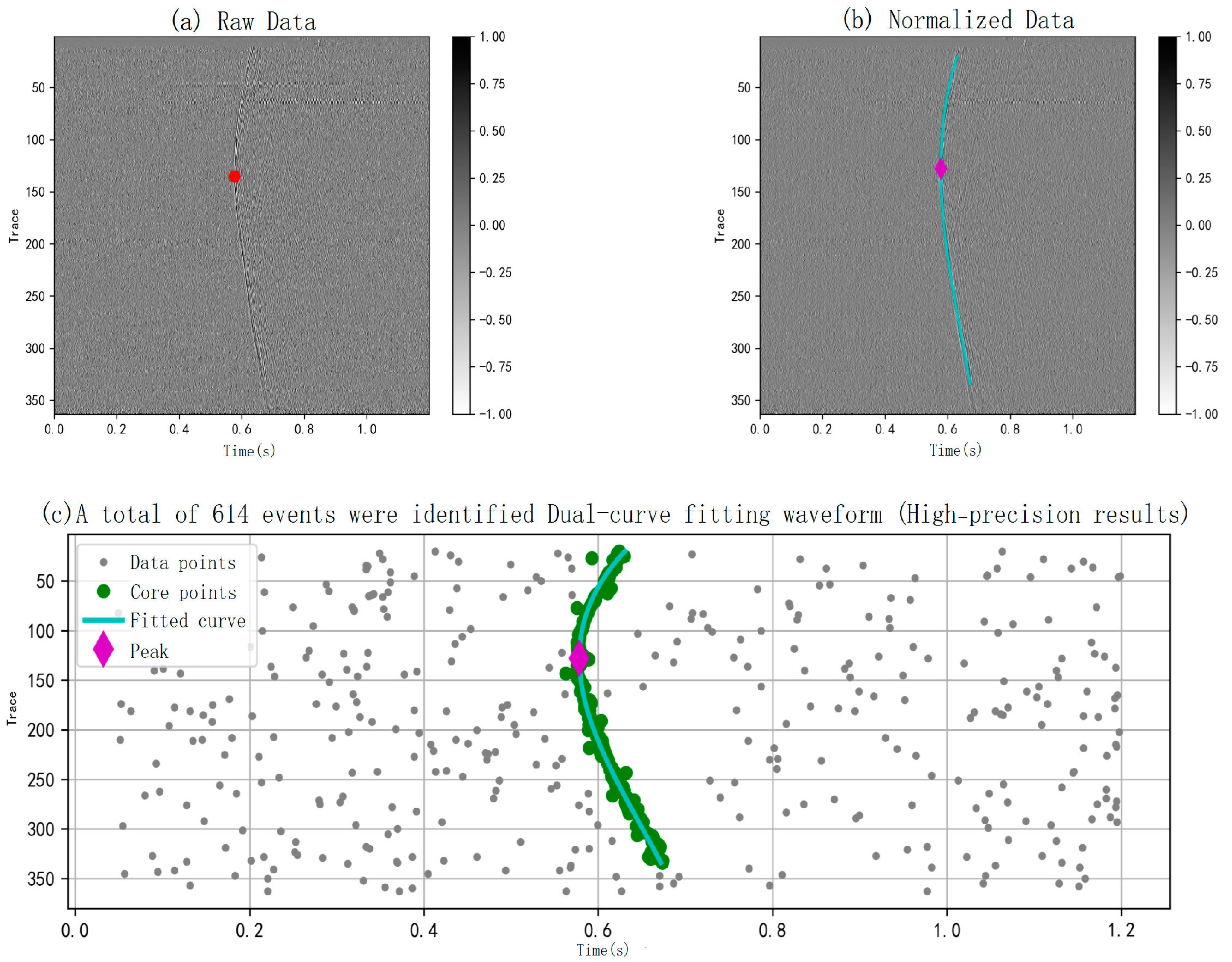
Processed waveform and hypocenter relocation for event 100001 from well XX.
Figure 7.
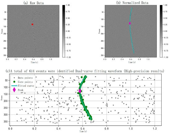
Processed waveform and hypocenter relocation for event 100014 from well XX.
In Figure 6 and Figure 7, the first arrival point of the microseismic wave in Figure 6a and Figure 7a is marked as a red dot (the point on the microseismic wave with an infinite slope is the first arrival point, which is the point where the processed data intersects the microseismic waveform through a straight line perpendicular to the x-axis). This point corresponds to the z-axis coordinate of the event point (the depth correction of the optical fiber is ignored in the vertical well). In Figure 6b,c and Figure 7b,c, the light blue lines correspond to the microseismic waveforms obtained by fitting the pick points, and the first arrival points of the microseismic wave picked by the machine are represented by purple diamond dots. Figure 6 and Figure 7 share the same organizational structure, both recording the results of automatic machine identification of an earthquake waveform. In Figure 6a,b and Figure 7a,b, each curve represents the time-domain record of a DAS channel within the event window. The waveform amplitude varies with the channel position, exhibiting abrupt amplitude changes at the channel cluster upon event arrival. Through waveform overlay and data processing, the entire waveform of the seismic wave is displayed in the heatmap. For comparative verification, the first arrival points were manually selected on the waveforms and compared with the points automatically identified by the machine. The error and accuracy of machine identification were examined through comparison with various events. The results are shown in Table 2, with most errors around 3%. Table 2 below verifies the accuracy of microseismic event detection by calculating the average values of the data from each event.
Table 2.
Accuracy verification of the automatic microseismic event identification algorithm.
Precision and recall were evaluated for Well XX. 2163 files from a specific well section were randomly selected for analysis (each file represents 1.2 s of DAS data). The algorithm identified 1177 files containing microseismic events. These 1177 microseismic event files (131 files were not detected by the algorithm but contained waveform clusters) and 986 unidentified files were then sampled and checked. Simultaneously, 290 identified files and 277 unidentified files were randomly selected for analysis at a 95% confidence level and a 5% error margin. Ultimately, 14 false positives were detected among the identified files, and 11 false positives were detected among the unidentified files. The calculated precision was 95.2%, and the false negative rate was 4.0%.
6. Conclusions and Recommendations
(1) A method for automatically picking and locating microseismic events based on dual-fit modeling and waveform inversion was designed and implemented. By using the DAS data from the actual well site to obtain the microseismic event cloud map for the corresponding period and placing all the generated microseismic sources in the three-dimensional wellbore profile, the degree of fracturing during hydraulic fracturing can be evaluated. A high number, wide distribution, and long extension of the source indicate that the fracture was well performed and that production may be improved in subsequent wells.
(2) After decomposing and reconstructing the original signal using the EMD method, all “event points” were obtained using the classic short-time average/long-time average energy ratio method. Seismic waveforms were obtained through DBSCAN density clustering and RANSAC robust fitting. Finally, the radial and vertical distances of the seismic source were obtained through mathematical modeling inversion, and the third component was approximated by fracture propagation information.
(3) Based on field experimental data from Well XX, and after comparison and judgment, this method can filter out approximately 80% of the high-frequency signals in the original data, achieving an automatic detection rate of 96% and an accuracy of 95%, with an actual error of approximately 3%.
(4) Due to the confidentiality of domestic well data, the testing scope in this paper is relatively small, lacking the ability to judge and detect multiple seismic waveforms at a fixed time step. Further improvements and verifications are needed. Meanwhile, existing methods still have room for improvement in the accuracy of seismic source location under complex geological conditions, and the data processing is relatively crude in order to facilitate engineering and enterprise use. More efficient and refined processing methods can be explored in future work.
(5) In the data processing of the article, the EMD method is not the optimal approach for processing DAS data. This method is only effective in suppressing high-frequency noise (above 200 Hz), but the processing of low-frequency noise (50 Hz to 200 Hz) and ultra-low-frequency noise (below 50 Hz) still requires further optimization. If the vibration of the pump unit and the interference from environmental vehicles in the actual well site are severe, the difficulty of extracting effective information will further increase. Another issue is that if the energy intensity of fluid noise and pipe waves in the pipeline is too high, effective information can hardly be extracted. Subsequent work will focus on conducting more detailed work on signal processing.
(6) In the overall algorithm, if this system is to be applied to real well sites, not only computational accuracy but also computational efficiency is required. The method in this paper can process 1 s of data in real time. If the filtering algorithm is iteratively upgraded or a more precise microseismic event-picking algorithm is used, a large amount of computing resources may be required. The estimated time for the original data after passing through the entire system will be several times or dozens of times longer than the original. Therefore, future researchers can conduct experiments by down-sampling DAS data or deleting unnecessary channels.
Author Contributions
Conceptualization, Z.Z.; methodology, Y.Y.; validation, Y.Y., Q.S. and K.S.; formal analysis, Y.Y.; investigation, Y.Y.; resources, K.S.; data curation, K.S.; writing—original draft preparation, Y.Y.; writing—review and editing, Y.Y.; visualization, Q.S.; supervision, Z.Z.; project administration, Z.Z. All authors have read and agreed to the published version of the manuscript.
Funding
This research received no external funding.
Institutional Review Board Statement
Not applicable.
Informed Consent Statement
Not applicable.
Data Availability Statement
The original contributions presented in this study are included in the article. Further inquiries can be directed to the corresponding author.
Acknowledgments
We would like to express our sincere gratitude to all the authors for their valuable contributions to this study. Special thanks go to Z.Z. for his insightful conceptualization of the research, as well as his rigorous supervision and efficient project administration throughout the process. We are indebted to Y.Y. for his dedicated efforts in developing the methodology, conducting formal analysis and investigation, performing validation, and drafting the original manuscript, along with careful review and editing to refine the paper. We also appreciate Q.S. for his contributions to validation work and clear scientific visualization, and K.S. for providing essential resources, undertaking meticulous data curation, and participating in the validation process. Finally, we thank all authors for their consensus on the final published version of this manuscript.
Conflicts of Interest
Author Kuan Sun was employed by the company Deep Earth Insights Data Technology Co., Ltd. The remaining authors declare that the research was conducted in the absence of any commercial or financial relationships that could be construed as a potential conflict of interest.
References
- Yang, C.X.; Yang, Z.Z.; Li, X.G.; Yi, L.P. Status and prospect of reservoir stimulation technologies for CBM surface well production in China. Nat. Gas Ind. 2022, 42, 154–162. [Google Scholar]
- Wang, Z.R.; Wen, Z.Y.; Chen, L.X. Productivity prediction of vertical test well for fractured coal reservoir under hydraulic fracturing. Nat. Gas Geosci. 2021, 32, 465–471. [Google Scholar]
- Dumitrache, L.; Roy, A.; Bird, A.; Goktas, B.; Sorgi, C.; Stanley, R.; De Gennaro, V.; Eswein, E. A Multidisciplinary Approach to Production Optimization through Hydraulic Fracturing Stimulation and Geomechanical Modelling in Clair Field. In Proceedings of the International Petroleum Technology Conference, Riyadh, Saudi Arabia, 21–23 February 2022. [Google Scholar]
- Li, Z.; Chang, X.; Yao, Z.X.; Wang, Y.B. Fracture monitoring and reservoir evaluation by microseismic method. Chin. J. Geophys. 2019, 62, 707–719. [Google Scholar]
- Hu, Z.F.; Kang, H.X.; Tian, Y.K.; Song, H.J.; Zhou, H.; Ma, Y.Y.; Wang, Y.F. Quantitative comparative analysis of monitoring effect of microseismic fracturing borehole and surface. Appl. Geophys. 2023, 20, 507–517+671–672. [Google Scholar]
- Zeng, R.; Lin, J.; Zhao, Y.J. Development situation of geophones and its application in seismic array observation. Prog. Geophys. 2014, 29, 2106–2112. [Google Scholar]
- Liang, B.Y.; Chang, L.; Fang, D.Z.; Gan, Y.; Zhang, J. Microseismic and its monitoring: Toward vector scanning of microseismic based on lower signal-to-noise ratio. Prog. Geophys. 2023, 38, 47–75. [Google Scholar]
- Da, S.J.; Li, X.G.; Dong, H.L.; Li, H.Y. Summary of Microseismic Location Methods. J. Jilin Univ. 2020, 50, 1228–1239. [Google Scholar]
- Chen, H. Horizontal well distributed fiber optic microseismic data processing and application. Fault-Block Oil Gas Field 2025, 32, 463–469. [Google Scholar]
- Hua, H.; Cheng, B.J.; Xu, T.J.; Zhenqian, Y.; Bo, G.; Cheng, H. Distributed optical fiber acoustic sensing-based optimization of microseismic source localization in the hydraulic fracturing for coalbed methane production. Coal Geol. Explor. 2025, 53, 191–204. [Google Scholar]
- Ding, X.P.; Wang, W.; Fu, L.C. Classification and Application Principles of Optical-Fibre Transducer. Spectrosc. Spectr. Anal. 2006, 26, 1176–1178. [Google Scholar]
- Huang, J.; Liang, Y.Z.; Zhong, X.X.; Jin, L.; Guan, B.O. Noise Analysis and Signal-to-Noise Ratio Enhancement of Fiber-Based Photoacoustic Microscopy. Chin. J. Lasers 2022, 49, 99–106. [Google Scholar]
- Wang, H.P. Influence of Interfacial Effect Between Distributed Optical Fiber Sensors and Monitored Structures. Acta Opt. Sin. 2022, 42, 32–42. [Google Scholar]
- Zhang, J.; Wu, Y.R.; Yang, H.B. Research on the design of optical fiber sensor considering the influence of vibration and temperature. Laser J. 2021, 42, 150–154. [Google Scholar]
- Diao, R.; Shan, L.Y.; Shang, X.M. The denoising method for microseismic monitoring data in time-frequency domain. Geophys. Geochem. Explor. 2015, 39, 112–117. [Google Scholar]
- Xing, Y.K.; Huang, B.X.; Chen, D.Y.; Xinglong, Z.; Binghong, L. Nonlinear Fracturing Characterization of Hydraulic Fracture: Utilizing Full-Waveform and Multi-Parameter Analysis Method of Acoustic Emission. J. China Coal Soc. 2021, 46, 3470–3487. [Google Scholar]
- Huang, N.E.; Shen, Z.; Long, S.R.; Wu, M.C.; Shih, H.H.; Zheng, Q.; Yen, N.C.; Tung, C.C.; Liu, H.H. The empirical mode decomposition and the Hilbert spectrum for non-linear and non-stationary time series analysis. Proc. R. Soc. Lond. A 1998, 454, 903–995. [Google Scholar] [CrossRef] [Scilit]
- Jia, R.S.; Zhao, T.B.; Sun, H.M.; Yan, X.H. Microseismic Signal Denoising Method Based on empirical mode decomposition and Independent Component Analysis. Chin. J. Geophys. 2015, 58, 1013–1023. [Google Scholar]
- Stevenson, R. Microearthquakes at Flathead Lake, Montana: A study using automatic earthquake processing. Bull. Seismol. Soc. Am. 1976, 66, 61–79. [Google Scholar]
- Wu, Z.T.; Li, S.X. Comparison of STA/LTA P-pickers for micro seismic monitoring. Prog. Geophys. 2010, 25, 1577–1582. [Google Scholar]
- Zhou, Y.W.; Liu, X.Q. A New Method of Automatic Seismic Event Detection. China Earthq. Eng. J. 2008, 2, 102–106+123. [Google Scholar]
- Ester, M.; Kriegel, H.; Sander, J.; Xu, X. A Density-Based Algorithm for Discovering Clusters in Large Spatial Databases with Noise. Knowl. Discov. Data Min. 1996, 96, 226–231. [Google Scholar]
- Feng, S.R.; Xiao, W.J. An Improved DBSCAN Clustering Algorithm. J. China Univ. Min. 2008, 37, 105–111. [Google Scholar]
- Luo, W.J.; Chu, F.D.; Heng, F.; Yang, X.; Feng, C. Research and application of DAS microseismic monitoring technology in shale gas exploration areas. In Proceedings of the China Petroleum Geophysical Exploration Conference, Urumqi, China, 10 December 2022. [Google Scholar] [CrossRef]

Disclaimer/Publisher’s Note: The statements, opinions and data contained in all publications are solely those of the individual author(s) and contributor(s) and not of MDPI and/or the editor(s). MDPI and/or the editor(s) disclaim responsibility for any injury to people or property resulting from any ideas, methods, instructions or products referred to in the content. |
© 2026 by the authors. Licensee MDPI, Basel, Switzerland. This article is an open access article distributed under the terms and conditions of the Creative Commons Attribution (CC BY) license.