Research on Frequency Modulated Continuous Wave (FMCW) Lidar Equation Based on Optical Mixing

Abstract

Frequency Modulated Continuous Wave (FMCW) lidar exhibits excellent anti-interference capabilities and efficient range and velocity measurement performance. Operating range is a crucial metric for FMCW lidar systems. To address the limitations of traditional radar equations, which do not account for optical mixing and balanced detection, a FMCW lidar equation based on optical mixing has been derived. This equation incorporates parameters such as the FMCW lidar system, average noise power, signal-to-noise ratio, and coherent detection gain, while also considering the relationship between atmospheric transmittance and operating range. Finally, an experimental FMCW lidar system with a wavelength of 1550 nm was constructed to test the operating range for water surface tar-gets. The experimentally measured average maximum range was 272.49 m, while the maximum operating range calculated using the derived lidar equation was 293.60 m, with a relative error of 7.74%, thereby validating the accuracy of the equation. This equation can be applied to evaluate the maximum operating range of FMCW lidar in various environments, such as autonomous driving and low-altitude surveillance, providing theoretical support for the design and performance assessment of FMCW lidar systems.

1. Introduction

Lidar is an active detection technology that utilizes lasers for imaging, reconnaissance, and ranging [1], featuring advantages such as high resolution, high precision, and strong anti-interference capability. Frequency-modulated continuous wave (FMCW) lidar represents the cutting edge of this technology [2,3], offering advantages such as a long operating range [4], high detection accuracy [5,6], and strong sensitivity [7], demonstrating good reliability in complex environments. Operating range is an important parameter for FMCW lidar, characterizing its detection capabilities. Correctly analyzing the maximum operating range of FMCW lidar is important in performance evaluation and design improvement.

The radar equation was first proposed by Norton and Omberg at the U.S. Naval Research Laboratory in their 1947 study, marking the beginning of theoretical radar performance analysis [8]. In 1980, Skolnik in Switzerland first proposed the theoretical model for frequency-modulated continuous waves but did not conduct in-depth discussions on rain–fog multiple scattering or speckle fading in frequency-modulated lasers [9]. In 1983, Shipley et al. [10] conducted the first systematic study of high-spectral-resolution lidar (HSRL) and explicitly provided mathematical relationships between lidar operating range and parameters such as echo power, scattering coefficient, and transmittance, addressing the deficiency of the lidar range equation, which lacks an atmospheric attenuation model. In 1999, Karlsson [11] first incorporated coherence length into the FMCW lidar equation and determined the optimal local oscillator (LO) power to evaluate the ultimate operating range limit. However, the coupling phenomenon between surface scattering and coherence attenuation was still not included in the model. In 2010, Chen Dong et al. [12] analyzed error sources in traditional lidar equations and proposed correction methods incorporating factors such as double scattering approximation, pulse waveform, and beam distribution. However, the corrected equation was computationally complex and did not consider target reflection or coherent detection scenarios. In 2012, Wang Tianqiao et al. [13] derived a radar equation suitable for focal plane laser imaging radar based on the traditional lidar equation. The Bidirectional Reflectance Distribution Function (BRDF) was used to replace the original radar cross-section in the derivation, but this equation did not consider laser beam characteristics. In 2016, Yang Hongzhi et al. [14] modified the lidar equation by introducing Gaussian beam transmission gain, fiber-receiving efficiency, and a Lambertian target scattering model, improving echo power calculation accuracy. However, aspects such as intermediate frequency bandwidth and LO noise were not addressed, lacking in-depth analysis of the signal-to-noise ratio model under coherent detection systems. In 2019, Siddiq et al. [15] systematically analyzed FMCW radar phase noise sources and propagation mechanisms, proposing a coherent mixing phase noise cancellation model that significantly improved operating range estimation accuracy and system signal-to-noise ratio prediction capabilities. However, joint modeling with parameters such as target radar cross-section and system losses was lacking. In the past five years, scholars such as Kyuho [16], Bima [17], and Lin Huizu [18] have optimized operating range models from perspectives such as processing gain, system losses, and target scattering characteristics; however, all lack discussion of coherent detection and optical mixing characteristics.

Addressing the aforementioned research deficiencies, this study focuses on the operating range of FMCW lidar and its influencing factors, establishing an FMCW lidar range equation. This equation considers the current FMCW lidar approach using couplers for optical mixing and balanced detectors for detection, introduces coherent detection gain and noise power, and analyzes the main noise sources of lidar and their effects. Finally, field experiments are conducted to verify the reliability of the optimized FMCW lidar range equation. This study provides a reference for subsequent research on optimizing relevant parameters and improving the performance of FMCW lidar systems.

2. FMCW Lidar Equation

Maximum operating range is a primary indicator for evaluating radar performance [19], and the maximum operating range of radar can be determined using the radar range equation. Since lasers and microwaves used in conventional radar are both electromagnetic waves, the lidar equation can be derived following the microwave radar equation derivation approach.

2.1. Derivation of Lidar Equation

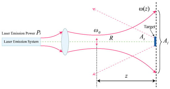
The laser emission process is shown in Figure 1. The emitted laser is typically a Gaussian beam; its cross-sectional amplitude distribution conforms to a Gaussian function, and the spot size varies according to a hyperbolic law along the light propagation direction [14]. ${\omega }_0$ represents the beam waist radius, $\omega (z)$ represents the laser spot radius at the target, $A_l$ represents the laser spot area at the target, and $A_t$ represents the effective reflective area of the target.

Figure 1. Laser emission process.

Assume that the power $P_r$ received by the radar depends on the transmitted power $P_t$, propagation distance R, and the target’s reflection characteristics [20]. In the radiation direction with radar transmitted antenna gain, $G_t$, the power density of the radar signal transmitted through the antenna after traveling distance R is

$$S_1={\displaystyle \frac{P_t{G}_t}{4\pi R^2}}$$

(1)

The unit of power density is ${\mathrm{W}/\mathrm{m}}^2$.

According to Figure 1, assuming the solid angle subtended by the emitted laser from the radar to the target position is ${\Omega }_t$, then ${\Omega }_t={\displaystyle \frac{{\omega }^2(z)}{R^2}}$ [14]. At this point, the lidar transmission gain is

$$G_t={\displaystyle \frac{4\pi }{{\Omega }_t}}$$

(2)

Considering the atmospheric transmittance, ${\tau }_{\alpha }$, and the transmit optical system transmittance ${\tau }_t$ of the lidar, combining Equations (1) and (2), the target irradiance (power density of the laser at the target position) is

$$E_{\mathrm{in}}={\displaystyle \frac{P_t{\tau }_{\alpha }{\tau }_t}{{\Omega }_t{R}^2}}$$

(3)

After the target is illuminated, it produces a diffuse reflection. The target’s scattering power is related to the target’s reflection characteristics. In microwave radar, the radar cross-section (RCS) $\sigma$ is commonly used to characterize target reflection characteristics. In lidar, the emitted laser satisfies geometric optical properties and can be described using the Bidirectional Reflectance Distribution Function (BRDF). BRDF is defined as [21,22]

$$f_t({\theta }_i,{\varphi }_i,{\theta }_r,{\varphi }_r)={\displaystyle \frac{d{L}_{\mathrm{out}}({\theta }_i,{\varphi }_i,{\theta }_r,{\varphi }_r)}{d{E}_{\mathrm{in}}({\theta }_i,{\varphi }_i)}}$$

(4)

In the above equation, $L_{\mathrm{out}}$ is the outgoing luminance; ${\theta }_i$ and ${\varphi }_i$, as well as ${\theta }_r$ and ${\varphi }_r$, are the azimuth and elevation angles of the incident and outgoing directions, respectively. For a Lambertian surface, the BRDF expression can be simplified to

$$f_t^{\mathrm{Lambertian}}({\theta }_i,{\varphi }_i,{\theta }_r,{\varphi }_r)={\displaystyle \frac{{\rho }_t}{\pi }}$$

(5)

In the above equation, ${\rho }_t$ is the target reflectivity.

Assuming the effective receiving area of the lidar is $A_r$, and the transmittance of the receiving optical system is ${\tau }_r$, the laser power received by the lidar is

$$P_R=L_{\mathrm{out}}{\tau }_{\alpha }{\tau }_r\cdot {\displaystyle \frac{A_r}{R^2}}\cdot A_t={\displaystyle \frac{P_t{\tau }_{\alpha }^2{\tau }_t{\tau }_r{A}_t{A}_r{\rho }_t}{\pi {\Omega }_t{R}^4}}$$

(6)

The above is the lidar equation.

If the target is an extended target, where the laser spot is completely projected onto the target, then $A_t=A_l={\Omega }_t{R}^2$; substituting into Equation (6), the lidar equation for extended targets can be calculated as

$$P_R={\displaystyle \frac{P_t{\tau }_{\alpha }^2{\tau }_t{\tau }_r{A}_r{\rho }_t}{\pi R^2}}$$

(7)

Equation (7) shows that for extended targets, the received laser power is proportional to the square of the distance.

2.2. Derivation of FMCW Lidar Equation

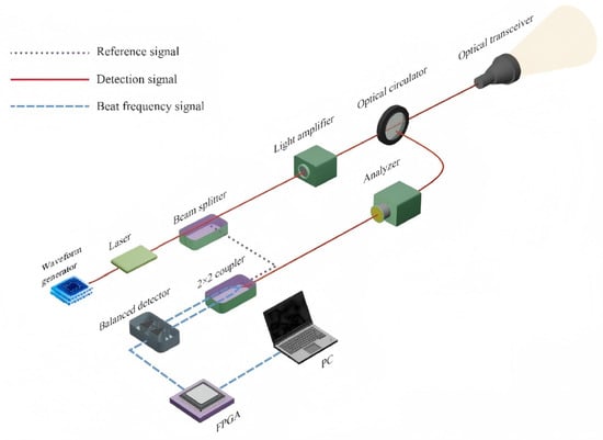
Figure 2 shows the basic ranging principle diagram of the FMCW lidar. FMCW lidar uses modulated continuous laser signals to measure target distance and velocity by obtaining an intermediate frequency signal through interference between the transmitted and received light. The system employs a linear frequency-modulated chirped laser as both the transmit signal and LO signal, mixing the target echo signal with the LO signal at the photodetector. The intermediate frequency signal obtained through mixing can demodulate the target’s distance information. Due to the use of coherent detection, FMCW lidar can directly measure the velocity of moving objects by sensing the Doppler frequency shift of light.

Figure 2. FMCW lidar ranging principle diagram.

Since the system utilizes optical mixing, a balanced photodetector (BPD) is employed for detection to suppress the direct current (DC) component.

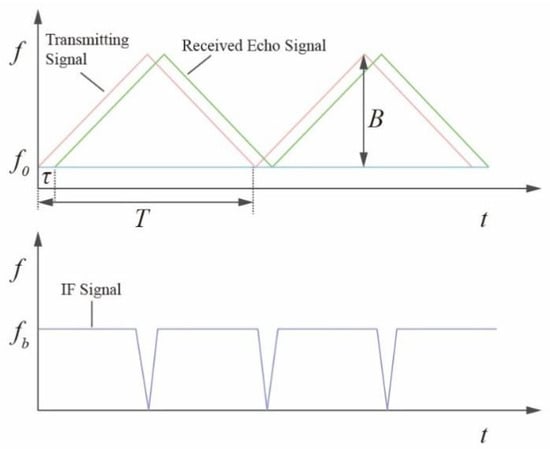
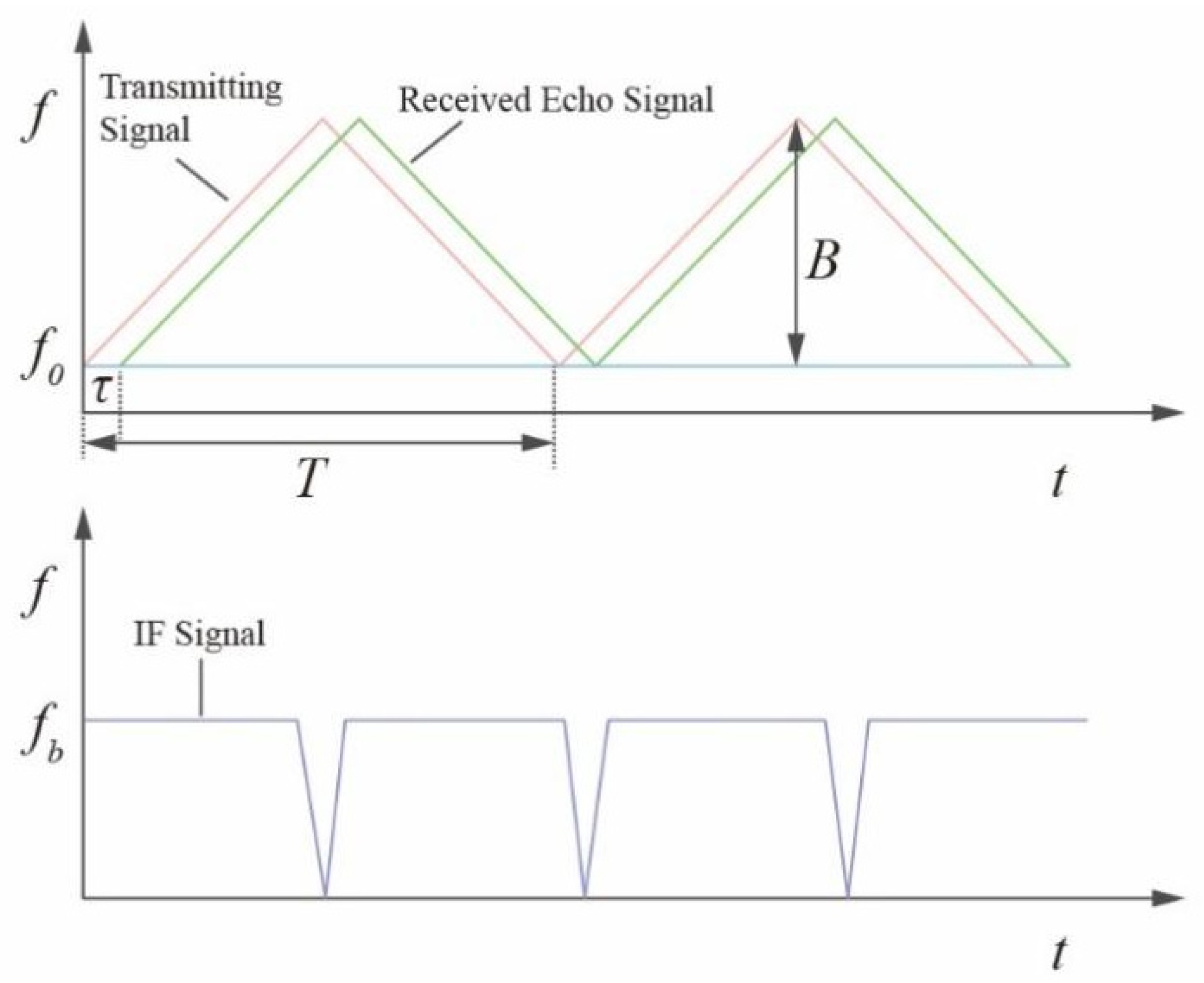
The frequency modulation curves of the transmitted and echo signals in FMCW radar are shown in Figure 3.

Figure 3. Triangular wave signal frequency modulation curve.

In the figure above, $f_0$ is the initial frequency of the frequency-modulated signal, $\tau$ is the echo signal time delay, $k=B/T$ is the frequency sweep slope, B is the sweep bandwidth, and T is the sweep period.

Let ${\omega }_{1-\tau }=2\pi f_0+\pi k(t-\tau )$ be the angular frequency of the echo light, and ${\omega }_t=2\pi f_0+\pi kt$ denote the angular frequency of the LO light. The optical electric fields corresponding to the echo light and LO light are, respectively,

$$\begin{array}{l}{E}_R(t)=E_R\cos \left[{\omega }_{t-\tau }(t-\tau )+{\phi }_R\right]\\ E_{LO}(t)=E_{LO}\cos \left({\omega }_{t}t+{\phi }_{LO}\right)\end{array}$$

(8)

To simplify the calculation, the above equation is written in complex form. Since coherent detection extracts the frequency difference between two input beams (i.e., the instantaneous frequency of the intermediate frequency signal), $E_{LO}(t)$ needs to be rewritten in conjugate form [23,24].

$$\begin{array}{l}{E}_R(t)=E_R{e}^{i\left[{\omega }_{i-\tau }(t-\tau )+{\phi }_R\right]}\\ E_{LO}^{*}(t)=E_{LO}{e}^{-i\left({\omega }_{i}t+{\phi }_{LO}\right)}\end{array}$$

(9)

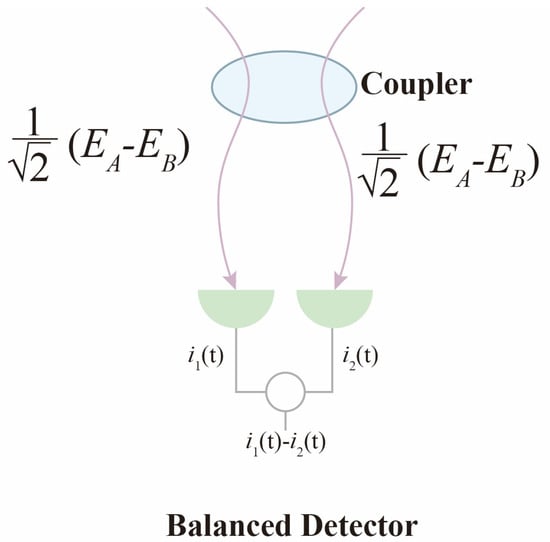
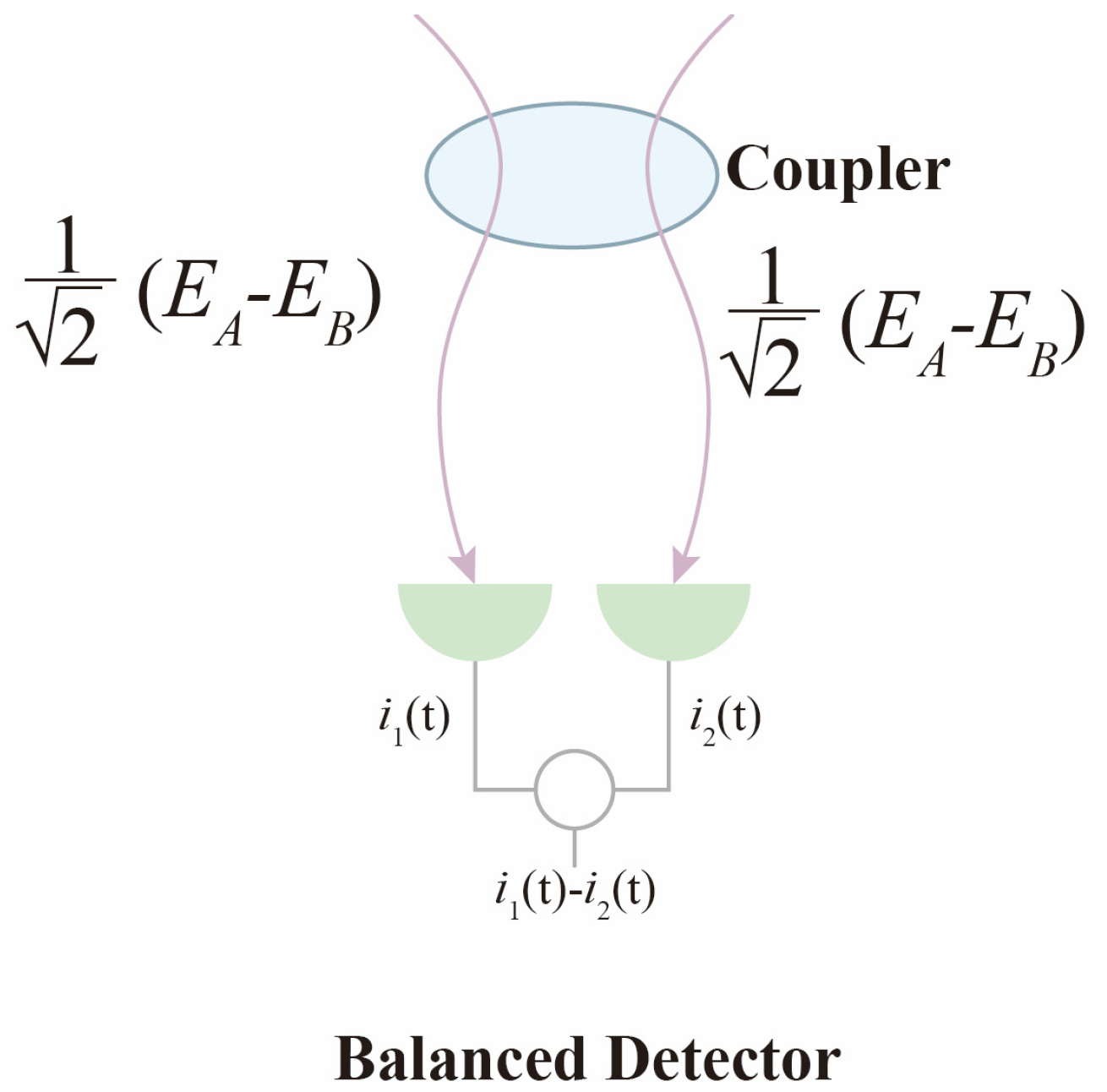
The principle of the balanced photodetector is shown in Figure 4.

Figure 4. Balanced photodetector principle.

The LO light and echo light interfere at the coupler, and after interference, the light is split equally into two paths, outputting to the balanced detector. Since the light is split into two paths, the optical power corresponding to each path is $1/2$ of the original optical power. Furthermore, because optical power is proportional to the square of the optical electric field intensity, the optical electric field intensity corresponding to each path is $1/\sqrt{2}$ of the original optical electric field intensity.

The optical electric field intensity $E_1(t)$ of the first path is

$$\begin{array}{l}{E}_1(t)={\displaystyle \frac{1}{\sqrt{2}}}[E_R(t)+E_{LO}^{*}(t)]\\ \hspace{1em} ={\displaystyle \frac{1}{\sqrt{2}}}{E}_R{e}^{i\left[{\omega }_{1-\mathrm{r}}(t-\tau )+{\phi }_R\right]}+{\displaystyle \frac{1}{\sqrt{2}}}{E}_{LO}{e}^{-i\left({\omega }_{i}t+{\phi }_{LO}\right)}\end{array}$$

(10)

Then, the corresponding photocurrent is

$$\begin{array}{l}{i}_1(t)=\mathrm{R}{[E_1(t)]}^2\\ \hspace{1em}\hspace{1em}={\displaystyle \frac{1}{2}}\left\{E_R^2{e}^{2i[{\omega }_{t-\tau }(t-\tau )+{\phi }_R]}+E_{LO}^2{e}^{2i({\omega }_{t}t+{\phi }_{LO})}+2E_R{E}_{LO}{e}^{i[{\omega }_{t-\tau }(t-\tau )-{\omega }_{t}t+{\phi }_R-{\phi }_{LO}]}\right\}\end{array}$$

(11)

In the above equation, $\mathrm{R}$ represents the responsivity of one path in the balanced photodetector.

The optical electric field intensity of the second $E_2(t)$ path is

$$\begin{array}{l}{E}_2(t)={\displaystyle \frac{1}{\sqrt{2}}}[E_R(t)-E_{LO}^{*}(t)]\\ \hspace{1em}\hspace{1em}={\displaystyle \frac{1}{\sqrt{2}}}{E}_R{e}^{i\left[{\omega }_{1-\mathrm{r}}(t-\tau )+{\varphi }_R\right]}-{\displaystyle \frac{1}{\sqrt{2}}}{E}_{LO}{e}^{-i\left({\omega }_{i}t+{\phi }_{LO}\right)}\end{array}$$

(12)

Then, the corresponding photocurrent is

$$\begin{array}{l}{i}_2(t)=\mathrm{R}{[E_2(t)]}^2\\ \hspace{1em}\hspace{1em}={\displaystyle \frac{1}{2}}\left\{E_R^2{e}^{2i[{\omega }_{t-\tau }(t-\tau )+{\phi }_R]}+E_{LO}^2{e}^{2i({\omega }_{t}t+{\phi }_{LO})}-2E_R{E}_{LO}{e}^{i[{\omega }_{t-\tau }(t-\tau )-{\omega }_{t}t+{\phi }_R-{\phi }_{LO}]}\right\}\end{array}$$

(13)

The output current of the balanced photodetector $i(t)$ is the difference between $i_1(t)$ and $i_2(t)$:

$$i(t)=i_1(t)-i_2(t)=2\mathrm{R}{E}_R{E}_{LO}{e}^{i[{\omega }_{t-\tau }(t-\tau )-{\omega }_{t}t+{\phi }_R-{\phi }_{LO}]}$$

(14)

Let $\phi ={\phi }_R-{\phi }_{LO}$; since the echo light power and the LO power are $P_R={\displaystyle \frac{E_R^2}{2}}$, the above equation can be rewritten as $P_{LO}={\displaystyle \frac{E_{LO}^2}{2}}$:

$$i(t)=4\mathrm{R}\sqrt{P_R{P}_{LO}}{e}^{i[{\omega }_{t-\tau }(t-\tau )-{\omega }_{t}t+\phi ]}$$

(15)

For direct detection lidar, the photocurrent $i^{\prime }(t)$ is

$$\begin{array}{l}{i}^{\prime }(t)=\mathrm{R}{[E_R(t)]}^2\\ ={\displaystyle \frac{1}{2}}\mathrm{R}{E}_R^2\{1+\cos [2{\omega }_{t-\tau }(t-\tau )+2{\phi }_R]\}\\ =\mathrm{R}{P}_R\{1+\cos [2{\omega }_{t-\tau }(t-\tau )+2{\phi }_R]\}\end{array}$$

(16)

Comparing Equations (15) and (16), it can be seen that under the same echo power, the gain G of coherent detection relative to direct detection is

$$G={\displaystyle \frac{4\mathrm{R}\sqrt{P_R{P}_{LO}}}{\mathrm{R}{P}_R}}=4\sqrt{{\displaystyle \frac{P_{LO}}{P_R}}}$$

(17)

Rewriting Equation (7) with the operating range on the left side of the equation yields

$$R^2={\displaystyle \frac{P_t{\tau }_{\alpha }^2{\tau }_t{\tau }_r{A}_r{\rho }_t}{\pi P_R}}$$

(18)

Let the FMCW lidar signal-to-noise ratio (SNR) be $R_{SN}$; then, $R_{SN}=P_R/P_N$, where $P_N$ is the noise power.

In summary, by introducing the coherent detection gain G and lidar signal-to-noise ratio $R_{SN}$ into Equation (18), the FMCW lidar operating range equation for extended targets can be obtained as

$$R^2={\displaystyle \frac{P_t{\tau }_{\alpha }^2{\tau }_t{\tau }_r{A}_r{\rho }_{t}G}{\pi R_{SN}{P}_N}}$$

(19)

3. FMCW Lidar Equation Parameter Analysis

Analyzing Equation (19), the parameters ($P_t$, ${\tau }_t$, ${\tau }_r$, etc.) are determined values, while quantities such as noise power $P_N$, atmospheric transmittance ${\tau }_{\alpha }$, and coherent detection gain G are more complex and require further analysis.

3.1. FMCW Lidar Noise Power

FMCW lidar noise power determines the magnitude of the signal-to-noise ratio. The smaller the noise power, the higher the signal-to-noise ratio and the better the performance when the received echo power remains constant. Noise power is typically calculated using the following equation [25]:

$$P_N=\sqrt{P_q\cdot \left(P_{Rec}+P_B\right)+NE{P}^2\cdot \Delta f_D}$$

(20)

In the above equation, $P_q$ is the equivalent quantum noise power, $P_B$ is the background power, $P_{Rec}$ is the AC optical signal amplitude, NEP is the noise equivalent power, and $\Delta f_D$ is the detector electrical bandwidth. Equation (20) is divided into two terms because quantum noise depends on incident optical power and must be described separately with a term related to optical power. The noise corresponding to NEP is the detector’s intrinsic noise, which is independent of optical power. In approximate calculations, the noise current that directly calculates shot noise can be substituted into the expression for noise equivalent power NEP, where $P_N=\sqrt{NE{P}^2\cdot \Delta f_D}$.

The expression for noise equivalent power, NEP, is shown in Equation (21):

$$NEP={\displaystyle \frac{I_N}{\mathrm{R}\cdot \sqrt{\Delta f_D}}}$$

(21)

In the above equation, $I_N$ is the detector’s total noise current.

According to noise sources, lidar noise can be classified into four categories: laser noise $I_L$, detector noise $I_S$, environmental noise $I_B$, and digital processing noise $I_{DSP}$. The $I_N$ calculation method is

$$I_N=\sqrt{I_L^2+I_S^2+I_B^2+I_{DSP}^2}$$

(22)

By analyzing various noise currents, the value of NEP can be calculated, then the noise power P_N can be calculated.

3.1.1. Laser Noise

During the laser generation process, spontaneous emission phenomena inevitably occur, causing disordered disturbances in the optical wave phase and amplitude, manifesting as spectral linewidth broadening and unstable fluctuations in output optical power. Among these, random intensity disturbances are called intensity noise, random frequency disturbances are called frequency noise, and random phase disturbances are called phase noise. The intensity noise of single-frequency fiber lasers is mainly affected by technical noise in the low-frequency range and relaxation oscillation noise in the mid-frequency range.

Frequency noise manifests as deviation from frequency modulation linearity in FMCW systems; phase noise is the time-domain integral representation of frequency noise. When the lidar performs short-range ranging, the phase noise is partially offset during the frequency mixing process, and detector noise becomes the dominant factor. For long-range detection, the increased time delay of the echo signal weakens the correlation between the phase noise of the transmitted signal and the echo, resulting in a diminished cancellation effect in coherent reception and a gradual increase in phase noise [26,27]. The lidar selected in this paper has a maximum laser linewidth of 200 kHz and a coherence length greater than 1500 m, which is significantly higher than the effective operating range of the lidar.

Intensity noise mainly originates from factors such as pump source noise and temperature fluctuations. In a balanced detector, the intensity noise received by the two photodiodes is in-phase, and they cancel each other out; thus, it does not appear in the output intermediate frequency signal.

3.1.2. Detector Noise

The noise performance of the balanced photodetector directly determines the system’s sensitivity limit. Detector noise mainly includes shot noise, dark current noise, and thermal noise [28]. These noises are all random processes and are among the most significant noise sources in the signal.

Shot noise originates from the randomness of photoelectron emission and is an inherent quantum noise in the photon detection process. Under strong LO light settings, shot noise plays a dominant role. The mean square current of shot noise is

$${\sigma }_{LO}=\sqrt{2e\cdot I_{LO}\cdot \Delta f_D}$$

(23)

In the above equation, e is the electron charge, with a magnitude of 1.602176634 × 10⁻¹⁹ C, and $I_{LO}$ is the LO current.

Dark current noise is the noise generated by leakage current that still exists in the detector under no-light conditions. Its characteristics are similar to shot noise but originate from thermally excited carriers. The mean square current of dark current noise is

$${\sigma }_{dark}=\sqrt{2\cdot e\cdot I_{dark}\cdot \Delta f_D}$$

(24)

In this context, $I_{dark}$ represents the dark current. For high-performance InGaAs-balanced photodetectors, dark current noise minimally impacts system performance.

Thermal noise (Johnson–Nyquist noise) originates from the thermal motion of resistors in the detector and preamplifier and follows a Gaussian distribution, and its intensity is proportional to temperature and bandwidth. The mean square current of thermal noise is

$${\sigma }_{\mathrm{th}}=\sqrt{{\displaystyle \frac{4kTB}{R_L}}}$$

(25)

where k is Boltzmann’s constant, with a magnitude of $1.38\times {10}^{-23}$ J/K, T is the absolute temperature, and $R_L$ is the load impedance.

3.1.3. Digital Processing Noise

The noise in the digital processing chain mainly comes from ADC quantization noise and clock jitter. These noises affect the precision of digital signal processing, especially the peak detection results after Fast Fourier Transform (FFT).

Digital processing noise has a minimal impact on FMCW lidar. The ranging information in FMCW is carried in narrowband single-frequency difference frequency signals, whose frequency-domain energy is concentrated with clear characteristics. By contrast, digital processing noises, such as ADC quantization and amplifier noise, are mostly wideband random signals, which can be clearly separated in the frequency domain. FMCW ranging accuracy depends on frequency rather than amplitude, so digital noise minimally interferes with core parameters.

3.1.4. Environmental Noise

Environmental noise mainly includes background light interference, multipath reflection, and atmospheric scattering. These noises reduce the system’s signal-to-noise ratio and increase the false alarm rate.

Since FMCW lidar systems employ coherent detection and difference frequency signal extraction technology, they have a significant ability to suppress environmental noise. FMCW systems transmit continuous laser signals with linearly chirped frequency; mix the target-reflected echo signal with the local reference signal to generate a difference frequency signal proportional to the target distance; and ultimately, achieve ranging through spectral analysis. Environmental noise mostly comprises non-coherent wideband signals with randomly fluctuating phase and amplitude, unable to form stable coherent beat frequencies with the local reference signal. After mixing, environmental noise only transforms into random background noise, which can be filtered out by algorithms such as Fourier transform.

Based on the above analysis, under conditions of relatively high LO optical power, shot noise plays a dominant role in FMCW lidar. In engineering practice, shot noise is typically treated directly as Additive White Gaussian Noise (AWGN).

3.2. Atmospheric Transmittance ${\tau }_{\alpha }$

This study uses MODTRAN (PcModWin5 v1.3.3 Release Version) to simulate atmospheric transmittance ${\tau }_{\alpha }$. This software employs “three-dimensional radiative transfer paths” that are segmental, vertically variable, and tiltable to replace “distance.” It calculates the altitude and distance evolution of pressure, temperature, humidity, aerosols, and molecular absorption cross-sections in real-time at every meter, thereby providing transmittance curves that accurately correspond to path length, path geometry, and atmospheric non-uniform distribution. MODTRAN naturally applies to arbitrary long-distance, non-horizontal, and non-uniform atmospheric scenarios through layer-by-layer radiative transfer equation solving, with accurate calculations. By fitting the atmospheric transmittance results calculated by MODTRAN at different distances, we can obtain a fitting function of atmospheric transmittance versus operating range.

According to the Lambert–Beer law, when a collimated beam propagates in a uniform atmosphere, the transmittance satisfies the equation ${\tau }_{\alpha }=e^{-\alpha R}$, where $\alpha$ is the atmospheric extinction coefficient. This exponential form is the only analytical solution to the radiative transfer equation under single extinction and path uniformity conditions, and it is the default function describing atmospheric transmittance variation with distance. Therefore, we selected the exponential function as the fitting function for variation in atmospheric transmittance with distance.

3.3. Signal-to-Noise Ratio (SNR)

The SNR of an FMCW lidar is defined as the ratio of the received signal power to the total noise power. It serves as a key metric for evaluating the system’s detection capability, directly determining the target detection probability, false alarm probability, and upper limit of the operating range. Reference [11] provides an expression for the SNR of an FMCW lidar:

$$R_{SN}={\displaystyle \frac{{\eta }_{tot}(R)P_R(R)\exp \left(-\frac{2R}{c{\tau }_c}\right)}{h\nu B+\frac{{\eta }_{tot}(R)}{{\eta }_{lin}}\cdot \frac{P_R(R){\tau }_c}{\pi }\left[1-\exp \left(-\frac{2R}{c{\tau }_c}\right)\left(1+\frac{2R}{c{\tau }_c}\right)\right]B}}$$

(26)

In the above equation, ${\eta }_{tot}$ represents the overall efficiency of the FMCW lidar, $P_R(R)$ denotes the laser received power, $h\nu$ refers to the energy of a single photon, $B$ is the detection bandwidth, ${\eta }_{lin}$ stands for the linear efficiency, and ${\tau }_c$ represents the laser coherence time. This formula takes into account factors such as limitations associated with the temporal and frequency stability of the frequency-modulated emission of the lidar, as well as coupling efficiency. The impact of these factors on the actual SNR is reflected in the overall efficiency ${\eta }_{tot}$. Calculating the SNR of an FMCW lidar using this formula is quite complex. When evaluating the maximum operating range of an FMCW lidar, we are more concerned with the threshold SNR, denoted as $R_{SN}^{\prime }$. $R_{SN}^{\prime }$ is a parameter set by the lidar signal processing system. Signals exceeding this threshold value will be processed and displayed as point clouds, while signals below this threshold will be filtered out as noise.

3.4. Coherent Detection Gain

Equation (17) provides the expression for gain G. Substituting the expression for echo light power $P_R$ yields

$$G=4\sqrt{{\displaystyle \frac{P_{LO}}{P_R}}}=4\sqrt{{\displaystyle \frac{\pi P_{LO}}{P_t{\tau }_t{\tau }_r{A}_r{\rho }_t}}}\cdot {\displaystyle \frac{R}{{\tau }_{\alpha }}}$$

(27)

As shown in Section 3.2, the atmospheric transmittance ${\tau }_{\alpha }$ is only a function of the operating range R. All other values in the equation can be regarded as constants, so the expression for G is only related to R. Substituting Equation (27) into Equation (19), the operating range equation is

$$R={\displaystyle \frac{4{\tau }_{\alpha }\sqrt{P_{LO}{P}_t{\tau }_t{\tau }_r{A}_r{\rho }_t}}{\sqrt{\pi }{R}_{SN}{P}_N}}$$

(28)

In summary, by analyzing FMCW lidar noise power $P_N$, atmospheric transmittance ${\tau }_{\alpha }$, and coherent detection gain G, and substituting into Equation (28), we can obtain an implicit function equation of operating range containing only R. Using iterative calculation, the lidar operating range R can be accurately calculated.

4. Operating Range Model Example Calculation

4.1. FMCW Lidar Parameters

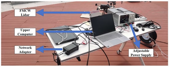
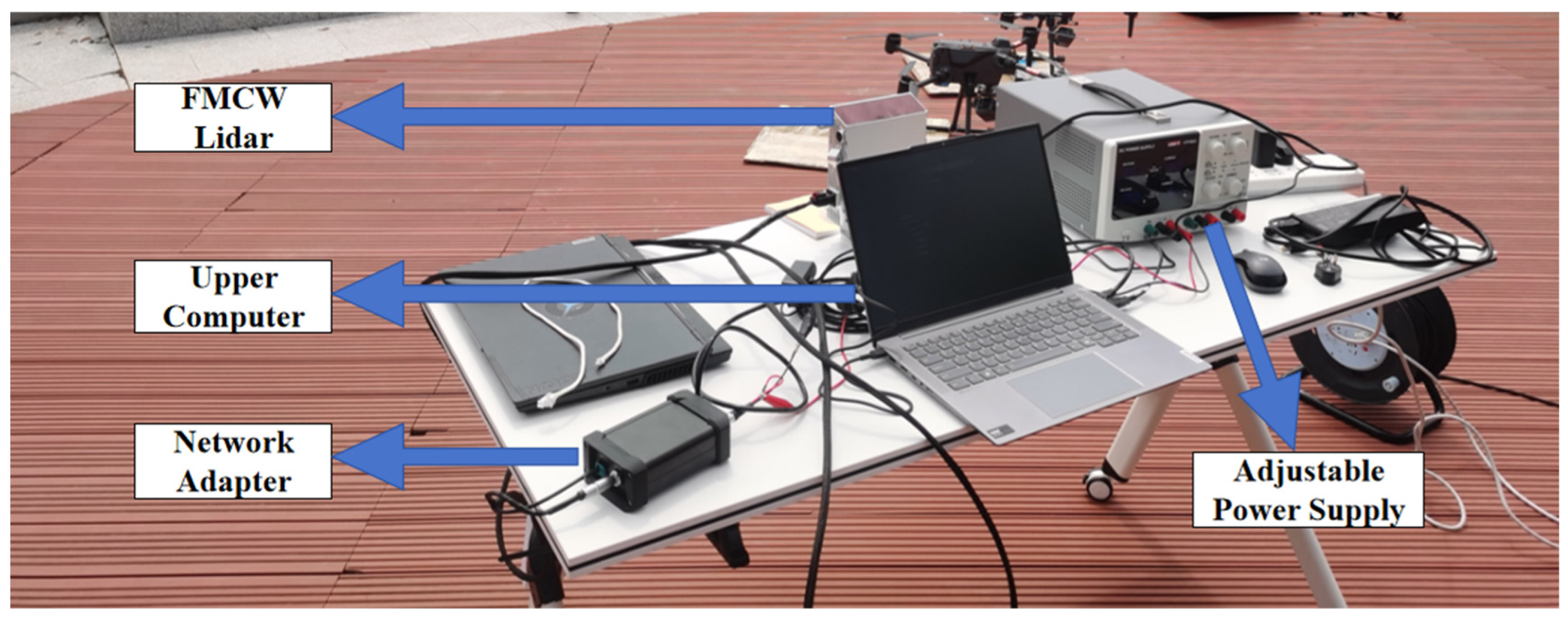
A specific FMCW lidar system is used for experimental verification. The FMCW lidar hardware system includes an integrated lidar, a network adapter, an adjustable power supply, and a host computer, as shown in Figure 5.

Figure 5. FMCW lidar experimental system.

The laser module is the emission source for laser signals, using a 1550 nm wavelength (eye-safe level) with linear frequency modulation support. The bandwidth is adjustable within the 2/4/6/10 GHz range, and when coupled with an amplifier to boost transmission power, it ensures long-range detection capability. The scanning system consists of two parts: a rotating mirror scanning subsystem and a galvanometer scanning subsystem. The rotating mirror scanning subsystem is composed of a rotating mirror motor and a five-facet mirror; it is responsible for horizontal scanning, achieving 120° horizontal field of view coverage through mirror rotation, with each mirror facet having an effective working range of 120° (24° redundancy for stray light suppression). The galvanometer scanning subsystem is composed of a galvanometer motor, a drive circuit, and a galvanometer mirror; it is responsible for vertical scanning, achieving 25° vertical field of view coverage through galvanometer angle adjustment, totaling 120 lines with a minimum vertical resolution of 0.08°. The laser transmits through an optical module with a divergence angle of 0.56 mrad horizontally and 0.14 mrad vertically. After the light source returns, it is received through the optical module, undergoes optical mixing internally, and uses a balanced photodetector as the receiving device with a processing bandwidth greater than 300 MHz. It efficiently receives and converts returned optical signals into electrical signals, providing a foundation for subsequent signal processing.

The adjustable power supply uses the UNI-T UTP3603, which employs linear power supply technology to provide pure and stable DC output.

One end of the network adapter box is connected to the lidar via power and network cables, while the other end’s power cable connects to the adjustable power supply, and the network cable connects to the host computer, serving both power adaptation and network adaptation functions.

The host computer can store the original signals received by the lidar photodetector and the angular information from the scanning system, facilitating subsequent signal processing. The main parameters of this lidar are shown in Table 1.

Table 1. Parameters of FMCW lidar.

Parameter	Value
$P_{\mathrm{t}}$	100 mW
${\tau }_{\mathrm{t}}$	0.7
${\tau }_{\mathrm{r}}$	0.7
$\mathrm{R}$	0.95 A/W
D	3.2 cm
$P_{LO}$	1 mW
$\Delta f_D$	1.5 GHz
NEP (BPD)	9 $\mathrm{pW}/\sqrt{\mathrm{Hz}}$

In the table, D is the clear aperture of the receiving optical system, so the effective receiving area $A_{\mathrm{r}}$ is

$$A_{\mathrm{r}}=\pi {\left({\displaystyle \frac{D}{2}}\right)}^2\approx 8.0425\times {10}^{-4}{\mathrm{m}}^2$$

(29)

4.2. Field Experiment Verification

4.2.1. Field Experimental Environment

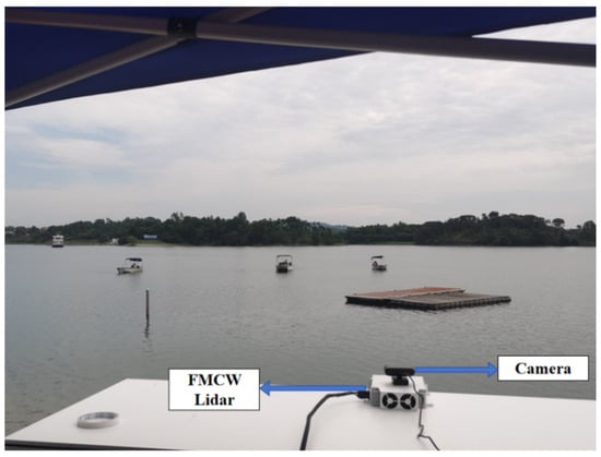
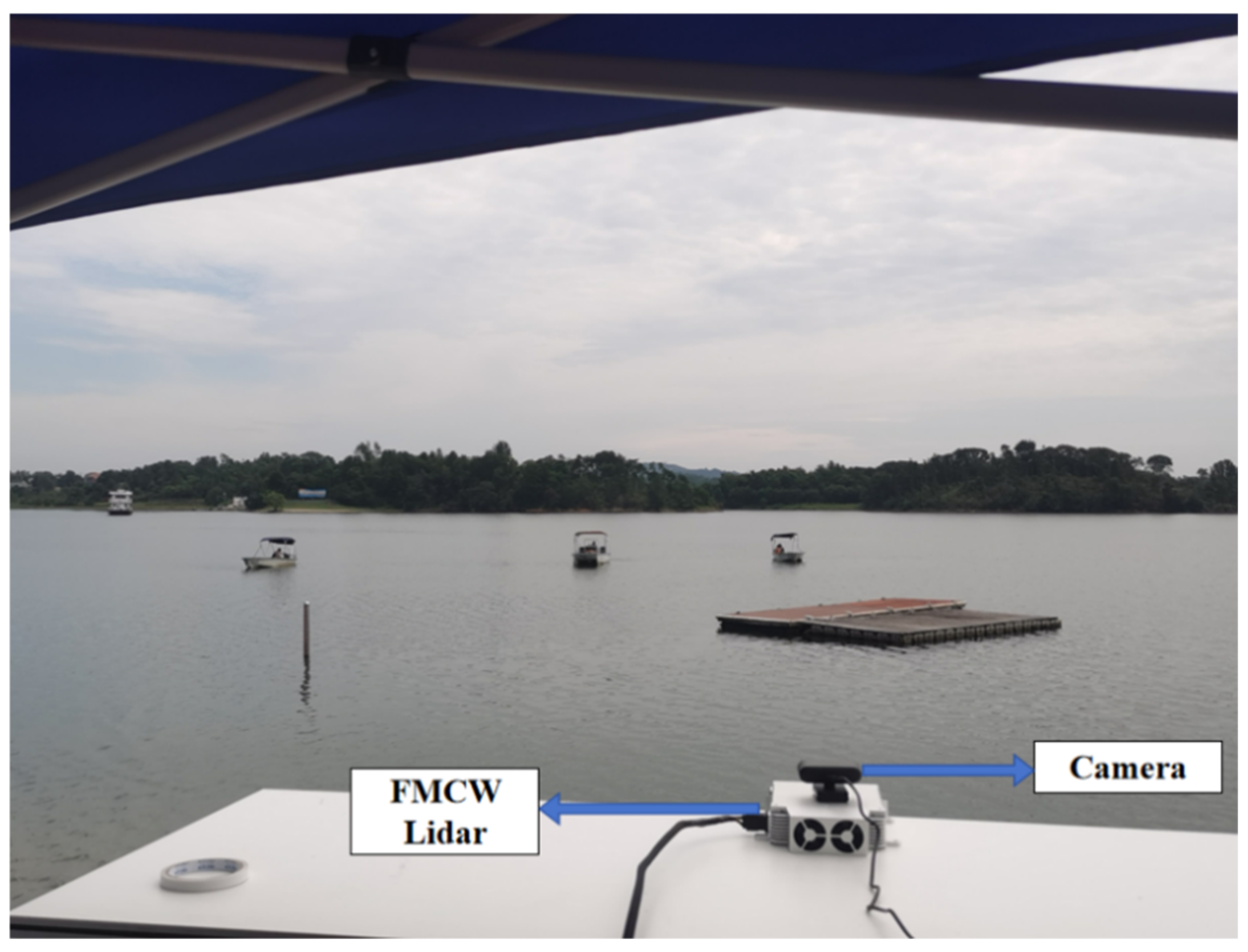
To verify the optimized FMCW lidar operating range model presented in this study, we designed a dynamic target test scenario. The experiment was conducted at 10:25 A.M. on 26 August 2025. The weather was cloudy with an on-site temperature of 34 °C. The location was a lake surface in Huangpi District, Wuhan City, for field experiments, with three jet skis as test targets. The hull of the jet skis is made of glass-fibre-reinforced plastic (GFRP), and its outer layer is coated with white gel coat (TiO₂—Polyester resin lacquer). The overall reflectivity of this coating for infrared light with a wavelength of 1550 nm has been measured to be 0.75. The experimental site environment is shown in Figure 6.

Figure 6. Experimental site environment.

MODTRAN was used to calculate atmospheric transmittance ${\tau }_{\alpha }$ at a 1550 nm wavelength for different distances. The MODTRAN parameter settings are shown in Table 2.

Table 2. MODTRAN parameter settings.

Input Parameter	Value
Calculation option	MODTRAN
Model atmosphere	Mid-latitude summer
Type of atmospheric path	Horizontal path
Mode of execution	Transmittance
Aerosol model used	Rural-VIS = 23 km
Path type	Horizontal path
Observer height (m)	2
Initial frequency (nm)	1550

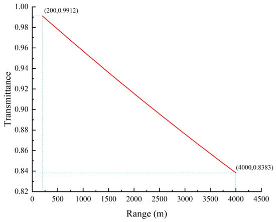
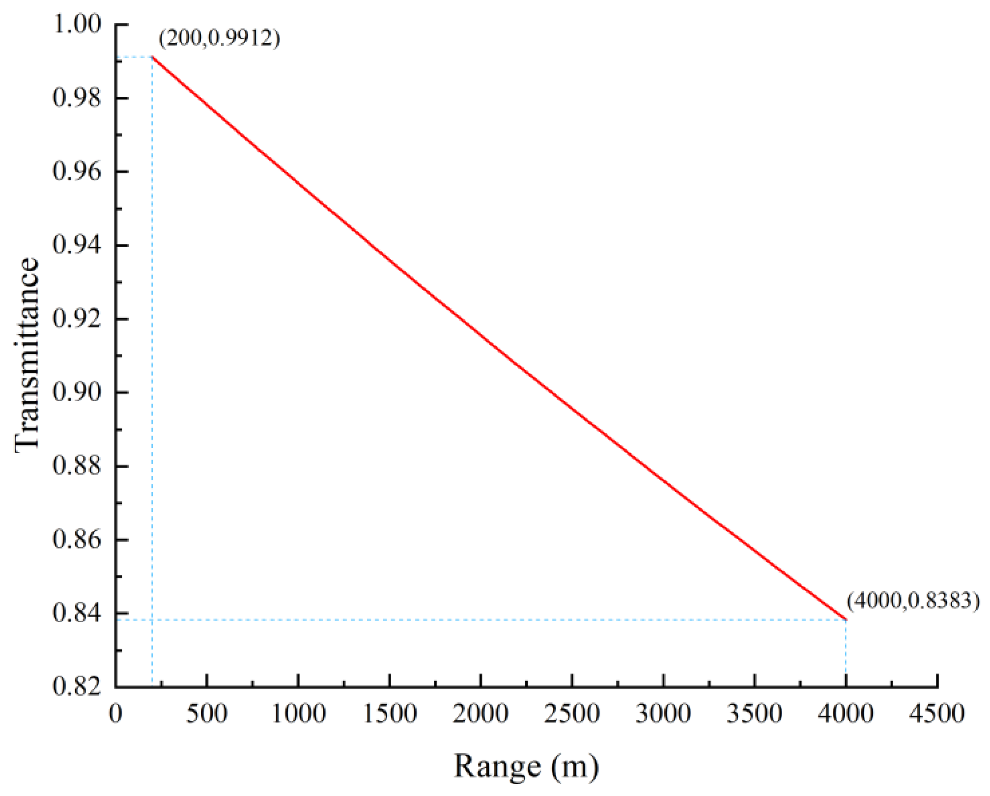
The calculation results for atmospheric transmittance are shown in Figure 7.

Figure 7. Atmospheric transmittance calculation results.

From Figure 7, it can be observed that within a range of 4000 m, the atmospheric transmittance and distance approximate a linear function relationship. However, when the distance extends to the 100 km scale, a distinct negative exponential relationship between atmospheric transmittance and distance becomes evident (see reference [29]). MATLAB (version R2024a) software was employed to fit the atmospheric transmittance data at various distances calculated by MODTRAN. Two types of fitting functions were selected for this study: $y=A{e}^{-\alpha R}$ and $y=A{e}^{-\alpha R}+B{e}^{-\beta R}$. The fitting results revealed that the coefficient of determination $R^2$ for both forms was approximately 1. Therefore, to simplify calculations, the first fitting form was adopted. The derived relationship between ${\tau }_{\alpha }$ and R is expressed as

$${\tau }_{\alpha }=e^{-4.409\times {10}^{-5}R}$$

(30)

The lidar was used to detect jet skis. The jet skis started moving from the lakeside close to the lidar and gradually moved away from it. The lidar’s built-in host computer software was used for distance calculation and real-time point cloud image display. By observing the position changes of the jet skis in the point cloud, the distance between the jet ski and the lidar was recorded at the moment the jet ski image disappeared. This distance represents the maximum operating range of the lidar for the jet ski.

4.2.2. Noise Analysis of Lidar

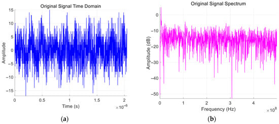
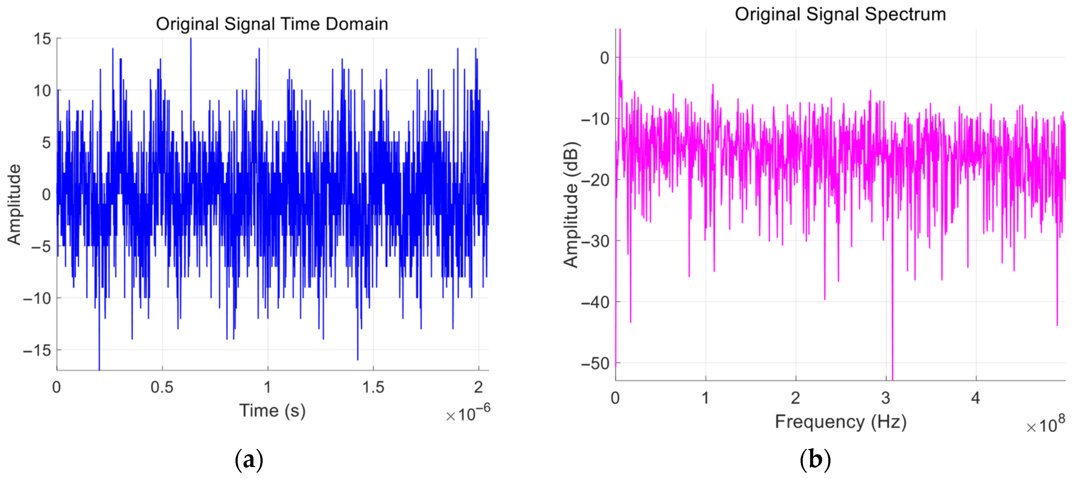
The electrical signals from the FMCW lidar detector are directly exported and processed using MATLAB software to analyze the noise characteristics of the system. The echo signal of the lidar is illustrated in Figure 8.

Figure 8. Original signal plots. (a) Time-domain plot; (b) Frequency spectrum plot.

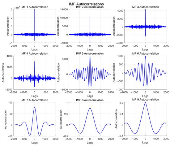
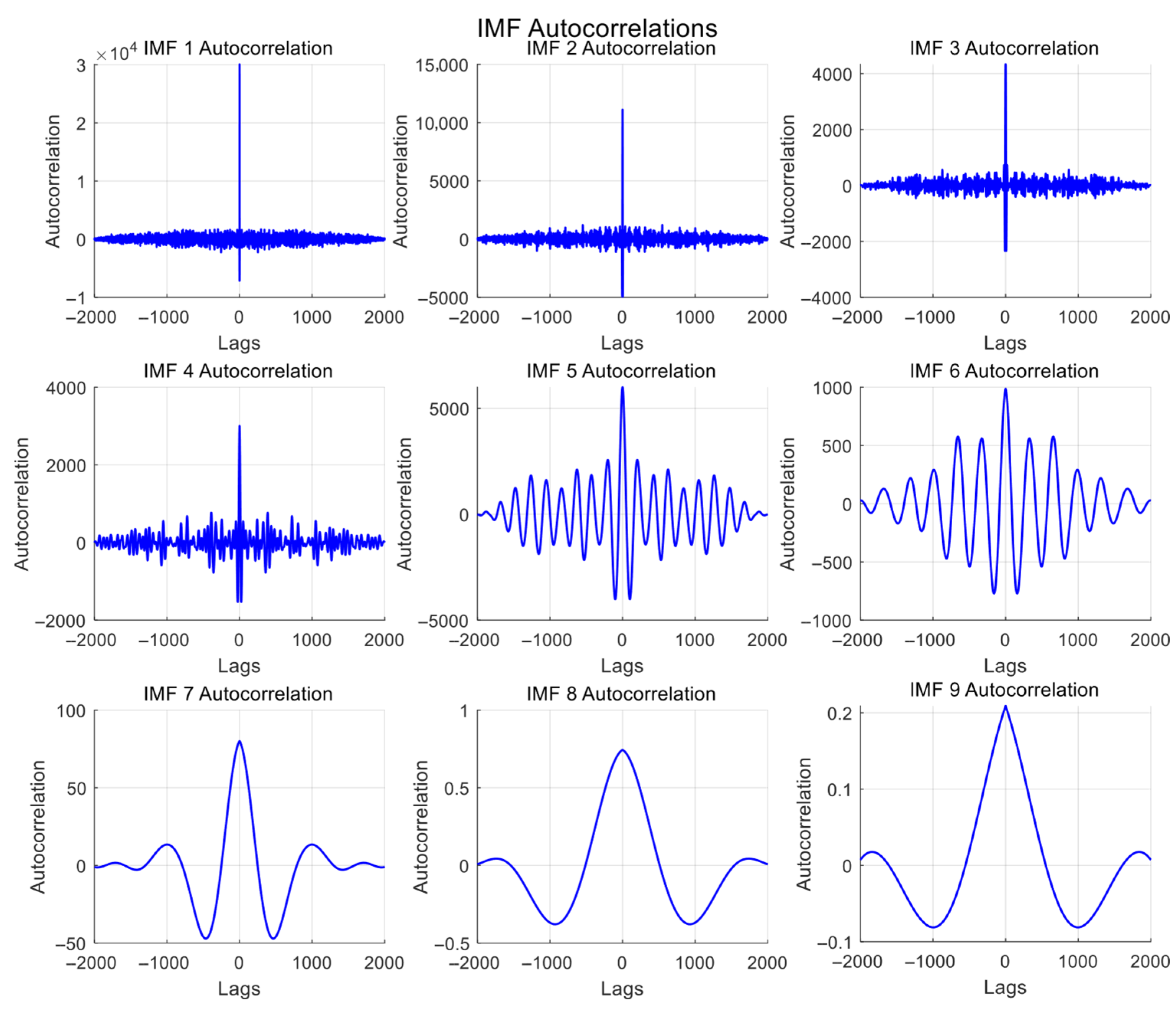
By applying Empirical Mode Decomposition (EMD) processing to the lidar output signal, the autocorrelation functions of each Intrinsic Mode Function (IMF) are obtained, as depicted in Figure 9. The x-axis represents the step size of time delay, while the y-axis represents the original autocorrelation values. Each IMF corresponds to signals within different frequency ranges, with IMF1 representing the highest frequency component of the signal, followed by sequentially lower frequencies, and the last IMF corresponding to the lowest frequency component of the signal.

Figure 9. Waveform plot of IMF autocorrelation functions.

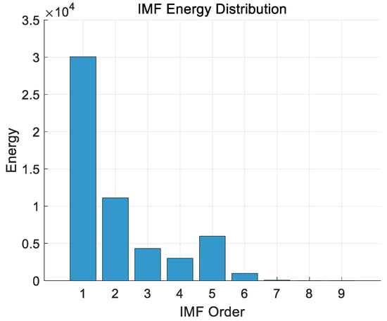
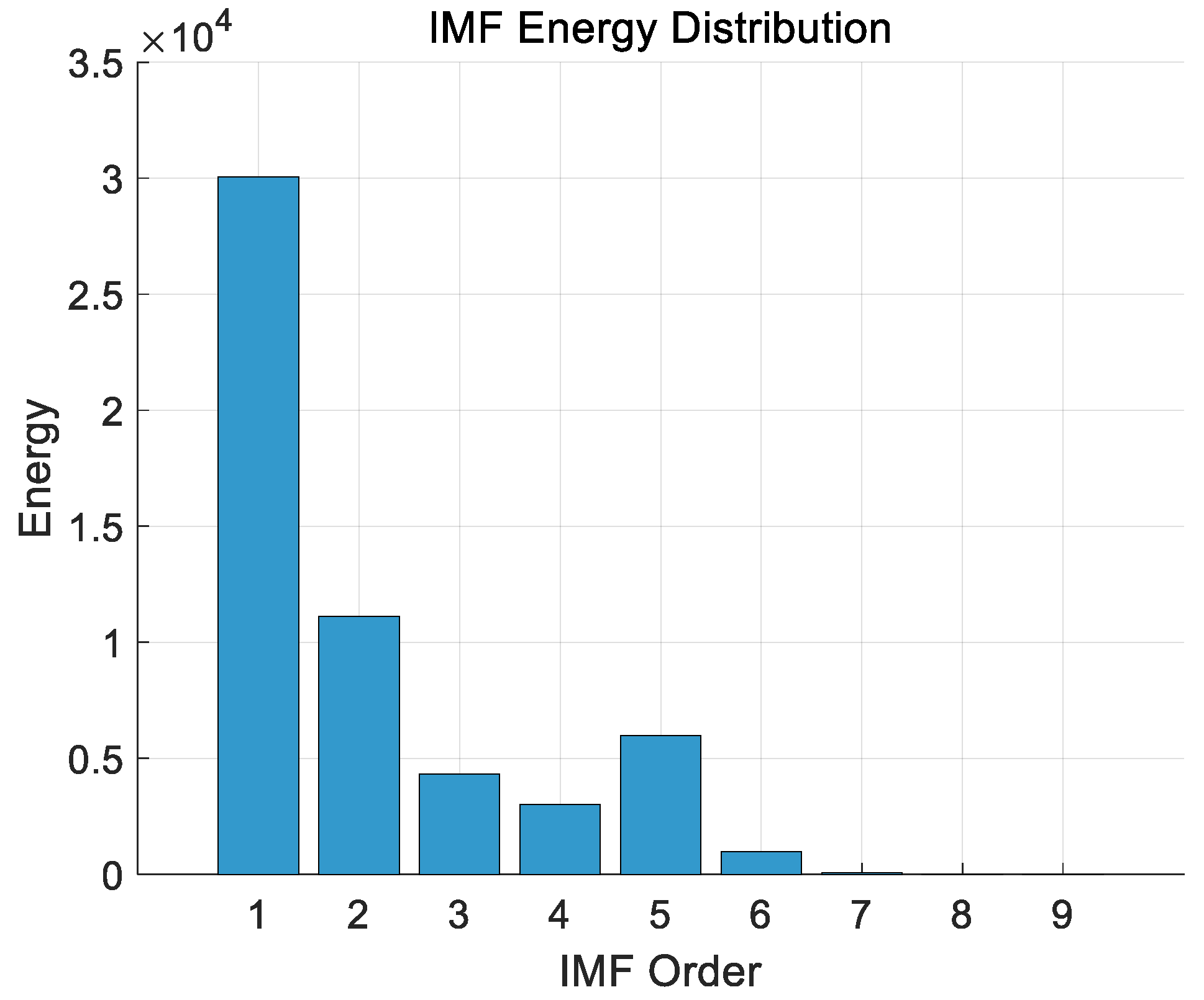
The energy distribution of each IMF is shown in Figure 10.

Figure 10. Energy distribution plot of IMFs.

The waveform of the IMF autocorrelation function reflects the linear correlation of the signal at different time lags. The autocorrelation function of a genuine signal typically exhibits distinct peaks, periodicity, or decaying oscillations, whereas the autocorrelation of noise usually manifests as random fluctuations near zero or rapid decay. Specifically, Gaussian noise, lacking temporal correlation, corresponds to an impulse function in the autocorrelation function of its high-frequency IMFs. In contrast, the IMF plots of low-frequency noise exhibit small-amplitude oscillatory variations along a certain axis of symmetry. Therefore, genuine signals and noise can be distinguished based on the auto-correlation function plots. From Figure 9, it can be observed that the waveform plots of IMF1–IMF3 exhibit sharp peaks only at zero time lag, with autocorrelation values close to zero and minimal fluctuations elsewhere. According to Figure 10, the first three IMFs account for the vast majority of the energy in the detector’s output signal. The waveform plots of IMF4 and IMF5 demonstrate pronounced oscillatory decay characteristics, featuring a prominent main peak at zero time lag followed by gradually decaying oscillations on both sides, indicating the presence of genuine signals in their autocorrelation functions. The waveform plots of IMF6–IMF9 exhibit small-amplitude oscillatory variations along the axis of symmetry, suggesting that they primarily comprise the low-frequency components of noise.

Through an analysis of the detector’s output noise, it can be concluded that the noise in the FMCW lidar system can be treated as Gaussian noise, consistent with the noise analysis conducted in Section 3.1.

By removing the intermediate frequency signal from the raw detection data of the FMCW lidar and performing noise calculations, the average total noise power is obtained as $P_N=6.4871\times {10}^{-7}\mathrm{W}$.

The raw signals from the lidar can undergo further noise reduction within the signal processing system. Commonly used noise reduction algorithms include Empirical Mode Decomposition (EMD) [30,31], Ensemble Empirical Mode Decomposition (EEMD) [32], Variational Mode Decomposition (VMD) [33], Singular Spectrum Analysis (SSA) [34], among others. Utilizing these noise reduction algorithms can further enhance the signal-to-noise ratio (SNR) of the raw signals. The Empirical Mode Decomposition combined with Wavelet Transform (EMD-WT) joint denoising algorithm adopted in this study can elevate the SNR of a raw signal with an initial SNR of 17.33 dB to a maximum of 30.09 dB (see reference [35]). For automotive FMCW lidars, signals with an SNR greater than 10 dB after processing are typically considered valid and output as point clouds. The lidar used in this study corresponds to a 3 dB SNR threshold before noise reduction, i.e., the threshold SNR $R_{SN}^{\prime }=3\mathrm{dB}$.

4.2.3. Experimental Results

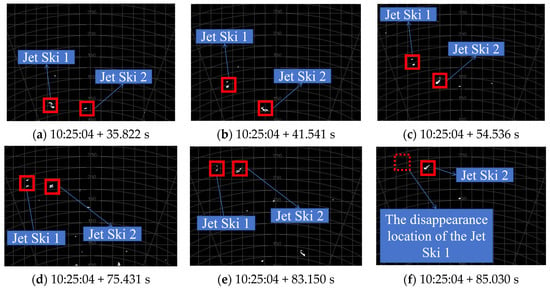
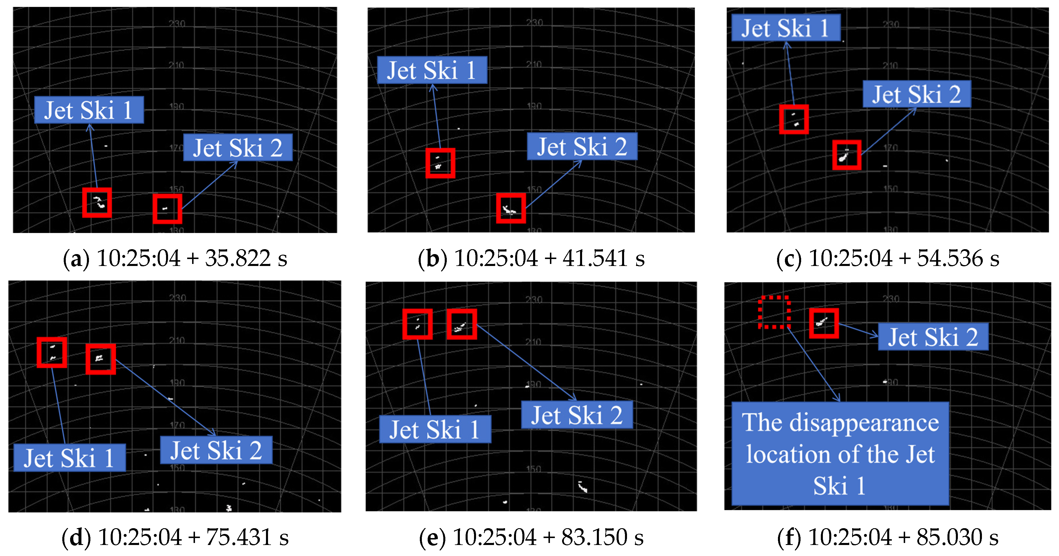
Timing commenced from the moment the lidar was powered on, and the positional changes of the jet ski in the point cloud map, along with the corresponding times, were recorded. The jet ski’s motion was displayed in real-time within the lidar’s ac-companying point cloud software, as illustrated in Figure 11. Figure 11 simultaneously displays both the Cartesian and polar coordinate systems established with the lidar as the origin, represented by grid lines and circular lines, respectively. The numbers on the circular scale lines indicate the distances from those lines to the lidar. When the lidar’s echo signal falls below the threshold SNR, the point cloud signal disappears; conversely, when the echo signal exceeds the threshold SNR again, the point cloud signal reappears automatically. By recording the positions where the jet ski’s point cloud signal disappears or reappears, the maximum operating range of the lidar can be determined.

Figure 11. Jet ski motion.

Figure 11 shows that at 183.2 s, the lidar echo signal disappeared from the point cloud, and the recorded jet ski distance information was 230.24 m.

To ensure experimental accuracy, the jet ski moved repeatedly at the position where it first disappeared, and the positions and times when the jet ski image disappeared and appeared each time were recorded. The recorded data are shown in Table 3.

Table 3. Field test results.

Time/s	Appear/Disappear	Measured Distance/m
10:28:57 + 18.320	Disappear	228.95
10:28:57 + 40.925	Appear	236.76
10:32:17 + 26.251	Disappear	251.12
10:32:17 + 41.683	Appear	246.06
10:32:17 + 58.252	Disappear	249.27
10:32:17 + 98.353	Appear	254.22
10:35:37 + 17.421	Disappear	275.54
10:35:37 + 33.686	Appear	276.05
10:35:37 + 54.376	Disappear	242.01
10:35:37 + 78.945	Appear	244.32

The experimental measurement average was 250.43 m. Among the experimental measurements, the distance exceeded 270 m twice because of changes in the area of the jet ski illuminated by the laser: when the bow or stern of the jet ski faced the lidar, at relatively far distances, the number of point clouds for the jet ski was small and might be filtered out as noise points during point cloud processing. At this time, the maximum distance measured by the lidar fluctuated at around 230–250 m. When the side of the jet ski faced the lidar, the number of point clouds would increase, and the maximum distance measured by the lidar would exceed 270 m.

Considering point cloud processing factors, when the jet ski moved to about 270 m from the shore, its direction was adjusted to keep the distance between the jet ski and the shore constant, moving only horizontally to the left (or right). The positions and times when the jet ski image disappeared and appeared each time were recorded, with data shown in Table 4.

Table 4. Test results during horizontal jet ski movement.

Time/s	Appear/Disappear	Measured Distance/m
10:40:42 + 20.354	Disappear	276.36
10:40:42 + 27.740	Appear	277.56
10:40:42 + 53.525	Disappear	275.37
10:40:42 + 59.141	Appear	273.92
10:45:02 + 20.364	Disappear	271.09
10:45:02 + 29.829	Appear	270.30
10:45:02 + 50.683	Disappear	272.45
10:45:02 + 61.573	Appear	270.73
10:49:22 + 06.778	Disappear	268.77
10:49:22 + 15.336	Appear	268.32

The experimental measurement average was 272.49 m. During the experiment, when the jet ski remained stationary at the position where it appeared, the lidar could continuously identify the target. However, when the jet ski started moving, there was a certain probability of it being filtered out as noise points at closer distances. This indicates that target motion affects the maximum ranging capability of FMCW lidar: the lidar’s operating range for stationary targets is relatively long, but the difference with the operating range for moving targets is insignificant. This is because the jet ski’s motion speed was small, so its impact on the operating range was also small.

Substituting the parameters of the FMCW lidar, the average noise power, and the atmospheric transmittance into Equation (28) yields an implicit function equation only in terms of R. Using Newton’s method for iterative solution yields $R=293.60$ m, with a relative error of 7.74% compared with the measured value.

5. Conclusions

Based on the optical mixing principle and FMCW lidar ranging principle, and considering that existing FMCW lidar systems use couplers for optical mixing and balanced photodetectors for detection, this study derives an FMCW lidar ranging equation and analyzes the calculation of various parameters. Example calculations using the operating range model were performed to verify the model’s reliability. We draw the following conclusions:

• Compared with the traditional lidar equation, the FMCW lidar range equation incorporates coherent gain, G, fully considering the influence of LO light on the operating range. After introducing coherent gain, G, for extended targets, the operating range, R, is inversely proportional to noise power and the signal-to-noise ratio, whereas in the traditional lidar range equation, the square of operating range R is inversely proportional to noise power and signal-to-noise ratio. Therefore, noise power has a greater impact on the operating range. For laser output power, the FMCW lidar equation is consistent with the general lidar equation; both are proportional to it when ranging extended targets.
• Lidar point cloud generation also affects the operating range. When the target area is small with only limited point cloud information, the points generated by weak echo signals may be filtered out as noise points. Larger targets can return more point clouds and thus will not be filtered out, resulting in a longer operating range.
• Target motion characteristics also affect the radar’s operating range. Our experiments demonstrate that the operating range for stationary targets is relatively long.

FMCW lidar has wide applications in fields such as autonomous driving and unmanned aerial vehicles (UAVs). Since optical mixing has higher sensitivity and stronger anti-interference capability than electrical mixing, current FMCW lidar systems typically employ optical mixing combined with balanced photodetectors for detection. The FMCW lidar ranging equation based on optical mixing can estimate operating ranges for various commonly used FMCW lidar systems, thereby enabling better performance evaluation. The operating range equation indicates that the operating range of FMCW lidar is significantly affected by the target and the on-site environment. Therefore, FMCW lidar systems must be optimized considering specific application scenarios.

The derived operating range equation in this paper still has certain limitations: Firstly, it does not account for the impact of the point cloud generation algorithm on operating range. When generating point clouds from signals processed by FFT, some isolated target points may be treated as noise, thereby shortening the effective operating range. Secondly, the equation does not address scenarios involving highly dynamic motion, making it more suitable for detecting stationary or low-speed targets. In addition, water exhibits strong absorption of laser light at a wavelength of 1550 nm, resulting in relatively minimal environmental interference during experiments involving surface targets. Subsequent research will delve further into lidar point cloud processing and target Doppler shift analysis, as well as design lidar detection experiments under various environmental conditions to investigate their effects on the operating range of FMCW lidar.

References

- Lu, Z.Y.; Ge, C.F.; Wang, Z.Y.; Jia, D.F.; Yang, T.X. Basics and developments of frequency modulation continuous wave LiDAR. Opto-Electron. Eng. 2019, 46, 7–20. [Google Scholar] [CrossRef]
- Martin, A.; Verheyen, P.; De Heyn, P.; Absil, P.; Feneyrou, P.; Bourderionnet, J.; Dodane, D.; Leviandier, L.; Dolfi, D.; Naughton, A.; et al. Photonic integrated circuit-based fmcw coherent lidar. J. Light. Technol. 2018, 36, 4640–4645. [Google Scholar] [CrossRef] [Scilit]
- Royo, S.; Ballesta-Garcia, M. An overview of lidar imaging systems for autonomous vehicles: 19. Appl. Sci. 2019, 9, 4093. [Google Scholar] [CrossRef] [Scilit]
- Ke, J.-Y.; Song, Z.-Q.; Wang, P.-S.; Cui, Z.-M.; Mo, D.; Lin, M.; Wang, R.; Wu, J. Long distance high resolution fmcw laser ranging with phase noise compensation and 2d signal processing. Appl. Opt. 2022, 61, 3443. [Google Scholar] [CrossRef] [Scilit]
- Xiao, Z.; Wu, Z.; Xia, G. Phase-noise-cancelled fmcw lidar based on cs-dsb modulation and injection-locking technique. Opt. Laser Technol. 2024, 168, 109936. [Google Scholar] [CrossRef] [Scilit]
- Sun, Y.; Xing, X.; Li, W.; Wang, J.; Hu, P.; Tan, J. A high-accuracy, high-speed dynamic performance test method for heterodyne interferometry measurement electronics. IEEE Trans. Instrum. Meas. 2024, 73, 1–8. [Google Scholar] [CrossRef] [Scilit]
- Pinto, L.C.P.; Medeiros, M.C.R. Enhanced high-resolution and long-range fmcw lidar with directly modulated semiconductor lasers. Sensors 2025, 25, 4131. [Google Scholar] [CrossRef] [Scilit]
- Norton, K.A.; Omberg, A.C. The maximum range of a radar set. Proc. IRE 1947, 35, 4–24. [Google Scholar] [CrossRef] [Scilit]
- Li, C.L.; Liu, J.C.; Zhang, F.M.; Qu, X.H. Review of nonlinearity correction of frequency modulated continuous wave LiDAR measurement technology. Opto-Electron. Eng. 2022, 49, 210438. [Google Scholar] [CrossRef]
- Shipley, S.T.; Tracy, D.H.; Eloranta, E.W.; Trauger, J.T.; Sroga, J.T.; Roesler, F.L.; Weinman, J.A. High spectral resolution lidar to measure optical scattering properties of atmospheric aerosols. 1: Theory and instrumentation. Appl. Opt. 1983, 22, 3716–3724. [Google Scholar] [CrossRef] [Scilit]
- Karlsson, C.J.; Olsson, F.Å.A. Linearization of the frequency sweep of a frequency-modulated continuous-wave semiconductor laser radar and the resulting ranging performance. Appl. Opt. 1999, 38, 3376. [Google Scholar] [CrossRef] [Scilit] [PubMed]
- Chen, D.; Wang, J.G.; Kang, S. Lidar Equation Amending in Dense Media Based on Double Scattering Approximation. In Proceedings of the 2010 National Vocational Education of Communications and Information Technology Conference (2010 NVCIC), Rizhao, China, 4–5 December 2010; Available online: https://kns.cnki.net/kcms2/article/abstract?v=Mz9udXFtQxkXrJfu0CjWcy4fQFkr4KpVOSXKo00OngL19ZH7DH8CW-gVZDSONJ2ZVPay4HOV2yjjdbNn2nZ1d7JqdmO3n-Ffzalh2gJLIltyYND05gzbn2v9EmGciOGvfRelxJ1s2_bQ6AO9ggAHOMiqCudUHqjKoQUkUnmaV3r89BQBsIB_Ow==&uniplatform=NZKPT&language=CHS (accessed on 20 October 2025).
- Wang, T.; Sun, J.; Wang, X.; Wang, Q. Improvement and simulation of flash focal plane lidar equation. Infrared Laser Eng. 2012, 41, 626–631. [Google Scholar]
- Yang, H.Z.; Zhao, C.M.; Zhang, H.Y.; Yang, S.H.; Zheng, Z.; Zheng, X.Y.; Zhang, D.H. Design and Optimization of All-Fiber Lidar Transmitting and Receiving Optical Systems. Acta Opt. Sin. 2016, 36, 65–72. [Google Scholar] [CrossRef] [Scilit]
- Siddiq, K.; Hobden, M.K.; Pennock, S.R.; Watson, R.J. Phase noise in fmcw radar systems. IEEE Trans. Aerosp. Electron. Syst. 2019, 55, 70–81. [Google Scholar] [CrossRef] [Scilit]
- Cha, K.; Oh, S.; Hong, H.; Park, H.; Hong, S.K. Detection of electronic devices using fmcw nonlinear radar. Sensors 2022, 22, 6086. [Google Scholar] [CrossRef] [Scilit]
- Putra, B.P.H.; Akbar, F.S.; Untsa, R.M. Maximum range analysis of an sdr-based fmcw radar. In Proceedings of the 2024 IEEE 22nd Student Conference on Research and Development (Scored), Selangor, Malaysia, 19–20 December 2024. [Google Scholar] [CrossRef] [Scilit]
- Lin, H.Z.; Shi, S.; Wang, L.C.; Zhou, Y.Z. Scattering characteristics of Gaussian random rough surface targets and their influence on the parameters of the LiDAR equation. Acta Opt. Sin. 2025, 45, 2. Available online: https://www.opticsjournal.net/Articles/g251143/EarlyPosting (accessed on 20 October 2025).
- Melvin, W.L.; Scheer, J. (Eds.) Principles of Modern Radar: Advanced Techniques; Institution of Engineering and Technology: Stevenage, UK, 2012. [Google Scholar] [CrossRef] [Scilit]
- Tong, Y.T. Research on Photonics-Based Genration and Receiving Processing of Radar Signals Based on Phase-Locked Dual Optical Frequency Combs. Master’s Thesis, Shanghai Jiao Tong University, Shanghai, China, 2019. Available online: https://kns.cnki.net/kcms2/article/abstract?v=4qE7rfs4XRFfAKW2wDNY7w1zY5YR7zaEMA1m7fWGstbK12p-kq9TTXKh8iEFTsfSjV3Mrqh5-r1q5oeQPcJTn2rHzCKqGFiXVPQ0czD6cCxWOXNBzgMxorsLXuWrCci9EDOCHX0ACapgn8GRSxOz1SDlCE2xTcCyG2imMaEBTWuUwTTOJ_VM0a10Rrq5Dvjn&uniplatform=NZKPT&language=CHS (accessed on 13 November 2025).
- Nicodemus, F.E. Directional reflectance and emissivity of an opaque surface. Appl. Opt. 1965, 4, 767–775. [Google Scholar] [CrossRef] [Scilit]
- Steinvall, O. Effects of target shape and reflection on laser radar cross sections. Appl. Opt. 2000, 39, 4381–4391. [Google Scholar] [CrossRef] [Scilit]
- Oppenheim, A.V.; Willsky, A.S.; Nawab, S.H. Signals and Systems, 2nd ed.; Prentice Hall: Old Tappan, NJ, USA, 1997; ISBN 0-13-814757-4. [Google Scholar]
- Proakis, J.G.; Salchi, M.; Proakis, J. Digital Communications, 5th ed.; McGraw-Hill Education: Columbus, OH, USA, 2007; ISBN 9780072957167. [Google Scholar]
- Batet Torrell, Ó. Investigation of Continuous-Wave Range-Resolved Lidar Systems for Gas Detection and Concentration Measurement. Ph.D. Thesis, Universitat Politècnica de Catalunya, Barcelona, Spain, 2011. [Google Scholar] [CrossRef] [Scilit]
- Siddiq, K. The Impact of Oscillator Phase Noise on the Design of Millimetre-Wave Continuous Wave Radar Systems. Ph.D. Thesis, University of Bath, Bath, UK, 2017. Available online: https://purehost.bath.ac.uk/ws/portalfiles/portal/187919059/SIDDIQ_PhDThesis_.pdf (accessed on 15 January 2026).
- Siddiq, K.; Watson, R.J.; Pennock, S.R.; Avery, P.; Poulton, R.; Dakin-Norris, B. Phase noise analysis in fmcw radar systems. In Proceedings of the 2015 European Microwave Conference (EuMC), Paris, France, 7–10 September 2015. [Google Scholar] [CrossRef] [Scilit]
- Yang, W.H.; Zhang, P.; Yang, X.F.; Chen, Q.M.; Zhao, W. Performance Optimization and Experimental Research of Continuous Wave Coherent Wind Lidar. Acta Photonica Sin. 2021, 50, 0401004. [Google Scholar] [CrossRef] [Scilit]
- Sun, C.; Yang, B.; Sun, J. An netd-based optimization model for the operating range of a staring infrared system. Appl. Sci. 2025, 15, 10746. [Google Scholar] [CrossRef] [Scilit]
- Liu, Z.; Wu, J.; Yang, S.; Lu, W. DOA estimation method based on emd and music for mutual interference in fmcw automotive radars. IEEE Geosci. Remote Sens. Lett. 2022, 19, 1–5. [Google Scholar] [CrossRef] [Scilit]
- Wang, Y.; Gao, D.; Xu, X.; Liao, G.; Zeng, H.; Yue, Y. Interference suppression for fmcw radars with emd enhanced sparse matrix recovery. In 2024 IEEE International Conference on Signal, Information and Data Processing (ICSIDP); IEEE: Piscataway, NJ, USA, 2024. [Google Scholar] [CrossRef] [Scilit]
- Li, Z.; Wang, N.; Li, Y.; He, J.; Zhao, Y. A novel fmcw lidar multi-target denoising method based on optimized ceemdan with singular value decomposition. Electronics 2025, 14, 2697. [Google Scholar] [CrossRef] [Scilit]
- Gaur, A.; Tseng, P.-H.; Feng, K.-T.; Srirangarajan, S. Signal decomposition based mutual interference suppression in fmcw radars. IEEE Open J. Veh. Technol. 2025, 6, 2677–2692. [Google Scholar] [CrossRef] [Scilit]
- Wu, Z.; Liu, H.; Ma, C.; Liu, Z. Aerial target recognition with enhanced micro-doppler dynamic features based on frequency-modulated continuous-wave radar. IEEE Sens. J. 2023, 23, 23119–23132. [Google Scholar] [CrossRef] [Scilit]
- Sun, J.; Sun, C.; Yang, B. FMCW lidar signal processing using emd and wavelet transform for gaussian noise suppression. Appl. Sci. 2025, 16, 256. [Google Scholar] [CrossRef] [Scilit]
Disclaimer/Publisher’s Note: The statements, opinions and data contained in all publications are solely those of the individual author(s) and contributor(s) and not of MDPI and/or the editor(s). MDPI and/or the editor(s) disclaim responsibility for any injury to people or property resulting from any ideas, methods, instructions or products referred to in the content. |
© 2026 by the authors. Licensee MDPI, Basel, Switzerland. This article is an open access article distributed under the terms and conditions of the Creative Commons Attribution (CC BY) license.