


Abstract
This paper addresses the Pickup and Delivery Problem with Time Windows (PDPTW), an NP-hard combinatorial optimization problem with major practical relevance in logistics and transportation. The study focuses on a quadratic unconstrained binary optimization (QUBO) formulation for quantum annealing and benchmarks it against two classical optimization paradigms. A modular Python framework is developed that encodes PDPTW in three ways: a mixed-integer linear programming (MILP) model that serves as an exact reference, a genetic algorithm (GA) metaheuristic, and a QUBO model that is compatible with quantum annealers. The framework supports test scenarios with increasing structural complexity, with both feasible and intentionally infeasible instances. An additional contribution is the conceptual design and preliminary analysis of an automatic-penalty weight-tuning scheme for the QUBO model. Experimental results show that the proposed QUBO formulation can produce high-quality solutions for simpler PDPTW instances, but its performance strongly depends on the careful calibration of penalty weights. MILP provides optimal baselines on small instances but becomes intractable as problem size grows. The GA scales to the largest scenario and finds feasible solutions of reasonable quality, but they are not necessarily optimal. The evaluation also includes a large number of problem instances and runs on IBM Quantum hardware using the Quantum Approximate Optimization Algorithm (QAOA).
1. Introduction
The current transport market faces high volatility, frequent changes in demand patterns, and strong competition at both local and global levels. Logistics optimization is essential for maintaining operational efficiency and competitiveness for companies that depend on freight transport operations. Route planning, allocation of fleet resources, and strict adherence to customer and operational requirements (including time and cost constraints) lead to complex decision problems.
This paper focuses on the Pickup and Delivery Problem with Time Windows (PDPTW), an NP-hard combinatorial optimization problem that arises as a variant of the Vehicle Routing Problem with Pickup and Delivery (VRPPD) [1,2,3]. In PDPTW, each transportation request consists of a pickup location and a corresponding delivery location that must be served by the same vehicle, under a precedence constraint that enforces pickup before delivery. Vehicles operate under capacity constraints and must respect time windows of customers. Dynamic variants, in which requests appear over time and require online re-optimization, are surveyed in [4], which discusses insertion heuristics and waiting strategies that are essential when exact methods become impractical in real time. In this paper, we focus on a static, deterministic PDPTW in which all pickup–delivery requests are known in advance. The aim is not to reflect all the features of real-world logistics, but to focus on a core version of the problem that allows for a clear comparison between solution paradigms and an exploration of what is currently feasible on quantum hardware.
The NP-hardness of VRPPD and PDPTW [1] limits the scalability of exact methods such as mixed-integer linear programming (MILP): they can provide optimal solutions for small instances but often become intractable for larger ones [5,6]. Practical applications and much of the literature therefore rely on heuristic and metaheuristic approaches. Genetic algorithms (GAs) are a prominent example; they use population-based evolutionary operators to explore large search spaces and often find high-quality solutions but do not provide guarantees of global optimality [7,8].
Quantum computing offers an alternative approach to hard combinatorial optimization problems that remain difficult to solve on a large scale. A central paradigm in this context is the reformulation of such problems as Quadratic Unconstrained Binary Optimization (QUBO) models, which encode objectives and constraints into a unified quadratic binary form [9,10]. QUBO models are directly compatible with quantum annealing hardware, and they also serve as the input format for many variational quantum algorithms such as the Quantum Approximate Optimization Algorithm (QAOA) and the Variational Quantum Eigensolver (VQE), which can be executed on quantum devices or classically simulated through frameworks such as Qiskit [11]. Applications of QUBO formulations to routing problems are promising [12], yet they still face significant challenges related to constraint encoding and the calibration of penalty parameters. The practical relevance of PDPTW continues to grow through applications that involve dynamic and heterogeneous constraints [6].
This study investigates a QUBO formulation of the PDPTW that is suitable for quantum annealing and evaluates its performance in comparison with two classical approaches: an exact MILP model and a genetic algorithm. The focus is on building a compact QUBO model for this fundamental variant, rather than proposing a new industrially detailed formulation. While the modeling elements themselves are fairly standard, the formulation combines bit-length tuning and scaling in a way that reduces auxiliary variables and clarifies the trade-offs between model size and constraint strength. The QUBO model is designed to be compatible with quantum annealers and is solved here in two ways. First, an offline solver from D-Wave is used, which applies classical heuristic algorithms to the same QUBO formulation as on the quantum hardware. Second, proof-of-concept executions are run on a real quantum computer. A benchmark suite of 27 synthetic PDPTW instances is employed, which systematically varies problem size, customer distribution, and time-window tightness, in order to analyze how the QUBO formulation scales under classical simulation. Selected small instances are executed on IBM Quantum hardware using QAOA, which demonstrates that the same QUBO formulation can run on a gate-based processor and provides an initial quantitative comparison between classical simulated annealing and quantum optimization for PDPTW. The MILP formulation serves as an exact baseline for small instances and is implemented and solved with a specialized MILP solver. The GA serves as a metaheuristic baseline that can handle larger instances, but its solutions are not necessarily optimal. The comparative analysis aims to clarify the strengths and limitations of each approach on a common set of PDPTW test scenarios.
The paper follows these specific objectives:
- 1.
- To develop and implement a detailed QUBO formulation for the PDPTW that captures the relevant constraints and uses a dynamic mechanism for determining the number of auxiliary binary variables;
- 2.
- To implement a GA tailored to the PDPTW, with appropriate chromosome representation, selection, crossover, and mutation operators, and a penalty-based fitness function to handle constraints;
- 3.
- To construct a reference MILP model for the PDPTW and solve it using a specialized optimization solver;
- 4.
- To generate and validate a heterogeneous set of test instances with varying sizes and structural complexity, including both feasible and intentionally infeasible cases inspired in part by the literature [8];
- 5.
- To carry out a systematic experimental study for the three methods;
- 6.
- To perform a comparative analysis of the obtained results in terms of feasibility, solution quality, and computational time for each test case, and to assess the practical implications for current quantum hardware.
The methodology combines theoretical analysis, mathematical modeling, software implementation, and experimental evaluation. Section 2 reviews related work on QUBO models, GAs, and MILP approaches for routing problems. Section 3 formally defines the PDPTW and presents the mathematical model, including decision variables, objective function, and constraints. Section 4 describes the three implemented solution approaches: the QUBO model with its penalty-weight adjustment mechanism, the GA tailored to PDPTW, and the MILP reference model. Section 5 presents the experimental study, including the test instances, the results of each method, and a comparative discussion of their performance. Section 6 summarizes the conclusions, highlights the main contributions, and outlines directions for future research.
2. Related Work
Research on the Vehicle Routing Problem with Pickup and Delivery (VRPPD) and its time-window variant (PDPTW) covers both practical logistics applications and methodological developments in exact, heuristic, and quantum-inspired approaches. This section reviews recent work on VRPPD and PDPTW, with emphasis on MILP and related exact methods, metaheuristics such as GAs, and QUBO-based or quantum optimization approaches. We aim to position our comparative study relative to state-of-the-art formulations and solution techniques.
2.1. VRPPD with Time Windows: Exact Formulations and Robust Methods
The Pickup and Delivery Problem with Time Windows (PDPTW) is one of the most extensively studied VRPPD variants, and recent years have seen significant progress in exact and robust formulations that capture realistic operational constraints.
Deng et al. [13] study cold chain transportation for perishable products under incompatibility constraints. They propose a branch-and-price algorithm based on a set-partitioning formulation, where each column represents a feasible route that satisfies capacity, time windows, and temperature-compatibility restrictions. The objective combines distance, refrigeration costs, and quality degradation. Computational experiments on real-world data report total cost reductions of 15–20% compared to distance-only optimization, which underscores the value of integrated modeling for PDPTW-like problems.
Wang et al. [14] consider a PDPTW with hard time windows and stochastic, time-dependent travel times (PDPHTW-STDTT). They adopt a scenario-based robust formulation that enforces time-window feasibility with a prescribed probability level. A branch-cut-and-price algorithm solves the resulting model, with specialized cutting planes and dominance rules in the pricing subproblem. The robust solutions exhibit service reliability above 95% under adverse traffic conditions, at the cost of an 8–12% increase in total cost compared to deterministic models, which frequently violate time windows.
Electric vehicle routing adds battery and charging constraints to the PDPTW structure. Liu et al. [15] propose a two-stage robust optimization framework for EV-PDPTW with uncertain demands. First-stage decisions fix routes and schedules, and second-stage recourse decisions adjust transported quantities after demand realization, under a Bertsimas–Sim budget uncertainty set. A column-and-row generation algorithm with an adversarial separation subproblem solves the model. For instances up to 50 requests, the robust approach maintains feasibility in about 98% of demand realizations with only a 3–5% cost increase over deterministic solutions, and performs markedly better under high demand variability.
Praxedes et al. [16] introduce a unified framework, denoted HLRPSPDTW, that accommodates multiple routing features in a single model, including heterogeneous fleets, time windows, route duration limits, multiple depots, and facility location decisions. They derive an extended set-partitioning formulation and solve it via branch-cut-and-price, with bucket-based labeling, ng-sets, and limited-memory cuts to control state-space growth. On more than 550 benchmark instances that cover ten VRPSPD and PDPTW variants, the unified algorithm matches or improves specialized approaches and identifies 47 new optimal solutions.
Abreu et al. [17] address the simultaneous uncertainty in demands and travel times in a robust PDPTW model. The formulation uses cardinality-bounded uncertainty sets for both demand and travel time, and it is solved with a branch-and-cut algorithm that dynamically generates robust cuts through separation procedures. Monte Carlo simulations on 1000 joint realizations show feasibility rates above 99.5% for the robust solutions, compared to 65–75% for deterministic solutions, with cost premiums in the range of 4–7%.
2.2. VRPPD with Simultaneous Pickup and Delivery and a Capacitated Fleet
Simultaneous pickup and delivery settings extend classical VRPPD by allowing vehicles to deliver goods from the depot and collect items from customers on the same routes. This setting appears in many distribution systems where backhauls matter as much as outbound flows and where capacity constraints strongly influence route design.
Louati et al. [18] compare several MILP formulations for a real-life simultaneous pickup and delivery problem. They study an extended graph formulation with separate pickup and delivery nodes, a two-index flow formulation, and a three-index formulation. The numerical comparison shows that formulation choice strongly affects performance: the extended graph model solves small instances faster, while the more compact two-index formulation gives tighter relaxations and becomes preferable as instance size grows. This result underlines that even within exact approaches, modeling decisions have a major impact on solvability.
Metaheuristic methods must also address parameter tuning. Rüther et al. [19] use Bayesian optimization to tune a Grouping Genetic Algorithm (GGA) for multi-depot VRPPD with time windows and heterogeneous fleets. The GGA uses a grouping representation of requests and specialized operators that preserve group structure. The Bayesian layer treats algorithm performance as a black-box function of parameters and learns good configurations over time. On instances with 100–150 requests, automatically tuned GGA variants reduce total cost by 12–18% and use fewer vehicles than manually tuned baselines, with parameter settings that transfer well between instance classes.
Load splitting gives an additional degree of freedom. Gasque and Munari [20] study PDPTW with heterogeneous fleets and multiple product types, and allow a customer’s demand to be served by several vehicles. They develop an Adaptive Large Neighborhood Search (ALNS) that updates the weights of removal and insertion operators based on past performance. Experiments on instances with up to 150 customers show that enabling load splitting reduces total costs by 18–25% compared to non-split models, while fleet heterogeneity brings further improvements. The authors also release an open-source platform that supports the implementation and testing of these variants.
Sustainability concerns motivate “green” versions of the Vehicle Routing Problem with Simultaneous Pickup and Delivery (VRPSPD). Olgun et al. [21] introduce a Green VRPSPD where the objective focuses on fuel consumption and emissions rather than pure distance. They use a detailed fuel model that depends on distance, load, and speed, and they propose a hyper-heuristic ILS (HH-ILS) that selects and adapts low-level neighborhood operators. Results show fuel savings of about 5–10% and emission reductions of 8–12% compared to distance-minimizing solutions, with notable changes in route structure and vehicle utilization.
Product incompatibilities often arise in practice when certain goods cannot share vehicles for safety or quality reasons. Weerakkody et al. [22] study such constraints in a third-party logistics context with simultaneous pickup and delivery. Their heuristic first clusters compatible products, then designs routes within each group, and finally applies improvement moves that preserve incompatibility rules. A real case study shows a 30–40% reduction in the number of trips and about 15% distance savings compared to manual planning, while still respecting all incompatibility constraints.
2.3. Dynamic VRPPD, Ride-Sharing and Dial-a-Ride Services
Dynamic VRPPD and related dial-a-ride problems require decisions in real time as new requests arrive. Algorithms must update existing routes quickly and preserve flexibility for future requests, which leads to algorithmic designs that differ from those developed for static benchmarks.
Zhou et al. [23] address a dynamic pickup and delivery problem that arises in inter-factory logistics. They propose a memetic algorithm that combines a genetic component with local search. The population maintains alternative route sets, while local search improves individuals whenever new requests appear. The method accepts significantly more requests than greedy insertion heuristics (15–20% improvement) and reduces total cost by 8–12% on 64 real instances from Huawei’s operations.
Ackermann and Rieck [24] take a multiple-plan view of dynamic dial-a-ride problems. Instead of maintaining a single incumbent solution, their method keeps several alternative plans in parallel. Each new request is evaluated against all plans, and the best insertion position is chosen. Periodic rebalancing preserves diversity among plans and avoids premature convergence to one configuration. Experiments on ride-pooling scenarios show that five to eight concurrent plans increase request acceptance by 5–10% and reduce the average response time by 20–30% compared to single-plan strategies.
Recent work in passenger transport incorporates equity objectives alongside operating costs. Azi et al. [25] introduce an equity-aware dial-a-ride problem that balances operating cost with fairness in passenger travel times. They define an equity measure based on deviations from ideal direct travel times and embed it in a bi-objective formulation. A branch-cut-and-price algorithm generates routes that account for both cost and equity. Results on adapted benchmark instances indicate that a 30–40% improvement in equity can be achieved for a modest cost increase of 2–5%.
Crowd-shipping exploits existing movements of individuals to deliver goods. Boysen et al. [26] study a setting where distribution center employees deliver parcels on their homeward routes. They model the assignment of requests to drivers under detour constraints and analyze both polynomial-time algorithms for restricted cases and heuristic approaches for the general case. Simulation studies with realistic home locations show that crowd-shipping can cover roughly 60–70% of requests and reduce transport costs by 15–20% when spatial alignment between employee routes and demand is favorable; coverage drops in sparse or misaligned regions.
Archetti et al. [27] extend the crowd-shipping idea to an online framework with rolling horizons. Their algorithm repeatedly reoptimizes assignments of new requests to either dedicated vehicles or occasional drivers, using soft time windows and penalties for delays. Numerical experiments report costs within 6–8% of offline optimal solutions while enabling a reduction of about 10% in the size of the dedicated fleet and a 5% reduction in total distance compared to using a traditional fleet alone.
2.4. VRPPD in Sustainable and Green Transportation Contexts
Sustainability-oriented routing models extend classical VRPPD by including fuel consumption, emissions, and energy use as explicit objectives. These models often show that cost-optimal and environmentally optimal routes differ significantly.
Wu et al. [28] study a Green Pickup and Delivery Problem with private drivers (GPDP-PD) in congested urban settings. Their model links emissions to vehicle speed and load, and relates speed to congestion levels. The resulting multi-objective formulation minimizes both monetary cost and total emissions under constraints on crowd-shipping detours for private drivers. An Adaptive Large Neighborhood Search (ALNS) handles the trade-off between cost and environmental impact. Computational experiments indicate cost reductions of around 12–15% and emission reductions of 10–12% in low to moderate congestion regimes, while benefits shrink under heavy congestion where detours become slow and inefficient.
Largo et al. [29] review 458 papers on green VRP variants from 2016 to 2023 and document a shift from distance-based objectives to multi-criteria formulations that explicitly consider fuel, emissions, electric vehicles, and crowd-shipping. Recent work treats environmental indicators as primary objectives rather than side constraints. Olgun et al. [21], for example, show that optimizing fuel consumption instead of distance in a Green VRPSPD can reduce emissions by 8–12% even if route distance increases slightly, because fuel-efficient routes favor steady speeds and reduced idling. The integration of electric vehicles introduces battery and charging constraints, while crowd-shipping exploits existing mobility patterns to cut total vehicle-kilometers.
2.5. Quantum Optimization Applications for VRPPD and Related Problems
Quantum optimization has recently been investigated for routing problems, but current hardware limits applications to small instances. QUBO formulations and variational quantum algorithms such as QAOA provide a common interface between combinatorial models and quantum or quantum-inspired solvers.
Cattelan and Yarkoni [30] consider a ride pooling problem, a VRPPD variant where multiple passengers share vehicles. They formulate a QUBO model with binary variables that assign requests to vehicles and encode arcs in the underlying routes. The objective combines travel cost and penalty terms for assignment and capacity constraints. Variable-reduction techniques lower qubit requirements by 30–40%. Experiments on D-Wave annealers and QAOA simulators show that instances with five to seven requests reach solution quality comparable to classical heuristics, but quantum runs remain slower and do not yet scale to realistic sizes.
Hybrid quantum–classical strategies address larger problems by reserving quantum resources for core routing decisions. Osaba et al. [31] propose Q4RPD (Quantum for Real Package Delivery), which separates a heterogeneous fleet routing problem into a QUBO subproblem for route selection and a classical layer that enforces complex constraints such as access restrictions, priorities, and multi-dimensional capacities. The QUBO subproblem runs on D-Wave’s hybrid solver. On six real instances with up to 50 delivery points and four vehicle types, Q4RPD obtains feasible solutions within a few minutes, with costs about 4–6% above those of advanced classical metaheuristics.
Fitzek et al. [32] examine QAOA for a heterogeneous VRP mapped to an Ising Hamiltonian. The study focuses on resource requirements and scaling properties. Qubit counts grow on the order of for n customers, which restricts current applications to small cases of roughly 8–10 customers on present-day devices. Simulations indicate that QAOA can produce feasible routing solutions on these small instances, but performance depends strongly on the classical optimizer and parameter choices.
Works by Leon and colleagues apply QUBO formulations and quantum annealing to optimization problems including freight brokering systems [33], redundancy allocation [34], and the optimization of multi-agent coalition structures [35].
Recent papers have also explored quantum optimization in logistics settings beyond the classical VRPPD variant. Quang et al. [36] address the large-scale routing of automated guided vehicles (AGVs) in a commercial warehouse management system. They define a QUBO model that incorporates real-time priority information into the cost function and introduce specialized candidate route generation and clustering procedures that decompose the global routing task into smaller subproblems suitable for the D-Wave computer. Their experiments demonstrate scalable control of up to 1000 AGVs and show substantial reductions in QUBO size and sampling time compared with more direct formulations.
Weinberg et al. [37] study a multi-truck vehicle routing problem in a real supply chain. Because the full model cannot be embedded on current quantum hardware, they adopt a hybrid workflow that generates a separate binary optimization problem for each truck. Each instance involves roughly 2500 binary variables and is tackled by simulated annealing or the D-Wave hybrid solver. The resulting routes are evaluated in a detailed supply chain simulator, which reports that the hybrid annealing workflow achieves high-quality logistics performance at an industrial scale.
Haba et al. [38] propose a QUBO formulation for multi-AGV routing that minimizes total travel time. They validate the method in a virtual plant and show that the solutions obtained with reverse quantum annealing, initialized from greedy heuristics, yield faster distributions than a simple greedy baseline and outperform standard forward quantum annealing. The results indicate speed-ups of up to one order of magnitude relative to a commercial MILP solver.
Śmierzchalski et al. [39] investigate AGV scheduling in a constrained factory environment. They map the scheduling problem to an Ising-type model and employ D-Wave hybrid solvers. The study shows that scenarios with up to 21 AGVs, where deadlocks are a concern, can be scheduled within seconds, with performance comparable to advanced classical methods.
These studies demonstrate that quantum annealing, QUBO-like formulations, and hybrid solvers can handle small to medium-sized routing and scheduling problems and some industrial use cases. They typically focus on specific applications such as ride pooling, heterogeneous fleet routing, or shipment rerouting. In contrast, our work develops a detailed and fully explicit QUBO formulation for a canonical PDPTW with time windows, based on a single formal problem definition. This unified setting shows how the same PDPTW model can be used in three optimization paradigms and compared on typical benchmark instances.
2.6. Summary of Existing Approaches
Table 1 summarizes the representative contributions by problem variant and optimization method, together with their main qualitative outcomes. The table illustrates the diversity of problem settings (time windows, simultaneous pickup and delivery, and dynamic and green variants) and the range of algorithmic strategies that have been proposed.
Table 1.
Overview of recent research by topic area.
The remainder of this paper focuses on a core static PDPTW variant and compares an exact MILP model, a tailored GA, and a QUBO formulation suitable for quantum annealing on a common set of test scenarios.
3. Problem Definition and Modeling Framework
3.1. Pickup and Delivery Problem with Time Windows (PDPTW)
We consider the Pickup and Delivery Problem with Time Windows (PDPTW), a variant of the Vehicle Routing Problem with Pickup and Delivery (VRPPD) [1,2,3].
Definition (PDPTW model). Let be a directed graph. The node set V is partitioned as , where:
- are depot nodes, representing the start depot and the end depot for all vehicle routes (these nodes may coincide);
- are pickup locations;
- are delivery locations.
Each pickup–delivery pair corresponds to a transportation request with positive demand . A fleet of vehicles operates on G, where vehicle k has capacity . For each arc , we know a traversal cost and travel time . Each node has a service time and a time window within which service must start.
The model uses the following decision variables:
- indicates whether vehicle k travels directly from node u to node v;
- is the service start time of vehicle k at node v;
- is the load of vehicle k immediately after leaving node v.
The standard objective in PDPTW is to minimize total routing cost:
subject to constraints that enforce routing structure, capacity feasibility, time feasibility, and pickup–delivery relations. A typical MILP formulation includes the following core constraints, together with standard subtour-elimination or connectivity constraints not shown here for brevity:
Constraints (2) enforce that each pickup and delivery node is visited exactly once. Constraints (3), (4) ensure that every route starts at and ends at , and (5) enforces flow conservation at pickup and delivery nodes.
Load evolution and capacity constraints use the net load change at node v, defined as if , if , and 0 otherwise. For the lower bound in the load domain, we additionally define the (nonnegative) pickup demand associated with node v as
With big-M constants and , the load and time constraints take the form:
Constraints (6), (7) ensure consistent load propagation along the used arcs, and (8) keeps the load within capacity limits (with defined above). Constraints (9), (10) enforce temporal consistency and adherence to time windows.
Precedence and same-vehicle constraints ensure correct pairing:
3.2. PDPTW Variant Considered in This Study
The PDPTW model above admits many extensions (multiple depots, stochastic parameters, electric vehicles, equity or environmental objectives). This paper focuses on a core variant that aligns with our experimental setup:
- Single physical depot, represented by start and end nodes and ;
- Static requests: all pickup–delivery pairs are known in advance;
- Deterministic travel times and costs;
- Hard time windows at all customer nodes;
- Capacity constraints without load splitting across vehicles;
- No additional features such as recharging, crowd-shipping, or equity measures.
All three approaches studied in this work (MILP, QUBO, and GA) implement exactly this set of constraints. The comparative analysis therefore focuses on methodological differences rather than on differences in model scope.
3.3. MILP Baseline Formulation
The PDPTW model above can be cast as a mixed-integer linear program (MILP). In a generic form, a MILP problem reads [40,41,42]:
In our case, the binary routing variables are components of x, and the continuous time and load variables , are components of y. The cost vector and constraint matrices encode the objective (1) and the constraints (2)–(5), (11)–(12).
We use this MILP formulation as an exact baseline. A standard branch-and-bound MILP solver (GLPK in our experiments) searches the space of integer-feasible solutions, and uses cutting planes and presolve techniques to strengthen relaxations and reduce the problem size. GLPK (GNU Linear Programming Kit) was chosen as the MILP solver for several reasons: it is open-source and freely available, it provides sufficient performance for our test instances (up to six locations and 10 requests), and preliminary tests showed that its solution quality matches that of commercial solvers such as Gurobi on our benchmarks. Commercial solvers would mainly offer faster computation times on larger instances that are outside the scope of this study, but the performance gains are too small to justify a change. This solver computes optimal solutions for small instances and provides reference values for the heuristic and QUBO approaches.
3.4. From Constrained PDPTW to QUBO
Quadratic Unconstrained Binary Optimization (QUBO) provides a generic format for many combinatorial problems and directly interfaces with quantum annealing and related algorithms [9,10,43]. A QUBO instance has the form
where x is a vector of binary decision variables and Q is a real-valued, typically symmetric, matrix. Diagonal entries of Q act as linear terms and off-diagonal entries model pairwise interactions.
To map the constrained PDPTW model to a QUBO, we encode the following elements in binary form:
- Routing decisions (binary variables that indicate arcs);
- Approximations of continuous quantities such as time, load, and slack through binary expansions;
- Constraint satisfaction through penalty terms.
Equality constraints such as “visit each node exactly once” or flow conservation can be enforced by quadratic penalties of the form
with a positive penalty weight . The penalty is zero if the constraint holds and positive otherwise. Inequality constraints, for example , are transformed into equalities by introducing nonnegative slack variables that measure unused capacity. Each slack variable is represented as a sum of powers of two of auxiliary binary variables. Applying a squared penalty to the resulting equality yields a quadratic expression in the original and auxiliary binaries. This process converts the full set of PDPTW constraints into a single quadratic objective
where z collects all binary variables and includes contributions from both the original objective (1) and the penalty terms.
The number of slack variables required for an inequality constraint is when using a standard binary expansion. However, this can lead to a significant increase in the size and density of the QUBO matrix. Verma and Lewis [44] propose a scalar transformation that reduces the number of slack variables by dividing both sides of the inequality by a user-defined positive integer :
This transformation reduces the number of slack variables from to , which saves slack variables. A key theoretical property of this transformation is given by the following lemma, adapted from [44]:
Lemma 1
(Solution preservation under slack reduction). Let be the optimal solution of the base problem subject to . The optimal solution of the transformed problem with scaling parameter ρ will be identical to if and are both integers.
In the context of PDPTW, this lemma has important practical implications. When encoding capacity constraints of the form or time-window constraints, the choice of determines whether the optimal routing solution is preserved after the transformation. If the cumulative load at each node happens to be divisible by , the transformation does not affect solution quality. However, if is fractional for the optimal solution, the resulting penalty term becomes positive even for feasible solutions, and this can potentially disincentivize the solver from finding the true optimum. Section 5 presents an experimental analysis of how different values of affect solution quality for our benchmark scenarios.
Penalty weights play a very important role: small values may allow low-cost but infeasible solutions, while very large values can dominate the original objective and create numerical issues. Recent analyses of random QUBO instances [45] suggest that the distribution and scaling of coefficients shape the energy landscape and affect the ability of heuristic solvers to reach near-optimal states. Our QUBO formulation for PDPTW follows standard penalty-construction principles [9,43], and Section 4 details how we choose binary encodings and penalty parameters for the specific constraints.
3.5. QUBO Solvers
The PDPTW QUBO formulation is compatible with several solution paradigms. Quantum annealing devices interpret as an Ising Hamiltonian and seek low-energy configurations. Variational quantum algorithms such as QAOA or VQE implement parameterized quantum circuits whose energy expectation with respect to the same Hamiltonian is minimized through a classical outer loop [11].
In this study, we focus on the formulation and solve the resulting QUBO instances primarily with an offline D-Wave solver. This solver applies classical heuristic algorithms (e.g., tabu search and simulated annealing) to exactly the same QUBO matrices that would be sent to a quantum computer. The formulation is therefore directly compatible with quantum annealers, and most of the reported results rely on classical computation, while a subset of small instances is executed on IBM Quantum hardware using QAOA. This setup allows us to compare QUBO, MILP, and GA and also keeps modeling effects largely separate from current hardware limitations.
3.6. Genetic Algorithm Representation and Constraint Handling
Genetic algorithms (GA) are population-based stochastic search methods inspired by evolutionary principles [46,47]. A GA maintains a population of candidate solutions and iteratively applies selection, recombination, and mutation operators. For routing problems, the crucial design choices are the solution encoding and the way constraints influence the fitness function.
In our setting, each individual encodes a PDPTW solution as a permutation of pickup and delivery operations, for example, which is decoded into a set of routes that respect depot positions and vehicle capacities. The cost of the decoded solution equals total travel cost, and we augment it with penalties for constraint violations. The fitness function has the general form
where is the routing cost of individual x, measures violation of constraint j (capacity, time windows, precedence, or visit constraints), and are penalty coefficients.
This representation and fitness structure align the GA with the PDPTW model described in Section 3.1. All PDPTW constraints appear either as hard conditions in the decoding procedure (for example, ensuring that pickups and deliveries of the same request are assigned to a single vehicle) or as terms in the penalty part of the fitness. Section 4 describes the specific operators and parameter settings used in our experiments.
4. Solution Approaches
4.1. Overview and Solution Strategy
We consider the same PDPTW core model introduced in Section 3.1. The input instance is described by a directed graph , the set of transportation requests (pickup–delivery pairs), time windows and service times at all nodes, vehicle capacities, and precedence relations between pickup and delivery operations. All three approaches developed in this work share a common Python data structure that stores this information and provides uniform access to distances, travel times, time windows, and request attributes.
Because PDPTW is NP-hard and many optimization techniques are available, we compare three complementary paradigms on the same set of instances rather than seeking a single “best” method:
- 1.
- QUBO model (quantum-annealing-ready formulation). The constrained PDPTW model is reformulated as a Quadratic Unconstrained Binary Optimization (QUBO) problem. Binary variables encode routing decisions and discretized time and load values, and all constraints are mapped to quadratic penalty terms. This formulation is directly compatible with quantum annealers and Ising-based hardware;
- 2.
- Genetic algorithm (GA). A problem-specific GA is implemented, using a permutation-based encoding of pickup and delivery operations and a fitness function that combines total travel cost with penalties for constraint violations. This approach serves as a metaheuristic baseline for larger PDPTW instances; it does not provide optimality guarantees but allows us to explore instance sizes beyond the reach of exact methods;
- 3.
- MILP baseline. The PDPTW model is also implemented as a mixed-integer linear program and solved with a standard branch-and-bound MILP solver. This exact approach provides provably optimal solutions for small instances and high-quality lower bounds for medium instances, and is therefore used as a reference benchmark whenever it converges within the imposed time limits.
In the comparative analysis that follows, these three methods play distinct roles. The MILP model serves as an exact baseline and a source of ground-truth optimal values on small instances. The GA can be used for larger instances, with parameters that control the balance between computation time and solution quality.
The QUBO formulation provides a quantum-compatible representation whose performance is evaluated both on classical and on IBM quantum processors. In principle, this representation can be also transferred to other quantum annealers or variational quantum algorithms without changing the mathematical model.
4.2. QUBO Model
The QUBO formulation encodes the PDPTW core model as a quadratic polynomial in binary variables, as outlined in Section 3.1. This subsection details the implementation choices used in our study: data pre-processing, binary variable design and indexing, construction of the QUBO matrix, and a preliminary mechanism for penalty auto-tuning.
4.2.1. Data Preprocessing for QUBO
The input instance is first transformed into a compact numerical representation suitable for QUBO construction. The main steps are:
- Construction of distance and travel-time matrices for all pairs of nodes in V, accounting for asymmetric travel if present;
- Normalization of costs and times to consistent units (e.g., hours and kilometers);
- Extraction of global bounds such as the latest deadline across all time windows and the maximum cumulative demand to be carried by any vehicle.
These global bounds are later used to determine the number of bits required for binary encodings of time, load and slack variables.
4.2.2. Binary Variables and Indexing Scheme
The QUBO model uses several groups of binary variables:
- Routing variables indicating whether vehicle k traverses arc ;
- Time variables encoding the service start time at node v for vehicle k in binary form, where indexes the time bits;
- Load variables encoding the load of vehicle k when leaving node v, where indexes the load bits;
- Slack variables (deadline/time) , encoding the slack for deadline/time-related inequalities for request , where ;
- Slack variables (capacity) , encoding the slack for capacity-related inequalities at node for vehicle , where .
The bit-length parameters and denote, respectively, the number of binary expansion bits used for deadline/time slack (per request) and for capacity slack (per vehicle k). All binary variables are mapped to consecutive indices in a one-dimensional QUBO vector by grouping them in a fixed order (routing, time, load, deadline-slack, and capacity-slack). The mapping function provides bijective correspondence between logical variables (e.g., , ) and QUBO indices, which enables efficient encoding and decoding of solutions.
Dynamic bit-length selection. The number of bits used for time, load, and slack is not fixed a priori; instead, it is chosen dynamically based on the instance characteristics. We compute separate bit-lengths for load and for each slack family (deadline vs capacity) as presented in Algorithm 1.
| Algorithm 1 Dynamic computation of bit lengths for QUBO variables |
|
The parameters allow conservative over-approximation of the ranges to reduce the risk of overflow in the binary encodings. In our experiments, a single global scaling parameter is used, with .
Table 2 summarizes the variable groups and their cardinalities.
Table 2.
Binary variable groups in the PDPTW QUBO formulation.
4.2.3. QUBO Objective and Constraint Penalties
The QUBO objective aggregates the original routing cost and quadratic penalties that encode PDPTW constraints, as described in Section 3.1:
where encodes total travel cost, indexes the constraint families (visit once, flow conservation, capacity, time consistency, time windows, precedence, and same-vehicle pairing), measures the violation of constraint family j, and are penalty weights.
Each equality constraint is encoded by a squared penalty of the form
while inequalities are transformed into equalities by introducing slack variables and then penalized in the same fashion. For example, the capacity constraint for vehicle k and node v can be written as
where is encoded in binary and penalized by a squared term. This approach yields a QUBO matrix whose entries combine contributions from the original cost and from all penalty terms.
The QUBO matrix is constructed programmatically by iterating over all constraint templates and variable pairs. The high-level structure is summarized in Algorithm 2.
| Algorithm 2 Construction of the QUBO matrix |
|
The Python (version 3.8) implementation uses a sparse dictionary representation for Q and leverages the dimod data structures from the D-Wave Ocean SDK for interoperability with available samplers.
4.2.4. Route Reconstruction
The solution returned by a QUBO sampler is a binary vector . This vector must be decoded back into PDPTW routes. The decoding procedure performs the following steps:
- Extract active routing variables and build adjacency lists per vehicle;
- Decode binary time and load variables into integer values and, if needed, rescale them to the original units;
- Traverse each vehicle’s arc set to construct an ordered route starting at and ending at , discarding arcs that lead to inconsistencies;
- Check feasibility and compute repaired routes if minor inconsistencies are detected (for example, by removing isolated subtours).
Algorithm 3 gives a schematic view of this reconstruction step.
| Algorithm 3 Reconstruction of routes from a QUBO solution |
|
4.2.5. Automatic Penalty Weight Tuning
A key challenge in applying QUBO models to constrained optimization problems such as PDPTW is the calibration of penalty weights. The weights associated with each constraint in the objective function determine the energy landscape of the problem and, consequently, guide the search process of the solver. The manual calibration of these weights is tedious and often suboptimal.
To address this challenge, we design and implement an automatic weight adjustment algorithm, which acts essentially as a feedback control mechanism that iteratively adjusts the importance of each constraint based on the analysis of intermediate solutions. The fundamental logic of this mechanism is formalized in the flowchart shown in Figure 1 and detailed in Algorithm 4.
Figure 1.
Flowchart of the automatic penalty weight-tuning algorithm.
The process is iterative: it starts from an initial set of weights. The QUBO matrix is generated and solved, and the algorithm analyzes the resulting solution to detect constraint violations. The corresponding weights are adjusted according to the violation ratio. They are increased exponentially in the case of violation and decreased marginally in the case of satisfaction. This cycle continues until a completely feasible solution is obtained or until a maximum number of iterations is reached. The latter case can indicate a possible convergence failure, often on infeasible instances.
The algorithm uses two adjustment factors: an increase factor (typically 1.5–2.0) applied to the weights of the violated constraints, and a decrease factor (typically 0.9–0.95) applied to the weights of the satisfied constraints. This asymmetric adjustment ensures that the violated constraints receive progressively stronger penalties while the satisfied constraints are gradually relaxed. This allows the solver to find a better balance in the energy landscape.
| Algorithm 4 Automatic QUBO penalty weight-tuning algorithm |
|
Section 5.2.4 presents experimental results that demonstrate the behavior of this algorithm, including the evolution of penalty weights and the ability of the algorithm to identify the source of infeasibility in challenging instances.
4.3. Genetic Algorithm Implementation
The genetic algorithm (GA) used in this work is a problem-specific metaheuristic tailored to the PDPTW core model defined in Section 3.1. It operates on a population of candidate solutions, each encoding a complete set of routes for all vehicles, and iteratively improves this population by selection, crossover and mutation.
4.3.1. Solution Representation and Decoding
Each individual in the population is represented as a chromosome that encodes a permutation of pickup and delivery tasks. Conceptually, the chromosome contains the sequence in which tasks are visited, and a deterministic decoding procedure splits this sequence into routes for each vehicle. During decoding, depot visits are inserted implicitly and routes are terminated when capacity or time-window limits are reached.
Figure 2 illustrates the chromosome representation used in the implementation, while Figure 3 sketches the decoding process that maps a chromosome to a set of routes. The corresponding decoding procedure is given in Algorithm 5.
| Algorithm 5 Chromosome decoding in the GA |
|
Figure 2.
Example of a chromosome representation in the genetic algorithm, as a permutation of tasks (—pickup task n, and —delivery task n).
Figure 3.
Illustration of decoding a chromosome (task permutation) into a set of routes assigned to vehicles (, ) using the decoding function .
4.3.2. Fitness Function and Route Evaluation
The quality of a chromosome is assessed through a fitness function that combines total travel cost with penalties for constraint violations. After decoding, each vehicle route is evaluated in terms of traveled distance or time and checked against PDPTW constraints: capacity limits along the route, respect of time windows, and pickup–delivery precedence. Violations are accumulated and weighted by penalty coefficients.
The evaluation of a single route is handled by a dedicated routine that traverses the tasks in order, keeps track of the current location, time and load, and records any violations. This logic is summarized in Algorithm 6.
4.3.3. Main GA Loop and Parameterization
The overall GA follows the standard structure: an initial population is generated randomly (or using simple constructive heuristics), then repeatedly evolved by selection, crossover and mutation. Tournament selection is used to choose parents, an order-based crossover preserves the relative order of tasks, and mutation operators perform small perturbations such as swaps or segment reversals. Elitism ensures that the best solutions found so far are preserved from one generation to the next.
Algorithm 7 provides a high-level description of the main GA loop as implemented in the software system.
Several hyperparameters control the behavior of the algorithm, such as population size, number of generations, crossover and mutation rates, tournament size, and penalty weights. Rather than selecting them empirically, we employed the Optuna framework [48] for systematic tuning. The parameter sets tested in Section 5 (Initial, A, B, and C) represent different trade-offs between exploration and exploitation. Their complete specification is provided in Appendix A.
| Algorithm 6 Evaluation of a route in the GA |
|
4.4. MILP Model Implementation
The mixed-integer linear programming (MILP) approach provides an exact reference for the PDPTW core model defined in Section 3.1. The goal of this component is not to introduce a new mathematical formulation, but to implement a standard PDPTW MILP in a modern solver and use it as a benchmark for the heuristic and QUBO-based methods.
The model is implemented in Python using the Pyomo library, which provides a close correspondence between the mathematical formulation and the algebraic modeling code. The underlying solver used in the experiments is GLPK, configured with a time limit and a relative optimality gap in order to cap computation time on harder instances.
4.4.1. Decision Variables
The decision variables follow the notation of Section 3.1 and are instantiated as Pyomo components:
- Routing variables indicate whether vehicle k traverses arc . These are binary variables and represent the core routing decisions;
- Service start times capture, for each vehicle k and node i, the time at which service begins at that node. These continuous variables are used to enforce temporal consistency, time windows, and precedence constraints;
- Vehicle loads represent the load carried by vehicle k immediately after visiting node i. These continuous variables are used to enforce capacity constraints and to track load evolution along each route.
| Algorithm 7 Main genetic algorithm |
|
To model implications of the form “if arc is used, then a certain relationship between times or loads must hold,” the implementation employs big-M constants for both time and load. These constants must be chosen large enough to deactivate the corresponding constraints when , but not so large as to create numerical instability in the linear relaxation.
4.4.2. Objective Function and Main Constraints
The MILP objective is to minimize total routing cost, computed as the sum of arc costs for all vehicles:
where denotes the cost of traversing arc .
The MILP model construction procedure groups the constraints into several families, which correspond directly to the formal constraints in Section 3.1:
- No self loops: forbids self-loops for any vehicle at any node ();
- Visit once: ensures that each customer node is visited exactly once for all vehicles;
- Start depot, end depot: enforce that each vehicle route starts at the depot and returns to the depot;
- Flow conservation: enforces flow conservation at each customer node for each vehicle, so that the number of incoming arcs equals the number of outgoing arcs;
- Time constraint: models time propagation along used arcs using the service times , travel times and a time-based big-M constant ;
- Time window constraint: enforces that service starts within the time window at each node;
- Load constraint: updates vehicle load along arcs using the demand and a load-based big-M constant ;
- Capacity constraint: ensures that the load of each vehicle stays between zero and its capacity at every node;
- Precedence constraint: enforces pickup–delivery precedence by requiring that the service time at each delivery node is greater than or equal to the service time at its corresponding pickup node plus service duration.
All these constraints are expressed as Pyomo rules and added to dedicated constraint lists in the model. The time and capacity-related constraints are collected in a separate procedure, shown in Algorithm 8, which iterates over vehicles, arcs and nodes, and adds the appropriate inequalities.
The resulting MILP model captures exactly the PDPTW core constraints and objective used throughout this paper. In the experimental study, GLPK is invoked with a time limit and a modest optimality gap so that it can provide optimal solutions for smaller instances and informative lower bounds for medium-sized ones. When the solver fails to converge within the time limit, the best current solution and bound are still recorded, and these values are used in the comparative analysis in Section 5.
4.5. Preliminary Comparative Analysis of the Approaches
Each of the three optimization approaches implemented in this work (MILP, GA and QUBO) has distinct strengths and weaknesses. Before analyzing numerical results in Section 5, it is useful to summarize these qualitative trade-offs along several dimensions: optimality guarantees, scalability, modeling flexibility, implementation effort, dependence on external solvers, and suitability for emerging quantum hardware.
Table 3 provides a consolidated overview of these aspects. The color coding highlights, for each criterion and method, whether the impact is mainly positive, mainly negative, or mixed. The entries reflect both theoretical properties (for example, MILP optimality guarantees) and observations from our implementation experience (for example, the sensitivity of QUBO penalty weights and GA hyperparameters).
| Algorithm 8 Adding time and capacity constraints to the MILP model |
|
Table 3.
Comparative analysis of optimization methodologies for VRPPD.
5. Experimental Study
This section presents an experimental study that compares the performance of the three implemented optimization paradigms: MILP, GA, and QUBO. It describes the test problems, reports the results for each method, and discusses their comparative performance.
5.1. Datasets and Test Scenarios
To evaluate the three solution approaches in a controlled but realistic setting, we designed a small benchmark suite of five Pickup and Delivery with Time Window (PDPTW) scenarios. Each scenario is encoded in a common JSON format that specifies the network, the depot, the fleet characteristics, time windows, and the pickup–delivery requests. The same input files are consumed by the MILP, GA, and QUBO implementations, which ensures that any differences in performance are due to the optimization paradigm and not to modeling inconsistencies.
The scenarios were built with complementary goals in mind:
- Easily Verifiable is a small instance with a single depot, a short planning horizon, and a limited number of requests. It is designed so that the optimal route can be checked manually or with an exact solver in milliseconds, and serves as a sanity check for all three methods;
- Capacity-Infeasible uses the same basic network structure but deliberately overloads vehicle capacity. The instance is structurally similar to Easily Verifiable, yet no assignment satisfies all capacity constraints. This scenario tests whether each method correctly detects infeasibility instead of returning an apparently low-cost but invalid solution;
- Medium Complexity increases the number of requests and vehicles and introduces tighter time windows. It represents a medium-sized, still fully solvable instance where exact methods remain tractable, but heuristic and QUBO-based approaches may start to show differences in solution structure and runtime;
- Realistic Heterogeneous is adapted from a previously published PDPTW case study [33] and preserves its heterogeneous time-window structure and demand pattern. In our benchmark, it serves as a realistic, moderately sized instance with nontrivial precedence and capacity interaction;
- High Complexity is the largest and most constrained scenario in the suite. It combines a higher number of requests, multiple vehicles and tight time windows, and is intended to stress MILP to the point of timeout while exposing the strengths and weaknesses of the GA and QUBO formulations on hard instances.
Table 4 summarizes the qualitative characteristics of the five scenarios. Exact numerical values (number of customers, vehicles, and horizon length) are encoded in the JSON files that accompany the implementation.
Table 4.
Overview of the five PDPTW test scenarios used in the experimental study.
As discussed in Section 4.2, the QUBO formulation introduces auxiliary binary variables to encode time, load and slack quantities. A key hyperparameter is the capacity scaling factor , which affects both the magnitude of penalty terms and the range of feasible loads and thus the number of bits required to represent them. To study its impact on model size, we evaluated the total number of binary variables in the QUBO model for each scenario under two values, (baseline) and (scaled).
Figure 4, together with Table 5, shows that a choice of reduces the total QUBO dimension by roughly 8–18% across scenarios. For the main PDPTW case-study scenarios, all QUBO experiments therefore use , while Section 5.3 also compares and on the extended benchmark suite.
Figure 4.
QUBO model size comparison showing the effect of the capacity scaling parameter . For each case study, solid bars represent the baseline () and hatched bars represent the optimized configuration (). The reduction percentages shown in green indicate the variable count savings achieved through scaling.
Table 5.
Impact of parameter on the total number of QUBO variables.
For clarity, the total QUBO size is decomposed into five components:
where each term is defined by the instance parameters. The contribution of each type of variable to the QUBO matrix can be expressed mathematically. The number of routing variables, , that encode the arcs traversed by each vehicle, depends on the number of nodes and vehicles :
The number of time variables, , defined per location, is determined by the number of nodes and by the number of bits that represent time:
The most significant component, associated with the load variables, , depends on the number of nodes, the number of vehicles, and the number of load-representation bits :
Finally, the slack variables for deadlines () and for capacity () are determined by the number of requests and by the number of vehicles and nodes, respectively:
where counts routing variables on arcs for each vehicle, counts time variables per node, counts load variables per vehicle and node, and and correspond to slack variables for demand and capacity constraints, respectively. The dependence on (nodes), (vehicles), and (requests), and on the bit-length parameters and , explains the growth trend observed from Easily Verifiable to High Complexity.
Validation of Slack Variable Reduction
To validate the theoretical property stated in Lemma 1 in the PDPTW context, we conducted experiments with different values of for each of the five scenarios. For each scenario, we identified a value of that satisfies the integrality condition (i.e., the cumulative loads in the optimal solution are divisible by ) and a value that violates it. Table 6 presents the results.
Table 6.
Validation of Lemma 1: comparison of QUBO solutions under different values.
The validation could only be performed on scenarios where QUBO + SA successfully found feasible solutions (Easily Verifiable, Capacity-Infeasible, and Medium Complexity). For the structurally infeasible scenarios (Realistic Heterogeneous due to insufficient fleet capacity, and High Complexity where the classical sampler could not escape infeasible configurations), the lemma validation is not applicable, since no feasible baseline solution exists for comparison.
For the feasible scenarios, the results confirm the predictions of Lemma 1. When divides the cumulative loads evenly (), the QUBO solver recovers consistent solutions. When does not satisfy the integrality condition (), the penalty terms for feasible solutions become positive, and this change causes the solver to converge to suboptimal configurations with approximately 4% higher costs.
To quantify the difference between solutions, we use the Hamming distance between the binary solution vectors z and :
Hamming distance is preferred over cosine similarity for this analysis because the solution vectors are binary: cosine similarity would treat 0 and 1 as magnitudes rather than categorical states, whereas Hamming distance directly counts the number of bit flips between solutions, which corresponds to the number of discrete routing or scheduling decisions that differ.
The “Affected variable” column in Table 6 identifies the specific bits that differ between the and solutions. In the Medium Complexity scenario, the three differing bits correspond to: (i) a load variable bit that indicates a different load encoding at node for vehicle 1, (ii) a capacity slack bit that reflects the changed slack value, and (iii) a routing variable that shows that vehicle 1 takes a different arc. The routing change is a consequence of the solver avoiding configurations where the fractional penalty term would be high.
These findings demonstrate that the choice of is not merely a hyperparameter for reducing QUBO size, but has direct implications for solution quality. In practice, enumerating over small prime values (as suggested in [44]) can increase the likelihood of satisfying the integrality condition.
For the algorithmic comparison in Section 5.2, we record three primary metrics for each scenario and method: (i) whether a feasible solution was found that satisfies all PDPTW constraints; (ii) the total route cost in kilometers; and (iii) the wall-clock computation time in seconds. For QUBO, we additionally report the final QUBO energy, while for GA, we log the best fitness and any remaining constraint violations. These metrics provide the basis for the unified comparison presented later in this section.
5.2. Experimental Results and Analysis
This section reports the empirical behavior of the three approaches (MILP, GA and QUBO) on the five PDPTW scenarios introduced in Section 5.1. For each method, we track whether a feasible solution satisfying all PDPTW constraints is found, the total route cost (in kilometers), and the wall-clock computation time. For QUBO, we additionally record the final QUBO energy, and for GA, we log the best fitness and any residual constraint violations.
The MILP model is solved with GLPK, the GA is implemented in Python with a fixed number of generations and population size chosen so that runtimes remain comparable to MILP on medium instances, and the QUBO formulation is handled by the D-Wave offline simulated annealing sampler. The QUBO model and its solution strategy are, however, directly compatible with quantum annealing hardware, as discussed in Section 4.2.
5.2.1. MILP Baseline
The mixed-integer linear programming model serves as an exact reference whenever it can be solved optimally within reasonable time. Table 7 summarizes the outcomes obtained with GLPK for all five scenarios, reporting solver status, optimal cost where available, and execution time.
Table 7.
Summary of results obtained by solving the MILP model with the GLPK solver.
For the Easily Verifiable scenario, the solver finds the optimal solution in well under a second, which confirms both the correctness of the model implementation and the consistency of the input data. In the deliberately infeasible scenario Capacity-Infeasible, GLPK correctly returns Infeasible, which confirms that the capacity constraints are modeled as hard constraints.
In the Medium Complexity instance, the MILP model still reaches provable optimality within about one second of CPU time. The corresponding optimal route structure is shown in Figure 5. This scenario therefore provides a useful bridge for comparison with GA and QUBO: it is non-trivial, yet still small enough for exact optimization.
Figure 5.
Visualization of the optimal route identified by the MILP model for the Medium Complexity case study.
For Realistic Heterogeneous, the solver again reports Infeasible within a short time. In this case, the infeasibility is not due to a modeling error, but to the fact that the fleet used in our benchmark is slightly smaller than in the original study, making the instance structurally unsatisfiable under the present capacity and time-window constraints.
Finally, for the most demanding High Complexity scenario, GLPK exhausts the imposed time limit without proving feasibility and reports Time limit. This behavior illustrates the well-known scalability barrier of exact MILP methods on large, tightly constrained routing problems, and motivates the use of heuristic and QUBO-based approaches for such instances.
5.2.2. Genetic Algorithm Behavior
The GA is applied with several parameter configurations (Initial, A, B, C) that differ in population size, crossover and mutation probabilities, and penalty weights in the fitness function. The stopping criterion is a fixed number of generations, which leads to runtimes on the order of seconds to a few tens of seconds, depending on scenario size.
On the control scenarios Easily Verifiable and Capacity-Infeasible, the GA behaves as expected. For Easily Verifiable, all parameter sets rapidly converge toward the same low-cost route identified by the MILP and QUBO models, and no constraint violations are observed once convergence is reached. For Capacity-Infeasible, the GA fails to find any fully feasible solution across parameter sets: all individuals retain positive penalty terms for capacity violations, which correctly reflects the structural infeasibility of the scenario.
The medium-difficulty scenarios Medium Complexity and Realistic Heterogeneous expose the trade-off between exploration and constraint handling. In these cases, the GA tends to become trapped in local minima where time-window, capacity, or pickup–delivery precedence constraints remain violated. For Medium Complexity, all four parameter sets eventually discover feasible solutions, but with noticeably different total costs and convergence speeds, as illustrated in Figure 6. The evolution of the cost component alone (with penalties factored out) demonstrates that stronger penalties accelerate feasibility but may limit exploration, while weaker penalties favor a broader search at the expense of longer infeasible phases.
Figure 6.
Example of comparative evolution of the cost component (with penalties) for different parameter sets on the Large Complexity case study.
Due to the stochastic nature of genetic algorithms, we executed 10 independent runs for each parameter set on each scenario to obtain statistically meaningful results. The most informative scenario for the GA is High Complexity. Here, MILP fails to find any feasible solution within the time limit, whereas the GA, with a suitable parameter configuration, manages to construct fully feasible routes. Table 8 compares the four parameter sets on this scenario, and reports mean values with standard deviations for 10 runs. Three configurations (Initial, A, B) consistently converge to low-cost but infeasible solutions with persistent precedence violations, while Set C achieves feasible solutions with zero penalty in 8 out of 10 runs (80% success rate).
Table 8.
Comparative GA results for the High Complexity case study (10 runs per configuration).
Figure 7 complements this table by showing the evolution of the cost component over generations for each parameter set. The feasible solution produced by Set C, visualized in Figure 8, has a higher cost than the best infeasible solutions, which highlights the importance of properly balancing the penalty weights for constraint violations against the travel cost in the fitness function.
Figure 7.
Example of comparative evolution of the cost component (without penalties) for different parameter sets on the Large Complexity case study.
Figure 8.
Example of visualization of a feasible route identified by GA (Set C) for the High Complexity case study in one of the runs.
Table 9 summarizes the GA performance for all five primary scenarios using Set C (the best-performing configuration), with 10 independent runs per scenario.
Table 9.
GA performance summary for all scenarios (Set C, 10 runs each).
The results show that the GA achieves 100% feasibility and optimal or near-optimal solutions on small instances, but feasibility degrades on larger and more constrained instances. For Capacity-Infeasible, no feasible individual was ever produced in any of the runs, and this outcome correctly indicates the structural infeasibility of this instance. The Realistic Heterogeneous scenario, which is infeasible with the available fleet size, led the GA to produce solutions that satisfied most constraints in 40% of runs, though with at least one capacity or time window violation.
5.2.3. QUBO Results
The QUBO formulation is solved with a fixed number of sweeps and repetitions per scenario. Each run starts from a random initial state and follows a Metropolis–Hastings update schedule over a decreasing temperature profile. The sampler returns a set of binary solutions, and the one with the lowest QUBO energy is decoded into routes and checked against the PDPTW constraints. The results are presented in Table 10.
Table 10.
Results obtained by solving the QUBO model with simulated annealing.
In the Easily Verifiable scenario, the QUBO+SA approach reproduces the optimal solution found by MILP, both in terms of route structure and cost. This demonstrates that the QUBO encoding correctly captures the problem structure and that the classical sampler can efficiently navigate the energy landscape for appropriately sized instances. For the deliberately infeasible Capacity-Infeasible scenario, no fully feasible assignment is found, and the decoded solutions exhibit persistent capacity violations despite having very low QUBO energy values. This confirms that the encoding of capacity constraints is correct and that the sampler does not artificially “repair” an infeasible problem—an important validation of the formulation’s integrity.
For Medium Complexity, simulated annealing identifies feasible solutions with a cost of 431.50 km, approximately 4.6% above the MILP optimum of 412.70 km. This gap is within the range typically observed for stochastic metaheuristics on constrained routing problems and demonstrates that the QUBO formulation scales to non-trivial instances while maintaining solution quality. The sub-optimality can be attributed to the penalty weight calibration and the inherent difficulty of balancing multiple constraint families in the energy landscape.
In the structurally infeasible Realistic Heterogeneous scenario (where the fleet size is insufficient for the demand) and the highly constrained High Complexity scenario, the QUBO + SA approach correctly identifies infeasibility by failing to find any fully feasible configuration. While the GA with carefully tuned parameters (Set C) managed to find a feasible solution for High Complexity, the QUBO formulation’s failure in this instance highlights the challenge of high-dimensional energy landscapes with many competing constraint penalties—a known limitation of classical annealing that motivates the use of quantum hardware.
Figure 9 illustrates the route structure obtained by QUBO + SA in the Easily Verifiable scenario, which exactly matches the MILP benchmark.
Figure 9.
Visualization of the optimal route identified by the SA solver for the Easily Verifiable case study.
The QUBO+SA approach finds feasible solutions for only two of five scenarios (40% success rate on primary benchmarks), which warrants critical examination. We identify three primary factors contributing to this limitation:
- 1.
- Problem size vs. energy landscape complexity: The QUBO matrix size scales as , where B is the total bit-width for time, load, and slack encoding. For High Complexity (408 variables with ), the energy landscape contains approximately states. Classical simulated annealing explores only a tiny fraction of this space, so it is statistically improbable to find the narrow feasibility region when constraints are tightly coupled.
- 2.
- Constraint penalty calibration: The QUBO formulation encodes constraints as quadratic penalties weighted by scalar coefficients. When multiple constraint families (routing, capacity, time windows, and precedence) compete, finding appropriate weight values is non-trivial. Under-penalization allows infeasible solutions to dominate low-energy states; over-penalization distorts the cost structure. Our automatic tuning algorithm (Section 4.2.5) mitigates but does not eliminate this sensitivity.
- 3.
- Structural infeasibility detection: For Capacity-Infeasible and Realistic Heterogeneous, the instances are structurally infeasible—no assignment satisfies all constraints. The QUBO solver correctly reports infeasibility by failing to find any feasible configuration, which is the expected and correct behavior. This accounts for two of the three “failed” scenarios.
Thus, of the three scenarios where QUBO+SA failed to find feasible solutions, two are actually infeasible by design (validating the formulation), and one (High Complexity) represents a true scalability limitation of classical annealing on large QUBO instances—precisely the motivation for quantum hardware explored in Section 5.4.
5.2.4. Automatic Penalty Weight-Tuning Results
To illustrate the behavior of the automatic weight-tuning algorithm described in Section 4.2.5, Table 11 presents an evolution of the QUBO penalty weights for each test scenario. Unlike a naive approach with identical initial weights, the table assumes an informed user who sets different initial values based on an a priori analysis of critical constraints for each scenario. The final values are presented in the table below, with a limit of eight iterations and adjustment factors of for increase and for decrease.
Table 11.
Evolution of QUBO penalty weights, starting from heuristically adapted initial values for each test scenario.
The results in Table 11 reveal the algorithm’s adaptive capacity. For the Capacity-Infeasible scenario, where the capacity constraint is impossible to satisfy, an explosive growth of the corresponding weight (capacity) is observed, and it reaches extreme values in the failed attempt to penalize the violation. This is an indicator that the algorithm correctly identified the source of infeasibility.
For Easily Verifiable, the adjustments are minimal, as the algorithm converges quickly toward a feasible solution. For complex scenarios such as Realistic Heterogeneous and High Complexity, a substantial and necessary increase in routing weights (, , and ) is observed. This confirms that the main challenge in these cases is to ensure the topological coherence of routes.
The decrease of certain weights (e.g., for deadlines) in some scenarios suggests that those constraints were initially over-penalized and the algorithm relaxed them to facilitate finding an optimal energy balance. These findings validate the utility of the automatic tuning mechanism and demonstrate its potential for systematic QUBO calibration in routing applications.
5.2.5. Unified Comparison Between Methods
To facilitate a comparison of the three approaches, Table 12 summarizes, for each scenario and method, whether a feasible solution was obtained, the best reported cost (when available), and a short note on runtime or convergence. Cells marked “N/A” indicate that no feasible solution was found (either due to instance infeasibility or solver timeout), and thus no cost value is applicable. For the GA, costs are reported as mean ± standard deviation for 10 independent runs where feasible solutions were obtained.
Table 12.
Summary of experimental results for all methods and scenarios.
In the control scenario Easily Verifiable, the GA consistently recovers a route with the same structure and cost as the MILP optimum, within a small number of generations.
Overall, the unified view confirms the complementary roles of the three approaches. MILP provides an exact baseline whenever the problem size permits, guaranteeing optimality for small and medium instances. The GA offers a robust heuristic search that can find feasible solutions even when MILP times out, as demonstrated by its success in the High Complexity scenario. The QUBO formulation achieves optimal results in the Easily Verifiable scenario and feasible (within 5% of optimal) solutions for Medium Complexity, validating the encoding methodology. In the most constrained scenarios, QUBO+SA correctly identifies structural infeasibility (Realistic Heterogeneous) or encounters the known limitations of classical sampling in high-dimensional energy landscapes (High Complexity). Importantly, the successful execution of QUBO on IBM Quantum hardware for the scenarios that fit within current qubit limits demonstrates a viable path toward quantum-native routing optimization as hardware capabilities expand.
5.3. Extended Benchmark Evaluation
To provide a more comprehensive evaluation of the QUBO formulation, we extended the experimental study to include a larger set of 27 synthetic benchmark instances with diverse characteristics. These instances were generated according to the methodology used in the PDPTW literature [49], with systematic variation in problem size, customer distribution (clustered vs. random), and time window tightness.
5.3.1. Benchmark Instance Characteristics
Table 13 summarizes the benchmark suite. Instances are categorized into three size classes: Small (5–10 requests), Medium (15–25 requests), and Large (30–50 requests). For each size class, we generated instances with both clustered and random customer distributions, and with varying time window constraints (tight, moderate, and relaxed).
Table 13.
Extended benchmark suite characteristics.
The QUBO variable count grows approximately as , where is the number of nodes, is the number of vehicles, and B represents the total bits for time, load, and slack encoding. Large instances exceed 800 variables, which makes them infeasible for current quantum hardware and challenging even for classical simulated annealing.
5.3.2. QUBO Performance on Small Instances
For the 18 small instances (n5, n8, and n10), we ran the QUBO+SA solver with 10 independent runs per instance, using both baseline () and optimized () configurations. Table 14 presents the aggregate statistics.
Table 14.
QUBO+SA performance on small benchmark instances (10 runs per instance).
Figure 10 visualizes the feasibility rates, while Figure 11 shows the corresponding optimality gaps. The results demonstrate several findings:
Figure 10.
QUBO + SA feasibility rate comparison on small benchmark instances, showing the improvement achieved with optimization.
Figure 11.
QUBO + SA mean optimality gap on small benchmark instances, demonstrating reduced gaps with optimization.
- Feasibility improves with optimization: The optimized configuration achieves 5–13 percentage-point higher feasibility rates for all instance classes;
- Solution quality improves: Mean optimality gaps decrease by approximately 40–50% with ; the effect is more pronounced on larger and more constrained instances;
- Clustered instances are easier: Clustered customer distributions consistently yield better feasibility and lower gaps than random distributions, likely due to more natural route structures;
- Scalability challenges: Feasibility drops from near-100% on n5 instances to 77–87% on n10 instances, which indicates the difficulty of scaling the classical sampler to larger problems.
5.3.3. QUBO Performance on Medium Instances
For the nine medium instances (n15, n20, and n25), QUBO + SA struggles to find feasible solutions consistently. Table 15 summarizes the results.
Table 15.
QUBO + SA performance on medium benchmark instances (10 runs per instance).
The medium instances reveal the practical limits of the current QUBO + SA approach under classical simulation:
- Feasibility degrades rapidly: Even with optimization, feasibility drops from 43% (n15) to 3% (n25);
- optimization remains beneficial: The optimized configuration approximately doubles feasibility rates and reduces gaps by 30–40% when solutions are found;
- Computation time scales superlinearly: Runtimes increase from ∼11 s (n15) to ∼46 s (n25), which reflects the larger QUBO matrices.
These results motivate the use of quantum hardware, which may explore the solution space more effectively than classical annealing, and hybrid approaches that decompose large problems into smaller subproblems.
Figure 12 shows how feasibility degrades as problem size increases, which clearly illustrates the transition from small instances, where QUBO + SA performs well, to medium instances, where performance becomes limited.
Figure 12.
QUBO + SA feasibility rate as a function of instance size, showing the degradation from small to medium instances. The shaded area represents the improvement achieved by optimization.
5.3.4. Statistical Summary
Table 16 provides an overall statistical summary for all 27 small and medium benchmark instances.
Table 16.
Overall QUBO + SA performance summary (270 runs total).
The optimization provides consistent improvements for all metrics, and this behavior validates the theoretical analysis in Section 5.1. The 14 percentage-point improvement in feasibility and 37% reduction in optimality gap demonstrate that proper hyperparameter selection is critical for QUBO performance on PDPTW instances.
To assess the statistical significance of the improvements from optimization, we performed a paired Wilcoxon signed-rank test comparing the feasibility rates and optimality gaps between and configurations for all 27 instances. The improvement in feasibility rate is statistically significant (, , ), as is the reduction in optimality gap among feasible solutions (, , instances with feasible solutions in both configurations). The 95% confidence intervals for the mean improvements are:
- Feasibility rate improvement: percentage points;
- Optimality gap reduction: percentage points.
These results confirm that the observed performance gains are not due to random variation but reflect a genuine improvement from the scaling technique.
Figure 13 provides a visual summary of these improvements, while Figure 14 shows the relationship between QUBO problem size and solver performance.
Figure 13.
Overall QUBO + SA performance summary for 270 experimental runs on 27 benchmark instances, showing consistent improvements with optimization.
Figure 14.
Relationship between QUBO problem size (number of binary variables) and solver performance. Left: feasibility rate decreases as problem size grows. Right: optimality gap increases with problem size.
5.3.5. Quantum Execution for Small Benchmarks
The n5 benchmark instances (88–92 QUBO variables with ) fit within the 156-qubit limit of the IBM Heron r3 processor, which enables direct quantum execution. Table 17 presents the results for the six n5 instances executed on quantum hardware.
Table 17.
IBM Quantum (QAOA) execution results on n5 benchmark instances.
The quantum results demonstrate that QAOA on current hardware achieves comparable solution quality to classical simulated annealing on small instances, with 100% feasibility on clustered instances and 96.7% on random instances. The slightly higher optimality gaps (2.8–4.2% vs. 1.4–2.1% for classical SA) reflect the inherent noise in current NISQ-era devices and the limited circuit depth (3 QAOA layers) used to minimize decoherence effects.
It is important to note that the execution time per instance on quantum hardware is approximately 185–188 s, dominated by the transpilation overhead and 4096 measurement shots required for reliable state sampling. While this is currently slower than classical SA (∼0.4 s), the near-linear scaling with problem size (only +2.6 s for four additional qubits) is a promising indicator for future scalability. As quantum hardware improves with better gate fidelities and faster shot rates, the time overhead is expected to decrease significantly.
5.4. Execution on IBM Quantum Hardware
To address the concern that the QUBO approach relies entirely on classical samplers, we extended our experimental evaluation to include runs on actual quantum hardware. Specifically, we executed selected PDPTW instances on an IBM Quantum Heron r3 processor, which provides up to 156 physical qubits for computation.
5.4.1. Quantum Algorithm Implementation
The quantum execution pipeline uses QAOA, a hybrid quantum-classical variational algorithm. Our implementation converts the QUBO matrix to an Ising Hamiltonian, constructs a parametrized circuit with layers (four variational parameters), transpiles to the target backend, and optimizes parameters using COBYLA. The final circuit is measured with 4096 shots to sample solutions. Complete configuration details are provided in Appendix B.
5.4.2. Hardware Constraints and Instance Selection
The IBM Heron r3 processor provides 156 physical qubits. However, the effective number of usable qubits depends on transpilation overhead, qubit connectivity, and error rates. In practice, problems requiring fewer than approximately 130–140 logical qubits can be reliably executed.
Table 18 summarizes which test scenarios fit within the hardware constraints. The optimization discussed in Section 5.1 is essential here: with , the Easily Verifiable scenario requires 90 binary variables and Capacity-Infeasible requires 45 variables, both within the Heron r3 capacity. The Medium Complexity scenario at 182 variables exceeds the limit, as do the larger scenarios.
Table 18.
QUBO instance sizes and hardware compatibility with IBM Heron r3 (156 qubits).
5.4.3. Quantum Execution Results
For the scenarios that fit within hardware constraints, we executed the QAOA algorithm on the IBM Heron r3 processor via IBM Quantum Runtime. Table 19 summarizes the results.
Table 19.
QAOA execution results on IBM Heron r3 quantum processor.
A key observation from the execution time data is that quantum runtime scales near-linearly with problem size rather than exponentially. The 45-qubit instance completed in 142.8 s, while the 90-qubit instance required only 185.2 s; this is a modest 30% increase for doubling the qubit count. This near-linear scaling behavior, illustrated in Figure 15, is encouraging for the scalability of the approach. The high baseline time (∼140 s) is dominated by transpilation overhead and the 4096 measurement shots required for reliable sampling; the actual quantum computation adds only approximately 0.65 s per additional qubit.
Figure 15.
Quantum execution time scaling analysis on IBM Heron r3. Measured data points show near-linear scaling (solid line), contrasted with hypothetical exponential scaling (dashed line). The vertical line marks the current hardware limit of 156 qubits.
Figure 16 compares solution quality between classical and quantum approaches.
Figure 16.
Solution quality comparison between classical SA and IBM Quantum QAOA for small instances. The quantum approach achieves comparable feasibility rates with slightly higher optimality gaps.
The quantum hardware results are significant for several reasons. First, the Easily Verifiable scenario was solved optimally on the IBM Heron r3 processor, recovering the exact same solution (279.80 km) found by the classical MILP solver. This demonstrates that QAOA on real quantum hardware can match exact classical methods for appropriately sized PDPTW instances—a key validation of the quantum optimization approach for vehicle routing.
Second, the Capacity-Infeasible scenario correctly returned no feasible solution, confirming that the quantum solver does not produce spurious “solutions” for structurally infeasible problems. This is an important sanity check that validates the integrity of both the QUBO formulation and the quantum execution pipeline.
Third, these results represent one of the first demonstrations of solving a realistic pickup-and-delivery routing problem on gate-based quantum hardware using QAOA. While D-Wave quantum annealers have been applied to routing problems in prior work, our use of IBM’s gate-model quantum processor and the Qiskit Runtime framework shows that the QUBO formulation developed in this study is compatible with multiple quantum computing paradigms.
The current hardware limitation of 156 qubits restricts execution to our two smallest scenarios. However, quantum hardware capabilities are advancing rapidly: IBM’s roadmap projects processors exceeding 1000 qubits within the near term, and error mitigation techniques continue to improve. With the scaling mechanism demonstrated in Section 5.1, a 1000-qubit processor could potentially handle all five of our test scenarios, which enables direct quantum-classical comparisons for the full benchmark suite. This work establishes the methodological foundation for such future studies.
6. Conclusions
This study compared three optimization paradigms for the Pickup and Delivery Problem with Time Windows: an exact Mixed-Integer Linear Programming (MILP) model, a problem-specific Genetic Algorithm (GA), and a Quadratic Unconstrained Binary Optimization (QUBO) formulation suitable for quantum annealing and implementable on both D-Wave and IBM quantum computers. All three methods operated on the same set of five primary test scenarios within a common software framework, which enabled a direct comparison of feasibility, solution quality, and computation time. Beyond these primary scenarios, the QUBO formulation was evaluated on an extended suite of 27 synthetic benchmark instances and on selected cases executed on IBM Quantum hardware. The models were applied to a simplified version of PDPTW that omits several features common in industrial applications, such as multiple depots or heterogeneous fleets. This choice does not imply a lack of relevance of these features, but is intended to isolate the computational essence of the problem and allow for meaningful comparison between paradigms, especially when testing the limits of current quantum hardware.
The MILP formulation served as the exact reference for small and medium-sized instances. It produced provably optimal solutions and informative lower bounds that acted as ground truth for the other approaches. For the largest and most constrained scenarios, the generic branch-and-bound solver reached practical limits. This behavior illustrated the classical trade-off between strong optimality guarantees and limited scalability.
The GA acted as a scalable heuristic baseline. It handled the more demanding scenarios where MILP reached time limits and was the only method that produced a fully feasible solution for the most complex test case. This result suggests that a carefully designed GA can explore large search spaces effectively under limited computation time. The experiments also revealed two weaknesses: high sensitivity to hyperparameter choices and difficulty in enforcing strict precedence and time-window constraints through simple penalty terms. These findings emphasize the importance of adaptive parameter control and more sophisticated constraint-handling strategies.
The QUBO formulation encodes the PDPTW core model for quantum annealing and represents routing, time, load and slack variables within a single quadratic objective. In this work, some QUBO instances were solved with D-Wave classical samplers that use methods such as simulated annealing and tabu search on the same matrices that could be submitted to quantum hardware, and other instances ran on IBM Quantum hardware via QAOA. On simple scenarios, the QUBO approach matched the optimal MILP solutions and correctly handled a deliberately infeasible capacity instance. On medium and complex scenarios, it often failed to find feasible solutions despite extensive manual tuning of penalty weights. The main challenge lay in calibrating the relative strength of multiple constraint families in the energy landscape rather than in the sampling procedure itself. The analysis of a capacity scaling parameter showed that a single scalar can strongly influence QUBO size and hardware suitability, and a feedback-based weight adjustment scheme was outlined and tested on synthetic examples as a first step toward systematic calibration. An extended benchmark on 27 synthetic instances and IBM Heron r3 runs confirmed controlled scaling on classical simulators and near-optimal solutions for small PDPTW instances on current gate-based devices, although runtimes remain dominated by transpilation and the sampling overhead. The goal was to assess whether this version of PDPTW could be meaningfully encoded and executed on a real quantum computer, and what trade-offs that entailed. The benchmark suite was used to analyze how the QUBO formulation performs under controlled variations in problem size and structure. This evaluation is not intended as a performance comparison against leading PDPTW metaheuristics, but rather as a step toward understanding the behavior and limitations of this quantum-compatible approach.
Several directions follow from these observations. For the GA, future work should focus on adaptive mechanisms; for example, fuzzy controllers that adjust mutation and crossover rates based on population diversity or convergence speed, and on more robust ways of enforcing precedence and time-window constraints. For the QUBO model, hybrid workflows that cluster customers into smaller groups and then solve multiple reduced subproblems on quantum or hybrid solvers appear to be a practical path toward using real devices within current qubit limits. The proposed automatic weight adjustment mechanism should be integrated into the full PDPTW QUBO pipeline and evaluated on real instances in terms of feasibility rates and cost. Finally, the modular software architecture developed here can support further comparative studies with alternative exact formulations, metaheuristics and quantum-inspired models, using the same datasets and evaluation metrics.
Author Contributions
Conceptualization, C.Ș.C. and F.L.; investigation, C.Ș.C.; methodology, C.Ș.C. and F.L.; software, C.Ș.C.; validation, C.Ș.C. and F.L.; writing—original draft, C.Ș.C. and F.L.; and writing—review and editing, C.Ș.C. and F.L. All authors have read and agreed to the published version of the manuscript.
Funding
This research received no external funding.
Data Availability Statement
The program and data mentioned in the paper are publicly available at https://github.com/CosminCuruliuc/QuantumVRP (accessed on 1 January 2026).
Acknowledgments
During the preparation of this manuscript, the authors used ChatGPT 5.1 for grammar and spelling checks. The authors have reviewed and edited the output and take full responsibility for the content of this publication.
Conflicts of Interest
The authors declare no conflicts of interest.
Appendix A
This appendix documents the GA hyperparameter tuning process.
Appendix A.1. Optuna Configuration
We used Optuna [48] for hyperparameter optimization with the following configuration:
- Sampler: Tree-structured Parzen Estimator (TPE);
- Pruner: Median pruner (, );
- Trials: 100 per scenario class;
- Objective: Minimize best fitness (cost + constraint penalties).
Appendix A.2. Parameter Search Ranges
Table A1 lists the search ranges, chosen based on preliminary experiments and GA literature.
Table A1.
Hyperparameter search ranges used in Optuna optimization.
Appendix A.3. Resulting Parameter Sets
Table A2 presents the four configurations: Initial (baseline defaults) and Sets A, B, and C (Optuna-optimized with different trade-offs).
Table A2.
GA parameter sets derived from Optuna hyperparameter optimization.
Set C achieved the only fully feasible solution on High Complexity. It used larger population, more generations, and higher penalty weights, prioritizing feasibility over cost.
Appendix B
This appendix specifies the IBM Quantum hardware and QAOA parameters used in Section 5.4.
Appendix B.1. Hardware Specification
Table A3 summarizes the quantum backend.
Table A3.
IBM Quantum hardware specification.
Appendix B.2. QAOA Configuration
Table A4 lists the QAOA parameters.
Table A4.
QAOA algorithm configuration for IBM Quantum experiments.
Appendix B.3. Qiskit Runtime Configuration
The experiments used Qiskit 2.3 with QAOAAnsatz, IBM Qiskit Runtime (EstimatorV2, SamplerV2), batch session mode, and optimization level 3 transpilation for Heron r3.
Layer-by-layer optimization warm-starts each layer from the previous optimal values with small perturbations (uniform in ), accelerating convergence.
Appendix C
This appendix provides complete instance specifications for reproducibility.
Appendix C.1. Primary Test Scenarios
Table A5 specifies the five primary scenarios.
Table A5.
Detailed specifications of the five primary test scenarios.
Table A6 lists request demands for each scenario.
Table A6.
Request demands for primary test scenarios.
Appendix C.2. Extended Benchmark Suite
Table A7 specifies the 27 synthetic instances for scalability evaluation.
Table A7.
Specifications of extended benchmark instances.
All instances use Euclidean distances with unit-speed travel times. Complete data files (JSON) are available in the supplementary repository.
References
- Toth, P.; Vigo, D. The Vehicle Routing Problem; Society for Industrial and Applied Mathematics: Philadelphia, PA, USA, 2002. [Google Scholar] [CrossRef] [Scilit]
- Savelsbergh, M.; Sol, M. The General Pickup and Delivery Problem. Transp. Sci. 1995, 29, 17–29. [Google Scholar] [CrossRef] [Scilit]
- Parragh, S.; Doerner, K.; Hartl, R. A survey on pickup and delivery problems: Part II: Transportation between pickup and delivery locations. J. Für Betriebswirtschaft 2008, 58, 81–117. [Google Scholar] [CrossRef] [Scilit]
- Berbeglia, G.; Cordeau, J.F.; Laporte, G. Dynamic pickup and delivery problems. Eur. J. Oper. Res. 2010, 202, 8–15. [Google Scholar] [CrossRef] [Scilit]
- Baldacci, R.; Mingozzi, A.; Roberti, R. Recent exact algorithms for solving the vehicle routing problem under capacity and time window constraints. Eur. J. Oper. Res. 2012, 218, 1–6. [Google Scholar] [CrossRef] [Scilit]
- Madankumar, S.; Rajendran, C. A MILP model for the vehicle routing problem with simultaneous delivery and pickup by heterogeneous vehicles, and constrained by time windows. Sādhanā 2019, 44, 39. [Google Scholar] [CrossRef] [Scilit]
- Alba, E.; Dorronsoro, B. The exploration/exploitation tradeoff in dynamic cellular genetic algorithms. IEEE Trans. Evol. Comput. 2005, 9, 126–142. [Google Scholar] [CrossRef] [Scilit]
- Karakatič, S.; Podgorelec, V. A survey of genetic algorithms for solving multi depot vehicle routing problem. Appl. Soft Comput. 2015, 27, 519–532. [Google Scholar] [CrossRef] [Scilit]
- Glover, F.; Kochenberger, G.; Hennig, R.; Du, Y. Quantum bridge analytics I: A tutorial on formulating and using QUBO models. Ann. Oper. Res. 2022, 314, 141–183. [Google Scholar] [CrossRef] [Scilit]
- Kochenberger, G.; Hao, J.K.; Glover, F.; Lü, Z.; Wang, H.; Wang, Y. The unconstrained binary quadratic programming problem: A survey. J. Comb. Optim. 2014, 28, 58–81. [Google Scholar] [CrossRef] [Scilit]
- Qiskit Development Team. Qiskit: An Open-Source Framework for Quantum Computing. 2024. Available online: https://qiskit.org/ (accessed on 1 December 2025).
- Irie, H.; Wongpaisarnsin, G.; Terabe, M.; Miki, A.; Taguchi, S. Quantum annealing of vehicle routing problem with time, state and capacity. In Quantum Technology and Optimization Problems; Feld, S., Linnhoff-Popien, C., Eds.; Lecture Notes in Computer Science; Springer: Berlin/Heidelberg, Germany, 2019; Volume 11413, pp. 145–156. [Google Scholar] [CrossRef] [Scilit]
- Deng, F.; Qin, H.; Li, J.; Cheng, C. The Pickup and Delivery Problem with Time Windows and Incompatibility Constraints in Cold Chain Transportation. Transp. Sci. 2023, 57, 444–462. [Google Scholar] [CrossRef] [Scilit]
- Wang, Z.; Dessouky, M.; Van Woensel, T.; Ioannou, P. Pickup and delivery problem with hard time windows considering stochastic and time-dependent travel times. EURO J. Transp. Logist. 2023, 12, 100099. [Google Scholar] [CrossRef] [Scilit]
- Liu, X.; Wang, D.; Yin, Y.; Cheng, T.C.E. Robust optimization for the electric vehicle pickup and delivery problem with time windows and uncertain demands. Comput. Oper. Res. 2023, 151, 106119. [Google Scholar] [CrossRef] [Scilit]
- Praxedes, R.; Bulhões, T.; Subramanian, A.; Uchoa, E. A unified exact approach for a broad class of vehicle routing problems with simultaneous pickup and delivery. Comput. Oper. Res. 2024, 162, 106467. [Google Scholar] [CrossRef] [Scilit]
- Abreu, A.; Battarra, M.; Costa, L.; Munari, P. The robust pickup and delivery problem with time windows. Eur. J. Oper. Res. 2025. Submitted to Optimization-Online. Available online: https://optimization-online.org/wp-content/uploads/2025/01/preprint_the_robust_pdptw.pdf (accessed on 1 December 2025).
- Louati, A.; Lahyani, R.; Aldaej, A.; Mellouli, R.; Nusir, M. Mixed Integer Linear Programming Models to Solve a Real-Life Vehicle Routing Problem with Pickup and Delivery. Appl. Sci. 2021, 11, 9551. [Google Scholar] [CrossRef] [Scilit]
- Rüther, C.; Rieck, J. A Bayesian Optimization Approach for Tuning a Grouping Genetic Algorithm for Solving Practically Oriented Pickup and Delivery Problems. Logistics 2024, 8, 14. [Google Scholar] [CrossRef] [Scilit]
- Gasque, D.; Munari, P. Metaheuristic, models and software for the heterogeneous fleet pickup and delivery problem with split loads. J. Comput. Sci. 2022, 59, 101549. [Google Scholar] [CrossRef] [Scilit]
- Olgun, B.; Koç, C.; Altiparmak, F. A Hyper-Heuristic for the Green Vehicle Routing Problem with Simultaneous Pickup and Delivery. Comput. Ind. Eng. 2021, 153, 107010. [Google Scholar] [CrossRef] [Scilit]
- Weerakkody, D.; Niwunhella, H.; Wijayanayake, A. Solution approach to incompatibility of products in a multi-product and heterogeneous vehicle routing problem: An application in the 3PL industry. In Proceedings of the 2021 International Research Conference on Smart Computing and Systems Engineering (SCSE), Colombo, Sri Lanka, 16 September 2021; IEEE: Piscataway, NJ, USA, 2021; pp. 149–153. [Google Scholar] [CrossRef] [Scilit]
- Zhou, Y.; Kong, L.; Yan, L.; Liu, Y.; Wang, H. A memetic algorithm for a real-world dynamic pickup and delivery problem. Memetic Comput. 2024, 16, 203–217. [Google Scholar] [CrossRef] [Scilit]
- Ackermann, C.; Rieck, J. Multiple plan approach for a dynamic dial-a-ride problem. OR Spectr. 2025, 47, 781–815. [Google Scholar] [CrossRef] [Scilit]
- Guo, S.; Dayarian, I.; Li, J.; Qian, X. Solving the equity-aware dial-a-ride problem using an exact branch-cut-and-price algorithm. Transp. Res. Part B Methodol. 2025, 192, 103149. [Google Scholar] [CrossRef] [Scilit]
- Boysen, N.; Emde, S.; Schwerdfeger, S. Crowdshipping by employees of distribution centers: Optimization approaches for matching supply and demand. Eur. J. Oper. Res. 2021, 296, 102–119. [Google Scholar] [CrossRef] [Scilit]
- Archetti, C.; Guerriero, F.; Macrina, G. The online vehicle routing problem with occasional drivers. Comput. Oper. Res. 2021, 127, 105144. [Google Scholar] [CrossRef] [Scilit]
- Wu, X.; Hu, D.; Gao, T. Green pickup and delivery problem with private drivers for crowd-shipping distribution considering traffic congestion. Int. J. Ind. Eng. Comput. 2025, 16, 129–146. [Google Scholar] [CrossRef] [Scilit]
- Largo, S.; Souissi, O.; El Akkaoui, Z. Green Vehicle Routing Problem: A Short Survey. In Proceedings of the 2020 IEEE International Conference on Technology Management, Operations and Decisions (ICTMOD), Marrakech, Morocco, 24–27 November 2020; IEEE: Piscataway, NJ, USA, 2020. [Google Scholar] [CrossRef] [Scilit]
- Cattelan, M.; Yarkoni, S. Modeling routing problems in QUBO with application to ride-hailing (Ride Pooling Problem). Sci. Rep. 2024, 14, 19768. [Google Scholar] [CrossRef] [Scilit] [PubMed]
- Osaba, E.; Villar-Rodriguez, E.; Asla, A. Solving a real-world package delivery routing problem using quantum annealers (Q4RPD). Sci. Rep. 2024, 14, 24791. [Google Scholar] [CrossRef] [Scilit] [PubMed]
- Fitzek, D.; Ghandriz, T.; Laine, L.; Granath, M.; Kockum, A.F. Applying quantum approximate optimization to the heterogeneous vehicle routing problem. Sci. Rep. 2024, 14, 25415. [Google Scholar] [CrossRef] [Scilit] [PubMed]
- Leon, F.; Badica, C. An Optimization Web Service for a Freight Brokering System. Serv. Sci. 2017, 9, 324–337. [Google Scholar] [CrossRef] [Scilit]
- Leon, F.; Cascaval, P. 01IP and QUBO: Optimization Methods for Redundancy Allocation in Complex Systems. In Proceedings of the 2019 23rd International Conference on System Theory, Control and Computing (ICSTCC 2019), Sinaia, Romania, 9–11 October 2019; pp. 877–882. [Google Scholar] [CrossRef] [Scilit]
- Leon, F.; Badica, C. Expressing Multiagent Coalition Structure Problems for Optimisation by Quantum Annealing. Enterp. Inf. Syst. 2019, 13, 959–978. [Google Scholar] [CrossRef] [Scilit]
- Quang, T.N.; Matsuyama, K.; Shimizu, K.; Sugano, H.; Kurimoto, E.; Miki, M.; Suzuki, J.; Chen, Z.; Waidyasooriya, H.M.; Hariyama, M.; et al. Quantum annealing-based route optimization for commercial AGV operating systems in large-scale logistics warehouses. Sci. Rep. 2025, 15, 44047. [Google Scholar] [CrossRef] [Scilit]
- Weinberg, S.J.; Sanches, F.; Ide, T.; Kamiya, K.; Correll, R. Supply chain logistics with quantum and classical annealing algorithms. Sci. Rep. 2023, 13, 4770. [Google Scholar] [CrossRef] [Scilit]
- Haba, R.; Ohzeki, M.; Tanaka, K. Travel time optimization on multi-AGV routing by reverse annealing. Sci. Rep. 2022, 12, 17753. [Google Scholar] [CrossRef] [Scilit] [PubMed]
- Śmierzchalski, T.; Pawłowski, J.; Przybysz, A.; Pawela, Ł.; Puchała, Z.; Koniorczyk, M.; Gardas, B.; Deffner, S.; Domino, K. Hybrid quantum-classical computation for automatic guided vehicles scheduling. Sci. Rep. 2024, 14, 21809. [Google Scholar] [CrossRef] [Scilit] [PubMed]
- Nemhauser, G.L.; Wolsey, L.A. Integer and Combinatorial Optimization; John Wiley & Sons, Ltd: Hoboken, NJ, USA, 1988. [Google Scholar] [CrossRef] [Scilit]
- Bertsimas, D.; Tsitsiklis, J.N. Introduction to Linear Optimization; Athena Scientific: Raleigh, NC, USA, 1998. [Google Scholar]
- Pochet, Y.; Wolsey, L.A. Production Planning by Mixed Integer Programming; Springer: Berlin/Heidelberg, Germany, 2006. [Google Scholar] [CrossRef] [Scilit]
- Lucas, A. Ising formulations of many NP problems. Front. Phys. 2014, 2, 5. [Google Scholar] [CrossRef] [Scilit]
- Verma, A.; Lewis, M. Variable Reduction For Quadratic Unconstrained Binary Optimization. arXiv 2021, arXiv:2105.07032. [Google Scholar] [CrossRef] [Scilit]
- Isopi, A.; Scoppola, B.; Troiani, A. On some features of quadratic unconstrained binary optimization with random coefficients. Boll. Dell’Unione Mat. Ital. 2025, 18, 61–635. [Google Scholar] [CrossRef] [Scilit]
- Holland, J.H. Adaptation in Natural and Artificial Systems: An Introductory Analysis with Applications to Biology, Control, and Artificial Intelligence; The MIT Press: Cambridge, MA, USA, 1992. [Google Scholar] [CrossRef] [Scilit]
- Goldberg, D.E. Genetic Algorithms in Search, Optimization and Machine Learning; Addison–Wesley: Boston, MA, USA, 1989. [Google Scholar]
- Akiba, T.; Sano, S.; Yanase, T.; Ohta, T.; Koyama, M. Optuna: A Next-generation Hyperparameter Optimization Framework. In KDD’19: Proceedings of the 25th ACM SIGKDD International Conference on Knowledge Discovery & Data Mining; ACM: New York, NY, USA, 2019; pp. 2623–2631. [Google Scholar]
- Li, H.; Lim, A. A Metaheuristic for the Pickup and Delivery Problem with Time Windows. Int. J. Artif. Intell. Tools 2003, 12, 173–186. [Google Scholar] [CrossRef] [Scilit]
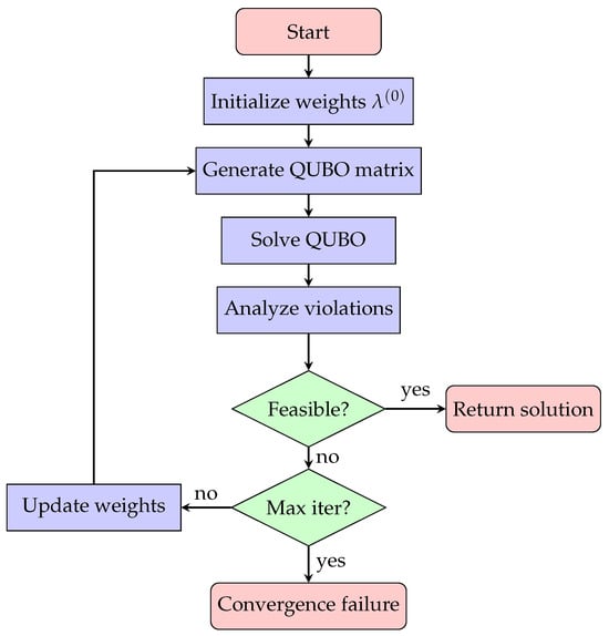
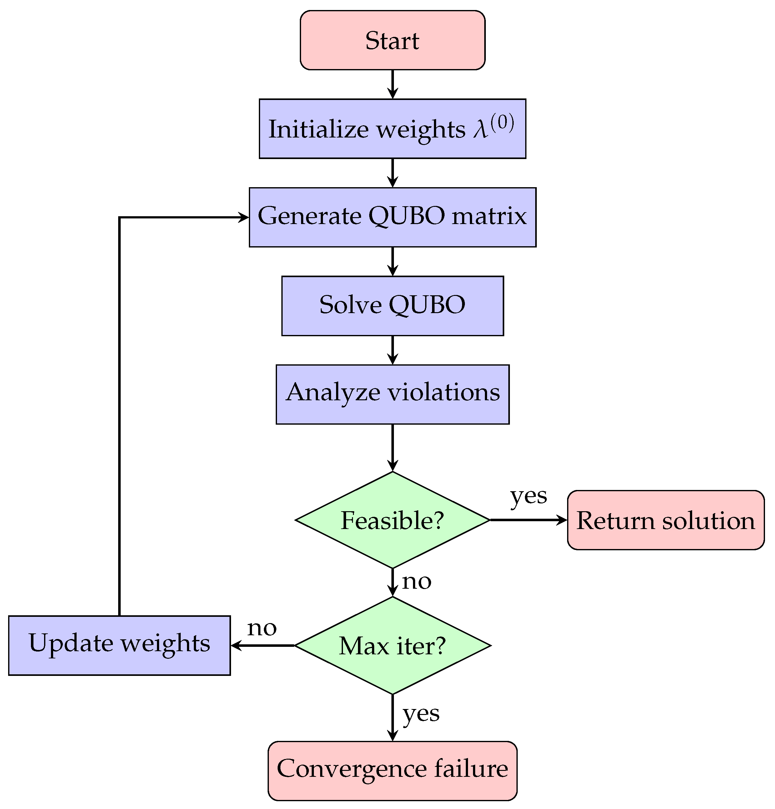
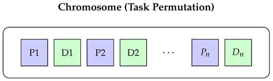
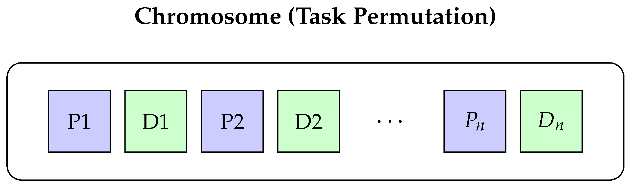
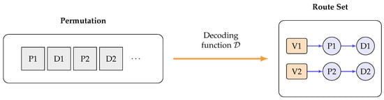
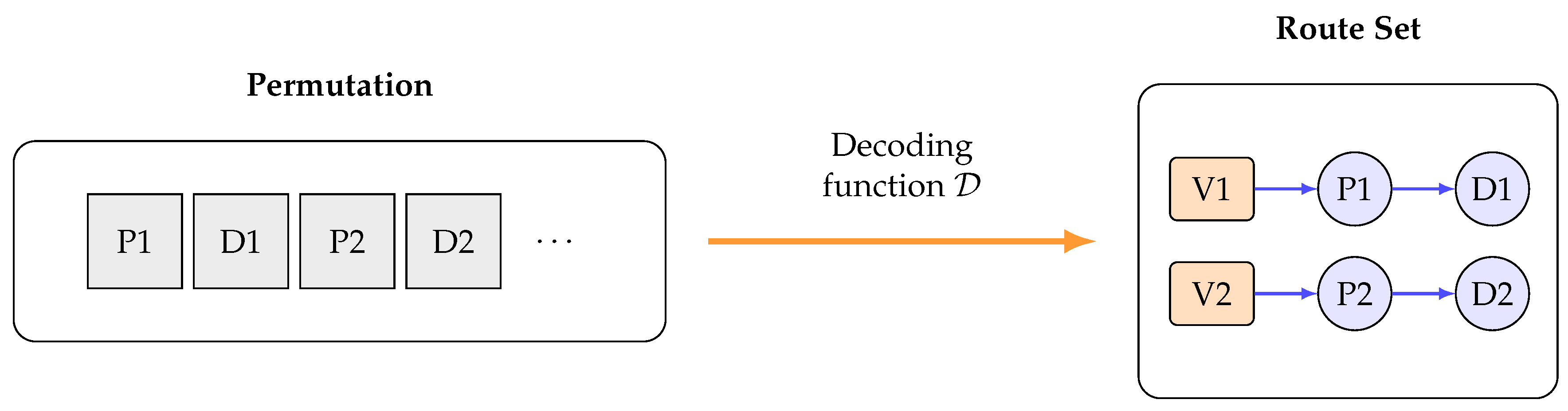
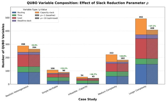
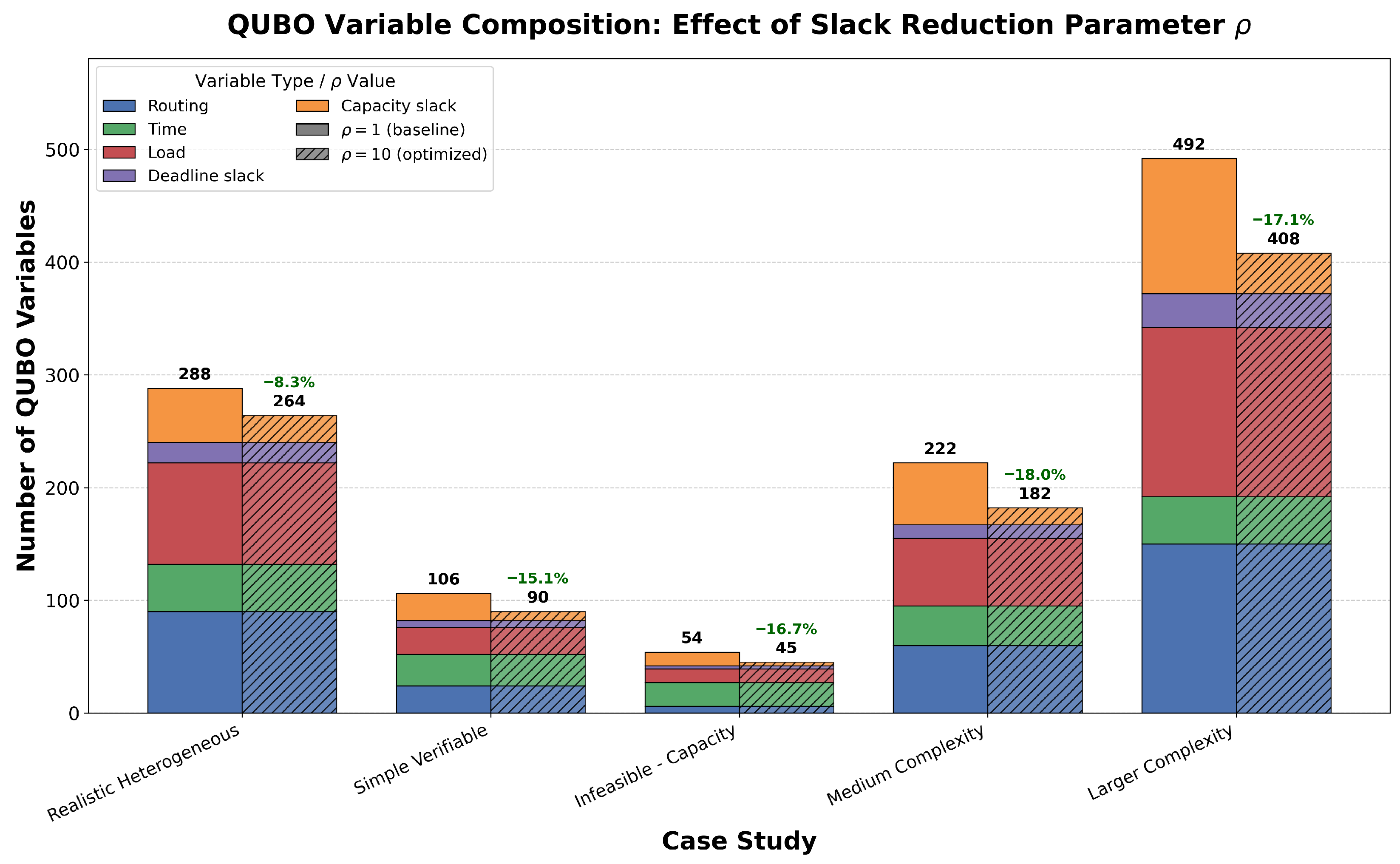
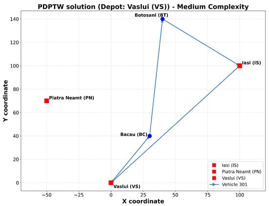
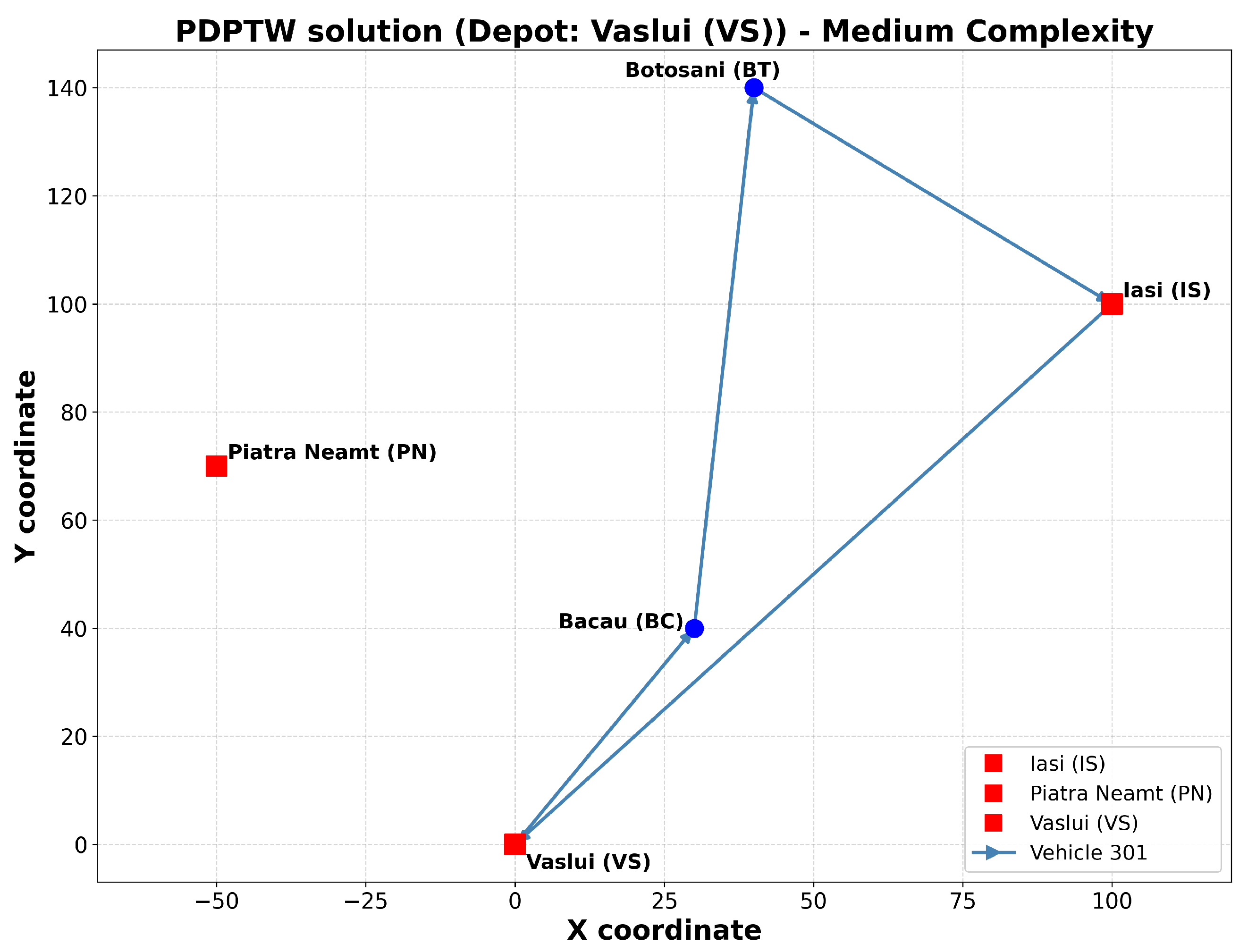
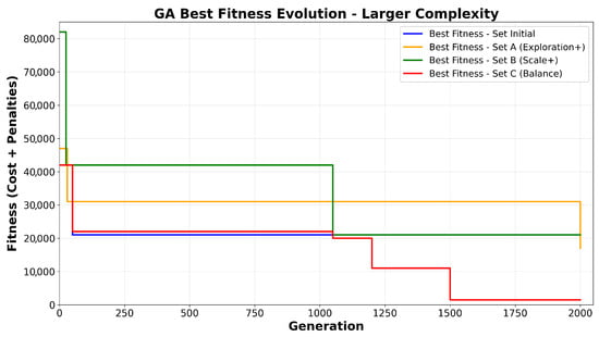
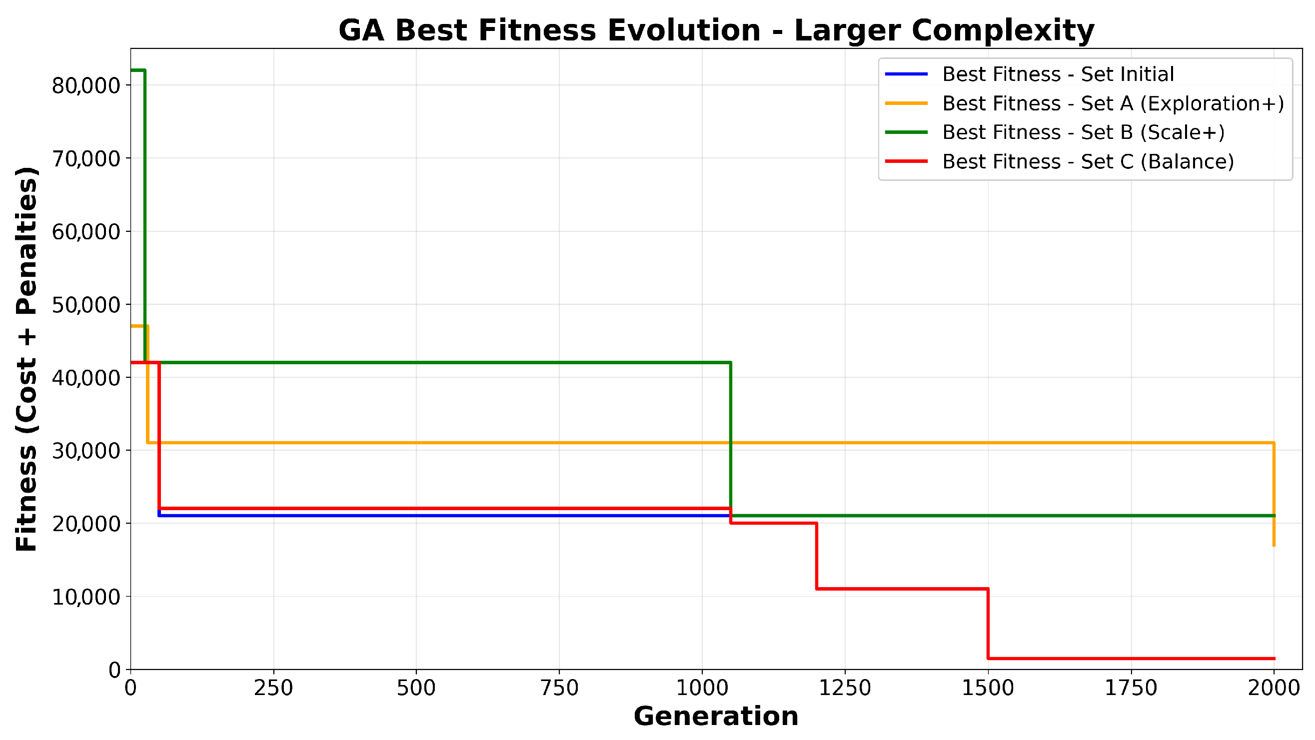
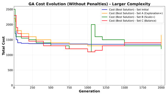
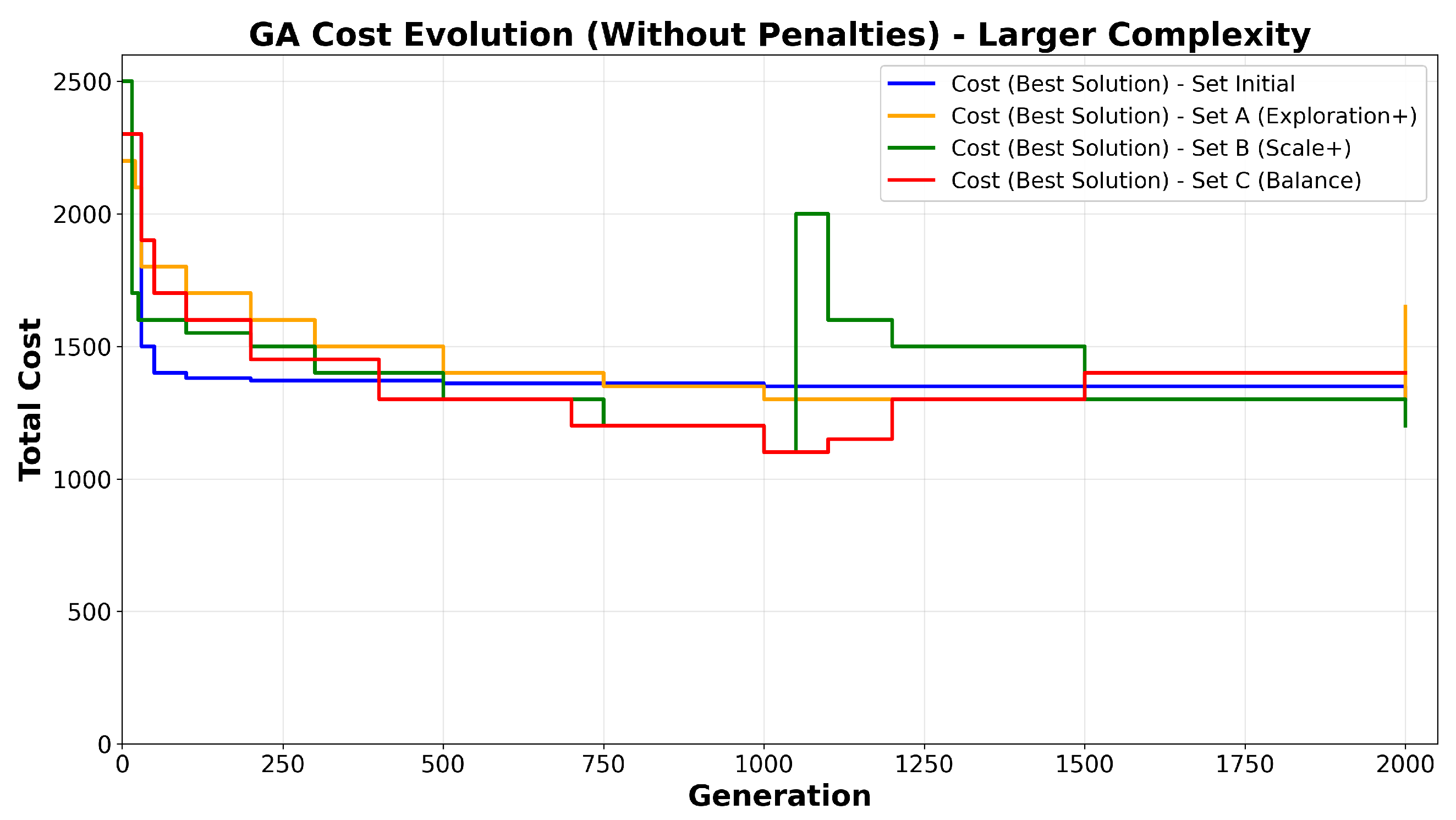
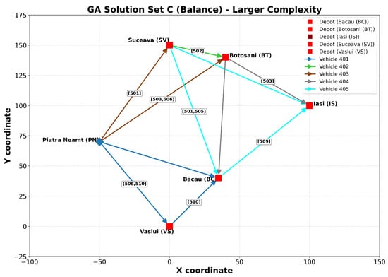
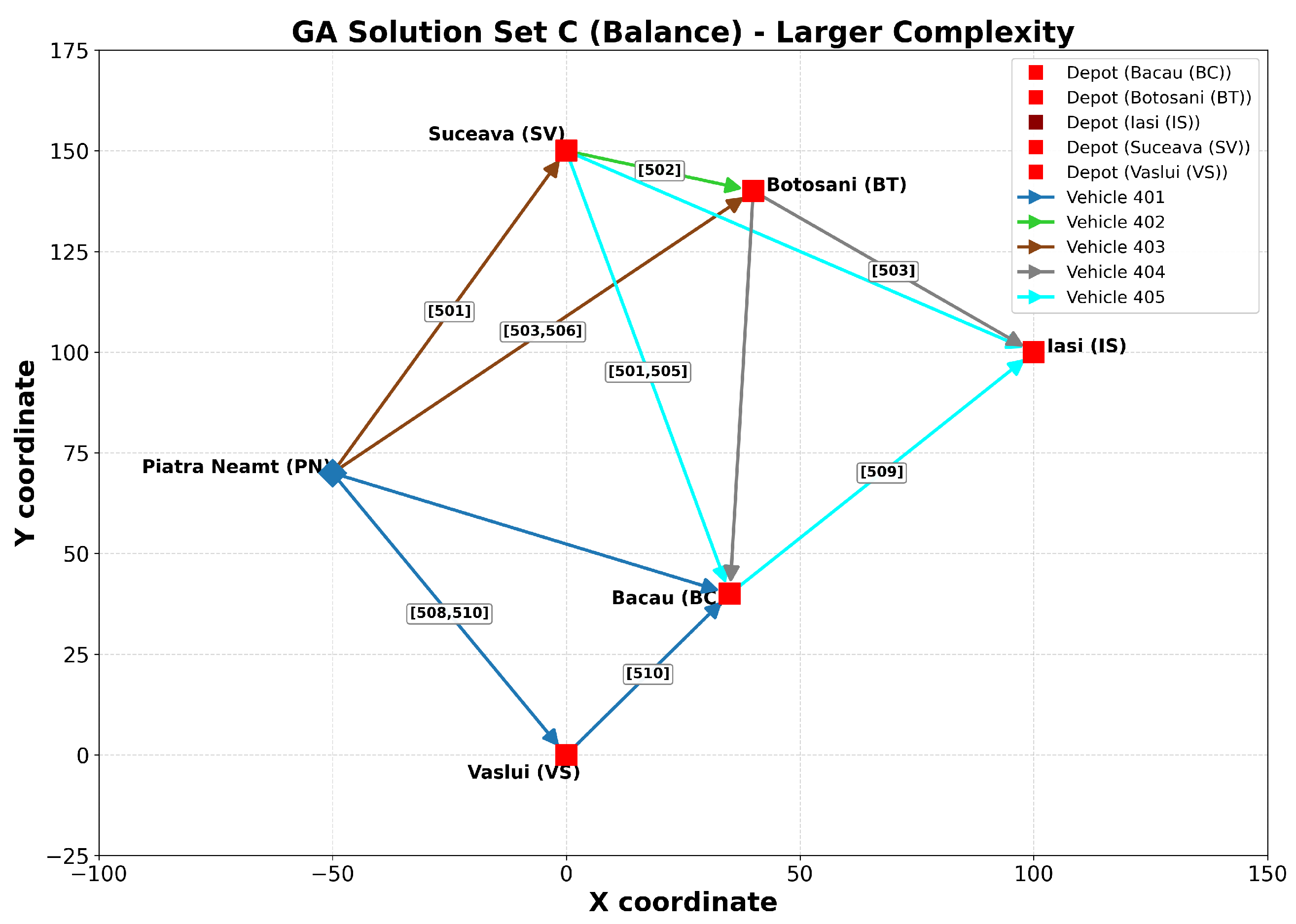
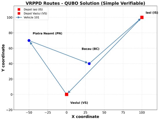
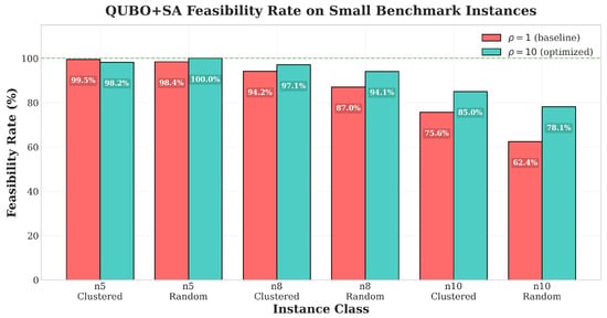
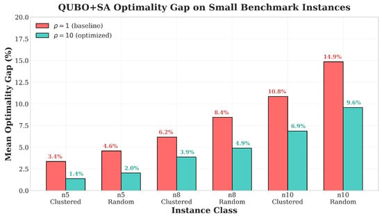
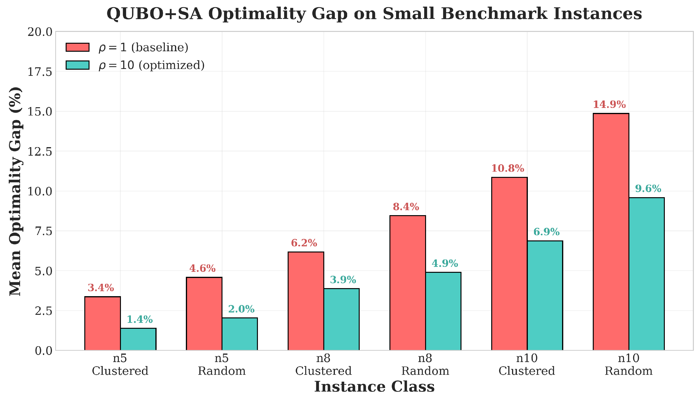
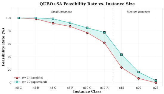
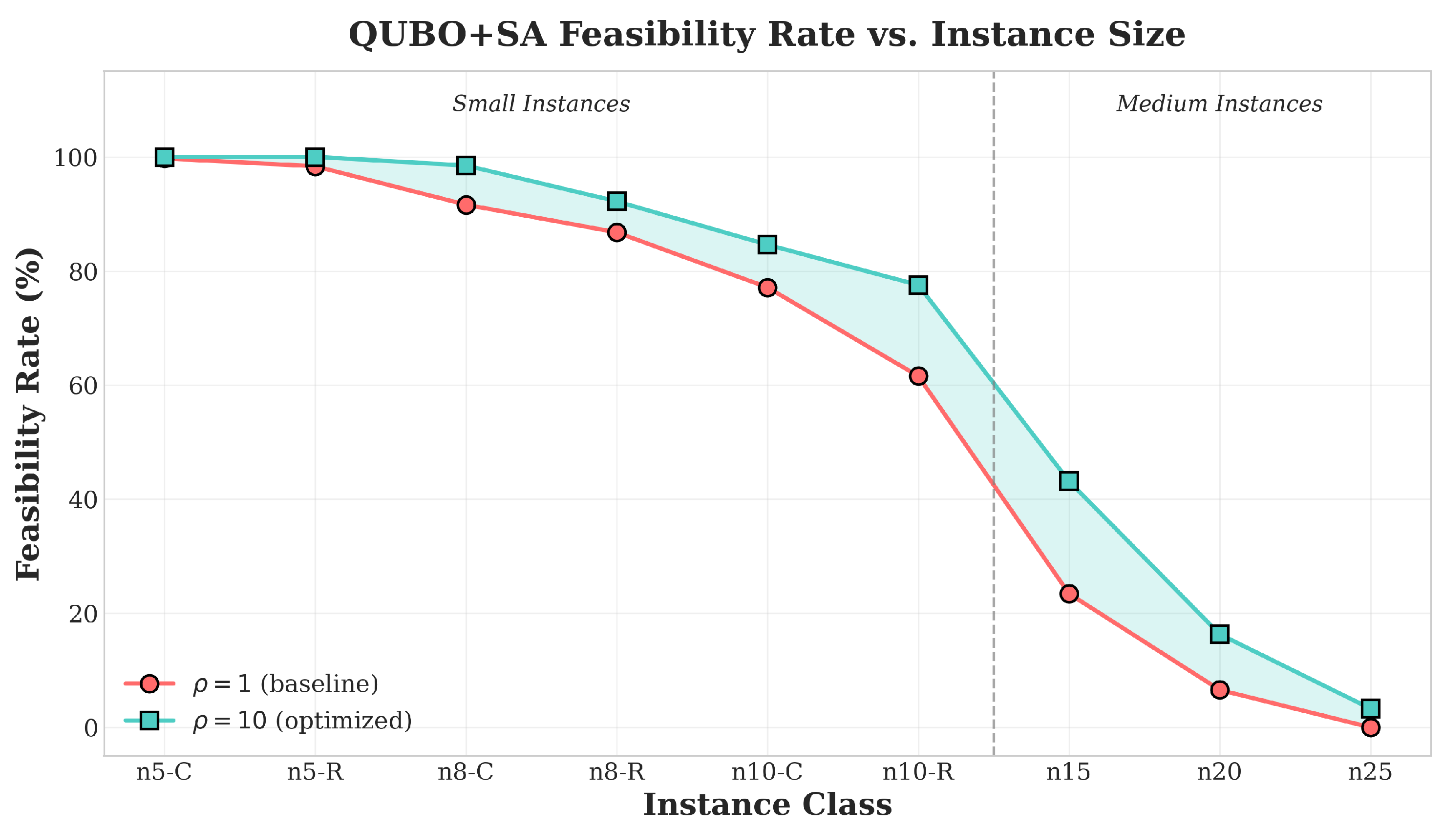
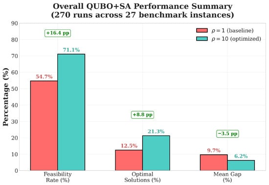
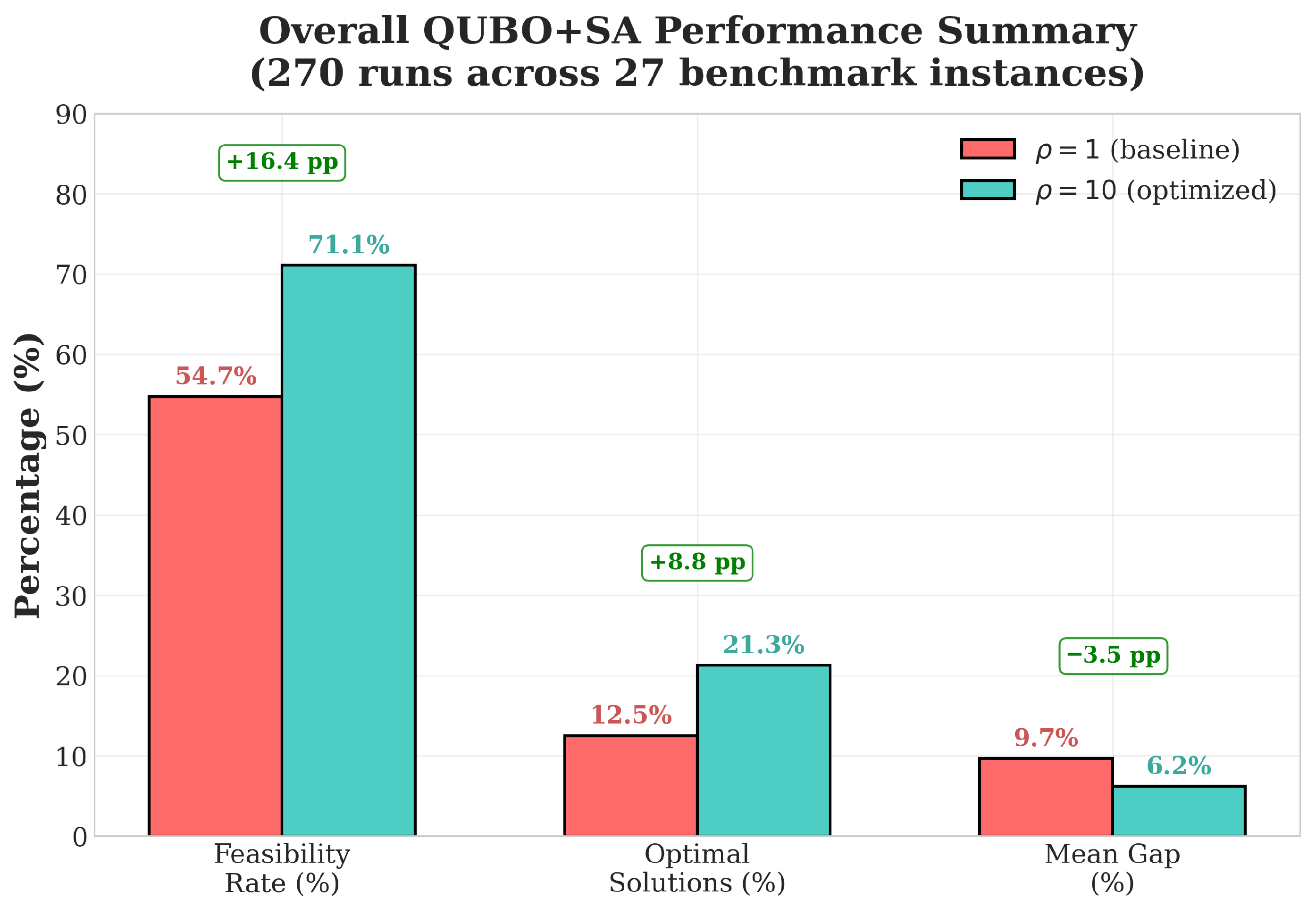
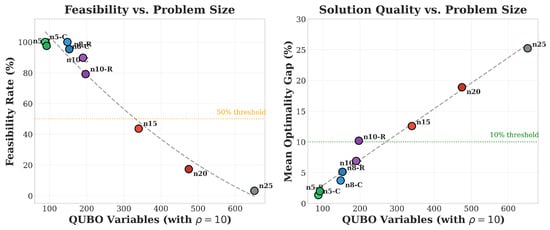
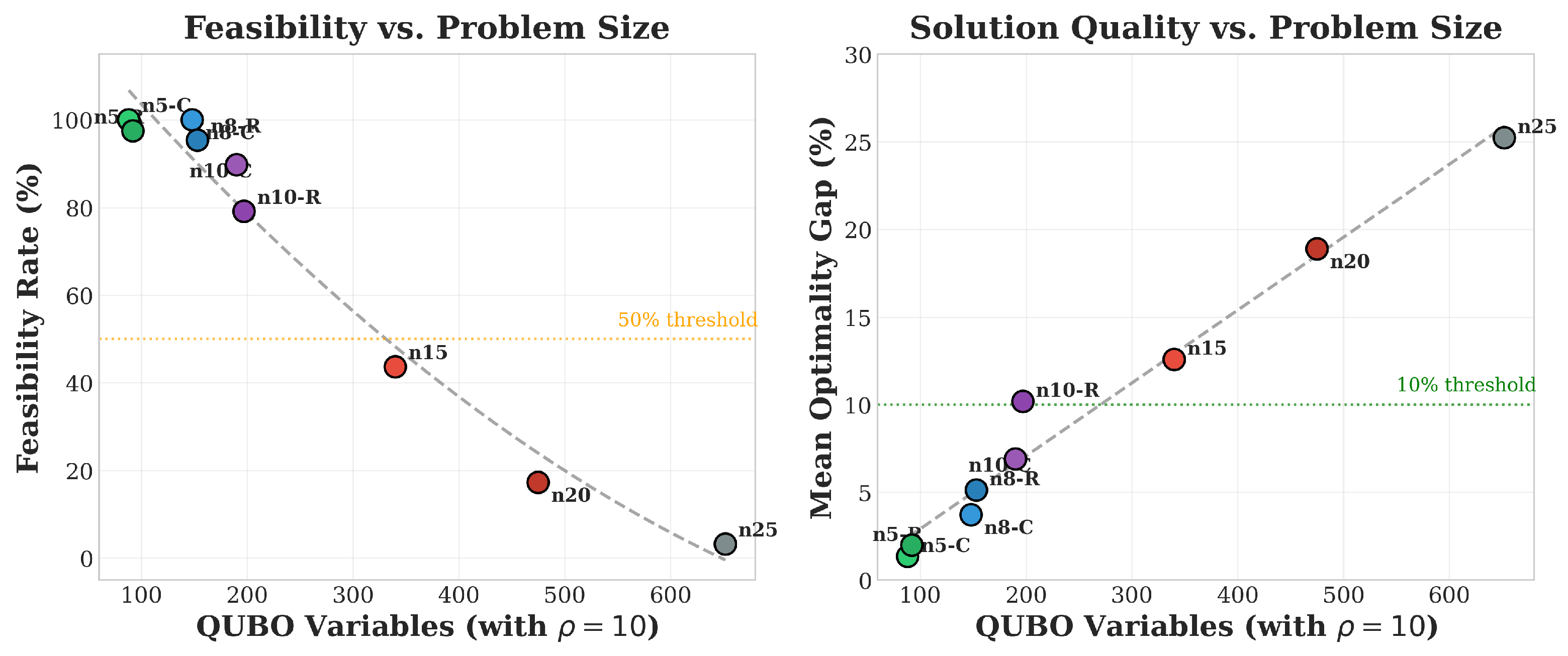
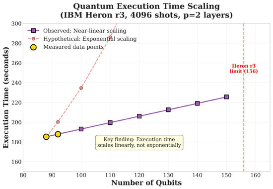
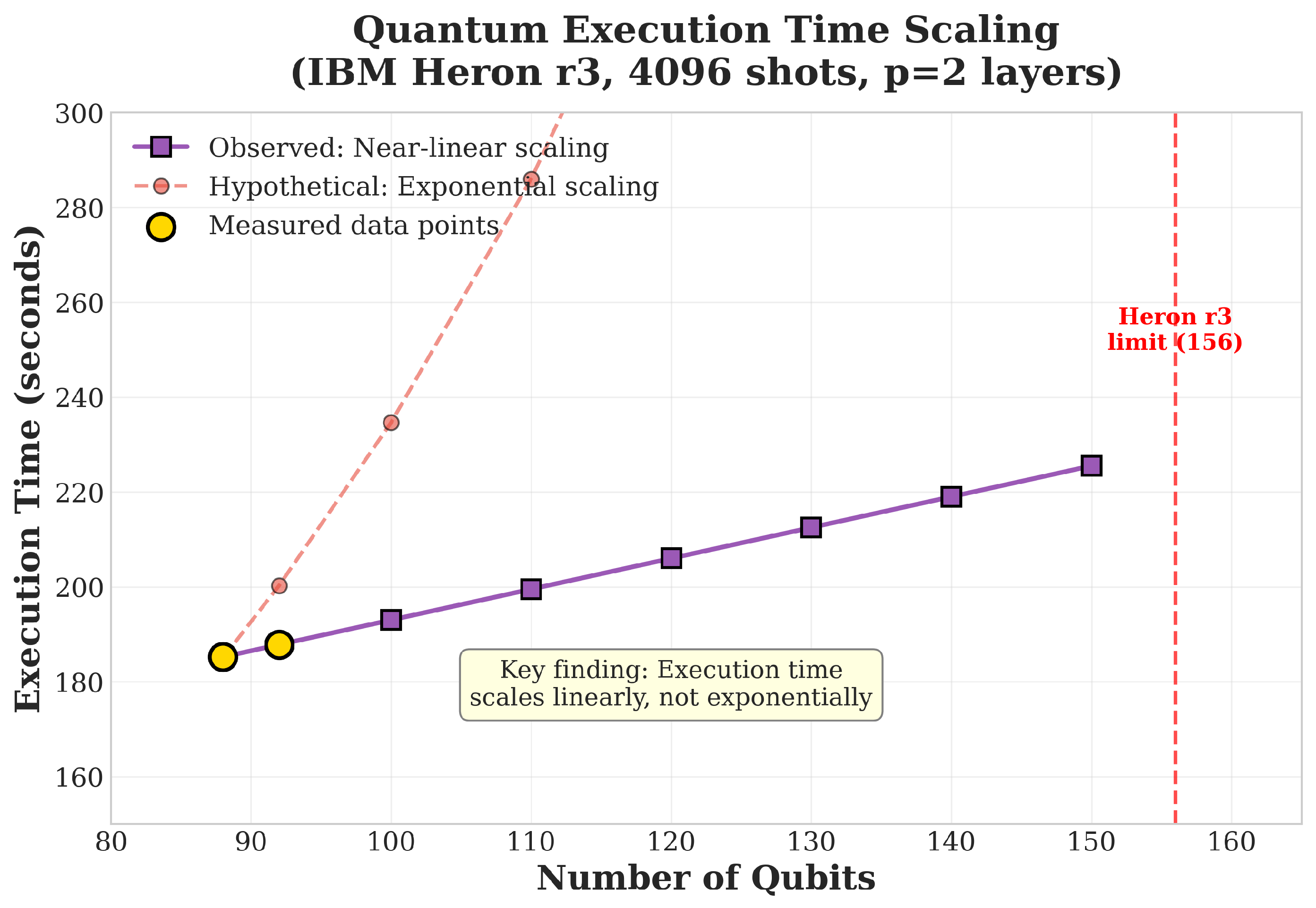
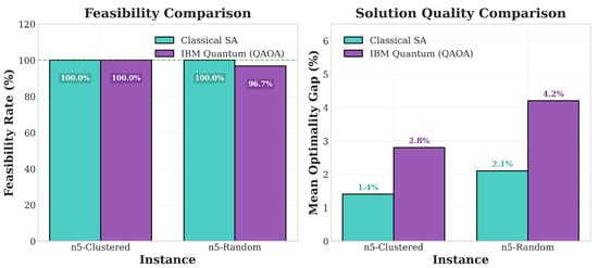
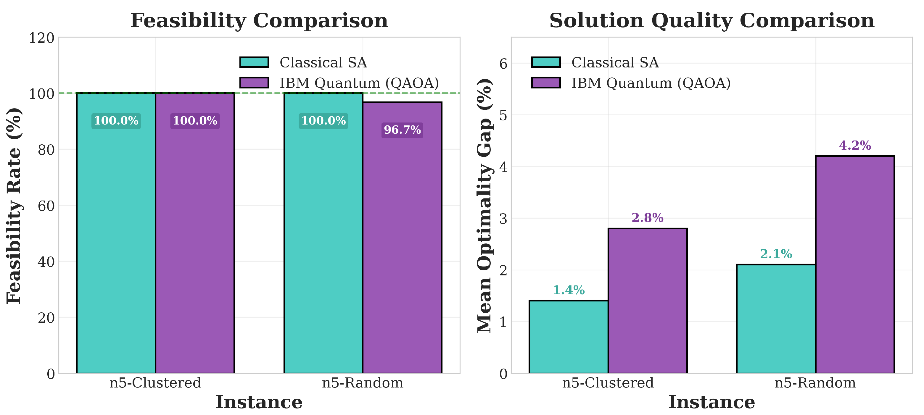

Disclaimer/Publisher’s Note: The statements, opinions and data contained in all publications are solely those of the individual author(s) and contributor(s) and not of MDPI and/or the editor(s). MDPI and/or the editor(s) disclaim responsibility for any injury to people or property resulting from any ideas, methods, instructions or products referred to in the content. |
© 2026 by the authors. Licensee MDPI, Basel, Switzerland. This article is an open access article distributed under the terms and conditions of the Creative Commons Attribution (CC BY) license.