Estimations of Production Capacity Based on Simulation Models: A Case Study of Furniture Manufacturing Systems

Abstract

This article presents the concept of building a discrete event simulation model of a production system in terms of statistical and probabilistic models, which is based on a fragment of a broader production process in the furniture industry. The purpose of the study was to evaluate the efficiency of a single-shift production process during the start-up phase and to determine the impact of implementing two- and three-shift systems. The discrete event simulation model was developed using actual production data collected during a single-shift operation. Scenarios were then designed to identify and quantify the necessary process adjustments required for the successful implementation of two- and three-shift systems. The authors demonstrated that simulation modeling of production processes based on probabilistic distributions provides information that is essential for effective capacity planning. The proposed percentile grids enabled clear visualization and precise assessment of production resource utilization in various shift configurations, facilitating decision-making regarding capacity expansion based on previously assumed data.

1. Introduction

Contemporary challenges and changes in global and local markets result in businesses being determined to constantly improve and adapt production process management methods to the current competitive environment [1,2]. Within the production management and enterprise development decision-making process [3], the management usually initiates activities aimed at implementing specific changes by identifying the entire system and then proceeds to formulate detailed objectives of the activities [4]. A natural approach in studying the actual production systems is conducting experiments [2] directly on a selected object [5], especially if it does not cause any undesirable effects (unplanned downtime, damage to machines and equipment, system breakdowns, etc.) [6,7]. However, such attempts are not always possible, as in many cases these kinds of activities may be impossible, difficult to implement, dangerous, expensive or time-consuming. In such situations, simulation models can provide support in the decision-making process by imitating the behavior of the actual system in experiments and then trying to evaluate, modify, re-analyze it and look for a better solution to the observed problem identified within the model [2,8,9]. Conducting research and analyses based on a simulation model is essentially loss-free and allows for the generation of many possible solutions, sometimes even very non-standard ones [8,9].

The purpose of this paper is to describe the approach to building a simulation model for the evaluation of a real manufacturing system on the example of the furniture industry, using statistical and probabilistic methods to analyze production capacity under variable conditions from the production capacity and resource utilization point of view.

2. Randomness Modeling and Simulation Based on Probability Distribution in Industrial Practice

The complexity and diversity of phenomena occurring in industry and the unpredictable nature of some events enhance the interest in process modeling and simulation [2,8,9,10]. Generally speaking, the purpose of the model is to imitate the behavior of a real system in order to analyze and evaluate it [6]. Many types of models for general production management can be found in the literature; however, to describe the actual production system using sets of symbols and relations, mathematical [6], statistical [11] and probabilistic [12,13] models are used. Computer-aided modeling of production systems and processes enables performing their computer simulations. The word simulation should be understood as an action that imitates or reproduces a phenomenon [6]. In the industrial practice, simulation is the reproduction of a selected real system through experimentation using a dedicated model. In this process, the role of the model is to represent the physical environment (usually in a visual, object-oriented way) and the surrounding logic that will determine the operations in the modeled environment [14]. The construction of a simulation model involves many preceding activities, including designing the general model and its detailed forms (e.g., using a computer software), defining the scope of the experiment, and preparing, processing, and analyzing data for the model. After the simulation is completed, additional activities are related to the analysis and interpretation of the results [8,15].

Also, there are many types of simulation models with different applications, and the choice of a specific one depends on the goals of the analysis and the behavior of the system itself. When addressing issues related to manufacturing systems, the following simulations deserve special attention: Monte Carlo, continuous processes, discrete events and agent-based [14]. In the case of discrete event simulation, the use of advanced simulation software with 3D functionality is widely used in implementing the guidelines of Industry 4.0 from the point of view of creating digital twins. Such activities are part of the digital transformation process, which effectively supports the efficiency and operational flexibility of enterprises, significantly improving the planning of changes [16]. These types of solutions include software such as: FlexSim, Tecnomatix Plant Simulation, Simio, AnyLogic, etc. [17,18,19,20,21].

Building a simulation model of an actual production system primarily supports the thinking process, as it stimulates the proper interpretation of the system operation, which often leads to the generation of new ideas and solutions. Effective simulation is achieved when the model is not oversaturated with excessive details of the system operation. Properly defining the purpose and level of detail of the simulation at the beginning of its creation allows for effective use of this tool for problem-solving. The key factor influencing the accuracy of the simulation result is the selection of the static time distribution of a given process.

The essence of controlling production processes characterized by the occurrence of parameter variability is the assessment of the so-called natural variability of characteristics. In the literature, it is usually referred to as the upper and lower control limits. Controlling such processes comprises reasoning based on the principles of probability theory and mathematical statistics [18,22].

A characteristic feature of phenomena occurring in production processes (including in furniture production) is their clear statistical nature [23,24]. Classical methods of assessing technological identification related to the processes of shaping materials included in the finished product, e.g., processing of furniture particleboards, are mainly assessed using statistical methods, and due to the very extensive mathematical apparatus, probabilistic models are rarely used [2]. In the literature devoted to modeling and simulation of production processes, probabilistic models based on the exponential, Weibull, normal, Gumbel, Ferecht, Reyleight, Gamma, and log-normal distributions [5,14,25,26,27,28,29] can be found. The presented distributions find their applications mostly outside the field of mechanical engineering [30,31]. A number of these distributions require the use of advanced numerical techniques and large sample sizes. In the case of assessing processes occurring in production engineering, it should be assumed from the outset that the probabilistic model used is able to provide information on the characteristics of changes occurring, for example, during the process of cutting a particleboard.

One of the main features of furniture processing is that the phenomena occurring in these processes can be classified as stochastic processes X(T,e), [5,25,32], i.e., as sets of random variables X_T(e) dependent on the parameter T, belonging to the set of real numbers $T\in (T_a,T_b)$. The $X(T,e)$ stochastic process can be defined as a set of random time functions assigned to elementary events - e, where the parameter - T generally denotes time (process cycle time) and frequency - f_c. One of the characteristic features of a stochastic process is the probability density function $f_1(x_1,T_1)$ for the process value x₁ and the time ${\mathrm{T}}_1$. With a fixed parameter $\mathrm{T}={\mathrm{T}}_0$, the stochastic process is a random variable $X({\mathrm{T}}_0,e)$. With a fixed elementary event $e=e_0$, the stochastic process $X(T,e_0)$ is a function of time $x\left(T\right)$ defined for $T\in (T_a,T_b)$ (called a realization of the stochastic process). The realization $x\left(T\right)$ of the stochastic process $X(T,e_0)$ is equivalent to the value $x$ that the random variable $X\left(e\right)$ takes with a fixed $e=e_0$. For any sequence of times, the probability density characteristics are more complex and for any sequence of times $T_1,\hspace{0.33em}{T}_2,\dots ,T_n$, a multidimensional random variable $X\left(T_1\right),\hspace{0.33em}X\left(T_2\right),\dots X\left(T_n\right)$ characterized by n-dimensional density $f_n(x_1,T_1;x_2,T_2;\dots x_n,T_n)$ should be considered. An ordered set of one-dimensional stochastic processes is called a multidimensional stochastic process.

In the case of furniture production, during the implementation of storage and manufacturing processes, the selection of appropriate statistical and probabilistic models is not clear. A significant group of manufactured furniture components operates in variable conditions that lead to disruptions in technological processes [2,10]. The occurrence of unforeseen failures and downtimes in the implementation of storage and processing of these components significantly complicates the calculation process of determining appropriate statistical or probabilistic models.

The starting point for determining the parameters which describe the duration of the processing of individual furniture components is the adoption of a statistically reliable probability distribution of the tested process based on experimental data. Statistical inference methods in the evaluation of the operation time can be based on knowing the form of the cumulative distribution function for the examined feature and are called parametric methods [33,34]. A distinction is made between graphical methods implemented using functional grids and analytical methods [35]. Parametric methods are more effective than non-parametric ones in the sense that a smaller random sample is required to obtain information about individual operation durations using parametric methods. When selecting the most appropriate mathematical model to determine experimental data, the physical aspects of the random events being studied should be taken into account, e.g., the type of material, the transport path, storage buffers, etc. Thus, using the probability distribution function, information about the individual parameters of the material movement variants is necessary.

A comparative analysis of selected studies is presented in Table 1.

Table 1. Comparative analysis of selected studies.

Authors	Review of Selected Literature
Ingaldi and Ulewicz, 2020 [1]	The publication concerns the concept of Industry 4.0, implemented mainly in large enterprises. The authors indicate the slower pace of implementation of new technologies in the SME sector and analyze the reasons for such disproportion.
Drobina, 2013 [5]	The article develops probabilistic models for assessing the fatigue strength of textile products. Probabilistic models were presented and compared with respect to strength tests.
Reussner et al., 2003 [6]	The authors developed a method for predicting the reliability of information technology systems, proposing an algorithm that allows estimating the reliability of the system architecture already at the design stage, using optimization methods.
Małopolski, 2012 [8]	The author presented methods for modeling and optimizing production processes in the Arena software. The presented topics were of a general nature and did not precisely describe the issues concerning extensive simulation related to real production conditions.
Łatuszyńska, 2015 [9]	The author presented a theoretical analysis of simulation methods in production management. Despite the lack of model validation, an important contribution of the work is the comparison of tools and the assessment of their usefulness in industry.
Kolny D. et al., 2023 [10]	The authors presented a methodology for building discrete simulation models based on actual production, using Arena software. The article disregards the probabilistic approach and is limited to simple simulations based on basic data.
Twardochleb, 2002 [11]	The author describes statistical modeling and optimization techniques in production processes. It presents the mathematical model of the system and the optimization of the parameters of a sample process. The theoretical nature of the work provides a good basis for designing experiments and research in industry.
Chomać-Pietrzecka, 2011 [12] Plucińska and Pluciński, 2000 [13] Drobina, 2013 [25] Weibull, 1939 [27], 1949 [28], 1951 [29] Li et al. [30]	The authors presented the application of probabilistic models in economic sciences [12] and materials engineering [25]. They described in detail the weakest link method and the survival analysis, referring to the works by Weibull [27,28,29]. The presented theory was used to implement the developed models in the FlexSim environment.
Beaverstock et al., 2019 [14]	The authors present a simulation research methodology that enables designing, testing and optimizing production or logistics processes in a virtual environment.
Ciszak, 2007 [15]	The author presents a method of computer modeling and simulation of technological processes used in the machinery industry. This is a review article, but it serves as an excellent aid in learning how to create simulation models.
Kritzinger et al., 2018 [16]	In the article, the authors have thoroughly organized and systematized the concepts related to production virtualization. They defined, described and classified the terminology related to the digital twin concept.
Florescu and Barabas, 2020 [17]	The authors used a software that enables mapping of the system structure and assigning key technical and cost indicators to the system. By testing various scenarios in a virtual environment, solutions were identified that maximize the efficiency of manufacturing and transport processes.
Lewicki et al., 2024 [18]	The paper focused on the optimization of the production process in the automotive industry, with particular emphasis on employee workload and identification of bottlenecks. Failure rate issues were presented and the developed models were assessed. Despite outlining the probabilistic aspects, the authors did not include data on simulation replication and did not go beyond a general description of the operation of the models.
Mokshin et al., 2019 [19] Kikolski, 2016 [20] Zaayman and Innamoratov, 2017 [21] Karkula, 2013 [36]	The publications provide an overview of the practical application of leading simulation environments in solving operational problems in industry and logistics, which presents a wide spectrum of available technological solutions.
Alot, 2014 [22]	The author presented a proposal for the use of statistical tools to control production processes and the use of the tools for the evaluation of the control of logistics processes. The work is of a general nature and provides a basis for the development of simulation models, with particular emphasis on the validation of the obtained statistics.
Czabak-Górska et al., 2015 [23]	The publication presents a statistical system which enables objective classification of measurement results as outliers or standard values, which eliminates subjectivity in data selection. As part of a case study based on real production parameters, the authors presented a practical algorithm for using these tests to identify gross errors.
Czader and Szpoczek, 2015 [24]	The authors presented the use of statistical tools to assess the quality of manufactured components. Their considerations focused on the use of the SPC method in a production environment.
StatSoft, 2025 [26] Stanisz, 2006 [33,34]	The books present professional statistical analysis for industrial and scientific applications. This literature supports researchers in conducting analyses in the Statistica environment.
Afolabi et al., 2025 [31]	The paper discusses methods for optimizing stochastic objects and presents probabilistic models that were used to map production processes and identify bottlenecks. The results of the analysis enabled identifying places that determine the dynamics of the process.
Mańczak, 1979 [32] Benjamin and Cornell, 1977 [35]	The publications discuss in detail the identification of mathematical models and the theory of experiment design, as well as the use of statistical methods to analyze processes in industrial conditions.

3. Building a Simulation Model in the FlexSim Environment Using a Furniture Manufacturing Company as an Example

When creating a model of the studied manufacturing system, it is necessary to collect basic information and input data regarding the specific nature of its operation. In the initial phase, a model is developed at an appropriate level of detail while not complicating the entire system of the model [15]. The next part of the article will present the process of building a model for a particleboard cutting system in line with a production order, which is referred to as cut layout in the furniture industry. The design of the essence of the analyzed manufacturing system model was limited to the moment of the buffer storage of cut particleboard elements (two possibilities can take place here, i.e., the process of packaging the elements for assembly or further processing for the finished assembly, which will not be analyzed in this article). The FlexSim software version 23.2.2 (Autodesk Inc., San Francisco, CA, USA) was used to build the simulation model, and its detailed parameterization was based on statistical analyses performed using Statistica 7.1 environment (StatSoft Polska Sp. z o.o., Kraków, Poland). The studies were carried out in actual production conditions on a newly built production line.

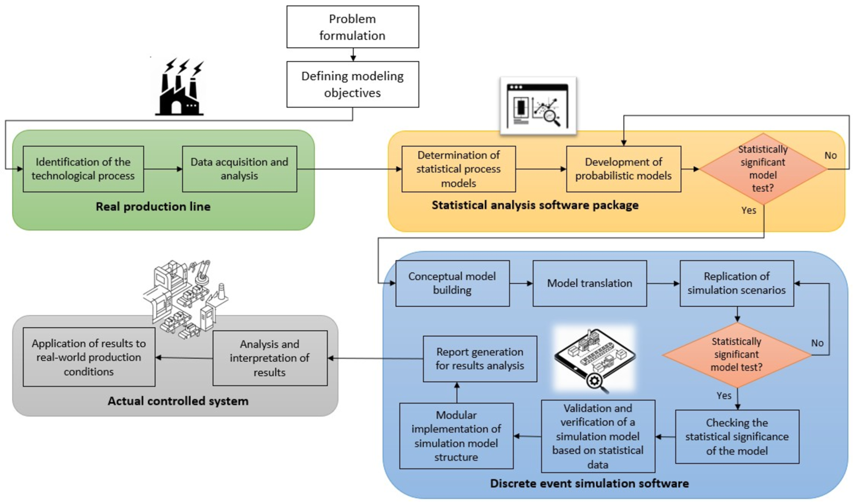
The algorithm of the modeling procedure is shown in Figure 1.

Figure 1. Conceptual model of the simulation model architecture (own study).

Problem formulation in the simulation modeling process begins with identifying the system and setting the modeling objectives. This process involves defining the boundaries between the system being studied and its environment and isolating the significant interactions that connect the items to actual production conditions. It is crucial to define parameters, variables, constant coefficients, as well as functional dependencies and probability distributions. Building a conceptual model consists of the quantitative and qualitative representation of the static and dynamic infrastructure of the studied object. It is important to select the level of detail of the model that is appropriate to the goal. In the initial phase, the simulation model is built based on simplifications. Then, the desired complexity is selected—significant level of detail results in a model that reflects the actual production system better. However, it should be noted that introducing details that may prove to be irrelevant makes the implementation, verification and validation of the model more difficult. The correct selection of the level of detail allows for avoiding having to rebuild the entire model in later stages. The collection and pre-processing of numerical data are the basis of statistical analysis and feeding the model with input data. The quality of the simulation model is influenced by the appropriate selection of data, the researcher’s experience and empirically obtained information about the problem. In industrial practice, statistical and qualitative tools are used for this purpose. The input data is used to determine the theoretical and empirical probability distributions according to which pseudo-random numbers are generated. The use of raw (historical) data only allows for the simulation of the past behavior of an object. This simplifies the verification but limits the predictive potential of the simulation. Model translation involves its implementation in a selected programming language or simulation package. An extremely important stage is verification and validation, i.e., checking the correctness of the model against its real counterpart. The first step in validation is usually comparing the simulation results with the performance of the actual system for identical input data. Design of experiments (including the number of replications) involves defining research scenarios and input parameter values. A proper design of experiment should provide maximum information with minimum computational effort. The process ends with conclusions and the generation of reports and documentation [36].

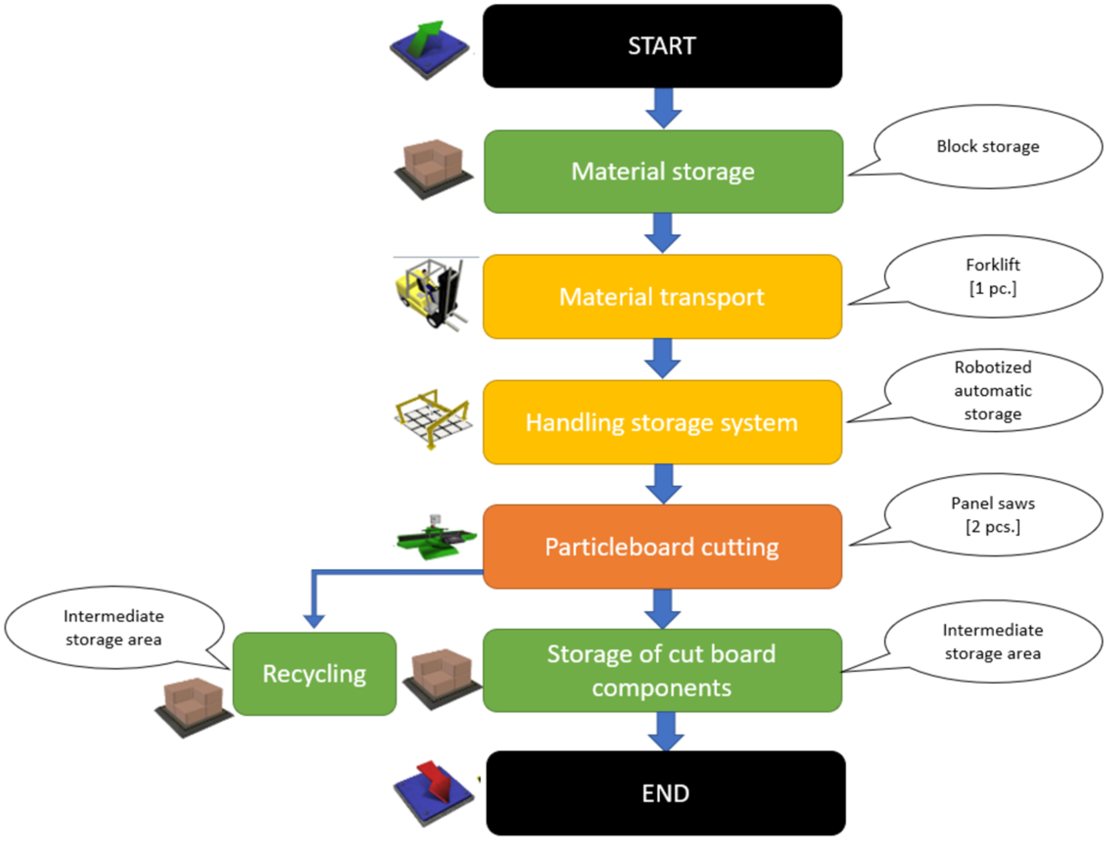
The initial phase of building a simulation model of the analyzed furniture manufacturing system involves technological identification of the particleboard cutting process. As a result of this identification, the phenomena occurring in the discussed production process were characterized. Process sheets, available machine documentation, as well as historical data on the times of handling and processing operations recorded by the machines used in the production process, were used for this purpose. The sequence of consecutive storage, handling and machining processes for the implementation of the discussed manufacturing system is presented in Figure 2.

Figure 2. The process flow of particleboard cutting (own study).

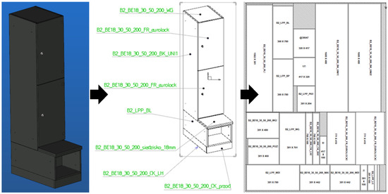
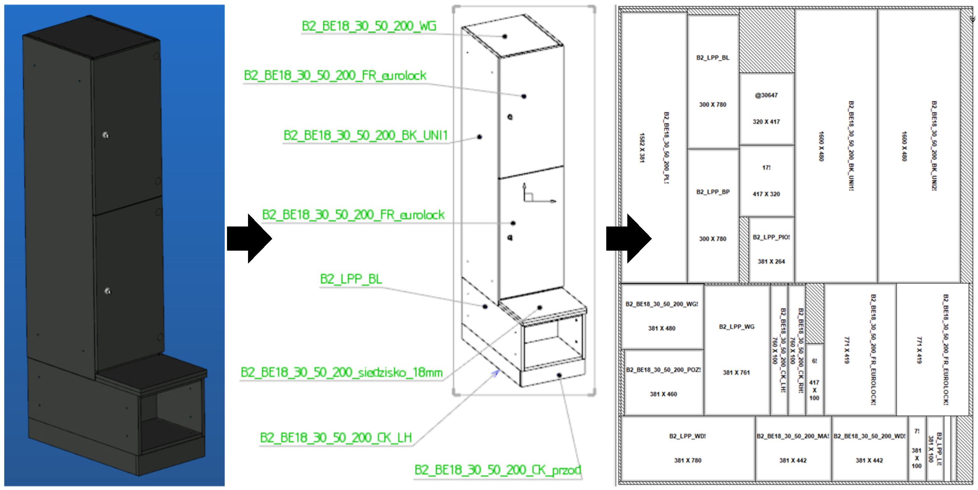
The detailed, quantitative flow of material at individual stages of the manufacturing process is often the result of many factors, including mainly the variant of the finished product being manufactured. In the discussed case, it is a cabinet with a seat with the following dimensions: a length of 750 mm, a width of 423 mm and a height of 2000 mm, custom-ordered by a client (Figure 3). Specialized software, such as Cut Rite, is used in industrial conditions of the analyzed enterprises [37] to optimize the cut layout planning process to ensure the most effective use of the chipboard surface for the given dimensions of the cabinet with a seat. The data obtained from cut layout were used only to illustrate the specific production characteristics.

Figure 3. Assembly drawing of the cabinet with the codification of individual components with cut layout of the particleboard [37].

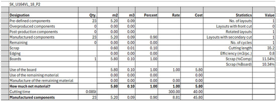
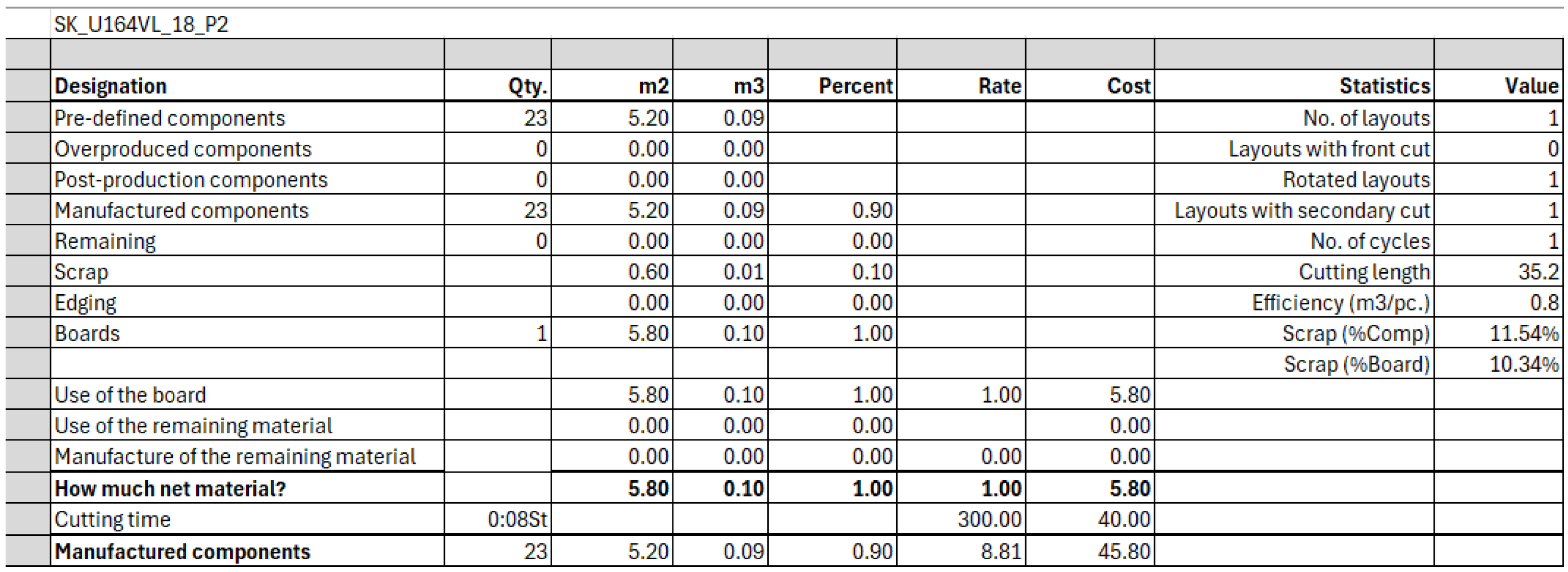
Selecting the chipboard cut layout that is optimal for a given furniture design has a significant impact on the efficiency of the production process in terms of material use. For the simulation model in the discussed manufacturing process, the key parameters resulting from the cut layout are the particleboard parts constituting the elements of the finished product and the recycled scrap, respectively. This information was also obtained from Cut Rite software V12.00.5 (Figure 4). In the case in question, 90% of the surface of the cut particleboard constitutes elements of the finished product (cabinet), while the remaining 10% is scrap collected in an appropriate container and then recycled. It is also worth noting that the type of cut layout (number and length of cuts) affects the duration of the operation.

Figure 4. Summary of material use efficiency resulting from the cut layout [37].

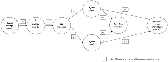
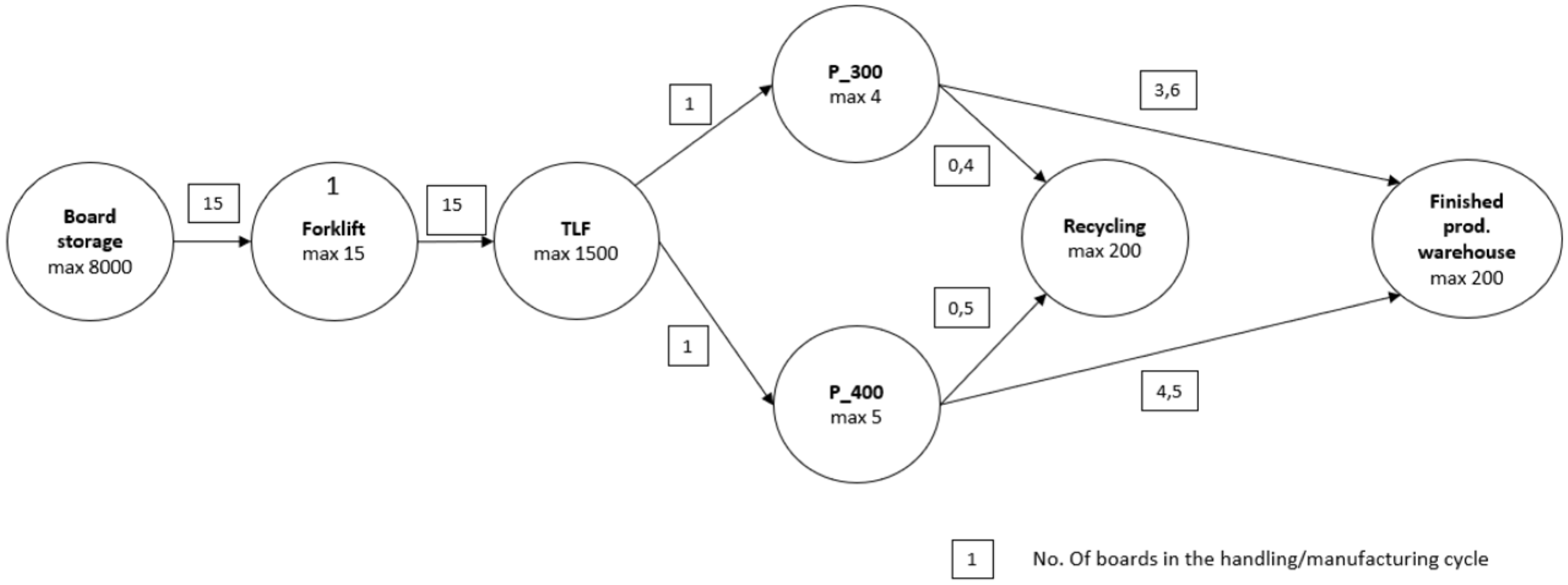
The implementation of the discussed manufacturing process of cutting particleboards proceeds with a variable quantity of material between subsequent stations. Important parameters include: the capacity of the station (buffer), the number of boards picked in one handling cycle, the number of boards picked in one processing cycle and the scrap constituting a specific part of the particleboard. The graph of material flow between stations (expressed in the number of boards) together with the buffer values are presented in Figure 5.

Figure 5. Material flow graph (particleboard sheets) for item P1 (own study).

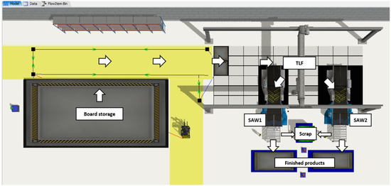
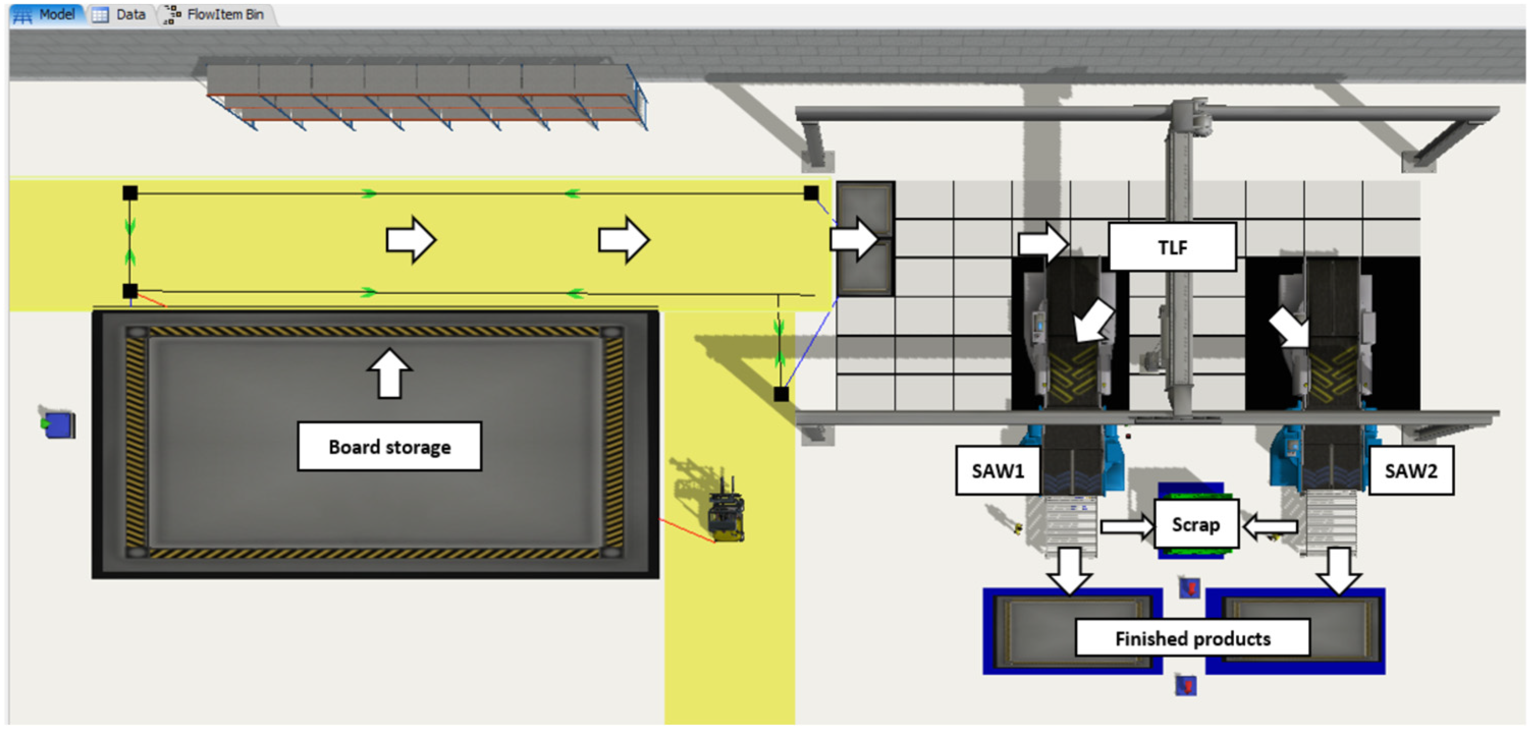
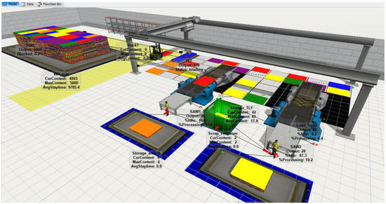
Analyzing the data in Figure 5, it can be concluded that the material flow and throughput between the stations vary. In the analyzed manufacturing system, it was assumed that the board storage could hold 8000 pieces of particleboards. The forklift picks 15 pieces of particleboard from the storage in one transport cycle, transporting them to the special loading bays of the TLF handling robot storage system. The TLF storage system capacity is 1500 particleboards. The TLF station handles one particleboard in one handling cycle (loading or unloading). Panel saws (SAW1 and SAW2) usually cut boards in one cycle (four and five pieces in a package for one station, respectively) according to the planned cut layout. As part of this operation, it was identified (Table 1) that 90% of the surface of a given board constitutes the base for the construction of the finished product, and the remaining 10% is production scrap that is recycled. All data entered into the model comes directly from the company’s operator panels, their registers and related programs. The visualization of the manufacturing system model in the FlexSim environment is presented in Figure 6.

Figure 6. Simulation model of a fragment of the furniture manufacture system in the FlexSim environment (own study).

The above simulation model constitutes the basis for further work aimed at the analysis of the production capacity of the studied manufacturing system. The model reflects the logic of its operation, the relationships between stations, buffer and storage capacities, and the appropriate sequence of performing the manufacturing tasks. The next stage of the analysis is adopting appropriate durations of operations at individual stations based on the numerical data of the machines and the statistical and probabilistic models developed based on them.

The essence of controlling production processes characterized by the occurrence of parameter variability is the assessment of the so-called natural variability of characteristics. In the literature, it is usually referred to as the upper and lower control limits. Controlling such processes involves reasoning based on the principles of probability theory and mathematical statistics [22].

A characteristic feature of phenomena occurring in production processes (including in furniture production) is their clear statistical nature [23,24]. As mentioned, classical methods of technological identification during the processing of furniture components are mainly assessed using statistical methods, and due to the very extensive mathematical apparatus, probabilistic models are rarely used [2]. In the literature devoted to modeling and simulation of production processes, probabilistic models based on the exponential, Weibull, normal, Gumbel, Ferecht, Reyleight, Gamma, and log-normal distributions [14] can be found. The presented distributions find their applications mostly outside the field of mechanical engineering. A number of these distributions require the use of advanced numerical techniques and large sample sizes. In the case of assessing processes occurring in production engineering, it should be assumed from the outset that the probabilistic model used is able to provide information on the characteristics of changes occurring, for example, during the process of cutting a particle board.

4. Selection of a Probabilistic Model for Assessing the Duration of Selected Manufacturing Processes in the Distribution

When modeling simulations of an actual manufacturing system, probability distributions are important because they allow to account for the occurrence of variability and randomness in manufacturing processes. In practice, the selection of the probability distribution often results from a thorough analysis of the relevant historical data collected from the studied manufacturing system. There are two approaches to analyzing historical data [18,36]:

• Parametric—estimating the parameters of the assumed probability density function based on historical data, and then comparing different functions to select the one with the best fit;
• Non-parametric—based on historical data without any assumptions as to how to fit the function to it.

Appropriate fitting of the probability distribution requires an appropriate size of the historical data set (according to A. Law, a proper sample consists of 100–200 measurements). Another important aspect when evaluating data is the identification of outliers—using the a posteriori selection method [5,18,36]. Their value differs significantly from the values of the other elements (e.g., due to an error or mistake) and it is good practice to remove these data to avoid incorrect assignment to a family of distributions due to the skewness that they cause.

The selection of appropriate statistical and probabilistic models for the simulation of furniture production during the particleboard cutting process using an automatic board feeding storage system is not obvious. A significant group of furniture products operates in variable conditions that lead to various disruptions in technological processes, which may result in economic losses. The occurrence of breakdowns or short unplanned downtimes of handling devices in furniture products significantly complicates the calculation process of determining appropriate statistical or probabilistic models, without which the simulation results may differ from the probable actual ones.

In this paper, a graphical method [5] was used to obtain an assessment of the fit of the probabilistic model. Using this method in mechanical engineering is justified by the possibility of quickly determining the values of distribution parameters. The verification of the correctness of the manufacturing process description against a given probability distribution was based on the so-called probability grid, in which the abscissa axis represents the value of the operation duration, and the ordinate axis specifies the probability P. The probability grid constructed in this way presents a complete graph of the operation duration in a probabilistic approach. The probability (P) of the duration of the operation at the manufacturing stations was determined according to the formula which takes into account the probability of the operation duration equal to 50% [5]:

$$P={\displaystyle \frac{\mathrm{i}-0.5}{\mathrm{n}}}\ast 100\%$$

where

• i—ordinal number of the sample,
• n—number of acquired operation duration samples.

The almost linear arrangement of points (individual duration trials of the operation) may indicate that the data distribution is adequate. In the conducted study, it was assumed that the points corresponding to the actual operating conditions of the machines and the manufacturing process within the error range of α = 0.05 caused by variability would form a straight line.

The study proposed to assess the properties of technological processes using selected distributions, such as [5,18,27,29,33,34]:

• Normal distribution;
• Log-normal distribution;
• Weibull distribution;
• Triangular distribution;
• Rayleigh distribution;
• Johnson’s distribution.

In order to verify the nature of the distribution, the so-called probability grid was used. The value of the operation duration is represented on the abscissa axis, and the probability P is represented on the ordinate axis. The least squares method can be used to estimate the parameters of probabilistic models; however, its disadvantage of excessive sensitivity to “outlier” observations should be taken into account. The estimation results may be distorted in these cases. Therefore, the paper uses the maximum likelihood method, which is based on the likelihood function. It can be applied to models including an additive random component with an assumed distribution type. Numerical techniques were used to develop the distributions. A detailed numerical analysis of the duration of operations at the analyzed stations and the verification of hypotheses were carried out using Statistica 7.1 statistical analysis software. A confidence level of 95% was assumed and the Anderson–Darling test [25] proposed in the software, which employs the mean square distance, was used. It is the weighted average of the squares of the distance between the empirical and model cumulative distribution functions.

The comparison of experimental data with the assumed statistical model developed for selected probability distributions was performed using a graphical method. It was assumed that the points corresponding to this data (within the error limits caused by sampling variability) would form a straight line. In order to determine specific distributions, a functional grid corresponding to a given type of determined distribution was used (the Weibull distribution and the normal distribution in the analyzed case). In practice, functional probability grids differ only in the scale necessary to “straighten” the graph representing the assumed model. In both cases, a functional grid was used, assuming that if the model of this distribution is correct, the curve drawn on the functional grid is expected to form a straight line. In practice, the 50% percentile line largely reflects the average values obtained from actual measurements.

5. Development of Probabilistic Models for Estimating the Duration of Technological Operations

The tests were conducted in real manufacturing conditions during the start-up phase of a furniture production line. Time data were obtained for a 6-month period during which the company operated in a single-shift system from 6:00 a.m. to 2:00 p.m. Actual numerical data on the duration of technological operations from the machines were used to develop probabilistic models for the conducted research. The time of individual operations has a significant impact on the completion of a furniture production order. For each operation, a sample of 100 cycle time measurements and component production volume data from a period of 100 consecutive days was analyzed.

As part of the experiment, the decision was made to assess production capacity also in the context of possible 2- and 3-shift system of work. For this purpose, it was decided to carry out a simulation with reference to time series (historical numerical data obtained directly from the machine operator panels) [34], which constitute the material and data used as input for the simulation. It was also decided that the capacity or predictability of production is to be assessed using probabilistic models. Based on the percentile grids, it was assumed that the level of 50% would correspond to the typical operation of the technological line in the start-up phase, which in fact corresponds to the average values obtained from the experiment in actual conditions. Additionally, the 25% and 90% levels were statistically analyzed to estimate production capacity under two scenarios. The level of 25% would characterize the optimistic scenario, i.e., the processes completed in a shorter time as compared to the level of 50%, and the level of 90% would characterize the pessimistic scenario, i.e., the processes completed in a longer time (e.g., due to unforeseen downtimes). Numerous experimental studies show that random industrial disturbances can in most cases be described by a normal probability distribution. In the case of other probability distributions, the least squares sum principle can also be used to determine the regression coefficients, but with the caveat that the resulting estimates may be less effective.

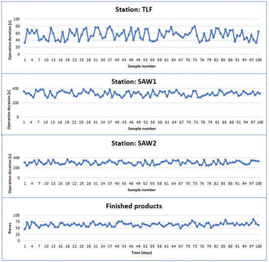
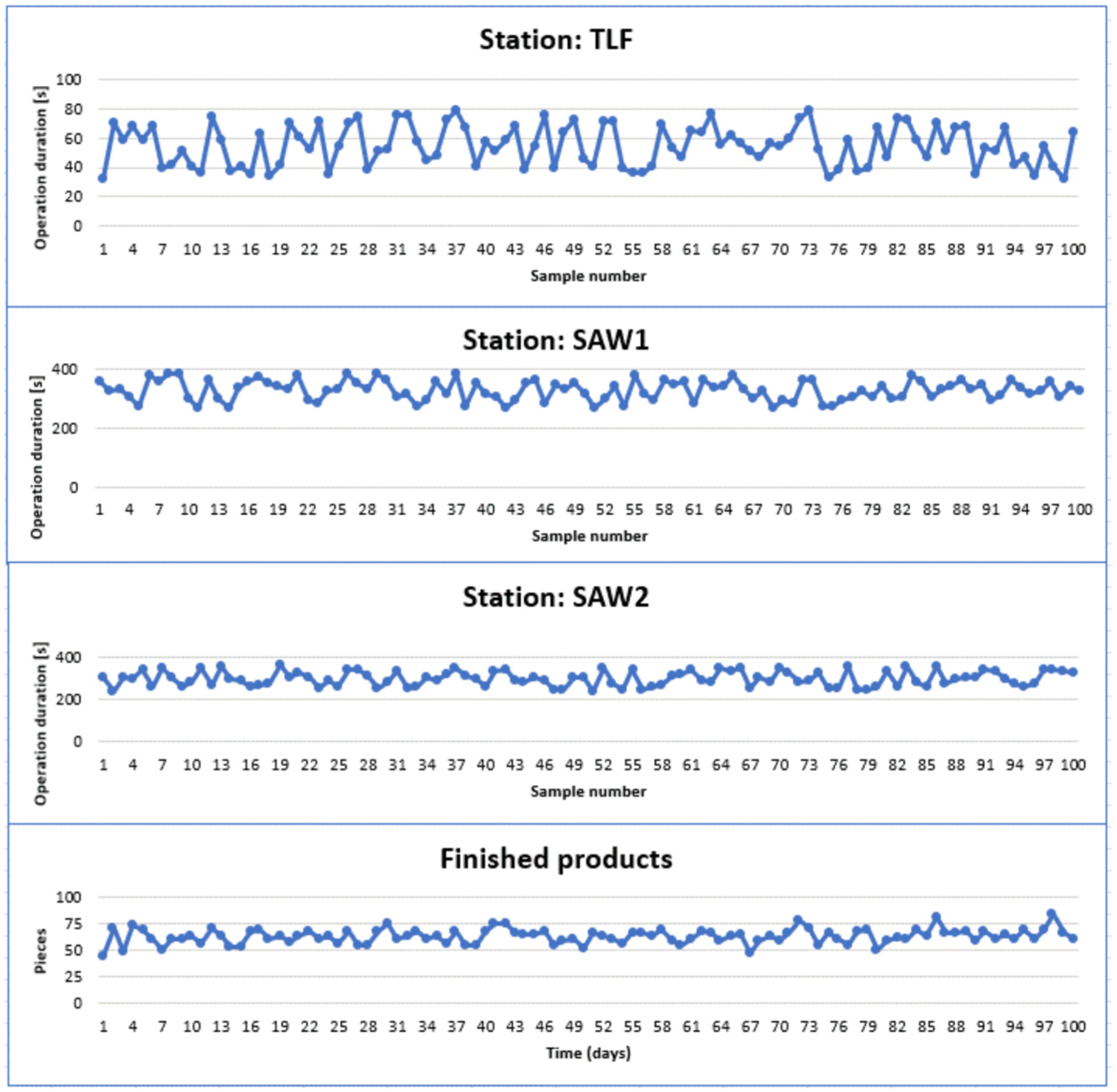
A summary of the obtained results is presented in Figure 7.

Figure 7. Graphs of variation in operation duration at stations: TLF, SAW1, SAW2 (own study).

Analyzing the graphs (Figure 7), it can be noticed that the duration of individual operations is of varied nature. For the purposes of further work, basic descriptive statistics were generated in the Statistica environment based on the collected data (Table 2).

Table 2. Descriptive statistics for stations TLF, SAW1, SAW2 (own study).

Station	Mean	Median	Mode	Std. Dev.	Coef. Var.
TLF	54.78	54.61	54.61	13.73	25.06
SAW1	328.10	330.00	366.00	34.02	10.37
SAW2	297.50	298.50	298.50	35.56	11.96

During the numerical analysis in the Statistica environment, a report of the best-fitting probabilistic model was generated for the obtained results and of the Anderson–Darling significance test performed (Table 3).

Table 3. Results of the probabilistic distribution fitting analysis against the Anderson–Darling test for the TLF, SAW1, SAW2 stations (own study).

	AD p-Value Distribution Summary Ranked by: Anderson–Darling
Station	Normal	Log-Normal	Weibull	Triangular	Rayleigh	Johnson
TLF	0.156658	0.115502	0.167748	-	0.000002	-
SAW1	0.249477	0.211876	0.238758	-	-	-
SAW2	0.890936	0.607907	0.672668	0.179467	-	-

The p-value for Anderson–Darling analysis indicates how well a selected distribution model (e.g., Weibull) describes the actual behavior of the process—the higher the value, the better the distribution describes the relationship. This means that the statistics provide a better evaluation of the model’s fit to observations over the entire range.

The following notations were adopted to assess the fit of the distributions (Table 4):

Table 4. Assessment of the statistical distributions fit for the analyzed manufacturing processes of particleboard cutting in the Statistica software (own study).

Variant		Distribution
		Normal	Log Normal	Weibull	Triangular	Rayleigh	Johnson
Board_J	TLF	+	+	++	−	+	−
	Saw1	++	+	+	−	−	−
	Saw2	++	+	+	+	−	−

• very good fit (++),
• good fit (+),
• no fit (−).

The parameters used for the Weibull distribution (w is the current variate value for the Weibull distribution, p is the critical value of the distribution, and b is the scale parameter, c is the shape parameter) are presented in Table 5.

Table 5. Parameters for selected distributions—Weibull (own study).

	w	p	b	c
TLF-Weibull	1.3856294	0.75	60.1169	4.5721

The parameters used for the normal distribution (z is the current variate value for the normal distribution, p is the critical value of the distribution, and b is the scale parameter) are presented in Table 6.

Table 6. Parameters for selected distributions—normal (own study).

	z	p	Location	b
Saw1-Normal	0.674490	0.75	328.14	32.0235
Saw2-Normal	0.674490	0.75	297.47	35.5654

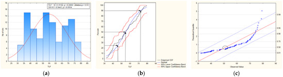
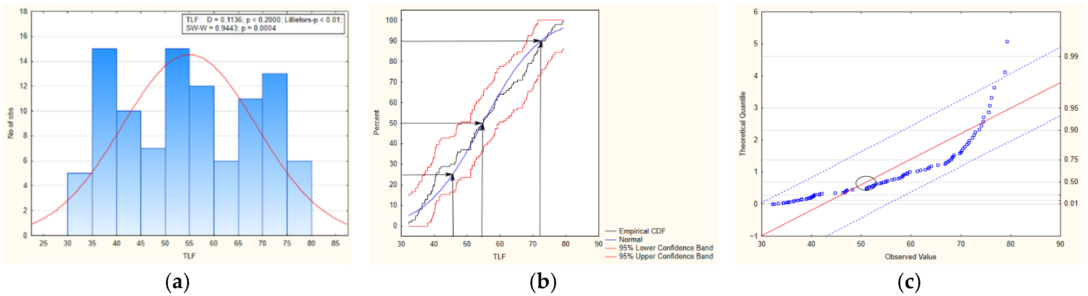
Analyzing the data presented in Figure 8 for the TLF station, it can be concluded that the variability of the probability estimation characteristics is at the level of α = 0.05 of the handling operation duration at the TLF station.

Figure 8. Diagrams of statistical analyses of TLF, (a) histogram, (b) empirical cumulative distribution function, (c) probabilistic model of the Weibull distribution (own study).

In the context of the obtained statistics, it should be observed that no more than 25% of the duration times are shorter than or equal to 45 s, which should be interpreted as a very optimistic estimation of the duration of the handling activity at the analyzed station. For the 50% probability level, most recommended for manufacturing processes, as determined from the percentile grid, the estimated duration of the operation is less than or equal to 55 s. The values at the 50% percentile level coincide with the statistics of the mean values (Table 1). In industrial practice, this probability level is most often recommended. In the upper pessimistic estimate, at the 90% percentile line, it can be assumed that 10% of operation durations take no less than 72 s.

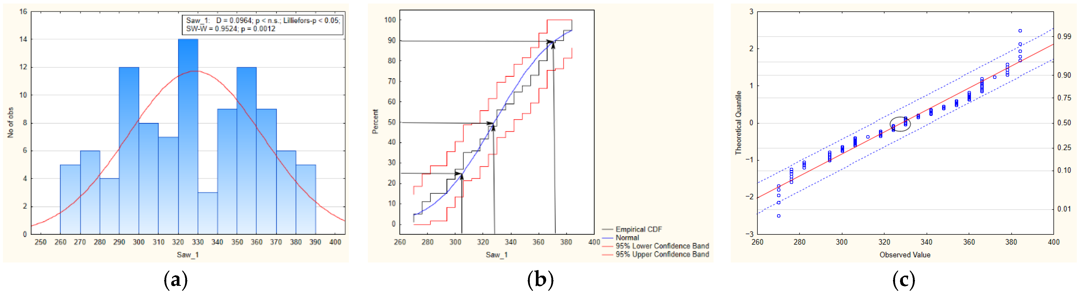
Analyzing the data presented in Figure 9 for the SAW1 station, it can be concluded that the variability of the probability estimation characteristics is at the level of α = 0.05 of the board cutting operation duration.

Figure 9. Diagrams of statistical analyses of SAW1: (a) histogram, (b) empirical cumulative distribution function, (c) probabilistic model of the normal distribution (own study).

In the context of the obtained statistics, it should be observed that no more than 25% of the duration times are shorter than or equal to 306 s, which should be interpreted as a very optimistic estimation of the duration of the handling activity at the station. For the 50% probability level, as determined from the percentile grid, the estimated duration of the operation is less than or equal to 328 s. In the upper pessimistic estimate, at the 90% percentile line, it can be assumed that 10% of operation durations take no less than 369 s.

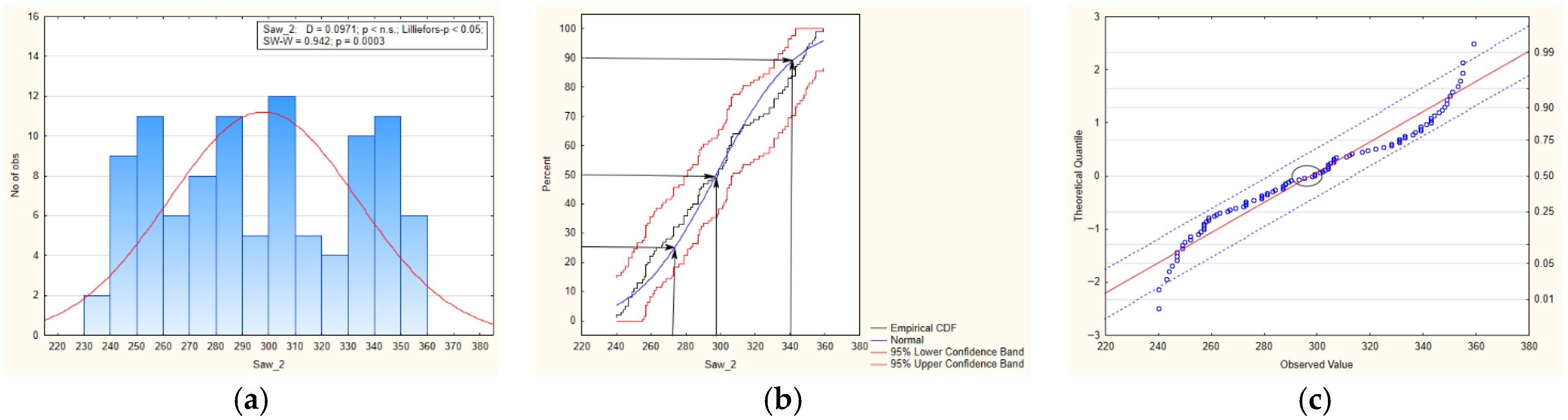
Analyzing the data presented in Figure 10 for the SAW2 station, it can be concluded that the variability of the probability estimation characteristics is at the level of α = 0.05 of the cutting operation duration.

Figure 10. Diagrams of statistical analyses of SAW2, (a) histogram, (b) empirical cumulative distribution function, (c) probabilistic model of the normal distribution (own study).

In the context of the obtained statistics, it should be observed that no more than 25% of the duration times are shorter than or equal to 272 s, which should be interpreted as a very optimistic estimation of the duration of the handling activity at the analyzed station. For the 50% probability level, as determined from the percentile grid, the estimated duration of the operation is less than or equal to 298 s, which corresponds to the average value of the durations obtained. In the upper pessimistic estimate, at the 90% percentile line, it can be assumed that 10% of operation durations take no less than 340 s.

Assuming a probability of 25% means a very high uncertainty of completing the technological process within the specified time, while assuming a probability value of 90%, as determined on the percentile grid, means a pessimistic assumption of completing the technological process. Assuming a 50% probability means the recommended probability of completing the operation within the designated technological time. In light of the obtained distributions and their analysis, it can be stated that the data “are arranged” along a straight line. This proves that the probabilistic model was correctly selected in all possible cases, and the nature of the distribution shows no disruptions to the technological operation being conducted. With stable operation of the machines and proper setting of controls, the technological processes described in the paper can be classified as random stationary processes. The adopted assumptions are confirmed by the determined probabilistic models based on the normal distribution; in the case of the Weibull distribution, it should also be assumed that the analyzed technological process is random in nature, but in this particular case, certain types of fluctuations related to picking of material and its downstream transport can be identified. The technologist controlling the process should know the effects of changes in the set of conditions of individual process stages.

The above graphs of probabilistic model fitting use the graphical method to present grouping of results in the form of points on both sides of the designated simple graphs, the occurrence being caused by the fluctuation of the duration of individual technological operations, as well as the specificity of the manufacturing process. Based on the estimated parameters of statistical models (Table 3 and Table 4), simulation models were developed using the FlexSim software to enable the technological identification. They take into account the basic statistical parameters of the duration of individual operations, their probability density function and the cumulative distribution function. The presented statistics describe the analyzed technological processes very accurately (Figure 8, Figure 9 and Figure 10).

The statistics were used to determine the settings for the simulation assuming the production capacity level at 25%, 50% and 90% probability of estimating the duration of the technological operation.

6. Running the Simulation Program and Analyzing the Results

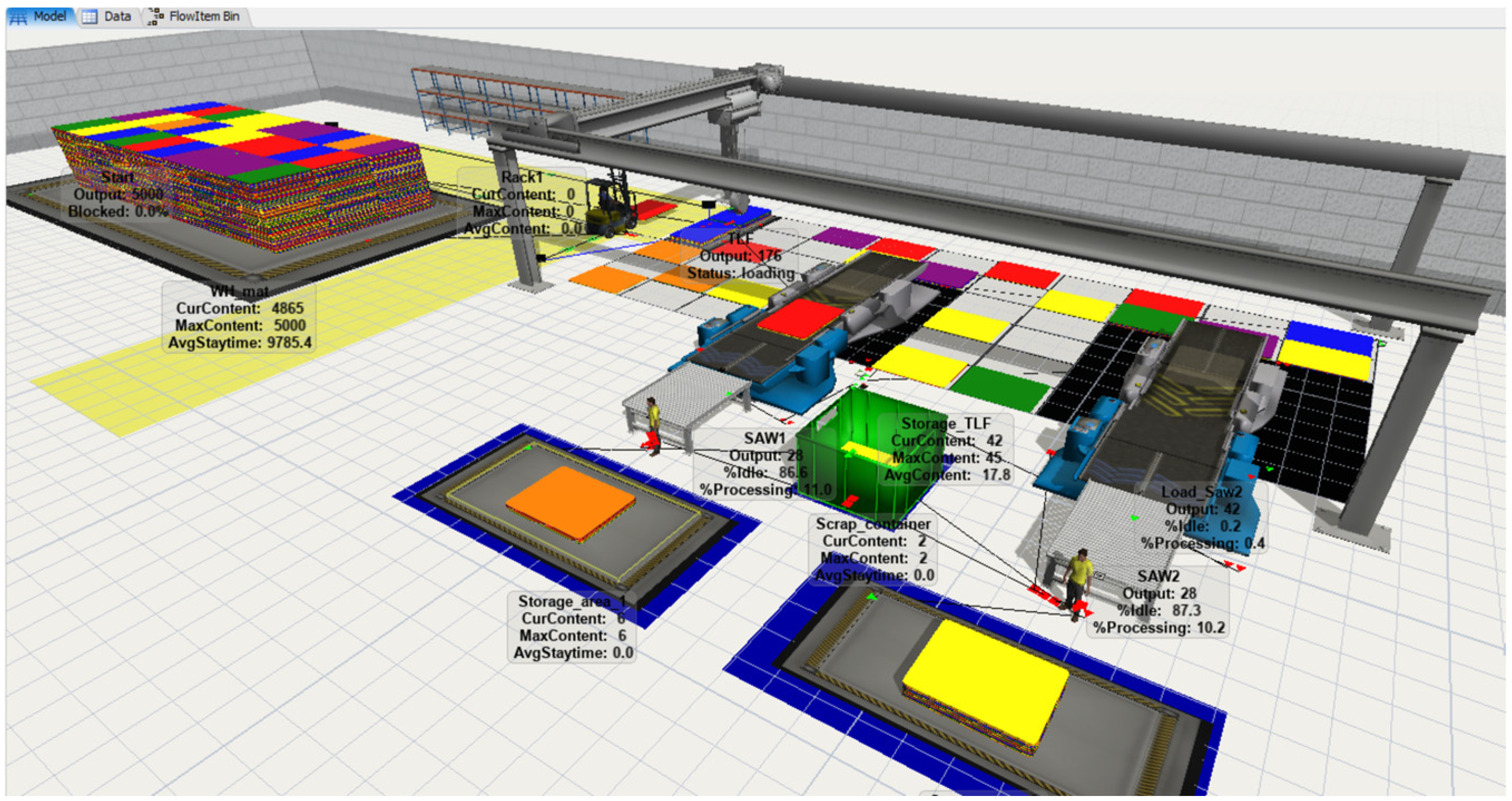
The simulation (Figure 11) was performed for 1, 2 and 3 shifts, assuming that the shift duration is 8 h. The simulation duration was assumed to be eight hours for each shift, excluding the system warm-up phase.

Figure 11. Computer simulation of the analyzed manufacturing system in the FlexSim environment on the run (own study).

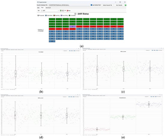
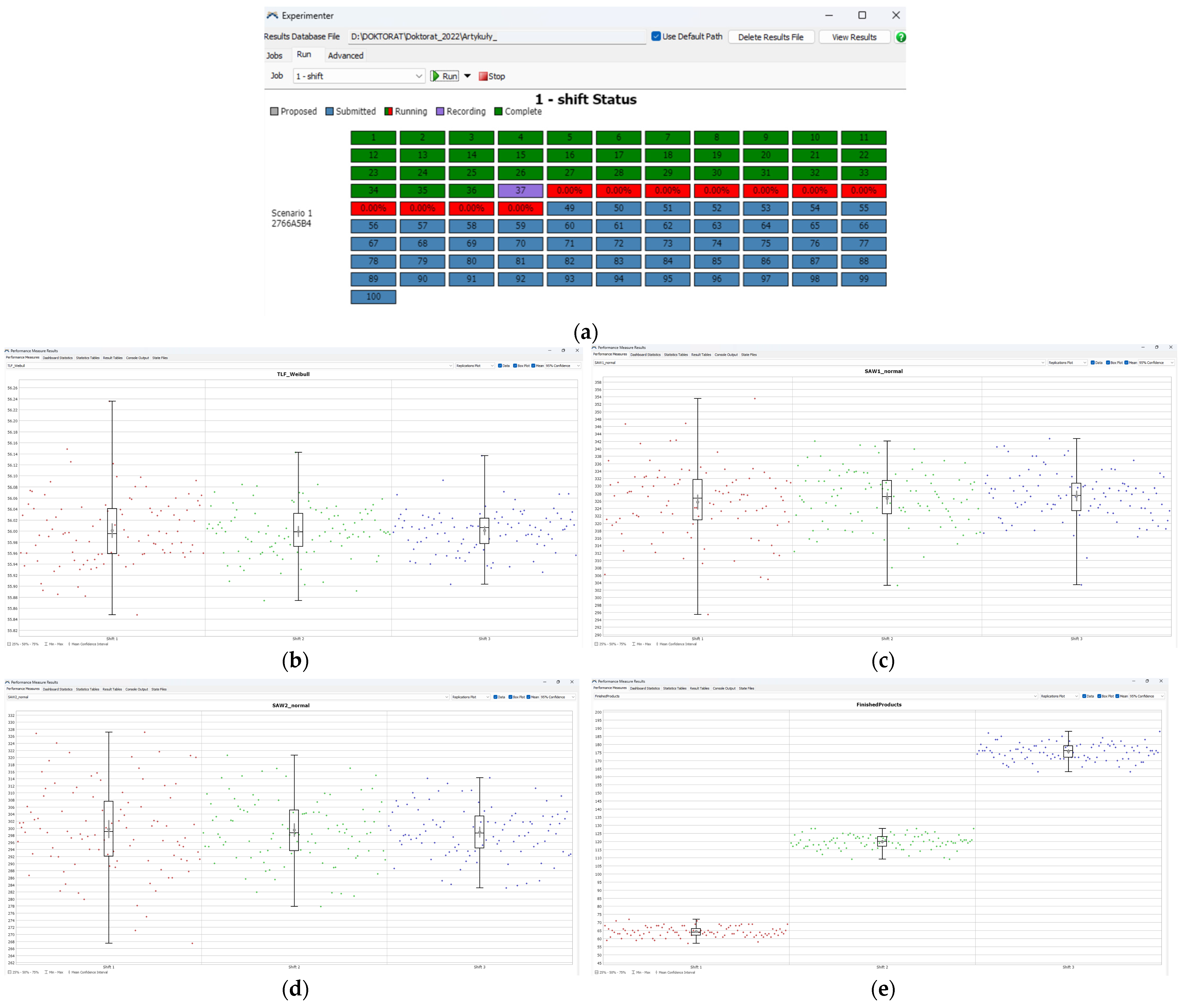
A graphical representation of the time series obtained in the simulation by replication is presented in Figure 12. As part of the simulation replication, three states of the plant operation were calculated, i.e., a single-shift system (8 h) and, as part of the simulation experiment, the second (16 h) and third shift (24 h).

Figure 12. Graphs of variation in operation duration at stations: TLF (b), SAW1 (c), SAW2 (d) and finished products (e) after simulation for each of 3 shifts after 36 of 100 replications (a) (own study).

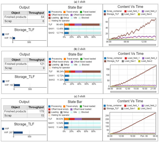
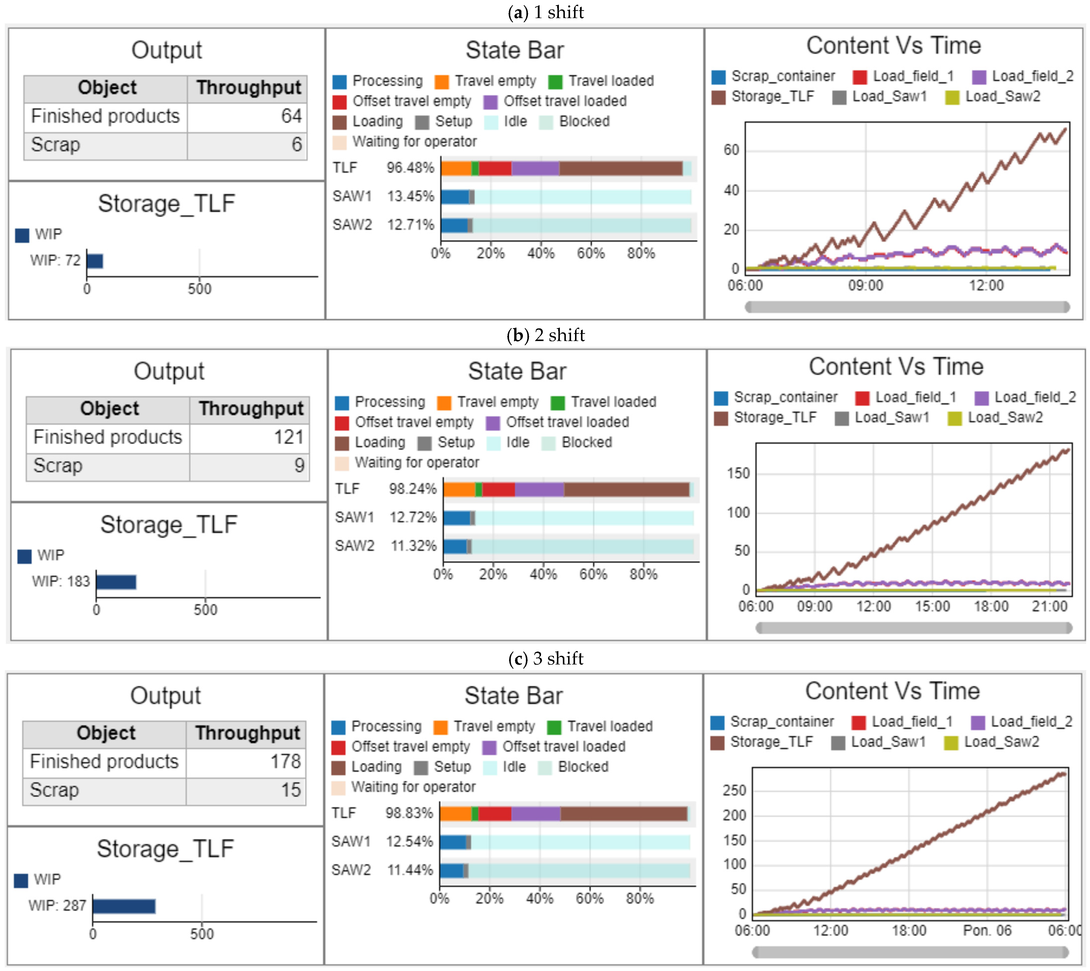
Figure 13 presents simulation reports for each work shift, summarizing the number of finished boards ready for assembly, the number of scrap boards, the filling of the TLF storage buffer, the workstation loads and the material build-up over time.

Figure 13. Generated simulation data reports assuming 50% probability of operation duration for: (a) dashboard—1 shift, (b) dashboard—2 shifts, (c) dashboard—3 shifts (own study).

The generated results for all considered variants based on the simulation reports are summarized in Table 7, Table 8 and Table 9. Estimating the probability of 50% of the duration of technological operations in the discussed process for 3 shifts, 178 finished sets of components for cabinet assembly will be produced, and in the presented description, post-production scrap in the form of 15 particleboards will be created, while the TLF storage will have a stock of material in the amount of 287 boards.

Table 7. Results of computer simulation analyses related to estimating the duration of production processes (own study).

Pα = 0.05	Station			Shift	Output (pcs.)	Scrap (pcs.)	WIP TLF (pcs.)
	TLF	SAW1	SAW2
90%	72 s	369 s	340 s	1	46	3	89
				2	77	7	218
				3	110	9	362
50%	55 s	328 s	298 s	1	64	6	72
				2	121	9	183
				3	178	15	287
25%	45 s	306 s	272 s	1	77	7	53
				2	157	11	137
				3	228	24	212

Table 8. Statistics for actual measurements of operations and pieces produced for results obtained in simulations.

Pα = 0.05	Real Data	Simulation Data	t-Student Statistics
			t	tcrit
	TLF
Time	55 s	56 s	0.3735	1.9599
	SAW1
	328 s	326 s	0.4818	1.9599
	SAW2
	298 s	300 s	0.5452	1.9599
	Finished products
Pcs.	63	64	0.1181	1.9599

Table 9. Loads of production stations related to the estimation of the duration of production processes (own study).

Pα = 0.05	Shift	TLF [%]	SAW1 [%]	SAW2 [%]
Usage, P = 90%	1	96.48	9.98	9.81
	2	98.24	8.87	8.49
	3	98.83	8.46	7.97
Usage, P = 50%	1	96.48	13.45	12.71
	2	98.24	12.72	11.32
	3	98.83	12.54	11.44
Usage, P = 25%	1	96.48	15.11	14.71
	2	98.24	15.16	13.98
	3	98.83	15.24	14.21

Validation of simulation models

In order to check whether there are statistically significant differences between the mean values obtained in actual production conditions and the mean values obtained in the simulation, a test for the two means was performed [26,33].

The two-sample means test was performed against actual measurements and simulation results at a probability level of 50%. The results of the statistical analyses are presented in Table 8.

Analyzing the statistical data [38] presented in the table, it can be concluded that there are no statistically significant differences in the obtained mean values determined for 100 records from the company data [37] carried out over a period of 6 months and obtained for 100 replications as a result of simulation for production stations (TLF, SAW1, SAW2) and final products. It should be noted that the actual data came from the production of one shift, from 6:00 a.m. to 2:00 p.m. on weekdays. During the research work, simulations in the FlexSim environment for the second and third shifts were carried out, assuming probability levels of 25%, 50% and 90%.

Based on the results from the simulation report (Figure 13), the loads of individual stations for 3 shifts were determined and summarized in Table 9. Estimating the probability of 50% of the duration of technological operations in the discussed process for 3 shifts, the load of the TLF automatic feeding storage system is 98.83%, for the SAW1 panel saw station it is 12.54%, and 11.44% for the SAW2 panel saw station.

7. Discussion

A review and analysis of the subject literature indicate numerous works (Table 1) utilizing simulation modeling to solve specific production problems. However, in the context of estimating production capacity, models based on deterministic assumptions or statistical simplifications (e.g., the use of mean cycle time) are dominant. Such an approach generates only an ‘average’ picture or an ‘expected scenario,’ overlooking the inherent variability of processes. In particular, there is a distinct research gap regarding simulation models that explicitly and comprehensively link the probability distribution of technological operation durations with a probabilistic estimate of production capacity. This capacity should be understood not as a single figure, but as a distribution function or an interval with a specified confidence level. The lack of models directly integrating advanced analysis of operation time distributions with a quantitative assessment of system capacity leads to the widespread application of simplified, deterministic methods. The consequence is an inability to adequately account for the real risks and uncertainties associated with actual production capabilities.

The analyzed literature lacks an evaluation of results obtained from replications performed within the FlexSim environment. Furthermore, no statistical analyses were found that would verify the significance of models developed using replication data. Yet, such data, acquired through simulation, constitute a key foundation for reliable validation. They enable a direct and quantitative comparison of results obtained under real-world conditions with those derived from computer simulation. Analyzing the data resulting from technological processes, it can be concluded that the relatively low load of the SAW1 and SAW2 stations is caused by the long waiting time for material from the TLF station, which is a bottleneck of the process. Identification of the bottleneck is essential for introducing improvements to the analyzed technological process. The load assessment at SAW1 and SAW2 stations highlights the unused production capacity of the saws. It should be verified whether the use of both saw stations is justified in the considered case. When cutting homogeneous materials, switching off one of the machines may prove to be a solution that increases the load on the other machine. In industrial practice, however, this type of solution may prove unreliable. Taking action to reduce the workload of one of the stations is a choice of the lesser evil. When cutting materials of similar dimensions, it is recommended to exclude the SAW2 saw.

The use of probabilistic models enables the identification of production capabilities that account for the inherent variability of the processes in the production line. This information is useful when making decisions about launching more production shifts, assessing production capacity and their effectiveness. When modeling the duration of production processes, three scenarios can be assumed: optimistic, realistic and pessimistic. These are differentiated based on the coefficients of variation and the organizational context of individual changes. The optimistic scenario (corresponding to a quantile below 50%) can be used for the first shift, assuming a lower probability of deviations from the mean process durations—resulting, for example, from higher qualifications and experience of staff and more favorable ergonomic conditions (e.g., time of day conducive to concentration and efficiency). The pessimistic scenario (quantile above 50%) may be assigned to the third shift, due to the potentially higher risk of errors and disruptions associated with night work (fatigue, lower availability of technical support, reduced alertness). The realistic scenario (50% quantile, i.e., the median of the distribution) is a reference point and can be used for the second shift, representing typical, average operating conditions of the production system.

The obtained statistics on the probability of production implementation within a given time horizon constitute key input for the decision-making processes regarding multi-shift planning, resource allocation and optimization of production capacity utilization. In particular, they enable rational decision-making as to whether additional production shifts are to be launched or if the current single-shift cycle is to be maintained, based on the forecasted uncertainty of order fulfillment. In the context of dynamically changing demand and shortening lead times, having reliable risk estimates of failure to complete production within the required time becomes a strategic factor in ensuring timely order delivery. A company may consciously accept the production risk associated with accepting orders with short lead times, but such a decision should be preceded by an analysis of the consequences—including potential costs related to late delivery, loss of reputation or failure to meet contractual obligations.

The proposed methodological approach—based on probabilistic modeling of time-variable production processes—can be consistently applied to subsequent stations and operations within the entire production line, thus enabling scaling of the risk analysis, identification of bottlenecks in terms of execution uncertainty, and a synthesis of a coherent, multi-stage predictive model to be used for production planning and control purposes.

8. Conclusions

The use of a properly developed computer simulation model to analyze a manufacturing system enables obtaining valuable information on its operation. Based on the virtual environment designed in this way, it is possible to conduct research on, among others, production capacity depending on given parameters, e.g., the probability of random events. Proper identification of such phenomena, including the development of appropriate statistical and probabilistic models for processes, can significantly improve the planning process of order completion. Production planning in the startup phase using probabilistic models becomes crucial due to the non-linear nature of the bathtub curve, which models the increased risk of failures, process errors and deviations from nominal operation durations during the initial period of system operation. Appropriate modeling of this risk through probability distributions enables realistic estimation of shift-planning uncertainty and supports decision-making based on the forecasted probability of meeting production deadlines. This type of approach has not been implemented before. Based on probabilistic models, it is possible to assume an optimistic production variant as well as a pessimistic one regarding the probability of process completion assuming long durations of manufacture. A virtual factory model with appropriate random event characteristics is able to verify the smoothness of production, determine its weak points and provide feedback on the effects of planned changes aimed at improving a specific process. This type of approach is extremely important in the case of new technological lines, for which the production dynamics may have the characteristics of operating machines related to an early age. However, this requires that the user properly identifies the processes taking place in this production environment, has good knowledge of the correct approach to building simulation models and conducting experiments on them.

Based on the complete simulation model, a simulation of the furniture component production process was performed with variable probability estimation in order to define the efficiency of the production line, based on statistical and probabilistic models. The conducted process identification allows for building the simulation models and the development of designs of experiments for complex technological processes supporting decision-making processes in the enterprise.

References

- Ingaldi, M.; Ulewicz, R. Problems with the Implementation of Industry 4.0 in Enterprises from the SME Sector. Sustainability 2020, 12, 217. [Google Scholar] [CrossRef] [Scilit]
- Kolny, D.; Drobina, R. Modelowanie i symulacja procesu rozkroju płyty wiórowej w programie Arena. In Technologie, Procesy i Systemy Produkcyjne’2022; Rysiński, J., Więcek, D., Eds.; Wydawnictwo Naukowe Akademii Techniczno-Humanistycznej w Bielsku-Białej: Bielsko-Biała, Poland, 2022. [Google Scholar] [CrossRef] [Scilit]
- Florek-Paszkowska, A.; Cymanow, P. Zarządzanie procesem produkcji z wykorzystaniem metody AHP/ANP. Metod. Ilościowe W Badaniach Ekon. 2012, 13, 96–105. [Google Scholar]
- Jurczyk, K.; Wzorek, A. Modelowanie i symulacja systemów produkcyjnych przy wykorzystaniu oprogramowania Flexsim-studium przypadku. Stud. Proc. Pol. Assoc. Knowl. Manag. 2018, 87, 4–20. [Google Scholar]
- Drobina, R. Probabilistic Model of Fatigue Strength. Fibres Text. East. Eur. 2013, 3, 61–67. [Google Scholar]
- Reussner, R.H.; Schmidt, H.W.; Poernomo, I.H. Reliability prediction for component-based software architectures. J. Syst. Softw. 2003, 66, 241–252. [Google Scholar] [CrossRef] [Scilit]
- Nurprihatin, F.; Angely, M.; Tannady, H. Total productive maintenance policy to increase effectiveness and maintenance performance using overall equipment effectiveness. J. Appl. Res. Ind. Eng. 2019, 6, 184–199. [Google Scholar]
- Małopolski, W. Modelowanie i optymalizacja systemów wytwarzania w programie arena. Czas. Tech. Mech. 2012, 109, 91–108. [Google Scholar]
- Łatuszyńska, M. Modelowanie i symulacja w zarządzaniu produkcją. Przegląd Organ. 2015, 12, 51–57. [Google Scholar] [CrossRef] [Scilit]
- Kolny, D.; Kaczmar-Kolny, E.; Dulina, Ľ. Modeling and simulation of the furniture manufacturing and assembly process in the arena simulation software. Technol. Autom. Montażu 2023, 119, 13–22. [Google Scholar] [CrossRef] [Scilit]
- Twardochleb, M. Metody modelowania statystycznego a optymalizacja funkcji wielu zmiennych z ograniczeniami. In VII Naukowa Sesja Informatyki 2002; Politechnika Szczecińska: Szczecin, Poland, 2022. [Google Scholar]
- Chomać-Pietrzecka, E. Probabilistyczne ujęcie metod ilościowych w analizie wartości przedsiębiorstwa. Finans. Rynk. Finans. Ubezpieczenia 2011, 47, 11–24. [Google Scholar]
- Plucińska, A.; Pluciński, E. Probabilistyka. In Rachunek Prawdopodobieństwa, Statystyka Matematyczna, Procesy Stochastyczne; Wydawnictwo WNT: Warsaw, Poland, 2000; p. 13. [Google Scholar]
- Beaverstock, M.; Greenwood, A.; Nordgren, W. Symulacja stosowana. In Modelowanie i Analiza Przy Wykorzystaniu FlexSim, 2nd ed.; Wydawnictwo InterMarium: Cracow, Poland, 2019. [Google Scholar]
- Ciszak, O. Komputerowo wspomagane modelowanie i symulacja procesów produkcyjnych. Zesz. Nauk. Politech. Poznańskiej 2007, 6, 39–45. [Google Scholar]
- Kritzinger, W.; Karner, M.; Traar, G.; Henjes, J.; Sihn, W. Digital Twin in manufacturing: A categorical literature review and classification. Ifac-PapersOnline 2018, 51, 1016–1022. [Google Scholar] [CrossRef] [Scilit]
- Florescu, A.; Barabas, S.A. Modeling and simulation of a flexible manufacturing system—A basic component of industry 4.0. Appl. Sci. 2020, 10, 8300. [Google Scholar] [CrossRef] [Scilit]
- Lewicki, W.; Niekurzak, M.; Wróbel, J. Development of a Simulation Model to Improve the Functioning of Production Processes Using the FlexSim Tool. Appl. Sci. 2024, 14, 6957. [Google Scholar] [CrossRef] [Scilit]
- Mokshin, V.V.; Kirpichnikov, A.P.; Soiko, A.I. Simulation and optimization of the cargo terminal in the AnyLogic environment. J. Phys. Conf. Ser. 2019, 4, 1368. [Google Scholar] [CrossRef] [Scilit]
- Kikolski, M. Identification of production bottlenecks with the use of Plant Simulation software. Ekon. Zarz. 2016, 8, 103–112. [Google Scholar] [CrossRef] [Scilit]
- Zaayman, G.; Innamorato, A. The application of simio scheduling in industry 4.0. In 2017 Winter Simulation Conference (WSC); IEEE: Las Vegas, NV, USA, 2017; pp. 4425–4434. [Google Scholar] [CrossRef] [Scilit]
- Alot, Z. Modele statystyczne procesów logistycznych dla potrzeb ich oceny i kontroli. Logistyka 2014, 3, 34–43. [Google Scholar]
- Czabak-Górska, I.D.; Kucińska-Landwójtowicz, A. Identyfikacja zaburzeń procesu produkcyjnego w oparciu o analizę błędów grubych—Studium przypadku. In Innowacje w Zarządzaniu i Inżynierii Produkcji; Knosala, R., Ed.; Oficyna Wydawnicza Polskiego Towarzystwa Zarządzania Produkcją: Opole, Poland, 2015; pp. 246–256. [Google Scholar]
- Czader, W.; Szpoczek, E. Komputerowo wspomagane statystyczne sterowanie procesu. Mechanik 2015, 88, 131–138. [Google Scholar]
- Drobina, R. Probabilistic Model of the Fatigue Durability of Knitted Fabrics Produced from Standard Smooth and Fancy Flame Cotton Yarns. Fibres Text. East. Eur. 2013, 4, 75–84. [Google Scholar]
- StatSoft, 2025, Elektroniczny Podręcznik Statystyki PL, Krakow. Available online: http://www.statsoft.pl/textbook/stathome.html (accessed on 1 December 2025).
- Weibull, W. A statistical theory of the strength of materials. R. Inst. Engng Res. 1939, 151, 45. [Google Scholar]
- Weibull, W. A statistical representation of fatigue failures in solids. Trans. R. Inst. Technol. 1949, 27, 50. [Google Scholar]
- Weibull, W. A statistical distribution function of wide application. J. Appl. Mech. 1951, 18, 293. [Google Scholar] [CrossRef] [Scilit]
- Li, H.; Foschi, R.; Vaziri, R.; Fernlund, G.; Poursartip, A. Probability-based modelling of composites manufacturing and its application to optimal process design. J. Compos. Mater. 2002, 36, 1967–1991. [Google Scholar] [CrossRef] [Scilit]
- Afolabi, K.; Akintayo, B.; Babatunde, O.; Kareem, U.A.; Ogbemhe, J.; Ighravwe, D.; Oludolapo, O. Stochastic Optimization of Quality Assurance Systems in Manufacturing: Integrating Robust and Probabilistic Models for Enhanced Process Performance and Product Reliability. J. Manuf. Mater. Process. 2025, 9, 250. [Google Scholar] [CrossRef] [Scilit]
- Mańczak, K. Metody Identyfikacji Wielowymiarowych Obiektów Sterowania; Wydawnictwo WNT: Warsaw, Poland, 1979. [Google Scholar]
- Stanisz, A. Przystępny Kurs Statystyki na Przykładach z Medycyny z Wykorzystaniem Programu STATISTICA, 2nd ed.; Statsoft: Cracow, Poland, 2006; Volume I. [Google Scholar]
- Stanisz, A. Przystępny Kurs Statystyki na Przykładach z Medycyny z Wykorzystaniem Programu STATISTICA, 2nd ed.; Statsoft: Cracow, Poland, 2006; Volume II. [Google Scholar]
- Benjamin, J.R.; Cornell, C.A. The Calculus of Probability, Mathematical Statistics and the Theory of the Decision for Engineers; Wydawnictwo WNT: Warsaw, Poland, 1977. [Google Scholar]
- Karkula, M. Modelowanie i Symulacja Procesów Logistycznych; Wydawnictwa Akademii Górniczo-Hutniczej im. Stanisława Staszica: Cracow, Poland, 2013. [Google Scholar]
- Unpublished Archival Data, ATEPAA® Group. Available online: https://www.atepaa.com/pl (accessed on 1 October 2022).
- Iwaniec, M. Normy I jakość z Pakietem Statistica: Od Kontroli Odbiorczej po Six Sigma, Stasoft. Available online: https://media.statsoft.pl/_old_dnn/downloads/normy_i_jakosc.pdf (accessed on 1 December 2025).
Disclaimer/Publisher’s Note: The statements, opinions and data contained in all publications are solely those of the individual author(s) and contributor(s) and not of MDPI and/or the editor(s). MDPI and/or the editor(s) disclaim responsibility for any injury to people or property resulting from any ideas, methods, instructions or products referred to in the content. |
© 2026 by the authors. Licensee MDPI, Basel, Switzerland. This article is an open access article distributed under the terms and conditions of the Creative Commons Attribution (CC BY) license.