


Featured Application
This study presents a leakage-controlled framework for examining whether EHG recordings obtained during earlier and later pregnancy periods can be distinguished using wavelet-scalogram representations. All records and overlapping segments from the same pregnancy are kept within the same validation fold, and segment-level predictions are aggregated at the record level before the representation-specific outputs are combined through probability-level fusion. The framework is intended for reproducible analysis of recording-period-related differences in ICEHG DS. It is not designed to predict preterm birth, delivery outcome, or clinical diagnosis. Independent validation in external, outcome-defined, and longitudinal pregnancy cohorts is required before broader physiological or clinical interpretations can be made.
Abstract
Electrohysterography (EHG) provides a non-invasive measure of uterine electrical activity. Splitting overlapping segments or paired pregnancy recordings between training and test sets can bias deep learning evaluation. We evaluated a pregnancy-wise, leakage-controlled framework for distinguishing early- from later-recorded observations in the Induced Cesarean Electrohysterogram Dataset (ICEHG DS). The dataset comprised 126 records from 91 pregnancies: 35 with paired early and later recordings and 56 with one recording. The S1, S2, and S3 channels were band-pass filtered, segmented into overlapping 120-s windows, and converted to wavelet scalograms. Separate CNN–Transformer models were trained for each channel and a synchronized red–green–blue (RGB) representation. Segment probabilities were averaged within each record, and representation-specific probabilities were combined using a five-outer/three-inner nested GroupKFold design. The optimized ensemble achieved a mean outer-fold raw ROC-AUC of 0.804 ± 0.062 (95% CI: 0.725–0.880), accuracy of 0.635, sensitivity of 0.919, specificity of 0.359, and balanced accuracy of 0.639. Equal-weight four-representation fusion was numerically highest (0.807 ± 0.069); optimized weighting showed no advantage. In 30/35 paired pregnancies (85.7%; exact 95% CI: 69.7–95.2%), early recordings received higher raw early-class scores (sign-test p = 2.24 × 10⁻⁵), without establishing physiological changes or clinical utility. External longitudinal validation is required.
1. Introduction
Preterm birth—defined as delivery before 37 completed weeks of gestation—remains a severe global burden in maternal and neonatal healthcare [1]. Recent estimates indicate that approximately 13.4 million infants were born preterm in 2020, representing nearly 10% of all live births worldwide [2]. While modern neonatal intensive care has improved survival rates, these infants face significant risks of acute mortality alongside long-term neurodevelopmental, respiratory, and learning difficulties [3]. Addressing these complications requires objective, non-invasive methods to monitor gestational adaptations and uterine dynamics.
Assessment of threatened preterm labor typically combines maternal and obstetric history with contraction monitoring, cervical examination, cervical-length measurement, biochemical markers, and clinical symptoms. However, these conventional measures provide limited direct insight into the electrophysiological processes involved in myometrial activation [4]. Electrohysterography (EHG) offers a different perspective by recording uterine electrical activity non-invasively from electrodes placed on the maternal abdomen. Uterine contractions originate from electrical activity in myometrial cells, whose excitability, intercellular coupling, and signal-propagation properties change as pregnancy progresses toward labor [5]. EHG can therefore complement conventional clinical observations with information about uterine electrophysiology.
Previous studies have reported changes in EHG characteristics across gestation and labor-related states. For instance, Leman et al. examined abdominal EHG recordings from high-risk pregnancies and reported variation in contraction-related electrical characteristics over the course of pregnancy [6]. Lucovnik et al. found that uterine electromyography (EMG) propagation velocity increased near labor and evaluated its combination with peak power-spectrum frequency for identifying women who delivered prematurely within seven days in their study population [7]. Similarly, Fele-Žorž et al. assessed linear and nonlinear EHG characteristics and identified spectral and entropy-based measures that differed between term and preterm delivery groups [8]. These findings show that EHG characteristics vary with gestational and labor-related conditions, but they do not establish that recording time alone produces electrophysiological signatures that are independent of pregnancy outcome.
Open-access EHG datasets have supported the evaluation of signal-processing and classification methods across different obstetric settings. The Term–Preterm EHG Database (TPEHG DB), derived from the work of Fele-Žorž et al. [8], contains 300 three-channel recordings. Alexandersson et al. introduced the Icelandic 16-electrode EHG database, which provides spatially distributed multichannel recordings acquired during pregnancy and active labor [9]. Jager et al. subsequently characterized records from the TPEHG DB and the Term–Preterm EHG DataSet with Tocogram (TPEHGT DS), including contraction and non-contraction intervals [10]. More recently, Jager published the Induced Cesarean Electrohysterogram Dataset (ICEHG DS), which comprises 126 approximately 30-min EHG recordings from 91 pregnancies ending in induced, cesarean, or induced-cesarean delivery [11].
To date, most computational EHG pipelines focus on binary classification tasks, namely term versus preterm delivery or labor versus non-labor states. Early architectures relied on hand-engineered temporal, spectral, nonlinear, and statistical parameters fed into shallow classifiers. Maner and Garfield validated the viability of artificial neural networks for labor identification using electromyographic variables [12], while Fergus et al. applied machine learning pipelines to the TPEHG DB, exploring minority-class oversampling to counter inherent class imbalances [13]. Subsequent studies noted that data-handling, sampling, and class-balancing protocols exert a strong influence on reported performance metrics. For example, Xu et al. demonstrated that optimized synthetic sampling for highly skewed EHG subsets shifts feature behavior and alters validation performance [14]. Such findings emphasize that analytical results remain inseparable from validation frameworks and data-handling choices.
Researchers have used several signal representations to examine the non-stationary behavior of uterine electrical activity. Xu et al. combined network-based analysis with frequency-domain measures and found that properties derived from EHG signals contributed to preterm-birth classification [15]. Because the spectral content of an EHG signal can change within a recording, time–frequency analysis provides a suitable way to examine these variations. Batista et al. developed a multichannel, multi-wavelet time–frequency framework for uterine electromyography [16]. Romero-Morales et al. subsequently evaluated continuous wavelet transform and entropy-derived characteristics for term–preterm classification and identified discriminative information in the tested EHG representations [17]. These studies support the use of wavelet-based time–frequency representations as an alternative to conventional handcrafted features, but they do not show that wavelet scalograms are inherently superior.
Deep learning can reduce reliance on handcrafted features by learning representations from raw EHG signals or time–frequency inputs. For instance, Fischer et al. evaluated end-to-end deep networks for assessing preterm birth risks, aiming to balance raw predictive capacity with model explainability [18]. Similarly, Goldsztejn and Nehorai combined spectral arrays with clinical metadata in hybrid deep learning models using the TPEHG DB and TPEHGT DS, which illustrated the distinct benefits of latent representation learning [19]. Nevertheless, increasing model complexity poses substantial overfitting risks, especially when the available training data spans a narrow pool of independent pregnancies. Comprehensive surveys of computational EHG models frequently highlight small sample cohorts, heterogeneous filtering choices, and loose validation loops as pervasive flaws in contemporary literature [20]. Indeed, a recent systematic review focusing on artificial intelligence in uterine dynamic modeling concluded that 86.7% of evaluated studies carried an unclear or high risk of bias, identifying the total absence of external validation as a primary roadblock to clinical adoption [21].
Recent advances in multi-view learning have extensively explored how divergences across heterogeneous data representations can be effectively managed via targeted feature selection and adaptive fusion mechanisms. For instance, Li et al. [22] introduced a balanced multi-view feature-selection framework tailored to mitigate class imbalance by minimizing differential information loss under rigorous regularization constraints. Concurrently, Li et al. [23] developed a quantum multi-view feature-selection paradigm that links configurable kernel circuits with adaptive fusion routines across diverse representations. Extending beyond conventional multi-view architectures, Li et al. [24] formulated an adaptive k-nearest-neighbor graph architecture that dynamically learns neighborhood selection parameters and sample weighting during the training trajectory. These studies provide broader methodological context for adaptive weighting. In our current study, this conceptual paradigm is applied to investigate standalone S1, S2, and S3 channels alongside synchronized RGB scalograms using both equal-weight pooling and inner-optimized probability fusion within a strict pregnancy-isolated validation architecture.
In this study, our objective moves away from traditional term–preterm or labor forecasting. Instead, we evaluate a methodological framework for distinguishing early-recorded from later-recorded EHG observations within the ICEHG DS while explicitly controlling pregnancy-level dependence. Because gestational age at acquisition is already known, the task is treated as a leakage-controlled recording-period benchmark rather than a clinical warning system or a direct test of longitudinal gestational physiology. The primary technical challenge involves controlling the overlapping analytical windows and the partially longitudinal structure of the dataset. Slicing continuous EHG tracks into overlapping blocks creates highly correlated sequences within a single session, leading to overly optimistic metrics if data splits are shuffled randomly. In addition, 126 records originate from only 91 pregnancies, including 35 pregnancies with paired early and later recordings. Therefore, every segment and all records linked to the same pregnancy must remain within the same validation partition to prevent cross-session leakage.
Preventing data leakage at the pregnancy level requires strict separation throughout the modeling pipeline. Feature fitting, early stopping limits, array-fusion tuning, probability calibration, and decision thresholds must be finalized without any influence from the target held-out test cohort. We address this via a five-outer/three-inner pregnancy-wise nested GroupKFold cross-validation framework. Within each inner fold, model fitting, early-stopping monitoring, and evaluation were performed using pregnancy-disjoint subsets. Predictions from the held-out inner-evaluation pregnancies were used to optimize ensemble fusion weights, calibrate probabilities, and select decision thresholds. The corresponding outer-test pregnancies remained excluded from all model development and configuration procedures. The primary discrimination metric was the arithmetic mean of the raw ROC-AUC values calculated independently across the five held-out outer folds. Sampling uncertainty was assessed using fold-stratified pregnancy-cluster bootstrap resampling. Importantly, pregnancy-wise separation protects evaluation integrity but does not by itself distinguish within-pregnancy gestational change from between-pregnancy heterogeneity in this partially longitudinal cohort.
Within this controlled loop, we treat the three bipolar ICEHG leads—S1, S2, and S3—as parallel representations of the recorded EHG signal. Channel-specific wavelet scalograms preserve representation-specific time–frequency structure, while temporally synchronized RGB matrices combine these inputs into a unified multichannel layout. Independent CNN–Transformer models were evaluated for the RGB, S1, S2, and S3 arrays, with segment-level scores averaged to obtain record-level outputs. Multi-representation fusion was then performed in probability space. Operationally, the framework extracted the fusion weights, Platt calibration parameters, and decision thresholds exclusively from the untouched inner-evaluation out-of-fold predictions, transferring them without modification to the corresponding held-out outer-test records. Because simple equal weighting was also evaluated, the analysis allows the incremental value of optimized weighting to be assessed rather than assumed.
The main methodological contribution of this study is the evaluation of multiple EHG representations within a validation framework that accounts for the partially longitudinal structure of the ICEHG DS. The dataset contains 126 EHG recordings from 91 pregnancies, including 35 pregnancies with paired early- and later-recorded observations and 56 pregnancies with a single recording. Consequently, recordings from the same pregnancy are not statistically independent and must remain within the same data partition. The CWT, CNN, and Transformer components are established methods; the contribution lies in integrating them into a pipeline designed to prevent pregnancy-level data leakage. The framework uses pregnancy-disjoint subsets for model fitting, early-stopping monitoring, and inner evaluation, followed by record-level temporal pooling and probability-level fusion. Under identical outer-test partitions, this design enables a consistent comparison of standalone channel models, uniform averaging, and inner-optimized fusion strategies without allowing recordings from the same pregnancy to appear in both development and test sets.
Accordingly, the primary methodological contributions of this work are organized as follows:
- •
- A pregnancy-wise nested GroupKFold validation architecture specifically tailored to the partially longitudinal ICEHG DS was established, separating network weight fitting, early-stopping checkpoints, untouched inner evaluations, and held-out outer testing while locking all multi-session tracks and overlapping windows from the same pregnancy into identical partitions.
- •
- Standalone S1, S2, S3, and synchronized RGB wavelet-scalogram inputs were benchmarked using dedicated CNN–Transformer backbones combined with record-level pooling.
- •
- Ensemble fusion weights, Platt calibration functions, and classification boundaries were derived exclusively from untouched inner-evaluation out-of-fold records and transferred without modification to held-out outer-test sets, retaining a simple equal-weight pooling strategy as a pre-specified simplicity benchmark.
- •
- Held-out performance was assessed using fold-specific ROC-AUC values and pregnancy-clustered uncertainty estimates, supplemented by paired-pregnancy analyses, CWT representation sensitivity experiments, conventional spectral baselines, and repeated-seed evaluations.
The findings presented hereafter therefore characterize leakage-controlled recording-period discrimination within the ICEHG DS cohort. While our paired-pregnancy analysis demonstrated a highly consistent intra-pregnancy ordering across the early-class scores in most matched recordings, this specific insight does not identify a unique physiological pathway of gestational maturation; furthermore, it must not be misinterpreted as verified performance for spontaneous preterm birth prediction, delivery pathway forecasting, or real-time clinical diagnosis. Independent evaluation in fully longitudinal, outcome-defined, and externally acquired pregnancy cohorts remains necessary before translating the observed discrimination into physiological or clinical conclusions.
2. Materials and Methods
Our methodological framework incorporated pregnancy-level cohort reconstruction, digital signal preprocessing, sliding-window segmentation, continuous wavelet transform (CWT) feature mapping, and representation-specific CNN–Transformer deep architectures. This workflow culminated in record-level temporal probability pooling managed within a pregnancy-wise nested validation design tailored for multi-representation fusion. All data-dependent configuration steps, including ensemble weight optimization, Platt probability calibration, and decision-threshold selection, were performed exclusively using inner out-of-fold predictions from the outer-development pregnancies. The corresponding outer-test pregnancies remained isolated throughout model development and configuration and were used only for final evaluation.
2.1. Dataset
This secondary analysis utilized the open-access Induced Cesarean Electrohysterogram Dataset (ICEHG DS), which was compiled at the University Medical Center Ljubljana, Slovenia, and hosted via PhysioNet. The dataset comprised 126 continuous, approximately 30-min surface EHG recordings obtained from 91 independent pregnancies. Within this pool, 62 tracks represented the early recording period (centered near the 23rd week of pregnancy), whereas the remaining 64 tracks captured the later recording period (centered near the 31st week). All evaluated pregnancies ended in induced, cesarean, or induced-cesarean delivery. Because these categorical labels mark the chronological timing of signal acquisition rather than clinical outcomes, the “early-recorded” and “later-recorded” groups reflect gestational ages and do not serve as proxies for preterm or term delivery categories.
The recording setup captured three distinct bipolar abdominal channels designated S1, S2, and S3. Four Ag/AgCl electrodes were positioned symmetrically above and below the umbilicus in two rows separated by 7 cm [11]. The bipolar derivations were defined as follows:
where S1 and S3 represent the upper and lower horizontal bipolar derivations, and S2 represents the vertical bipolar derivation. The topological distribution of these sensors is diagrammed in Figure 1.
S1 = E2 − E1,
S2 = E2 − E3,
S3 = E4 − E3.
Figure 1.
Abdominal electrode configuration and bipolar EHG derivations in ICEHG DS. The signals were defined as S1 = E2 − E1, S2 = E2 − E3, and S3 = E4 − E3; created by the authors based on the electrode configuration reported in [11].
Prior to digitized sampling, the raw instrumentation signals passed through a three-pole analog Butterworth low-pass filter featuring a 5.0 Hz cutoff frequency. Digital sampling was executed at a fixed frequency of 20 Hz via a 16-bit analog-to-digital converter spanning a dynamic amplitude range of ±2.5 mV. While the source repository supplies pre-computed tracks filtered bidirectionally via a four-pole Butterworth passband (0.08–5.0 Hz), our current model used only the raw sampled derivations; the repository’s pre-filtered tracks were deliberately bypassed during data loading.
The structural breakdown of the 126 EHG tracks across recording periods and delivery modalities is summarized in Table 1.
Table 1.
Distribution of ICEHG DS records by recording period and delivery mode.
Expanding upon the basic dataset distribution presented in Table 1, the clinical and acquisition-related characteristics governing both the early- and later-recorded EHG observations are summarized in Table 2.
Table 2.
Clinical and acquisition characteristics of ICEHG DS recordings by recording period.
Although the chronological targets showed near-perfect balance, the underlying 126 records traced back to a narrower baseline pool of 91 distinct pregnancies. Longitudinal observation pairs (contributing both an early and a late track) were present for 35 pregnancies, whereas the remaining 56 pregnancies contributed a single signal capture. We mapped out these pregnancy groups using the original record identifiers and the Pair_RecID fields documented in the WFDB file headers. These pregnancy-level grouping constraints were strictly enforced during partitioning to guarantee that all tracks linked to a single pregnancy were assigned to the same cross-validation fold. Institutional ethical clearance for the primary cohort was granted by the National Medical Ethics Committee of the Republic of Slovenia under protocol number 32/01/97, with signed informed consent archived for all participating subjects [11]. This study is a secondary analysis of a publicly available anonymized dataset and involved no direct participant recruitment or experimental intervention.
Among pregnancies with paired recordings, the mean gestational age at acquisition was 22.92 ± 0.81 weeks for early recordings and 30.91 ± 0.69 weeks for later recordings. The corresponding values for pregnancies with a single recording were 22.92 ± 0.82 and 31.11 ± 0.53 weeks, respectively. Additional maternal characteristics and acquisition parameters, stratified by recording period and pairing status, are provided in the Supplementary Material.
All 126 recordings passed the signal-integrity checks. Every recording was successfully parsed, with no missing raw S1, S2, or S3 channels, non-finite samples, or constant signals. Recording durations were relatively consistent, averaging 29.59 ± 0.34 min (range: 29.20–31.85 min). Nevertheless, the publicly available dataset does not provide explicit acquisition-batch identifiers, equipment-state metadata, or expert-annotated artifact labels. Consequently, these integrity checks cannot exclude potential confounding from undocumented differences in acquisition conditions.
2.2. Proposed Framework and System Components
The proposed framework was developed to distinguish early- from later-recorded EHG observations using four wavelet-scalogram representations within a pregnancy-wise nested cross-validation design. The raw S1, S2, and S3 signals were band-pass filtered, segmented into overlapping windows, and transformed into synchronized time–frequency scalograms. Separate CNN–Transformer models were trained for the RGB, S1, S2, and S3 representations to generate segment-level probability estimates. These estimates were averaged within each recording to obtain record-level probabilities, which were subsequently combined through representation-level fusion. To prevent pregnancy-level data leakage, model fitting, early-stopping monitoring, inner evaluation, and outer testing were conducted using mutually pregnancy-disjoint subsets. The inner out-of-fold predictions were used for ensemble weight optimization, probability calibration, and decision-threshold selection, while the held-out outer-test pregnancies remained excluded from all model development and configuration procedures. Figure 2 presents the signal-processing pipeline and the pregnancy-wise nested cross-validation workflow.
Figure 2.
Overview of the proposed pregnancy-wise leakage-controlled multi-representation EHG classification framework.
Figure 2 illustrates the primary pregnancy-wise nested cross-validation workflow, comprising five outer folds and three inner folds. An additional experiment repeated the nested cross-validation procedure five times using different pregnancy partitions to assess the stability of the classification results. Separate representation sensitivity experiments evaluated selected preprocessing and model configurations. These supplementary analyses are described in Section 2.3.7 and Section 2.3.8.
The raw channels (S1, S2, and S3) undergo individual zero-phase band-pass filtering before being sliced into overlapping 120-s windows using a 60-s stride. Continuous wavelet transformations translate each one-dimensional slice into a time–frequency power matrix using a real-valued Morlet basis function. Wavelet power matrices were independently min–max normalized for each segment and channel, converted to uint8, and resized to 224 × 224 pixels using bilinear interpolation. Synchronized channel components are mapped to the red, green, and blue planes to construct a multi-channel RGB representation.
Standalone networks are optimized for the four individual data formats. Each deep network structure merges a deep convolutional feature extractor, squeeze-and-excitation layers, patch projection tokens, spatial embedding matrices, and multi-head attention blocks to predict segment-level probabilities for the early-recorded class. The windowed probabilities are pooled via an arithmetic mean for each EHG track, yielding one record-level probability per data stream.
Model evaluation was conducted using a nested GroupKFold cross-validation design with five outer folds and three inner folds, using pregnancy identity as the grouping variable. Within each inner fold, the inner-development pregnancies were divided into separate subsets for model fitting and early-stopping monitoring. The inner-evaluation pregnancies remained excluded from both procedures and were used exclusively to generate out-of-fold (OOF) predictions. Record-level predictions from the three inner-evaluation folds were pooled to obtain the OOF predictions used for ensemble weight optimization, Platt probability calibration, and decision-threshold selection. Once these configuration parameters were fixed, the final representation-specific models were trained using only the corresponding outer-development pregnancies, with approximately two-thirds allocated to model fitting and one-third to early-stopping monitoring. The held-out outer-test pregnancies remained isolated from all model development and configuration procedures and were used exclusively for final evaluation. The primary ROC-AUC was reported as the arithmetic mean of the five independently calculated held-out outer-fold ROC-AUC values.
2.2.1. Preprocessing and Segmentation
The original S1, S2, and S3 derivations served as inputs to the signal-processing pipeline. All recordings were sampled at 20 Hz; therefore, no resampling or decimation was applied. Before segmentation, each complete recording was filtered independently for each channel using a fourth-order Butterworth band-pass filter with cutoff frequencies of 0.08 and 5.0 Hz. The filter coefficients were obtained using scipy.signal.butter (N = 4, Wn = [0.08, 5.0], btype = “bandpass”, fs = 20), with cutoff frequencies specified in hertz. The coefficients were applied in the forward and reverse directions using scipy.signal.filtfilt, yielding a zero-phase filtered signal. Filtering was performed on each complete recording before segmentation to avoid separate filtering edge effects at individual window boundaries.
Let xr,c[n] denote sample n from channel c of record r, where c ∈ S1,S2,S3. The filtered signal was expressed as:
where b and a are the transfer-function coefficients of the fourth-order Butterworth band-pass filter designed for the 0.08–5.0 Hz passband. The filter was applied bidirectionally to obtain zero-phase filtering.
Typical outputs from this filtering stage are shown in Figure 3. To illustrate the preprocessing outcome without model-driven selection, one early-recorded instance (icehg1449) and one later-recorded instance (icehg1565) were selected using a deterministic, performance-independent procedure. The same 300–420 s interval is shown for both recordings. Selection was independent of classification accuracy, predicted probability, Grad-CAM activation, or other downstream model outputs.
Figure 3.
Representative 120-s band-pass-filtered EHG segments from early- and later-recorded cases.
Following filtering, each continuous recording was divided into 120-s windows using a fixed 60-s stride, corresponding to 50% temporal overlap. At the 20-Hz sampling frequency, the window length L and stride D were:
For a recording containing Nr samples, the number of complete segments was calculated as:
The m-th segment from channel c of record r was then defined as:
Only complete 120-s windows were retained; trailing samples that could not form a complete window were discarded. Segment boundaries were identical across S1, S2, and S33, preserving sample-wise temporal alignment for subsequent RGB scalogram construction.
This procedure generated 3558 synchronized multichannel segments from the 126 source recordings. Individual recordings contributed 28–30 segments, with a median of 28 windows per record. Each segment inherited the recording-period label and pregnancy-level group of its parent record. Segments were never partitioned independently: all windows from a given record, together with all records belonging to the same pregnancy, remained within the same pregnancy-wise cross-validation partition.
2.2.2. Time–Frequency Scalogram Representation
Each synchronized 120-s EHG segment was converted into a two-dimensional time–scale representation using the continuous wavelet transform (CWT). The input to this stage consisted of the S1, S2, and S3 signals after the record-level filtering described in Section 2.2.1. At a sampling frequency of 20 Hz, each segment contained 2400 samples.
For the m-th segment extracted from channel c of record r, the CWT was expressed as:
where a denotes scale, b denotes temporal translation, ψ(⋅) is the mother wavelet, and (⋅)* denotes complex conjugation. We used the real-valued Morlet wavelet (morl) implemented in PyWavelets. Because this wavelet is real-valued, complex conjugation does not alter the coefficients in the present implementation.
The transform was computed with pywt.cwt using a sampling period of 0.05 s and 128 integer scales, a ∈ 1, 2,…,128. The scales were therefore uniformly spaced in scale, not in frequency. No method argument was supplied to pywt.cwt; consequently, the PyWavelets default convolution implementation (conv) was used rather than an explicitly selected FFT implementation. The final reproducibility environment recorded PyWavelets version 1.8.0.
For the morl wavelet, the nominal pseudo-frequency corresponding to scale (a) can be written as:
This mapping yields approximately 16.25 Hz at scale 1 and 0.127 Hz at scale 128. Because frequency varies inversely with scale, the pseudo-frequencies form neither a linear nor a logarithmic frequency grid. The coefficient rows remained in their original scale order, from scale 1 to scale 128; no vertical-axis reversal was applied.
The nominal CWT pseudo-frequency range should be distinguished from the frequency content retained by signal preprocessing. The original EHG signals were band-pass filtered between 0.08 and 5.0 Hz before CWT computation. The primary Morlet representation used integer scales 1–128, corresponding to nominal pseudo-frequencies of approximately 0.127–16.25 Hz. A separate exploratory configuration used 128 geometrically spaced frequencies within the 0.08–5.0 Hz passband. Both configurations used uint8 quantization and bilinear image interpolation, and both followed the same pregnancy-wise outer and inner partitioning procedures and early-stopping protocol. However, the separately trained models used configuration-dependent initialization seeds. Consequently, the observed performance difference cannot be attributed solely to the frequency-grid specification. The corresponding discrimination results are reported in Section 3.12.
For each channel and segment, wavelet power was calculated from the squared magnitude of the CWT coefficients:
No logarithmic or log1p transformation was applied in the primary representation. Each (128 × 2400) power matrix was normalized independently using its own minimum and maximum. This per-segment, per-channel scaling emphasizes relative within-scalogram structure but removes absolute between-segment intensity differences; consequently, the resulting images should not be interpreted as preserving absolute EHG amplitude information.
A constant-valued matrix, for which the maximum and minimum differed by less than 10−12, was mapped to an all-zero image. The conversion order was fixed: wavelet power was first normalized and converted to uint8, after which the 128 × 2400 image was resized to 224 × 224 pixels using bilinear interpolation (PIL.Image.BILINEAR). Bicubic interpolation was not used in the primary representation.
The resulting S1, S2, and S3 images were retained as separate single-channel representations. A multichannel representation was then constructed by stacking the three independently generated, temporally aligned images.
with the channel assignment:
Because the same segment boundaries were used for all three derivations, temporal correspondence was preserved across the RGB channels. The single-channel arrays were stored with dimensions N × 224 × 224 × 1, whereas the RGB arrays had dimensions N × 224 × 224 × 3. All primary scalogram arrays were stored using the uint8 datatype.
Immediately before model input, the archived arrays were converted to float32 and divided by 255:
The primary representation was constructed without applying any dataset-wide, fold-specific, or percentile-based intensity normalization. The same stored scalograms and deterministic input-scaling procedure were used during training, inner validation, and held-out outer-fold evaluation. In the primary pipeline, each signal segment was independently normalized using per-channel min–max scaling, followed by uint8 quantization and bilinear interpolation during image resizing. To assess the sensitivity of classification performance to these preprocessing choices, additional experiments examined alternative scalogram-generation configurations without modifying the primary evaluation protocol. These experiments included omitting uint8 quantization, replacing bilinear interpolation with bicubic interpolation, and restricting the Morlet CWT frequency grid to the 0.08–5.0 Hz preprocessing passband. Selected configurations further combined the bandwidth-constrained frequency grid with log-power transformation and floating-point normalization or applied scale-dependent boundary masking to reduce the influence of wavelet edge effects. Because some configurations modified multiple preprocessing steps simultaneously, their performance differences cannot be attributed to a single parameter. Representative scalograms generated using the primary and alternative CWT configurations are presented in Supplementary Figure S6. Table 3 summarizes the time–frequency representation and model-input characteristics used in the primary framework.
Table 3.
Time–frequency representation and model-input characteristics used in the final framework.
The stored scalogram arrays remained unchanged throughout the nested cross-validation framework. Representation-specific models were subsequently trained as described in Section 2.2.3.
2.2.3. CNN–Transformer Model Architecture
This section describes the CNN-Transformer architecture used to classify EHG signals as early- or later-recorded from their wavelet scalograms. It first presents the model structure, followed by the training configuration and evaluation settings. Detailed mathematical formulations of the architectural components are provided in Supplementary Methods S1.
Model Architecture
Separate CNN-Transformer models were fitted to the S1, S2, S3, and RGB wavelet-scalogram representations; the architecture was identical except for the number of input channels. Single-channel scalograms (S1, S2, and S3) were provided as 224 × 224 × 1 tensors, and RGB scalograms as 224 × 224 × 3 tensors. All inputs were converted to float32 and scaled to the interval [0, 1]. For segment m of record r and representation k, the input tensor was defined as:
where k ∈ {S1, S2, S3, RGB}, with Ck = 1 for the single-channel representations and Ck = 3 for RGB.
The convolutional backbone comprised four residual stages with 32, 64, 128, and 256 filters, incorporating squeeze-and-excitation (SE) [25] blocks with a reduction ratio of 8. After spatial pooling, the 7 × 7 × 256 feature map was projected by a 1 × 1 convolution into 49 tokens of dimension 128. Trainable positional embeddings were added to these tokens before two Transformer encoder blocks, each with four attention heads and a 256-dimensional feed-forward layer. Global average pooling and two dense layers (128 and 64 units) preceded a sigmoid output that estimated, for each segment, the probability of the early-recorded class. Detailed component definitions and the original mathematical formulations are provided in Supplementary Methods S1 (Equations (S1)–(S5)).
Training Configuration
Each model was trained with the Adam optimizer (initial learning rate 2 × 10⁻⁵) and binary cross-entropy loss, using a batch size of 16 and a maximum of 30 epochs. The dropout rate was set to 0.40 and the L2 kernel regularization coefficient to 3 × 10⁻⁴. Early stopping monitored the validation segment-level ROC-AUC with a patience of five epochs and restored the best weights; the learning rate was halved after two epochs without improvement, down to a minimum of 1 × 10⁻⁷. No oversampling or class-weighted loss was applied.
Model fitting and early-stopping monitoring used mutually pregnancy-disjoint subsets. The inner-evaluation pregnancies were reserved for generating out-of-fold predictions and were not used for model fitting or early stopping, and the outer-test pregnancies were excluded from all training and model-configuration procedures, as detailed in Section 2.2.4. The architecture, learning rate, and 120 s window length were fixed across outer folds and were not optimized within the inner loop.
The software environment comprised Python 3.13.16, TensorFlow 2.21.0, CUDA 12.5.1, and cuDNN 9. Training and inference were performed in float32 precision without mixed precision. Table 4 summarizes the architecture and training settings; model-size and training/inference profiling details are reported in Supplementary Methods S1.5.
Table 4.
Architecture and training settings of the representation-specific CNN–Transformer models.
This exact training configuration was deployed uniformly across the four data streams, with the input channel layer depth forming the sole representation-dependent architectural difference.
2.2.4. Pregnancy-Wise Nested Cross-Validation and Leakage Control
We used pregnancy-wise nested cross-validation to prevent leakage between development and evaluation sets and to separate model selection from outer-fold testing. Because each continuous EHG recording generated multiple overlapping windows, and specific pregnancies contributed longitudinal tracking pairs (both early and late sessions), conventional segment-level or isolated record-wise shuffling would fail to guarantee statistical independence between the development and evaluation steps. To address this, we reconstructed pregnancy groups by the explicit RecID and Pair_RecID cross-referencing fields documented within the ICEHG DS metadata. Enforcing this clustering protocol guaranteed that all tracks and derived segments linked to a specific pregnancy remained locked within the same validation partition.
For any given outer fold j, let and represent the unique pregnancy sets allocated to the outer-development and outer-test splits, respectively. We strictly maintained pregnancy-wise independence by enforcing the following intersection constraint:
Our comprehensive outer assessment evaluated a five-fold pregnancy-wise GroupKFold architecture, utilizing the reconstructed maternal identifier as the clustering variable. Storing and using these identical outer-fold templates across the S1, S2, S3, RGB, fusion, and architecture-ablation pipelines enabled mathematically matched model comparisons. We verified that the pregnancy overlap between the respective training and evaluation boundaries was exactly zero across all five operational loops.
The inner-evaluation folds were established within each outer-development partition utilizing a three-fold pregnancy-wise GroupKFold procedure. For each resulting inner fold, the remaining inner-development pregnancies were partitioned into distinct model-fitting and early-stopping subsets. This configuration ensured that model fitting, early-stopping monitoring, and inner evaluation operated on three mutually pregnancy-disjoint subsets. Formally, let Pfit, PES, and Peval denote the pregnancy sets allocated to these respective functions within inner fold h of outer fold j, yielding the following relationship:
with pairwise pregnancy-level separation enforced as:
Separate CNN–Transformer models were trained for the RGB, S1, S2, and S3 representations within each inner fold. Model fitting was restricted to the designated training pregnancies, while early-stopping monitoring and checkpoint selection were performed using a separate, pregnancy-disjoint subset. The resulting models generated predictions for the untouched inner-evaluation pregnancies. Segment-level probabilities were averaged within each recording, and the record-level predictions from the three inner folds were combined to construct the out-of-fold (OOF) prediction set. Thus, each outer-development recording contributed exactly one OOF prediction, generated without using its pregnancy for model fitting or early-stopping monitoring. These predictions were subsequently used for ensemble-weight optimization, Platt probability calibration, and decision-threshold selection, as described in Section 2.2.5. The outer-test pregnancies remained excluded from all inner-loop procedures.
After the inner-loop configuration was completed, final representation-specific models were trained independently for each outer fold. A deterministic pregnancy-wise GroupKFold partition divided the outer-development pregnancies into model-fitting and early-stopping subsets, allocating approximately two-thirds to fitting and one-third to early-stopping monitoring and checkpoint selection. The resulting models were evaluated on the corresponding held-out outer-test pregnancies using the configuration parameters selected from the inner OOF predictions. No outer-test recordings were used for model fitting, checkpoint selection, or configuration optimization.
Across the five outer folds, each of the 126 recordings received exactly one held-out prediction from models trained without data from the corresponding pregnancy. These predictions were combined for record-level evaluation, avoiding the treatment of the 3558 overlapping segments as independent observations. The primary discrimination metric was the arithmetic mean of the five independently calculated outer-fold raw ROC-AUC values. The ROC-AUC calculated from the pooled held-out record-level predictions was reported separately as a secondary descriptive measure. Threshold-dependent classification metrics were calculated at the record level using the held-out predictions and the corresponding fold-specific calibration parameters and decision thresholds.
The core properties governing this nested verification layout are summarized in Table 5.
Table 5.
Nested cross-validation and ensemble-optimization settings.
Table 5 summarizes the settings used for the corrected nested evaluation. Supplementary Table S9 compares this evaluation with the preceding implementation, covering changes in outer-fold assignments, early-stopping isolation, model retraining, and superseded performance estimates.
2.2.5. Record-Level Aggregation, Weighted Ensemble Fusion and Calibration
Each representation-specific model produced a probability of the early-recorded class for every overlapping EHG segment. These segment-level probabilities were averaged within each recording before representation fusion, calibration, and performance evaluation.
For a recording with multiple complete segments, the representation-specific recording-level probability was obtained by averaging its segment-level probabilities:
The resulting recording-level probabilities for the RGB, S1, S2, and S3 representations were combined using either fusion weights optimized in the inner loop or prespecified equal weights (0.25 per representation). Both strategies were evaluated on the same outer-test partitions. For outer fold j, the weighted ensemble probability was defined as:
The weights were constrained to sum to one:
Each weight was restricted to the range 0.10–0.50 in increments of 0.05, and the weights were constrained to sum to one, yielding 375 admissible combinations. Using only the recording-level inner out-of-fold (OOF) predictions, raw ensemble probabilities were evaluated at thresholds from 0.05 to 0.95 in increments of 0.005. Weight vectors were ranked first by balanced accuracy and then by raw ROC-AUC (both in descending order); remaining ties were broken by the smaller sensitivity–specificity difference and then by the smaller squared Euclidean distance from equal weighting. The 50 highest-ranked configurations proceeded to calibration.
For each shortlisted configuration, raw probabilities were clipped and transformed to logits before Platt calibration [26]:
The calibrated probability scale was subsequently computed as:
The Platt slope and intercept were fitted by logistic regression on the inner OOF predictions (C = 1.0, L-BFGS solver, maximum of 2000 iterations). Only positive Platt slopes were accepted so that the within-fold probability ranking was preserved. The configuration procedure was designed to raise an error if no shortlisted configuration satisfied this condition; this did not occur in any of the five primary outer folds.
Calibrated decision thresholds were searched over the range 0.05–0.95 in increments of 0.005. Thresholds whose inner balanced accuracy was within 0.01 of the maximum were retained and ordered successively by the smaller sensitivity–specificity difference, proximity to 0.50, higher F1-score, and higher accuracy. The shortlisted configurations were then ranked by balanced accuracy and ROC-AUC (both higher is better), followed by the smaller sensitivity–specificity difference, the smaller distance from equal weighting, and threshold proximity to 0.50. The equal-weight ensemble was processed separately as a prespecified comparator.
The selected weights, Platt parameters, and decision threshold were fixed using the inner OOF predictions and applied without modification to the held-out outer-test recordings. Binary decisions were defined by:
The fold-specific decision threshold in Equation (19) was selected using the inner OOF predictions. Class 1 denotes the early-recorded period and class 0 the later-recorded period. Outer-test predictions and labels were not used for model configuration. Algorithm 1 summarizes the pregnancy-wise nested evaluation and the inner-level configuration procedures.
| Algorithm 1. Pregnancy-wise nested validation and inner-level model configuration |
| Input: EHG representations (RGB, S1, S2, S3), recording-period labels, and pregnancy identifiers. |
| 1. Generate five pregnancy-wise outer folds. Reserve the outer-test pregnancies from every training and configuration procedure. |
| 2. For each outer fold, generate three pregnancy-wise inner folds. Split each inner-development set into disjoint fitting and early-stopping subsets; leave inner-evaluation pregnancies untouched. |
| 3. Fit four representation-specific models per inner fold, select checkpoints using the early-stopping subset, and average segment predictions within each untouched inner-evaluation recording. |
| 4. Combine the three inner-evaluation folds to obtain record-level OOF predictions for RGB, S1, S2, and S3. |
| 5. Evaluate 375 weight vectors (each 0.10–0.50, step 0.05, total weight 1) using inner OOF scores; rank by predefined raw discrimination and class-balance criteria, then retain 50 configurations. |
| 6. Fit positive-slope Platt calibration to shortlisted configurations, select thresholds within 0.01 of maximal inner balanced accuracy using the prespecified tie-breaks, and choose the final calibrated configuration. |
| 7. Train final representation-specific models on the outer-development pregnancies using disjoint fitting and early-stopping subsets. Apply the selected weights, calibration, and threshold unchanged to held-out outer-test records. |
| 8. Repeat Steps 2–7 across all five outer folds and report the arithmetic mean of the five held-out outer-fold raw ROC-AUC values as the primary discrimination measure. |
| Output: Held-out record-level predictions, fold-specific fusion weights, Platt calibration parameters, decision thresholds, and outer-fold performance estimates. |
Discrimination, threshold-dependent classification, calibration, and uncertainty metrics were computed on the held-out outer-test predictions, as described in Section 2.3.
2.2.6. Conventional Spectral Baseline Models
To examine whether recording-period discrimination depended on the proposed deep learning framework, three conventional machine-learning classifiers were evaluated using the same pregnancy-wise outer-fold partitions as the primary analysis. Spectral and amplitude features were extracted at the record level from the filtered S1, S2, and S3 signals. For each channel, power spectral density (PSD) was estimated using scipy.signal.welch, with a sampling frequency of 20 Hz, nperseg = min(4096, signal length), and the default 50% segment overlap. Spectral features were computed within the 0.08–5.0 Hz frequency band.
Ten features were extracted from each channel: peak frequency, median frequency, spectral centroid, root-mean-square amplitude, standard deviation, median absolute deviation, and relative spectral power in four frequency bands (0.08–0.30, 0.30–1.00, 1.00–3.00, and 3.00–5.00 Hz). This produced 30 features per recording across the three EHG channels.
The baseline classifiers comprised logistic regression, a radial-basis-function support vector machine (RBF-SVM), and a random forest. Missing feature values, where present, were imputed using medians estimated exclusively from the corresponding outer-training partition. Features used by logistic regression and RBF-SVM were standardized using training-derived means and standard deviations. Logistic regression was configured with C = 1.0 and the lbfgs solver, while RBF-SVM used C = 1.0 and gamma = “scale”. The random forest consisted of 500 trees, square-root feature sampling, and class-balanced weighting.
All preprocessing parameters were estimated, and all classifiers were fitted, without access to the corresponding held-out outer-test recordings. Evaluation followed a five-fold pregnancy-wise cross-validation design with fixed classifier hyperparameters. Discrimination performance was summarized using the arithmetic mean and sample standard deviation of the five outer-fold ROC-AUC values. The ROC-AUC calculated from the pooled held-out predictions was reported separately as a secondary descriptive measure. The proposed EHG ensemble was also compared with the logistic-regression baseline using fold-stratified pregnancy-cluster bootstrap resampling.
2.2.7. Architecture-Level Ablation Analysis
An architecture-level ablation study compared three modeling strategies under a common RGB input condition: CNN-only, Transformer-only, and the complete CNN–Transformer model. All three configurations processed the same temporally aligned 224 × 224 × 3 RGB scalograms constructed from the synchronized S1, S2, and S3 derivations. They also used identical preprocessing, segmentation boundaries, input scaling, and pregnancy-wise outer-fold assignments. This design reduced variation attributable to the input data and partitioning, although the resulting performance differences cannot be attributed exclusively to architecture because the models were not parameter matched.
The CNN-only configuration retained the residual convolutional backbone and squeeze-and-excitation blocks described in Section 2.2.3. The token-projection layer, trainable positional embeddings, and multi-head Transformer encoder blocks were removed. The spatial feature map produced by the final convolutional stage was processed using global average pooling and passed to the same dense classification head used in the primary hybrid model.
The Transformer-only configuration omitted the hierarchical convolutional feature extractor. Each RGB scalogram was divided into non-overlapping 32 × 32 spatial patches using a convolutional projection layer with a kernel size and stride of 32. This operation produced a 7 × 7 grid comprising 49 tokens, each represented by a 128-dimensional embedding. Trainable positional embeddings were added before the token sequence was processed by the same two-block, four-head Transformer encoder and dense classification head used in the hybrid configuration.
The complete CNN–Transformer configuration retained the architecture specified in Section 2.2.3. It was not initialized or trained again for the ablation analysis. Instead, the held-out outer-fold RGB predictions from the primary experiment were reused. Its performance in the ablation analysis was therefore identical to the standalone RGB results.
The CNN-only and Transformer-only models were evaluated using the five-outer/three-inner pregnancy-wise nested GroupKFold design and training procedures described in Section Training Configuration and Section 2.2.4. For each configuration, segment-level probabilities were averaged within each record before performance evaluation. Platt calibration parameters and classification thresholds were estimated independently from the corresponding inner out-of-fold record-level predictions and then applied unchanged to the held-out outer-test records.
The three configurations were not matched for parameter count or computational complexity. The CNN-only, Transformer-only, and CNN–Transformer RGB models contained 1,285,117, 689,409, and 1,572,861 trainable parameters, respectively. The ablation analysis therefore compares complete modeling strategies under the same RGB inputs and pregnancy-wise partitions. It does not isolate the contribution of the Transformer encoder under equal-capacity conditions.
The weighted RGB + S1 + S2 + S3 ensemble was evaluated separately as a full-system reference. It was not included among the core architecture-ablation configurations because it combines four independently trained representation-specific CNN–Transformer models through probability-level fusion. The three RGB architecture configurations included in the ablation analysis are summarized in Table 6.
Table 6.
Configurations used in the architecture-level ablation analysis.
Paired model comparisons across these ablation tracks were executed using continuous held-out outer-fold record predictions managed via pregnancy-wise cluster-bootstrap resampling, as formalized in Section 2.3.
2.3. Performance Evaluation and Statistical Analysis
Classification performance was evaluated at the EHG-record level using classification scores and binary decisions derived exclusively from the held-out pregnancy-wise outer cross-validation folds. Segment-level predictions were first aggregated into stable record-level probabilities via the temporal pooling routine detailed in Section 2.2.5. Analytical tiers encompassed threshold-dependent classification metrics, raw and calibrated area under the receiver operating characteristic curve (ROC-AUC), probabilistic reliability verification, pregnancy-wise cluster-bootstrap confidence intervals, and multiplicity-adjusted paired network comparisons. To accommodate the inherent statistical dependence between intra-pregnancy recordings, all resampling procedures and paired statistical comparisons explicitly maintained pregnancy-level clustering.
2.3.1. Performance Metrics and Pooled Evaluation
The early-recorded gestational window was defined as the positive class, whereas the later-recorded window served as the negative class reference. Accordingly, a true positive (TP) signifies an early-recorded track correctly identified by the network, whereas a true negative (TN) signifies a later-recorded session that is correctly labeled. A false positive (FP) represents a later-recorded sample erroneously categorized as early-recorded, and a false negative (FN) marks an early-recorded track missed by the classification head. Designating the early acquisition phase as the positive target was a tracking convention and implies no clinical superiority or priority.
Overall operational classification accuracy was computed as:
Statistical precision, tracking the positive predictive value, was calculated via:
Sensitivity, reflecting empirical recall or the true-positive rate, was derived as:
Specificity, representing the true-negative operational rate, was formulated as:
The balancing F1-score was computed as the harmonic mean linking precision and sensitivity components:
Balanced accuracy, normalizing performance across potential class distribution variances, was derived via:
In instances where precision or F1-scores became mathematically undefined due to a total absence of positive test predictions, the corresponding metric was assigned a baseline value of zero.
The receiver operating characteristic area under the curve (ROC-AUC) served as the primary threshold-independent discrimination index. For the continuous classification scores s+ and s− drawn randomly from positive and negative recording pools, respectively, the non-parametric probability was expressed as:
Because each outer fold was evaluated using independently trained models, ROC-AUC was calculated separately for each held-out outer-test partition. The primary ROC-AUC summary was defined as the unweighted arithmetic mean of the five outer-fold raw ROC-AUC values, assigning equal importance to each fold regardless of its number of recordings. The sample standard deviation of these five values was reported to describe fold-to-fold variability. A record-count-weighted mean of the outer-fold ROC-AUC values was provided separately as a secondary summary. ROC-AUC values calculated from concatenated held-out raw or calibrated predictions were also reported as descriptive measures but were not used for primary model comparisons. This distinction avoids relying on pooled rankings of prediction scores generated by independently trained models, which may differ in numerical scale.
Threshold-dependent classification metrics were calculated at the record level by applying the corresponding fold-specific Platt calibration models [26] and inner-derived decision thresholds to the held-out predictions. Each of the 126 EHG recordings contributed exactly one held-out outer-fold prediction, with all recordings from the same pregnancy assigned to the same outer fold.
2.3.2. Calibration Assessment
Probabilistic reliability was profiled before and after executing fold-specific Platt scaling via the empirical Brier score and the expected calibration error (ECE). For a pool of N held-out record predictions, the Brier score computed the mean squared error of the probabilistic predictions as:
where pi represents the predicted early-recorded probability and yi ∈ {0,1} tracks the true gestational target label. Lower Brier scores signify reduced mean squared probabilistic deviation.
The ECE metric evaluated localized reliability across B = 10 quantile-based probability bins:
where denotes the set of observations in bin b, is the empirical proportion of early-recorded observations in that bin, and is the corresponding mean predicted probability. Lower ECE values indicate closer agreement between predicted probabilities and observed frequencies.
Raw and fold-calibrated Brier scores and ECE metrics were computed from the aggregated held-out outer predictions. These metrics were used descriptively to assess the effect of Platt calibration and did not guide model selection, hyperparameter tuning, or post hoc adjustment of outer-test results.
2.3.3. Pregnancy-Wise Bootstrap Confidence Intervals
To account for the dependence between recordings obtained from the same pregnancy, sampling uncertainty was assessed using pregnancy-cluster bootstrap resampling. Two separate bootstrap procedures were implemented to estimate uncertainty in the threshold-dependent classification metrics and the primary ROC-AUC summary.
For threshold-dependent metrics, 5000 valid bootstrap replicates were generated by sampling the 91 pregnancy identifiers with replacement from the pooled held-out prediction dataset. Whenever a pregnancy was selected, all recordings associated with that pregnancy were included in the resampled dataset. Fold-specific Platt calibration parameters, decision thresholds, and binary predictions were fixed before resampling and were not re-estimated within bootstrap replicates. Accuracy, precision, sensitivity, specificity, F1-score, and balanced accuracy were recalculated for each replicate.
Uncertainty in the primary ROC-AUC summary was estimated separately using 20,000 valid fold-stratified pregnancy-cluster bootstrap replicates. Within each outer fold, pregnancy identifiers were sampled with replacement, retaining all recordings associated with each selected pregnancy. A raw ROC-AUC was recalculated for each of the five resampled outer folds, and their unweighted arithmetic mean was obtained for each replicate. Replicates in which any outer fold contained only one recording-period class were discarded and resampled. This procedure preserved the fold-specific structure of the primary ROC-AUC estimator while accounting for the dependence between recordings from the same pregnancy.
For any given performance indicator θ, the percentile-based 95% confidence intervals were derived as:
where M(b) represents the performance metric computed within bootstrap replicate b, while Qq corresponds to the empirical q-th quantile of the resulting bootstrap distribution. Reflecting the sampling design, the total number of valid replicates reached 5000 for the threshold-dependent metrics and 20,000 for the primary mean outer-fold ROC-AUC.
The reported confidence intervals quantify sampling uncertainty arising from the resampling of held-out pregnancies, conditional on the fitted models, calibration parameters, and decision thresholds remaining fixed. They therefore do not capture variability arising from stochastic model training. This additional source of variability was examined separately through repeated experiments using different random seeds.
2.3.4. Paired Pregnancy-Wise Bootstrap Comparisons
Five prespecified comparisons of architecture and fusion strategies were evaluated using 20,000 valid paired, fold-stratified pregnancy-cluster bootstrap replicates. Within each outer fold, pregnancy identifiers were sampled with replacement, retaining all recordings associated with each selected pregnancy. For each comparison, both configurations were evaluated using identical resampled pregnancy clusters to preserve the paired structure. In each valid replicate, raw ROC-AUC was calculated separately for both configurations within each of the five outer folds. The difference between their ROC-AUC values was then calculated for each fold, and the unweighted arithmetic mean of these five differences was recorded as the bootstrap estimate. Replicates in which any outer fold contained only one recording-period class were discarded and replaced through resampling.
For any dual network configurations A and B, the empirical and resampled ROC-AUC variations were defined as:
Positive delta markers signify a performance advantage for configuration A, whereas negative values favor configuration B. The 95% confidence intervals for these differences were extracted from the 2.5th and 97.5th percentiles of the paired bootstrap distribution.
Two-sided empirical bootstrap p-values were derived using the finite-sample-corrected mathematical expression:
where I(⋅) represents the indicator function mapping true Boolean conditions.
The following five hypotheses were evaluated using continuous uncalibrated record-level discrimination scores:
- •
- CNN–Transformer (RGB) versus CNN-only (RGB);
- •
- CNN–Transformer (RGB) versus Transformer-only (RGB);
- •
- Proposed weighted RGB + S1 + S2 + S3 ensemble versus CNN–Transformer (RGB);
- •
- Proposed weighted RGB + S1 + S2 + S3 ensemble versus CNN-only (RGB);
- •
- Equal-weight RGB + S1 + S2 + S3 ensemble versus the proposed weighted RGB + S1 + S2 + S3 ensemble.
Because five prespecified comparisons were performed, the empirical p-values were adjusted using the Holm procedure [27]. Both unadjusted and Holm-adjusted p-values were reported alongside the paired AUC differences and confidence intervals. The reported 95% confidence intervals are nominal and do not include adjustments for multiple comparisons. Consequently, comparisons involving conventional spectral baselines, metadata models, and representation-sensitivity variants served an exploratory purpose and were excluded from the primary five-hypothesis Holm adjustment framework. Final interpretations were based on the adjusted p-values, effect sizes, and confidence intervals rather than on unadjusted significance thresholds alone. All comparative statistical analyses relied exclusively on held-out test predictions and did not influence model optimization, ensemble-weight selection, calibration, or threshold selection.
2.3.5. Methods for Paired-Pregnancy and Singleton Sensitivity Analyses
Given the partially longitudinal structure of the ICEHG DS, additional sensitivity analyses examined whether the models distinguished early- from later-recorded EHG observations within the same pregnancy and whether classification performance differed between paired and singleton recordings. These analyses used only the held-out outer-fold predictions generated by the pregnancy-wise nested cross-validation procedure. The models were not retrained, and the previously selected ensemble weights, Platt calibration parameters, and decision thresholds remained unchanged.
The 35 pregnancies with both early and later recordings were analyzed as matched pairs. For each pregnancy (i), the within-pregnancy difference in raw prediction scores was defined as:
In this formulation, both terms represent the uncalibrated weighted-ensemble probabilities assigned to the early-recorded class for the corresponding early- and later-recorded observations. A positive difference (Di > 0) indicates that the model assigned a higher early-class probability to the early recording than to the later recording from the same pregnancy, consistent with the expected temporal ordering. We reported the proportion of pregnancies with positive paired differences and the corresponding exact binomial 95% confidence interval. Directional consistency was assessed using a two-sided exact binomial sign test. Mean and median paired differences were also calculated. Uncertainty in the mean difference was estimated using 20,000 pregnancy-pair bootstrap replicates, sampling the 35 matched pairs with replacement. A supplementary paired sign-flip permutation test with 100,000 replicates was performed to assess the mean within-pregnancy raw-score difference.
Classification performance was further evaluated separately for recordings from paired and singleton pregnancies. Threshold-dependent metrics were calculated from held-out binary predictions obtained using fold-specific calibrated probabilities and inner-derived decision thresholds. Threshold-independent discrimination was assessed using uncalibrated weighted-ensemble probabilities. ROC-AUC was calculated independently within each outer fold containing both recording-period classes, and the arithmetic mean and sample standard deviation were reported across valid folds. These subgroup analyses were descriptive and did not influence model fitting, ensemble-weight optimization, probability calibration, or decision-threshold selection.
2.3.6. Methods for Metadata and Acquisition-Confounder Sensitivity Analyses
To examine whether recording-period discrimination was attributable to EHG signal characteristics or could also be explained by clinical and acquisition-related metadata, maternal and recording variables were extracted from the ICEHG DS WFDB headers and accompanying cohort tables. The variables examined included maternal age, weight, height, placental position, gestational age at delivery, newborn weight, delivery mode, paired/singleton status, and recording duration. Gestational age at recording (Rectime) was summarized descriptively but excluded from the metadata-only classifiers because it directly defines the early-versus-later recording target. Record identifiers and Pair_RecID were also excluded from the primary metadata model.
Additional diagnostic analyses included a reduced metadata model and a record-identifier-only negative-control baseline. During data verification, the WFDB header for record icehg1235 indicated a maternal age of 3 years, whereas the corresponding cohort table reported 34 years. The cohort-table value was therefore used in the primary metadata analysis, and a sensitivity analysis was conducted with maternal age treated as missing for this record. Variables describing delivery outcomes were considered potential retrospective confounders because they would not necessarily be available at the time of EHG acquisition.
A logistic regression baseline was evaluated using the same five pregnancy-wise outer-fold partitions as the EHG models. Numerical variables were imputed using training-fold medians and standardized using means and standard deviations estimated exclusively from the corresponding outer-training data. Categorical variables were imputed using the training-fold mode and subsequently one-hot encoded. Logistic regression was fitted using the lbfgs solver, a maximum of 5000 iterations, and the specified regularization parameter. Discrimination was summarized by the arithmetic mean and sample standard deviation of the five held-out outer-fold ROC-AUC values.
The difference in discrimination between the EHG ensemble and the metadata-only baseline was assessed using 20,000 paired, fold-stratified pregnancy-cluster bootstrap replicates. Within each outer fold, pregnancy identifiers were sampled with replacement, retaining all recordings associated with each selected pregnancy. Identical resampled pregnancy clusters were used for both models. ROC-AUC differences were calculated within each fold and averaged across the five folds for each valid replicate. Delivery-mode sensitivity was examined separately by stratifying the existing held-out EHG predictions into induced, cesarean, and induced-cesarean subgroups. Threshold-dependent metrics were calculated using the original fold-specific calibrated probabilities and inner-derived decision thresholds, while ROC-AUC was evaluated using uncalibrated predictions.
A signal-integrity audit assessed successful WFDB parsing, the availability of raw S1, S2, and S3 channels, non-finite and constant-valued samples, recording duration, and the expected number of 120-s windows. Acquisition-batch identifiers, equipment-state metadata, and expert-annotated artifact counts were unavailable and could therefore not be assessed directly. The reduced metadata model included maternal age, weight, height, placental position, paired/singleton status, recording duration, and expected window count. Delivery mode, gestational age at delivery, and newborn weight were excluded from this reduced configuration.
2.3.7. Repeated-Seed, Repeated-Partition, and Representation Sensitivity Analyses
To assess variability arising from stochastic model training, five prespecified random seeds (2026–2030) were evaluated. Pregnancy-wise outer-fold assignments, preprocessing procedures, network architecture, training hyperparameters, and final model-fitting and early-stopping partitions were held constant across seeds. The fold-specific fusion weights previously optimized using inner out-of-fold (OOF) predictions were also retained. For each seed, discrimination was summarized as the arithmetic mean of the five held-out outer-fold raw ROC-AUC values. All five seed settings were reported without selecting configurations based on outer-test performance. This analysis assessed training-related variability under fixed pregnancy partitions and fusion weights, separately from variability arising from alternative partitions or repeated nested model selection.
To examine sensitivity to pregnancy partitioning, an additional five-repetition nested cross-validation experiment was conducted using all 126 ICEHG recordings from 91 pregnancies. Five outer folds were generated using StratifiedGroupKFold with partition seeds 20261–20265. Within each repetition, model development used three inner folds, while the corresponding outer-test fold remained held out. All recordings and segments originating from the same pregnancy were assigned to the same partition.
Within each outer fold, separate CNN–Transformer models were trained for the RGB, S1, S2, and S3 representations. Inner OOF predictions were used to optimize ensemble weights, fit positive-slope Platt calibration models, and select decision thresholds. Following inner-loop configuration, four final representation-specific models were trained using separate pregnancy-disjoint fitting and early-stopping subsets drawn exclusively from the outer-development pregnancies. The held-out outer-test pregnancies were excluded from model fitting, checkpoint selection, fusion-weight optimization, probability calibration, and threshold selection. Across the five repetitions, this procedure comprised 25 outer-fold evaluations and 400 model-training runs, including 300 inner-fold runs and 100 final-model runs.
For each repetition, the primary discrimination summary was calculated as the arithmetic mean of the five outer-fold raw ROC-AUC values. The resulting five repetition-level means were summarized using their arithmetic mean and sample standard deviation. Each repetition generated one held-out prediction per recording. Because the same 91 pregnancies were evaluated across repetitions, the repeated estimates were not treated as independent cohort-level observations. This experiment was interpreted as a within-cohort assessment of sensitivity to pregnancy partitioning.
Additional repeated-seed experiments compared the CNN-only, Transformer-only, and CNN–Transformer architectures using the RGB representation under the same five random seeds and outer-fold assignments. Differences in mean outer-fold raw ROC-AUC were summarized across seeds to examine the stability of the relative architecture performance. These comparisons were descriptive, and seed-level results were not treated as independent pregnancy-level observations.
Representation sensitivity was evaluated separately using the RGB CNN–Transformer model. The configurations examined variations in the CWT frequency grid, uint8 quantization, image interpolation, log-power intensity transformation, and scale-dependent boundary masking, as described in Section 2.2.2. Each configuration was assessed using pregnancy-wise evaluation partitions, without selecting a replacement for the primary representation based on outer-test results. Differences in mean outer-fold raw ROC-AUC were evaluated using 20,000 paired, fold-stratified pregnancy-cluster bootstrap replicates. These exploratory comparisons were not included in the Holm adjustment applied to the five prespecified primary hypotheses.
2.3.8. Secondary Amplitude, Window-Length, and CNN Benchmark Experiments
Seven exploratory configurations that varied scalogram amplitude normalization, recording-window duration, and CNN architecture were compared with a separately trained 120-s RGB CNN-Transformer reference. All eight configurations used the outer pregnancy-wise partitions from the first repetition of the repeated nested cross-validation experiment (partition seed 20261). Within each outer-development set, three inner folds were used, each with mutually pregnancy-disjoint subsets for model fitting, early-stopping monitoring, and untouched inner evaluation. The resulting out-of-fold predictions were used for calibration and threshold selection. Each configuration required 15 inner-model and five final-model training runs for a total of 160 training runs across the eight configurations. Supplementary Table S8 documents the partitioning procedures, the model seed definitions, and the relationships between the primary and secondary experiments.
For the amplitude-sensitivity analysis, the original Morlet CWT power matrices were retained in floating-point format before image normalization. The first variant applied independent per-segment min–max scaling without uint8 quantization. The second used channel-specific scaling factors estimated exclusively from model-fitting data, based on the 99.5th percentile of sampled wavelet-power values, followed by clipping to the interval [0, 1]. Window-length sensitivity was examined using 60-, 120-, and 180-s segments with corresponding strides of 30, 60, and 90 s. The architecture comparisons included a 1D CNN operating on filtered three-channel time-domain signals, a lightweight 2D CNN, and a 2D CNN with a parameter count comparable to that of the RGB CNN–Transformer reference.
For each configuration, segment-level predictions were averaged to obtain record-level probabilities. Platt calibration and decision thresholds were estimated exclusively from inner out-of-fold predictions. If a positive Platt calibration slope could not be obtained, the exploratory single-model pipeline used uncalibrated probabilities for threshold selection and outer-fold evaluation. This fallback applied only to the supplementary experiments and did not modify the original four-representation ensemble procedure. The primary comparison metric was the arithmetic mean of the five held-out outer-fold raw ROC-AUC values. Differences relative to the common RGB reference were evaluated using 3000 paired, fold-stratified pregnancy-cluster bootstrap replicates. These comparisons were exploratory and were not included in the prespecified family of five hypotheses subjected to Holm adjustment.
2.4. Methodology for Grad-CAM-Based Explainability Analysis
Gradient-weighted class activation mapping (Grad-CAM) [28] was used as a post hoc qualitative method to visualize localized time–frequency regions associated with the segment-level early-recorded probability. Because Grad-CAM computes activation weights directly from the internal spatial feature layers of an individual neural network, this visualization pipeline targeted the standalone RGB CNN–Transformer component rather than the high-level multi-representation probability fusion ensemble. Consequently, the resulting spatial heatmaps characterize the focus of the RGB network alone and do not represent the final, calibrated ensemble pipeline.
For each designated EHG record, the Grad-CAM maps were generated using the saved RGB CNN–Transformer layer checkpoints extracted from the specific outer cross-validation fold where that record served as a held-out test sample. This setup guaranteed that the underlying maternal pregnancy group had been completely excluded from network training, validation monitoring, and parameter tuning.
The activation tracking targeted the internal spatial representations generated by the token_projection layer. This specific processing layer projects the final 7 × 7 × 256 convolutional feature map onto a 7 × 7 × 128 tensor layout immediately before flattening the spatial grid into the 49-token sequence. Let represent feature map q, where H = W = 7 and q = 1,…,128.
Since the hybrid model uses a single-node sigmoid output layer targeting the early-recorded class, the prospective score (s) driving the gradient tracking matched the raw segment-level probability:
The empirical importance weight αq capturing the influence of feature map q was derived by spatially averaging the computed gradients:
where U and V specify the 7 × 7 spatial boundaries of the feature tracker. The final Grad-CAM spatial activation map was subsequently generated as:
The core ReLU function isolated spatial zones whose localized features contributed positively to the early-recorded probability score. Each calculated activation matrix was normalized by its independent maximum value, upsampled from its baseline 7 × 7 resolution to a uniform 224 × 224 pixel canvas via bilinear interpolation, and superimposed directly onto the incoming RGB scalogram image. Higher heatmap intensity highlights zones of elevated network sensitivity. Because each spatial map underwent independent maximum normalization, absolute intensity metrics should not be compared quantitatively across different records or classification targets.
Representative EHG recordings were selected using a deterministic score-based procedure independent of the Grad-CAM heatmaps. For each ground-truth recording-period class, the median held-out raw RGB record-level probability was calculated. The recording with the smallest absolute deviation from its class-specific median was selected, with ties resolved using the record identifier. This procedure identified one early-recorded and one later-recorded exemplar without considering prediction correctness or the appearance of the resulting activation maps.
For each selected recording, the 120-s segment whose raw early-class probability was closest to the mean RGB probability of that recording was chosen. Ties were resolved by selecting the segment with the lowest chronological index. This approach selected a segment with a prediction score representative of the corresponding recording-level estimate, without using Grad-CAM heatmaps to guide record or segment selection.
All underlying Grad-CAM gradients were computed from the raw, uncalibrated segment-level sigmoid outputs. Platt probability calibration and decision threshold tracking occurred downstream at the consolidated record level and played no role in generating these activation matrices. Therefore, the spatial maps do not explain calibrated record probabilities or the fused multi-representation output. The early-recorded class score was used as the Grad-CAM gradient target for both exemplars. Following rectification, the activation maps emphasized regions contributing positively to this class score. Accordingly, the visualizations were interpreted as class-specific explanations of the model’s early-recorded predictions. They do not directly identify features supporting the later-recorded class or provide a complete account of opposing contributions to the two recording-period classes.
This visualization tier served purely qualitative interpretability functions and never guided feature learning, network weight selection, ensemble optimization, calibration parameters, threshold tuning, or final performance metrics. The highlighted time–frequency zones identify model-associated patterns and must not be interpreted as physiological biomarkers, verified biological mechanisms, or maternal population traits.
3. Results
All performance measures were calculated at the recording level using predictions from the pregnancy-wise held-out outer folds. The primary discrimination measure was the arithmetic mean of the five outer-fold raw ROC-AUC values; pooled ROC-AUC was reported descriptively. The results are organized as follows: primary discrimination and calibration analyses, pregnancy-level comparisons, robustness assessments, and exploratory benchmarks.
3.1. Outer-Fold Record-Level Discrimination of Representation-Specific Models and Fusion Strategies
Each of the 126 EHG recordings contributed one held-out recording-level prediction. Discrimination was summarized as the mean ± sample standard deviation of the five outer-fold raw ROC-AUC values; record-count-weighted and pooled ROC-AUC were reported as secondary descriptive measures (Table 7).
Table 7.
Outer-fold and cross-validated ROC-AUC of the representation-specific models and ensemble strategies.
Among the individual representations, S1 achieved the highest mean outer-fold raw ROC-AUC (0.806 ± 0.093), followed by S2 (0.747 ± 0.051), S3 (0.742 ± 0.041), and RGB (0.713 ± 0.147). Equal-weight RGB + S1 + S2 fusion and RGB + S1 + S2 + S3 fusion achieved mean ROC-AUC values of 0.801 ± 0.075 and 0.807 ± 0.069, respectively, compared with 0.804 ± 0.062 for optimized four-representation fusion. Overall, neither the RGB representation alone nor optimized weighting yielded the highest mean discrimination among the evaluated configurations.
Equal-weight four-representation fusion exceeded optimized-weight fusion by 0.0027 in mean outer-fold raw ROC-AUC (95% CI: −0.0175 to 0.0247; Holm-adjusted p = 1.000), a difference that was not statistically significant. The optimized ensemble was retained as the prespecified primary configuration because replacing it on the basis of held-out performance would constitute test-set-informed model selection.
3.2. Fold-Specific Performance and Ensemble Configuration
Table 8 presents the fold-specific ensemble weights, decision thresholds, and held-out classification metrics, and Table 9 reports the corresponding Platt calibration parameters. Each of the five outer folds contained 25–26 recordings from 18–19 pregnancies. Because GroupKFold does not enforce class stratification, class balance was not guaranteed; nevertheless, both recording-period classes were represented in every outer-test fold. The complete held-out recording-level predictions are provided in Supplementary Data S1.
Table 8.
Fold-specific ensemble configurations and held-out outer-test performance.
Table 9.
Fold-specific Platt calibration parameters of the optimized weighted ensemble.
Platt calibration slopes ranged from 0.269 to 2.402 across the outer folds (Table 9). All slopes were positive; therefore, within-fold score rankings were preserved, although the fitted calibration mappings differed considerably between development partitions.
Outer-fold raw ROC-AUC ranged from 0.705 in Fold 3 to 0.872 in Fold 5. Sensitivity ranged from 0.769 to 1.000 and specificity from 0.083 to 0.750. In Fold 3, sensitivity was perfect, but specificity was only 0.083, indicating substantial variation in threshold-dependent classification performance. S2 received the largest fusion weight in four folds and S3 in one; S1, despite having the highest standalone mean ROC-AUC, received the largest weight in none. The optimized weights should therefore not be interpreted as direct measures of channel importance.
3.3. Confusion Matrix and Error Distribution
When evaluated on the 126 held-out recordings using fold-specific decision thresholds and Platt-calibrated probabilities, the optimized ensemble yielded 57 true positives, 23 true negatives, 41 false positives, and 5 false negatives (Figure 4).
Figure 4.
Pooled record-level confusion matrix of the proposed weighted RGB + S1 + S2 + S3 ensemble.
In total, the ensemble correctly classified 80 of the 126 recordings, yielding an overall accuracy of 0.635, a balanced accuracy of 0.639, a sensitivity of 0.919, and a specificity of 0.359. The considerably lower specificity reflects a tendency to misclassify later-recorded observations as early-recorded. Rather than relying on a single global cutoff, these pooled results were established using five independently selected, fold-specific thresholds.
3.4. ROC Curve Analysis
Figure 5 illustrates the pooled ROC curves based on the 126 held-out, record-level predictions from each representation and the optimized ensemble. Given that these predictions stem from independently trained outer-fold models, the pooled ROC-AUC is reported strictly as a secondary descriptive metric. Primary performance comparisons instead rely on the mean outer-fold raw ROC-AUC, summarized in Table 7.
Figure 5.
Secondary pooled ROC curves of the individual EHG representations and the weighted ensemble. The dashed diagonal line represents the chance-level reference (ROC-AUC = 0.5).
In terms of pooled raw ROC-AUC, the optimized ensemble reached 0.714, outperforming the individual representations: S1 (0.699), RGB (0.669), S2 (0.595), and S3 (0.577). Meanwhile, the equal-weight RGB + S1 + S2 combination and the four-representation fusion yielded pooled values of 0.735 and 0.728, respectively (Table 7). However, because these pooled rankings diverged from those established by the mean outer-fold ROC-AUC, they were not utilized for model selection or primary statistical comparisons.
3.5. Probability Calibration Analysis
The effectiveness of fold-specific Platt calibration was assessed using the pooled held-out record-level predictions. Pre- and post-calibration metrics—specifically the Brier score, expected calibration error (ECE), and secondary pooled ROC-AUC—are summarized in Table 10.
Table 10.
Effect of fold-specific Platt calibration on the proposed weighted ensemble.
Fold-specific Platt calibration reduced the Brier score from 0.227 to 0.222 and the expected calibration error (ECE) from 0.136 to 0.120. These reductions indicate modest improvements in the evaluated calibration metrics, although residual calibration error remained. The relationship between predicted probabilities and observed class frequencies before and after calibration is presented in the reliability diagram in Figure 6.
Figure 6.
Reliability diagram of the proposed weighted ensemble before and after fold-specific Platt calibration.
Pooled ROC-AUC was virtually unaffected by calibration, shifting marginally from 0.714 to 0.713. Because all fitted Platt slopes were positive, the scaling remained strictly monotonic within each fold, thereby preserving within-fold score rankings and ROC-AUC values. However, applying distinct calibration mappings across folds can subtly alter cross-fold prediction orderings, accounting for this slight change in the pooled metric. Accordingly, the mean outer-fold raw ROC-AUC was retained as the primary benchmark for discrimination.
3.6. Pregnancy-Wise Bootstrap Confidence Interval Analysis
To account for sampling uncertainty, we performed pregnancy-cluster bootstrap resampling on the held-out predictions, ensuring that all recordings from a given pregnancy were resampled together. Models, calibration mappings, and decision thresholds remained strictly fixed across all iterations. While threshold-dependent metrics were assessed using 5000 bootstrap replicates of fixed record-level predictions and decisions, the primary metric—mean outer-fold raw ROC-AUC—was evaluated over 20,000 fold-stratified replicates. The resulting 95% percentile confidence intervals are reported in Table 11.
Table 11.
Pregnancy-wise cluster-bootstrap 95% confidence intervals for the proposed weighted ensemble.
The optimized ensemble achieved an overall accuracy of 0.635 (95% CI: 0.562–0.707) and a balanced accuracy of 0.639 (95% CI: 0.571–0.707). Reflecting the behavior observed under the fold-specific thresholds, sensitivity remained high at 0.919 (95% CI: 0.845–0.983), whereas specificity dropped to 0.359 (95% CI: 0.242–0.478), driven by frequent misclassifications of later-recorded samples. The primary metric—mean outer-fold raw ROC-AUC—reached 0.804 (95% CI: 0.725–0.880). These confidence intervals reflect pregnancy-level sampling variability conditional on the fitted models and fixed evaluation pipeline, with variability attributable to model fitting addressed separately in Section 3.11.
3.7. Paired-Pregnancy and Singleton Sensitivity Analyses
Held-out predictions were stratified and evaluated across two subgroups: 35 paired pregnancies (70 recordings) and 56 singleton pregnancies (56 recordings), without retraining the models or altering calibration and decision thresholds. In the paired subgroup, the ensemble achieved a mean outer-fold raw ROC-AUC of 0.804 ± 0.102, compared to 0.776 ± 0.113 in the singleton cohort. A pronounced imbalance favoring sensitivity over specificity persisted in both subgroups (0.971 vs. 0.314 for paired; 0.852 vs. 0.414 for singleton pregnancies). Additional subgroup performance metrics are detailed in Table 12.
Table 12.
Held-out performance in paired-pregnancy and singleton subgroups.
Of the 35 paired pregnancies, the early-class score was higher for the earlier recording in 30 instances (85.7%; exact 95% CI: 69.7–95.2%), without ties (two-sided sign test, p = 2.24 × 10⁻⁵). The paired difference showed a mean of 0.059 (95% bootstrap CI: 0.038–0.079) and a median of 0.055, confirmed by a 100,000-replicate sign-flip test (p = 2.00 × 10⁻⁵). Individual pair-level trajectories are plotted in Supplementary Figure S1. These observations characterize empirical within-pregnancy score ordering within this sample and should not be interpreted as evidence of diagnostic efficacy, clinical thresholds, or underlying causal physiology.
3.8. Metadata and Acquisition-Confounder Sensitivity Analyses
To assess potential confounding, a metadata-only logistic regression model was evaluated across the identical five outer folds. Gestational age at recording (Rectime) was excluded as it defined the classification target; record identifiers and Pair_RecID were likewise omitted. Because several predictors reflected endpoints unavailable at recording, this model served strictly as a retrospective confounding control (Supplementary Tables S4A and S4B).
An anomalous maternal age in record icehg1235 (listed as 3 years in the WFDB header) was corrected to 34 years based on cohort records. The metadata classifier yielded a mean outer-fold ROC-AUC of 0.552 ± 0.043 and balanced accuracy of 0.563. Imputing this age as missing yielded 0.553 ± 0.039, while the reduced metadata model and a record-identifier negative control achieved 0.557 ± 0.049 and 0.452 ± 0.060, respectively. The optimized EHG ensemble substantially outperformed the metadata baseline across all folds (ROC-AUC: 0.804 ± 0.062 vs. 0.552; ΔAUC = 0.252; 95% CI: 0.127–0.352; two-sided p = 0.0003). This exploratory analysis was not Holm-adjusted and cannot rule out unmeasured confounding (Supplementary Table S2).
Exploratory delivery-mode evaluations showed mean outer-fold raw ROC-AUCs of 0.761 ± 0.096 for induced deliveries (59 pregnancies, 81 recordings; five folds), 0.481 ± 0.421 for cesarean deliveries (13 pregnancies, 19 recordings; three valid folds), and 0.970 ± 0.060 for induced cesareans (19 pregnancies, 26 recordings; four valid folds). These estimates remain descriptive due to small, unequal subgroup sizes and folds lacking representation from both recording periods (Supplementary Table S1 and Figure S4).
All 126 recordings were fully parsed across channels S1–S3, with no non-finite values or flatline signals. Recording duration averaged 29.59 ± 0.34 min (range: 29.20–31.85 min), yielding 28–30 complete 120-s epochs per record. These checks confirmed basic structural integrity rather than comprehensive artifact screening, as equipment-state, batch, and annotated artifact data were unavailable (Supplementary Tables S3A and S3B).
3.9. Architecture-Level Ablation and Paired Statistical Comparisons
To evaluate architectural design choices, an ablation experiment contrasted CNN-only, Transformer-only, and hybrid CNN–Transformer models using identical RGB scalograms and pregnancy-wise outer folds, with the hybrid outputs drawn directly from the primary RGB benchmark. The respective architectures comprised 1,285,117, 689,409, and 1,572,861 trainable parameters. Given these disparities in parameter volume, the evaluation reflects differences in joint architecture and capacity rather than isolating topological effects alone. In addition, the optimized four-representation ensemble was incorporated alongside these configurations strictly as a full-system benchmark rather than an ablation variant. Table 13 presents the outer-fold ROC-AUC results for the three RGB architecture configurations and the optimized four-representation ensemble.
Table 13.
Outer-fold ROC-AUC of the RGB architecture configurations and weighted ensemble reference.
Among the RGB configurations, the Transformer-only model yielded the highest mean outer-fold raw ROC-AUC (0.737 ± 0.065), followed by the CNN-only (0.718 ± 0.101) and hybrid variants (0.713 ± 0.147). By comparison, the optimized four-representation ensemble reached 0.804 ± 0.062, although this mean score did not surpass the performance of standalone S1 or the equal-weight four-representation fusion baseline (Table 7). Corresponding pooled ROC trajectories are illustrated in Figure 7, with detailed fold-specific metrics compiled in Supplementary Table S5.
Figure 7.
Secondary pooled ROC curves for the RGB architecture configurations and weighted ensemble. The dashed diagonal line represents the chance-level reference (ROC-AUC = 0.5).
The five prespecified paired comparisons were conducted over 20,000 fold-stratified, pregnancy-cluster bootstrap replicates, maintaining identical resampled pregnancy clusters across paired configurations to ensure comparability. The family-wise error rate was controlled across the five tests using Holm’s step-down adjustment. The resulting pairwise AUC differences, corresponding confidence intervals, and adjusted p-values are summarized in Table 14.
Table 14.
Paired fold-stratified pregnancy-cluster bootstrap comparisons of mean outer-fold raw ROC-AUC.
Following Holm adjustment, the optimized ensemble significantly outperformed the standalone hybrid RGB model (ΔAUC = 0.091; 95% CI: 0.026–0.158; adjusted p = 0.0355). In contrast, its performance margin over the CNN-only RGB baseline did not reach statistical significance after correction (ΔAUC = 0.086; adjusted p = 0.0624). Furthermore, neither the hybrid RGB model differed significantly from its CNN-only or Transformer-only counterparts, nor did optimized fusion show a demonstrable gain over equal-weight fusion. Consequently, the empirical advantage observed over the standalone hybrid RGB model cannot be attributed specifically to the hybrid architecture itself or to the weight optimization procedure.
3.10. Grad-CAM-Based Explainability Analysis
To examine the time–frequency regions associated with the model’s predictions, a post hoc qualitative Grad-CAM analysis was performed using the standalone RGB CNN–Transformer model. The analysis focused specifically on regions contributing positively to the early-recorded class score. To avoid selection bias, the representative held-out recordings and their corresponding analysis segments were chosen using the predefined score-based procedure described in Section 2.4, which was independent of the Grad-CAM heatmaps.
This procedure identified icehg885 as the representative early-recorded exemplar and icehg654 as the representative later-recorded exemplar. Their held-out raw RGB record-level probabilities for the early-recorded class were 0.482 and 0.458, respectively. The early-recorded exemplar belonged to outer Fold 2, whereas the later-recorded exemplar belonged to outer Fold 5. Grad-CAM maps were generated using the fold-specific RGB CNN–Transformer model that had evaluated each held-out pregnancy. For the selected 120-s segments, the corresponding uncalibrated early-class probabilities were 0.467 for icehg885 and 0.457 for icehg654. The resulting activation maps are presented in Figure 8.
Figure 8.
Grad-CAM maps of representative early- and later-recorded RGB scalograms.
The resulting Grad-CAM maps highlight the time–frequency regions that contribute positively toward early-class predictions for the evaluated segments. These activation patterns capture the localized sensitivity of the standalone RGB network alone, offering no insight into downstream record-level aggregation, multi-representation fusion dynamics, probability calibration, or decision threshold selection. Furthermore, absent independent validation against raw physiological signals, these salient regions should not be construed as biological markers of gestational progression.
3.11. Repeated-Seed and Repeated-Partition Robustness Analysis
Across five random training seeds with identical outer-fold partitions and fusion parameters, the ensemble demonstrated consistent discrimination, yielding an overall mean outer-fold raw ROC-AUC of 0.813 ± 0.013 across seeds (range: 0.793–0.823; Supplementary Figure S2). In parallel RGB architectural comparisons, mean performances reached 0.742 ± 0.015 for CNN-only, 0.727 ± 0.007 for Transformer-only, and 0.727 ± 0.031 for the hybrid CNN–Transformer network. Seed-level pairwise differences between the hybrid and standalone models spanned from −0.069 to 0.015 relative to CNN-only, and from −0.045 to 0.028 relative to Transformer-only, indicating that the hybrid architecture did not confer a reproducible discrimination benefit across initialization seeds (Supplementary Figure S5).
Re-executing the entire pregnancy-wise nested cross-validation across five distinct outer-fold splits produced mean outer-fold raw ROC-AUCs of 0.7975, 0.8099, 0.8114, 0.8384, and 0.8265, corresponding to an aggregate between-repetition score of 0.8167 ± 0.0159. Fold-level variability remained substantial, with individual outer-fold ROC-AUCs ranging from 0.5786 to 0.9602 (Supplementary Table S6). In each repetition, all 126 recordings from the 91 pregnancies were evaluated strictly using pregnancy-disjoint splits.
In contrast, threshold-dependent metrics exhibited markedly higher instability across partition repetitions: sensitivity varied from 0.4677 to 0.8710, specificity spanned 0.5000 to 0.7500, and balanced accuracy ranged between 0.6089 and 0.6905. Nonetheless, paired score rankings proved highly resilient: earlier recordings were assigned higher raw scores than later counterparts in 27, 27, 27, 29, and 31 of the 35 paired pregnancies across respective repetitions. Collectively, these analyses delineate the sensitivity of the pipeline to stochastic optimization and data splitting within this study cohort, rather than estimating generalizability to external populations.
3.12. CWT Representation-Sensitivity Analysis
Representation sensitivity was evaluated using the standalone RGB CNN–Transformer model under the same pregnancy-wise outer-fold evaluation framework. The primary scalogram configuration, which used bilinear interpolation and uint8 quantization, achieved a mean outer-fold raw ROC-AUC of 0.713 ± 0.147. Omitting uint8 quantization increased the mean ROC-AUC to 0.754 ± 0.066, while replacing bilinear interpolation with bicubic interpolation yielded 0.758 ± 0.094. The highest mean ROC-AUC among the exploratory RGB configurations was obtained using a 128-bin Morlet frequency grid restricted to the 0.08–5.0 Hz preprocessing passband, with bilinear interpolation and uint8 conversion (0.801 ± 0.107). Adding a log-power transformation to the band-limited configuration yielded 0.765 ± 0.134, whereas applying scale-dependent boundary masking reduced the mean ROC-AUC to 0.595 ± 0.061. Performance across configurations is presented in Supplementary Figure S3, and representative scalograms generated using the different preprocessing settings are shown in Supplementary Figure S6.
Paired, fold-stratified pregnancy-cluster bootstrap comparisons against the primary RGB configuration showed a higher mean outer-fold raw ROC-AUC for the band-limited Morlet configuration (ΔAUC = 0.088; 95% CI: 0.023–0.153; nominal p = 0.0083) and a lower value for the boundary-masked configuration (ΔAUC = −0.118; 95% CI: −0.224 to −0.016; nominal p = 0.0249). These exploratory comparisons were excluded from the Holm adjustment applied to the five prespecified primary hypotheses.
The primary and band-limited configurations used identical bilinear interpolation, uint8 quantization, and early-stopping settings. A source-code and prediction-level audit confirmed identical outer-test assignments for all 126 recordings and identical inner-evaluation pregnancy and segment memberships across all 15 inner folds. Model-fitting and early-stopping memberships reconstructed using the deterministic splitting procedure also matched across the 15 inner folds and five final outer-fold fits, although execution-time membership records were unavailable for independent verification.
Because model initialization seeds differed, the observed ROC-AUC difference cannot be attributed solely to the CWT frequency grid. These exploratory results do not establish improved discrimination under independently repeated training or external validation. The prespecified primary representation was retained without selecting an alternative based on held-out test performance.
3.13. Conventional Spectral Baseline Comparison
Evaluated across the same pregnancy-wise outer folds, the conventional baseline classifiers yielded mean outer-fold raw ROC-AUC values of 0.681 ± 0.144 for logistic regression, 0.638 ± 0.098 for random forest, and 0.625 ± 0.126 for the RBF-SVM. Their corresponding secondary pooled ROC-AUC values were 0.668, 0.636, and 0.591, respectively. In comparison, the optimized EHG ensemble demonstrated superior discrimination, reaching 0.804 ± 0.062 and outperforming the strongest baseline (logistic regression) by ΔAUC = 0.123 (95% CI: 0.005–0.246; nominal p = 0.0403). Being exploratory, this pairwise comparison was not incorporated into the primary Holm adjustment family. Importantly, this margin is specific to the examined feature sets and hyperparameter configurations and does not imply generalized superiority over alternative or untested conventional pipelines.
3.14. Secondary Amplitude, Window-Length, and CNN Benchmark Results
The independently trained 120-s RGB CNN–Transformer reference model exhibited a mean outer-fold raw ROC-AUC of 0.676 ± 0.082. Ablating intensity representation choices yielded marginal variations: retaining floating-point scalogram intensities produced 0.678 ± 0.096 (ΔAUC = +0.002; 95% CI: −0.032 to 0.035), whereas quantile normalization calibrated on training data reached 0.696 ± 0.044 (ΔAUC = +0.020; 95% CI: −0.087 to 0.120). Crucially, neither confidence interval excluded zero, and these estimates pertain strictly to this dedicated reference model rather than replacing the primary RGB score of 0.713 ± 0.147.
Varying the temporal window size produced mean ROC-AUC values of 0.615 ± 0.107 for 60-s windows and 0.714 ± 0.113 for 180-s windows, corresponding to differences of −0.061 (95% CI: −0.137 to 0.010) and +0.038 (95% CI: −0.017 to 0.087) relative to the 120-s baseline. In parallel structural evaluations, the 1D CNN, lightweight 2D CNN, and capacity-matched 2D CNN recorded mean ROC-AUCs of 0.582 ± 0.048, 0.678 ± 0.042, and 0.725 ± 0.112, respectively. When contrasted with the RGB reference, their performance offsets were −0.094 (95% CI: −0.214 to 0.020), +0.002 (95% CI: −0.069 to 0.064), and +0.049 (95% CI: −0.027 to 0.119).
In terms of model complexity, the RGB reference encompassed 1,572,861 trainable parameters, compared to 81,569 for the 1D CNN, 28,145 for the lightweight 2D CNN, and 1,594,273 for the capacity-matched 2D CNN. Across all seven exploratory comparisons, none of the 95% bootstrap confidence intervals excluded zero (Supplementary Table S7). Because these variants were fitted independently under a single pregnancy-wise partition scheme, their outcomes are not directly interchangeable with the primary ensemble or the core architecture ablation benchmarks.
4. Discussion
In this study, we investigated the classification of early- versus later-recorded electrohysterogram (EHG) signals from the ICEHG database within a rigorous, pregnancy-wise nested cross-validation framework. The following discussion examines the discriminative capacity of distinct signal representations, the relative contributions of architectural design and multimodal fusion, the stability of probability calibration and decision thresholds, and plausible physiological and acquisition-related factors underlying recording-period differences. Crucially, these findings are confined to the evaluated cohort and specific classification endpoint; they do not imply diagnostic utility for preterm birth, demonstrate causal gestational mechanisms, or support immediate clinical translation.
4.1. Principal Findings and Leakage-Controlled Evaluation
The optimized four-representation ensemble yielded a mean outer-fold raw ROC-AUC of 0.804 ± 0.062 (95% pregnancy-cluster bootstrap CI: 0.725–0.880), exhibiting discrimination comparable to both standalone S1 (0.806) and the equal-weight four-representation fusion baseline (0.807). Optimizing the fusion weights did not confer a statistically detectable benefit over uniform averaging (Holm-adjusted p = 1.000), even though the ensemble demonstrated a statistically significant advantage over the standalone hybrid RGB model in prespecified paired testing (ΔAUC = 0.091; Holm-adjusted p = 0.0355). These findings support a difference between the evaluated ensemble and standalone RGB configurations, without establishing a discrimination advantage for optimized weighting over equal-weight fusion or standalone S1.
Enforcing strict pregnancy-wise grouping was methodologically critical, as repeated recordings are present for 35 of the 91 pregnancies in the ICEHG cohort [11]. Confining all recordings and overlapping temporal windows from a given subject to a single partition effectively precluded data leakage between model development and held-out evaluation. At the same time, because the remaining 56 pregnancies were represented by only a single recording, the dataset exhibits an inherent mixture of cross-sectional and repeated observations. As such, the reported performance metrics quantify classification under pregnancy-disjoint validation rather than reflecting a purely longitudinal assessment of maternal electrophysiological trajectories across gestation.
The primary confidence intervals specifically capture pregnancy-level sampling variability conditional on the fitted models and fixed experimental pipeline. By contrast, stochastic optimization and partitioning introduced distinct, non-interchangeable components of variance: evaluating five random initialization seeds under fixed outer partitions produced a mean ROC-AUC of 0.813 ± 0.013 across seeds, whereas five full repetitions of the nested-validation procedure yielded a cross-repetition mean of 0.8167 ± 0.0159. Because repartitioning inherently altered initial random states alongside fold compositions, this between-repetition dispersion cannot be attributed solely to patient assignments. Finally, while the ensemble achieved robust continuous ranking discrimination, the pronounced discrepancy between sensitivity (0.919) and specificity (0.359) underscores that the derived fold-specific decision thresholds failed to deliver balanced discrete classifications in practice.
4.2. Comparison with Recent EHG Studies and Applications of ICEHG DS
Direct comparisons with prior EHG studies are precluded by disparities in prediction targets, cohort compositions, evaluation units, and validation protocols. Because models addressing term–preterm birth, labor contractions, delivery mode, and recording intervals target fundamentally distinct objectives, their reported metrics cannot be benchmarked interchangeably. Table 15 summarizes these key methodological differences across selected literature.
Gestational progression was investigated by Vinothini et al. [29] using surface uterine electromyography (EMG) tracks captured before and after the 26th week of pregnancy. Their Random Forest pipeline achieved accuracies of 73.3% under intra-subject evaluation and 67.4% under inter-subject evaluation, illustrating the inherent difficulty of generalizing features across independent individuals. The ICEHG DS, by contrast, encapsulates 126 continuous recordings from 91 pregnancies ending in induced, cesarean, or induced-cesarean pathways, specifically profiling earlier and later gestational tracking intervals [11]. Shamsi and Alizadeh [30] deployed this standalone repository to classify delivery modalities via Shannon entropy and deep learning networks. However, their focus on delivery-mode endpoints, alongside synthetic minority oversampling and standard record-based validation, differs fundamentally from our pregnancy-wise recording-period classification framework.
Several modeling pipelines have integrated the ICEHG DS with broader multi-centric data resources. For instance, Pirnar et al. [31] pooled the TPEHG DB, TPEHGT DS, and ICEHG DS to evaluate normalized power spectrum parameters for premature birth risk prediction, while Chowdhury et al. [32] combined the ICEHG cesarean cohorts with spontaneous-term data to map delivery modes across different maternal body mass index (BMI) ranges. In both frameworks, the ICEHG DS served as a supplementary repository for outcome-oriented testing rather than an independent dataset for gestational tracking.
Other contemporary applications highlight the diversity of computational uterine modeling: Radomski et al. [33] focused on the transition into active second-stage labor, Asad et al. [34] built multimodal networks for pregnancy complication screening, and Esgalhado et al. [35] validated energy-driven algorithms for automated contraction delineation. Methodological validation protocols also exert a decisive impact on final metrics; Sağlam et al. [36] reported enhanced term–preterm classification performance following SMOTE deployment on the TPEHG DB. In contrast to such highly skewed clinical endpoints, our target recording-period classes within the ICEHG DS were well-balanced, prompting us to bypass any synthetic data generation, sample oversampling, or artificial class weighting.
More recently, Chen et al. [37] analyzed 275 manually extracted 60-s contraction segments from the Icelandic 16-electrode electrohysterogram database (ICLEHG), examining pregnancy versus labor contraction states via functional connectivity and pairwise phase consistency graph features. Following analysis-of-variance (ANOVA) feature selection, a radial basis function support vector machine (RBF-SVM) combined with ADASYN oversampling achieved an accuracy of 90.91% and an AUC of 0.9622. However, this configuration tackled segment-level pregnancy-versus-labor classification, and woman-level patient grouping during validation splits was not explicitly reported. Their results are therefore statistically distinct from the record-level, patient-isolated early-versus-later recording-period evaluation established in our study.
Given the divergent classification endpoints and evaluation frameworks across the studies summarized in Table 15, their reported metrics cannot be used to establish direct methodological superiority. Within the surveyed literature, we identified no prior work combining early- versus later-recorded ICEHG classification with pregnancy-wise nested validation, inner-fold fusion and calibration, and pregnancy-clustered uncertainty estimation. While this observation is necessarily bounded by the scope of our review rather than an exhaustive claim across all published EHG literature, it highlights the specific methodological framework adopted in this study.
Table 15.
Comparison of the present study with selected recent EHG studies and applications of ICEHG DS.
4.3. Representation-Specific Performance and Multi-Representation Fusion
Evaluation across the outer folds revealed noticeable differences in recording-period discrimination among the individual EHG representations. Standalone S1 attained the highest mean outer-fold raw ROC-AUC (0.806 ± 0.093), outperforming S2 (0.747 ± 0.051), S3 (0.742 ± 0.041), and the composite RGB scalograms (0.713 ± 0.147). Fusing the synchronized bipolar channels into an RGB representation did not enhance discrimination beyond the single-channel models. Although these variations may stem from channel-specific dynamics, preprocessing choices, stochastic optimization, or fold partitioning, they do not demonstrate that S1 is intrinsically more informative or physiologically superior to the remaining channels.
Equal-weight four-representation fusion yielded a mean outer-fold raw ROC-AUC of 0.807 ± 0.069, nearly identical to the 0.804 ± 0.062 obtained via weight optimization. Notably, neither ensemble variant demonstrated a performance gain over the standalone S1 model, despite the substantial overhead of training and deploying four separate deep networks. The derived fusion coefficients also exhibited marked fold-to-fold instability: S2 was assigned the largest coefficient in Folds 1, 2, 4, and 5, while S3 dominated in Fold 3, and S1 received the highest weight in no fold. Because empirical fusion weights reflect collinearities among model predictions and idiosyncrasies of inner-fold development partitions, they must not be regarded as reliable indicators of underlying physiological relevance.
Indeed, equal-weight fusion marginally surpassed optimized weighting by 0.0027 in mean outer-fold raw ROC-AUC (95% CI: −0.0175 to 0.0247; Holm-adjusted p = 1.000). The comparison did not establish a discrimination benefit of optimized weighting over uniform averaging in the evaluated cohort on these data. Crucially, the optimized setup was preserved as the primary pipeline, as substituting it post hoc with the marginally higher-scoring equal-weight alternative would have compromised the evaluation through test-set-dependent model selection.
4.4. Architecture-Level Ablation Findings
Overall, the architectural ablation did not demonstrate a clear discriminative advantage for the hybrid CNN–Transformer design. On RGB scalograms, mean outer-fold raw ROC-AUC reached 0.718 ± 0.101 for the CNN-only model, 0.737 ± 0.065 for the Transformer-only network, and 0.713 ± 0.147 for the hybrid configuration. Neither pairwise contrast between the hybrid network and its single-paradigm counterparts reached significance following Holm adjustment. Furthermore, because parameter budgets were not matched across configurations, inductive architectural biases cannot be fully disentangled from differences in overall model capacity. Although the optimized four-representation ensemble significantly surpassed the standalone hybrid RGB model (ΔAUC = 0.091; 95% CI: 0.026–0.158; Holm-adjusted p = 0.0355), this difference reflects the contribution of multi-representation fusion rather than an isolated benefit of hybrid feature extraction.
Across the five random initialization seeds, the hybrid RGB network likewise showed no systematic advantage, exhibiting marked variance relative to the baseline architectures depending on initialization. In parallel exploratory evaluations, a capacity-matched 2D CNN attained a mean ROC-AUC of 0.725 versus 0.676 for the independently trained RGB CNN–Transformer reference (ΔAUC = 0.049; 95% CI: −0.027 to 0.119), whereas a lightweight 2D CNN yielded a comparable 0.678 despite relying on an order-of-magnitude fewer parameters. Because these supplementary benchmarks were evaluated on a single outer-partition arrangement, they provide descriptive context rather than conclusive evidence favoring either hybrid or purely convolutional topologies.
4.5. Calibration, Threshold Transfer, and Error Characteristics
Fold-specific Platt calibration provided modest refinements in probability alignment, lowering the Brier score from 0.227 to 0.222 and the expected calibration error (ECE) from 0.136 to 0.120. Over the pooled predictions, secondary ROC-AUC shifted only marginally from 0.714 to 0.713. Because all estimated Platt slopes were positive, the scaling transformations operated monotonically within each outer fold, preserving intra-fold score rankings and discrimination metrics. However, because distinct calibration parameters were fitted across outer folds, the relative global ordering of predictions across folds could subtly change. This cross-fold realignment reinforced the methodological rationale for treating pooled ROC-AUC strictly as a secondary descriptive measure rather than replacing the primary mean outer-fold raw ROC-AUC. Furthermore, these calibration gains were incremental and do not demonstrate that the fitted mappings would transfer reliably to independent cohorts.
Threshold-dependent metrics exhibited markedly greater instability than continuous rank discrimination. Across the individual held-out folds, sensitivity ranged between 0.769 and 1.000, whereas specificity fluctuated widely from 0.083 to 0.750. In the aggregated record-level evaluation, the overall sensitivity of 0.919 and specificity of 0.359 translated to 5 false negatives and 41 false positives. Crucially, these pooled outcomes were established using five independently derived, fold-specific decision thresholds rather than a single global operating point. As evidenced by repeated nested-validation runs, alternative patient partitions and stochastic initializations introduced substantial dispersion into these binary performance metrics. Consequently, the empirically selected thresholds must be viewed as fold-contingent operating points rather than stable, prospectively deployable clinical decision rules.
4.6. Grad-CAM-Based Interpretation
Grad-CAM localized specific time–frequency regions within the scalograms that contributed positively to the early-class predictions of the standalone RGB CNN–Transformer network. For both representative cases (icehg885 and icehg654), activation maps were derived from their respective held-out fold models using the early-recorded class as the gradient target; consequently, they do not provide symmetric or reciprocal attributions for the later-recorded class. Furthermore, because the token-projection feature map operated at a native spatial resolution of only 7 × 7 prior to bilinear upsampling, the apparent precision of fine-grained spectral-temporal localization is inherently constrained. Importantly, these maps delineate segment-level feature sensitivity within a single network component, offering no direct insight into downstream record-level aggregation, multi-representation fusion dynamics, Platt calibration, or decision threshold placement. In the absence of corroboration against the raw bipolar EHG waveforms, the highlighted regions cannot be construed as physiological biomarkers or mechanistic markers of gestational progression.
4.7. Sensitivity Analyses and Alternative Explanations
Within the cohort of 35 paired pregnancies, the early recording received a higher uncalibrated early-class score than its later counterpart in 30 pairs (85.7%), reflecting a directional consistency corroborated by the exact sign test (p = 2.24 × 10⁻⁵). The mean intra-pair score difference was 0.059 (95% pregnancy-pair bootstrap CI: 0.038–0.079). While this paired formulation effectively controls for static between-pregnancy variability, it cannot account for time-varying maternal conditions or longitudinal shifts in recording setup. Consequently, the observed score trajectory cannot be attributed solely to gestational progression in uterine electrophysiology.
The metadata-only baseline classifier yielded a mean outer-fold ROC-AUC of only 0.552, compared to 0.804 for the EHG ensemble (ΔAUC = 0.252; 95% CI: 0.127–0.352; p = 0.0003). Although recorded clinical covariates proved insufficient to reproduce the discriminative capacity of the EHG signals, potential confounding from unmeasured factors—such as acquisition batching, electrode preparation, or hardware drift—cannot be definitively excluded. In addition, exploratory delivery-mode stratifications revealed marked heterogeneity, driven largely by limited subgroup sizes and folds that lacked representation from both recording intervals.
Input representation sensitivity analyses showed that constraining the Morlet scalograms to the signal passband improved discrimination relative to the primary RGB configuration (0.801 vs. 0.713), whereas boundary masking degraded performance to 0.595. However, while the baseline and band-limited pipelines shared bilinear spatial interpolation, uint8 quantization, fold partitions, and early-stopping rules, they differed in stochastic initialization seeds; thus, this performance margin cannot be isolated strictly to the frequency grid definition. Finally, although the ensemble outperformed conventional logistic regression (0.804 vs. 0.681), this exploratory contrast remains contingent on the specific feature extraction pipeline evaluated and does not demonstrate systematic superiority over all conventional modeling strategies.
4.8. Limitations
This study has several limitations. First, all analyses relied exclusively on the single-center ICEHG cohort comprising 126 recordings across 91 pregnancies [11]. Although pregnancy-wise nested cross-validation strictly prevented data leakage across splits, it does not substitute for independent external validation. The pregnancy-cluster bootstrap intervals capture sampling error conditional on the specific fitted pipelines, whereas our repeated-seed and repeated-partition experiments addressed distinct facets of internal stochasticity. Because data repartitioning and weight re-initialization were varied concurrently in the repeated nested-validation benchmark, their individual variance components could not be disentangled. Furthermore, the degree to which less conservative validation schemes (e.g., random segment-level splitting) might inflate performance metrics was not evaluated empirically.
Second, the prediction objective was binary recording period rather than a definitive clinical outcome, such as spontaneous preterm delivery, imminent labor onset, or delivery mode. Longitudinal paired data were restricted to 35 pregnancies, with the remaining 56 contributing only a single cross-sectional recording. Although paired evaluations demonstrated consistent directional score shifts in the majority of pregnancies, retrospective analyses cannot distinguish genuine biological maturation of uterine electrical activity from secular shifts in recording conditions, skin impedance, or maternal state. Consequently, our findings should not be interpreted as an established longitudinal model of myometrial electrophysiological maturation.
Third, model parameters and operating points were derived from comparatively small development sets. Inner-fold fusion weights, Platt calibration coefficients, and decision cutoffs exhibited noticeable instability across folds, culminating in pronounced sensitivity–specificity trade-offs. Numerical weight optimization yielded no demonstrable gain over uniform averaging, despite the substantial overhead of training and deploying four distinct neural networks. Furthermore, neither our internal cross-validation nor sensitivity testing suggests that the fitted calibration mappings or decision boundaries would transfer reliably to independent clinical populations.
Fourth, architectural comparisons did not fully standardize parameter scale and computational overhead. The primary RGB ablations were not parameter matched, leaving topological inductive biases conflated with overall network capacity. Although secondary benchmarks incorporated a capacity-matched 2D CNN alongside lightweight baselines, these evaluations were conducted on one five-fold pregnancy-wise partition configuration and not re-evaluated across repeated partition cycles. While empirical wall-clock training times were tracked across secondary and repeated experiments, variations in architectures, input dimensionality, and legacy training logs precluded a controlled assessment of computational efficiency.
Fifth, the potential for unmeasured confounding cannot be ruled out. The public ICEHG database does not provide acquisition-batch markers, equipment telemetry, skin-electrode impedance logs, or expert-annotated artifact intervals. Although metadata controls and signal-integrity screenings were conducted, they remain insufficient to exclude subtle instrumentation artifacts or sensor-coupling differences across recording intervals. Moreover, delivery-mode stratifications suffered from small cohort sizes and folds lacking representation from both recording periods.
Finally, representation engineering and model explainability were assessed within a delimited methodological boundary. Primary continuous wavelet transform (CWT) scalograms relied on per-segment min–max scaling, uint8 quantization, and bilinear spatial interpolation, with certain nominal pseudo-frequencies falling outside the hardware filtering band. Exploratory variations did not isolate every preprocessing factor independently: initialization seeds varied in the frequency-grid comparison, and window length and stride were altered simultaneously in secondary evaluations. Similarly, quantile-based amplitude scaling involved threshold clipping rather than full linear preservation of absolute signal energy. Alternative mother wavelets, systematic overlap-ratio sweeps, and external validation remain unaddressed. Lastly, Grad-CAM yielded qualitative segment-level attributions solely for the standalone RGB model, providing no mechanistic insight into the full ensemble architecture, probability calibration, or physiological electrohysterographic events.
4.9. Future Directions
Future external validation must evaluate independently acquired cohorts using a frozen, fully prespecified pipeline—retaining fixed preprocessing routines, model hyperparameters, calibration mappings, and decision thresholds prior to deployment. Assembling multicenter datasets with diverse electrode placements and acquisition hardware will be essential to establish transportability beyond the ICEHG DS [11]. Furthermore, a prospective longitudinal design featuring protocolized serial recordings at predefined gestational milestones would effectively decouple intra-pregnancy electrophysiological progression from inter-individual baseline variation. Future studies should systematically record environmental acquisition conditions and maternal clinical covariates, while evaluating gestational recording intervals and downstream obstetric outcomes as distinct, non-conflated endpoints.
Subsequent modeling efforts should determine whether single-representation baselines, uniform averaging schemes, or streamlined convolutional networks can deliver comparable discriminative performance with substantially reduced computational overhead. Given that our findings established no clear advantage for numerical weight optimization or the hybrid CNN–Transformer topology—and acknowledging that secondary CNN baselines were evaluated on one five-fold pregnancy-wise partition configuration—future comparative studies should mandate harmonized pregnancy-disjoint partitions, multiple initialization seeds, parameter-matched model budgets, and standardized benchmarking of training throughput, inference latency, and memory footprints.
Future signal-processing investigations must systematically decouple the individual impacts of frequency-grid selection, mother wavelet families, dynamic amplitude scaling, window lengths, step sizes, and CWT boundary padding. In particular, the exploratory band-limited representation identified here requires independent confirmation across repeated initializations and external cohorts before superseding the primary baseline. Similarly, post-calibration mappings and classification thresholds must be evaluated on unseen data without post hoc recalibration. Establishing genuine physiological interpretability will necessitate aligning model saliency maps with raw bipolar EHG waveforms and clinically verified contraction events. Finally, to ensure complete reproducibility, future benchmark releases should explicitly archive exact fold partition indices, preprocessing pipelines, model checkpoints, environment dependencies, and artifact-free outputs linked to version-controlled public repositories.
5. Conclusions
This study investigated the classification of early- versus later-recorded electrohysterogram (EHG) signals across 126 recordings from 91 pregnancies in the ICEHG database under a rigorous, pregnancy-wise nested cross-validation protocol. The optimized four-representation ensemble yielded a mean outer-fold raw ROC-AUC of 0.804 ± 0.062 (95% pregnancy-cluster bootstrap CI: 0.725–0.880), performing comparably to standalone S1 (0.806) and an equal-weight four-representation fusion baseline (0.807). Numerical weight optimization did not significantly improve discrimination over uniform averaging, and neither ensemble configuration demonstrated an advantage over the single best-performing channel (S1). While the optimized ensemble outperformed the standalone hybrid RGB model (ΔAUC = 0.091; Holm-adjusted p = 0.0355), architectural ablations revealed no independent discriminative benefit from integrating convolutional and Transformer layers.
At fold-specific decision thresholds derived on inner validation folds, the optimized ensemble achieved an overall accuracy of 0.635, a balanced accuracy of 0.639, a sensitivity of 0.919, and a specificity of 0.359. Platt scaling provided modest gains in probability alignment without mitigating this marked sensitivity–specificity disparity. Across five complete repetitions of the nested cross-validation procedure, the cross-repetition mean outer-fold ROC-AUC remained stable at 0.8167 ± 0.0159, whereas threshold-governed binary metrics exhibited substantial dispersion; because random weight initialization varied alongside fold partitions, this variability cannot be isolated solely to patient assignments. In longitudinal paired evaluations, early recordings received higher raw early-class scores than later recordings in 30 of 35 pregnancies. While this confirms consistent intra-subject score ordering, it does not demonstrate that score trajectories were driven strictly by biological changes in myometrial electrophysiology.
Secondary sensitivity benchmarks—evaluating amplitude scaling, temporal window duration, and alternative convolutional architectures—yielded no statistically verifiable performance margins over an independently trained RGB reference. Although 180-s windows and a capacity-matched 2D CNN attained numerically higher mean ROC-AUCs (0.714 and 0.725 vs. 0.676, respectively), all corresponding 95% bootstrap confidence intervals spanned zero. Similarly, exploratory scalogram adjustments underscored sensitivity to time–frequency representations, though differences in initialization seeds precluded attributing these shifts solely to specific signal-processing parameters. Crucially, these findings are confined to recording-interval classification within this specific ICEHG cohort and provide no basis for inferring preterm delivery, active labor onset, or clinical diagnostic efficacy. Translating these methodologies into validated physiological or clinical tools will require prospectively collected longitudinal cohorts, independent multicenter validation, and evaluation under fully frozen preprocessing, calibration, and decision pipelines.
Supplementary Materials
The following supporting information can be downloaded at: https://www.mdpi.com/article/10.3390/app162211368/s1, Figure S1: Within-pregnancy ordering of early- and later-recorded raw ensemble scores; Figure S2: Repeated-seed robustness of the weighted ensemble under fixed data partitions; Figure S3: CWT frequency-grid, quantization, and resizing sensitivity of the RGB CNN–Transformer model; Figure S4: Delivery-mode subgroup ROC-AUC across evaluable outer folds; Figure S5: Architecture-specific repeated-seed discrimination under fixed outer folds; Figure S6: Representative RGB scalograms under the evaluated preprocessing variants; Table S1: Delivery-mode subgroup performance of the held-out weighted EHG ensemble; Table S2: Fold-specific ROC-AUC of metadata-only and EHG classifiers; Table S3A: Signal-integrity audit of ICEHG DS records; Table S3B: Availability of clinical, recording, and acquisition-related metadata in ICEHG DS; Table S4A: Continuous maternal and acquisition-related characteristics by recording period and pairing status; Table S4B: Categorical maternal and acquisition characteristics by recording period and pairing status; Table S5: Fold-specific held-out raw ROC-AUC for the principal representation, fusion, and RGB architecture configurations; Table S6: Performance of the weighted RGB + S1 + S2 + S3 ensemble across five repeated pregnancy-wise nested cross-validation experiments; Table S7: Secondary amplitude-scaling, window-length, and CNN benchmark results under a common pregnancy-wise outer-fold configuration; Supplementary Table S8: Experimental validation protocols and comparability of the primary and supplementary analyses; Supplementary Table S9: Comparison of the previous and corrected pregnancy-wise evaluation procedures; Supplementary Data S1: Held-out record-level predictions for 126 EHG recordings, including raw and Platt-calibrated ensemble probabilities, fold-specific decision thresholds, classification decisions, and pregnancy and outer-fold identifiers; Supplementary Methods S1: Detailed CNN–Transformer architecture and mathematical formulations (Equations (S1)–(S5)), including computational profiling.
Author Contributions
Conceptualization, A.S. and İ.Y.; methodology, A.S., İ.Y. and Ü.Ş.; software, A.S.; validation, A.S.; formal analysis, A.S.; investigation, A.S.; resources, A.S.; data curation, A.S.; writing—original draft preparation, A.S.; writing—review and editing, A.S., İ.Y. and Ü.Ş.; visualization, A.S.; supervision, İ.Y. and Ü.Ş.; project administration, A.S. All authors have read and agreed to the published version of the manuscript.
Funding
This research received no external funding.
Institutional Review Board Statement
The present study was a secondary analysis of the publicly available and anonymized ICEHG DS and involved no new participant recruitment or data collection. Ethical approval for the original EHG data collection was granted by the National Medical Ethics Committee of the Republic of Slovenia (No. 32/01/97), as reported by the dataset author [11].
Informed Consent Statement
All participants provided written informed consent during the original EHG data collection, as reported by the dataset author [11]. No additional participants were recruited, and no new data were collected in the present secondary analysis.
Data Availability Statement
The ICEHG DS version 1.0.1 used in this study is publicly available through PhysioNet (https://doi.org/10.13026/zw34-n382). The source code and computational environment documentation are available at https://github.com/saglamahmet/pregnancy-wise-ehg-recording-period-classification, accessed on 21 September 2026. The Supplementary Materials and reproducibility records are archived on Zenodo (https://doi.org/10.5281/zenodo.24101237). The archive includes Supplementary Methods S1, Tables S1–S9, Figures S1–S6, held-out record-level predictions, pregnancy-wise partition assignments, training records, random seed specifications, and outputs from the repeated nested cross-validation and Phase II secondary experiments. The archive also provides the 20 saved final outer-fold CNN–Transformer models from the corrected primary five-fold validation, comprising five models for each of the RGB, S1, S2, and S3 representations. The primary S1, S2, and S3 CWT scalogram arrays, segment-level metadata, and a script for reconstructing the RGB representation are included. Phase II fitting and early-stopping memberships reconstructed from the pinned execution source are distinguished from evaluation memberships verified against archived predictions. Checkpoints from all inner-loop training runs, repeated-validation runs, and Phase II experiments are not included.
Acknowledgments
During the preparation of this manuscript, the authors used ChatGPT (GPT-Sol, OpenAI) to assist with language refinement, academic wording, and improvement of manuscript structure and clarity. The authors critically reviewed, verified, and edited all AI-assisted content and take full responsibility for the accuracy, originality, and integrity of the final manuscript.
Conflicts of Interest
The authors declare no conflicts of interest.
Abbreviations
The following abbreviations are used in this manuscript:
| Abbreviation | Full form |
| ADASYN | Adaptive Synthetic Sampling |
| AI | Artificial Intelligence |
| ANOVA | Analysis of Variance |
| AUC | Area Under the ROC Curve |
| BMI | Body Mass Index |
| CI | Confidence Interval |
| CNN | Convolutional Neural Network |
| CUDA | Compute Unified Device Architecture |
| cuDNN | CUDA Deep Neural Network Library |
| CWT | Continuous Wavelet Transform |
| ECE | Expected Calibration Error |
| EHG | Electrohysterography |
| FFN | Feed-Forward Network |
| FFT | Fast Fourier Transform |
| FN | False Negative |
| FP | False Positive |
| GAP | Global Average Pooling |
| GPU | Graphics Processing Unit |
| Grad-CAM | Gradient-weighted Class Activation Mapping |
| ICEHG DS | Induced Cesarean Electrohysterogram Dataset |
| ICLEHG | Icelandic 16-electrode Electrohysterogram Database |
| LSTM | Long Short-Term Memory |
| OOF | Out-of-Fold |
| PPC | Pairwise Phase Consistency |
| RBF | Radial Basis Function |
| ReLU | Rectified Linear Unit |
| RF | Random Forest |
| RGB | Red–Green–Blue |
| RMS | Root Mean Square |
| ROC | Receiver Operating Characteristic |
| SD | Standard Deviation |
| SE | Squeeze-and-Excitation |
| SHAP | SHapley Additive exPlanations |
| SMOTE | Synthetic Minority Over-sampling Technique |
| SVM | Support Vector Machine |
| TN | True Negative |
| TPEHG DB | Term–Preterm Electrohysterogram Database |
| TPEHGT DS | Term–Preterm EHG DataSet with Tocogram |
| TP | True Positive |
| WFDB | Waveform Database |
References
- World Health Organization. Preterm Birth. 2023. Available online: https://www.who.int/news-room/fact-sheets/detail/preterm-birth (accessed on 10 August 2026).
- Ohuma, E.O.; Moller, A.-B.; Bradley, E.; Chakwera, S.; Hussain-Alkhateeb, L.; Lewin, A.; Okwaraji, Y.B.; Mahanani, W.R.; Johansson, E.W.; Lavin, T.; et al. National, regional, and global estimates of preterm birth in 2020, with trends from 2010: A systematic analysis. Lancet 2023, 402, 1261–1271. [Google Scholar] [CrossRef] [Scilit] [PubMed]
- Saigal, S.; Doyle, L.W. An overview of mortality and sequelae of preterm birth from infancy to adulthood. Lancet 2008, 371, 261–269. [Google Scholar] [CrossRef] [Scilit] [PubMed]
- Garcia-Casado, J.; Ye-Lin, Y.; Prats-Boluda, G.; Mas-Cabo, J.; Alberola-Rubio, J.; Perales, A. Electrohysterography in the diagnosis of preterm birth: A review. Physiol. Meas. 2018, 39, 02TR01. [Google Scholar] [CrossRef] [Scilit] [PubMed]
- Garfield, R.E.; Maner, W.L. Physiology and electrical activity of uterine contractions. Semin. Cell Dev. Biol. 2007, 18, 289–295. [Google Scholar] [CrossRef] [Scilit] [PubMed]
- Leman, H.; Marque, C.; Gondry, J. Use of electrohysterogram signal for characterization of contractions during pregnancy. IEEE Trans. Biomed. Eng. 1999, 46, 1222–1229. [Google Scholar] [CrossRef] [Scilit] [PubMed]
- Lucovnik, M.; Maner, W.L.; Chambliss, L.R.; Blumrick, R.; Balducci, J.; Novak-Antolic, Z.; Garfield, R.E. Noninvasive uterine electromyography for prediction of preterm delivery. Am. J. Obstet. Gynecol. 2011, 204, 228.e1–228.e10. [Google Scholar] [CrossRef] [Scilit] [PubMed]
- Fele-Žorž, G.; Kavšek, G.; Novak-Antolič, Ž.; Jager, F. A comparison of various linear and non-linear signal processing techniques to separate uterine EMG records of term and pre-term delivery groups. Med. Biol. Eng. Comput. 2008, 46, 911–922. [Google Scholar] [CrossRef] [Scilit] [PubMed]
- Alexandersson, A.; Steingrimsdottir, T.; Terrien, J.; Marque, C.; Karlsson, B. The Icelandic 16-electrode electrohysterogram database. Sci. Data 2015, 2, 150017. [Google Scholar] [CrossRef] [Scilit] [PubMed]
- Jager, F.; Libenšek, S.; Geršak, K. Characterization and automatic classification of preterm and term uterine records. PLoS ONE 2018, 13, e0202125. [Google Scholar] [CrossRef] [Scilit] [PubMed]
- Jager, F. An open dataset with electrohysterogram records of pregnancies ending in induced or cesarean section delivery. Sci. Data 2023, 10, 669. [Google Scholar] [CrossRef] [Scilit] [PubMed]
- Maner, W.L.; Garfield, R.E. Identification of human term and preterm labor using artificial neural networks on uterine electromyography data. Ann. Biomed. Eng. 2007, 35, 465–473. [Google Scholar] [CrossRef] [Scilit] [PubMed]
- Fergus, P.; Cheung, P.; Hussain, A.; Al-Jumeily, D.; Dobbins, C.; Iram, S. Prediction of preterm deliveries from EHG signals using machine learning. PLoS ONE 2013, 8, e77154. [Google Scholar] [CrossRef] [Scilit] [PubMed]
- Xu, J.; Chen, Z.; Zhang, J.; Lu, Y.; Yang, X.; Pumir, A. Realistic preterm prediction based on optimized synthetic sampling of electrohysterogram signal. Comput. Biol. Med. 2021, 136, 104644. [Google Scholar] [CrossRef] [Scilit] [PubMed]
- Xu, J.; Wang, M.; Zhang, J.; Chen, Z.; Huang, W.; Shen, G.; Zhang, M. Network theory based electrohysterogram signal analysis and its application in preterm birth prediction. IEEE J. Biomed. Health Inform. 2022, 26, 2876–2887. [Google Scholar] [CrossRef] [Scilit] [PubMed]
- Batista, A.G.; Najdi, S.; Godinho, D.M.; Martins, C.; Serrano, F.C.; Ortigueira, M.D.; Rato, R.T. A multichannel time-frequency and multi-wavelet toolbox for uterine electromyography processing and visualization. Comput. Biol. Med. 2016, 76, 178–191. [Google Scholar] [CrossRef] [Scilit] [PubMed]
- Romero-Morales, H.; Muñoz-Montes de Oca, J.N.; Mora-Martínez, R.; Mina-Paz, Y.; Reyes-Lagos, J.J. Enhancing classification of preterm-term birth using continuous wavelet transform and entropy-based methods of electrohysterogram signals. Front. Endocrinol. 2023, 13, 1035615. [Google Scholar] [CrossRef] [Scilit] [PubMed]
- Fischer, A.M.; Rietveld, A.L.; Teunissen, P.W.; Bakker, P.C.A.M.; Hoogendoorn, M. End-to-end learning with interpretation on electrohysterography for preterm birth prediction. Comput. Biol. Med. 2023, 158, 106846. [Google Scholar] [CrossRef] [Scilit] [PubMed]
- Goldsztejn, U.; Nehorai, A. Predicting preterm births from electrohysterogram signals via deep learning. PLoS ONE 2023, 18, e0285219. [Google Scholar] [CrossRef] [Scilit] [PubMed]
- Xu, J.; Chen, Z.; Lou, H.; Shen, G.; Pumir, A. Review on electrohysterogram signal analysis and its application in preterm diagnosis. Biomed. Signal Process. Control. 2022, 71, 103231. [Google Scholar] [CrossRef] [Scilit]
- Chopra, J.; Maden, C.; Howlett, I.; Perry, H.; Kermack, A.J.; Arabaci, M.O.; Chapman, A.; Yang, K.; Altamirano, D.; Cheong, Y. Use of uterine activity to predict preterm birth by artificial intelligence assisted models: A narrative systematic review. J. Matern.-Fetal Neonatal Med. 2026, 39, 2582375. [Google Scholar] [CrossRef] [Scilit] [PubMed]
- Li, J.; Xie, Z.; Chen, K.; Shou, L.; Yuan, G.; Chen, G. Balanced Multi-View Feature Selection Via Differential Information Loss and -Norm Regularization. IEEE Trans. Knowl. Data Eng. 2026, 38, 7991–8008. [Google Scholar] [CrossRef] [Scilit]
- Li, J.; Xu, H.; Chen, G.; Zhang, S. Quantum Multi-View Feature Selection with Configurable Kernel Circuits and Adaptive Fusion. IEEE Trans. Comput.-Aided Des. Integr. Circuits Syst. 2026, 45, 4436–4449. [Google Scholar] [CrossRef] [Scilit]
- Li, J.; Xu, H.; Zhang, S. Adaptive kNN graph model. Nat. Commun. 2026, 17, 7491. [Google Scholar] [CrossRef] [Scilit] [PubMed]
- Hu, J.; Shen, L.; Sun, G. Squeeze-and-Excitation Networks. In Proceedings of the IEEE Conference on Computer Vision and Pattern Recognition (CVPR), Salt Lake City, UT, USA, 19 June 2018–21 June 2018. [Google Scholar] [CrossRef] [Scilit]
- Platt, J.C. Probabilistic Outputs for Support Vector Machines and Comparisons to Regularized Likelihood Methods. Adv. Large Margin Classif. 1999, 10, 3. [Google Scholar]
- Holm, S. A Simple Sequentially Rejective Multiple Test Procedure. Scand. J. Stat. 1979, 6, 2. [Google Scholar]
- Selvaraju, R.R.; Cogswell, M.; Das, A.; Vedantam, R.; Parikh, D.; Batra, D. Grad-CAM: Visual explanations from deep networks via gradient-based localization. In Proceedings of the IEEE International Conference on Computer Vision (ICCV), Venice, Italy, 22–29 October 2017. [Google Scholar] [CrossRef] [Scilit]
- Vinothini, S.; Punitha, N.; Karthick, P.A.; Ramakrishnan, S. Analysis of Pregnancy Progression in Term Condition Using Propagation Features and Uterine EMG Measurements. IEEE Sens. Lett. 2026, 10, 3651315. [Google Scholar] [CrossRef] [Scilit]
- Shamsi, H.; Alizadeh, S. Delivery Type (Induced or Cesarean) Classification with Deep Learning Method Using Shannon Entropy of EHG Signal. Trait. Du. Signal. 2025, 42, 2107–2118. [Google Scholar] [CrossRef] [Scilit]
- Pirnar, Ž.; Jager, F.; Geršak, K. Peak amplitude normalized power spectrum low-frequency uterine electromyogram predictor of premature birth. PLoS ONE 2024, 19, e0308797. [Google Scholar] [CrossRef] [Scilit] [PubMed]
- Chowdhury, R.H.; Hossain, Q.D.; Ahmad, M. Predicting the Birth Delivery Mode: Uncovering the Link Between EHG Topological Features and BMI. IEEE Access. 2025, 13, 6855–6868. [Google Scholar] [CrossRef] [Scilit]
- Radomski, D.S.; Oscik, Z.; Jozwiak, R.; Dmoch-Gajzlerska, E. A Physiologically Explainable Classifier for Labour Prediction Based on Electrohysterographical Signals. Appl. Sci. 2025, 15, 12960. [Google Scholar] [CrossRef] [Scilit]
- Asad, A.; Sarwar, M.; Aslam, M.; Akpokodje, E.; Jilani, S.F. MultiScaleFusion-Net and ResRNN-Net: Proposed Deep Learning Architectures for Accurate and Interpretable Pregnancy Risk Prediction. Appl. Sci. 2025, 15, 6152. [Google Scholar] [CrossRef] [Scilit]
- Esgalhado, F.; Batista, A.G.; Mouriño, H.; Russo, S.; Dos Reis, C.R.P.; Serrano, F.; Vassilenko, V.; Ortigueira, M.D. Automatic Contraction Detection Using Uterine Electromyography. Appl. Sci. 2020, 10, 7014. [Google Scholar] [CrossRef] [Scilit]
- Sağlam, A.; Şentürk, Ü.; Yücedağ, İ. Premature Birth Detection from EHG Signals. Avrupa Bilim VE Teknol. Derg. 2021, 28, 1283–1287. [Google Scholar] [CrossRef] [Scilit]
- Chen, Z.; Lin, Y.; Wang, F.B.; Bao, Y.; Xu, J. Enhanced Pregnancy and Labor Detection Through Multi-Channel EHG Signal Connectivity and Graph Network. IRBM 2026, 47, 100951. [Google Scholar] [CrossRef] [Scilit]
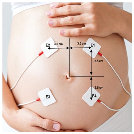
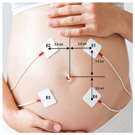
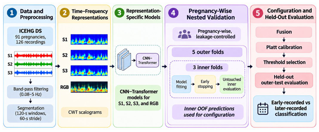
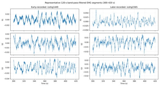
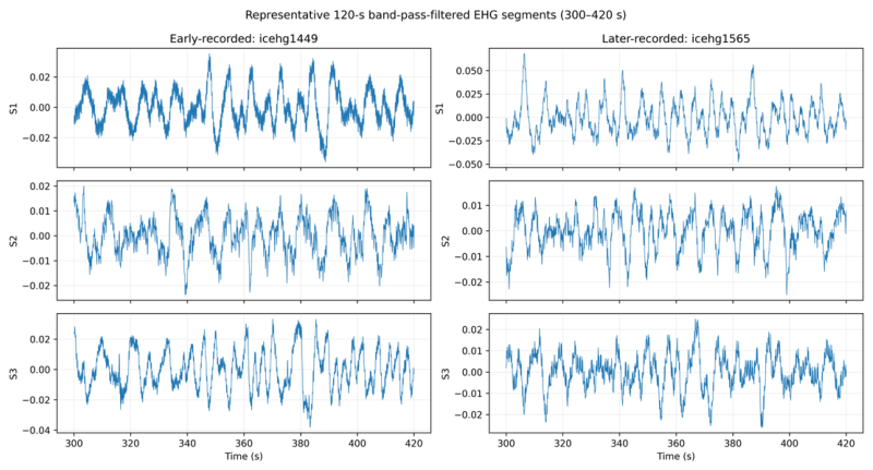
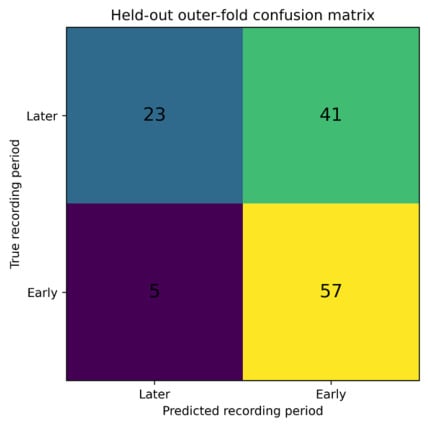
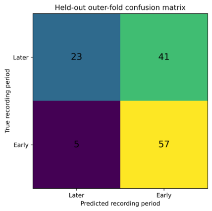
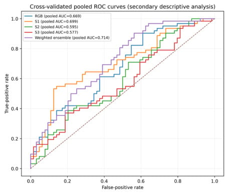
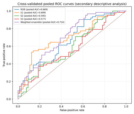
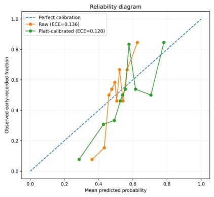
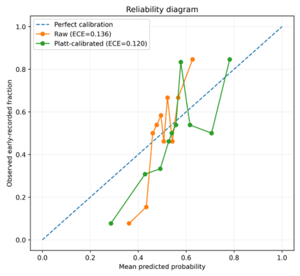
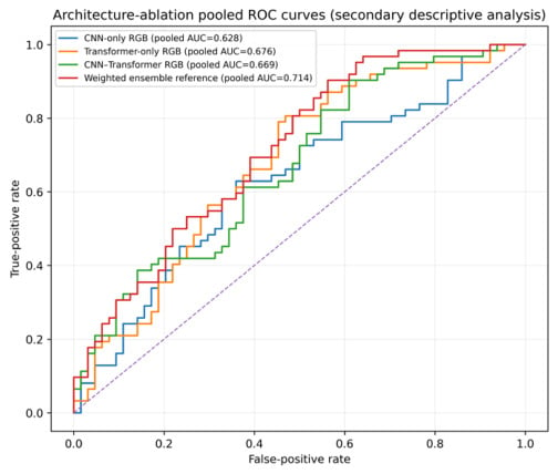
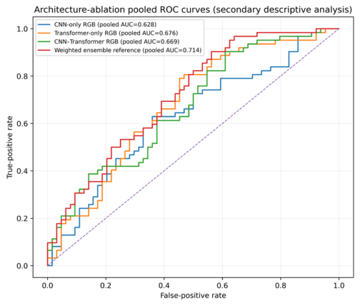
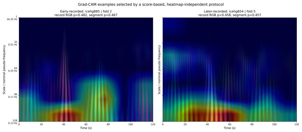

Disclaimer/Publisher’s Note: The statements, opinions and data contained in all publications are solely those of the individual author(s) and contributor(s) and not of MDPI and/or the editor(s). MDPI and/or the editor(s) disclaim responsibility for any injury to people or property resulting from any ideas, methods, instructions or products referred to in the content. |
© 2026 by the authors. Licensee MDPI, Basel, Switzerland. This article is an open access article distributed under the terms and conditions of the Creative Commons Attribution (CC BY) license.