


Abstract
Large basins show substantial variation in the timing and persistence of hydrological responses to climatic forcing. Quantifying hydroclimatic lags and basin memory is important for understanding hydrological response dynamics, assessing drought persistence, and informing future research on drought prediction and water-resource management. This study presents a harmonised comparison of hydroclimatic response delays and hydrological memory across ten major European basins. Basin-scale Water Budgets (WBs) were derived from precipitation, evapotranspiration, and runoff components, while hydroclimatic forcing was represented by the Combined Climatologic Deviation Index (CCDI), based on precipitation anomalies and Gravity Recovery and Climate Experiment (GRACE) total water storage anomalies (TWSAs). Cross-correlation (CCF), autocorrelation (ACF), partial autocorrelation (PACF), and autocorrelation decay time (e-folding) were used to quantify response timing and persistence. The results show basin-specific differences in lag relationships and autocorrelation-based persistence. Estimated memory durations depend on the diagnostic used, highlighting the need to distinguish e-folding time, zero-crossing lag, and significance-decay lag. Because WB and CCDI share precipitation-related information, the observed cross-correlations are interpreted as statistical associations rather than direct evidence of causality. The findings provide a comparative assessment of hydroclimatic lag and persistence characteristics for the selected basins and study period; their predictive value requires separate validation.
1. Introduction
Hydroclimatic response lag describes the temporal offset between variations in an external climatic driver and the associated hydrological response [1,2]. It is commonly quantified using cross-correlation analysis, which identifies the time shift associated with the strongest statistical relationship between two variables. In contrast, hydrological memory refers to the persistence of information from antecedent hydrological conditions within the system. It reflects the extent to which previous states influence subsequent hydrological variability and can be quantified using autocorrelation-based diagnostics, including the autocorrelation function (ACF), partial autocorrelation function (PACF), and characteristic autocorrelation decay time (e-folding time).
Although response lag and hydrological memory may both be influenced by water storage and release processes, they describe different temporal properties. A basin may respond rapidly to changes in climatic conditions while retaining substantial hydrological memory due to slowly varying groundwater, soil moisture, or snow storage. Conversely, a delayed response does not necessarily imply long-lasting persistence. Therefore, response lag is interpreted in this study as the temporal displacement between the analysed hydroclimatic indicators, whereas hydrological memory represents the persistence of their individual temporal anomalies [3].
Previous studies have investigated hydrological memory at multiple spatial scales. Berghuijs [4] demonstrated that annual water-cycle memory varies substantially among climatic regions and is strongly controlled by storage processes. Khanal [3] showed that hydrometeorological memory significantly influences compound flood generation in the Rhine Basin. Rahmati [2] emphasised the dominant role of soil moisture storage in regulating persistence across terrestrial systems. Staudinger [5] further highlighted the importance of groundwater and snow storage in sustaining hydrological droughts.
Despite these advances, most existing studies have focused on individual basins, specific hydrological variables, or local-scale processes. Comparative continental-scale analyses integrating climatic forcing, water-storage anomalies, response lags, and persistence diagnostics within a unified framework remain scarce.
Autocorrelation analyses reveal substantial variability in hydrological memory across European basins. Basins characterised by short Autocorrelation Decay Time (e-folding times) exhibit rapidly decaying autocorrelations (ACF), indicating limited storage capacity and fast system turnover. Conversely, basins with long e-folding times maintain significant autocorrelation over several months, pointing to strong memory effects associated with snowpack, groundwater, or large basin size. Partial autocorrelation (PACF) results suggest that, while short-term persistence dominates in fast-responding basins, longer-term dependencies play a key role in basins with delayed hydroclimatic responses [4]. Additionally, cross-correlation function (CCF) analyses enable the identification of time-lagged relationships between the Combined Climatologic Deviation Index (CCDI) and the Water Budget (WB), providing insight into the timing and strength of basin responses to climatic forcing.
The research aims to assess lag and memory effects in ten major European basins (Boreal/Northern Basins: Neva, Pechora, and Northern Dvina; central European Basins: Rhine, Elbe, Vistula, and Danube; continental Eastern Basins: Volga, Dnieper, Don). The study attempted to determine:
- •
- Which basins show an immediate WB response to changes in CCDI?
- •
- Which basins react with a delay, indicating the presence of hydrological memory?
- •
- Does the nature of the response differ between the winter and summer seasons?
A crucial aspect of this paper, which extends the study of European basins, is the combination of CCF + ACF + PACF + e-folding time with the addition of seasonal analysis, as well as the separation of climatic forcing and hydrological response. Furthermore, the presented analysis includes a spatial analysis of how strongly the basin is dependent.
Despite these advances, previous research has largely focused on individual basins, specific drought events, or single persistence metrics. No previous study has systematically compared hydroclimatic response lags and hydrological memory across the largest European basins using harmonised datasets and a unified analytical framework. Europe provides an ideal natural laboratory because it includes strong climatic gradients ranging from oceanic western regions to continental eastern lowlands and snow-dominated northern basins.
The contribution of this study is a harmonised comparison of hydroclimatic lag relationships and autocorrelation-based persistence diagnostics across ten major European basins. By applying complementary metrics to the same study period, the analysis illustrates how the interpretation of basin persistence depends on the variable and operational definition used. The comparison is intended as a descriptive assessment of the selected basins rather than a validation of a universally applicable continental-scale pattern. While previous studies have typically focused on single basins, individual drought indicators, or one-dimensional persistence metrics, this work integrates CCF, ACF, PACF, and e-folding time within one comparative framework. This combined approach enables simultaneous separation of climatic forcing (for CCDI) and hydrological response (for WB), quantification of response delays, and estimation of persistence timescales. A further innovative aspect is the explicit seasonal decomposition, which reveals contrasting summer and winter memory regimes associated with evapotranspiration control versus snow storage and delayed runoff processes. In addition, the study introduces continental-scale hydrological memory mapping for Europe, demonstrating coherent west-east and south–north gradients in basin inertia. These findings provide a transferable framework for comparative drought assessment and hydrological memory analysis and may inform future research investigating whether persistence characteristics and hydroclimatic lag structures can improve drought prediction and support water-resource management. The novelty of this study extends beyond the application of established statistical tools. To our knowledge, this is the first study to jointly quantify hydroclimatic response lag and hydrological memory across the ten largest European river basins using a harmonised Gravity Recovery and Climate Experiment—Modern-Era Retrospective analysis for Research and Applications (GRACE–MERRA) framework. This approach enables direct comparison of response timing and memory characteristics among basins spanning oceanic, continental, and boreal hydroclimatic regimes. Furthermore, the study introduces the first continental-scale hydrological memory mapping of Europe based on combined persistence diagnostics, providing new insight into how storage processes, climatic gradients, and seasonal controls govern the propagation of hydroclimatic anomalies. The resulting framework is transferable to other large basin systems worldwide.
2. Data Description
The analysis was conducted for the ten largest European basins: Volga, Danube, Dnieper, Don, Northern Dvina, Pechora, Neva, Rhine, Vistula, and Elbe (Figure 1). These basins represent a wide range of hydroclimatic settings, from oceanic western Europe to continental eastern Europe and snow-dominated northern regions, making them suitable for comparative assessment of basin-scale memory processes. Basin polygons were used for spatial averaging of terrestrial water storage anomalies derived from GRACE as well as MERRA-2 variables [6].
Figure 1.
Location of the ten largest European basins analysed in this study: (1) Volga, (2) Danube, (3) Dnieper, (4) Don, (5) Northern Dvina, (6) Pechora, (7) Neva, (8) Rhine, (9) Vistula, and (10) Elbe [6].
To determine two indices necessary for research, Total Water Storage (TWS) was obtained from observations of the GRACE mission and precipitation (P), evapotranspiration (EV), and surface runoff (SRO) from the MERRA-2 Reanalysis model. TWS is the sum of all water resources, i.e., those on the Earth’s surface, in the atmosphere, and underground. Observations have been updated monthly since 2002, thanks to the operation of the GRACE mission. The use of GRACE mission observations in the study of water changes in basins is common. However, due to insufficient spatial resolution, smaller areas cannot be reliably covered by the study [7,8,9]. The mission’s satellites measure very small changes in the Earth’s gravity field, which are used to calculate changes in water mass [10]. Knowledge of the TWS allows for the observation of droughts and water resource recovery on a regional and continental scale [11], reveals long-term trends in groundwater depletion [12], enables the analysis of hydrological memory and deficit accumulation [13], and serves as an independent source of data for validating hydrological and climate models.
Precipitation is water from the atmosphere that reaches the Earth’s surface in the form of rain, snow, hail, or drizzle. It is the primary source of water inflow to terrestrial systems and a fundamental element of the hydrological cycle. It is a key input to the WB, influencing surface and groundwater resources, soil moisture, and the risk of drought and flooding [14,15]. Evapotranspiration is the combined process of water evaporation from soil surfaces and water bodies (evaporation) and plant transpiration. It is responsible for the return of water from land to the atmosphere. It is a major component of water outflow from terrestrial systems to the atmosphere—it controls water availability in the soil, plant productivity, and the local climate [16,17].
The portion of precipitation that does not infiltrate into the soil or evaporate, but rather flows across the land surface into rivers, lakes, and oceans, is surface runoff. It is the primary mechanism for water transport in the landscape, determining river recharge, flood risk, and the availability of water resources [18,19].
For this study, data were acquired from https://grace.jpl.nasa.gov/data/get-data/jpl_global_mascons/, accessed on 5 February 2026 (1° × 1° grid) and https://gmao.gsfc.nasa.gov/gmao-products/merra-2/data-access_merra-2/, accessed on 4 February 2026 (0.5° × 0.625° grid). The research was carried out for the time span April 2002–December 2023. The mean values were computed for every month over every single basin according to Figure 1 in such a way as to strictly cover only the land and avoid the influence of marine areas. Since the study considered entire basin areas—using values averaged over a given month—the varying resolutions of the models employed did not affect the final results. Neither GRACE nor MERRA provides point-based values; the data are inherently interpolated, so there is no need to standardise the data grids when dealing with large basin areas. The MERRA-2 data in kg/m2/s were recomputed to obtain the TWS unit (centimetre). Values of P, EV, and SRO were divided by 10, as 1 kg of water is 1000 cm3, so 1 L, and 1 m2 is 10,000 cm2. Each value was multiplied by the number of seconds in each month to be able to change the flow [kg/m2/s] value to static [cm].
3. Methods
The overall workflow of the study is summarised in Figure 2. Basin-scale hydroclimatic forcing and hydrological response were represented using two complementary indicators: WB and the CCDI.
Figure 2.
Stages of research presented in the paper—flowchart.
The WB was computed based on [12,20]:
WB = P− EV− SRO
The WB formulation used in this study represents a simplified basin-scale water budget based on the dominant atmospheric and surface fluxes available from MERRA-2. Groundwater exchange and interflow are not included as explicit terms because they are not directly provided as independent basin-wide variables in the reanalysis product. Their influence is therefore represented only indirectly through the integrated hydrological response.
Before calculating the hydroclimatic indices and performing the time-series analyses, the monthly time series of all variables were checked for missing observations and temporal discontinuities. The analysis period extended from April 2002 to December 2023. No gap-filling procedure was applied to the analysed time series of MERRA observations. Missing values of TWS observations were handled using linear interpolation.
Then, Climatologic Deviation (CD) is [21,22]:
where PAR: precipitation anomaly residual; TWSAR: total water storage anomaly residual. PA is computed as , where PA—precipitation anomaly time series, P—precipitation time series, and —monthly average precipitation value. Residuals are computed as , where PAR—precipitation anomaly residual time series, and —average precipitation anomaly for a given month. Total water storage anomaly residuals are , where TWSAR—total water storage anomaly residual time series, TWSA—total water storage anomaly time series, and —monthly average total water storage anomaly value. TWSA is computed as .
CD = PAR + TWSAR
And the CCDI is [21,22]:
where : mean value of CD; st.dev.CD: CD standard deviation.
3.1. Lag Response Analysis
Cross-correlation functions (CCFs) CCDI(t) and WB(t+ lag) were calculated between the monthly deseasonalised CCDI and WB time series for lags ranging from −24 to +24 months. For each basin, the dominant lag was identified as the lag at which the absolute cross-correlation coefficient reached its maximum within the predefined lag window. The corresponding signed correlation coefficient was retained to distinguish positive from negative associations. Positive lags indicate that CCDI leads WB, whereas negative lags indicate that WB leads CCDI; a lag of zero indicates a contemporaneous relationship. The selected lag represents the strongest linear association within the analysed window and was interpreted as a statistical response timescale rather than a direct estimate of water travel time [23].
Statistical significance of the cross-correlation coefficients was assessed using the conventional approximate 95% significance limits. Cross-correlation coefficients falling outside these limits were considered statistically significant at the nominal 5% significance level. These limits provide an approximate criterion for evaluating the strength of the cross-correlation at individual lags.
Hydrological lag is traditionally defined as the delay between precipitation forcing and runoff response. In the presented study, the term lag refers more specifically to the statistical delay between climatic anomalies represented by CCDI and hydrological anomalies represented by WB. Therefore, the estimated lag should be interpreted as a hydroclimatic response timescale rather than a direct rainfall-runoff travel time.
3.2. Memory Diagnostics
Hydrological persistence was assessed using three complementary metrics:
- •
- ACF: quantifies dependence between present and past states.
- •
- PACF: isolates direct lag influence after removing intermediate lag effects.
- •
- E-folding time: defined as the lag at which ACF declines below 1/e, representing characteristic memory duration.
Together, these metrics capture both short-term persistence and longer system memory.
For each series, the ACF was calculated for subsequent time lags. The function allows for the assessment of the degree of dependence of values on their previous states and the identification of the time scale of the signal persistence in the system [23,24,25].
The PACF allows for the determination of the direct effect of a given lag after removing the influence of intermediate lags. PACF was used to identify the dominant time scales and the potential order of the autoregressive process describing the variability of the time series [26].
The e-folding time was defined as the lag at which the ACF drops to 1/e of the initial value. This parameter was treated as a measure of the basin’s hydrological memory and was used to compare basins and seasons [2].
Rescaled Range (R/S) analysis is a well-established method for assessing long-range dependence and estimating the Hurst exponent. However, the objective of this study was not to quantify fractal persistence or scaling behaviour but rather to identify physically interpretable response timescales and lag structures. ACF, PACF, and e-folding time were therefore selected because they directly quantify persistence duration, autoregressive structure, and characteristic memory time in units of months, facilitating hydrological interpretation and comparison among basins.
To distinguish different aspects of temporal persistence, hydrological memory was characterised using three separate autocorrelation-based metrics. First, the zero-crossing lag was defined as the first positive lag at which the autocorrelation function (ACF) became negative. Second, the e-folding time was defined as the first lag at which the ACF decreased to or below 1/e. Third, the significance decay lag was defined as the first lag at which the ACF fell below the adopted statistical significance threshold. Each metric was calculated separately for WB and CCDI for every basin. The three metrics were mapped independently and were not averaged or weighted to produce a single memory value. Where a threshold was not reached within the analysed lag window, the metric was treated as right-censored at the end of that window rather than interpreted as an exact memory duration.
3.3. Definition and Interpretation of Hydrological Memory Metrics
To distinguish different aspects of temporal persistence, hydrological memory was characterised using three complementary diagnostics derived from the autocorrelation function (ACF). The first-zero-crossing lag was defined as the smallest positive lag at which the ACF became negative. The e-folding time was defined as the smallest positive lag at which the ACF decreased to or below (1/e) (approximately 0.368). The significance-decay lag was defined as the smallest positive lag at which the ACF fell within the adopted 95% confidence limits around zero. The latter was estimated to use the same significance criterion for all basins and variables.
These metrics quantify different properties of persistence and are therefore not expected to yield identical values. The e-folding time represents the characteristic timescale of autocorrelation decay, the zero-crossing lag identifies the transition from positive to negative autocorrelation, and the significance-decay lag indicates how long autocorrelation remains distinguishable from zero under the selected statistical criterion. If the relevant threshold was not reached within the maximum analysed lag of 60 months, the metric was recorded as not reached within the analysis window rather than interpreted as an exact memory duration of 60 months.
The three metrics were calculated separately for the Water Budget (WB) and the Combined Climatologic Deviation Index (CCDI). They were not treated as interchangeable estimates of a single memory duration.
3.4. Separation of Seasonal Periodicity and Hydrological Persistence
To distinguish seasonal periodicity from inter-monthly hydrological persistence, autocorrelation analysis was performed on the original WB series and on seasonally adjusted series. The monthly climatological mean μm was calculated separately for each calendar month over the study period and subtracted from the corresponding monthly WB observations. This procedure removed the mean annual cycle while preserving temporal anomalies relative to the climatological conditions. Autocorrelation functions (ACFs) were then recalculated for the seasonally adjusted series and compared with those obtained from the original data.
The monthly climatological means were calculated using the entire study period as the reference period. The climatological mean for m month is as follows:
where Xy,m is the value of the variable in month m and year y; Yref a reference period; and Nm is the number of observations in a month.
Seasonality was deleted with
A trend was deleted using
where and are trend parameters computed with the least squares method for time series.
Standardization was conducted using
To assess the potential influence of long-term changes, trends in the WB series were evaluated separately, and autocorrelation was examined after removing the estimated trend. The persistence characteristics derived from the different preprocessing variants were compared in terms of the ACF decay pattern, the presence of peaks at annual multiples, and the resulting e-folding time. This comparison was used to assess the extent to which the estimated persistence reflected the recurring annual cycle, long-term changes, or residual inter-monthly dependence. The interpretation of persistent autocorrelation as evidence of storage-related hydrological memory was restricted to patterns that remained after accounting for seasonal periodicity and trend effects.
3.5. Robustness Analysis of Temporal Persistence and Lag Relationships
To evaluate the sensitivity of estimated persistence and lag relationships to seasonal cycles and long-term trends, the ACF, PACF, CCF, and e-folding diagnostics were compared across alternative preprocessing scenarios. For each monthly series, four variants were considered: the original series, a deseasonalised series obtained by subtracting the climatological mean for each calendar month, a linearly detrended series obtained by removing the fitted linear trend, and a series that was both deseasonalised and detrended. The same preprocessing definitions and analysis windows were applied consistently across basins and variables.
The ACF and PACF were used to describe within-series temporal dependence, while the CCF was used to quantify lagged statistical associations between the analysed variables. For each basin, the lag corresponding to the maximum absolute CCF coefficient was identified, and both the signed correlation coefficient and its associated lag were recorded. The sign of the coefficient was used to describe the direction of the statistical association, whereas the sign of the lag was used to determine the temporal ordering of the two series according to the adopted lag convention. The lag convention was defined explicitly so that positive and negative lags could be interpreted consistently. E-folding times were calculated using the same threshold and search window across preprocessing scenarios. Missing observations were retained at their original monthly positions; correlations were not calculated by simply removing missing months and concatenating the remaining observations.
To examine the potential influence of common meteorological forcing, lag relationships involving independent meteorological variables, including precipitation and potential evapotranspiration where available, were evaluated separately from the WB–CCDI comparison. Because precipitation-related information is shared by WB and CCDI, their cross-correlation alone cannot isolate a causal hydrological response. Results were therefore interpreted as statistical associations. The robustness assessment focused on the consistency of correlation strength, peak lag, ACF/PACF structure, and e-folding estimates across preprocessing scenarios and forcing-variable comparisons.
4. Results
CCF analyses reveal substantial spatial differences in basin response timing across Europe (Figure 3 and Figure 4). Several western and central basins, including the Rhine, Elbe, Danube, and Don, exhibit peak correlations at short lags (0–1 month), indicating rapid adjustment of the WB to hydroclimatic anomalies.
Figure 3.
Cross-correlation function (CCF) between the monthly deseasonalised Combined Climatologic Deviation Index (CCDI) at time t and the Water Budget (WB) at time t + lag for ten major European basins: (a) Volga, (b) Danube, (c) Dnieper, (d) Don, (e) Northern Dvina, (f) Pechora, (g) Neva, (h) Rhine, (i) Vistula, and (j) Elbe. Positive lags indicate that CCDI leads WB, whereas negative lags indicate that WB leads CCDI. The sign of the correlation coefficient indicates whether the two series are positively or negatively associated; it is distinct from the sign of the lag. The lag of the selected CCF extremum identifies the timing of the strongest statistical association within the analysed lag window and does not, by itself, establish causality.
Figure 4.
(a) Heatmap showing the cross-correlation coefficients between the analysed European basins. (b) Dominant lag associated with the maximum absolute cross-correlation for each basin, expressed in months. Positive and negative lag values indicate the temporal ordering defined by the CCF convention used in this study.
In contrast, northern and eastern basins display delayed responses extending over several months. The strongest lagged persistence was identified in the Neva, Pechora, Northern Dvina, and Dnieper systems, suggesting slower propagation of climatic anomalies through storage-dominated hydrological pathways.
These patterns indicate that European basins range from fast-response systems with limited inertia to slow-response systems characterised by substantial storage buffering.
It is assumed that if lag < 0, then WB leads CCDI (i.e., change in WB, and then CCDI); if lag > 0, then CCDI leads WB; and if lag = 0, a synchronous relationship is established.
Cross-correlation analysis revealed differences in the strength and timing of the association between WB and CCDI across the ten analysed basins (Figure 3). For the Neva basin, the maximum positive correlation was approximately 0.33. The corresponding dominant lag should be reported using the lag value confirmed from the underlying CCF results. The lag convention adopted in this study is that a negative lag indicates that WB leads CCDI, whereas a positive lag indicates that CCDI leads WB; a zero lag indicates a contemporaneous association. These lagged correlations describe statistical relationships between the two series and do not, by themselves, demonstrate the physical propagation time of hydroclimatic anomalies. Relatively strong positive correlations were also observed for the Rhine (Figure 3h), Danube (Figure 3b), and Don (Figure 3d), where maximum correlation values exceeded 0.15.
Negative lag values indicate that WB leads CCDI under the lag convention adopted in this study. This temporal ordering may reflect differences in the temporal behaviour of the two indicators. WB integrates precipitation, evapotranspiration, and surface runoff, whereas CCDI combines precipitation anomalies with terrestrial water storage information derived from GRACE. Differences in temporal aggregation, smoothing of GRACE-derived storage signals, and shared variability between the component time series may influence the estimated lag. Because precipitation-related information is present in both indicators, the observed relationship cannot be interpreted as an isolated causal response. Therefore, a negative lag indicates that WB statistically precedes CCDI, but does not establish a causal sequence or identify a unique hydrological mechanism. This interpretation applies regardless of whether the corresponding CCF coefficient is positive or negative.
The CCF heatmap (Figure 4a) shows distinct patterns of association across the analysed basins and lag values. The Neva exhibits the clearest positive correlations, particularly at negative lags. In contrast, the Vistula displays predominantly negative correlations across much of the analysed lag range, with values approaching approximately −0.35 on the heatmap. The Northern Dvina shows a mixture of positive and weaker correlations, while the Volga and Dnieper generally exhibit weaker associations. These patterns demonstrate that the strength and sign of the WB–CCDI association vary between basins and depend on the lag considered. The sign of the correlation coefficient should be distinguished from the sign of the lag, which determines the direction of the temporal relationship under the convention adopted in this study.
The CCF results indicate substantial basin-to-basin variability rather than a uniform continental gradient in the association between WB and CCDI. The Neva shows a relatively strong positive association at negative lags, whereas the Vistula is characterised by predominantly negative correlations. The Northern Dvina and Pechora exhibit more variable patterns across the lag window. These differences may reflect contrasts in the temporal behaviour of the two hydroclimatic series; however, the CCF results alone cannot establish which physical storage or runoff processes are responsible for the observed patterns. The results should therefore be interpreted as basin-specific statistical relationships rather than direct evidence of differences in the physical propagation of hydroclimatic anomalies.
Figure 4a presents the cross-correlation coefficients between CCDI and WB across lags ranging from −24 to +24 months. The heatmap reveals marked differences in both the magnitude and sign of the CCF coefficients among basins and across lag values. The Neva basin exhibits the most prominent band of positive correlations, with the highest values occurring at negative lags of approximately −12 to −4 months. This pattern indicates that the strongest positive statistical associations occur when WB leads CCDI under the lag convention adopted in this study. In contrast, the Vistula basin is characterised by predominantly negative CCF coefficients across the analysed lag range, with the strongest negative values occurring at positive lags. The Northern Dvina and Pechora show more spatially variable patterns across lags, including alternating positive and negative coefficients. The Volga and Dnieper generally exhibit weaker associations than the prominent positive pattern observed for the Neva. Overall, the heatmap demonstrates that the strength, sign, and timing of the WB–CCDI association differ substantially among the analysed basins. These patterns represent statistical relationships and do not, by themselves, establish causal mechanisms. Figure 4b shows the dominant lag associated with the maximum absolute cross-correlation for each analysed basin. The sign of the lag identifies the temporal ordering of the two series according to the convention adopted in this study: negative lags indicate that WB leads CCDI, whereas positive lags indicate that CCDI leads WB. A lag of zero indicates that the strongest association occurs without a temporal offset. Differences in dominant lag among basins demonstrate that the timing of the strongest WB–CCDI association is basin-specific. These lag estimates describe the temporal structure of statistical associations and, by themselves, do not establish causal hydrological response times.
Figure 4b shows substantial differences in the dominant lag associated with the maximum absolute CCF among the ten basins. The largest positive lag occurs in the Dnieper basin, at approximately +23 months, followed by the Northern Dvina at about +13 months. Positive lags are also observed for the Elbe and Vistula, at approximately +9 and +8 months, respectively. In contrast, the largest negative lag occurs in the Pechora basin, at approximately −15 months, while the Neva and Volga exhibit negative lags of about −8 and −7 months. The dominant lags for the Danube, Don, and Rhine are close to zero and slightly negative, indicating that their strongest WB–CCDI associations occur with little temporal offset. According to the adopted lag convention, positive lags indicate that CCDI leads WB, whereas negative lags indicate that WB leads CCDI. The results therefore show that the timing of the strongest association varies considerably among basins, with the Dnieper and Pechora exhibiting particularly large absolute lag values. These values identify the lags of maximum absolute cross-correlation; they should not be interpreted directly as causal hydrological response times.
As a next step, the ACF and the PACF were computed for the whole time series (Figure 5 and Figure 6) and seasonally for summer (April–September) and winter (October–March) (Table 1). ACF diagnostics demonstrate pronounced continental gradients in persistence. Western basins generally show rapid decay of autocorrelation, reflecting dynamic hydrological turnover and stronger direct atmospheric control. By contrast, northern and eastern basins maintain significant positive autocorrelation over extended lags, indicating long-memory behaviour.
Figure 5.
Autocorrelation functions (ACFs) of the monthly WB and CCDI for ten major European basins. For each basin, the left panel shows the WB ACF and the right panel shows the CCDI ACF. The panels are arranged in the following order: (a,b) Volga, (c,d) Danube, (e,f) Dnieper, (g,h) Don, (i,j) Northern Dvina, (k,l) Pechora, (m,n) Neva, (o,p) Rhine, (r,s) Vistula, and (t,u) Elbe. The horizontal axis represents lag in months, and the vertical axis represents the autocorrelation coefficient. A slower decay of the ACF indicates more persistent temporal dependence in the corresponding time series. In all basins, the ACF starts at 1 (lag = 0), then gradually decreases with lag, and the rate of decrease varies spatially (Figure 5). Therefore, it can be concluded that European basins exhibit varying levels of hydroclimatic inertia. The basin with short memory is the Volga (a,b) for the WB and CCDI; the correlation quickly disappears, indicating a rapid response to precipitation forcing. In Rhine and Elbe (o,p,t,u), the WB decreases moderately quickly, but the CCDI maintains correlation longer. Basins with medium memory are the Danube, Don, and Vistula (Figure 5c,d,g,h,r,s), where the WB exhibits clear autocorrelation for several to a dozen months, and the CCDI maintains positive values even longer. In these systems, a coupled climate–hydrology memory is evident. The basins with the longest memories include the Dnieper, Northern Dvina, Pechora, and Neva (e,f,i–n). These basins exhibit a very slow decline in ACF, maintaining positive autocorrelation for long periods and often lacking a rapid transition to values close to zero. The dominance of the continental climate is noticeable here. PACF results indicate that lag-1 dependence dominates in many western and central basins, implying that recent antecedent conditions largely determine current monthly states. In contrast, northern basins exhibit multi-lag structures, suggesting cumulative controls operating over several months.
Figure 6.
Partial autocorrelation functions (PACFs) of monthly Water Budget (WB) and Combined Climatologic Deviation Index (CCDI) for ten major European basins. The panels are arranged in pairs, with WB shown in the left panel and CCDI in the right panel for each basin. The basin pairs are presented in the following order: (a,b) Volga, (c,d) Danube, (e,f) Dnieper, (g,h) Don, (i,j) Northern Dvina, (k,l) Pechora, (m,n) Neva, (o,p) Rhine, (r,s) Vistula, and (t,u) Elbe. The horizontal axis represents lag in months, and the vertical axis represents the partial autocorrelation coefficient. Significant peaks indicate direct lag dependence after accounting for the effects of intermediate lags.
Table 1.
ACF and PACF computed for WB and CCDI in different parts of the year (summer and winter) for ten major European basins.
Based on the PACF WB analysis, a strong peak in lag 1–3 was observed, indicating a short hydrological memory, which is a rapid WB response and the dominance of atmospheric processes. For the PACF CCDI, several significant lags were observed, as well as a slower decay than for the WB.
ACF analysis indicates that most basins are dominated by significant first-order autoregressive dependence. In northern basins such as Neva and Pechora, several additional significant lags are observed beyond lag 1, suggesting that persistence is distributed across multiple timescales. However, the strongest direct influence remains concentrated within the first few months. The PACF results reveal that the lag-1 coefficient is generally larger for CCDI than for WB. For example, CCDI exhibits positive lag-1 coefficients across nearly all basins, whereas WB coefficients vary substantially between seasons and occasionally change sign. This behaviour suggests that drought-related anomalies maintain stronger month-to-month persistence than water-balance fluxes, which are more strongly influenced by seasonal hydrological processes. Seasonal decomposition reveals strong winter enhancement of WB memory, particularly in northern basins. Neva, Pechora, and Northern Dvina display substantially stronger cold-season persistence than summer persistence, consistent with snow accumulation, delayed meltwater release, and frozen-ground storage effects.
Summer memory is generally weaker and often close to zero in western and southern basins, indicating rapid evapotranspiration-driven adjustment. In contrast, CCDI remains comparatively persistent in both seasons, suggesting that drought-related anomalies integrate cumulative forcing beyond direct seasonal controls.
Table 1 indicates that winter persistence of WB is generally higher in northern basins than in summer. The strongest winter ACF values are observed for Neva (0.386) and Pechora (0.172), whereas summer values are close to zero in most basins. In contrast, CCDI exhibits relatively stable positive autocorrelation across seasons, particularly in Dnieper (0.623 summer; 0.559 winter), Elbe (0.502 summer; 0.375 winter), and Vistula (0.480 summer; 0.359 winter). These results suggest that drought-related anomalies preserve memory more consistently throughout the year than monthly water-budget fluxes.
The last part of the research was to calculate the e-folding for WB and CCDI (Figure 7). E-folding diagnostics confirm shorter characteristic memory for WB than for CCDI in most basins. WB memory typically ranges from 1 to 3 months in fast-response systems, whereas CCDI persistence commonly extends beyond 6 months and reaches substantially longer timescales in continental basins.
Figure 7.
E-folding times of monthly (a) Water Budget (WB) and (b) Combined Climatologic Deviation Index (CCDI) series for the ten analysed European basins. E-folding time is defined as the first positive lag at which the ACF decreases to or below (1/e) (approximately 0.368). Values are expressed in months. The estimates describe the characteristic decay timescale of autocorrelation and should not be interpreted as equivalent to the zero-crossing or significance-decay lag.
This consistent difference indicates that drought indices preserve hydroclimatic anomalies longer than monthly water-budget fluxes.
The e-folding estimates generally indicate shorter autocorrelation decay times for WB than for CCDI. However, the magnitude of this difference varies among basins and depends on the preprocessing applied to the time series. In particular, the long e-folding times obtained for the Dnieper, Elbe, and Don in the original series decrease substantially after deseasonalisation and detrending. These results indicate that part of the apparent long-term persistence is associated with seasonal or low-frequency variability. The e-folding estimates should therefore be interpreted together with the robustness analysis rather than as invariant measures of basin memory.
Based on the research carried out, an analysis of the hydrological memory of the largest European basins was prepared (Figure 8). Three elements were considered to generate the memory maps:
Figure 8.
Spatial distributions of three complementary hydrological persistence metrics across the analysed European river basins: (a) e-folding time, (b) first zero-crossing lag, and (c) significance-decay lag. All metrics are expressed in months but represent different aspects of autocorrelation persistence. Values that were not reached within the 60-month analysis window are identified separately and are not interpreted as exact durations of 60 months.
- •
- First lag, where ACF < 0;
- •
- e-folding time (ACF = 1/e);
- •
- Lag, where ACF falls below statistical significance.
Figure 8 presents complementary measures of hydrological persistence across the analysed European river basins. The e-folding time, first zero-crossing lag, and significance-decay lag characterise different aspects of autocorrelation behaviour and should therefore be interpreted separately rather than treated as interchangeable estimates of a single memory duration.
The e-folding time describes the rate at which autocorrelation decreases to approximately 1/e of its initial value, whereas the first zero-crossing lag identifies when autocorrelation first becomes negative. The significance-decay lag indicates the timescale at which autocorrelation no longer remains statistically significant under the criterion adopted in this study. Differences between these measures are therefore expected because they represent distinct properties of temporal persistence.
An important consideration is the 60-month analysis window. When a threshold is not reached within this interval, the corresponding persistence duration cannot be determined precisely from the available analysis. Such cases should be reported as exceeding the analysed window or as not reached, according to the notation used in the figure, rather than interpreted as exact durations of 60 months.
The Hydrological Memory Map (WB-CCDI) shows the memory difference calculated as follows:
WB − CCDI = Memory difference
Equation (8) compares memory metrics expressed in identical units (months). Therefore, the subtraction is mathematically valid and represents the difference in persistence duration between WB and CCDI rather than a difference between the original variables themselves.
Negative values (WB < CCDI) dominate in most basins, meaning the CCDI index demonstrates a longer memory than the actual WB. The difference in Central Europe (Rhine, Elbe, and Vistula) is smaller. In more oceanic regions, the hydrological system responds more quickly, and the CCDI better reflects the actual dynamics of WB. The difference between WB and CCDI memory indicates that the climatic drought index generally exhibits longer persistence than the physical WB, particularly in northern and eastern Europe. This suggests that CCDI integrates hydroclimatic signals over longer timescales than the actual water storage dynamics.
Taken together, the results demonstrate a robust continental-scale gradient of hydrological memory across Europe:
- •
- Shorter memory in oceanic and temperate western basins;
- •
- Intermediate persistence in central Europe;
- •
- Very long memory in continental and boreal northeastern basins.
This gradient reflects differences in climatic regime, snow dominance, groundwater storage capacity, and basin scale. The results indicate that hydroclimatic anomalies propagate and persist for substantially longer periods in northern and eastern Europe than in western and central regions.
Robustness of Lag and Persistence Estimates
The robustness analysis indicates that the estimated persistence timescales and hydroclimatic response lags depend on both the variable analysed and the preprocessing procedure (Table 2). For WB, e-folding times were generally short, ranging from 1 to 3 months in the raw series and from 1 to 2 months after deseasonalisation and detrending. The Vistula exhibited the longest WB e-folding time in the raw data (3 months), which decreased to 1 month after both seasonal and linear-trend components were removed. This reduction indicates that part of the apparent persistence in the original WB series may be associated with seasonal variability or low-frequency trend components.
Table 2.
Robustness of e-folding times and CCF lag estimates.
CCDI showed substantially longer persistence than WB in most basins. In the raw series, the estimated e-folding time reached 48 months in the Dnieper, 40 months in the Elbe, and 30 months in the Don. After removing both seasonality and the linear trend, these estimates decreased to 11, 8, and 12 months, respectively. The largest reductions therefore occurred in the Dnieper and Elbe, suggesting that their long persistence estimates are sensitive to low-frequency variability. In contrast, the Neva retained an e-folding time of 8 months across all four preprocessing variants, while the Pechora remained at 6 months. These results suggest that the persistence estimates for the Neva and Pechora are less sensitive to the tested transformations than those for several continental basins.
The CCF analysis also revealed differences in the stability of estimated response lags. The dominant lag remained at −1 month across all preprocessing variants in the Danube, Don, and Rhine. In the Volga, the dominant lag remained at −7 months. In contrast, the dominant lag changed from 9 to −1 months in the Dnieper after detrending, from 12 to 3 months in the Northern Dvina after deseasonalisation, and from 9 to −1 months in the Elbe after removal of seasonality. The Vistula also showed a change in the dominant lag, from 8 months in the raw series to 1 month in the deseasonalised series. These changes indicate that the estimated timing of the CCDI–WB relationship is not equally robust across the ten basins.
The PACF results provide additional evidence of preprocessing sensitivity. For WB, the lag-1 PACF decreased substantially after deseasonalisation in the Volga (from 0.650 to 0.076), Danube (from 0.425 to 0.086), Dnieper (from 0.525 to approximately zero), and Elbe (from 0.544 to 0.032). This suggests that a considerable part of the short-term dependence in these raw WB series is associated with seasonal structure. By comparison, CCDI retained relatively high lag-1 PACF values after deseasonalisation, including 0.879 in the Volga, 0.920 in the Danube, and 0.956 in the Dnieper. However, these values decreased after detrending, indicating that the persistence of CCDI is also partly influenced by low-frequency variability.
Overall, the robustness tests show that the short e-folding times of WB are comparatively stable, whereas CCDI persistence estimates and selected CCF lags are more sensitive to preprocessing in several basins. The results therefore support interpreting hydrological memory as a metric-dependent property rather than a single, invariant basin characteristic. Nevertheless, these tests assess sensitivity to preprocessing only. Because independent meteorological forcing series were not available in the analysed dataset, they do not establish whether the observed CCDI–WB correlations are independent of shared meteorological drivers. Further testing using separate precipitation and potential evapotranspiration series is required to address this issue.
Table 2 demonstrates that the robustness of the estimated hydrological memory and response lags differs between WB and CCDI and among the analysed basins. The e-folding times for WB are generally short and relatively stable, decreasing from 1–3 months in the raw series to 1–2 months after deseasonalisation and detrending. The reduction observed in the Vistula basin, from 3 months in the raw series to 1 month after both transformations, indicates that part of the apparent persistence in the original WB series was associated with seasonal variability and/or a low-frequency trend.
In contrast, CCDI generally exhibits longer persistence, but its estimated duration is more sensitive to preprocessing in several basins. The most pronounced changes occur in the Dnieper, Elbe, and Don, where the raw-series e-folding times of 48, 40, and 30 months decrease to 11, 8, and 12 months, respectively, after deseasonalisation and detrending. This reduction indicates that the long persistence initially observed in these basins cannot be attributed exclusively to sustained hydroclimatic memory; it is also influenced by seasonal and low-frequency components. Conversely, the e-folding times remain unchanged for the Neva (8 months) and Pechora (6 months) across the tested preprocessing variants, suggesting greater stability of these estimates with respect to the applied transformations.
The dominant CCF lags also show basin-dependent sensitivity to preprocessing. The lag remains at −1 month for the Danube, Don, and Rhine and at −7 months for the Volga across all tested variants, whereas larger changes occur in the Dnieper, Northern Dvina, Elbe, and Vistula. These shifts indicate that the estimated timing of the CCDI–WB relationship may partly depend on seasonal and trend-related variability in the original series. Consequently, response lags should be interpreted with particular caution in basins where their magnitude or sign changes after preprocessing.
Table 3 shows that the stability of the dominant cross-correlation function (CCF) lag and the corresponding correlation coefficient vary among the analysed basins and depend on the preprocessing applied to the time series. The most stable lag estimates were obtained for the Danube, Don, and Rhine, for which the dominant lag remained at −1 month across all four preprocessing variants. In the Volga, the dominant lag was consistently −7 months. These results indicate that the estimated timing of the WB–CCDI relationship in these basins is comparatively insensitive to the removal of seasonal and trend components, although the correlation coefficients vary with preprocessing.
Table 3.
CCF lag and correlation comparison.
In other basins, the dominant lag was more sensitive to preprocessing. In the Dnieper, the lag changed from 9 months in the raw and deseasonalised series to −1 month after detrending. In the Northern Dvina, it decreased from 12 to 3 months after deseasonalisation. In the Elbe, the lag changed from 9 months in the raw series to −1 month after deseasonalisation, while in the Vistula, it changed from 8 months to 1 month. The Pechora and Neva also showed variations in the estimated lag across preprocessing variants. These shifts suggest that seasonal and long-term variability can influence the apparent timing of the relationship between WB and CCDI.
The correlation coefficients provide additional information about the strength and direction of the relationships. In the Danube, the correlation increased from 0.152 in the raw series to 0.296 after deseasonalisation and detrending. A similar increase occurred in the Don, from 0.066 to 0.197. In the Dnieper and Elbe, the correlations changed from negative values in the raw series to positive values after detrending or deseasonalisation, respectively. These changes indicate that the estimated association is sensitive to the temporal structure of the series and should therefore be interpreted in the context of the preprocessing applied.
The Vistula showed a different pattern: its correlation remained negative across all four variants, although its magnitude decreased from −0.361 in the raw series to −0.233 after deseasonalisation and detrending. In contrast, the Rhine exhibited positive correlation coefficients across all four variants, including after deseasonalisation and detrending. This consistency in the sign of the correlation, together with the stable dominant lag of −1 month, indicates that the direction and timing of the WB–CCDI association in the Rhine are more robust to preprocessing than in basins where the correlation changes sign.
5. Discussion
The results demonstrate that hydrological memory is a fundamental property governing large-scale basin behaviour across Europe. Although response lag and memory are related characteristics, they describe different aspects of hydrological functioning. Response lag reflects the characteristic timescale required for climatic anomalies represented by CCDI to be reflected in basin-scale water-balance dynamics, whereas memory describes the persistence of antecedent conditions and the duration over which past states continue to influence present hydrological behaviour. This distinction is consistent with contemporary definitions of hydrological memory proposed by [1,2,4], who emphasise that memory reflects the persistence of storage states rather than the timing of individual hydrological responses.
A pronounced continental gradient was identified across all applied diagnostics. Cross-correlation analysis revealed that most basins exhibited negative lag values, indicating that changes in WB generally preceded corresponding CCDI anomalies. The strongest relationship was observed in the Neva basin, where the maximum correlation reached r = 0.33 at lag = −6 months. In contrast, several central and western European basins displayed considerably shorter response times, indicating more rapid adjustment of hydrological conditions to climatic forcing.
The persistence diagnostics consistently indicated stronger memory in northern and eastern Europe than in western Europe. The longest e-folding memory times were observed in Neva, Pechora, Northern Dvina, and Dnieper, whereas Rhine and Elbe displayed substantially shorter persistence. This spatial pattern is consistent with large storage capacities, seasonal snow accumulation, delayed snowmelt release, and stronger groundwater buffering typical of continental and boreal environments. Berghuijs [4] demonstrated that annual water-cycle memory increases with storage capacity and climatic persistence, whereas Rahmati et al. [2] identified soil-moisture storage as one of the dominant controls regulating terrestrial memory. The longer persistence observed in Neva, Pechora, and Northern Dvina is therefore consistent with previous large-scale assessments of storage-controlled hydrological systems.
The seasonal diagnostics indicate that the estimated persistence differs between summer and winter in several basins, particularly for WB in the northern basins. The pattern is consistent with a possible influence of snow accumulation, frozen-ground conditions, and delayed meltwater release. However, the seasonal autocorrelation coefficients alone do not identify the physical mechanisms responsible for these differences. The results should therefore be interpreted as evidence of seasonal variation in temporal dependence rather than direct proof of specific storage processes. For example, Neva exhibited winter ACF = 0.386 compared with summer ACF = −0.035, while Pechora showed winter ACF = 0.172 compared with summer ACF = 0.004. The role of snow accumulation and delayed meltwater release in sustaining hydrological persistence has been highlighted by Staudinger [5], who showed that snow storage substantially contributes to drought propagation and delayed recovery in cold-climate basins. Similar seasonal controls were also reported by Orth and Seneviratne [27] in analyses of terrestrial water-storage memory.
A clear distinction was observed between WB and CCDI persistence. In most basins, CCDI exhibited substantially higher autocorrelation and longer memory than WB. For example, CCDI autocorrelation reached 0.623 in summer and 0.559 in winter for Dnieper, while corresponding WB persistence was markedly lower. Similar behaviour was observed for Elbe and Vistula. This divergence reflects the different physical meanings of the two variables. WB represents a flux-based quantity responding directly to current hydroclimatic forcing, whereas CCDI integrates precipitation anomalies and storage deficits accumulated over longer periods. Consequently, CCDI retains information from antecedent conditions for longer timescales than monthly water-balance dynamics. Comparable differences between hydrological and meteorological drought persistence have been reported in GRACE-based drought studies. Sinha [21] demonstrated that storage-based drought indicators preserve hydroclimatic information for substantially longer periods than precipitation anomalies alone. Similarly, Ren [13] found that hydrological droughts derived from total water storage anomalies tend to be more persistent and spatially coherent than meteorological droughts.
PACF analysis indicated that direct autoregressive dependence is generally concentrated within the first lag for both variables. However, northern basins occasionally exhibited additional significant lags, suggesting more complex storage-related controls. The stronger and more stable lag-1 dependence observed for CCDI further supports the interpretation that drought development and recovery involve cumulative processes operating over multiple months. This behaviour is consistent with the interpretation of persistence mechanisms proposed by Ding and Zhou [26], who showed that significant low-order partial autocorrelation often reflects direct memory effects, whereas higher-order persistence is commonly associated with storage-mediated processes.
Quantitative comparison with previous studies provides further context for the hydrological memory patterns identified in this study. De Lavenne [28], analysing 685 basins in France and Sweden, found significant multi-year memory in only a subset of catchments, while the characteristic memory duration in catchments exhibiting significant multi-year persistence was commonly 2–3 years in France and less than 2 years in Sweden. These findings demonstrate that memory extending beyond the seasonal timescale occurs in European basins, although its duration varies regionally and depends on basin characteristics. In the present study, the e-folding time of WB was generally short (approximately 1–3 months), whereas CCDI exhibited substantially longer persistence, with the shortest characteristic timescale being approximately 6 months and particularly persistent behaviour identified in the Dnieper, Elbe, and Don basins. The persistence exceeding 60 months identified by some CCDI series further indicates that long-term hydroclimatic variability can remain statistically detectable over several years. However, these values should not be interpreted as directly equivalent to the multi-year memory durations reported by de Lavenne et al. [28] because the studies use different variables and methods to quantify memory.
Independent evidence for differences in hydrological memory among European basins is provided by Sutanto and Van Lanen [29], who reported baseflow index (BFI) values of 0.78 for the Danube and 0.74 for the Rhine, indicating a substantial contribution of baseflow to river discharge in these basins. Their results linked higher BFI and slower groundwater release to greater catchment memory and improved hydrological drought forecast performance. Although BFI is not directly comparable with the e-folding time used here, these findings support the interpretation that storage and delayed groundwater release contribute to hydrological persistence in European basins. Similarly, Orth and Seneviratne [27], using more than 100 near-natural European basins, demonstrated that soil-moisture memory influences the persistence of streamflow and evapotranspiration, with the resulting memory depending on the coupling between soil moisture and these fluxes. Taken together, these studies support the interpretation that hydrological memory varies across Europe and reflects differences in storage, catchment response, and hydroclimatic controls. The distinction observed here between the relatively short memory of WB and the longer persistence of CCDI is therefore consistent with the broader literature, while the harmonised comparison of these two variables across the ten largest European basins provides a complementary perspective on basin-scale hydroclimatic persistence.
The identified persistence patterns may be relevant to future drought-prediction research and water-resource management. In basins with longer estimated persistence, current conditions retain statistical dependence on previous months, which may help researchers select candidate predictors and investigate suitable forecasting horizons. However, the present study does not establish that these characteristics improve predictive performance. No prediction model, out-of-sample validation, or predictive-skill assessment was performed. The results should therefore be interpreted as diagnostic information that may inform future predictive modelling, rather than as evidence of demonstrated forecasting skill or operational early-warning capability. Future work should evaluate the predictive value of these persistence metrics using independent validation data and appropriate performance measures [27,30]. Several limitations should be acknowledged when interpreting the results. GRACE observations provide robust estimates of large-scale total water storage changes but may smooth local hydrological variability due to their effective spatial resolution. These limitations have been discussed extensively by Castellazzi [31] and Humphrey [32] , who highlighted the effects of spatial smoothing, leakage errors, and reduced sensitivity to local groundwater variability in GRACE-derived storage estimates. MERRA-2 water-budget components additionally contain uncertainties associated with model parameterisation and observational constraints. Furthermore, anthropogenic influences such as reservoir operations, groundwater abstraction, irrigation return flows, and inter-basin transfers were not explicitly represented in the WB formulation. These processes may either increase or decrease apparent memory and alter response timing independently of climatic forcing. Consequently, the estimated lag and persistence metrics should be interpreted as dominant basin-scale statistical characteristics rather than invariant physical constants. Despite these limitations, the consistency observed among CCF, ACF, PACF and e-folding diagnostics indicates that the identified continental-scale patterns are robust and physically meaningful.
The WB formulation used here assumes that the dominant basin-scale fluxes are represented by P-EV-SRO [33] . However, groundwater abstractions, reservoir operations, inter-basin transfers, irrigation return flows, glacier melt contributions, and other anthropogenic interventions may substantially modify real storage dynamics. Correlation-based lag diagnostics implicitly assume quasi-stationary and approximately linear relationships, whereas hydrological systems often exhibit nonlinear responses, threshold effects, and regime shifts under prolonged droughts or extreme flood events. Consequently, estimated memory timescales should be interpreted as dominant statistical characteristics rather than invariant physical constants. The framework may therefore perform less reliably in strongly regulated basins, rapidly changing climatic regimes, or basins where episodic extremes dominate annual variability. Despite these limitations, the harmonised multi-basin design remains valuable for identifying first-order continental patterns and relative contrasts in hydroclimatic memory across Europe.
GRACE and MERRA-2 are subject to different sources of uncertainty because they rely on fundamentally different approaches to observing and representing the terrestrial water cycle. The main uncertainty sources in GRACE include measurement noise, residual errors associated with gravity-field processing, signal attenuation caused by spatial filtering and regularisation, and leakage of signals across basin boundaries. These effects may reduce the amplitude of the retrieved TWS anomalies and introduce contributions from neighbouring areas [34]. In contrast, MERRA-2 is a model-assisted atmospheric reanalysis that provides land-surface hydrological variables. Its uncertainties arise from errors in meteorological forcing, including precipitation, the data assimilation system, land-surface model parameterisations, and the representation of hydrological processes. Although observation-based precipitation corrections improve the representation of land-surface hydrology, they do not eliminate errors in precipitation, evapotranspiration, or runoff [35]. The difference in spatial resolution may affect basin-averaged estimates through spatial smoothing, unequal representation of land areas at basin boundaries, and differences in the representation of spatially heterogeneous hydrological signals. The coarser effective resolution of GRACE may attenuate localised storage anomalies and mix signals originating inside and outside a basin. MERRA-2 resolves spatial variability at a finer nominal grid spacing, but its estimates remain subject to model and forcing uncertainties and should not be interpreted as error-free at the grid-cell scale. These representativeness effects are potentially more important for smaller or elongated basins and for regions with strong spatial gradients in water storage. Moreover, the spatial correlation between neighbouring GRACE grid cells means that their errors cannot be assumed to be independent when calculating basin averages.
In the present study, GRACE TWS anomalies are compared with a water-budget series derived from MERRA-2 precipitation, evapotranspiration, and surface runoff. These quantities represent complementary aspects of the terrestrial water cycle and are not expected to be numerically identical. Consequently, differences between them may reflect both genuine differences between storage changes and water budget fluxes and uncertainties associated with the datasets, their spatial support, and their aggregation to basin scale. Basin averaging reduces some local representativeness errors but does not eliminate GRACE leakage, correlated errors, or MERRA-2 model uncertainties. The results should therefore be interpreted in terms of basin-scale hydroclimatic variability and temporal relationships rather than as a direct validation of one dataset against the other.
6. Conclusions
This study provides a harmonised comparison of hydroclimatic response lags and hydrological memory across the ten largest European basins using GRACE-derived storage information and reanalysis-based water-budget components. The results demonstrate that response timing and persistence are related but fundamentally distinct properties of large-scale hydrological systems.
The main conclusions are as follows:
- •
- Western and central European basins generally exhibit shorter response times, whereas several northern and eastern basins show more persistent dynamics and delayed adjustment. These differences highlight the importance of basin-specific characteristics when interpreting relationships between climatic forcing and water-budget variability.
- •
- Hydrological memory exhibits a marked spatial gradient—longer persistence is generally observed in northern and eastern basins, including Neva, Pechora, Northern Dvina, and Dnieper, while Rhine and Elbe show comparatively shorter memory. This pattern is consistent with the influence of climatic conditions and storage processes on the persistence of hydroclimatic anomalies.
- •
- CCDI generally exhibits longer persistence than the monthly water budget. The contrast between the two series indicates that hydroclimatic anomalies may remain persistent beyond the timescale of changes in monthly basin water-budget fluxes. Seasonal analysis further shows enhanced winter persistence in snow-influenced northern basins, consistent with snow accumulation and delayed meltwater release, whereas summer water-budget dynamics are generally more responsive to evapotranspiration.
- •
- The combined analytical framework provides complementary measures of response and persistence. CCF characterises the timing and strength of relationships between CCDI and the water budget, while ACF, PACF, and e-folding diagnostics describe temporal persistence at different levels. Their joint application supports systematic comparison of hydroclimatic behaviour among large basins with contrasting climatic and hydrological regimes.
Overall, the results highlight hydrological memory as a key organising property of European basin behaviour. The identified persistence patterns and hydroclimatic lag structures may inform future drought prediction research, climate adaptation planning, and large-scale water-resource management. However, their value for operational forecasting and early warning remains to be established through predictive modelling and independent skill assessment.
The proposed framework can support European drought monitoring and forecasting by identifying basin-specific response times and persistence characteristics that may help interpret the development and continuation of hydrological deficits. In operational practice, these diagnostics could complement existing drought indicators by helping practitioners distinguish basins where anomalies tend to dissipate relatively quickly from those where deficits may persist across several months or seasons. Seasonal memory patterns may also help guide the timing of preparedness measures in snow-influenced basins. However, operational implementation would require integration with real-time observations and basin-specific information on water demand and management; the present framework is a diagnostic and comparative tool rather than a standalone forecasting system.
Author Contributions
Conceptualization, M.B.; methodology, M.B.; software, M.B. and W.B.-B.; validation, M.B. and W.B.-B.; formal analysis, M.B.; investigation, M.B.; resources, M.B. and W.B.-B.; data curation, M.B.; writing—original draft preparation, M.B.; writing—review and editing, W.B.-B.; visualization, M.B. and W.B.-B.; supervision, W.B.-B. All authors have read and agreed to the published version of the manuscript.
Funding
This research received no external funding.
Institutional Review Board Statement
Not applicable.
Informed Consent Statement
Not applicable.
Data Availability Statement
The raw data supporting the conclusions of this article will be made available by the authors on request. Data concerning GRACE observations were acquired from https://grace.jpl.nasa.gov/data/get-data/jpl_global_mascons/ (accessed on 8 March 2026). Data concerning MERRA observations were acquired from https://gmao.gsfc.nasa.gov/gmao-products/merra-2/data-access_merra-2/ (accessed on 9 April 2026).
Conflicts of Interest
The authors declare no conflicts of interest.
Abbreviations
The following abbreviations are used in this manuscript:
| WB | Water Budget |
| CCDI | Combined Climatological Deviation Index |
| CD | Climatologic Deviation |
| GRACE | Gravity Recovery and Climate Experiment |
| GRACE FO | Gravity Recovery and Climate Experiment Follow-On |
| TWS | Total Water Storage |
| MERRA-2 | Modern-Era Retrospective Analysis for Research and Applications, version 2 |
| P | Precipitation |
| EV | Evapotranspiration |
| SRO | Surface Runoff |
| CCF | Cross-Correlation Function |
| ACF | Auto-Correlation Function |
| PACF | Partial Auto-Correlation Function |
| TWSA | Total Water Storage Anomaly |
| BFI | Baseflow Index |
| R/S | Rescaled Range |
References
- Koutsoyiannis, D. Hydrologic Persistence and The Hurst Phenomenon. In Water Encycl; Lehr, J.H., Keeley, J., Eds.; Surface and Agricultural Water; Wiley: New York, NY, USA, 2005; Volume 4. [Google Scholar] [CrossRef] [Scilit]
- Rahmati, M.; Amelung, W.; Brogi, C.; Dari, J.; Flammini, A.; Bogena, H.; Brocca, L.; Chen, H.; Groh, J.; Koster, R.D.; et al. Soil Moisture Memory: State-of-the-Art and the Way Forward. Rev. Geophys. 2024, 62, e2023RG000828. [Google Scholar] [CrossRef] [Scilit]
- Khanal, S.; Lutz, A.F.; Immerzeel, W.W.; Vries, H.D.; Wanders, N.; Hurk, B.V.D. The Impact of Meteorological and Hydrological Memory on Compound Peak Flows in the Rhine River Basin. Atmosphere 2019, 10, 171. [Google Scholar] [CrossRef] [Scilit]
- Berghuijs, W.R.; Woods, R.A.; Anderson, B.J.; Hemshorn de Sánchez, A.L.; Hrachowitz, M. Annual memory in the terrestrial water cycle. Hydrol. Earth Syst. Sci. 2025, 29, 1319–1333. [Google Scholar] [CrossRef] [Scilit]
- Tallaksen, L.K.; Van Lanen, H.A.J.; Hannaford, J.; Hisda, H.; Kingston, D.G.; Laaha, G.; Prudhomme, C.; Stagge, J.H.; Stahl, K.; an Loon, A.F.; et al. Hydrological drought: Processes and estimation methods for streamflow and groundwater. In Proceedings of the EGU General Assembly 2024, Vienna, Austria, 14–19 April 2024. [Google Scholar] [CrossRef] [Scilit]
- Birylo, M. Multi-Indicator Assessment of Hydrological Change Across Europe Using Satellite Observations. Water 2026, 18, 986. [Google Scholar] [CrossRef] [Scilit]
- Kalu, I.; Ndehedehe, C.E.; Ferreira, V.G.; Janardhanan, S.; Currell, M.; Kennard, M.J. Statistical downscaling of GRACE terrestrial water storage changes based on the Australian Water Outlook model. Sci. Rep. 2024, 14, 10113. [Google Scholar] [CrossRef] [Scilit] [PubMed]
- Liu, X.; Yang, K.; Ferreira, V.G.; Bai, P. Hydrologic model calibration with remote sensing data products in global large basins. Water Resour. Res. 2022, 58, e2022WR032929. [Google Scholar] [CrossRef] [Scilit]
- Thomas, B.F.; Famiglietti, J.S. Identifying climate-induced groundwater depletion in GRACE observations. Sci. Rep. 2019, 9, 4124. [Google Scholar] [CrossRef] [Scilit] [PubMed]
- Richter, H.M.P.; Lück, C.; Klos, A.; Sideris, M.G.; Rangelova, E.; Kusche, J. Reconstructing GRACE-type time-variable gravity from the Swarm satellites. Sci. Rep. 2021, 11, 1117. [Google Scholar] [CrossRef] [Scilit] [PubMed]
- Zhou, J.; Cui, L.; Yao, C.; Meng, J.; Zou, Z.; Lu, Y. GRACE/GFO and Swarm Observation Analysis of the 2023–2024 Extreme Drought in the Amazon River Basin. Remote Sens. 2025, 17, 2765. [Google Scholar] [CrossRef] [Scilit]
- Błaszczak-Bąk, W.; Birylo, M. Study of the Impact of Landforms on the Groundwater Level Based on the Integration of Airborne Laser Scanning and Hydrological Data. Remote Sens. 2024, 16, 3102. [Google Scholar] [CrossRef] [Scilit]
- Ren, C.; Zhang, X.; Tian, J.; Li, X.; Wang, S.; Tang, Z.; Wang, X.; Zhang, Y. GRACE-based hydrological droughts are less frequent but more severe than meteorological droughts in global major basins. J. Hydrol. 2026, 664, 134582. [Google Scholar] [CrossRef] [Scilit]
- Trenberth, K.E.; Smith, L.; Qian, T.; Dai, A.; Fasullo, J. Estimates of the Global Water Budget and Its Annual Cycle Using Observational and Model Data. J. Hydrometeorol. 2007, 8, 1102–1121. [Google Scholar] [CrossRef] [Scilit]
- Kidd, C.; Huffman, G. Global precipitation measurement. Meteorol. Appl. 2011, 18, 334–353. [Google Scholar] [CrossRef] [Scilit]
- Wang, K.; Dickinson, R. A review of global terrestrial evapotranspiration: Observation, modeling, climatology, and climate variability. Rev. Geophys. 2012, 50, RG2005. [Google Scholar] [CrossRef] [Scilit]
- Fisher, J.B.; Melton, F.; Middleton, E.; Hain, C.; Anderson, M.; Allen, R.; McCabe, M.F.; Hook, S.; Baldocchi, D.; Townsend, P.A.; et al. The future of evapotranspiration: Global requirements for ecosystem functioning, carbon and climate feedbacks, agricultural management, and water resources. Water Resour. Res. 2017, 53, 2618–2626. [Google Scholar] [CrossRef] [Scilit]
- Dingman, S.L. Physical Hydrology; Waveland Press: Long Grove, IL, USA, 2015. [Google Scholar]
- Oki, T.; Kanae, S. Global hydrological cycles and world water resources. Science 2016, 313, 1068–1072. [Google Scholar] [CrossRef] [Scilit] [PubMed]
- Birylo, M. Non-Stationarity of Hydroclimatic Memory—Is Hydrological Memory Changing Under Climate Warming? Water 2026, 18, 869. [Google Scholar] [CrossRef] [Scilit]
- Sinha, D.; Sayed, T.H.; Reager, J. Utilizing combined deviation of precipitation and GRACE based terrestrial water storage as a metric for drought characterization: A case study over major Indian river basin. J. Hydrol. 2019, 572, 294–307. [Google Scholar] [CrossRef] [Scilit]
- Nigatu, Z.M.; Fan, D.; You, W.; Melesse, A.M. Hydroclimatic Extremes Evaluation Using GRACE/GRACE-FO and Multidecadal Climatic Variables over the Nile River Basin. Remote Sens. 2021, 13, 651. [Google Scholar] [CrossRef] [Scilit]
- Lo Russo, S.; Suozzi, E.; Gizzi, M.; Taddia, G. A semi-automatic tool for spring-monitoring data analysis and aquifer characterisation. Environ. Earth Sci. 2021, 80, 710. [Google Scholar] [CrossRef] [Scilit]
- Dondurur, D. Chapter 4-Fundamentals of Data Processing. In Acquisition and Processing of Marine Seismic Data; Elsevier: Amsterdam, The Netherlands, 2018; pp. 211–239. [Google Scholar] [CrossRef] [Scilit]
- Liu, Z.; Li, X.; Hu, Z.; Cao, R.; Han, Y.; Wu, L. Time lag effect of precipitation on groundwater level based on wavelet analysis in the People’s Victory Canal irrigation area, China. Sci. Rep. 2025, 15, 12130. [Google Scholar] [CrossRef] [Scilit] [PubMed]
- Ding, X.; Zhou, Z. On the partial autocorrelation function for locally stationary time series. Biometrika 2025, 112, asaf016. [Google Scholar] [CrossRef] [Scilit]
- Orth, R.; Seneviratne, S.I. Predictability of soil moisture and streamflow on subseasonal timescales: A case study. JGR Atmos. 2013, 118, 10963–10979. [Google Scholar] [CrossRef] [Scilit]
- de Lavenne, A.; Andréassian, V.; Crochemore, L.; Lindström, G.; Arheimer, B. Quantifying multi-year hydrological memory with Catchment Forgetting Curves. Hydrol. Earth Syst. Sci. 2022, 26, 2715–2732. [Google Scholar] [CrossRef] [Scilit]
- Sutanto, S.J.; Van Lanen, H.A.J. Catchment memory explains hydrological drought forecast performance. Sci. Rep. 2022, 12, 2689. [Google Scholar] [CrossRef] [Scilit] [PubMed]
- Kumar, R.; Musuuza, J.L.; Van Loon, A.F.; Teuling, A.J.; Barthel, R.; Broek, J.T.; Mai, J.; Samaniego, L.; Attinger, S. Multiscale evaluation of the Standardized Precipitation Index as a groundwater drought indicator. Hydrol. Earth Syst. Sci. 2016, 20, 1117–1131. [Google Scholar] [CrossRef] [Scilit]
- Castellazzi, P.; Martel, R.; Galloway, D.L.; Longuevergne, L.; Rivera, A. Assessing groundwater depletion and dynamics using GRACE and InSAR: Potential and limitations. Groundwater 2016, 54, 768–780. [Google Scholar] [CrossRef] [Scilit] [PubMed]
- Humphrey, V.; Rodell, M.; Eicker, A. Using Satellite-Based Terrestrial Water Storage Data: A Review. Surv. Geophys 2023, 44, 1489–1517. [Google Scholar] [CrossRef] [Scilit] [PubMed]
- Birylo, M.; Błaszczak-Bąk, W.; Suchocki, C. Application of GLDAS models and ALS point clouds in assessing the impact of modified evapotranspiration on the water budget. Water Res. 2025, 283, 123746. [Google Scholar] [CrossRef] [Scilit] [PubMed]
- Landerer, F.W.; Swenson, S.C. Accuracy of scaled GRACE terrestrial water storage estimates. Water Resour. Res. 2012, 48, W04531. [Google Scholar] [CrossRef] [Scilit]
- Reichle, R.H.; Liu, Q.; Koster, R.D.; Draper, C.S.; Mahanama, S.P.P.; Partyka, G.S. Land Surface Precipitation in MERRA-2. J. Clim. 2017, 30, 5. [Google Scholar] [CrossRef] [Scilit]
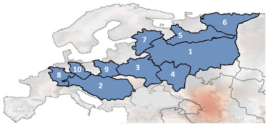
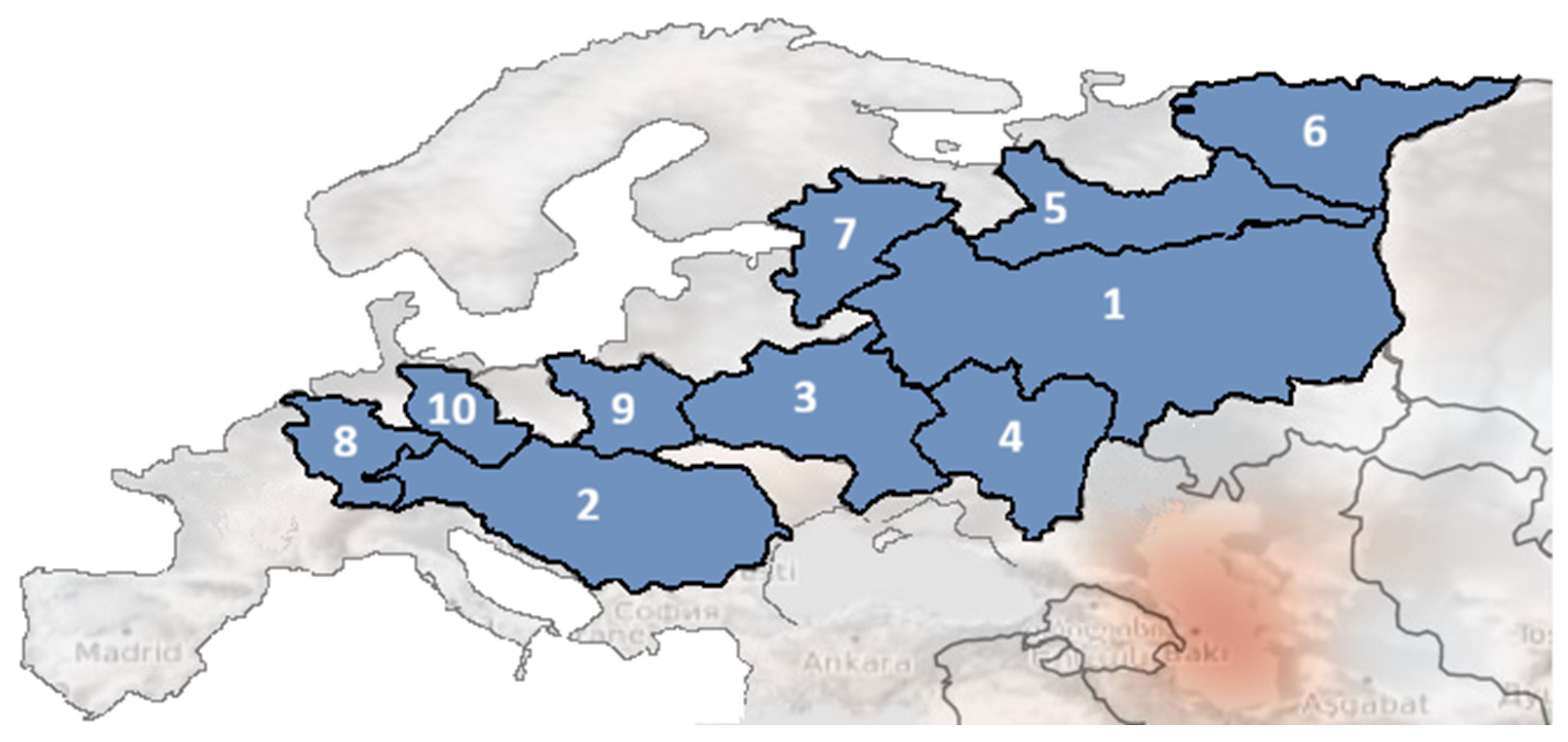
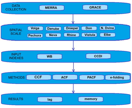
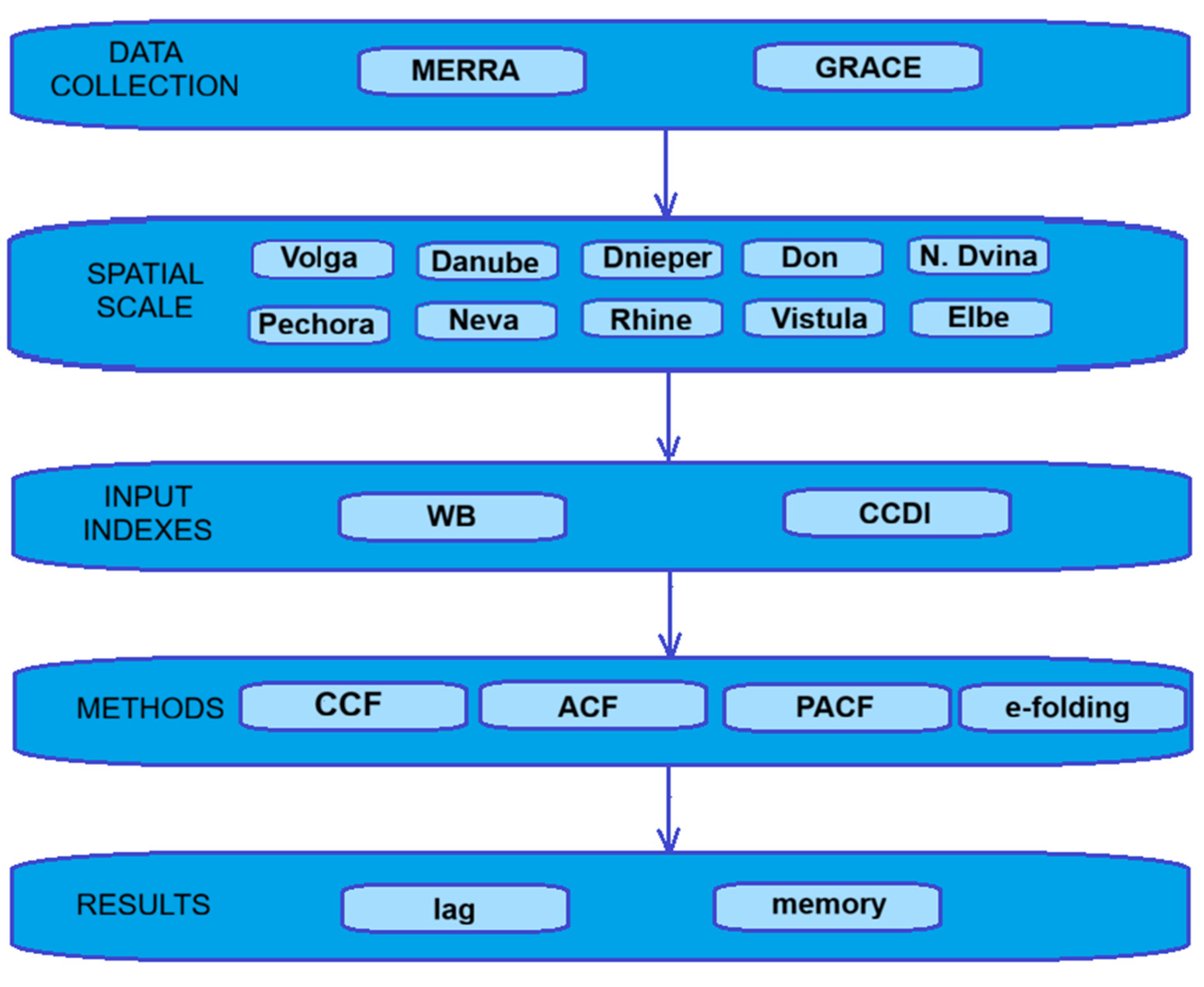
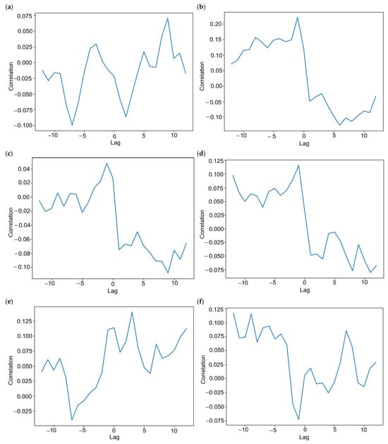
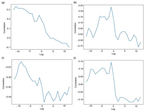
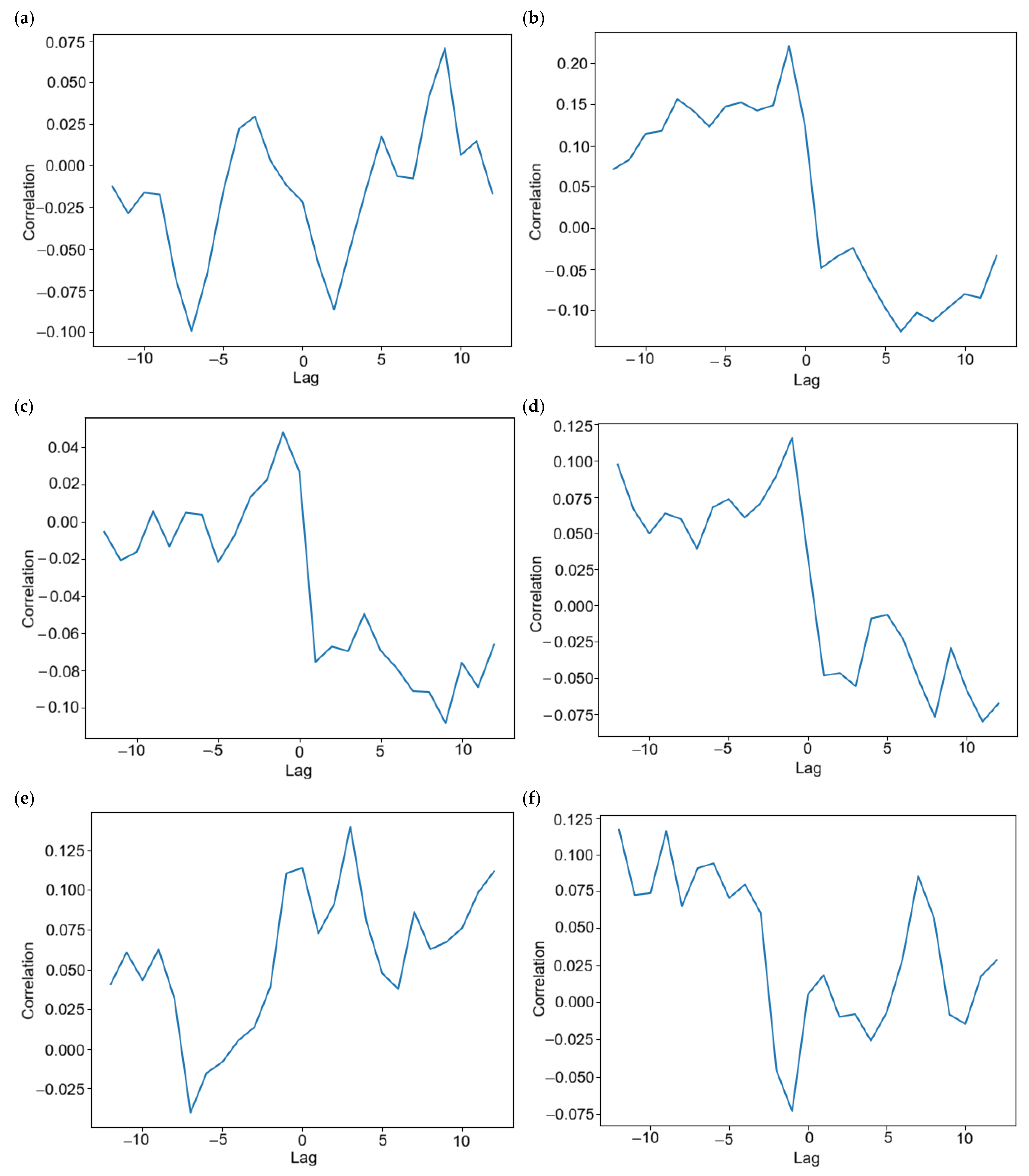
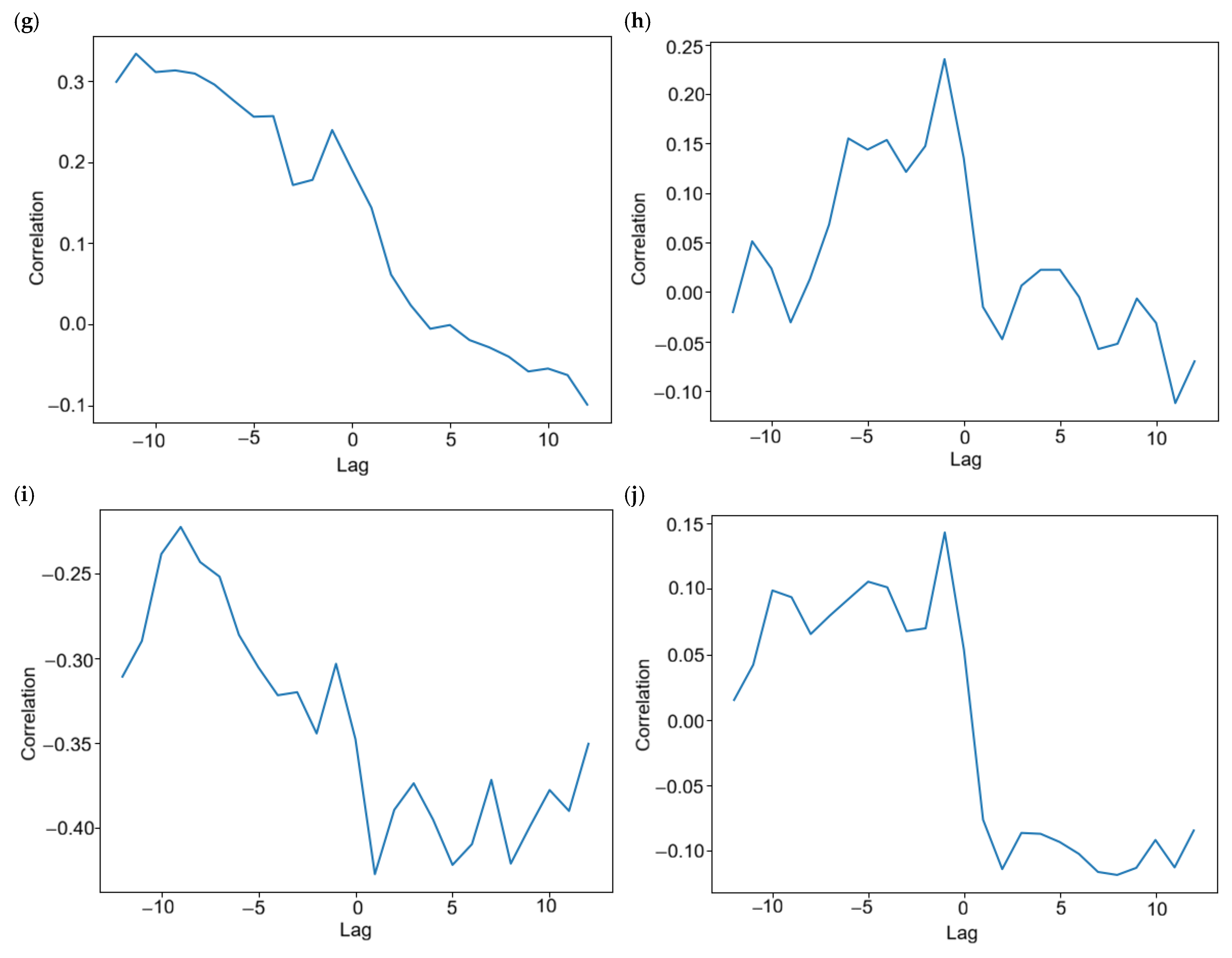
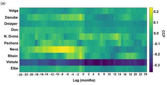
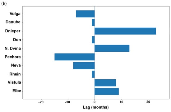
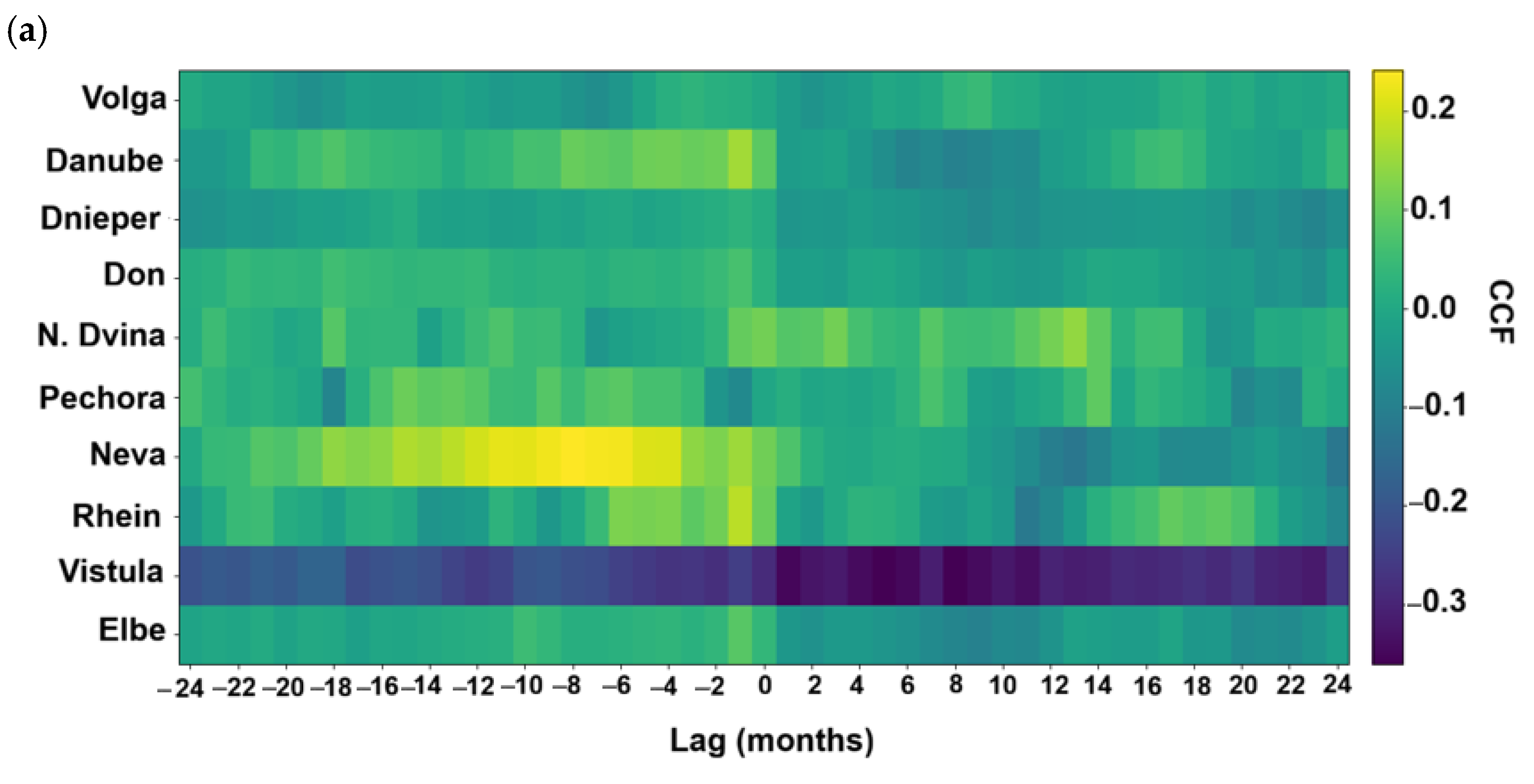
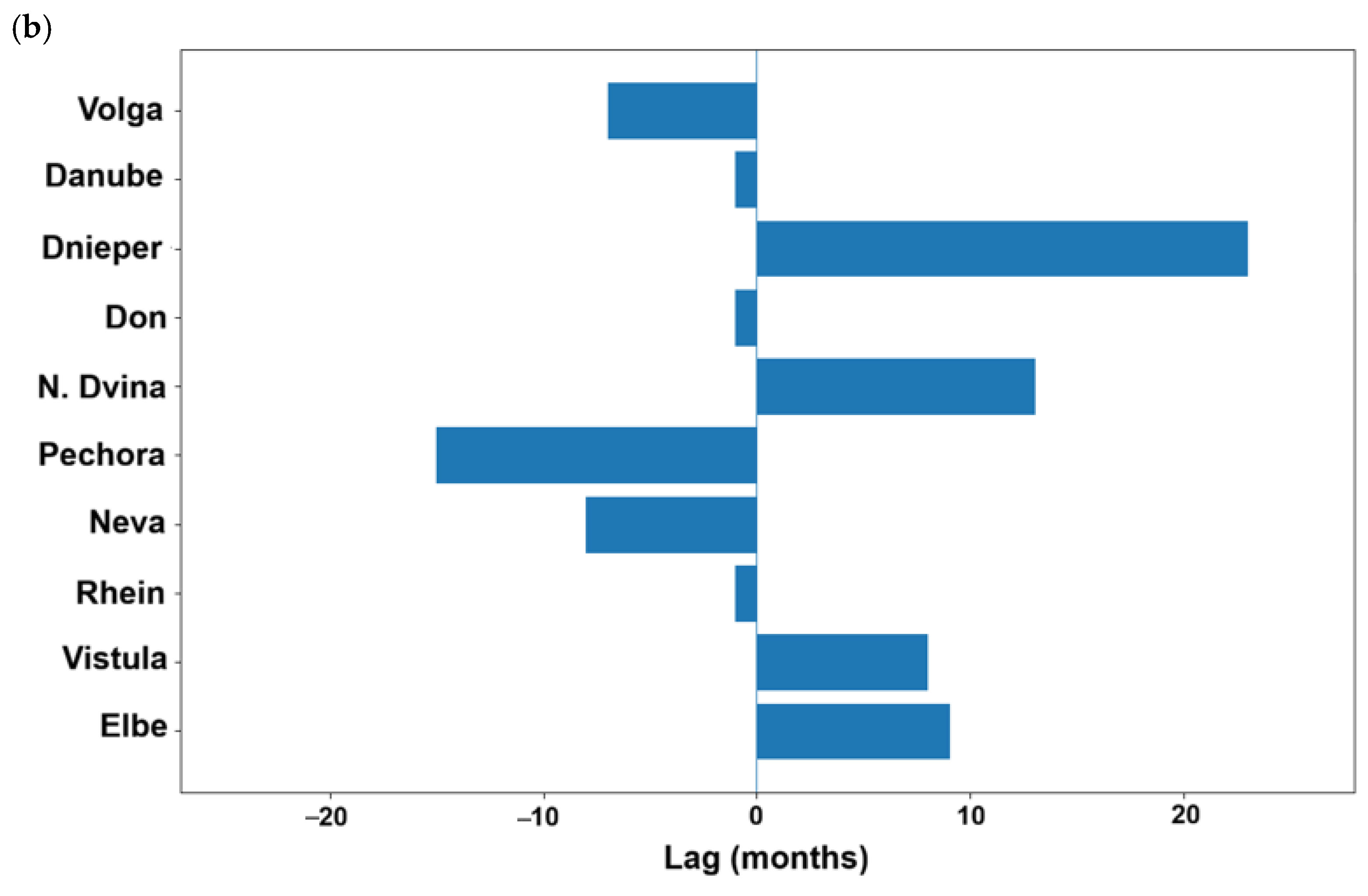
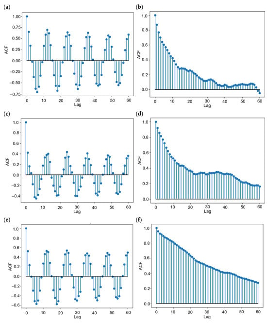
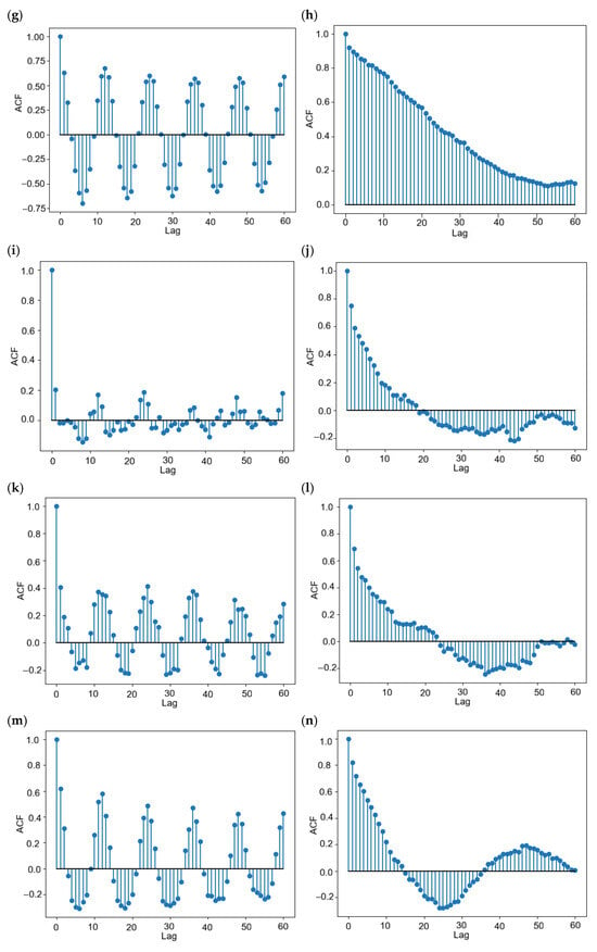
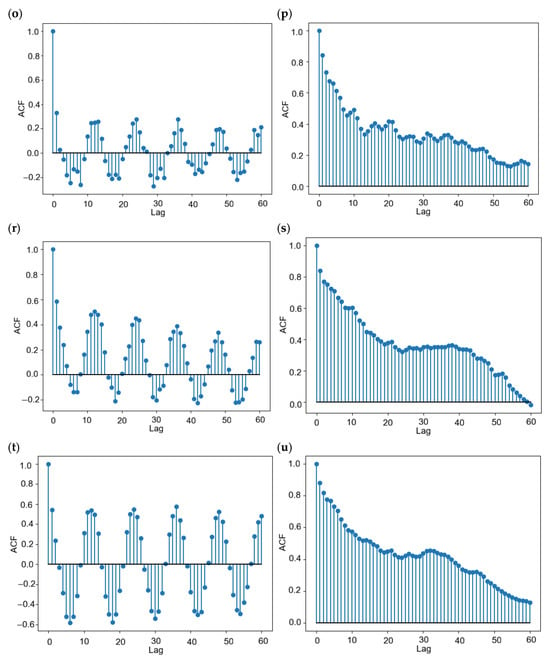
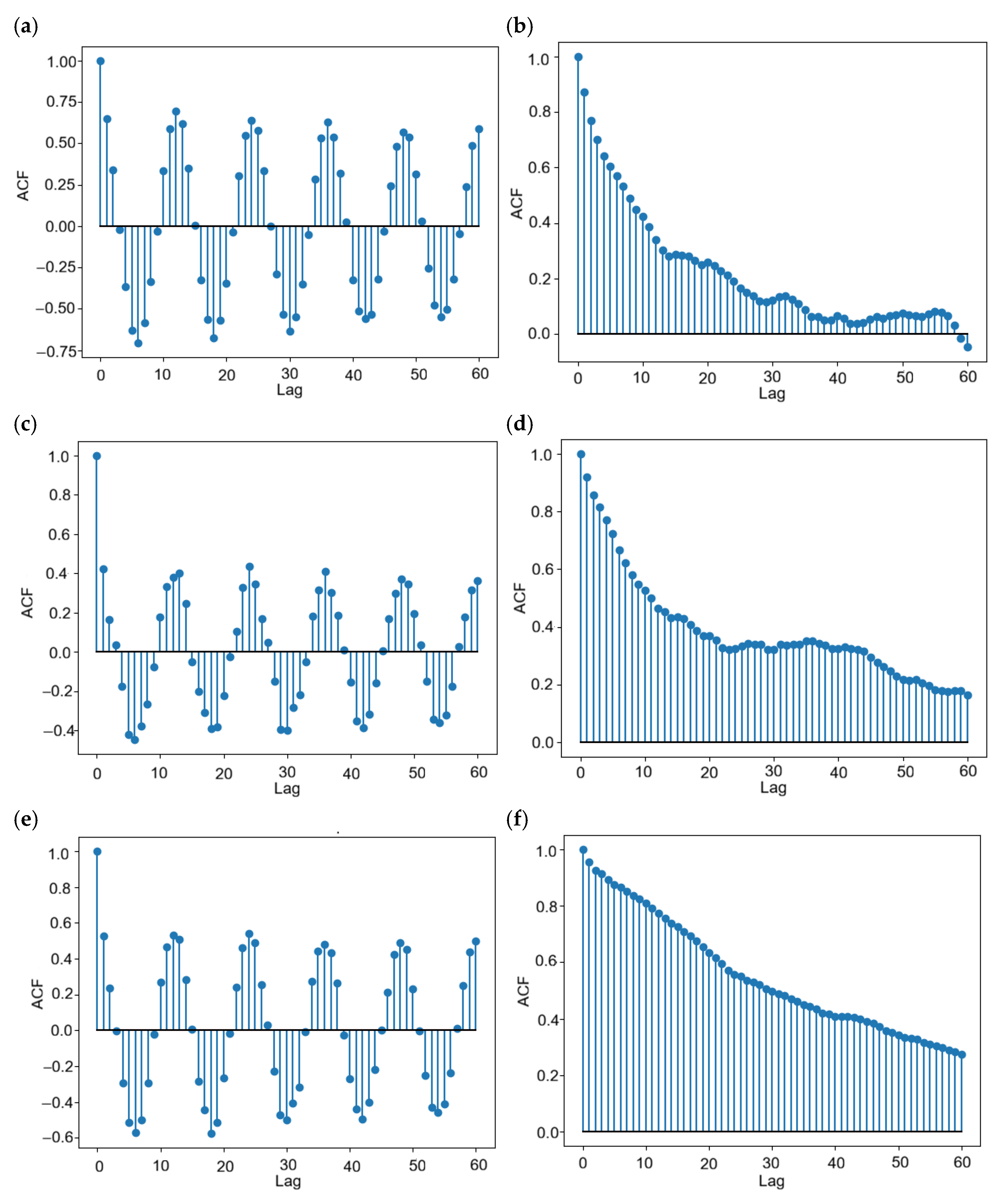
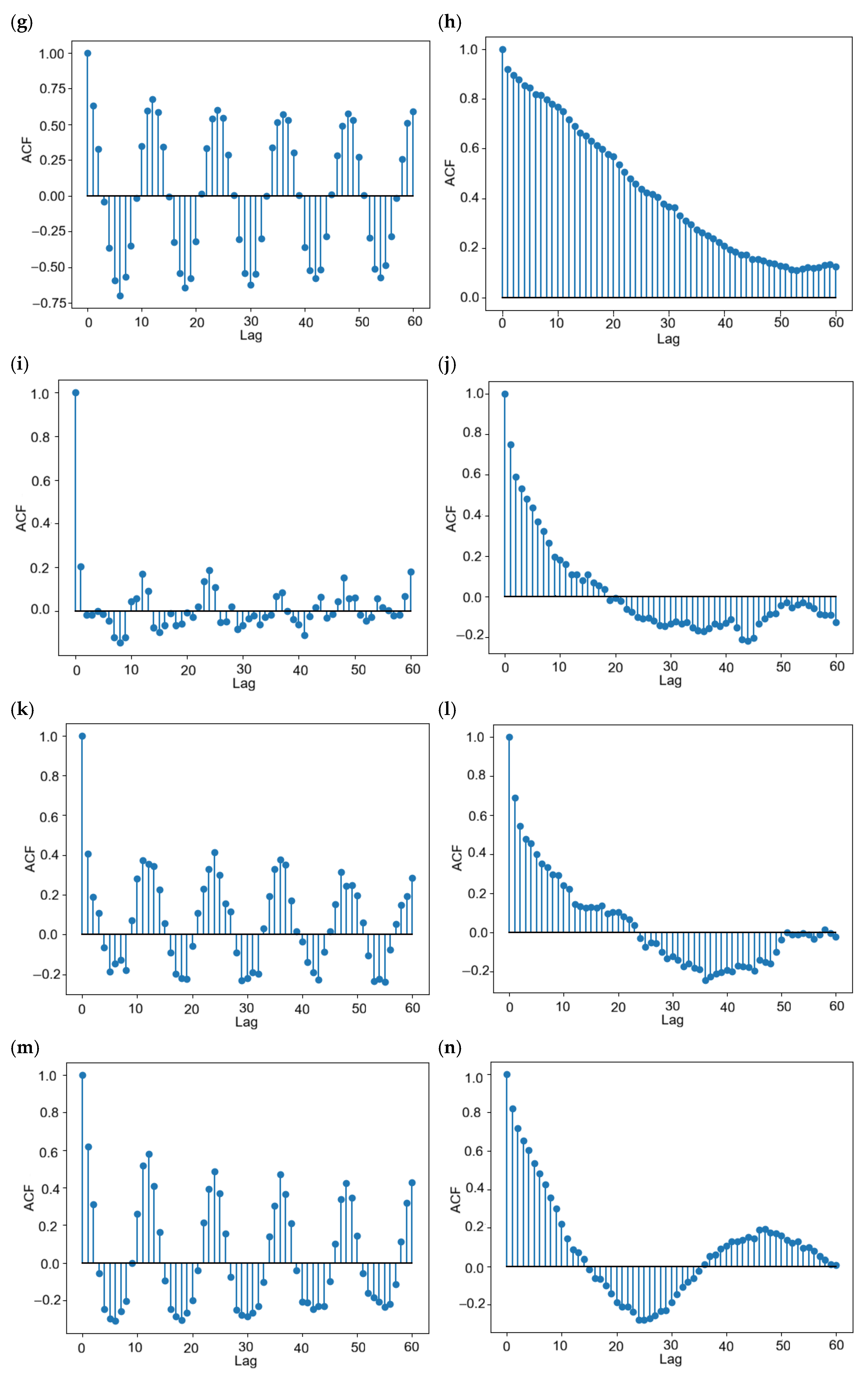
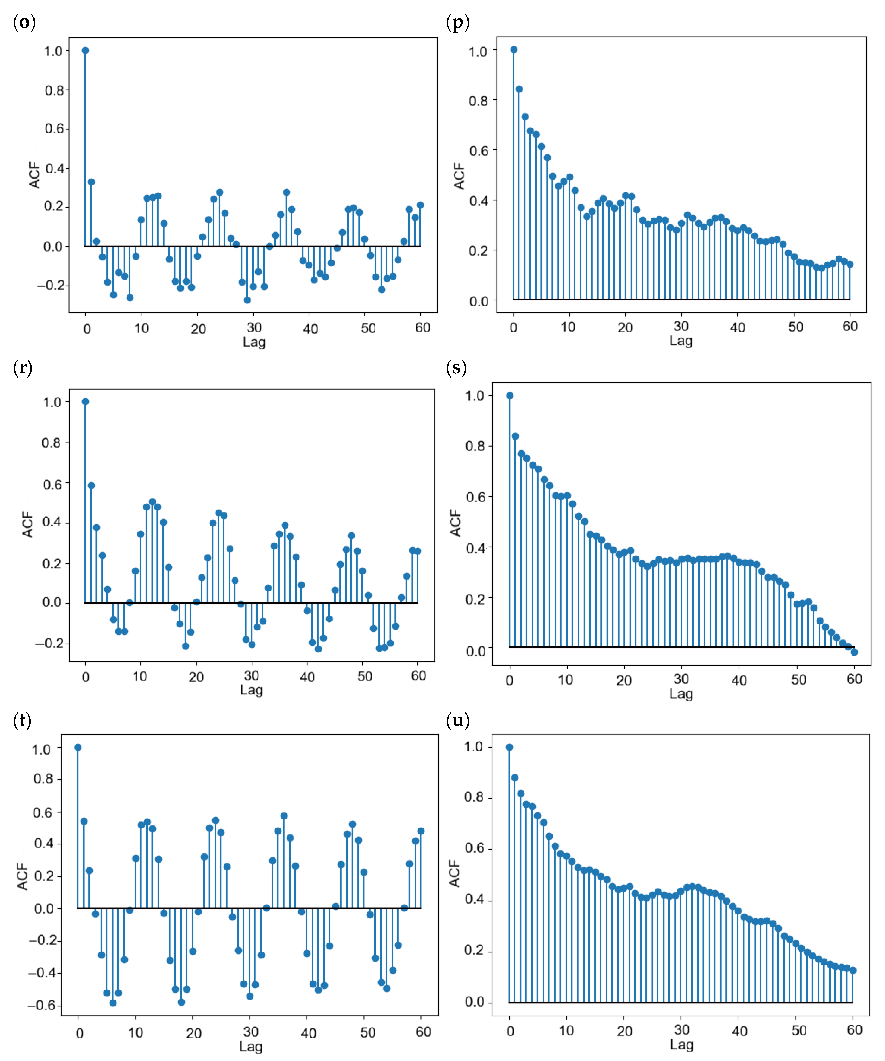
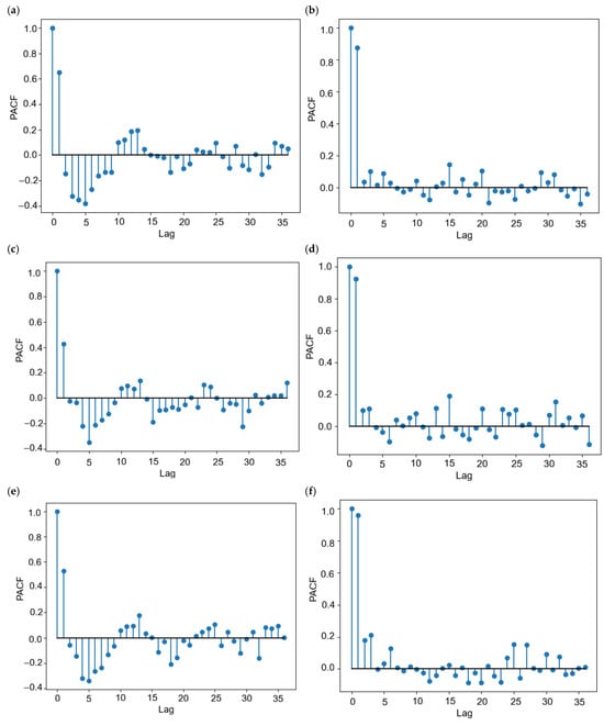
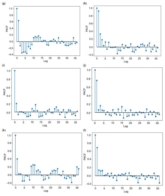
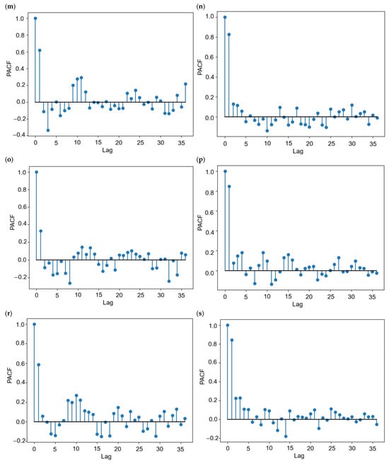
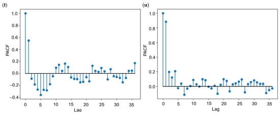
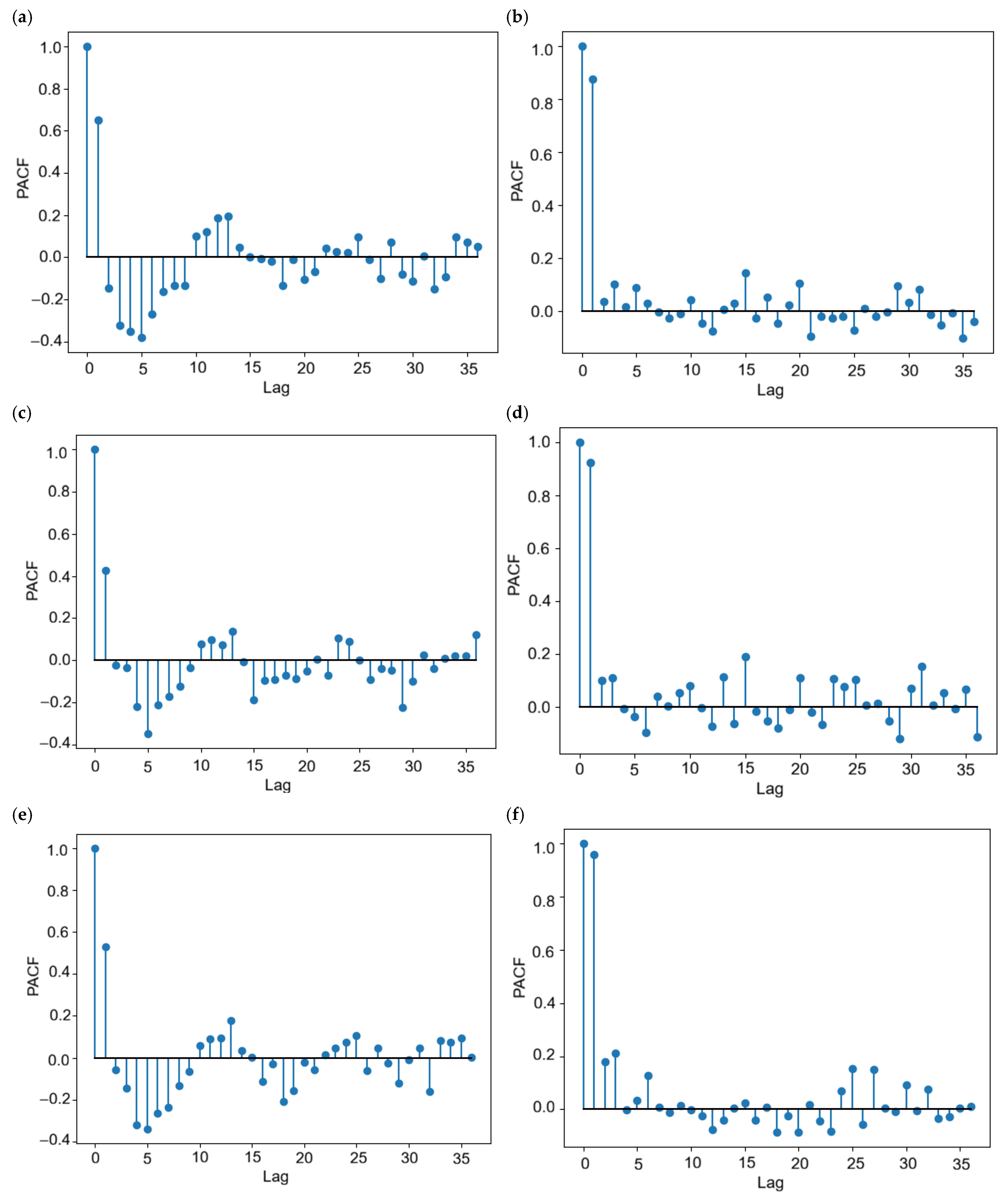
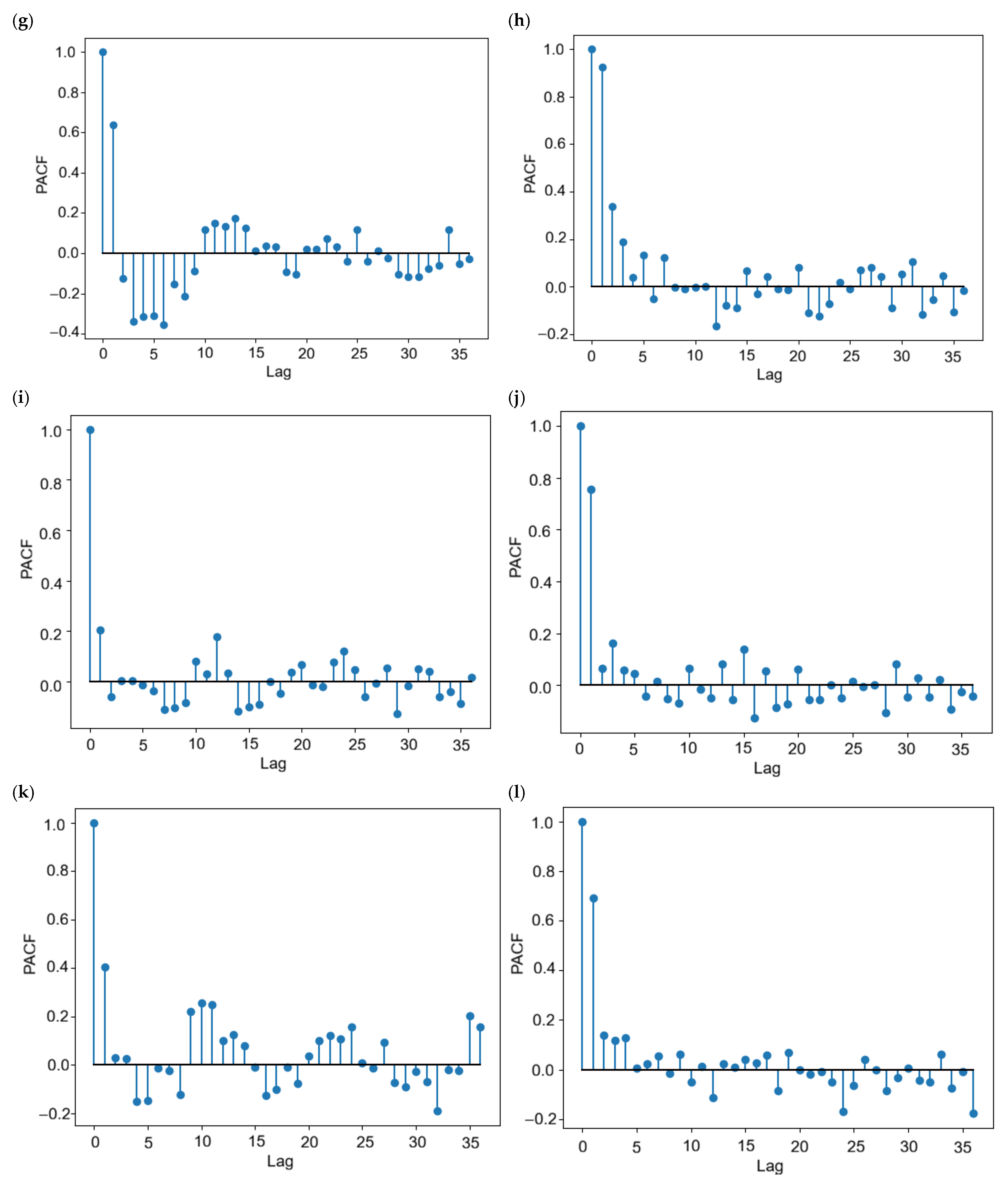
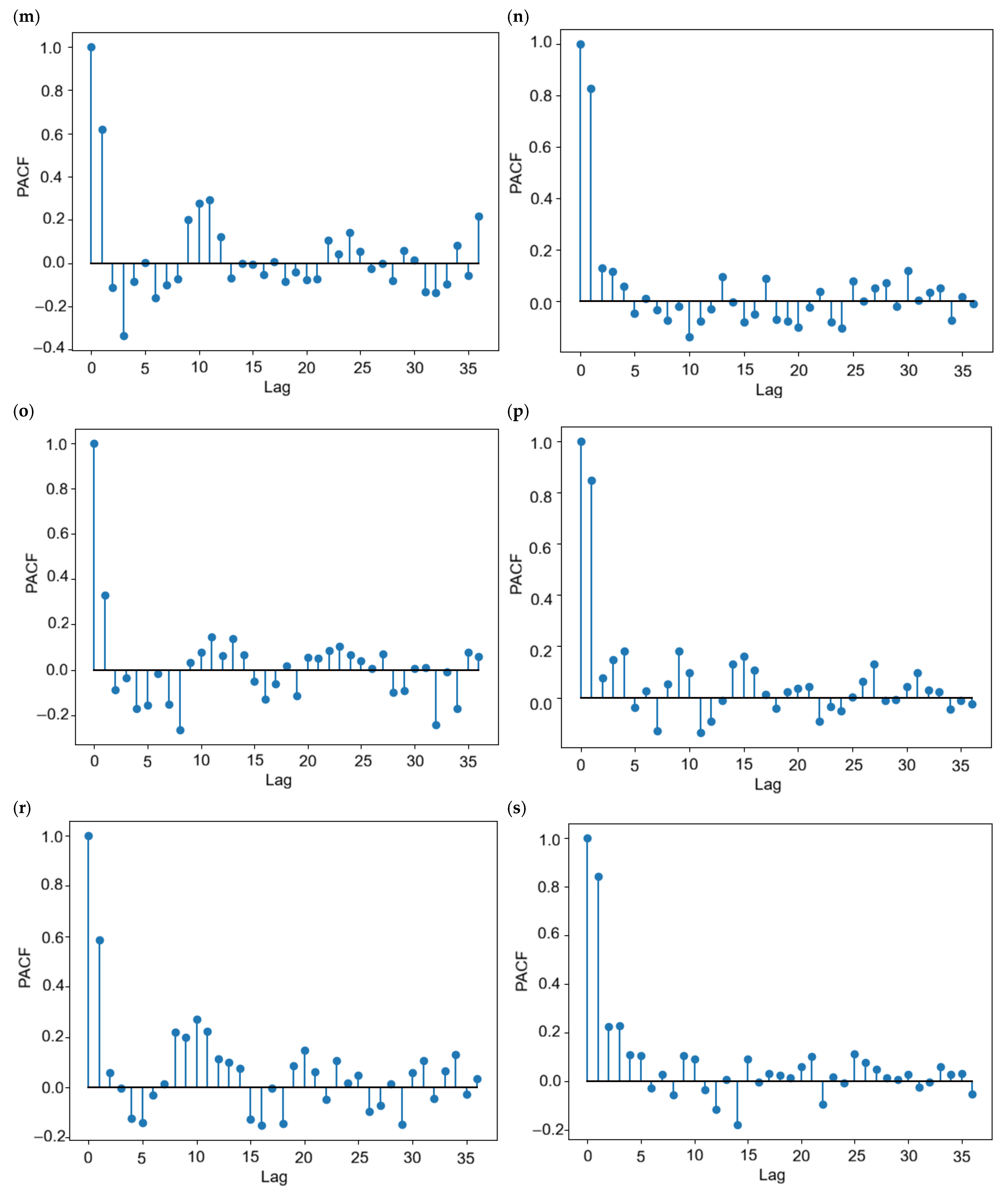
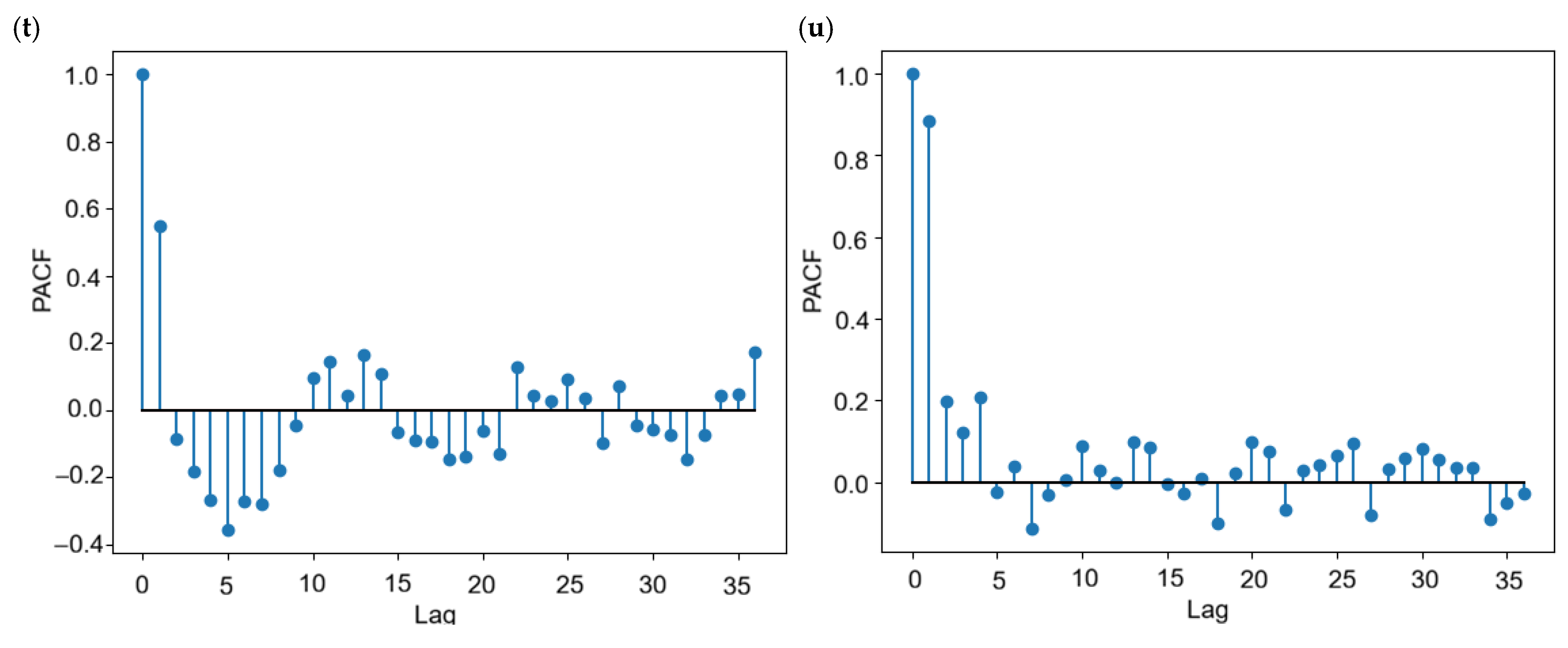
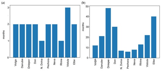
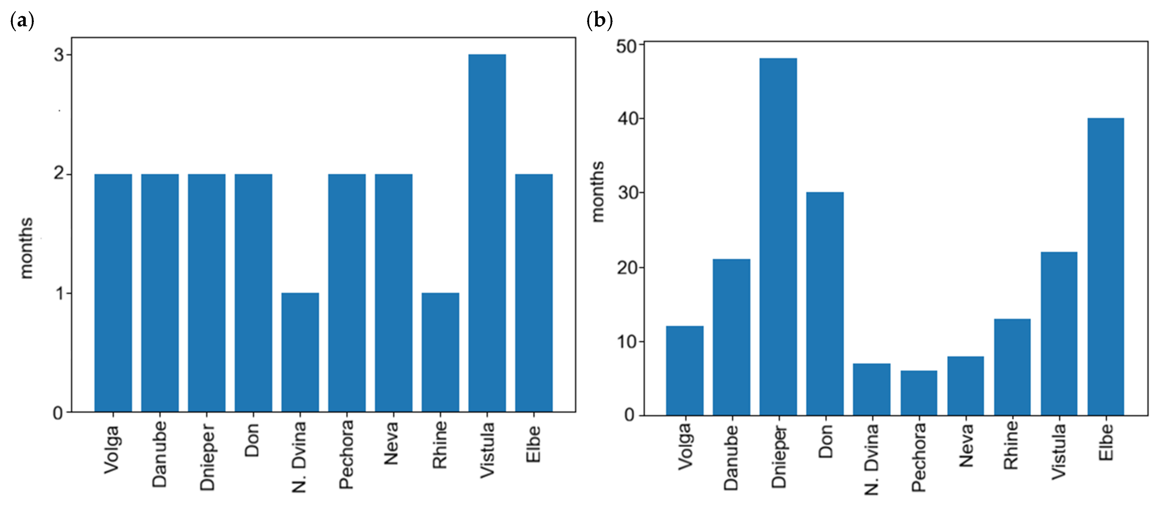
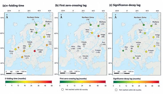
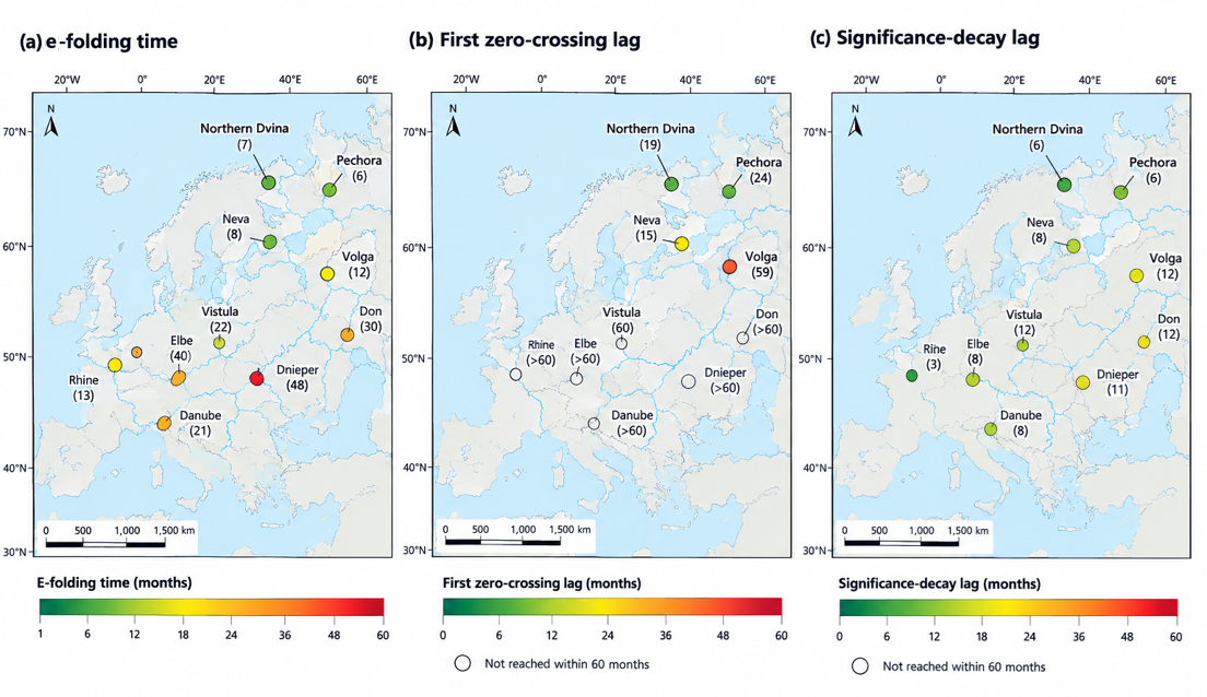

Disclaimer/Publisher’s Note: The statements, opinions and data contained in all publications are solely those of the individual author(s) and contributor(s) and not of MDPI and/or the editor(s). MDPI and/or the editor(s) disclaim responsibility for any injury to people or property resulting from any ideas, methods, instructions or products referred to in the content. |
© 2026 by the authors. Licensee MDPI, Basel, Switzerland. This article is an open access article distributed under the terms and conditions of the Creative Commons Attribution (CC BY) license.