


Abstract
Reliable multimodal image analysis is challenging when complementary sensors exhibit class-dependent strengths and local prediction uncertainty. This study presents a reliability-aware hybrid decision-fusion framework for fine-grained tidal-flat land-cover mapping as a demanding application of multisource image processing. A pyramid scene parsing network (PSPNet) with a 50-layer residual network (ResNet-50) backbone extracts multi-scale spatial context from high-resolution multispectral patches, while a Random Forest models 166-dimensional hyperspectral reflectance signatures. Instead of applying uniform score averaging, the framework combines validation-derived class reliability, pixel-level confidence, and branch disagreement to preserve trusted spatial predictions and selectively introduce spectral correction in uncertain regions; morphological refinement improves local mask continuity. Experiments used GF-2, GF-7, ZY1-02E/F, and ground-reference data acquired from 2022 to 2024, comprising 23 classes, 12,666 image samples, and 452,156 spectral samples. The method achieved 94.64% overall accuracy, 92.85% mean class recall (MCR), 85.47% mean intersection over union (mIoU), 91.72% macro-averaged F1 score (Macro-F1), and 85.88% Small-object F1. Relative to the PSPNet and Random Forest branches, mIoU increased by 4.73 and 3.84 percentage points, while Small-object F1 increased by 5.36 and 6.92 points. The results demonstrate that reliability-aware hybrid fusion can improve both spectrally ambiguous surface classification and spatially fragmented object recognition in complex multimodal scenes.
1. Introduction
Tidal flats are highly dynamic land–sea transition zones that support sediment exchange, coastal biodiversity, aquaculture production, shoreline protection, and coastal engineering. Their spatial extent and surface composition respond rapidly to tidal inundation, sediment transport, vegetation succession, reclamation, and intensive human disturbance. Satellite-based mapping has advanced through long-term Landsat archives, cloud-computing platforms, and increasingly detailed global and national products [1,2,3,4]. These datasets provide essential baselines for coastal monitoring, but they generally emphasize tidal-flat extent, wetland distribution, or broad land-cover groups. From an applied image-analysis perspective, a more difficult problem is to distinguish many natural and engineered categories that coexist at small spatial scales within fragmented coastal scenes.
Recent studies have improved coastal wetland interpretation using time-series imagery, deep learning, spectral endmember analysis, high-resolution observations, and hierarchical classification [5,6,7,8]. Nevertheless, fine-grained tidal-flat mapping requires more than increasing spatial detail. Practical coastal inventories may need to distinguish silt flat, rocky flat, bare land, aquaculture pond, aquaculture net, road, footpath, bridge, embankment, pier, dock, oil tank, and container yard in a single workflow. These categories differ in material composition, object scale, boundary continuity, morphology, and contextual relationships. The task is therefore a representative multimodal classification problem in which an applied computational framework must exploit both spectral separability and spatial structure.
One computational challenge is spectral ambiguity among natural and semi-natural surfaces. Wet silt flats, bare land, agricultural land, vegetation-related surfaces, and aquaculture ponds can exhibit similar appearances in multispectral images because of moisture variation, sediment background, vegetation coverage, and tidal exposure. Hyperspectral observations provide densely sampled reflectance information and can improve discrimination of classes with subtle material or moisture differences; accordingly, joint multispectral–hyperspectral classification, multi-resolution collaborative fusion, and ZY1-02D hyperspectral wetland mapping have received growing attention [9,10,11,12]. Attention and self-attention architectures have further improved spectral–spatial representation for wetland classification [13,14]. However, hyperspectral classification remains affected by mixed pixels, coarser spatial representation, and limited preservation of narrow-object geometry.
A second challenge is spatial fragmentation and small-object recognition. High-resolution multispectral imagery is well suited to boundary extraction, local texture analysis, and contextual reasoning for roads, footpaths, bridges, embankments, piers, docks, and aquaculture facilities. Recent wetland and hyperspectral studies have introduced cross-domain feature fusion, adversarial domain adaptation, dynamic graph learning, feature disentanglement, Swin Transformer architectures, and Segment Anything Model-assisted CNN–Transformer systems [15,16,17,18,19,20]. These approaches demonstrate the value of advanced artificial intelligence for complex geospatial images. Yet many methods concentrate on feature representation or domain transfer, while the final decision stage still relies on fixed feature fusion, direct score integration, or a single end-to-end output. In heterogeneous tidal-flat scenes, the practical question is also when a spatial decision should be retained and when spectral evidence should be used to correct it.
More broadly, multispectral–hyperspectral fusion is a multimodal information-processing problem in which one source generally provides finer spatial structure and the other richer spectral content [21,22,23,24]. Existing solutions include feature concatenation, multi-stream neural networks, low-rank reconstruction, interpretable deep fusion, and transformer-based spatial–spectral interaction. Recent attention- and self-attention-based spectral–spatial models [13,14], transformer-based multispectral–hyperspectral fusion [24], and uncertainty-aware dynamic multimodal fusion [25] have further shifted the field from static information combination toward adaptive cross-modal interaction and reliability-sensitive weighting. Earlier decision-fusion studies also provide important methodological precedents. Fauvel et al. [26] incorporated class- and classifier-dependent prior reliability together with pixelwise fuzzy uncertainty into adaptive decision fusion, while Hu et al. [27] employed fuzzy-membership-based decision fusion of object-specific CNN classifiers for coastal wetland hyperspectral classification. Accordingly, class-dependent reliability, pixel-level confidence, and agreement-aware decision handling are regarded as established concepts rather than individual methodological innovations. The specific contribution of the present framework lies in their integration into a calibrated, two-stage decision procedure for multispectral and hyperspectral observations with different spatial resolutions. Spatial predictions are retained unchanged only when interbranch agreement and the calibrated spatial-confidence threshold are simultaneously satisfied; otherwise, complementary spectral evidence is incorporated through class-wise reliability- and confidence-weighted probability fusion. This procedure explicitly separates the decision of whether to modify a spatial prediction from the subsequent weighting of complementary evidence. Engineered coastal objects with recognizable shapes may be more reliably identified by spatial segmentation, whereas sedimentary and vegetation-related surfaces may benefit more from hyperspectral signatures. For heterogeneous tidal-flat scenes, the resulting design aims to preserve reliable spatial structures while selectively correcting predictions affected by spectral ambiguity or classification uncertainty.
Semantic segmentation and ensemble learning provide complementary building blocks for such a system. Remote sensing image analysis increasingly emphasizes multi-scale structures, tiny targets, and fine-grained recognition in cluttered scenes [28]. PSPNet aggregates local and global context through pyramid pooling [29], and residual learning supports stable deep feature propagation [30]. Random Forest remains an effective ensemble classifier for high-dimensional spectral vectors because it represents nonlinear decision boundaries with comparatively robust generalization [31]. Class-balanced learning is important when dominant areal classes can suppress minority categories [32], while fine-grained object-detection research shows that small objects in complex backgrounds require careful feature balancing and label assignment [33]. These techniques are individually well established, but their integration does not by itself resolve how branch-specific evidence should be selected at the decision level.
Accordingly, the research gap addressed in this study is more specific: how to convert class-dependent branch competence and pixel-dependent prediction certainty into an explicit decision rule for fine-grained spatial–spectral mapping. In heterogeneous tidal-flat scenes, spectrally ambiguous natural surfaces coexist with narrow engineered structures, so indiscriminate multimodal correction may disturb reliable object geometry, whereas insufficient correction may leave material-related spectral confusion unresolved. The fusion mechanism therefore needs not only to determine how much each branch should contribute, but also to determine when complementary spectral evidence should intervene and when a trusted spatial decision should remain unchanged.
To address this gap, this study develops a reliability-aware, confidence-guided hybrid decision-fusion framework for fine-grained tidal-flat land-cover mapping using multispectral imagery, hyperspectral signatures, and ground validation. The contribution is positioned as a decision-fusion methodology and its application to fine-grained tidal-flat mapping, rather than as a claim that PSPNet, Random Forest, confidence estimation, disagreement detection, or morphological operations are individually novel. The methodological contribution lies in coupling these established components into a reliability-gated decision process that explicitly distinguishes predictions that should be preserved from those that require complementary spectral correction. A PSPNet branch extracts multi-scale spatial context from high-resolution images, and a Random Forest branch models class probabilities from 166-dimensional hyperspectral reflectance vectors. The fusion module combines validation-derived class reliability, pixel-level confidence, and branch disagreement to partition the map into trusted spatial zones and validation-required zones. Spatial predictions are preserved where structural evidence is reliable, whereas spectral correction is selectively activated in uncertain regions. Morphological refinement is subsequently used as a conventional post-fusion regularization step to improve local continuity and is evaluated separately rather than treated as the principal source of methodological novelty.
The main contributions of this study to applied multimodal image processing are summarized as follows.
- (1)
- A task-decomposed multimodal mapping framework is established in which high-resolution multispectral imagery and hyperspectral reflectance are processed by dedicated spatial and spectral branches. This separation makes their class-dependent competence observable before fusion and provides the basis for reliability-aware decision making.
- (2)
- The core methodological contribution is a reliability-gated decision rule that jointly uses class-wise validation performance, pixel-level confidence, and branch disagreement to distinguish trusted spatial zones from validation-required zones. Unlike uniform late fusion or globally applied adaptive weighting, the rule preserves high-confidence spatial decisions and selectively activates hyperspectral correction only where additional evidence is required.
- (3)
- The framework is evaluated on GF-2, GF-7, ZY1-02E/F, and ground-reference data acquired from 2022 to 2024 for 23 land-cover classes. Overall, class-wise, ablation, small-object, visual, and confusion-matrix analyses are used to assess both algorithmic effectiveness and practical mapping performance. The evaluation deliberately includes both spectrally ambiguous natural surfaces and narrow engineered coastal objects, allowing the proposed decision policy to be examined under two contrasting sources of classification difficulty.
The remainder of this paper is organized as follows. Section 2 describes the study area, multisource data, preprocessing, sample construction, branch models, reliability-aware fusion strategy, and evaluation metrics. Section 3 presents and discusses preprocessing quality, training behavior, branch complementarity, overall and class-wise performance, ablation results, visual mapping, and limitations. Section 4 summarizes the conclusions and future directions.
2. Materials and Methods
2.1. Study Area and Data Sources
The study area is located in Sanggou Bay, Rongcheng City, at the eastern end of the Shandong Peninsula, China, and faces the Yellow Sea. The investigated coastal zone extends approximately from 37°01′ to 37°09′ N and from 122°24′ to 122°35′ E. Sanggou Bay is a shallow, semi-enclosed coastal embayment with an area of approximately 144 km2 and an average water depth of about 7.5 m. Hydrodynamic exchange is dominated by an irregular semidiurnal tidal regime, with a mean tidal range of approximately 2.0 m. The shoreline and adjacent intertidal zone contain silt flats, rocky shores, vegetation, agricultural land, intensive aquaculture, transportation corridors, coastal engineering structures, industrial facilities, and port-related objects. This juxtaposition of spectrally similar natural surfaces and geometrically fragmented engineered objects provides a particularly demanding setting for evaluating spatial–spectral fusion. The area was therefore selected not merely as a representative tidal-flat site, but because it simultaneously contains the two principal sources of classification difficulty addressed in this study: material-related spectral ambiguity and small-object spatial fragmentation. The geographic location, study extent, and representative land-cover configuration are shown in Figure 1.
Figure 1.
Location and land-cover context of the study area in Sanggou Bay, eastern Shandong Peninsula, China: (a) regional location of Sanggou Bay; (b) geographic extent of the study area; (c) representative GF-2 imagery showing the classification area, tidal flats, aquaculture areas, and typical artificial coastal structures.
Multispectral and hyperspectral satellite images acquired from 2022 to 2024 were used in this study. The multispectral data included GF-2 and GF-7 imagery, and the hyperspectral data were obtained from ZY1-02E/F satellites. GF-2 provides 4 m multispectral imagery and 0.8 m panchromatic imagery, which were mainly used for spatial feature extraction and fine-structure delineation. GF-7 imagery was used to support geometric consistency checking and auxiliary interpretation. ZY1-02E/F hyperspectral imagery provides 166 spectral bands covering 400–2500 nm, which were used for spectral discrimination of visually similar land cover classes. Ground reference data were used for sample labeling, validation, and accuracy assessment. Because exact temporal coincidence among the three satellite systems was not always available, the observations were organized into temporally matched acquisition groups rather than treated as strictly simultaneous measurements. Primary scenes were selected from late-summer to early-autumn acquisition windows in 2022–2024, when vegetation development and aquaculture activity were relatively comparable among years. For multimodal pairing, the nearest available multispectral and hyperspectral observations were preferentially selected within the same seasonal window, and scenes affected by substantial cloud cover, strong tidal inundation, recent rainfall, or visually evident short-term surface disturbance were excluded. The retained coastal scenes primarily represented low-to-middle tidal conditions, thereby reducing differences in exposed tidal-flat area and sediment moisture caused solely by tidal stage. The main datasets are summarized in Table 1.
Table 1.
Summary of remote sensing and reference datasets used in this study.
As shown in Table 1, the multispectral and hyperspectral datasets provide complementary information. GF-2 and GF-7 imagery mainly support the PSPNet spatial branch, whereas ZY1-02E/F hyperspectral imagery supports the Random Forest spectral branch.
2.2. Land Cover Classification System
A 23-class tidal-flat land-cover classification system was established with reference to the Chinese national standard GB/T 21010-2017 [34], Current Land Use Classification, and was further adapted to the fine spatial resolution and engineering complexity of the study area. The resulting system is therefore a project-specific fine-grained interpretation scheme rather than a direct reproduction of the national standard. Compared with coarse coastal wetland mapping, this classification system is designed to evaluate fine-grained recognition under complex spatial and spectral conditions. Project-specific attribute codes, such as 71–73 for transportation-related objects, 131–132 for dock/boat objects, 141–143 for pier types, and 151–152 for aquaculture facilities, were introduced only as internal subclass identifiers and do not represent national-standard codes. Fine-grained subclasses were retained only when they could be consistently distinguished from GF-2/GF-7 imagery using object shape, relative width, connectivity, shoreline position, surrounding land use, and ground-supported interpretation. The complete land cover categories, attribute codes, annotation criteria, and sample quantities are listed in Table 2.
Table 2.
Land cover categories, attribute codes, and sample quantities used in this study.
For annotation, class assignment was based on a hierarchical combination of morphology, spatial context, spectral characteristics, and temporal stability rather than on a single visual cue. For easily confused linear objects, relative width, continuity, orientation, connectivity, and functional context were considered jointly. Pier subclasses were distinguished primarily by their orientation and geometric relationship with the shoreline, while aquaculture and port-related classes were identified using both repetitive structural patterns and surrounding functional context. Ambiguous boundary pixels and objects whose class identity could not be consistently confirmed across the available high-resolution and reference observations were excluded from the labeled dataset. For hyperspectral sample extraction, each 30 m AHSI pixel footprint was intersected with the high-resolution reference polygons on the common geographic grid. A conservative purity criterion was applied: a spectral sample was retained only when a single target class occupied at least 70% of the hyperspectral pixel footprint, whereas pixels crossing class boundaries or containing no dominant class were excluded. Each retained hyperspectral pixel was then linked to the 512 × 512 GF-2 image patch containing its footprint center, thereby establishing an explicit spatial correspondence between the spectral sample and the spatial prediction. For intrinsically narrow engineered objects that were frequently affected by mixed-pixel effects, the spectral branch was treated as complementary rather than primary evidence, and its influence was further regulated by the class-wise reliability coefficient during decision fusion.
As shown in Table 2, the dataset contains 12,666 image samples and 452,156 spectral samples. The image samples were used for the PSPNet spatial branch, and the spectral samples were used for the Random Forest spectral branch. The class system includes both large-area tidal flat surfaces and small engineered objects, which allows the proposed fusion framework to be evaluated under class imbalance, spectral similarity, and spatial fragmentation.
2.3. Image Preprocessing and Co-Registration
All remote sensing images were preprocessed before sample extraction and model training. The preprocessing workflow included radiometric calibration, atmospheric correction, geometric correction, panchromatic–multispectral fusion, coordinate projection, and multisource co-registration. Radiometric and atmospheric corrections were applied to improve surface reflectance consistency. For GF-series multispectral images, atmospheric correction was performed using the FLAASH model. For ZY1-02E/F hyperspectral images, radiometric correction, abnormal-band checking, and spectral normalization were conducted before spectral feature extraction. The ZY1-02E/F hyperspectral data have a native spatial resolution of approximately 30 m. Therefore, the pan-sharpened GF-2 imagery was treated as the high-resolution spatial reference, whereas the hyperspectral reflectance vectors were retained at their native spatial support. GF-7 imagery was used for geometric consistency checking and auxiliary interpretation and was not directly used as an input feature of either classification branch.
GF-2 panchromatic and multispectral images were fused using the NNDiffuse method to enhance spatial details while preserving spectral fidelity. Geometric correction and orthorectification were performed using satellite orbital information, ground control information, and digital elevation data. All datasets were projected to the WGS 84/UTM Zone 51N coordinate system and subsequently co-registered under a common geographic reference framework. After initial orthorectification, image-to-image registration was refined using 30 well-distributed tie points selected from temporally stable coastal features, including road intersections, bridge endpoints, embankment corners, aquaculture-pond boundaries, and industrial facilities. An additional 12 independent checkpoints, which were not involved in the transformation, were used to evaluate registration accuracy. The final root-mean-square co-registration error between the GF-2 reference imagery and the ZY1-02E/F hyperspectral data was 11.4 m, corresponding to approximately 0.38 hyperspectral pixels and remaining below one-half of the native AHSI pixel size. Stable coastal structures, including roads, bridges, embankments, aquaculture pond boundaries, and industrial facilities, were used as reference objects to check spatial alignment.
Differences in spatial resolution were handled without artificially increasing the spatial information content of the hyperspectral imagery. The Random Forest branch operated directly on the native 30 m hyperspectral reflectance vectors; the raw spectra were not interpolated to the GF-2 pixel size. During decision fusion, only the Random Forest class-probability vector was spatially transferred to the high-resolution reference grid according to the registered footprint of each hyperspectral pixel. High-resolution GF-2 pixels falling within the same hyperspectral footprint therefore shared the corresponding spectral probability vector, while their spatial labels and boundaries continued to be determined independently by the PSPNet branch. This footprint-based correspondence avoids introducing artificial subpixel spectral detail while allowing the two branches to be combined within a common geographic framework. The final 23-class land-cover map was generated on the pan-sharpened GF-2 reference grid with a nominal pixel spacing of 0.8 m. This output resolution represents the spatial sampling grid of the classification map, whereas the hyperspectral information retained its native 30 m spatial support without introducing artificial subpixel spectral detail.
Images affected by severe cloud cover, obvious tidal inundation, unclear land–water boundaries, or large geometric mismatch were excluded from the final dataset. This preprocessing procedure ensured that the spatial predictions from high-resolution multispectral imagery and the spectral predictions from hyperspectral imagery could be integrated consistently in the subsequent fusion stage.
2.4. Sample Annotation and Dataset Construction
Based on the 23-class classification system listed in Table 2, image samples and spectral samples were constructed through visual interpretation, spectral inspection, and ground-supported reference checking. GF-2 and GF-7 images were used to delineate object boundaries and spatial structures, while ZY1-02E/F hyperspectral data were used to check the spectral consistency of visually similar classes.
A total of 12,666 image samples and 452,156 spectral samples were organized for model development. Image samples were used to train and evaluate the PSPNet spatial branch, whereas spectral samples were used to train and evaluate the Random Forest spectral branch. To prevent spatial information leakage, the training, testing, and validation subsets were constructed using a geographically disjoint block- and polygon-level partition rather than random pixel- or patch-level splitting. The annotated area was first divided into non-overlapping geographic blocks, and each labeled polygon was assigned in its entirety to only one subset. All image patches and hyperspectral samples derived from the same polygon therefore inherited the same subset assignment. The same geographic-block and reference-polygon assignments were applied to both the PSPNet and Random Forest branches before GF-2 image-patch cropping and ZY1-02E/F spectral-sample extraction, ensuring that spatially corresponding observations inherited identical partition labels. The blocks were allocated to the training, testing, and validation subsets at approximately 70%, 20%, and 10%, respectively, while class stratification was applied at the block/polygon assignment stage to maintain representation of all 23 classes. Overlapping image patches were restricted to individual data partitions, and GF-2 patches or 30 m hyperspectral pixel footprints spanning different partitions were excluded from sample extraction to prevent cross-partition spatial leakage. The test blocks were held out from model fitting, class-reliability estimation, and threshold selection, thereby providing a spatially independent evaluation of model performance [35,36]. Temporal consistency was checked before constructing paired spatial–spectral samples. Because multispectral, hyperspectral, and reference observations were not necessarily acquired on the same day, labels were transferred across sensors only when the land-cover identity and boundary geometry remained stable within the matched acquisition window. Particular attention was given to tidal-flat exposure, sediment moisture, seasonal vegetation, aquaculture ponds and nets, and actively modified coastal facilities. Pixels or objects showing detectable inundation changes, vegetation-state transitions, aquaculture reconfiguration, construction activity, or other land-cover changes between the paired observations were excluded from cross-modal sample construction rather than being forced to share a common label. This procedure reduced label noise caused by temporal mismatch while retaining the complementary spatial and spectral information required by the two branches.
During annotation, ambiguous boundary pixels, cloud-affected regions, shadow-contaminated areas, mixed tidal surfaces, and unstable tidal water coverage were excluded where possible. For narrow artificial classes, such as roads, footpaths, bridges, embankments, and piers, object continuity and local context were considered during labeling. For spectrally similar classes, such as silt flat, bare land, agricultural land, and forest and grassland, hyperspectral reflectance curves were used as auxiliary evidence. This annotation strategy provided separate but complementary inputs for the spatial and spectral branches of the proposed framework.
2.5. Overall Framework of the Proposed Method
To integrate the complementary advantages of multispectral and hyperspectral imagery, a confidence-guided spatial–spectral fusion framework was developed for fine-grained tidal flat land cover mapping. The overall workflow is shown in Figure 2.
Figure 2.
Overall framework of the proposed confidence-guided spatial–spectral fusion method. Solid arrows indicate the main data-processing workflow, while dashed lines indicate auxiliary relationships involving reference-label checking and cross-modal sample association.
As shown in Figure 2, the proposed framework consists of three main stages: data preparation, dual-branch prediction, and adaptive spatial–spectral fusion. In the data preparation stage, GF-2/GF-7 multispectral images, ZY1-02E/F hyperspectral images, and ground reference data were preprocessed and organized into image samples, spectral samples, and training/testing/validation subsets. The multispectral data mainly provided spatial structures and object boundaries, whereas the hyperspectral data provided high-dimensional spectral features for material discrimination.
In the dual-branch prediction stage, two complementary classifiers were constructed. The PSPNet spatial branch used high-resolution multispectral image patches to extract multi-scale contextual features and generate spatial classification probabilities. The Random Forest spectral branch used 166-dimensional hyperspectral reflectance vectors to learn nonlinear spectral decision boundaries and generate spectral class probabilities. The spatial branch was designed to improve boundary and structural representation, while the spectral branch was designed to enhance the separability of visually similar land cover classes.
In the adaptive fusion stage, the outputs of the two branches were integrated through a confidence-guided decision strategy. Class-wise reliability, pixel-level confidence, and branch disagreement were jointly used to distinguish reliable spatial zones from validation-required zones. Reliable spatial predictions were retained to preserve object boundaries and spatial continuity, whereas spectral correction was introduced in low-confidence or inconsistent regions. Morphological refinement was further applied to suppress isolated patches and improve local mask coherence.
The final output of the framework is a 23-class tidal flat land cover map. Model performance was evaluated using OA, class-wise recall (CR), MCR, mIoU, Precision, Recall, F1-score, Macro-F1, Small-object F1, and confusion matrix analysis. The detailed spatial branch, spectral branch, fusion strategy, and evaluation settings are described in the following subsections.
2.6. PSPNet-Based Spatial Segmentation Branch
The PSPNet spatial branch was used to extract multi-scale contextual features from high-resolution multispectral image samples. PSPNet was selected because its pyramid pooling module can integrate local texture and global scene context, which is suitable for tidal flat scenes containing both broad natural surfaces and narrow engineered structures.
Image patches with a size of 512 × 512 pixels were cropped from the preprocessed multispectral images. This patch size provides sufficient spatial context while retaining the geometric details of roads, footpaths, embankments, bridges, piers, and aquaculture boundaries. During patch extraction, a stride of 256 pixels was used, corresponding to 50% overlap between adjacent patches. Because the training, validation, and test samples had already been separated at the geographic-block and polygon levels as described in Section 2.4, overlapping patches were generated only within the same subset and were never allowed to cross subset boundaries. Data augmentation was applied only to the training patches and included random horizontal and vertical flipping, random rotations of 90°, 180°, and 270°, random scaling within 0.9–1.1, and moderate brightness and contrast perturbation. No augmentation was applied to the validation or test sets. The network used ResNet-50 as the backbone, followed by a pyramid pooling module with four pooling scales: 1 × 1, 2 × 2, 3 × 3, and 6 × 6. The pooled features were upsampled and concatenated with backbone features to generate dense semantic predictions. The ResNet-50 backbone was initialized using ImageNet-1K pretrained weights, whereas the pyramid pooling and decoder layers were initialized using He initialization.
For an input image sample Ximg, the spatial branch can be expressed as:
where denotes the PSPNet spatial segmentation model with learnable parameters , represents a pixel location, is the predicted probability of class at pixel , and is the predicted class label from the spatial branch.
Considering the class imbalance in the 23-class tidal flat dataset, a class-weighted cross-entropy loss was used to train the spatial branch:
where is the number of valid pixels in a training batch, is the number of land cover classes, is the one-hot encoded ground-truth label of class , is the predicted probability of class , and is the class weight. The class weight was calculated using median frequency balancing:
where is the pixel frequency of class , and is the median frequency of all classes. This weighting strategy reduces the dominance of large-area classes and improves the learning of minority or narrow classes.
The PSPNet model was trained using a two-stage strategy. During the first 25 epochs, the ResNet-50 backbone was frozen, and only the decoder and pyramid pooling layers were optimized. During the following 25 epochs, the full network was fine-tuned to adapt the pretrained spatial features to the tidal-flat classification task. The Adam optimizer was used with an initial learning rate of 1 × 10⁻³, and the learning rate was dynamically adjusted using the ReduceLROnPlateau strategy. Training was implemented in PyTorch2.0.1 on dual NVIDIA V100 GPUs with a batch size of 4. Model selection was based on validation mIoU, and the checkpoint with the highest validation mIoU within the 50-epoch training schedule was retained for evaluation. No early stopping was applied; all runs completed the predefined 50 epochs so that training conditions remained consistent across experiments. Five independent runs were conducted using random seeds 17, 29, 43, 71, and 97. The network initialization, data shuffling, and augmentation sequence were reset according to the corresponding seed. For the sample-size sensitivity experiment, performance is reported as the mean ± standard deviation across these five runs. The trained branch outputs a dense spatial classification map and pixel-level class probabilities, which are subsequently used to derive spatial confidence in the fusion module.
2.7. Random Forest-Based Spectral Classification Branch
The Random Forest spectral branch was constructed to extract material-discrimination information from ZY1-02E/F hyperspectral data. Unlike the PSPNet spatial branch, which relies mainly on texture, boundary, and contextual information, this branch uses high-dimensional spectral reflectance vectors to distinguish visually similar land cover types, such as silt flat, bare land, agricultural land, forest and grassland, and aquaculture pond.
For each spectral sample, a 166-dimensional reflectance vector was extracted from the preprocessed hyperspectral imagery:
where denotes the hyperspectral feature vector, represents the reflectance value of band , and is the number of spectral bands. Before model training, spectral vectors were normalized to reduce band-scale differences and improve the stability of tree-based classification. Spectral samples were extracted at the native 30 m hyperspectral pixel support following the spatial correspondence procedure described in Section 2.4. Only hyperspectral pixels satisfying the ≥70% dominant-class footprint-purity criterion were retained as spectral samples, whereas pixels intersecting multiple classes without a dominant land-cover type were excluded. For narrow engineered objects, such as roads, footpaths, bridges, embankments, piers, and aquaculture nets, spectra were included only when this purity criterion was satisfied; otherwise, no class label was forcibly assigned to the mixed hyperspectral pixel. Consequently, the spectral branch was treated as complementary evidence for these narrow classes, while their detailed geometry continued to be determined primarily by the high-resolution spatial branch.
The Random Forest model consisted of 500 decision trees and used the Gini index as the node-splitting criterion. Bootstrap sampling was enabled for individual trees, the maximum tree depth was left unrestricted, the minimum number of samples required to split an internal node was set to 2, and the minimum number of samples per leaf was set to 2. At each split, the number of candidate spectral features was set to the square root of the total number of input bands. To reduce the influence of the strongly imbalanced class distribution, class weights were recalculated for each bootstrap sample using the balanced subsample strategy. Out-of-bag estimation was enabled as an internal generalization check, yielding an OOB accuracy of 91.76%. A fixed random seed of 43 was used for reproducible model construction. For model interpretation, permutation-based band relevance was calculated on the validation subset by independently shuffling each spectral band ten times and recording the resulting decrease in classification accuracy; this analysis was used only to interpret spectral sensitivity and was not used for feature selection or model tuning.
For a spectral vector , the predicted probability of class was calculated as the proportion of trees voting for that class:
where is the number of decision trees, denotes the prediction of the -th tree, and is an indicator function. The final spectral prediction was obtained as:
where is the spectral probability of class , and is the predicted class label from the spectral branch.
The spectral branch provides class probabilities and class-dependent spectral reliability. However, because hyperspectral imagery has weaker spatial detail than high-resolution multispectral imagery, this branch may be less effective for narrow or fragmented objects. Therefore, its output was not used directly as the final map, but was integrated with the PSPNet spatial output through the confidence-guided fusion strategy.
2.8. Confidence-Guided Spatial–Spectral Fusion
The confidence-guided spatial–spectral fusion module was designed to integrate the complementary outputs of the PSPNet spatial branch and the Random Forest spectral branch. Its objective is to preserve reliable spatial predictions for structurally clear objects and introduce spectral correction only in low-confidence or inconsistent regions. This strategy differs from simple probability averaging because it considers both class-wise branch reliability and pixel-level confidence.
For each pixel , the PSPNet branch provides a spatial probability vector , and the Random Forest branch provides a spectral probability vector . Because the raw Softmax outputs of PSPNet and the vote proportions of Random Forest are not necessarily calibrated probabilities, confidence calibration was performed before pixel-level confidence was used for fusion. The original 10% validation pool was internally divided, at the geographically independent block level, into calibration, reliability-estimation, and threshold-selection subsets at a ratio of 40:30:30. The calibration subset was used exclusively for probability calibration. For the PSPNet branch, temperature scaling was applied to the network logits, with the temperature parameter optimized by minimizing the negative log-likelihood on the calibration subset [37]. For the Random Forest branch, one-versus-rest sigmoid calibration was applied to the class vote proportions, followed by probability normalization across the 23 classes. Neither the independent test set nor the reliability- and threshold-selection subsets were used to fit the calibration functions. Calibration quality was evaluated on the independent reliability-estimation subset using the expected calibration error (ECE) with 15 equal-width confidence bins and the multiclass Brier score. The calibrated probability vectors were subsequently used to calculate pixel-level confidence and to perform decision fusion. The maximum probability of each branch was used as its pixel-level confidence:
where and represent the confidence values of the spatial and spectral branches, respectively. The corresponding predicted labels are denoted as and .
To account for class-dependent model reliability without reusing the data employed for probability calibration or threshold optimization, class-wise reliability coefficients were calculated exclusively from the geographically independent reliability-estimation subset using the calibrated branch predictions. For class , the reliability of the spatial and spectral branches was defined as:
where and are the validation F1-scores of class obtained by the spatial and spectral branches, respectively, and is a small constant used to avoid division by zero. Compared with class-wise accuracy, F1-score is less sensitive to class imbalance and is therefore more suitable for the 23-class tidal flat dataset.
A pixel was assigned to a reliable spatial zone when the spatial and spectral branches produced consistent predictions and the spatial confidence exceeded a threshold :
For these pixels, the spatial prediction was directly retained:
This rule preserves the boundary and structural information learned by PSPNet for objects with clear spatial morphology.
For pixels that did not satisfy the above condition, a validation-required zone was defined. These pixels usually correspond to spectrally ambiguous surfaces, mixed boundaries, or narrow artificial structures. In this zone, the two branch outputs were fused using a class-wise adaptive weighting strategy:
where is the fused probability of class , and is the adaptive spatial weight:
Here, and represent the reliability-weighted confidence contributions of the spatial and spectral branches, respectively, while is a small positive constant introduced for numerical stability.
The final fused label was obtained by:
This formulation allows the model to assign higher weights to the branch that is more reliable for a specific class and more confident for a specific pixel. For example, spatial predictions are favored for classes with clear morphology, whereas spectral predictions receive higher influence for classes with stronger hyperspectral separability.
The confidence threshold was determined using the dedicated threshold-selection subset, which was spatially independent of both the calibration and reliability-estimation subsets. Candidate values from 0.50 to 0.90 were evaluated at an interval of 0.05 using mIoU and Macro-F1 as the selection criteria. A threshold of 0.70 provided the best overall balance between preserving reliable spatial predictions and activating spectral correction in uncertain regions and was therefore fixed before evaluation on the independent test set. Because probability calibration, class-wise reliability estimation, and threshold optimization were conducted on three non-overlapping subsets, no single validation sample contributed simultaneously to these three stages of fusion design.
After probability-level fusion, morphological refinement was applied to improve local spatial consistency. For each class mask, opening and closing operations were performed using a small structuring element. Opening was used to remove isolated misclassified pixels, while closing was used to repair small discontinuities in fragmented boundaries. The refinement process can be expressed as:
where is the binary mask of class before refinement, is the refined class mask, and denotes the morphological structuring element. In this study, a 3 × 3 structuring element was adopted for morphological refinement. The operation was intended to suppress isolated misclassified pixels and repair local mask discontinuities while limiting modifications to the original spatial predictions. However, opening and closing may also remove narrow structures or alter object boundaries; therefore, their effects were evaluated separately through the ablation analysis described in Section 3.5. For sensitivity analysis, structuring-element sizes of 1 × 1, 3 × 3, and 5 × 5 were compared using identical pre-refinement predictions and reference labels, with the 1 × 1 configuration representing no morphological modification. Class-wise F1 and IoU were calculated to assess both improvements and potential degradation across the 23 land-cover classes.
The output of this fusion module is the final 23-class tidal flat land cover map. The proposed strategy improves classification robustness by integrating three levels of information: pixel-level confidence, class-wise branch reliability, and local morphological consistency. This design enables the framework to reduce spectral confusion among natural surfaces while preserving spatial continuity for narrow and fragmented artificial structures.
2.9. Experimental Settings and Evaluation Metrics
All experiments were conducted using the training, testing, and validation subsets described in Section 2.4. The PSPNet spatial branch was implemented in PyTorch, and the Random Forest spectral branch was implemented in Scikit-learn. PSPNet was trained for 50 epochs using the two-stage strategy described in Section 2.6. The Adam optimizer was used with an initial learning rate of 1 × 10⁻³, the learning rate was adjusted using ReduceLROnPlateau, the batch size was set to 4, and training was performed on dual NVIDIA V100 GPUs. The Random Forest branch used 500 decision trees, bootstrap sampling, the Gini index, and class-balanced sampling.
Three groups of experiments were designed. First, the PSPNet spatial branch and the Random Forest spectral branch were evaluated separately to analyze their complementary behavior. Second, the proposed confidence-guided fusion framework was compared with the two single-branch models as selected task-specific baselines. Third, ablation experiments compared ordinary cross-entropy, class-weighted learning, simple probability averaging, reliability-weighted fusion, confidence-guided fusion, and morphological refinement to isolate the contribution of each component. These comparisons were designed to evaluate the effectiveness of the proposed decision-fusion mechanism within the present experimental setting rather than to constitute an exhaustive benchmark against all existing multimodal fusion architectures.
For comparative evaluation, model performance was assessed using overall accuracy, class-wise recall, mean class recall (MCR), mean Intersection over Union, precision, recall, F1-score, and confusion matrix analysis. For the 23-class classification task, the confusion matrix was defined as:
where denotes the number of pixels or samples whose true class is and predicted class is , and is the number of land cover classes. Overall accuracy was calculated as:
Class-wise recall (CR) for class equivalent to producer’s accuracy in conventional remote-sensing accuracy assessment, was calculated as:
The mean class recall (MCR) was calculated as:
The Intersection over Union for class was defined as:
and the mean Intersection over Union was calculated as:
Precision, recall, and F1-score for class were calculated as:
where , , and denote true positives, false positives, and false negatives for class , respectively. The macro-averaged F1-score was used to evaluate balanced classification performance across all classes:
Because the study area contains several small and narrow land cover classes, overall accuracy alone is insufficient for evaluating model performance. Therefore, small-object recognition performance was also assessed for roads, footpaths, bridges, embankments, piers, aquaculture nets, dry docks, and fishing boats. The average F1-score of these classes was calculated as:
where denotes the set of small or narrow land cover classes, and is the number of classes in this set. This metric was used to examine whether the proposed fusion framework improved the recognition of spatially fragmented objects rather than only increasing the accuracy of dominant areal classes.
All map-level accuracy metrics were calculated at the pixel level on the common high-resolution evaluation grid within the geographically independent test blocks. For the Random Forest branch, the native hyperspectral predictions were first transferred to this common grid according to the registered 30 m pixel footprints described in Section 2.3; therefore, the class-wise values reported in the comparative results do not represent object-level or patch-level accuracy. OA represents the proportion of correctly classified pixels over all labeled test pixels, whereas class-wise recall (CR), equivalent to producer’s accuracy, measures the proportion of reference pixels of each class that were correctly identified. MCR is the unweighted mean of the 23 class-wise recall values. For consistency, the class-wise recall values used to calculate MCR were derived from a single, consistently defined evaluation set and spatial support for each model. Accordingly, the reported MCR must equal the arithmetic mean of the corresponding 23 class-wise recall values. Macro-F1 and mIoU were used to assess class-balanced recognition and segmentation agreement, and Small-object F1 specifically evaluated narrow and fragmented coastal classes. The use of a common test reference, confusion-matrix-based metrics, and class-wise performance assessment follows established principles for evaluating the accuracy of thematic remote-sensing maps [38,39]. Spectral-sample-level performance was used only for internal diagnostics of the Random Forest branch, such as OOB evaluation, and was not mixed with the final map-level metrics.
Uncertainty in the main performance metrics was quantified using a spatial block bootstrap on the independent test set. The geographically separated test blocks defined in Section 2.4 were resampled with replacement 2000 times, and OA, MCR, mIoU, Macro-F1, and Small-object F1 were recalculated for each bootstrap replicate. The 2.5th and 97.5th percentiles were used as the 95% confidence limits. For model comparisons, the same resampled blocks were applied simultaneously to all methods, allowing paired bootstrap confidence intervals to be calculated for metric differences while preserving the spatial dependence within individual test blocks. To facilitate methodological reproducibility, the complete computational procedure is further summarized in Supplementary Algorithm S1, including spatially independent sample partitioning, dual-branch prediction, probability calibration, class-wise reliability estimation, confidence-threshold selection, pixel-level decision fusion, and morphological refinement. The associated preprocessing settings, model configurations, and evaluation procedures are provided in Section 2.3, Section 2.4, Section 2.5, Section 2.6, Section 2.7, Section 2.8 and Section 2.9, allowing the individual processing stages and their sequential dependencies to be clearly identified.
3. Results and Discussion
3.1. Preprocessing Quality Assessment
Image preprocessing was evaluated before model training to ensure that the multisource data were suitable for spatial–spectral fusion. In tidal flat scenes, atmospheric haze, tidal water films, low surface contrast, and geometric mismatch may weaken boundary extraction in multispectral images and reduce spectral consistency in hyperspectral data. Therefore, the preprocessing quality was assessed using visual comparison and quantitative image-quality indicators.
The visual comparison of GF-2 imagery before and after preprocessing is presented in Figure 3.
Figure 3.
Visual comparison of GF-2 imagery before and after preprocessing:original image (left) and preprocessed image (right).
After preprocessing, the GF-2 image shows clearer land–water boundaries and improved local contrast. Shoreline edges, embankments, roads, and aquaculture-related structures become more distinguishable, indicating that panchromatic–multispectral fusion and geometric correction enhanced the spatial details required by the PSPNet spatial branch. This improvement is particularly relevant for narrow or fragmented coastal objects, whose recognition depends strongly on boundary continuity and local texture clarity.
The preprocessing effect on ZY1-02E/F hyperspectral data is shown in Figure 4.
Figure 4.
Comparison of ZY1-02E/F hyperspectral imagery before (left) and after (right) preprocessing.
The corrected hyperspectral data exhibit smoother and more consistent spectral responses after radiometric correction, abnormal-band checking, and spectral normalization. This is important for low-reflectance surfaces, such as water bodies and wet tidal flats, where spectral noise can easily affect class separability. The improved spectral continuity provides a more stable input for the Random Forest spectral branch, especially for separating visually similar classes such as silt flat, bare land, agricultural land, and forest and grassland.
The quantitative changes in GF-2 image quality are summarized in Table 3.
Table 3.
Comparison of GF-2 image-quality metrics before and after preprocessing.
Table 3 shows that preprocessing improved all three indicators. Shannon entropy increased from 5.47 to 6.03, suggesting enhanced information richness and image contrast. The mean Sobel edge gradient increased by 32.20%, indicating sharper object boundaries and stronger local structural information. NDVI consistency increased from 0.71 to 0.86, reflecting improved vegetation-related spectral stability after correction.
The combined visual and quantitative evidence indicates that preprocessing improved the data foundation for both branches of the proposed framework. For the PSPNet spatial branch, clearer edges and enhanced texture continuity support more stable segmentation of narrow coastal objects. For the Random Forest spectral branch, smoother and more consistent spectral responses improve the reliability of hyperspectral classification. These preprocessing results support the subsequent confidence-guided spatial–spectral fusion analysis.
3.2. Training Behavior and Sample-Size Sensitivity
The training behavior of the PSPNet spatial branch was analyzed to examine whether stable spatial representations could be learned from the 23-class tidal flat dataset. Because the study area contains both dominant areal classes and narrow artificial structures, the analysis considered not only pixel-level accuracy but also class-balanced performance and convergence stability.
To assess the influence of sample size, the PSPNet spatial branch was trained using four training-sample ratios: 30%, 50%, 70%, and 90%. The corresponding OA and MCR values are shown in Figure 5.
Figure 5.
Effect of training sample ratio on OA and MCR of the PSPNet spatial branch. Points represent the mean of five independent runs, and error bars indicate ±1 standard deviation.
Both OA and MCR increased consistently as the training sample ratio increased across the repeated runs. The mean OA increased from 87.46% at a 30% training ratio to 93.18% at 90%, while the corresponding MCR increased from 84.35% to 90.12%. The relatively small error bars across repeated runs indicate that this improvement was reproducible rather than being caused by a single random initialization. The gain nevertheless became limited beyond the 70% training ratio: increasing the ratio from 70% to 90% improved OA from 91.86% to 93.18% and MCR from 89.24% to 90.12%. Therefore, the 70/20/10 split was retained for the final experiments to balance model training, validation-based model selection, and spatially independent test evaluation.
The difference between OA and MCR also reflects the need for class-balanced evaluation. OA is more strongly affected by large-area classes, such as water bodies, silt flats, forest and grassland, and aquaculture ponds. MCR gives equal consideration to all classes and is therefore more sensitive to the recognition of less frequent or fragmented categories. The continuous increase in MCR suggests that increasing the training sample ratio improved not only dominant-class recognition but also the learning of minority tidal flat features.
The convergence behavior of the PSPNet spatial branch is presented in Figure 6. Figure 6 shows the representative run with validation mIoU closest to the median of the five runs; the remaining runs exhibited the same convergence pattern.
Figure 6.
Training and validation loss curves of the PSPNet spatial branch; epoch 25 marks the transition from decoder training to full-network fine-tuning.
The training and validation losses decreased rapidly during the early epochs and then gradually stabilized. During the first 25 epochs, the decoder and pyramid pooling layers adapted to the 23-class segmentation task while the ResNet-50 backbone was frozen. After full-network fine-tuning began at epoch 25, both losses decreased further and became stable after approximately 30 epochs. The absence of obvious divergence between the two curves indicates that the spatial branch converged without severe overfitting.
The 512 × 512 patch size and class-weighted cross-entropy also contributed to stable training. The patch size provided sufficient contextual information for PSPNet to capture object continuity and neighborhood relationships, which is important for roads, footpaths, embankments, piers, and aquaculture boundaries. Class-weighted cross-entropy reduced the dominance of large-area classes during optimization and improved the learning of under-represented categories.
These training results support the use of the PSPNet branch as the spatial component of the proposed fusion framework. However, the gap between OA and MCR also indicates that pixel-level accuracy alone is insufficient for evaluating fine-grained tidal flat classification. Therefore, the following sections further assess the proposed framework using MCR, mIoU, Macro-F1, confusion matrix analysis, and Small-object F1.
3.3. Single-Branch Performance and Complementarity Analysis
Before applying spatial–spectral fusion, the PSPNet spatial branch and the Random Forest spectral branch were evaluated separately to examine their class-wise behavior. This step is necessary because the proposed fusion framework relies on the assumption that the two branches provide complementary information rather than redundant predictions. The class-wise recall values of the two branches are presented in Table 4. The arithmetic means of the 23 class-wise recall values were 91.17% and 88.97% for PSPNet and Random Forest, respectively, as calculated according to Equation (18). These values were adopted as the corresponding MCR values in Table 5 to maintain numerical consistency between the class-wise and overall performance assessments. The resulting class-wise recall values of the two branches are presented in Table 4.
Table 4.
Class-wise recall comparison between the PSPNet spatial branch and the Random Forest spectral branch.
Table 5.
Quantitative performance comparison among the PSPNet spatial branch, Random Forest spectral branch, and the proposed reliability-aware decision-fusion framework. Values in brackets represent 95% percentile intervals. Intervals marked with † were obtained from 10,000 class-resampling replicates of the 23 class-wise recall values and characterize sensitivity to class composition. The remaining intervals correspond to the spatial-block bootstrap estimates reported for the independent test set.
Table 4 shows clear differences between the two single-branch models. The PSPNet spatial branch performed better for classes with recognizable geometry, boundary structure, or contextual relationships, including water body, rocky flat, bridge, industrial land, urban/rural settlement, diversion embankment, dry dock, fishing boat, alongshore pier, and oil tank. For example, PSPNet achieved 91.95% accuracy for bridge and 92.47% for dry dock, whereas the Random Forest spectral branch achieved 72.31% and 77.90% for these two classes, respectively. This difference indicates that high-resolution spatial context is critical for identifying engineered coastal objects whose recognition depends more on shape and structural continuity than on spectral response alone.
The Random Forest spectral branch showed advantages for several classes with stronger hyperspectral separability. Silt flat, forest and grassland, agricultural land, breakwater, trestle pier, aquaculture pond, and container yard were classified more accurately by the spectral branch. The advantage was particularly evident for agricultural land and aquaculture pond, where Random Forest achieved 96.38% and 96.06%, respectively, compared with 90.67% and 88.66% for PSPNet. These results suggest that hyperspectral reflectance vectors are more effective for separating surfaces with subtle material, moisture, or vegetation-related spectral differences. Permutation-based band-relevance analysis further showed that informative spectral responses were distributed mainly across the red-edge–near-infrared region (approximately 700–900 nm) and selected shortwave-infrared intervals around 1550–1750 nm and 2100–2300 nm. These wavelength regions are sensitive to vegetation condition, surface moisture, and material composition, which is consistent with the stronger Random Forest performance observed for agricultural land, vegetation-related surfaces, and aquaculture ponds.
The two branches also showed different limitations. PSPNet remained less effective for road and footpath, with accuracies of 83.35% and 77.90%, respectively. These narrow classes are easily affected by boundary mixing with adjacent bare land, silt flat, or engineering surfaces, even when contextual image patches and class-weighted loss are used. Random Forest, in contrast, was less reliable for narrow artificial structures such as bridge, dry dock, fishing boat, and oil tank. This limitation is mainly related to mixed-pixel effects and the weaker spatial representation of hyperspectral imagery.
These single-branch results explain why a fixed or single-source classification strategy is insufficient for fine-grained tidal flat mapping. PSPNet is more reliable for classes dominated by spatial morphology and object continuity, whereas Random Forest is more reliable for classes dominated by spectral separability. This class-dependent complementarity provides direct evidence for introducing class-wise reliability and pixel-level confidence in the proposed spatial–spectral fusion framework.
3.4. Performance Comparison with Selected Baselines
The proposed fusion framework was evaluated on the independent test set against the selected single-branch baselines. The PSPNet spatial branch represents multispectral image-based spatial classification, whereas the Random Forest branch represents hyperspectral spectrum-based classification. Together with the fusion variants examined in Section 3.5, these baselines were used to determine whether reliability-aware decision fusion provides measurable gains over the component models and simpler integration strategies within the present dataset. The comparison is therefore interpreted as a task-specific evaluation rather than evidence of universal superiority over all existing multimodal fusion architectures. Five metrics were used for comparison, including OA, MCR, mIoU, Macro-F1, and Small-object F1, so that both global accuracy and class-balanced recognition could be assessed. The quantitative results are listed in Table 5, and the metric-level comparison is visualized in Figure 7.
Figure 7.
Performance comparison among the PSPNet spatial branch, Random Forest spectral branch, and proposed fusion framework across five evaluation metrics.
The proposed fusion framework achieved the best performance across all five metrics. Compared with the PSPNet spatial branch, OA increased from 90.79% to 94.64%, MCR from 91.17% to 92.85%, mIoU from 80.74% to 85.47%, Macro-F1 from 88.13% to 91.72%, and Small-object F1 from 80.52% to 85.88%. The simultaneous improvement in MCR, mIoU, and Macro-F1 indicates that the gain was not limited to dominant areal classes, but also reflected better class-balanced recognition and spatial agreement with the reference labels.
The comparison with the Random Forest spectral branch further illustrates the value of adaptive fusion. Although the spectral branch achieved higher OA than the PSPNet branch, its Small-object F1 was lower, decreasing to 78.96%. This result is consistent with the limitation of hyperspectral classification for narrow or fragmented artificial objects. After fusion, Small-object F1 increased to 85.88%, which was 5.36 percentage points higher than PSPNet and 6.92 percentage points higher than Random Forest. This improvement shows that the proposed framework enhanced small-object recognition while retaining the spectral discrimination advantage of the hyperspectral branch.
The increase in mIoU is also important for fine-grained tidal flat mapping. OA can be influenced by large-area classes, whereas mIoU provides a stricter measure of spatial overlap across all categories. The proposed framework achieved an mIoU of 85.47%, exceeding PSPNet and Random Forest by 4.73 and 3.84 percentage points, respectively. This suggests that the fused map improved both class assignment and spatial extent consistency. Spatial-block bootstrap analysis further confirmed that the observed gains were stable with respect to the spatial structure of the test set. The mIoU improvements of 4.73 and 3.84 percentage points over PSPNet and Random Forest had paired 95% confidence intervals of 3.84–5.61 and 2.96–4.72 percentage points, respectively. For Macro-F1, the corresponding improvements of 3.59 and 2.68 percentage points yielded confidence intervals of 2.87–4.28 and 1.97–3.39 percentage points. All four intervals excluded zero, indicating that the principal gains in segmentation overlap and class-balanced recognition were unlikely to result solely from the particular composition of the independent test blocks.
The performance gain can be linked to the complementary behavior observed in Section 3.3. PSPNet provides stronger boundary representation and spatial continuity for engineered structures, while Random Forest contributes spectral discrimination for visually similar surfaces. The confidence-guided fusion module integrates these two sources by retaining reliable spatial predictions and activating spectral correction in low-confidence or inconsistent regions. The improvements in Table 5 and Figure 7 therefore show that, within the selected baselines and the present tidal-flat dataset, the proposed fusion strategy provides better global mapping accuracy and fine-grained recognition of difficult classes. These results support the effectiveness of the reliability-aware decision policy in the current experimental setting, but should not be interpreted as establishing general superiority over all attention-, CNN-, or transformer-based multimodal fusion architectures.
3.5. Confidence Calibration and Ablation Analysis of the Proposed Fusion Strategy
Because the proposed fusion rule depends directly on branch confidence, probability calibration was first evaluated before the ablation analysis. For the PSPNet branch, calibration reduced the ECE from 0.079 to 0.031 and the multiclass Brier score from 0.116 to 0.095. For the Random Forest branch, the corresponding ECE decreased from 0.064 to 0.029 and the Brier score from 0.108 to 0.094. These reductions indicate that the calibrated confidence values were more consistent with empirical prediction correctness and therefore provided a more appropriate basis for identifying reliable and validation-required regions. An ablation analysis was conducted on the independent test set to examine whether the improvement of the proposed framework resulted from the complete fusion strategy rather than from a single component. Six model settings were compared: PSPNet with ordinary cross-entropy, PSPNet with class-weighted cross-entropy, simple averaging fusion, reliability-weighted fusion, confidence-guided fusion, and the full proposed framework. Considering class imbalance and the presence of narrow coastal objects, mIoU, Macro-F1, and Small-object F1 were selected as the main evaluation metrics. The results are shown in Figure 8.
Figure 8.
Ablation comparison of key components in the proposed spatial–spectral fusion framework.
Figure 8 shows a progressive improvement as more adaptive components were introduced. Replacing ordinary cross-entropy with class-weighted cross-entropy increased mIoU from 78.92% to 80.74%, Macro-F1 from 86.72% to 88.13%, and Small-object F1 from 77.45% to 80.52%. The larger gain in Small-object F1 indicates that median frequency balancing mainly improved the learning of minority and narrow classes. Simple spatial–spectral averaging further increased mIoU to 82.52% and Macro-F1 to 89.70%, but Small-object F1 only reached 81.84%, suggesting that direct averaging could not fully resolve the disagreement between the spatial and spectral branches.
After class-wise reliability weighting was introduced, mIoU, Macro-F1, and Small-object F1 increased to 83.77%, 90.49%, and 83.21%, respectively. The confidence-guided fusion strategy further improved these values to 84.62%, 91.10%, and 84.75%. The corresponding improvements of 0.85, 0.61, and 1.54 percentage points demonstrate the additional benefit of the confidence-guided fusion stage. As defined in Equations (9)–(12), this stage combines two distinct operations: preserving spatial predictions in reliable zones and applying confidence-dependent adaptive probability weighting to the remaining pixels. Because both operations were introduced together in the present ablation, their individual numerical contributions cannot be isolated from these results. The observed improvement therefore represents their combined effect rather than the independent contribution of either operation. Instead of uniformly combining the two outputs, the proposed strategy retains reliable spatial predictions and activates spectral correction mainly in low-confidence or inconsistent regions.
With morphological refinement, the full framework achieved the best performance, with mIoU, Macro-F1, and Small-object F1 reaching 85.47%, 91.72%, and 85.88%, respectively. Compared with confidence-guided fusion without morphological processing, these values represent improvements of 0.85, 0.62, and 1.13 percentage points, respectively. The larger improvement in Small-object F1 suggests that local morphological correction contributed to the overall recognition of narrow and fragmented coastal objects. The visual examples in Figure 9 further illustrate the removal of isolated regions and repair of local discontinuities. Nevertheless, this aggregate improvement does not necessarily imply uniform benefits across individual classes, as morphological operations may also remove short linear segments or modify boundaries of small engineered structures.
Figure 9.
Confidence-guided partitioning of reliable spatial zones and validation-required zones for adaptive spatial–spectral fusion. Different background colors distinguish illustrative regions in the network predictions. The blue boxes indicate examples of credibility areas, and the red boxes in the left panel highlight examples of image verification areas.
The reliable-zone partitioning mechanism is illustrated in Figure 9.
Figure 9 shows that the fusion module separates reliable spatial zones from validation-required zones according to branch consistency and spatial confidence. When the PSPNet spatial branch and the Random Forest spectral branch produce the same label with high spatial confidence, the spatial prediction is retained to preserve object boundaries. When the two branches disagree or the spatial confidence is low, spectral evidence is introduced for correction. This explains why the proposed method performs better than simple averaging: hyperspectral information is selectively activated where the spatial prediction is uncertain.
Morphological refinement was applied after probability-level fusion to improve local mask coherence, as shown in Figure 10.
Figure 10.
Morphological refinement results for credible land cover masks. Yellow indicates pixels belonging to the target class, and purple indicates the background.
The original fused masks still contained isolated pixels and local discontinuities, whereas the refined masks showed better spatial continuity and less salt-and-pepper noise. This visual evidence is consistent with the improvement from confidence-guided fusion to the full framework in Figure 8. Compared with the unrefined confidence-guided fusion results, the 3 × 3 morphological refinement increased mIoU from 84.62% to 85.47%, Macro-F1 from 91.10% to 91.72%, and Small-object F1 from 84.75% to 85.88%. These improvements indicate that local mask regularization contributes to both segmentation agreement and the overall recognition of fragmented coastal objects. Nevertheless, the aggregate improvement does not necessarily imply uniform benefits across individual classes, because morphological operations may also remove thin structures or modify local object boundaries.
The sensitivity of morphological refinement to structuring-element size was further evaluated using 1 × 1, 3 × 3, and 5 × 5 configurations, with the class-wise F1 and IoU results summarized in Supplementary Table S1. The comparison indicates that the 3 × 3 configuration provides a favorable balance between removing isolated classification noise and preserving narrow coastal structures. Although moderate refinement improves the recognition of several fragmented classes, larger structuring elements may remove genuine narrow components and distort local object boundaries. These findings highlight the importance of controlling morphological refinement intensity rather than applying stronger smoothing indiscriminately.
3.6. Class-Wise and Small-Object Recognition Analysis
Class-wise recognition performance was further analyzed to examine whether the proposed framework improved difficult categories rather than only increasing global accuracy. Based on the single-branch behavior observed in Section 3.3, representative categories were divided into spectrally ambiguous natural or semi-natural surfaces and small or engineered coastal objects. The comparison among PSPNet, Random Forest, and the proposed fusion framework is shown in Figure 11.
Figure 11.
Class-wise recall comparison among PSPNet, RF, and the proposed fusion framework for representative tidal flat land cover categories: (a) spectrally ambiguous classes; (b) small or engineered classes.
For spectrally ambiguous classes in Figure 11a, the Random Forest spectral branch generally outperformed PSPNet. This advantage was especially clear for agricultural land and aquaculture pond, where Random Forest achieved 96.38% and 96.06%, compared with 90.67% and 88.66% for PSPNet. After fusion, the proposed framework further improved the accuracies to 97.12% and 96.82%, respectively. Similar improvements were observed for silt flat, bare land, and forest and grassland. These class-wise improvements indicate that the complementary spatial and spectral information contributes to more effective recognition of spectrally ambiguous natural and semi-natural surfaces.
For small or engineered classes in Figure 11b, PSPNet showed stronger performance for objects with clear morphology, while Random Forest was more limited by mixed pixels and weaker spatial detail. For example, PSPNet achieved 91.95% for bridge, whereas Random Forest reached only 72.31%. The proposed fusion framework improved bridge accuracy to 93.42%. Road accuracy increased from 83.35% for PSPNet and 80.82% for Random Forest to 89.47%, while footpath accuracy increased to 84.19% and aquaculture net accuracy increased to 90.18%. These results indicate that the proposed fusion strategy improves the recognition of several narrow and engineered object classes, although the relatively lower recall of some linear structures suggests that classification difficulties have not been completely eliminated.
These category-level results explain the higher Small-object F1 reported in Section 3.4. The improvement was not driven by a single category, but by consistent gains across multiple difficult classes, including road, footpath, bridge, regular embankment, finger pier, and aquaculture net. This indicates that the confidence-guided fusion strategy improved both spectrally ambiguous surfaces and spatially fragmented engineered objects.
3.7. Visual Mapping Results, Error Analysis, and Limitations
Visual mapping results were analyzed in a representative tidal flat zone with complex land cover composition. This area contains natural surfaces, aquaculture facilities, transportation structures, industrial land, oil tanks, piers, and coastal engineering objects. The coexistence of spectral similarity and fragmented spatial morphology makes it suitable for examining the practical mapping performance of the proposed framework.
The visual comparison among the GF-2 image, manually interpreted reference labels, and PSPNet spatial prediction is shown in Figure 12.
Figure 12.
Visual comparison of the GF-2 image, reference labels, and PSPNet spatial prediction: (a) GF-2 remote sensing image; (b) manually interpreted reference labels; (c) PSPNet spatial prediction. The colors identify land-cover classes according to the shared legend.
Figure 12 shows that the PSPNet spatial branch produced generally consistent results for large-area classes, such as water bodies, forest and grassland, industrial land, and exposed tidal flat surfaces. However, fragmented patches and local omissions remained in boundary transition zones, especially around roads, narrow coastal structures, tidal flat margins, and artificial facilities. This visual pattern is consistent with the single-branch analysis in Section 3.3, indicating that spatial segmentation alone is insufficient for resolving spectrally ambiguous surfaces and highly fragmented small objects.
To further examine local recognition consistency after fusion, representative patches were selected for comparison, as listed in Table 6.
Table 6.
Local visual comparison of representative tidal flat land cover recognition results: original image, manual interpretation, and proposed fusion result.
The selected patches cover three typical recognition scenarios. The first group represents spectrally ambiguous natural or semi-natural surfaces, including agricultural land, aquaculture pond, bare land, silt flat, and forest and grassland. The recognition results were generally consistent with manual interpretation, suggesting that hyperspectral evidence helped separate visually similar surfaces. The second group includes engineered coastal structures, such as industrial land, oil tanks, roads, finger piers, and regular embankments. These objects were largely preserved in shape and spatial arrangement, indicating that the fusion framework retained the structural advantages of the PSPNet spatial branch in reliable spatial zones. The third group corresponds to mixed natural–artificial transition zones, where rocky flats, roads, grassland, bare land, and artificial structures are spatially interlaced. In these areas, the main land cover layout was well represented, but local discontinuities and small omissions still appeared around narrow roads, footpaths, and fragmented shoreline structures.
The local comparison in Table 6 supports the quantitative improvements in mIoU and Small-object F1 reported in Section 3.4 and Section 3.5. It also shows the remaining difficulty of fine-grained tidal flat mapping: narrow linear objects may still suffer from discontinuity, and transition zones between silt flat, bare land, road, and footpath remain vulnerable to spectral mixing and boundary ambiguity. The confusion analysis further summarizes these error sources. Figure 13 presents a focused submatrix of the most representative residual confusions to facilitate interpretation, while the complete row-normalized confusion matrix for all 23 land-cover classes is provided in Supplementary Figure S1.
Figure 13.
Focused confusion submatrix for five representative error-prone tidal-flat land-cover classes. Rows represent the reference classes, and columns represent the predicted classes.
Figure 13 shows that the dominant confusion occurred between silt flat and bare land and between road and footpath. The confusion between silt flat and bare land was mainly associated with similar reflectance responses under dry or semi-wet surface conditions. Road and footpath were mutually confused because both categories exhibit narrow linear morphology and are frequently adjacent to bare land or engineered surfaces. Dry dock showed relatively limited confusion with road and bare land, indicating that spatial context remained important for distinguishing engineered coastal structures. Although most samples were concentrated along the main diagonal, the remaining off-diagonal errors show that spectral similarity and structural proximity continue to limit fine-grained tidal-flat classification. The full 23-class matrix in Supplementary Figure S1 provides the corresponding class-wide context, whereas Figure 13 is retained in the main text specifically to highlight the two principal residual error modes discussed above.
The current framework still has four limitations. First, ultra-small or extremely narrow objects may suffer from omission or boundary discontinuity when their width approaches the effective spatial resolution of the input imagery. Second, the method mainly performs pixel-level classification and does not explicitly model object-level topology, such as road continuity, embankment connectivity, or pier geometry. Third, temporal variations caused by tide level, surface moisture, sun-view geometry, and human activity may affect spectral responses, while multi-temporal consistency is not explicitly incorporated in the present framework. Fourth, the comparative experiments were designed primarily to isolate the contribution of the proposed decision-fusion mechanism and therefore did not constitute an exhaustive benchmark against recent end-to-end attention-based, two-stream CNN, transformer-based, or other advanced multimodal fusion architectures. A broader cross-architecture comparison under identical spatially independent data partitions will be required to determine the relative performance of the proposed strategy beyond the selected baselines considered here.
Future work may therefore focus on higher-resolution imagery for ultra-small coastal structures, topology-aware refinement for roads, embankments, and piers, and multi-temporal modeling for tide-sensitive or moisture-sensitive land cover categories. These directions are consistent with the remaining errors observed in the local patches and confusion matrix.
4. Conclusions
This study developed and experimentally validated a reliability-aware hybrid decision-fusion framework that combines deep spatial segmentation and ensemble spectral classification for fine-grained tidal-flat mapping. The applied computational design uses a PSPNet branch to preserve multi-scale context and object geometry, a Random Forest branch to exploit 166-dimensional hyperspectral signatures, and an adaptive module that integrates class-wise reliability, pixel-level confidence, branch disagreement, and morphological refinement. On a 23-class dataset assembled from GF-2, GF-7, ZY1-02E/F, and ground-reference data collected from 2022 to 2024, the framework achieved an OA of 94.64%, an MCR of 92.85%, an mIoU of 85.47%, a Macro-F1 of 91.72%, and a Small-object F1 of 85.88%. Relative to the selected PSPNet, Random Forest, and internal fusion baselines evaluated in this study, the results show that selective reliability management provided more effective spatial–spectral integration within the present tidal-flat dataset than uniform treatment of modalities or locations. The class-wise results further reveal the complementary strengths of the two classification branches. PSPNet achieved substantially higher class-wise recall for bridges than Random Forest (91.95% versus 72.31%), whereas Random Forest showed a clear advantage for aquaculture ponds (96.06% versus 88.66%). These contrasting results indicate that the effectiveness of spatial–spectral fusion depends not simply on combining two information sources, but on selectively exploiting their class-dependent reliability and complementary representations. The framework improved recognition of spectrally ambiguous surfaces, including silt flat, bare land, agricultural land, and aquaculture pond, while retaining the spatial continuity of roads, footpaths, bridges, embankments, piers, and aquaculture nets. The ablation results further distinguish the contribution of confidence-guided fusion from that of morphological refinement. Before morphological processing, the confidence-guided strategy achieved an mIoU of 84.62% and a Small-object F1 of 84.75%; subsequent refinement increased these values to 85.47% and 85.88%, respectively. This improvement suggests that reliability-aware fusion primarily addresses complementary decision selection, while morphological refinement provides additional spatial regularization for fragmented classification masks. These findings demonstrate the practical value of hybrid deep-learning and machine-learning fusion for multimodal image classification in scenes where uncertainty is both class dependent and spatially heterogeneous. Remaining errors are concentrated in ultra-narrow objects and transition zones where boundary adjacency and spectral similarity occur simultaneously. Nevertheless, the present evaluation was confined to a single representative tidal-flat region, and the observed improvements do not establish general transferability across different coastal environments or sensor configurations. Future work will investigate higher-resolution observations, topology-aware object refinement, multi-temporal consistency, and learnable confidence calibration and assess the framework using independent datasets representing different tidal regimes, image acquisition dates, coastal geomorphologies, and sensor combinations to establish its broader applicability.
Supplementary Materials
The following supporting information can be downloaded at: https://www.mdpi.com/article/10.3390/app162111032/s1, Figure S1: Full row-normalized confusion matrix for the 23 tidal-flat land-cover classes; Table S1: Illustrative class-wise sensitivity of morphological refinement to structuring-element size for 23 tidal-flat land-cover categories; Algorithm S1: Reproducible workflow of the reliability-aware spatial–spectral decision-fusion framework.
Author Contributions
Conceptualization, M.X. and G.Z.; methodology, M.X.; software, M.X. and Q.H.; validation, Q.H. and C.L.; formal analysis, M.X. and C.L.; investigation, M.X. and Q.H.; resources, G.Z.; data curation, Q.H. and C.L.; writing—original draft preparation, M.X.; writing—review and editing, M.X. and G.Z.; visualization, M.X. and Q.H.; supervision, G.Z.; project administration, G.Z. All authors have read and agreed to the published version of the manuscript.
Funding
This research received no external funding.
Data Availability Statement
The GF-2, GF-7, and ZY1-02E/F satellite imagery used in this study is subject to the access and redistribution conditions of the respective data providers. The classification definitions, preprocessing procedures, model configurations, spatial partitioning strategy, probability calibration, and decision-fusion implementation are documented in the manuscript and Supplementary Algorithm S1. The original georeferenced annotations, sample-partition records, processed spectral features, trained model checkpoints, and implementation code are not publicly deposited as part of this submission. Requests for research materials maintained by the authors may be directed to the corresponding author, subject to their availability and any applicable data-sharing permissions.
Conflicts of Interest
The authors declare no conflicts of interest.
References
- Murray, N.J.; Phinn, S.R.; DeWitt, M.; Ferrari, R.; Johnston, R.; Lyons, M.B.; Clinton, N.; Thau, D.; Fuller, R.A. The Global Distribution and Trajectory of Tidal Flats. Nature 2019, 565, 222–225. [Google Scholar] [CrossRef] [Scilit]
- Murray, N.J.; Phinn, S.R.; Fuller, R.A.; DeWitt, M.; Ferrari, R.; Johnston, R.; Clinton, N.; Lyons, M.B. High-Resolution Global Maps of Tidal Flat Ecosystems from 1984 to 2019. Sci. Data 2022, 9, 542. [Google Scholar] [CrossRef] [Scilit]
- Wang, X.; Xiao, X.; Zou, Z.; Hou, L.; Qin, Y.; Dong, J.; Doughty, R.B.; Chen, B.; Zhang, X.; Chen, Y.; et al. Mapping Coastal Wetlands of China Using Time Series Landsat Images in 2018 and Google Earth Engine. ISPRS J. Photogramm. Remote Sens. 2020, 163, 312–326. [Google Scholar] [CrossRef] [Scilit]
- Zhang, Z.; Chi, Y.; Liu, Z.; Zhang, X.; Zhang, G. National Coastal Wetland Mapping over the Last Four Decades: An Annual Classification with High Accuracy. Sci. Data 2026, 13, 250. [Google Scholar] [CrossRef] [Scilit]
- Ke, L.; Lu, Y.; Tan, Q.; Zhao, Y.; Wang, Q. Precise Mapping of Coastal Wetlands Using Time-Series Remote Sensing Images and Deep Learning Model. Front. For. Glob. Change 2024, 7, 1409985. [Google Scholar] [CrossRef] [Scilit]
- Tan, K.; Sun, D.; Dou, W.; Wang, B.; Sun, Q.; Liu, X.; Zhang, H.; Lan, Y.; Lun, F. Mapping Coastal Wetlands and Their Dynamics in the Yellow River Delta over Last Three Decades: Based on a Spectral Endmember Space. Remote Sens. 2023, 15, 5003. [Google Scholar] [CrossRef] [Scilit]
- Xu, H.; Zhang, S.; Hou, H.; Hu, H.; Xiong, J.; Wan, J. Detailed Hierarchical Classification of Coastal Wetlands Using Multi-Source Time-Series Remote Sensing Data Based on Google Earth Engine. Remote Sens. 2025, 17, 3640. [Google Scholar] [CrossRef] [Scilit]
- Gao, N.; Du, X.; Xu, P.; Gao, E.; Yang, Y. High-Resolution Mapping Coastal Wetland Vegetation Using Frequency-Augmented Deep Learning Method. Remote Sens. 2026, 18, 247. [Google Scholar] [CrossRef] [Scilit]
- Liu, C.; Tao, R.; Li, W.; Zhang, M.; Sun, W.; Du, Q. Joint Classification of Hyperspectral and Multispectral Images for Mapping Coastal Wetlands. IEEE J. Sel. Top. Appl. Earth Obs. Remote Sens. 2021, 14, 982–996. [Google Scholar] [CrossRef] [Scilit]
- Yuan, Y.; Wang, J.; Wang, X.; Zhao, Y.; Li, X.; Liu, Y. Multi-Resolution Collaborative Fusion of SAR, Multispectral and Hyperspectral Images for Coastal Wetlands Mapping. Remote Sens. 2022, 14, 3492. [Google Scholar] [CrossRef] [Scilit]
- Sun, W.; Liu, K.; Ren, G.; Liu, W.; Yang, G.; Meng, X.; Peng, J. A Simple and Effective Spectral–Spatial Method for Mapping Large-Scale Coastal Wetlands Using China ZY1-02D Satellite Hyperspectral Images. Int. J. Appl. Earth Obs. Geoinf. 2021, 104, 102572. [Google Scholar] [CrossRef] [Scilit]
- Liu, K.; Sun, W.; Shao, Y.; Liu, W.; Yang, G.; Meng, X.; Peng, J.; Mao, D.; Ren, K. Mapping Coastal Wetlands Using Transformer in Transformer Deep Network on China ZY1-02D Hyperspectral Satellite Images. IEEE J. Sel. Top. Appl. Earth Obs. Remote Sens. 2022, 15, 3891–3903. [Google Scholar] [CrossRef] [Scilit]
- Xie, Z.; Hu, J.; Kang, X.; Duan, P.; Li, S. Multilayer Global Spectral–Spatial Attention Network for Wetland Hyperspectral Image Classification. IEEE Trans. Geosci. Remote Sens. 2022, 60, 5518913. [Google Scholar] [CrossRef] [Scilit]
- Luo, J.; He, Z.; Lin, H.; Wu, H. Biscale Convolutional Self-Attention Network for Hyperspectral Coastal Wetlands Classification. IEEE Geosci. Remote Sens. Lett. 2024, 21, 6002705. [Google Scholar] [CrossRef] [Scilit]
- Guo, F.; Li, Z.; Meng, Q.; Ren, G.; Wang, L.; Wang, J.; Qin, H.; Zhang, J. Semi-Supervised Cross-Domain Feature Fusion Classification Network for Coastal Wetland Classification with Hyperspectral and LiDAR Data. Int. J. Appl. Earth Obs. Geoinf. 2023, 120, 103354. [Google Scholar] [CrossRef] [Scilit]
- Huang, Y.; Peng, J.; Chen, N.; Sun, W.; Du, Q.; Ren, K.; Huang, K. Cross-Scene Wetland Mapping on Hyperspectral Remote Sensing Images Using Adversarial Domain Adaptation Network. ISPRS J. Photogramm. Remote Sens. 2023, 203, 37–54. [Google Scholar] [CrossRef] [Scilit]
- Li, Z.; Meng, Q.; Guo, F.; Wang, L.; Huang, W.; Hu, Y.; Liang, J. Feature-Guided Dynamic Graph Convolutional Network for Wetland Hyperspectral Image Classification. Int. J. Appl. Earth Obs. Geoinf. 2023, 123, 103485. [Google Scholar] [CrossRef] [Scilit]
- Xin, Z.; Li, Z.; Xu, M.; Wang, L.; Ren, G.; Wang, J.; Hu, Y. Feature Disentanglement Based Domain Adaptation Network for Cross-Scene Coastal Wetland Hyperspectral Image Classification. Int. J. Appl. Earth Obs. Geoinf. 2024, 129, 103850. [Google Scholar] [CrossRef] [Scilit]
- Liu, R.; Zhao, J.; Tian, S.; Li, G.; Chen, J. Multi-Branch Channel-Gated Swin Network for Wetland Hyperspectral Image Classification. Remote Sens. 2025, 17, 2862. [Google Scholar] [CrossRef] [Scilit]
- Zou, J.; He, W.; Wang, H.; Zhang, H. SAM-CTMapper: Utilizing Segment Anything Model and Scale-Aware Mixed CNN-Transformer Facilitates Coastal Wetland Hyperspectral Image Classification. Int. J. Appl. Earth Obs. Geoinf. 2025, 139, 104469. [Google Scholar] [CrossRef] [Scilit]
- Vali, A.; Comai, S.; Matteucci, M. Deep Learning for Land Use and Land Cover Classification Based on Hyperspectral and Multispectral Earth Observation Data: A Review. Remote Sens. 2020, 12, 2495. [Google Scholar] [CrossRef] [Scilit]
- Vivone, G.; Dalla Mura, M.; Garzelli, A.; Pacifici, F.; Aiazzi, B.; Alparone, L.; Chanussot, J. Multispectral and Hyperspectral Image Fusion in Remote Sensing: A Survey. Inf. Fusion 2023, 89, 405–417. [Google Scholar] [CrossRef] [Scilit]
- Xie, Q.; Zhou, M.; Zhao, Q.; Xu, Z.; Meng, D. MHF-Net: An Interpretable Deep Network for Multispectral and Hyperspectral Image Fusion. IEEE Trans. Pattern Anal. Mach. Intell. 2022, 44, 1457–1473. [Google Scholar] [CrossRef] [Scilit]
- He, Y.; Li, H.; Zhang, Y.; Zhang, L.; Huang, W. Hyperspectral and Multispectral Remote Sensing Image Fusion Based on Retractable Spatial–Spectral Transformer Network. Remote Sens. 2025, 17, 1973. [Google Scholar] [CrossRef] [Scilit]
- Wang, H.; Huang, Y.; Huang, H.; Wang, Y.; Li, J.; Gui, G. Uncertainty-Aware Dynamic Fusion Network with Criss-Cross Attention for Multimodal Remote Sensing Land Cover Classification. Inf. Fusion 2025, 123, 103249. [Google Scholar] [CrossRef] [Scilit]
- Fauvel, M.; Chanussot, J.; Benediktsson, J.A. Decision Fusion for the Classification of Urban Remote Sensing Images. IEEE Trans. Geosci. Remote Sens. 2006, 44, 2828–2838. [Google Scholar] [CrossRef]
- Hu, Y.; Zhang, J.; Ma, Y.; An, J.; Ren, G.; Li, X. Hyperspectral Coastal Wetland Classification Based on a Multiobject Convolutional Neural Network Model and Decision Fusion. IEEE Geosci. Remote Sens. Lett. 2019, 16, 1110–1114. [Google Scholar] [CrossRef] [Scilit]
- Zhang, X.; Zhang, T.; Wang, G.; Zhu, P.; Tang, X.; Jia, X.; Jiao, L. Remote Sensing Object Detection Meets Deep Learning: A Metareview of Challenges and Advances. IEEE Geosci. Remote Sens. Mag. 2023, 11, 8–44. [Google Scholar] [CrossRef] [Scilit]
- Zhao, H.; Shi, J.; Qi, X.; Wang, X.; Jia, J. Pyramid Scene Parsing Network. In Proceedings of the IEEE Conference on Computer Vision and Pattern Recognition, Honolulu, HI, USA, 21–26 July 2017; pp. 6230–6239. [Google Scholar] [CrossRef] [Scilit]
- He, K.; Zhang, X.; Ren, S.; Sun, J. Deep Residual Learning for Image Recognition. In Proceedings of the IEEE Conference on Computer Vision and Pattern Recognition, Las Vegas, NV, USA, 27–30 June 2016; pp. 770–778. [Google Scholar] [CrossRef] [Scilit]
- Breiman, L. Random Forests. Mach. Learn. 2001, 45, 5–32. [Google Scholar] [CrossRef] [Scilit]
- Cui, Y.; Jia, M.; Lin, T.Y.; Song, Y.; Belongie, S. Class-Balanced Loss Based on Effective Number of Samples. In Proceedings of the IEEE/CVF Conference on Computer Vision and Pattern Recognition, Long Beach, CA, USA, 15–20 June 2019; pp. 9260–9269. [Google Scholar] [CrossRef] [Scilit]
- Song, J.; Miao, L.; Ming, Q.; Zhou, Z.; Dong, Y. Fine-Grained Object Detection in Remote Sensing Images via Adaptive Label Assignment and Refined-Balanced Feature Pyramid Network. IEEE J. Sel. Top. Appl. Earth Obs. Remote Sens. 2023, 16, 71–82. [Google Scholar] [CrossRef] [Scilit]
- GB/T 21010-2017; Current Land Use Classification. Standards Press of China; Ministry of Natural Resources of the People’s Republic of China: Beijing, China, 2017.
- Roberts, D.R.; Bahn, V.; Ciuti, S.; Boyce, M.S.; Elith, J.; Guillera-Arroita, G.; Hauenstein, S.; Lahoz-Monfort, J.J.; Schröder, B.; Thuiller, W.; et al. Cross-validation Strategies for Data with Temporal, Spatial, Hierarchical, or Phylogenetic Structure. Ecography 2017, 40, 913–929. [Google Scholar] [CrossRef] [Scilit]
- Kattenborn, T.; Schiefer, F.; Frey, J.; Feilhauer, H.; Mahecha, M.D.; Dormann, C.F. Spatially Autocorrelated Training and Validation Samples Inflate Performance Assessment of Convolutional Neural Networks. ISPRS Open J. Photogramm. Remote Sens. 2022, 5, 100018. [Google Scholar] [CrossRef] [Scilit]
- Silva Filho, T.; Song, H.; Perello-Nieto, M.; Santos-Rodriguez, R.; Kull, M.; Flach, P. Classifier Calibration: A Survey on How to Assess and Improve Predicted Class Probabilities. Mach. Learn. 2023, 112, 3211–3260. [Google Scholar] [CrossRef] [Scilit]
- Olofsson, P.; Foody, G.M.; Herold, M.; Stehman, S.V.; Woodcock, C.E.; Wulder, M.A. Good Practices for Estimating Area and Assessing Accuracy of Land Change. Remote Sens. Environ. 2014, 148, 42–57. [Google Scholar] [CrossRef] [Scilit]
- Stehman, S.V.; Foody, G.M. Key Issues in Rigorous Accuracy Assessment of Land Cover Products. Remote Sens. Environ. 2019, 231, 111199. [Google Scholar] [CrossRef] [Scilit]
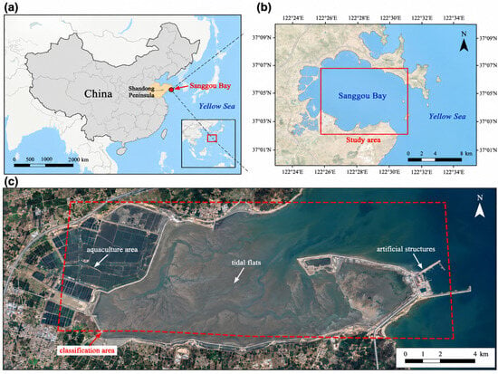
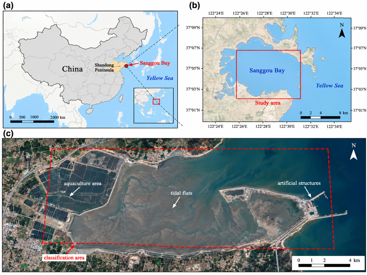
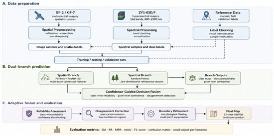
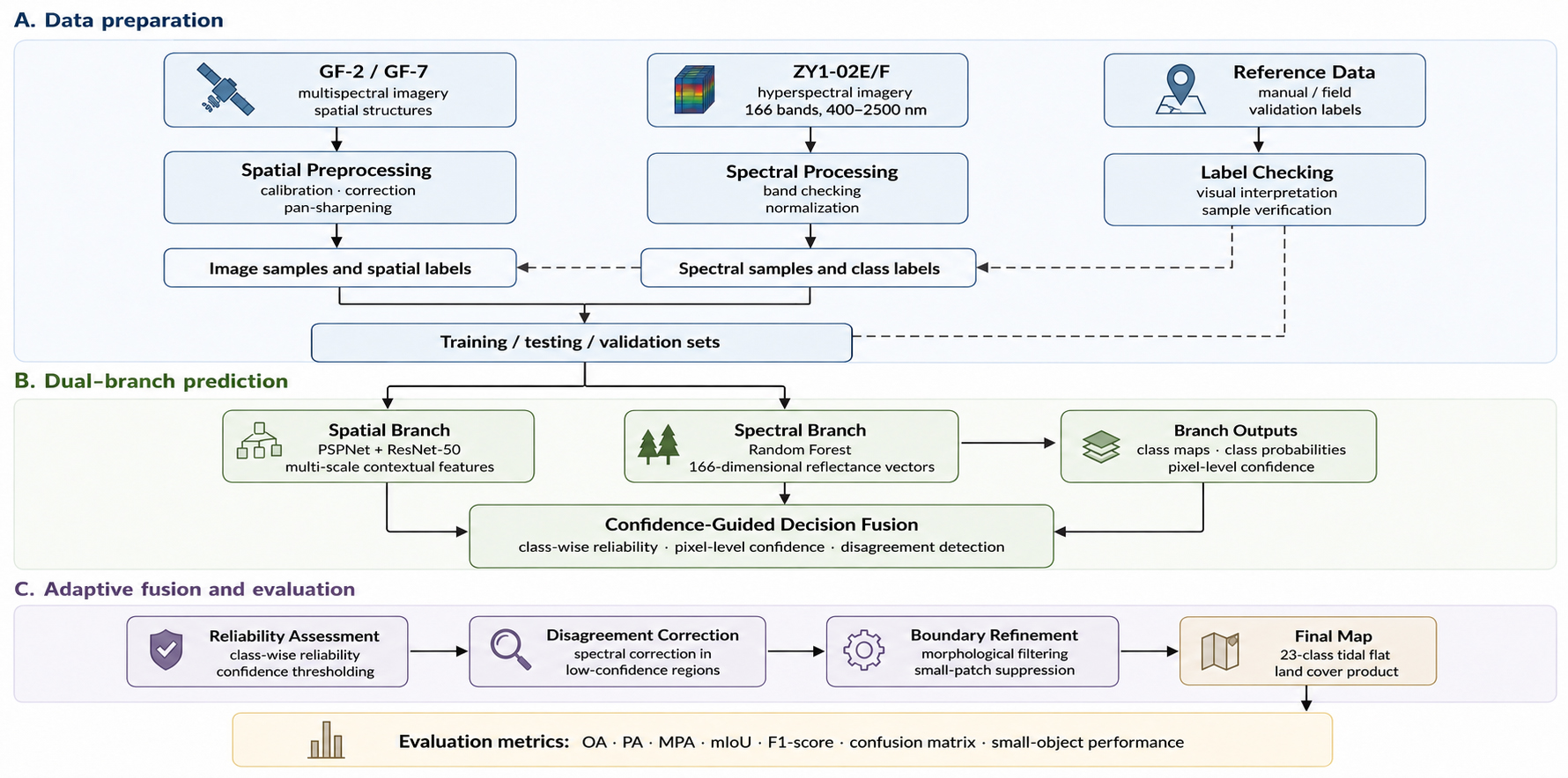
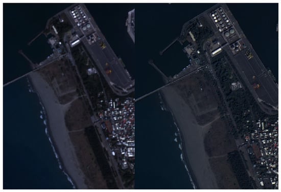
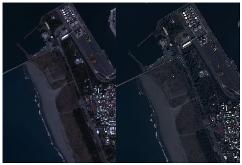
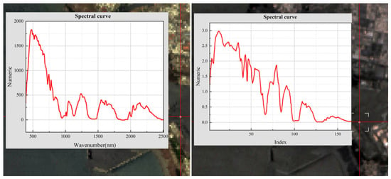
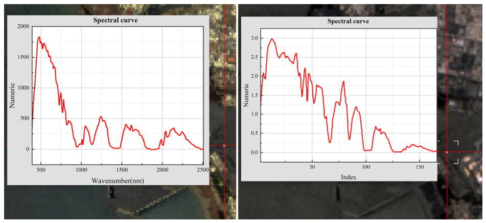
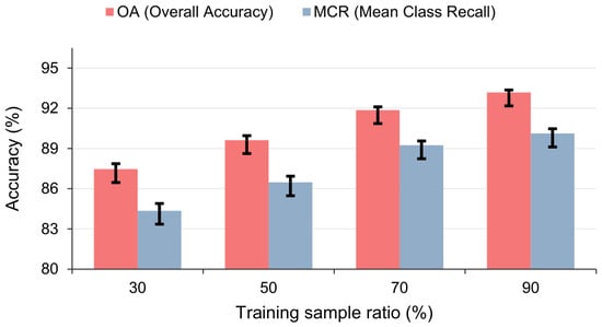
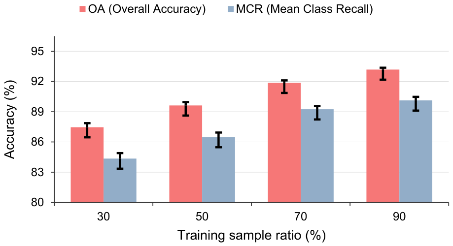
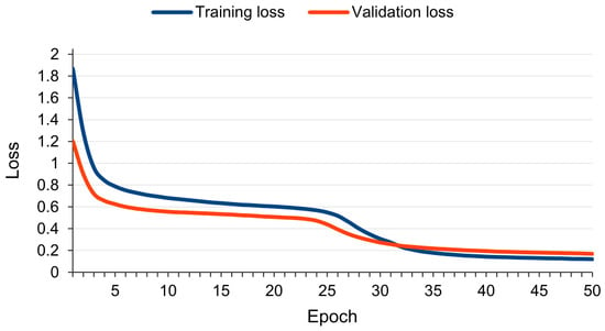
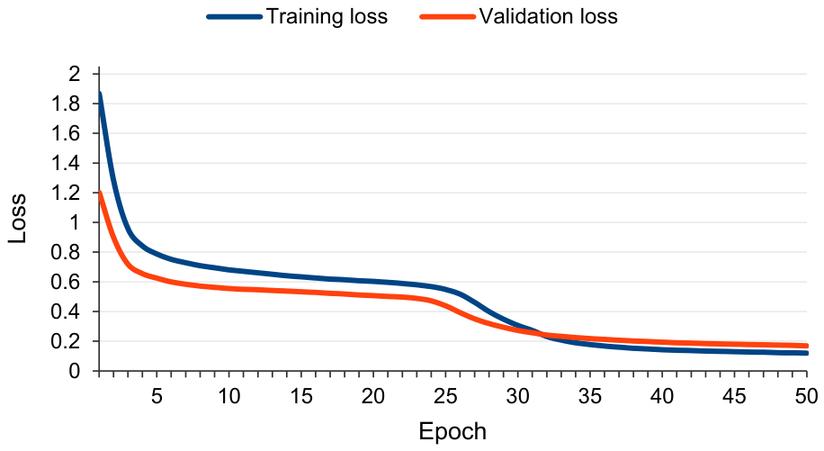
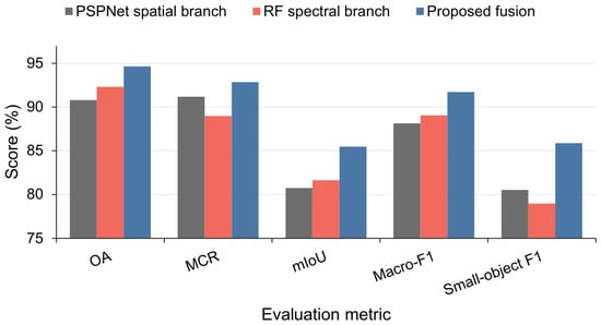
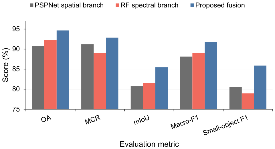
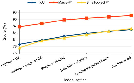
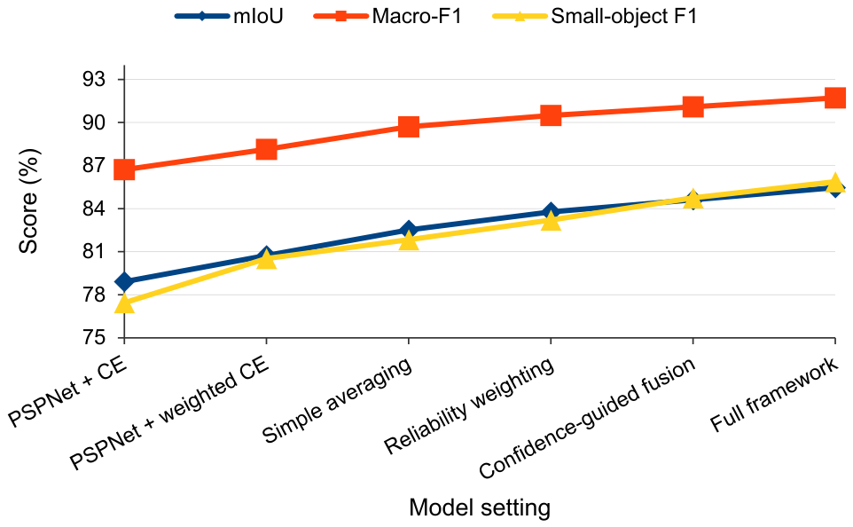
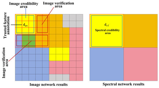
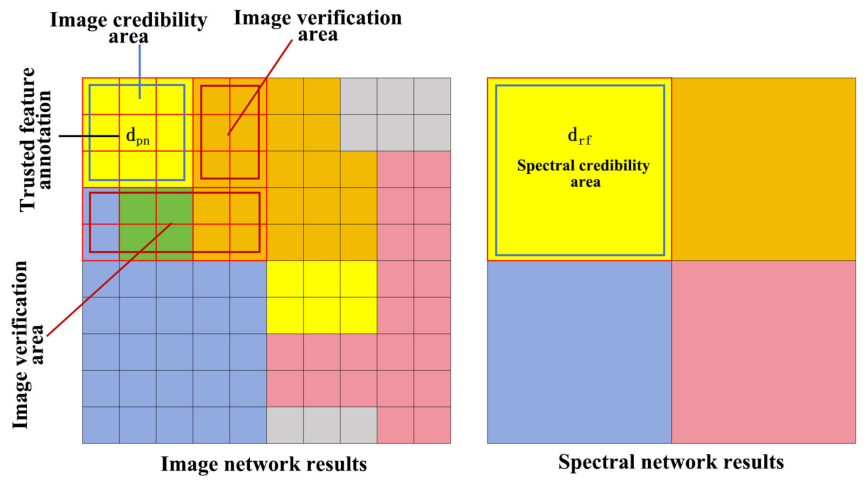
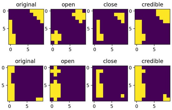
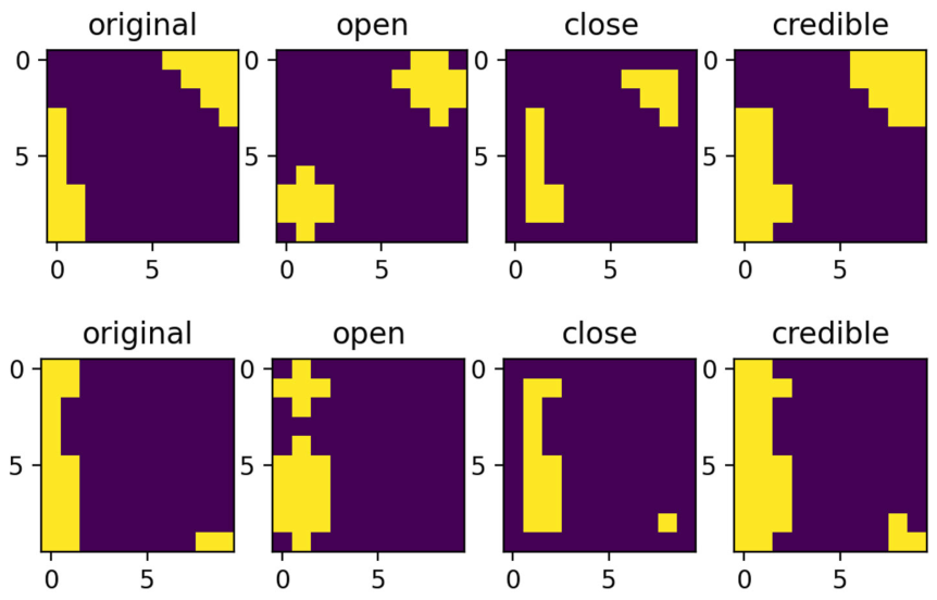
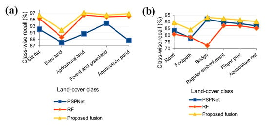
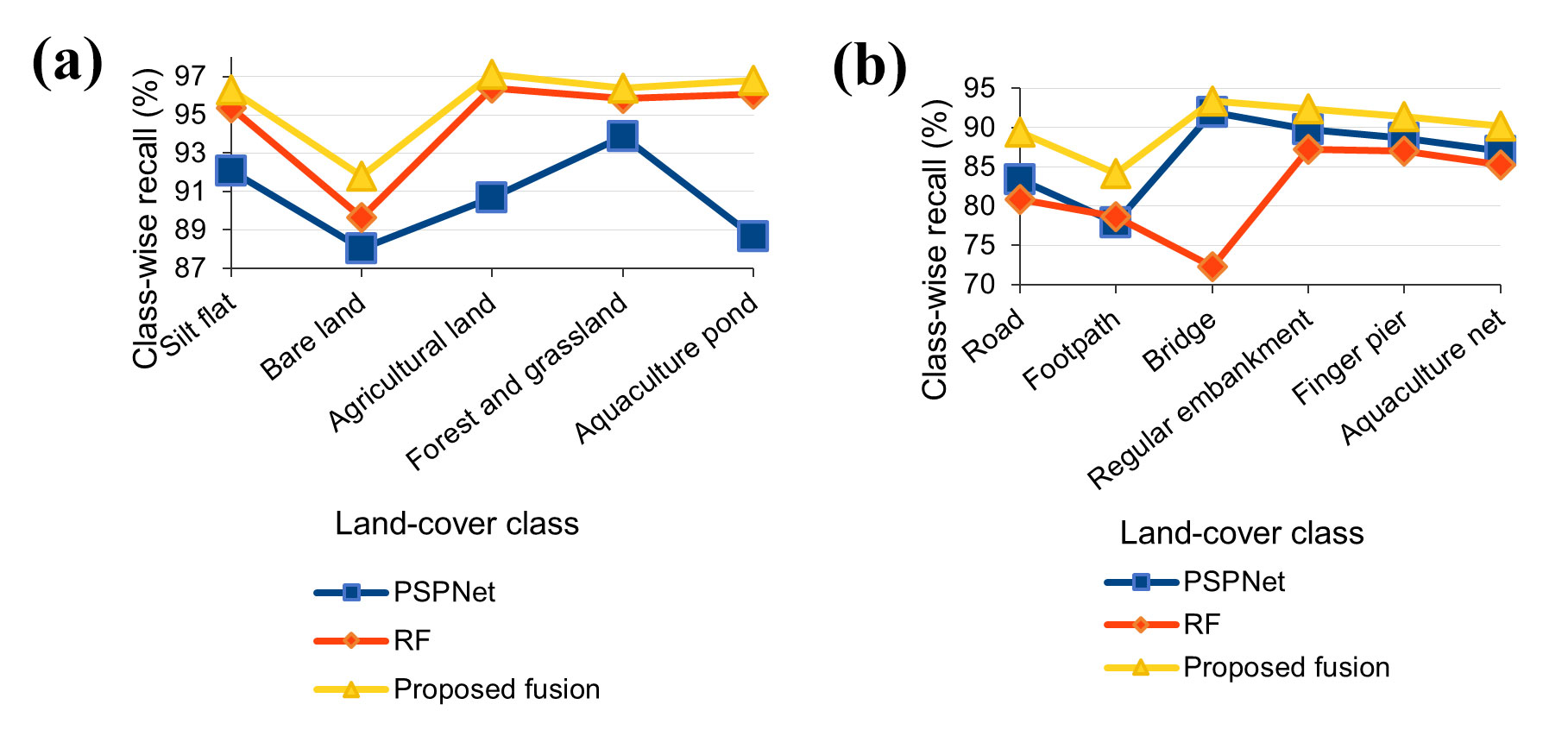
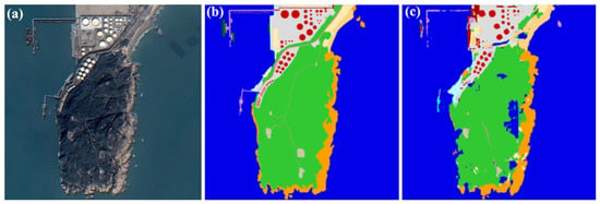
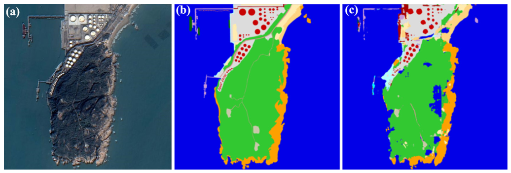
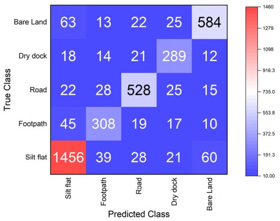
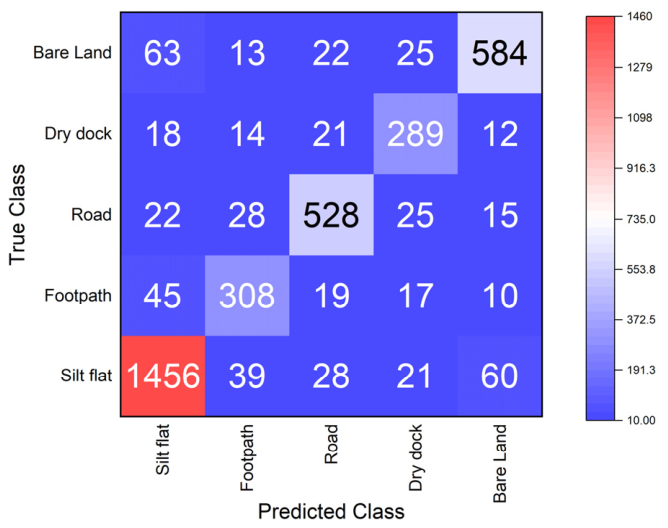

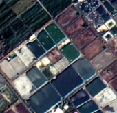
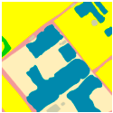
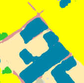
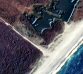
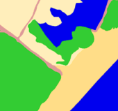
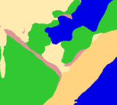
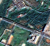
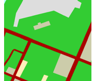
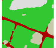


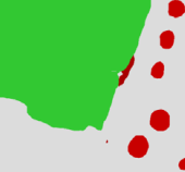

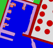
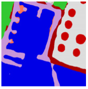
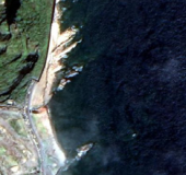
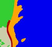



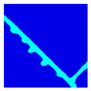

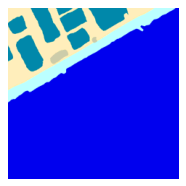
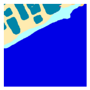
Disclaimer/Publisher’s Note: The statements, opinions and data contained in all publications are solely those of the individual author(s) and contributor(s) and not of MDPI and/or the editor(s). MDPI and/or the editor(s) disclaim responsibility for any injury to people or property resulting from any ideas, methods, instructions or products referred to in the content. |
© 2026 by the authors. Licensee MDPI, Basel, Switzerland. This article is an open access article distributed under the terms and conditions of the Creative Commons Attribution (CC BY) license.