


Abstract
A priority vehicle (PV) can be assisted by learning its own lane choices, coordinating surrounding automated vehicles (AVs), or training both roles. We compare these allocations in a four-lane cellular-automaton model and add an input- and capacity-matched PV-encoder comparison. Policies trained at 90–100% AV fractions and densities of 0.10–0.40 are evaluated on 126 density–composition conditions. Coordinator-only and joint-graph control each have five separately initialized training runs. At 90–100% AV fractions, joint-graph control, coordinator-only control, and reactive yielding achieve mean PV speeds of 2.783, 2.684, and 2.385 cells/step. At 10–75% AVs, outside the training composition range, the corresponding means are 1.958, 1.980, and 2.004. All five selected joint-graph models meet the 0.95 observed background-flow ratio threshold; one coordinator-only model reaches 0.940. Two matched training runs per encoder show no consistent advantage for iterative PV message passing over pooled relations. Lower-AV results cannot distinguish transfer limitations from reduced assisting capacity. The conclusions concern selected policies in an uncalibrated, fixed-length periodic model with one PV and non-yielding human-driven vehicles; they do not establish a general allocation rule or quantitative predictions for real traffic.
1. Introduction
A priority vehicle (PV) can pass a queue by changing lane itself or by using a gap opened by another vehicle. These interventions require different control capabilities. A PV can carry a controller even when few surrounding vehicles can receive a request to yield. A shared coordinator can influence more gaps as the proportion of equipped vehicles increases, but its maneuvers may delay ordinary traffic. This gives rise to an allocation question for reinforcement learning (RL). How do complete allocations of learned lateral control compare, how do policies trained with many assisting vehicles transfer to sparser fleets, and how much background flow is retained?
1.1. Control Targets for Priority Passage
Traffic-control strategies for emergency vehicles span route optimization, signal preemption, lane reservation, and combinations of these interventions [1,2]. These approaches act at different spatial scales and can redistribute delay to ordinary traffic. At intersections, Chen et al. explicitly account for queue spillbacks and recovery of non-priority traffic after preemption [3]. Such infrastructure-level strategies motivate evaluating both priority service and its external effects, but do not replace the link-level question considered here: which vehicles should receive learned lateral control when the road and longitudinal rules are held fixed?
Work on direct PV control has progressed from planning around drivers with different willingness to yield to learning lane changes using vehicle-to-everything information. Buckman et al. modeled semi-cooperative interactions between the emergency vehicle and other drivers [4]. Ding et al. coupled learned emergency-vehicle lane changing with assistance from surrounding vehicles [5]. In both cases it matters which participant chooses the action. An instrumented neighbor can supply information, execute a rule, or act under a learned policy.
A second line of work creates space through surrounding vehicles. Field experiments showed that one controlled vehicle can influence stop-and-go waves on a ring [6]. The Flow framework and decentralized mixed-traffic experiments studied how the available control authority depends on the road and equipped fleet [7,8]. Cooperative lane changes extend this reasoning to lateral actions [9]. For priority passage specifically, Su et al. formulated dynamic queue-jump lanes under partial connectivity [10], while Suo et al. studied corridor clearance with very few assisting vehicles, including a single connected and automated vehicle [11]. The latter study also considers effects on regular traffic and motivates examining low penetration rather than assuming that assistance requires an almost fully automated fleet. Our experiment at low fractions of automated vehicles (AVs) tests transfer of policies trained at high penetration; it does not reproduce training designed specifically for sparse assistance.
Joint control lets both roles adapt. Parada et al. trained emergency and autonomous vehicles to maneuver together [12]. At network scale, EMVLight coordinates routing and signals, and Cheng et al. assign roles to emergency vehicles, regular vehicles, and signals [13,14]. These formulations change the set of possible interventions. In particular, the dynamic role inference of Cheng et al. differs from our comparison of predefined assignments of trainable controllers. A benefit from routing or signal control cannot quantify the incremental value of learning the PV’s lateral decisions on a road segment.
1.2. Information and the Cost to Ordinary Traffic
Optimization and explicit rules are meaningful comparators for learning. Wu et al. coordinated lane pre-clearing and considered disturbance to cooperating vehicles [15]. SafePass includes a cascade-aware penalty in distributed lane-choice utilities to limit disruption from yielding [16]. Experimental traffic-smoothing work also shows that explicit local control can influence collective behavior [17]. For the present question, a learned controller should therefore be compared with an executable yielding rule at the same AV fraction. A second, native-traffic reference is needed to interpret absolute disruption.
Graph models encode relations between vehicles and can aggregate observations from a changing neighborhood. Yang et al. represent changing connectivity in a graph-convolutional soft actor–critic approach to emergency lane clearance [18]. A recent preprint by Su develops hierarchical graph-based learning for queue-jump lanes and corridor formation [19]. These studies motivate relational representations and scalable coordination, rather than establishing that a graph encoder must outperform every alternative. Their reported gains concern their own action spaces, rewards, and traffic environments. Determining what repeated message passing contributes in the present system requires a separate comparison that holds the observed vehicles, relations, and parameter budget approximately fixed.
Multilane cellular automata provide computationally tractable repeated trials of such comparisons; their discrete measurements and relation to physical units are reviewed by Maerivoet and De Moor [20]. Relevant model developments range from stochastic freeway flow and anticipation to delayed starting and lane changes [21,22,23,24]. Emergency-vehicle and corridor-of-life models have already shown how to represent yielding in this setting [25,26]. Testing a control mechanism in a cellular model leaves a separate empirical question. Lichtlé et al. describe the calibration and deployment work needed to transfer a simulated traffic-smoothing controller to road vehicles [27]. In a different vehicle domain, Nowakowski and Wesołowski used operational signals recorded during manned and unmanned operation of the TAERO platform to study controller improvement [28]. Such records illustrate the type of evidence that would complement a simulation of priority passage.
1.3. Study Questions
The related literature establishes several viable mechanisms for priority passage, but results obtained with different simulators, observations, action spaces, and background-traffic objectives do not by themselves rank the allocation of learned control. Our contribution is a within-model comparison, not a claim that cooperative passage, graph-based control, or role-aware learning is new. The five original configurations and four non-learning references are retained, with additional training runs, transfer tests, and a matched encoder comparison.
We make three comparisons under the same longitudinal dynamics and lateral admissibility rules. First, we vary which role learns and test whether its benefit persists when equipment penetration moves outside the training range. Second, we compare two PV encoders given identical graph observations and nearly equal capacity. Third, we assess what an apparent passage gain costs other vehicles by checking background flow for each training lineage and examining motion near the PV. The contribution is a comparison of selected control allocations, an input- and capacity-matched encoder control, and reporting of individual training runs within one traffic model. Comparisons of separately trained joint configurations do not isolate the contribution of the PV alone. We distinguish a descriptive post-training screen from constrained policy optimization [29], and variation between evaluation roads from variation between independent RL trainings [30].
2. Materials and Methods
2.1. Road, Interventions, and References
Four periodic lanes of length cells contain one-cell vehicles, where is the total occupied-site fraction. One is the PV, with a speed limit of 6 cells/step. All other vehicles have limit 5. Of the background vehicles, are designated automated vehicles (AVs). The remainder are human-driven vehicles (HDVs) governed by the same native model, without PV-specific yielding. The AV label makes a vehicle eligible for an external lateral command. Here, f is the nominal AV fraction among background vehicles; the realized fraction is . No physical cell length or time scale is assigned.
At each step the model resolves lateral requests, recomputes leaders in the resulting lanes, and updates longitudinal speeds and positions synchronously. The common stochastic revised stochastic Nishinari–Fukui–Schadschneider (Revised S-NFS)dynamics use anticipation depth 2, delayed starting, and gap-dependent random braking [22,23]. Native lane changes require an incentive and a rear gap and are requested with probability 0.5 when eligible. Learned actions are left, stay, and right. Their full-state simulator mask checks the target lane, occupancy, rear safety, and a one-step cooldown. Individually admissible requests can still conflict at the same target. Conflicting external requests are rejected for both roles, without PV priority, and approved targets are reserved before native changes. External stay suppresses a native change for that step. All speed and braking decisions remain with the common traffic model. Collision avoidance follows from these simulator rules and the full-state mask; it is not a learned safety guarantee. Supplementary Section S1 gives the update equations and parameter values.
Table 1 specifies which role receives learning. An active AV is one within the inclusive window from 10 cells behind to 30 ahead of the PV across all lanes. A single coordinator commands these vehicles. Other background vehicles retain native control. B2 is the composition-matched reactive reference. Every eligible AV up to 30 cells ahead in the PV’s lane requests a move to the adjacent admissible lane maximizing the smaller of its front and rear gaps. Ties alternate by identifier parity. When no request is issued, the vehicle can change lane natively. B1 has an all-HDV background and the same designated PV; it is the native-traffic reference and is evaluated once per density and road. Two additional controls instruct active AVs to stay (N) or to move left whenever admissible (L). All four references use the native PV rule, including its eligible lane-change probability of 0.5 and speed limit of 6, with no special priority in native conflicts. A training lineage denotes one separately initialized run and its selected checkpoint.
Table 1.
Learned role assignments. Counts cover the trainable actor and critic for each role. The coordinator has 355,460 parameters wherever it is learned. A lineage is one separately initialized training run with a selected checkpoint.PV: priority vehicle; AV: automated vehicle; MLP: multilayer perceptron.
2.2. Information and the Matched Encoder Experiment
The local PV multilayer perceptron (MLP) receives 48 of its own and neighborhood features with a 60-cell sensing radius and four global features (PV speed, lane, density, fraction of active graph slots). The graph-augmented PV also observes the features of all active AVs and six directed neighbor slots per node. These encode the nearest active AV ahead and behind in each of the left, current, and right lanes, with relative position, lane, and speed on each edge. Node padding, relation masks, and action masks are explicit. The graph encoder updates node embeddings through three message-passing layers. The coordinator uses a graph actor with three lateral logits per real node and a separate pooled-value head. The original local-versus-graph comparison therefore changes inputs, architecture, and capacity together.
For the matched experiment, receives exactly the same PV, node, edge, global, and mask tensors as . An MLP embeds each source–target pair and its edge features. Masked means pool the node and relation embeddings, with no successive updates to neighboring nodes. The PV has 560 more parameters than in (0.136%). The two encoders share the action space, head dimensions, training budget, worker profile, and two initialization-seed labels. Each PV is jointly trained with a coordinator of the same architecture. The coordinator weights can consequently differ across pairs. Pooling and normalization also differ. The contrast estimates the effect of choosing these two complete encoder designs under matched inputs and nearly matched capacity. Supplementary Section S2 describes individual layers.
2.3. Training, Selection, and Held-Out Evaluation
We used proximal policy optimization (PPO) with RLlib (Ray version 2.56.0) [31,32]. PPO provides a common training framework for the allocation comparison, rather than a new algorithmic contribution; cooperative PPO studies also show the importance of reporting implementation choices [33]. The shared reward at step t is
where p denotes the PV index, is its speed after the transition at step t, and and are the numbers of executed and rejected AV requests, respectively. Counts are unnormalized. Native changes, PV changes, and stay commands have no maneuver penalty. The coordinator clips the likelihood ratio per active AV, then averages over active nodes using a shared time-step advantage. This does not assign a separate causal credit to each vehicle. PV-only policies optimize normalized PV speed. Background throughput is measured after training and does not enter the reward, checkpoint score, or optimization constraint.
All policies trained on the same 12 combinations of and . Each accepted training lineage ran 611 iterations of 16,384 environment steps. The first three seeds per original configuration used 16 rollout workers. The two additional runs for each of A, , and used 64 workers and a learner running on a graphics processing unit (GPU) with the same batch size, minibatch size (256), six epochs, and total budget of 10,010,624 steps. Original training used GPUs and the other original learners used central processing units (CPUs). The shared seed labels identify initialization runs across configurations. They do not turn different trained policies into independent roads.
Validation at selected a checkpoint per lineage. Five candidates (iterations 450, 500, 550, 600, and 611) were assessed on 20 common validation roads using PV speed and a rejected-command screen. The top two within 0.05 cells/step were reassessed on 50 new validation roads. If still within 0.05, the earlier iteration was used. Selected joint models retain both controllers from the same checkpoint. Supplementary Section S3 specifies the screen, hyperparameters, and selected iterations.
The held-out test grid crosses 18 densities (0.05 to 0.90 in steps of 0.05) with seven AV fractions (10, 25, 50, 75, 90, 95, and 100%). Of the 126 cells, 12 reproduce the discrete training conditions, nine interpolate density at the trained AV fractions, and 105 lie outside at least one training range. Density extrapolation covers 11 of 18 values: 0.05 and 0.45–0.90. All four lower AV fractions are outside the training range. Each road starts from an all-HDV placement evolved for 1000 steps. A random vehicle becomes the PV, and AVs are assigned from a common permutation of the remainder. Measurement starts immediately and lasts steps, including the transient after assigning the PV and AV roles. This evaluates a longer passage horizon than the 1000-step training episode; horizon sensitivity was not tested. Evaluation uses deterministic masked argmax actions and stochastic traffic dynamics. Compared controllers share the warmed physical state, PV identity, initial random streams, and AV subset for composition-matched policies. Subsequent random events can diverge after a different action.
2.4. Outcomes and Uncertainty
Our primary outcome is mean PV speed in cells/step. The principal cost measure is background flow, expressed in vehicles per step per lane. With lanes and denoting the speed of vehicle i at time t,
Secondary outcomes are the fraction of steps with , the probability of completing a lap within T, and mean lap time among roads with a completed lap. A horizon-ending episode without a lap counts against completion and has undefined lap time. A lap is completed when accumulated PV displacement increases by L cells; durations between consecutive completions are first averaged within a road. The reported mean then averages successful roads within each model and models equally; it is undefined if any required model has no completed lap.
We average roads within each trained model, then average models with equal weights. Grid summaries give each density–composition cell equal weight; these weights do not represent a real traffic-demand distribution. Supplementary Table S5 separates training conditions, density interpolation, and extrapolation. At lower AV fractions there are 42 roads per trained model. At high fractions the three original models per original family and rules B2, N, and L have 30 roads, and each additional model has 42. Of those panels, 22 road identities overlap (50 in the union). Absolute and paired summaries can therefore use different road supports (Supplementary Table S4). The canonical B1 panel has 42 roads per density. Its intersection with a historical 30-road panel has 22 roads, so revised flow ratios for those policies are not the original 30-road estimates. For each paired speed contrast we first restrict all required policies to the same verified road identities and calculate an equal-model difference on each road. The matched encoder contrast uses only the two additional training seeds per encoder and 42 roads in every cell.
For lineage s and condition c, flow retention is the mean of roadwise ratios over shared roads I with positive reference flow. We use as a chosen descriptive tolerance for each lineage and condition, not an empirically calibrated acceptability threshold. B1 is a native-traffic reference. B2 provides the composition-matched comparison for passage speed. We label a tested configuration as meeting the point screen only when every evaluated lineage meets it in that cell. This convention does not give a safety or noninferiority guarantee.
Pointwise 95% percentile intervals resample road identities 10,000 times (root seed 910019, linear percentiles). The individual-flow calculation derives a deterministic seed from this root and the condition and policy identifiers; the supplied analysis script specifies the convention. Paired contrasts and individual-lineage flow ratios preserve within-road pairing. Absolute speed intervals resample the union of road identities and preserve each model’s availability pattern. All intervals condition on the selected trained models. Counts of intervals above, across, or below zero are descriptive summaries across correlated grid cells, without multiplicity adjustment. Intervals for cells selected after inspection, including the minimum flow ratio, are not selection-adjusted or simultaneous bounds for the grid minimum. Supplementary Table S7 reports individual training-lineage speed means on both their original panels and the common 22-road high-AV panel. These descriptive between-run comparisons address a different source of variation and are not confidence intervals for a new training run. The comparisons are exploratory.
2.5. Local Observations and Decision Diagnostics
To distinguish spatial sampling and restart selection from controller effects, a passive observer collected 20 roads per instrumented model and condition (41,760 of the 116,856 global model–road observations). Local records do not cover all historical models. The example at includes all five lineages. In the 25-cell window centered on the PV (12 cells in either direction and all four lanes), let and denote the count and summed speed of background vehicles. Local density is and local flow is the laboratory-frame snapshot . The denominator includes the PV site. This measure does not count boundary crossings in the moving frame. Four stationary windows of the same width and the entire ring provide spatial controls.
A restart is the first positive PV speed after at least five consecutive observed zero-speed steps. We align observations to that step and distinguish all subsequent observed samples, including renewed stops, from samples with uninterrupted positive PV speed. Right-boundary follow-up is truncated at the observation horizon. Events are averaged within each road, then roads within models, and then models equally. We report the number of events contributing at each lag. Separately, a controller-substitution diagnostic () replaces the learned PV in each of the three lineages with the native rule while retaining its coordinator weights. It covers six densities at 100% AVs, with 22 verified roads shared by the two arms at each density. On those roads we also decompose the speed difference using , where v is the corresponding mean PV speed, is the mean stopped-time fraction, and . Supplementary Section S3 gives the symmetric decomposition and its paired uncertainty.
3. Results
3.1. Fixed-Policy Comparisons Across AV Fractions
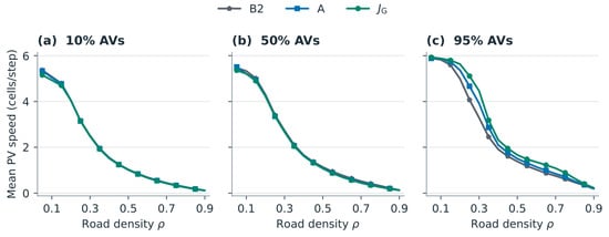
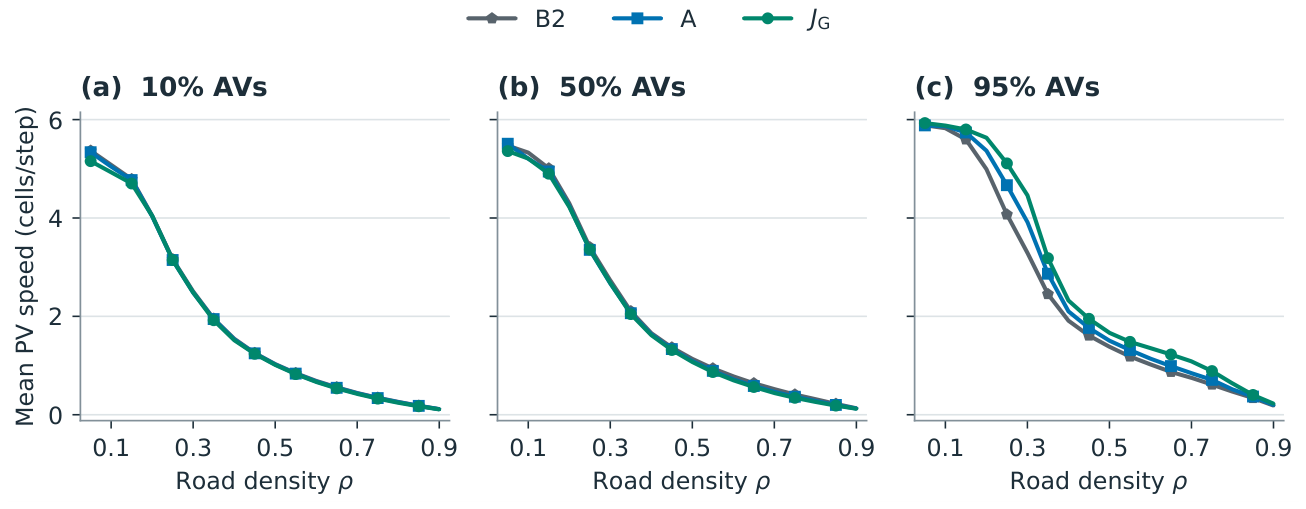
At the three high AV fractions, joint graph control () yielded 2.783 cells/step averaged over 54 density–composition cells, compared with 2.684 for coordinator-only control (A) and 2.385 for reactive yielding (B2). Across the 72 lower-fraction cells, the order reversed: B2 averaged 2.004, A 1.980, and 1.958 (Table 2). These are equal-condition summaries of fixed models trained only at high penetration. They do not locate a critical AV fraction. Separating training conditions, density interpolation, and extrapolation retains this descriptive ordering within each AV regime (Supplementary Table S5). Figure 1 shows how strongly density affects absolute speeds even where the policies are close.
Table 2.
Mean PV speed (cells/step) and minimum observed background-flow ratio across all individual policies or lineages on the full grid. Each speed gives equal weight to the 72 lower-AV or 54 high-AV conditions. Both AV groups include densities outside the training range. B1 is the same native reference in both panels, with a flow ratio identically equal to one. The other minima are descriptive point estimates.
Figure 1.
Absolute mean priority-vehicle (PV) speed across density for B2, A, and at three selected fractions of automated vehicles (AVs). Markers identify simulated conditions. Lines connect adjacent density points, and shading shows pointwise 95% road-bootstrap intervals conditional on the selected models. The seven-fraction display is in Supplementary Figure S1.
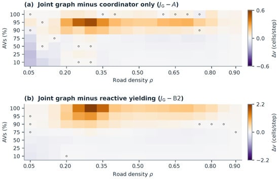
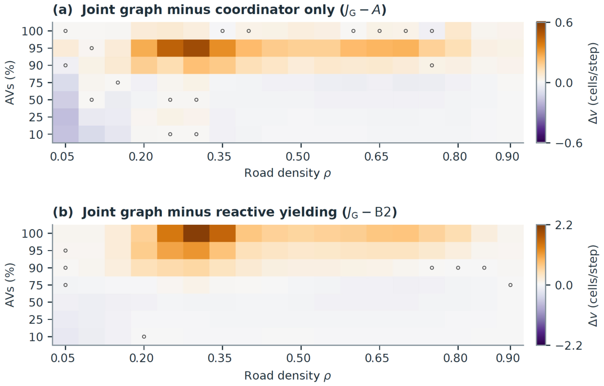
The paired comparisons in Figure 2 display configuration differences against the much larger variation with density. Of the 54 high-AV intervals for minus A, 44 were positive and 10 included zero. Of 72 lower-AV intervals, eight were positive, six included zero, and 58 were negative. Against B2, had 49 positive and five zero-including intervals at high fractions, compared with four positive, three zero-including, and 65 negative intervals below 90%. A alone exceeded B2 in 45 high-AV and four lower-AV intervals and fell below it in three and 60, respectively. The jointly trained system exceeded PV-only learning ( minus ) in all 126 pointwise intervals. This is a comparison of complete trained configurations, not an intervention holding their PV weights fixed.
Figure 2.
Paired PV-speed differences across all 126 conditions. Positive values favor . An open circle marks a pointwise 95% interval including zero. Each panel has a labeled, symmetric color scale in cells/step. Only the 90, 95, and 100% AV fractions occurred in training.
At and , minus A was cells/step (95% interval , 42 roads). At it was on 22 shared roads, and at it was on 22. The relative difference between the high-AV grid averages of and A was 2.36% for the original three lineages and 3.69% for the expanded five. These are configuration-level comparisons: and A have separately trained coordinators, so their difference does not isolate the learned PV. Only the substitution below fixes the coordinator weights. At , the three original and two additional A lineages averaged 2.187 and 1.976. The corresponding means were 2.387 and 2.226. Both additional cohorts were slower at this condition. The original and additional execution profiles differed along with the learned weights and road panels. These cohort means do not isolate an execution-profile effect. Supplementary Table S7 gives all five lineage-level grid means, including a common-road comparison.
The stronger non-learning rule L also provides a direct paired comparator. At high AV fractions, the mean paired gains over L were 0.1149 cells/step for A and 0.2143 for , on the 22 roads common to all included models and the rule. The corresponding pointwise intervals were positive in 33 and 45 of 54 conditions, respectively; A had one negative interval and had none. At lower fractions the paired gains averaged 0.0580 and 0.0354 on 42 common roads (Supplementary Table S6). Thus, the advantage is smaller than against B2, and neither learned configuration dominates both rules throughout the expanded grid.
3.2. Background Flow at the 0.95 Screen
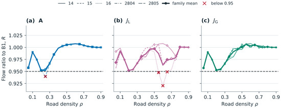
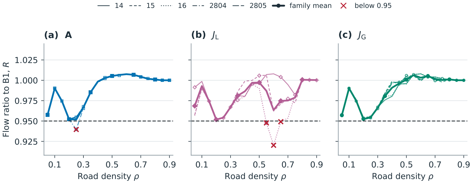
The minimum across all 630 lineage–condition estimates was 0.95172, with a pointwise interval of . The corresponding minimum was 0.95199 across 252 estimates. Both occurred at , . The narrow margin is visible in Figure 3. All 3042 main-grid lineage/rule–condition ratios and their pointwise road-bootstrap intervals are provided in the accompanying analysis materials. These intervals describe fixed-policy road comparisons, not simultaneous or selection-adjusted inference on the minimum across the grid.
Figure 3.
Individual training lineages and equal-lineage means of the background-flow ratio at 100% AVs. Thin lines with open markers show separate trainings. Legend suffixes 14, 15, and 16 denote seeds 20260914–16, and 2804 and 2805 denote 2026102804–05. Bold lines are family means. Crosses mark individual estimates below the horizontal 0.95 screen. Ordinates are identical in all three panels. Historical lineages use 22 matched roads and additional lineages use 42; Table 3 supplies intervals for every failed point estimate.
Table 3 lists every point estimate below the screen. For A at , averaging the five lineages yields 0.95183 and hides the 0.93960 attained by one model. For , all three failures belong to one trained policy. The historical and L ratios now use the 22-road intersection with the canonical B1 panel; their additional threshold crossings therefore reflect a changed paired support, not new training runs. All seven intervals in the table overlap 0.95. A failed point screen and uncertainty about the underlying fixed-policy mean therefore coexist. Requiring both a positive paired speed interval against B2 and all tested lineages to clear the flow screen left 49 of 54 high-AV cells for and 44 for A, compared with just four of 72 lower-AV cells for each. B2 itself retained at least 0.9755 of native flow across the grid.
Table 3.
All observed violations of the individual background-flow point screen. The bootstrap interval resamples matched roads for the named lineage or rule. The family column gives the equal-lineage mean in that cell.
3.3. Matching PV Information and Capacity Changes the Architectural Interpretation
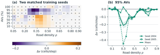
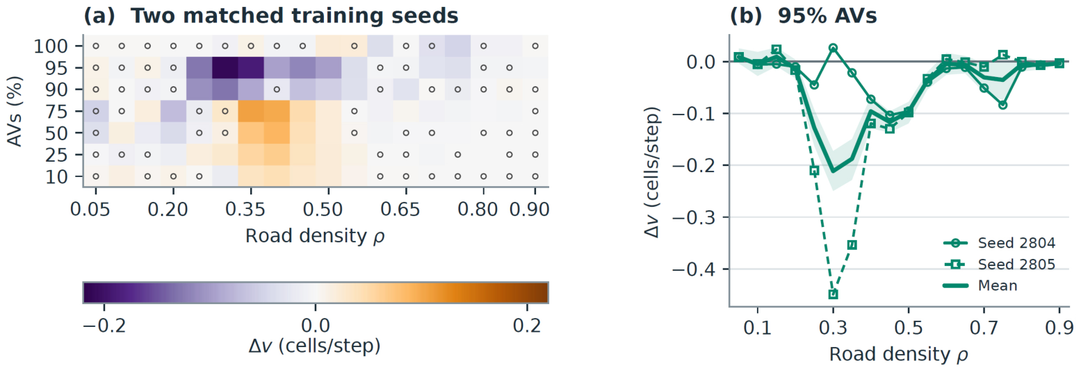
Figure 4 compares the two additional lineages only with the two matched lineages. The minus interval was positive in 25 conditions, included zero in 67, and was negative in 34. At 90% and 95% AVs, seven and ten intervals, respectively, favored and none favored . At , the paired differences for 50, 95, and 100% AVs were , , and cells/step. All three estimates use 42 roads. Subtracting the two high-fraction averages in Table 2 would mix different training cohorts. The matched results provide no consistent advantage for iterative PV message passing over pooled relations.
Figure 4.
Matched PV encoder contrasts ( minus ). Panel (a) shows two equally weighted seed pairs on 42 common roads per cell. Open circles mark intervals including zero. In (b), lines with open markers show the two seed-specific contrasts at 95% AVs. The bold mean and its shaded interval describe road uncertainty for those fixed pairs.
3.4. When the Learned Local PV Increases Stopped Time
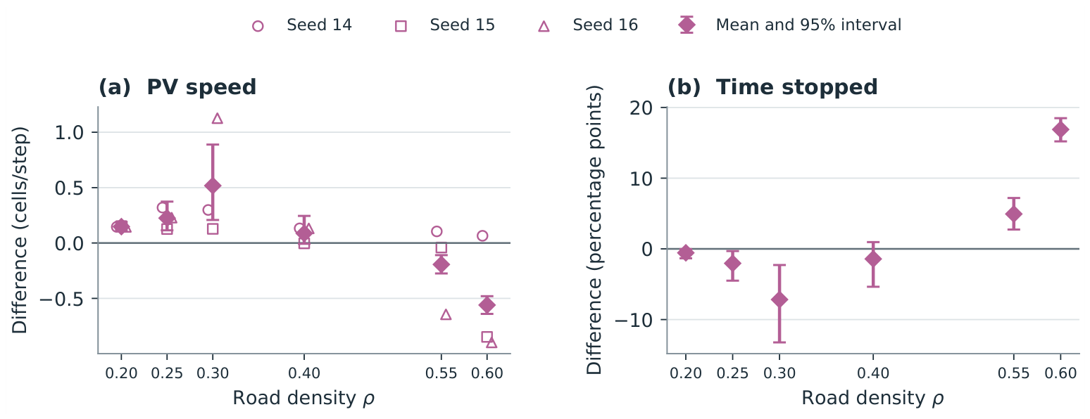
For minus A the high-AV grid contained 12 positive, 10 zero-including, and 32 negative intervals. At , was stopped for 0.694 of steps, compared with 0.327 for A and 0.332 for . Their mean speeds were 0.661, 1.538, and 1.538 cells/step, respectively. Dividing each mean speed by its moving-time fraction gave 2.162, 2.288, and 2.304 cells/step. Thus, in this cell the largest separation was in time spent stopped. Only 31 of 90 model–road observations completed a lap, versus 174 of 174 for A and for . Reporting only the conditional lap time (777 steps) would omit most of its observed runs. At a density of 0.90, no tested main-grid policy completed a lap within 2000 steps.
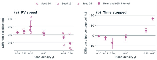
The fixed-coordinator substitution in Figure 5 tests whether the learned local PV contributes to this deficit. Relative to replacing it with the native PV, the learned PV increased speed at densities of 0.20, 0.25, and 0.30. The interval included zero at 0.40. At 0.55 and 0.60 the differences were and cells/step. The same substitution can therefore help or hinder, depending on density, even when coordinator weights are fixed. At a density of 0.60, the learned PV was stopped for 63.65% of the time, compared with 46.77% for the native PV under the same three coordinators. The paired increase was 16.89 percentage points . Of the cells/step difference, the symmetric decomposition assigned to the change in the stopped-time fraction and to the change in speed while moving. These components describe how the speed difference arose numerically. The paired records contain no stepwise PV/AV request and rejection histories for these high-AV comparisons, so the frequency of conflicting commands cannot be inferred from them.
Figure 5.
Learned local PV minus native PV with the same three coordinators at 100% AVs. (a) Speed differences by lineage (open symbols, displaced horizontally for visibility) and their equal-weight mean (diamonds). (b) Difference in the proportion of time stopped, in percentage points. Bars in both panels show pointwise 95% intervals on the same 22 paired roads per density.
3.5. Whole-Ring Throughput and Motion near the PV
The PV contributes at most vehicles/(step·lane) directly to whole-ring flow. Its indirect influence on surrounding vehicles can be larger. Table 4 shows why the spatial reference matters. At the moving window was more crowded and carried less flow than a stationary window or the whole ring. A similar difference occurred in native B1. A window following the PV spends more time where the PV is delayed, so its difference from a fixed window cannot by itself be attributed to the controller.
Table 4.
Background density (vehicles/site) and laboratory-frame snapshot flow (vehicles per step per lane) at and 50% AVs. Each spatial domain averages the same 20 instrumented roads per model. B1 is the canonical all-HDV reference. The stationary window shown is centered at the origin.
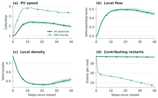
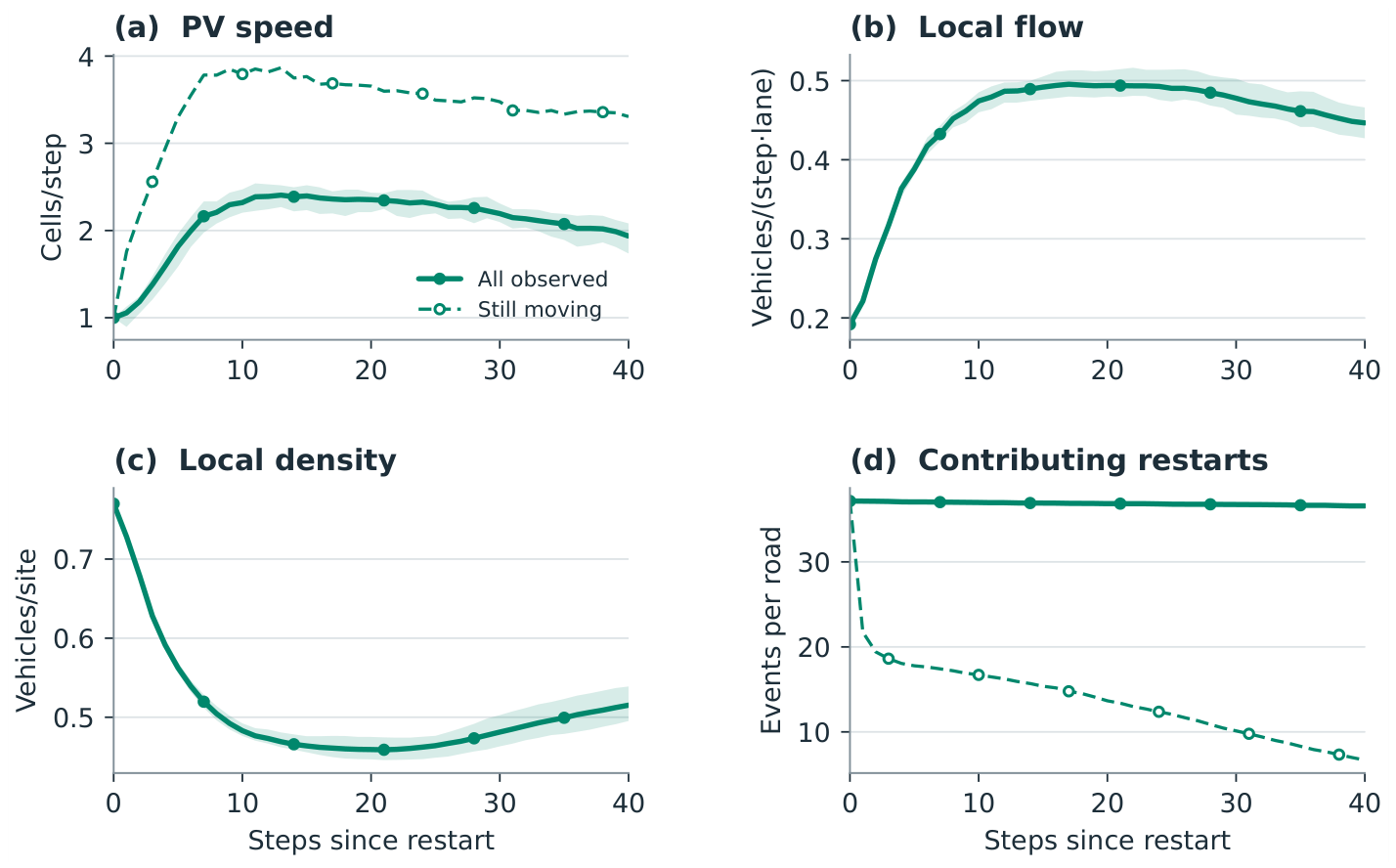
After a qualifying restart, the mean speed over all observed follow-up rose from 1.00 at lag 0 to 2.35 cells/step at lag 20, then fell to 1.94 by lag 40 (Figure 6). Local flow changed from 0.192 to 0.494 to 0.447, while background density fell from 0.770 to 0.459 and then rose to 0.515. Restricting the same calculation to uninterrupted motion gave a mean PV speed of 3.31 at lag 40. An average of only 6.68 such events per road still contributed, versus 36.59 in all follow-up. All 20 roads per model still supplied at least one event in both selections. These observations distinguish acceleration after a stop from selection for longer movement. They do not establish a universal plateau in local flow.
Figure 6.
after restarts at . Panel (a) compares all observed follow-up with events that remained in motion until that lag. Panels (b,c) show moving-window background flow and density for all observed follow-up. Panel (d) shows mean contributing event counts per road. Curves average events within roads and give the five trained models equal weight. Shading in (a–c) spans the five all-follow-up model means and describes between-lineage spread. PV: priority vehicle.
4. Discussion
4.1. Role Allocation and Transfer of the Selected Policies
The full-grid means were 1.852 cells/step for and 1.851 for , compared with 1.870 for native B1. These descriptive means do not establish a paired loss in every condition. Limited optimization, checkpoint selection, density extrapolation, the longer test horizon, and suppression of native lane changes by explicit PV actions are possible explanations; none of these are isolated here. Coordinated configurations had substantially higher speeds at high AV fractions, but comparing separately trained coordinators cannot isolate the PV contribution. At high AV fractions often exceeded A and B2. At lower fractions B2 usually exceeded both. A plausible explanation is that the explicit rule can act whenever a yielding opportunity arises, whereas the learned coordinators encountered predominantly large active sets in training. The study changes composition during evaluation and does not retrain policies at lower fractions. The test grid also extrapolates beyond the training density range at and . It cannot distinguish a limit on available control authority from a limit on transfer to unfamiliar traffic.
The matched encoder results narrow the interpretation of the original comparison. Richer observation inputs and markedly different model sizes accompanied the original change from local to graph-augmented PV control. Once both PVs saw the same active vehicles and relations, paired speed differences changed sign across the grid. A pooled encoder retained competitive performance even though it never propagated an updated node state to a second neighbor. Both systems still used a learned graph coordinator and different jointly optimized weights. Two encoder pairs provide limited information about the variability expected from new training runs.
4.2. Traffic Costs and Local Mechanisms
An operational comparison needs both a feasible non-learning controller and a measure of its effects on other road users. B2 is a feasible composition-matched reference, not the strongest possible heuristic. At high AV fractions, the left-if-safe rule L has a higher grid mean than B2 (2.570 vs. 2.385 cells/step), but its minimum flow ratio is 0.9343. No heuristic was tuned, and these summaries do not establish an optimized speed–flow Pareto frontier. The chosen native-flow screen permits an observed mean reduction of up to 5% and says little about its distribution across individual vehicles. The learning reward discourages AV maneuvers, especially rejected requests, without pricing background travel or delay. Consequently, meeting the screen is an observed post-training outcome, and a speed improvement can coincide with a screen failure. At high density, the fixed-coordinator experiment identifies one circumstance in which changing only the PV policy alters passage. The symmetric decomposition at a density of 0.60 assigns most of the speed loss to the greater fraction of time at rest; it does not determine whether individual stops were longer or more frequent. Moves into lanes with unfavorable downstream conditions and requests by both roles for the same target are two possible explanations for that extra stopped time. A physically admissible target need not improve subsequent progress. Testing them requires recording proposed and executed actions separately.
Local and global flow answer different questions. Whole-ring flow measures the time-averaged displacement of all background vehicles per road site. A window moving with one PV follows the traffic the PV experiences and changes its membership as the PV moves. In the restart example, local traffic first discharged, then included more vehicles at rest. Keeping only long, uninterrupted runs raised the apparent late speed and sharply reduced event support. A density-invariant discharge plateau or a distinct third phase cannot be diagnosed from this conditional profile alone. One PV on a ring of fixed length also leaves the scaling of its influence with road length unresolved.
4.3. Limits and Next Tests
The idealized ring excludes intersections, entry and exit flows, sensing failures, and physical braking distances. HDVs have no PV-specific yielding response, and the PV/background speed limits are fixed at 6/5 cells per step. Allowing human yielding or changing this ratio could alter both learned and rule-based outcomes; the direction of the ranking change is not established. The simulator’s action mask has access to the complete relevant state. Assigning a cell length and step duration would give and per lane, but this unit conversion is not empirical calibration [20]. Physical transfer would require choosing these scales and the behavioral parameters jointly against measured speed–headway and queue-discharge curves. Lane-change rates and background delay could then be checked on independent trajectories from another location or time period. The present values quantify mechanisms within the simulator and are not calibrated predictions of emergency response times or real-road capacity.
Road-bootstrap intervals condition on the selected weights; the two to five training runs per family and different execution cohorts do not provide a calibrated uncertainty estimate for a newly trained policy. The reported interval counts are descriptive. Checkpoint selection used one high-AV condition and only iterations 450–611; 11 of 21 selections were at the lower boundary. Earlier checkpoints or a wider validation grid could change the result. Retained log segments and selected weights do not reconstruct complete environment and sampler states.
Several targeted experiments would distinguish the remaining explanations. Training at the four lower AV fractions under the same transition budget would help distinguish transfer limitations from limited assisting capacity. A native-PV substitution with each fixed coordinator would test the PV contribution beyond the existing diagnostic. Sensitivity to HDV yielding and the 6/5 speed-limit ratio would test assumptions shared by all controllers. Logging requests, target cells, executions, and subsequent stops for paired local-PV and native-PV episodes would test the conflict hypothesis. To address background-flow effects during learning rather than only after it, a further experiment should compare the present reward with an explicitly justified flow constraint or background-delay term under the same training budget [29]. Finally, runs with one PV at several ring lengths, keeping density, AV fraction, and the diagnostic window width fixed, would separate changing spatial exposure from a road-wide traffic effect. For this last test, both a fixed-step and a lap-scaled measurement horizon are needed because changing length also changes the opportunity to complete a lap. None of these comparisons is available in the present data.
5. Conclusions
In this four-lane periodic model, the selected high-penetration-trained policies performed differently across AV fractions. Joint graph control had higher mean PV speed than coordinator-only control and the specified reactive yielding rule at 90–100% AVs; yielding had the highest of these three means at 10–75%. The latter comparison combines reduced assisting capacity with transfer beyond training and does not identify a generally preferable allocation. All five selected joint-graph runs met the observed background-flow point screen, while one coordinator-only run did not. Matching PV observations and capacity yielded no consistent advantage for the iterative encoder in the two matched training pairs. The evidence supports configuration comparisons and individual-run reporting within this uncalibrated, fixed-length model; it does not establish safety, noninferiority, or performance under retraining.
Supplementary Materials
The following supporting information can be downloaded at https://www.mdpi.com/article/10.3390/app162111028/s1. Section S1. Cellular automaton and maneuver execution; Section S2. Observation and encoder specification; Section S3. Training, selection, and coverage; Section S4. Additional outcome and training figures; Table S1. Shared traffic and local-control parameters; Table S2. Ordered local feature groups, using zero-based indices; Table S3. Selected iteration by policy family and full initialization seed; Table S4. Archived road support; Table S5. Descriptive mean PV speeds (cells/step) by relation to training conditions; Table S6. Paired PV-speed differences against L; Table S7. PV speed by training lineage (cells/step); Figure S1. Mean PV speed by global density and AV fraction; Figure S2. Fraction of measured steps for which the PV was stopped; Figure S3. Probability of at least one completed lap during 2000 measured steps; Figure S4. Absolute background flow, excluding the PV, in vehicles per step per lane; Figure S5. Retained iteration-level training histories. The accompanying data and scripts contain the plotted values, lineage-level flow intervals, and the additional paired-rule and per-lineage summaries in Tables S6 and S7.
Author Contributions
Conceptualization and methodology, M.S.T. and N.V.B. Software, validation, formal analysis, investigation, data curation, visualization, and writing—original draft, M.S.T. Supervision, project administration, funding acquisition, and writing—review and editing, N.V.B. All authors have read and agreed to the published version of the manuscript.
Funding
This research was supported by the Ministry of Transport of the Russian Federation under State Assignment No. 103-00001-26-00, code 4, dated 15 January 2026.
Institutional Review Board Statement
Not applicable. The work uses a computational traffic model and involves no human participants or animals.
Informed Consent Statement
Not applicable.
Data Availability Statement
The revision’s per-road evaluation records, local aggregates, retained training metrics, selected weights for all 21 models (31 policy states), analysis scripts, and model-source references are available in release v1.1.0 at https://github.com/TovarnovM/traffic_pv_article/releases/tag/v1.1.0 (accessed on 4 November 2026). The numeric policy snapshots do not contain optimizer or simulator states. Raw local trajectories and complete training-state histories are not included. The saved-data calculations for the additional summaries in Supplementary Tables S6 and S7 are supplied in the analysis companion accompanying this revision.
Acknowledgments
During the preparation of this manuscript, the authors used ChatGPT (GPT-6 Luna, https://chatgpt.com/overview/, accessed on 4 November 2026), Prism (https://openai.com/prism/, accessed on 4 November 2026), and Codex (https://openai.com/codex/, accessed on 4 November 2026) (OpenAI) to assist with English-language drafting and editing, translation, LATEX formatting, and consistency checks of the manuscript and numerical summaries against archived simulation outputs. The authors reviewed and edited the material prepared with assistance from these tools and take full responsibility for the final content of the manuscript.
Conflicts of Interest
The authors declare no conflicts of interest.
References
- Yu, W.; Bai, W.; Luan, W.; Qi, L. State-of-the-Art Review on Traffic Control Strategies for Emergency Vehicles. IEEE Access 2022, 10, 109729–109742. [Google Scholar] [CrossRef] [Scilit]
- Hao, Z.; Wang, Y.; Yang, X. Every Second Counts: A Comprehensive Review of Route Optimization and Priority Control for Urban Emergency Vehicles. Sustainability 2024, 16, 2917. [Google Scholar] [CrossRef] [Scilit]
- Chen, Y.-Y.; Wang, J.-Y.; Lo, S.-C.; Sung, W.-T. An emergency vehicle traffic signal preemption system considering queue spillbacks along routes and negative impacts on non-priority traffic. IET Intell. Transp. Syst. 2024, 18, 1385–1395. [Google Scholar] [CrossRef] [Scilit]
- Buckman, N.; Schwarting, W.; Karaman, S.; Rus, D. Semi-Cooperative Control for Autonomous Emergency Vehicles. In Proceedings of the 2021 IEEE/RSJ International Conference on Intelligent Robots and Systems (IROS), Prague, Czech Republic, 27 September–1 October 2021; IEEE: Piscataway, NJ, USA, 2021; pp. 7052–7059. [Google Scholar] [CrossRef] [Scilit]
- Ding, C.; Ho, I.W.H.; Chung, E.; Fan, T. V2X and Deep Reinforcement Learning-Aided Mobility-Aware Lane Changing for Emergency Vehicle Preemption in Connected Autonomous Transport Systems. IEEE Trans. Intell. Transp. Syst. 2024, 25, 7281–7293. [Google Scholar] [CrossRef] [Scilit]
- Stern, R.E.; Cui, S.; Delle Monache, M.L.; Bhadani, R.; Bunting, M.; Churchill, M.; Hamilton, N.; Haulcy, R.; Pohlmann, H.; Wu, F.; et al. Dissipation of stop-and-go waves via control of autonomous vehicles: Field experiments. Transp. Res. Part C 2018, 89, 205–221. [Google Scholar] [CrossRef] [Scilit]
- Wu, C.; Kreidieh, A.R.; Parvate, K.; Vinitsky, E.; Bayen, A.M. Flow: A modular learning framework for mixed autonomy traffic. IEEE Trans. Robot. 2022, 38, 1270–1286. [Google Scholar] [CrossRef] [Scilit]
- Vinitsky, E.; Lichtlé, N.; Parvate, K.; Bayen, A.M. Optimizing mixed autonomy traffic flow with decentralized autonomous vehicles and multi-agent reinforcement learning. ACM Trans. Cyber-Phys. Syst. 2023, 7, 13. [Google Scholar] [CrossRef] [Scilit]
- Zhou, W.; Chen, D.; Yan, J.; Li, Z.; Yin, H.; Ge, W. Multi-agent reinforcement learning for cooperative lane changing of connected and autonomous vehicles in mixed traffic. Auton. Intell. Syst. 2022, 2, 5. [Google Scholar] [CrossRef] [Scilit]
- Su, H.; Shi, K.; Chow, J.Y.J.; Jin, L. Dynamic queue-jump lane for emergency vehicles under partially connected settings: A multi-agent deep reinforcement learning approach. arXiv 2020, arXiv:2003.01025. [Google Scholar] [CrossRef] [Scilit]
- Suo, D.; Jayawardana, V.; Wu, C. Model-Free Learning of Corridor Clearance: A Near-Term Deployment Perspective. IEEE Trans. Intell. Transp. Syst. 2024, 25, 4833–4848. [Google Scholar] [CrossRef] [Scilit]
- Parada, L.; Candela, E.; Marques, L.; Angeloudis, P. Safe and efficient manoeuvring for emergency vehicles in autonomous traffic using multi-agent proximal policy optimisation. Transp. A 2025, 21, 2246586. [Google Scholar] [CrossRef] [Scilit]
- Su, H.; Zhong, Y.D.; Chow, J.Y.J.; Dey, B.; Jin, L. EMVLight: A multi-agent reinforcement learning framework for an emergency vehicle decentralized routing and traffic signal control system. Transp. Res. Part C Emerg. Technol. 2023, 146, 103955. [Google Scholar] [CrossRef] [Scilit]
- Cheng, M.; Chen, H.; Li, Z.; Wang, J.; Wang, S. Role-aware Multi-agent Reinforcement Learning for Coordinated Emergency Traffic Control. Adv. Neural Inf. Process. Syst. 2025, 38, 154168–154190. [Google Scholar] [CrossRef] [Scilit]
- Wu, J.; Kulcsár, B.; Ahn, S.; Qu, X. Emergency vehicle lane pre-clearing: From microscopic cooperation to routing decision making. Transp. Res. Part B Methodol. 2020, 141, 223–239. [Google Scholar] [CrossRef] [Scilit]
- Osho, O.; Chakraborty, S.; Das, S.K. SafePass: Efficient emergency vehicle passage with minimal disruption to traffic flow. Transp. Res. Interdiscip. Perspect. 2026, 37, 102011. [Google Scholar] [CrossRef] [Scilit]
- Hayat, A.; Alanqary, A.; Bhadani, R.; Denaro, C.; Weightman, R.J.; Xiang, S.; Lee, J.W.; Bunting, M.; Gollakota, A.; Nice, M.W.; et al. Traffic Smoothing Using Explicit Local Controllers: Experimental Evidence for Dissipating Stop-and-go Waves with a Single Automated Vehicle in Dense Traffic. IEEE Control Syst. 2025, 45, 95–110. [Google Scholar] [CrossRef] [Scilit]
- Yang, X.; Li, M.; Zhang, K.; Zhao, Q.; Guo, Y. Lane clearance for emergency vehicle passage in connected and automated environment: A graph convolutional soft actor-critic method. Expert Syst. Appl. 2025, 290, 128423. [Google Scholar] [CrossRef] [Scilit]
- Su, H. Hierarchical GNN-Based Multi-Agent Learning for Dynamic Queue-Jump Lane and Emergency Vehicle Corridor Formation. arXiv 2026, arXiv:2601.04177. [Google Scholar] [CrossRef] [Scilit]
- Maerivoet, S.; De Moor, B. Cellular automata models of road traffic. Phys. Rep. 2005, 419, 1–64. [Google Scholar] [CrossRef] [Scilit]
- Nagel, K.; Schreckenberg, M. A cellular automaton model for freeway traffic. J. Phys. I 1992, 2, 2221–2229. [Google Scholar] [CrossRef] [Scilit]
- Nishinari, K.; Fukui, M.; Schadschneider, A. A stochastic cellular automaton model for traffic flow with multiple metastable states. J. Phys. A Math. Gen. 2004, 37, 3101–3110. [Google Scholar] [CrossRef] [Scilit]
- Kokubo, S.; Tanimoto, J.; Hagishima, A. A new cellular automata model including a decelerating damping effect to reproduce Kerner’s three-phase theory. Phys. A Stat. Mech. Its Appl. 2011, 390, 561–568. [Google Scholar] [CrossRef] [Scilit]
- Kukida, S.; Tanimoto, J.; Hagishima, A. Analysis of the influence of lane changing on traffic-flow dynamics based on the cellular automaton model. Int. J. Mod. Phys. C 2011, 22, 271–281. [Google Scholar] [CrossRef] [Scilit]
- Zhao, H.T.; Zhao, X.; Lu, J.C.; Xin, L.Y. Cellular automata model for Urban Road traffic flow Considering Internet of Vehicles and emergency vehicles. J. Comput. Sci. 2020, 47, 101221. [Google Scholar] [CrossRef] [Scilit]
- Małecki, K.; Kamiński, M.; Wąs, J. A multi-cell Cellular Automata model of traffic flow with emergency vehicles: Effect of a corridor of life and drivers’ behaviour. J. Comput. Sci. 2022, 61, 101628. [Google Scholar] [CrossRef] [Scilit]
- Lichtlé, N.; Vinitsky, E.; Nice, M.; Bhadani, R.; Bunting, M.; Wu, F.; Piccoli, B.; Seibold, B.; Work, D.B.; Lee, J.W.; et al. From Sim to Real: A Pipeline for Training and Deploying Traffic Smoothing Cruise Controllers. IEEE Trans. Robot. 2024, 40, 4490–4505. [Google Scholar] [CrossRef] [Scilit]
- Nowakowski, M.; Wesołowski, M. Operational Signatures for Control Algorithms Improvement in Optionally Manned Vehicle TAERO. In Proceedings of the 2025 International Conference on Military Technologies (ICMT), Brno, Czech Republic, 27–30 May 2025; IEEE: Piscataway, NJ, USA, 2025; pp. 1–5. [Google Scholar] [CrossRef] [Scilit]
- Achiam, J.; Held, D.; Tamar, A.; Abbeel, P. Constrained Policy Optimization. In Proceedings of the 34th International Conference on Machine Learning, Sydney, Australia, 6–11 August 2017; PMLR: Cambridge, MA, USA, 2017; Volume 70, pp. 22–31. [Google Scholar]
- Agarwal, R.; Schwarzer, M.; Castro, P.S.; Courville, A.C.; Bellemare, M.G. Deep Reinforcement Learning at the Edge of the Statistical Precipice. In Advances in Neural Information Processing Systems; Curran Associates, Inc.: Red Hook, NY, USA, 2021; Volume 34, pp. 29304–29320. [Google Scholar]
- Schulman, J.; Wolski, F.; Dhariwal, P.; Radford, A.; Klimov, O. Proximal policy optimization algorithms. arXiv 2017, arXiv:1707.06347. [Google Scholar] [CrossRef] [Scilit]
- Liang, E.; Liaw, R.; Nishihara, R.; Moritz, P.; Fox, R.; Goldberg, K.; Gonzalez, J.E.; Jordan, M.I.; Stoica, I. RLlib: Abstractions for distributed reinforcement learning. In Proceedings of the 35th International Conference on Machine Learning (ICML 2018), Stockholm, Sweden, 10–15 July 2018; PMLR: Cambridge, MA, USA, 2018; Volume 80, pp. 3053–3062. [Google Scholar]
- Yu, C.; Velu, A.; Vinitsky, E.; Gao, J.; Wang, Y.; Bayen, A.; Wu, Y. The Surprising Effectiveness of PPO in Cooperative Multi-Agent Games. Adv. Neural Inf. Process. Syst. 2022, 35, 24611–24624. [Google Scholar] [CrossRef] [Scilit]

Disclaimer/Publisher’s Note: The statements, opinions and data contained in all publications are solely those of the individual author(s) and contributor(s) and not of MDPI and/or the editor(s). MDPI and/or the editor(s) disclaim responsibility for any injury to people or property resulting from any ideas, methods, instructions or products referred to in the content. |
© 2026 by the authors. Licensee MDPI, Basel, Switzerland. This article is an open access article distributed under the terms and conditions of the Creative Commons Attribution (CC BY) license.