Disentangling Objective-Specialised Local Search in Bi-Objective Energy-Aware Flexible Job Shop Scheduling: A Component-Wise Ablation Study

Abstract

Hybrid scheduling algorithms often make it difficult to determine which search component produces an improvement and how much computation it requires. We isolate critical-path (CP) and energy-aware (EA) local search within a common NSGA-II framework using a paired 2 × 2 ablation design. We evaluated four variants on 14 fixed-sequence energy-aware flexible job shop scheduling (FJSP) instances using ten shared seeds, yielding 560 complete runs. CP reduced minimum makespan on every benchmark (median reductions of 5.47% without EA and 3.68% with EA). EA reduced minimum total energy consumption, measured in proportional units, on every benchmark (0.94% without CP and 1.01% with CP). Both components broadly improved hypervolume and inverted generational distance, and the combined CP-then-EA treatment ranked first overall. These gains did not establish general component synergy under the prespecified ±2% interaction rule. Median runtime ratios relative to the baseline were 5.97, 23.56, and 29.81 for CP, EA, and CP+EA. Re-analysis of archived fronts showed stable quality rankings when the empirical reference was augmented with SPEA2 fronts. However, an alternative energy convention based on each machine’s operating window changed some energy rankings. The conclusions are therefore specific to the tested components, common generation budget, and energy model.

1. Introduction

The flexible job shop scheduling problem (FJSP) extends the classical job shop setting by allowing each operation to be processed by one of several eligible machines. This additional machine-selection decision makes the problem more representative of practical manufacturing environments, but it also increases its computational complexity [1,2]. In energy-aware versions of the problem, conventional production objectives such as makespan are considered together with energy-related objectives. What constitutes “energy”, however, depends on the assumptions adopted for machine states, power consumption, and other operating conditions [3,4,5,6].

These two objectives may favour quite different schedules. A solution that performs well near the minimum-makespan end of the Pareto front, for example, is not necessarily competitive near the minimum-energy end. Multi-objective evolutionary algorithms are therefore well suited to this setting because they can search for a set of trade-off solutions rather than a single schedule. The Nondominated Sorting Genetic Algorithm II (NSGA-II) is frequently used for this purpose because its nondominated sorting, crowding-distance mechanism, and elitist replacement strategy provide a well-established and transparent multi-objective framework [7].

Nevertheless, population-based search alone does not necessarily exploit structural information available in a decoded schedule. Memetic approaches address this limitation by combining evolutionary search with problem-specific local improvement [8]. Critical-path and critical-block neighbourhoods have been widely used to improve completion-time-related performance [9,10,11,12], while machine-reassignment strategies can be used to reduce processing and idle-energy consumption [4,5,6,13,14].

When several such operators are included in a single algorithm, however, the source of the observed improvement becomes difficult to identify. A final method may outperform a baseline because one component is particularly effective, because both components make independent contributions, because they interact favourably, or simply because substantially more computational effort is spent on local search. Comparisons between a complete proposed method and external algorithms are useful for benchmarking, but they do not resolve this attribution problem. Controlled ablation studies, paired experimental designs, effect-size reporting, planned contrasts, and clearly defined computational budgets are therefore particularly useful when the objective is to understand the contribution of individual algorithmic components [15,16,17,18].

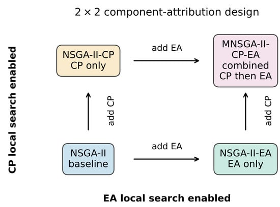
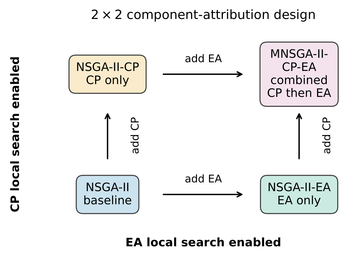
We therefore evaluate two local-search components in a 2 × 2 factorial design using a common NSGA-II backbone. Critical-path (CP) search primarily targets the makespan-oriented region, whereas energy-aware (EA) search primarily targets total energy consumption (TEC). Enabling or disabling each component gives four variants: NSGA-II, NSGA-II-CP, NSGA-II-EA, and memetic NSGA-II with critical-path and energy-aware local search (MNSGA-II-CP-EA). This four-variant design forms the basis for estimating component effects, constructing empirical quality indicators, comparing benchmarks, and conducting the statistical analysis.

The wider repository also includes the Strength Pareto Evolutionary Algorithm 2 (SPEA2) and Multiobjective Evolutionary Algorithm Based on Decomposition (MOEA/D) as independent external comparators. We exclude these algorithms from the primary empirical reference set, factorial effects, rankings, statistical inference, and conclusions. Comparing complete algorithms addresses a different question from isolating component effects within a common backbone. Archived SPEA2 fronts are used only in the separately identified post hoc sensitivity analysis of the empirical reference set.

The study is organised around four research questions:

• RQ1: Does enabling CP improve the makespan-oriented region consistently, both when EA is absent and when it is present?
• RQ2: Does enabling EA improve the energy-oriented region consistently, both without CP and in the presence of CP?
• RQ3: How do CP and EA influence the quality of the final Pareto-front approximation, and how are their joint effects classified under the author-defined criteria for additivity, synergy, or antagonism?
• RQ4: What additional wall-clock cost is associated with these component effects under the common generation budget used in the completed experiment?

Here, wall-clock cost means elapsed time around one complete in-memory algorithm invocation; it is distinct from the number of deterministic schedule decodes and is defined precisely in Section 2.3.5.

The purpose of the study is therefore not simply to identify the highest-ranking algorithm. Its contributions are the following:

• A paired 2 × 2 design that estimates the marginal and interaction effects of two objective-specialised local searches while holding representation, decoder, backbone parameters, seed, and initial population constant.
• Implementation-faithful definitions, pseudocode, deterministic examples, telemetry, and benchmark-level statistics that separate objective extremes, final-front indicators, interaction classification, and computational effort.
• Deterministic sensitivity analyses for the empirical reference context, interaction threshold, and idle-energy accounting convention, while distinguishing post hoc calculations from new optimisation experiments.

An equal decoder-evaluation comparison is outside this experiment’s scope and requires a separate controlled study.

The remainder of the paper reviews relevant energy-aware and memetic scheduling research, defines the scope of the derived benchmarks and both local-search procedures, describes the paired experiment and statistical procedures, reports component and sensitivity results, and closes with practical implications, limitations, and three main conclusions.

Table 1 and Figure 1 summarise the four-variant component design.

Table 1. Four-variant factorial design for estimating the effects of critical-path (CP) and energy-aware (EA) local search.

Variant	CP	EA	Treatment	Interpretive Role
NSGA-II	Off	Off	Common backbone	Common evolutionary backbone
NSGA-II-CP	On	Off	CP only	CP-only makespan intensification
NSGA-II-EA	Off	On	EA only	EA-only energy intensification
MNSGA-II-CP-EA	On	On	CP then EA	Combined CP-then-EA treatment

Notes: CP = critical-path local search; EA = energy-aware local search. In the combined variant, CP precedes EA.

Figure 1. The 2 × 2 critical-path (CP)–energy-aware (EA) component design within the Nondominated Sorting Genetic Algorithm II (NSGA-II) backbone. Arrows show component addition; CP precedes EA in the combined variant.

1.1. Related Work

1.1.1. Energy-Aware Flexible Job Shop Scheduling

Research on the FJSP includes exact approaches, dispatching methods, neighbourhood search, metaheuristics, and hybrid algorithms. Recent reviews illustrate both the maturity of the field and the considerable variation in the assumptions used across studies [2]. A similar diversity is found in energy-efficient production scheduling.

Energy-aware scheduling models differ considerably in what they include. Depending on the application, energy consumption may account for processing and idle power, machine start-up and shutdown states, setup and transport activities, variable operating speeds, electricity tariffs, or carbon intensity [3]. These modelling choices are important because they affect not only the calculated objective values but also the scheduling decisions that an algorithm is encouraged to make.

For the FJSP specifically, mixed-integer formulations have considered processing and idle energy jointly with makespan [5], while other green scheduling approaches have combined machine-assignment decisions with explicit energy-saving measures [6]. Gong et al. [4] extended this line of research through the energy-efficient FJSP with discrete operation-sequence flexibility (FJSPDS), where the ordering of operations within a job may itself be flexible.

Several MDPI studies show how practical constraints and energy-saving decisions shape the scheduling model. Zhang et al. [19] combined machine switching with scheduling to minimise makespan and total energy consumption. Their model accounts for transportation, and their NSGA-II searches machine assignments and operation sequences. Meng et al. [20] formulated an MILP with sequence-dependent setups and transportation. Its energy objective includes processing, setup, idle, transportation, and common energy. Liu et al. [21] considered overlapping consecutive operations and transportation times in an energy-minimising model solved by a discrete interior search algorithm. These extensions affect both schedule feasibility and the energy assigned to a schedule.

These search methods also differ in their objectives and local-search mechanisms. Li et al. [22] proposed modified migrating birds optimisation for total energy minimisation, with five neighbourhood structures, local search, and ageing-based reinitialisation. Luan et al. [23] developed discrete whale optimisation with crossover-based updates and variable neighbourhood search. Their low-carbon FJSP objective combines completion-time and energy-consumption costs. Their later improved sparrow search algorithm [24] addressed energy-saving scheduling with power-consumption and processing costs, using adaptive search mechanisms and variable neighbourhood search. These combined cost objectives differ from the separate makespan and energy objectives used here.

In multi-objective memetic search, Wang et al. [25] combined a cellular population structure with variable neighbourhood search to minimise makespan and total energy consumption in an FJSP with controllable processing times. This study illustrates how global and local search can be combined. It also includes a decision variable—processing time—that is fixed in the present experiments.

Recent studies combine more detailed energy models with several search mechanisms. Wang and Zhao [26] combined machine-restart decisions, two neighbourhood searches, and adaptive operator selection in a bi-objective low-carbon FJSP memetic algorithm. Li et al. [27] used Q-learning to select low-level heuristics and critical-path-based speed adjustments for a distributed variable-speed FJSP with makespan and TEC objectives. These integrated algorithms address broader problem variants. The present study instead estimates the marginal and interaction effects of two objective-specialised local-search components within a common backbone.

Recent MDPI studies also illustrate the range of hybrid methods. Shi et al. combined reinforcement learning with a multi-objective evolutionary algorithm for energy-efficient FJSP scheduling [28]. Wen et al. proposed an improved NSGA-II for green FJSP scheduling [29], and Liu et al. developed a domain-knowledge-driven memetic method with machine on–off decisions for the distributed FJSP [30]. The review by Fernandes et al. [31] organises energy-efficient job shop research by shop-floor type, energy-efficiency strategy, objectives, problem features, and solution approaches. This framework helps explain the differences among these studies. Together, the studies motivate hybrid search and an explicit definition of the energy convention. The component effects reported here remain conditional on the tested fixed-sequence instances, common generation budget, and CP-then-EA ordering. They do not establish performance under the other formulations reviewed above.

The experiments therefore use fixed-sequence energy-aware FJSP instances derived from FJSPDS sources, rather than the original sequence-flexible decision space.

1.1.2. Critical-Path Neighbourhoods and Memetic Intensification

Routing and sequencing neighbourhoods have played an important role in FJSP metaheuristics for many years [1]. In classical job shop scheduling, critical-block neighbourhoods focus the search on operations that determine the current makespan, thereby avoiding the need to explore a much larger unrestricted neighbourhood [12]. Related work on the FJSP extended this idea to neighbourhoods in which both operation sequencing and eligible-machine assignment can be changed [11]. Such schedule-aware mechanisms have subsequently been incorporated into hybrid genetic algorithms, bottleneck-shifting procedures, and tabu-search approaches [9,10].

Recent work also targets the efficiency and depth of neighbourhood exploration. García Gómez et al. [32] proposed lower and upper bounds for FJSP move evaluation, while Zhang et al. [33] embedded adaptive decomposed-MILP local search in a co-evolutionary job shop matheuristic. These studies pursue efficient composite solvers; the present experiment instead quantifies which local-search component changes which Pareto-front region and at what measured computational cost.

The CP operator considered in this study follows this general line of research, but it is not intended as a reproduction of a particular published algorithm. Starting from the decoded schedule, it extracts one deterministic source-to-terminal critical path and its critical blocks. The resulting neighbourhood includes deduplicated adjacent swaps, boundary insertions, and eligible-machine reassignments for critical operations. A candidate is accepted if it reduces makespan by more than the numerical tolerance $\epsilon$. When the candidate makespan differs from the current makespan by no more than $\epsilon$, the move must instead reduce TEC by more than $\epsilon$. This acceptance rule is part of the specific implementation evaluated here and is therefore relevant to the interpretation of the experimental results.

1.1.3. Energy-Aware Machine Reassignment

Machine assignment directly affects both processing time and processing-energy consumption in energy-aware FJSP models [4,5,6]. Changing the machine assigned to a single operation can therefore reduce its direct energy requirement, but it may simultaneously alter machine utilisation, idle time, and the overall makespan. The EA operator used here exhaustively considers one-gene eligible-machine alternatives for every operation and selects the best admissible improvement. A candidate is admissible only if it reduces TEC by more than $\epsilon$ while increasing makespan by no more than $\epsilon$. Among admissible candidates, the operator first retains the minimum-TEC tolerance band, then the minimum-makespan tolerance band, and finally resolves remaining ties deterministically by global operation index and machine index.

Published energy-aware scheduling studies motivate the use of machine-assignment search [13,14]. However, the precise rule used here—reducing TEC while limiting the makespan increase to the numerical tolerance—is specific to this implementation. We therefore do not attribute this rule to a previous study or present it as a standard named neighbourhood. The factorial experiment directly estimates the effect of adding this operator.

1.1.4. Multi-Objective Memetic Algorithms and Component Attribution

Memetic evolutionary algorithms combine population-level exploration with individual learning or local improvement [8]. In multi-objective optimisation, local search can affect proximity to an empirical reference set, the distribution of solutions along the approximate front, and the objective extremes. NSGA-II provides the common backbone in this study [7]. Hypervolume (HV) measures the dominated objective-space volume relative to a fixed reference point. Inverted generational distance (IGD) measures distance from a reference approximation to the evaluated approximation, whereas Deb-style Spread measures distribution regularity [7,34,35]. These indicators describe different aspects of solution quality and should be interpreted separately.

Computational experiment design also matters: paired instances and seeds reduce nuisance variation, while multiple-problem inference should treat benchmark instances, rather than individual runs, as the independent experimental blocks [15,16,18]. Controlled ablation helps attribute observed performance differences to specific configuration components [17]. Accordingly, the present analysis uses benchmark-level effects and exact rank procedures. A statistically and practically explicit interaction rule further distinguishes “the combination ranks first” from “the components are synergistic”.

Scheduling-specific evidence reinforces the value of component-level analysis: Rolim and Nagano [36] reimplemented 12 metaheuristics under standardised conditions and analysed how representation, neighbourhood, and acceleration choices affected performance. The present work applies that attribution logic to a paired 2 × 2 bi-objective energy-aware FJSP design rather than comparing complete algorithms.

2. Materials and Methods

2.1. Problem Definition and Benchmark Boundary

2.1.1. Fixed-Sequence Bi-Objective FJSP

Let $\mathcal{J}$ be the set of jobs, ${\mathcal{O}}_j=(1,\dots ,n_j)$ the fixed operation sequence of job j, and $\mathcal{M}$ the machine set. Operation $(j,o)$ is eligible on $m\in {\mathcal{M}}_{jo}$, with processing duration $p_{jom}>0$. Binary $x_{jom}$ equals one when that alternative is selected; $S_{jo}$ and $C_{jo}$ are its start and completion times. Feasibility requires

$$\sum _{m\in {\mathcal{M}}_{jo}}{x}_{jom}=1,x_{jom}\in \{0,1\},S_{jo}\ge 0,$$

(1)

$$C_{jo}=S_{jo}+\sum _{m\in {\mathcal{M}}_{jo}}{p}_{jom}{x}_{jom},S_{j,o+1}\ge C_{jo},$$

(2)

for every applicable job and operation. For any two distinct operations a and b assigned to the same machine, capacity additionally requires the disjunction $C_a\le S_b$ or $C_b\le S_a$. The implementation enforces this relation through deterministic schedule generation rather than a big-M formulation. The first objective is

$$C_{\max }=\underset{j\in \mathcal{J},o\in {\mathcal{O}}_j}{\max }{C}_{jo}.$$

(3)

Let $P_m^{\mathrm{proc}}$ and $P_m^{\mathrm{idle}}$ be the proportional processing- and idle-power coefficients. Define machine load and the active-machine set as

$$L_m=\sum _{j\in \mathcal{J}}\sum _{o\in {\mathcal{O}}_j:m\in {\mathcal{M}}_{jo}}{p}_{jom}{x}_{jom},{\mathcal{M}}_{\mathrm{act}}=\{m\in \mathcal{M}:L_m>0\}.$$

(4)

The second objective has processing-energy ($PE$) and common-horizon idle-energy ($I{E}^{\mathrm{CH}}$) components:

$$PE=\sum _{j\in \mathcal{J}}\sum _{o\in {\mathcal{O}}_j}\sum _{m\in {\mathcal{M}}_{jo}}{P}_m^{\mathrm{proc}}{p}_{jom}{x}_{jom},$$

(5)

$$I{E}^{\mathrm{CH}}=\sum _{m\in {\mathcal{M}}_{\mathrm{act}}}{P}_m^{\mathrm{idle}}(C_{\max }-L_m),$$

(6)

$$TE{C}^{\mathrm{CH}}=PE+I{E}^{\mathrm{CH}}.$$

(7)

The resulting bi-objective optimisation problem is formally defined as follows:

$$\underset{x,S,C}{\min }\left(C_{\max },TE{C}^{\mathrm{CH}}\right).$$

(8)

The common horizon is $[0,C_{\max }]$. Each active machine is assumed to remain available in standby throughout this interval, so $C_{\max }-L_m$ includes idle time before its first operation, between operations, and after its last operation. Unused machines are treated as off. The power coefficients and resulting $TEC$ values are expressed in proportional units rather than calibrated watts or watt-hours. The model excludes setup, transport, start-up and shutdown, sleep states, variable speed, tariffs, and carbon intensity. Section 2.3.6 also examines an operating-window convention that counts only idle gaps between each active machine’s first start and last completion.

2.1.2. Representation and Deterministic Decoding

Each candidate has an operation-sequence (OS) chromosome and a machine-assignment (MA) chromosome. OS contains a multiset of job identifiers: the kth occurrence of job j denotes its kth operation in the fixed sequence. MA is indexed by global operation ID and stores one eligible zero-based machine ID for each operation.

The decoder scans OS from left to right. For each operation, it determines the release time from the immediate job predecessor and inserts the operation into the earliest gap on its assigned machine that can accommodate the full processing duration. Machine intervals are ordered by start time, completion time, and operation ID. Boundary contact is permitted within $\epsilon ={10}^{-9}$. Every local-search candidate is fully decoded and checked for machine eligibility, job precedence, machine non-overlap, and exactly one occurrence of every operation. Objective changes are not estimated incrementally.

The same representation and decoding procedure are used for all four algorithmic variants. This is important for the ablation design because differences between treatments can then be attributed to the local-search components rather than to changes in how schedules are represented or constructed.

2.1.3. Benchmark Provenance and Semantic Limitation

The experimental set comprises 14 instances: PSF01–PSF10, PSF18–PSF19, and PSF23–PSF24. Their sizes range from 10 to 20 jobs, 7 to 10 machines, and 50 to 100 operations.

The retained annotated FJSPDS files identify, for every job, a constrained-operation count $c_j$ and, where applicable, a sequence-free count $f_j=n_j-c_j$. The reproducible projection reads exactly $c_j$ constrained records followed by $f_j$ free records, removes only those class-count fields and grouping parentheses, and writes all operation records in their original textual order. The two power-parameter rows are moved unchanged to the energy registry. Token-level validation across all 14 files reproduced the normalised instances and preserved each machine alternative and processing time. In total, the sources contain 682 constrained and 343 sequence-free operations.

The conversion treats the recorded operation order as one complete fixed precedence chain, with the formerly sequence-free operations following the constrained operations. It therefore preserves one linear ordering, but not the original FJSPDS sequencing decision space. The results apply to the derived fixed-sequence energy-aware FJSP instances and must not be interpreted as direct FJSPDS performance [4]. Table 2 summarises the instance dimensions. The revision artefacts include a deterministic validator, a per-file table of source and derived SHA-256 hashes, and the conversion specification. Third-party redistribution rights must be confirmed independently before the annotated sources are released publicly.

Table 2. Benchmark dimensions.

Instance	Jobs	Machines	Operations
PSF01	10	7	50
PSF02	10	7	50
PSF03	10	7	50
PSF04	10	7	50
PSF05	10	7	50
PSF06	15	7	75
PSF07	15	7	75
PSF08	15	7	75
PSF09	15	7	75
PSF10	15	7	75
PSF18	20	10	100
PSF19	20	10	100
PSF23	10	10	100
PSF24	10	10	100

2.2. Component-Based Search Framework

2.2.1. Common NSGA-II Backbone

All four treatments use the same implementation of NSGA-II [7]. The population size is 120, the algorithm runs for 100 generations, the crossover probability is 0.70, and the mutation probability is 0.15. Binary tournaments select parents using nondomination rank and crowding distance, followed by elitist environmental replacement.

Offspring are generated using complementary job-subset operation-based crossover (OBX) for OS and uniform crossover with a shared Boolean mask for MA. Independent mutation decisions apply OS swaps between positions containing different job IDs and MA reassignment of one mutable operation to a uniformly sampled alternative eligible machine. The initial population uses random eligible-machine assignments for 50% of individuals, shortest-processing-time assignments for 25%, and lowest-processing-energy assignments for 25%; OS chromosomes are shuffled. For each benchmark–seed pair, the serialised initial population and its signature are identical across all four treatments.

All variants also use the same generation budget. The backbone evaluates 120 initial individuals and 120 offspring in each of 100 generations, giving 12,120 population evaluations before accounting for local search. Each recorded CP or EA candidate evaluation adds one complete decoder call, so the exact total for a run is $\mathrm{12,120}+n_{\mathrm{CP}}+n_{\mathrm{EA}}$. Because intermediate populations and checkpoints were not archived, we cannot reconstruct solution quality at a common decoder-evaluation or time limit.

2.2.2. Critical-Path Local Search

CP is active in NSGA-II-CP and MNSGA-II-CP-EA. In every generation, nondomination rank and crowding distance are assigned to the 120 offspring. The offspring are ordered by ascending nondomination rank, descending crowding distance within rank, and ascending individual ID as the final tie-breaker; the first $\lceil 0.35\times 120\rceil =42$ individuals are selected for local search. A CP call constructs the decoded schedule’s critical structure and generates a deduplicated neighbourhood containing adjacent swaps within critical blocks, first/last boundary insertions, and eligible-machine reassignments for critical operations. Precedence-invalid sequence moves are skipped.

CP candidates are examined in a fixed deterministic order using a first-improvement strategy. A candidate is accepted when it reduces makespan by more than $\epsilon$. If its makespan differs from the current makespan by no more than $\epsilon$, the candidate must instead reduce TEC by more than $\epsilon$. Each CP call in the reported experiment accepts no more than one move. The implementation recomputes the critical structure between accepted moves when a configuration permits multiple moves, but that iterative case is not used here. CP is therefore primarily a makespan-oriented operator, with TEC used only to distinguish solutions whose makespans are equal within the numerical tolerance.

Implementation-Faithful CP Pseudocode

Given an evaluated individual u and accepted-move cap K (here $K=1$):

1.

Select the smallest global operation ID completing within $\epsilon$ of $C_{\max }\left(u\right)$. Trace backwards by taking a tight immediate machine predecessor when present and otherwise a tight immediate job predecessor. Reverse the trace and identify maximal same-machine segments of at least two operations as critical blocks.

2.

Build one ordered neighbourhood. For each block in path order, add adjacent exact-operation swaps, moves of the first block operation after each later operation (nearest first), and moves of the last operation before each earlier operation (nearest first). Then, add every alternative eligible-machine assignment for each critical-path operation in global-operation and machine-ID order.

3.

Discard sequence moves that reverse within-job precedence. Verify the exact-operation-order–OS round trip and deduplicate candidates by their complete $(\mathrm{OS},\mathrm{MA})$ tuple, retaining the first occurrence.

4.

Fully decode candidates in that order. Accept the first v satisfying

$$C_{\max }\left(v\right)<C_{\max }\left(u\right)-\epsilon \mathrm{or}\left(|C_{\max }\left(v\right)-C_{\max }\left(u\right)|\le \epsilon \wedge TEC\left(v\right)<TEC\left(u\right)-\epsilon \right).$$

(9)

Stop after the first accepted move or after exhausting the neighbourhood; if $K>1$, recompute the path and neighbourhood from the accepted solution.

The candidate counter excludes the starting solution and includes only trial chromosomes decoded before acceptance or exhaustion.

Illustrative CP Calculation

This deterministic test fixture is explanatory, not a transition recovered from the historical runs. For four two-operation jobs and three machines, let the eight processing-time vectors be $(8,2,1)$, $(8,7,7)$, $(5,7,7)$, $(3,3,8)$, $(3,8,1)$, $(1,4,8)$, $(8,3,9)$, and $(2,1,5)$; let $P^{\mathrm{proc}}=(5,4,6)$, $P^{\mathrm{idle}}=(1,0.8,1.2)$, $\mathrm{OS}=(0,0,2,2,3,1,3,1)$, and $\mathrm{MA}=(0,2,0,1,2,1,2,0)$. Decoding gives $(C_{\max },PE,I{E}^{\mathrm{CH}},TE{C}^{\mathrm{CH}})=(26,205,37,242)$. The selected path is $(0,1,6,7)$ and block $(1,6)$ lies on machine 2 (zero-based). Swapping those two exact operations is the first candidate and gives $(17,205,10,215)$, so it is accepted after one decoded candidate.

2.2.3. Energy-Aware Local Search

EA is enabled in NSGA-II-EA and MNSGA-II-CP-EA. Like CP, it is applied to the deterministic 35% subset of offspring selected for local improvement. EA uses exhaustive best improvement rather than the first-improvement strategy used by CP.

For each operation, EA examines every other eligible machine except the operation’s current assignment. A candidate therefore differs from the current individual in exactly one MA gene, after which the complete schedule is decoded again. To be admissible, the reassignment must reduce TEC by more than $\epsilon$ and may increase makespan by no more than $\epsilon$.

Rather than accepting the first admissible change, EA evaluates the available alternatives and selects the best one. It first retains candidates within $\epsilon$ of the minimum admissible TEC, then those within $\epsilon$ of the minimum makespan in that energy band, and finally resolves remaining ties by global operation index and machine index. Only one reassignment can be accepted during a single EA call.

This exhaustive one-gene scan gives EA a substantially broader search scope than the structurally restricted CP neighbourhood. It also explains why the number of EA candidates can be much larger than both the number of ordinary population evaluations and the number of CP candidates. Thus, EA was not matched to the other treatments by candidate evaluations.

Implementation-Faithful EA Pseudocode

Given evaluated u and cap K (here $K=1$):

1.

For each operation in ascending global ID and each alternative eligible machine in ascending ID, preserve OS, change only that MA gene, fully decode the candidate v, and increment the candidate counter.

2.

Retain v only if $TEC\left(v\right)<TEC\left(u\right)-\epsilon$ and $C_{\max }\left(v\right)\le C_{\max }\left(u\right)+\epsilon$.

3.

If none is admissible, stop. Otherwise, find the global minimum TEC, retain its $\epsilon$ band, find the minimum makespan inside that band, retain its $\epsilon$ band, and choose the lexicographically smallest (operation ID, target machine ID) among remaining ties.

4.

Accept that candidate; if $K>1$, enumerate the complete one-gene neighbourhood again from the new solution.

The makespan restriction prevents EA from undoing a material CP gain, but it also excludes potentially nondominated lower-energy schedules with larger makespan. EA therefore searches among solutions with nearly unchanged makespan, rather than across the unrestricted bi-objective neighbourhood. This restriction may limit the extent and diversity of the resulting front.

Illustrative EA Calculation

Consider one operation that is eligible on four machines, has duration 4 on each, and has processing-power coefficients $(5,4,3,2)$. The current zero-based machine-0 assignment gives $(C_{\max },TEC)=(4,20)$. Reassignments to machines 1, 2, and 3 give $(4,16)$, $(4,12)$, and $(4,8)$. EA decodes all three admissible candidates and selects machine 3, demonstrating exhaustive best improvement. In a separate tolerance example, changing $(C_{\max },TEC)=(1,10)$ to $(4,6)$ is rejected despite its energy saving because the makespan increase is larger than $\epsilon$.

2.2.4. CP-Then-EA Integration and Factorial Design

When both local-search components are active, CP is applied first and EA immediately afterwards to the same selected offspring. This ordering is part of the combined treatment itself. The estimated interaction consequently refers specifically to a CP-then-EA configuration; it should not be generalised to EA-then-CP or repeated alternating search without additional experiments.

As summarised in Table 1 and Figure 1, the 2 × 2 design defines four planned component contrasts. We evaluate the effect of adding CP both without EA and with EA present in the configuration. Similarly, we evaluate the effect of adding EA both without CP and with CP present. The corresponding comparisons are NSGA-II versus NSGA-II-CP, NSGA-II-EA versus MNSGA-II-CP-EA, NSGA-II versus NSGA-II-EA, and NSGA-II-CP versus MNSGA-II-CP-EA, respectively. These contrasts describe component presence, not changes in execution order: the combined variant always applies CP before EA. No EA-then-CP treatment was archived, so this design cannot estimate operator-order effects. Those effects require a future experiment.

2.3. Experimental Design and Statistical Analysis

2.3.1. Paired Experimental Design and Output Validation

The experiment conducted for this study comprised 14 benchmarks × 10 seeds × 4 variants = 560 complete and unique runs. Automated checks confirmed finite required values, intact initial-population pairing, agreement between primary and release artefacts, and consistency between recorded chromosomes and final-front objective vectors. Full SHA-256 and signature results are reported in the evidence audit available in the repository listed in the Data Availability Statement. Supporting scripts, analysis outputs and provenance records are provided in the Supplementary Materials.

For each benchmark, we pooled all objective vectors from the 40 final rank-zero fronts produced by NSGA-II, NSGA-II-CP, NSGA-II-EA, and MNSGA-II-CP-EA over seeds 1001–1010. We removed exact duplicate vectors and retained the nondominated vectors under minimisation (≤ in both objectives and < in at least one). This set provides the empirical IGD reference; it is an experimental approximation, not a known global Pareto front.

We used the componentwise minimum ${\ell }_j$ and maximum $u_j$ of this reference set to normalise all fronts and the reference set as $(f_j-{\ell }_j)/s_j$, where $s_j=u_j-{\ell }_j$ or 1 when the span is zero. The common normalised HV reference point was $r_j={\max }_{x\in P}(x_j-{\ell }_j)/s_j+0.1$, where P is the entire 40-front pool before duplicate removal and nondominance filtering. We used the same benchmark-specific normalisation and reference point for all 40 runs.

To assess sensitivity to the empirical reference, we added the ten archived SPEA2 final fronts to each benchmark’s pool and rebuilt the reference set. We then re-evaluated the four target variants under the primary and SPEA2-augmented reference settings. This post hoc analysis changes only the normalisation and empirical reference approximation. It adds no optimisation runs, and SPEA2 remains outside the factorial inference.

Minimum makespan and minimum TEC were extracted independently from each final nondominated front. The two extrema may belong to different schedules. HV is higher-is-better, whereas IGD and Spread are lower-is-better. Spread follows the NSGA-II distribution measure [7].

2.3.2. Primary Paired Component Contrasts

For each planned contrast and benchmark, we first calculated ten paired differences, one for each shared seed. We oriented these differences so that positive values always favour adding the component: component-added minus component-absent for metrics where higher values are better, and component-absent minus component-added for metrics where lower values are better. The effect for each benchmark is the median of its ten paired differences. Statistical inference therefore uses 14 benchmark effects, rather than treating the 140 seed records as independent problems.

We tested the 14 benchmark effects using an exact two-sided Wilcoxon signed-rank procedure [37]. We discarded exact zeros, assigned average ranks to tied absolute values, and enumerated all sign assignments. Rank-biserial correlation is oriented so that positive values favour the variant with the component added [38]. Holm’s sequential correction was applied to the four planned contrasts separately for each metric [39].

We calculated descriptive 95% percentile-bootstrap intervals over the 14 benchmark blocks using 10,000 resamples and seed 20260828 [40]. Interaction intervals use the same resampling design and seed. With only 14 blocks, these intervals describe variation across benchmarks and should not be interpreted as precise population bounds.

2.3.3. Factorial Effects and Interaction Classification

Within each benchmark and seed, let $Y_{00}$, $Y_{10}$, $Y_{01}$, and $Y_{11}$ denote the outcome for the baseline, CP-only, EA-only, and combined treatments. The raw factorial interaction is

$$I=Y_{11}-Y_{10}-Y_{01}+Y_{00}.$$

(10)

For outcomes where lower values are better, we reversed the sign so that positive effects indicate improvement. For each benchmark, medians across seeds were expressed as percentages of $Y_{00}$. CP, EA, and interaction effects formed one three-effect Holm correction family for each metric. We calculated cross-benchmark p-values using exact sign-flip inference.

To interpret interaction, we applied an author-defined symmetric 2% threshold to the descriptive 95% bootstrap interval. An interaction is classified as synergistic if the entire interval is above +2%, antagonistic if it is below −2%, approximately additive if it is within [−2%, +2%], and uncertain otherwise. The two-percentage-point margin treats changes within this band as practically negligible relative to baseline. It is an author-defined judgement, not a significance threshold or an established field standard. Statistical evidence of a nonzero interaction alone is therefore insufficient to classify it as practically synergistic or antagonistic.

The sensitivity of these labels follows algebraically from the stored intervals and requires no experiment rerun. We report classifications on the prespecified grid $T\in \{0,1,2,3,5\}\%$. For any interval $[L,U]$, the label is synergistic if $L>T$, antagonistic if $U<-T$, approximately additive if $L\ge -T$ and $U\le T$, and uncertain otherwise.

2.3.4. Omnibus Comparison and Gated Post Hoc Layer

For HV, IGD and Spread, we calculated each variant’s median across ten seeds to obtain one value per benchmark. The 14 complete benchmark blocks were then analysed using Friedman’s rank test [41]. Kendall’s W summarises rank agreement and effect magnitude [42]. Only when the omnibus test rejected the null hypothesis did we test the four planned post hoc contrasts for that metric, using a separate four-contrast Holm correction family.

This post hoc analysis calculates a seed median for each variant before taking differences between variant medians. The primary analysis instead calculates the median of ten paired seed differences. These operations can produce different effect estimates, signs, and p-values, so the two analyses are reported separately.

2.3.5. Runtime and Cost Boundary

Runtime is wall-clock duration measured around one complete algorithm invocation. For the reported runs, timing begins after the serialised initial population has been loaded from disk and includes its in-memory copying and validation, initial evaluation, all 100 generations, and every enabled local-search call. It excludes serialised-population disk loading, empirical metric-context construction, indicator computation, saving outputs, and plotting. No runtime observation was trimmed, winsorised, or replaced.

The runs were executed on multiple laboratory computers that the authors report had identical nominal hardware configurations. The retained environment records consistently identify a 64-bit Intel Family 6 Model 154 processor with 12 logical processors and Windows build 10.0.26200; they do not preserve the exact computer count, commercial processor name, installed RAM, or Windows edition, so no more specific hardware claim is made. All 14 batch manifests consistently record CPython 3.14.2, NumPy 2.4.0, and SciPy 1.17.0; the analysis environment additionally used pandas 2.3.3, Matplotlib 3.10.8, and PyYAML 6.0.3. Wall-clock comparisons may still contain residual host-load variation even under nominally identical configurations.

Headline runtime ratios pair each benchmark–seed treatment time with its NSGA-II time and then summarise by benchmark. For the descriptive cost-effectiveness table, let $Q_{bv}$ and $t_{bv}$ be the seed-median quality metric and runtime for benchmark b and variant v, and let 0 denote NSGA-II. We compute $q_{bv}=100(Q_{bv}-Q_{b0})/\left|Q_{b0}\right|$ for HV and $q_{bv}=100(Q_{b0}-Q_{bv})/\left|Q_{b0}\right|$ for IGD, $r_{bv}=t_{bv}/t_{b0}$, $\Delta t_{bv}=t_{bv}-t_{b0}$, and $e_{bv}=q_{bv}/(r_{bv}-1)$. Each displayed entry is the median of that quantity over the 14 benchmarks. It is therefore invalid to divide the displayed median quality improvement by the displayed median runtime increment to reconstruct the displayed efficiency. Taking ratios before summarising and taking ratios of benchmark medians can produce different values. We therefore report these runtime summaries separately.

2.3.6. Idle-Energy Sensitivity from Archived Fronts

For an active machine, let $A_m$ and $B_m$ be its first start and last completion. The alternative operating-window convention is

$$I{E}^{\mathrm{OW}}=\sum _{m\in {\mathcal{M}}_{\mathrm{act}}}{P}_m^{\mathrm{idle}}\left[(B_m-A_m)-L_m\right],TE{C}^{\mathrm{OW}}=PE+I{E}^{\mathrm{OW}}.$$

(11)

It charges internal gaps but excludes leading and trailing idle periods. We deterministically decoded all 58,226 chromosomes retained in the 560 final-front archives, first verifying every stored $(C_{\max },TE{C}^{\mathrm{CH}})$ value within ${10}^{-9}$, and then re-scored and refiltered those schedules under $TE{C}^{\mathrm{OW}}$. Because the archive contains original-objective rank-zero fronts rather than complete final populations, this analysis is conditional on retained schedules and is not equivalent to re-optimising under the alternative objective.

3. Results

3.1. RQ1: CP Effects on Objective Extremes

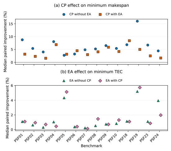
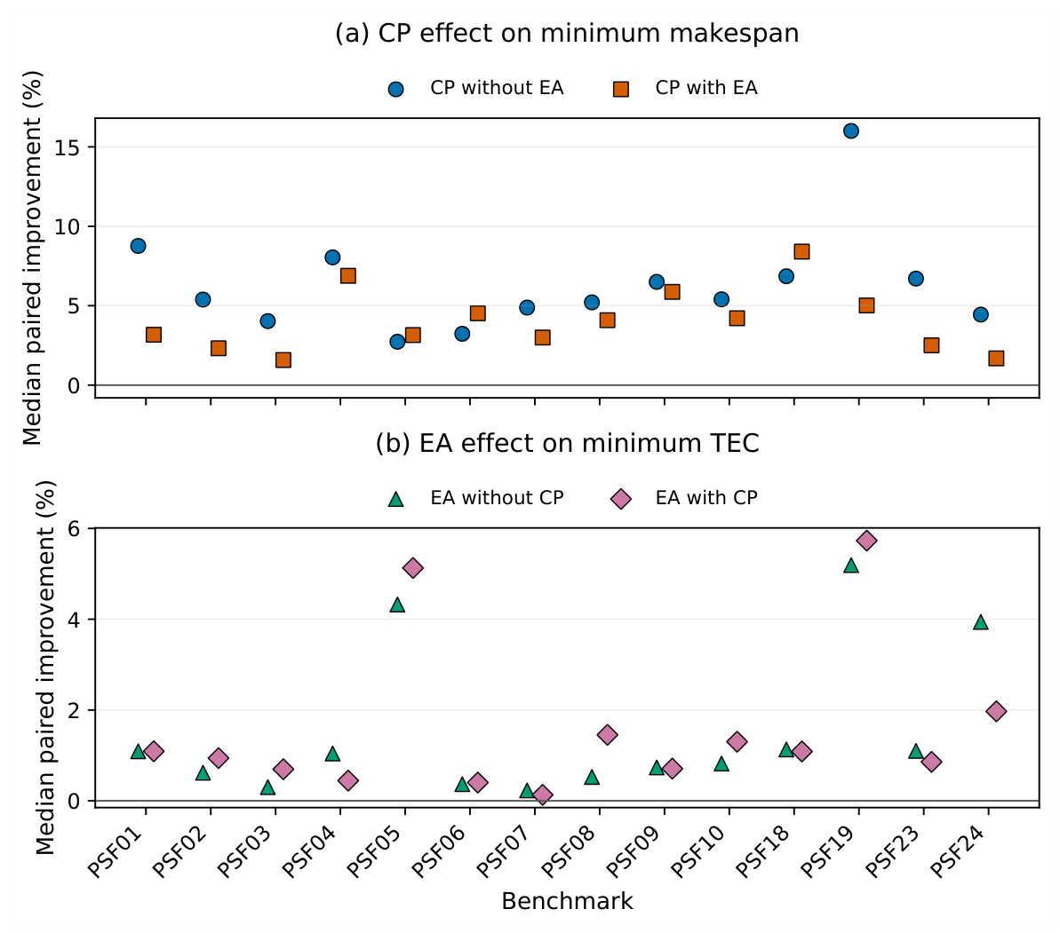
CP produced a large and consistent makespan contribution (Table 3; Figure 2). Without EA, it improved benchmark-level paired minimum makespan by a median 29.75 time units (descriptive 95% bootstrap interval 22.00–39.00), equivalent to 5.4698%. Every benchmark favoured CP; rank-biserial correlation was 1.0000 and the Holm-adjusted exact p-value was 0.000488. With EA already active, CP improved minimum makespan by 19.75 units (11.75–25.00), or 3.6779%. Again, all 14 benchmarks favoured the added component, with rank-biserial 1.0000 and adjusted p = 0.000488.

Table 3. Planned paired component contrasts for minimum makespan.

Contrast	Median Gain [95% Interval]	Median Gain (%)	$+/-/=$	${\mathit{r}}_{\mathbf{rb}}$	Raw p	Holm-Adj. p
CP without EA	29.750 [22.000, 39.000]	5.470	14/0/0	1.0000	0.000122	0.000488
CP with EA	19.750 [11.750, 25.000]	3.678	14/0/0	1.0000	0.000122	0.000488
EA without CP	6.250 [3.000, 21.000]	1.258	13/1/0	0.9143	0.000977	0.001953
EA with CP	−1.750 [−3.500, 2.500]	−0.289	4/9/1	−0.2198	0.508789	0.508789

Notes: Gain is the median of the 14 benchmark-level paired effects, in processing-time units; brackets give descriptive 95% bootstrap intervals. $+/-/=$ counts benchmarks favouring addition, favouring absence, or tied, respectively; $n=14$. Positive effects favour the component-added variant. $r_{\mathrm{rb}}$ is the oriented rank-biserial correlation. Holm’s adjustment covers the four planned contrasts within each outcome. Displayed gains are rounded; calculations use full precision.

Figure 2. Median paired component improvements across benchmarks. Panel (a) shows the CP contrasts for makespan; panel (b) shows the EA contrasts for TEC. Each point is a benchmark median of ten within-seed percentage improvements; positive values favour adding the component.

The cross-objective TEC effects were not comparable in strength. Without EA, adding CP changed minimum TEC by −16.75 proportional units (−159.25–79.00), a median −0.0731%, with a 7–7 benchmark split and adjusted p = 0.714844. With EA, the median TEC improvement was 56.75 units (−6.50–97.50), or 0.1652%; 10 of 14 benchmarks favoured CP, but the contrast did not survive Holm’s correction (adjusted p = 0.156982). These comparisons support a direct role for CP in improving makespan; they do not establish a corresponding reduction in energy.

3.2. RQ2: EA Effects on Objective Extremes

EA produced the corresponding energy-oriented contribution (Table 4; Figure 2). Without CP, it reduced minimum TEC by a median 347.75 proportional units (168.875–640.50), a 0.9367% improvement. All 14 benchmark effects favoured EA; rank-biserial was 1.0000 and adjusted p = 0.000488. With CP enabled, adding EA improved minimum TEC by 428.75 units (178.00–572.50), or 1.0142%; all 14 benchmarks again favoured EA with rank-biserial 1.0000 and adjusted p = 0.000488.

Table 4. Planned paired component contrasts for minimum total energy consumption (TEC).

Contrast	Median Gain [95% Interval]	Median Gain (%)	$+/-/=$	${\mathit{r}}_{\mathbf{rb}}$	Raw p	Holm-Adj. p
CP without EA	−16.750 [−159.250, 79.000]	−0.073	7/7/0	−0.1238	0.714844	0.714844
CP with EA	56.750 [−6.500, 97.500]	0.165	10/4/0	0.5429	0.078491	0.156982
EA without CP	347.750 [168.875, 640.500]	0.937	14/0/0	1.0000	0.000122	0.000488
EA with CP	428.750 [178.000, 572.500]	1.014	14/0/0	1.0000	0.000122	0.000488

Notes: Gain is the median of the 14 benchmark-level paired effects, in proportional energy units; brackets give descriptive 95% bootstrap intervals. $+/-/=$ counts benchmarks favouring addition, favouring absence, or tied, respectively; $n=14$. Positive effects favour the component-added variant. $r_{\mathrm{rb}}$ is the oriented rank-biserial correlation. Holm’s adjustment covers the four planned contrasts within each outcome. Displayed gains are rounded; calculations use full precision.

EA also improved minimum makespan when CP was absent: the median gain was 6.25 time units (3.00–21.00), or 1.2577%, 13 of 14 benchmarks favoured EA, and adjusted p = 0.001953. This secondary makespan benefit was not established when CP was present. Adding EA to NSGA-II-CP yielded a median −1.75-unit oriented effect (−3.50–2.50), or −0.2892%; only four benchmarks favoured EA, nine favoured the CP-only variant, one tied, and adjusted p = 0.508789.

3.3. RQ3: Final-Front Approximation Quality

All three four-variant omnibus tests rejected equal benchmark-level performance (Table 5). For HV, ${\chi }^2\left(3\right)=36.257$, $p=6.607\times {10}^{-8}$, and Kendall’s $W=0.863$. For IGD, ${\chi }^2\left(3\right)=29.914$, $p=1.439\times {10}^{-6}$, and $W=0.712$. For Spread, ${\chi }^2\left(3\right)=22.114$, $p=6.176\times {10}^{-5}$, and $W=0.527$. MNSGA-II-CP-EA had the best average rank for HV (1.000), IGD (1.143), and Spread (1.143); lower average rank is better.

Table 5. Friedman’s omnibus tests and average ranks for final-front approximation quality.

Metric	${\mathit{\chi }}^2\left(3\right)$	p	Kendall’s W	Rank Baseline	Rank CP	Rank EA	Rank CP+EA
HV	36.257	$6.607\times {10}^{-8}$	0.863	3.929	2.643	2.429	1.000
IGD	29.914	$1.439\times {10}^{-6}$	0.712	3.786	2.714	2.357	1.143
Spread	22.114	$6.176\times {10}^{-5}$	0.527	3.286	2.857	2.714	1.143

Notes: Baseline = NSGA-II; CP = NSGA-II-CP; EA = NSGA-II-EA; CP+EA = MNSGA-II-CP-EA. Friedman’s tests use 14 benchmark blocks; lower average rank is better. HV = hypervolume; IGD = inverted generational distance; Spread = Deb-style distribution measure.

The post hoc comparisons performed after the omnibus tests show broad improvements in HV and IGD (Table 6). For HV, every CP and EA contrast survived Holm’s correction, with 13 or 14 of 14 benchmark medians favouring the component-added variant and adjusted p ≤ 0.000488. For IGD, all four contrasts also survived, with 12 or 13 benchmarks favourable and adjusted p between 0.000977 and 0.003418. Spread was more context dependent: CP without EA and EA without CP did not survive correction, whereas CP with EA (14/14 favourable, adjusted p = 0.000488) and EA with CP (12/14 favourable, adjusted p = 0.001831) did.

Table 6. Gated planned post hoc contrasts based on benchmark-level seed medians.

Metric	Contrast	Median Oriented Effect	$+/-/=$	${\mathit{r}}_{\mathbf{rb}}$	Holm-Adj. p
HV	CP without EA	0.7217	13/1/0	0.9810	0.000488
HV	CP with EA	0.7963	14/0/0	1.0000	0.000488
HV	EA without CP	0.7745	14/0/0	1.0000	0.000488
HV	EA with CP	0.6120	14/0/0	1.0000	0.000488
IGD	CP without EA	0.2065	12/2/0	0.8857	0.003418
IGD	CP with EA	0.1589	13/1/0	0.8667	0.003418
IGD	EA without CP	0.3109	13/1/0	0.9810	0.000977
IGD	EA with CP	0.2718	13/1/0	0.9619	0.001099
Spread	CP without EA	0.0333	8/6/0	0.2762	0.390991
Spread	CP with EA	0.0675	14/0/0	1.0000	0.000488
Spread	EA without CP	0.0455	10/4/0	0.5048	0.208008
Spread	EA with CP	0.0793	12/2/0	0.9429	0.001831

Notes: +/−/= counts benchmarks favouring addition, favouring absence, or tied, respectively; n = 14. Positive effects favour the component-added variant. r_rb is the oriented rank-biserial correlation. Holm’s adjustment covers the four planned contrasts within each outcome. Effects are absolute differences in the respective indicator, not percentages. HV is higher-is-better; IGD and Spread are lower-is-better. Tests use benchmark-level seed medians and are gated by the corresponding Friedman test.

The primary analysis of paired differences leads to the same substantive conclusion for HV and IGD. Median HV improvements ranged from 27.01% to 68.03% across the four component contrasts, and median IGD improvements ranged from 23.17% to 33.58%; all eight adjusted p-values were below 0.001. For Spread, only the two contrasts in which the other component was already present remained significant after correction.

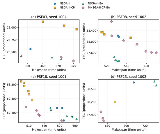
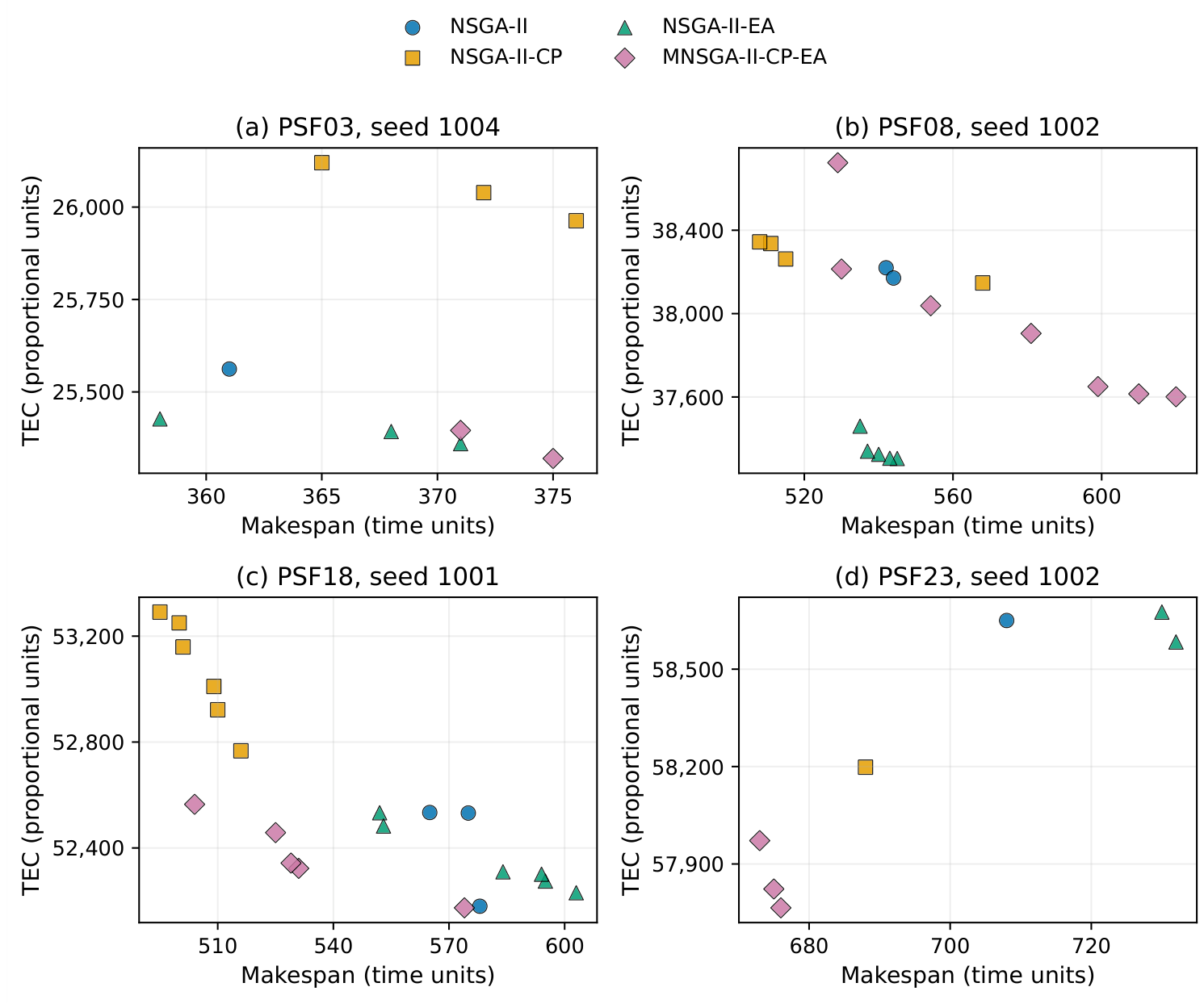
Figure 3 shows representative archived final fronts selected by a fixed rule that does not depend on the combined variant’s performance. Within each observed problem-size stratum, we selected the lower-median benchmark identifier. We then selected the seed whose baseline NSGA-II HV was closest to that benchmark’s baseline median HV, resolving ties by choosing the lower seed. The markers show discrete objective vectors from the final fronts. The figure illustrates their geometry and does not show convergence trajectories.

Figure 3. Archived final-front objective vectors for four benchmark–seed pairs selected by a fixed rule. Distinct marker shapes identify the variants; points are discrete vectors, not trajectories. Both objectives are minimised, so lower-left positions indicate better values. Axis ranges differ between benchmarks; energy is measured in proportional units.

3.4. Empirical-Reference Sensitivity

Adding the ten archived SPEA2 fronts to each benchmark’s empirical context had little effect on the conclusions for the target variants. Across the 56 benchmark–variant medians, Spearman’s correlations between primary and augmented-context values were 0.990 for HV, 0.983 for IGD, and 0.989 for Spread. The best target variant was unchanged for all 14 benchmarks for HV and Spread and for 13 of 14 for IGD. MNSGA-II-CP-EA retained the best average rank for all three metrics (Table 7). This check addresses reference-set dependence while keeping SPEA2 outside the factorial comparison and treating the reference as an empirical approximation.

Table 7. Sensitivity of target-variant results to adding archived SPEA2 fronts to the empirical reference context.

Metric	Spearman’s Correlation	Same Winner (of 14)	Combined Rank Primary	Combined Rank Augmented
HV	0.990	14/14	1.000	1.000
IGD	0.983	13/14	1.143	1.214
Spread	0.989	14/14	1.143	1.143

Notes: Primary: Four target variants only. Augmented: The same targets re-evaluated after adding archived SPEA2 fronts to the empirical reference context. Correlations summarise 56 benchmark–variant medians. Same winner counts agreement across 14 benchmarks; combined denotes CP+EA. Lower rank is better.

3.5. RQ3: Factorial Main Effects and Interaction

Factorial main effects reinforce the specialised-role interpretation. On an oriented scale expressed as a percentage of baseline, the CP main effect on minimum makespan was 4.4137% (95% interval 3.9760–6.1770; adjusted p = 0.000366) whereas its TEC main effect was 0.0545% (−0.2106–0.2102; adjusted p = 1.000). The EA main effect on TEC was 0.9255% (0.5422–1.1955; adjusted p = 0.000366), while its smaller makespan main effect was 0.5924% (0.0473–2.4277; adjusted p = 0.023071). Both components had positive main effects on HV and IGD, and both had smaller positive Spread main effects.

Table 8 applies the author-defined interaction rule. TEC was approximately additive because its interval, −0.2617% to 0.3570%, lay entirely inside ±2%. For makespan, the median interaction was negative (−1.4408%, adjusted sign-flip p = 0.005127). However, its interval (−3.1132% to −1.0865%) crossed the −2% classification threshold, so the interaction was classified as uncertain rather than antagonistic. Consequently, the evidence does not support a general CP × EA synergy claim.

Table 8. Factorial CP × EA interaction assessments under the author-defined threshold.

Outcome	Median Interaction (%) [95% Interval]	$+/-/=$	Raw p	Holm-Adj. p	Classification
Minimum makespan	−1.441 [−3.113, −1.087]	2/12/0	0.002563	0.005127	Uncertain
Minimum TEC	0.101 [−0.262, 0.357]	7/7/0	0.527466	1.000000	Approx. additive
HV	14.661 [−11.398, 23.408]	9/5/0	0.753662	0.753662	Uncertain
IGD	−7.959 [−15.818, 9.600]	5/9/0	0.545410	0.545410	Uncertain
Spread	2.101 [−1.972, 6.631]	9/5/0	0.156250	0.156250	Uncertain

Notes: Intervals are descriptive 95% bootstrap intervals. $+/-/=$ counts positive, negative, or zero benchmark interaction effects; $n=14$. Positive interactions exceed the sum of individual improvements. Classification uses the entire interval and the author-defined $\pm 2\%$ tolerance; Approx. additive = approximately additive. Sign-flip p-values are Holm-adjusted over CP, EA, and interaction effects within each outcome. Display rounding does not change classification.

The threshold grid in Table 9 shows why interaction labels must remain conditional on the author-defined tolerance. Makespan is antagonistic at 0–1%, uncertain at 2–3%, and approximately additive at 5%; minimum TEC changes from uncertain at 0% to approximately additive from 1% onward. The three front-quality interactions remain uncertain across this threshold grid.

Table 9. Interaction-classification sensitivity over symmetric tolerance T.

Outcome	$\mathit{T}=0\%$	$\mathit{T}=1\%$	$\mathit{T}=2\%$	$\mathit{T}=3\%$	$\mathit{T}=5\%$
Minimum makespan	Antagonistic	Antagonistic	Uncertain	Uncertain	Additive
Minimum TEC	Uncertain	Additive	Additive	Additive	Additive
HV	Uncertain	Uncertain	Uncertain	Uncertain	Uncertain
IGD	Uncertain	Uncertain	Uncertain	Uncertain	Uncertain
Spread	Uncertain	Uncertain	Uncertain	Uncertain	Uncertain

Notes: T is the symmetric tolerance on the interaction percentage. Additive means approximately additive: the full descriptive interval lies within $[-T,T]$. Antagonistic means the full interval lies below $-T$; Uncertain means no classification is established. Thresholds are interpretive sensitivity settings, not new experiments.

3.6. RQ4: Runtime and Descriptive Cost-Effectiveness

The quality gains required substantial wall-clock time (Table 10). Median benchmark runtimes were 101.7985 s for NSGA-II, 627.2171 s for NSGA-II-CP, 2393.5920 s for NSGA-II-EA, and 3051.6860 s for MNSGA-II-CP-EA. The corresponding median paired ratios were 1.0000, 5.9716, 23.5630, and 29.8079. Runtime variability increased with local search; raw observations ranged up to 16,071.303 s for CP, 14,522.588 s for EA, and 22,230.273 s for CP+EA.

Table 10. Full-call wall-clock runtime summaries.

Variant	Median Runtime (s) [${\mathit{Q}}_1$, ${\mathit{Q}}_3$]	Paired Runtime Ratio [${\mathit{Q}}_1$, ${\mathit{Q}}_3$]	Raw-Run Range (s)	Runs
Baseline	101.8 [71.4, 134.0]	1.00 [1.00, 1.00]	66.8–290.1	140
CP	627.2 [286.1, 919.3]	5.97 [4.16, 6.57]	193.1–16,071.3	140
EA	2393.6 [1171.7, 5194.2]	23.56 [16.42, 36.73]	910.2–14,522.6	140
CP+EA	3051.7 [1399.8, 6035.9]	29.81 [19.70, 41.94]	1110.6–22,230.3	140

Notes: Baseline = NSGA-II; CP = NSGA-II-CP; EA = NSGA-II-EA; CP+EA = MNSGA-II-CP-EA. $Q_1$ and $Q_3$ denote the first and third quartiles across the 14 benchmark summaries. Ratios are relative to the paired baseline; raw-run ranges include all 140 runs per variant. All runtimes measure the full call in seconds.

Each enabled local search was called 4200 times per run. The median CP candidate count was 108,470.5 for CP-only and 129,557 for the combined variant; the median EA count was 764,400 in both EA-enabled variants. Adding these complete candidate decodes to the 12,120 backbone decodes gives exact historical median totals of 12,120, 120,590, 776,520, and 908,575 for baseline, CP, EA, and combined, respectively. These counts explain why a common 100-generation limit does not imply equal effort, but the absence of intermediate checkpoints prevents a retrospective comparison of solution quality at an equal decoder-evaluation budget.

The aggregate telemetry in Table 11 covers 140 runs for each variant. A no-accept call means that the relevant neighbourhood was exhausted without an accepted move; for CP, first improvement can terminate a successful call before all generated candidates are decoded, whereas EA decodes its complete one-gene neighbourhood. These mechanisms explain the much larger EA candidate total and prevent candidate counts from being treated as an equal computational budget.

Table 11. Archived local-search call and candidate accounting across 140 runs per enabled variant.

Variant	Operator	Calls	Decoded Candidates	Accepted Calls	No-Accept Calls	Accepted per Call
CP	CP	588,000	14,908,992	182,324	405,676	0.3101
EA	EA	588,000	120,876,000	126,148	461,852	0.2145
CP+EA	CP	588,000	17,326,262	134,125	453,875	0.2281
CP+EA	EA	588,000	120,876,000	153,194	434,806	0.2605

Notes: CP = NSGA-II-CP; EA = NSGA-II-EA; CP+EA = MNSGA-II-CP-EA. Counts aggregate 140 runs per variant. Each successful call accepts at most one move. A no-accept call exhausts the relevant neighbourhood without accepting a move; decoded candidates count complete candidate evaluations. Accepted per call is a proportion, not a percentage.

A post hoc diagnostic identified extreme runtimes for descriptive analysis; all observations were retained. Within each variant, it flagged values above $Q_3+1.5\mathrm{IQR}$ and separately used a robust log-runtime z-score threshold of 3.5. Tukey’s rule flagged baseline PSF23/seed 1008 (290.1 s), CP PSF01/seed 1005 (16,071.3 s) and PSF23/seed 1009 (2444.2 s), EA PSF23/seed 1009 (14,522.6 s), and combined PSF23/seed 1009 (22,230.3 s); the robust log-scale check identified the 16,071.3 s CP observation. Every run completed and passed artefact validation. The repeated PSF23/seed 1009 occurrence and high candidate counts are descriptive co-occurrences only: no host-load or per-step trace was archived, so a causal explanation is not available.

Table 12 reports the descriptive cost-effectiveness ratios. Relative to baseline, the benchmark-median analysis found 57.0132%, 60.8138%, and 114.3505% median HV improvements for CP, EA, and CP+EA, respectively. Corresponding IGD improvements were 28.8596%, 37.2071%, and 56.7907%. CP had the greatest median quality percentage per additional runtime multiple in this descriptive calculation: 13.4580 for HV and 4.5359 for IGD. These descriptive ratios do not measure the practical or economic value of the improvements.

Table 12. Descriptive baseline-relative quality and runtime cost-effectiveness.

Metric	Variant	Quality Gain (%)	Runtime Ratio	Extra Time (s)	Gain per Extra Runtime Multiple
HV	CP	57.01	6.25	526.72	13.46
HV	EA	60.81	23.41	2291.34	2.31
HV	CP+EA	114.35	29.85	2949.44	4.48
IGD	CP	28.86	6.25	526.72	4.54
IGD	EA	37.21	23.41	2291.34	1.20
IGD	CP+EA	56.79	29.85	2949.44	1.83

Notes: Baseline = NSGA-II; CP = NSGA-II-CP; EA = NSGA-II-EA; CP+EA = MNSGA-II-CP-EA. Entries are medians across 14 benchmarks. Positive gain denotes increased HV or reduced IGD. Runtime ratios divide benchmark median runtime by baseline median runtime; they differ from paired-seed ratios in Table 10. Gain per extra runtime multiple is the median of benchmark-wise ratios, not a ratio of the displayed medians. These descriptive summaries use a common generation budget; they do not compare equal computational budgets.

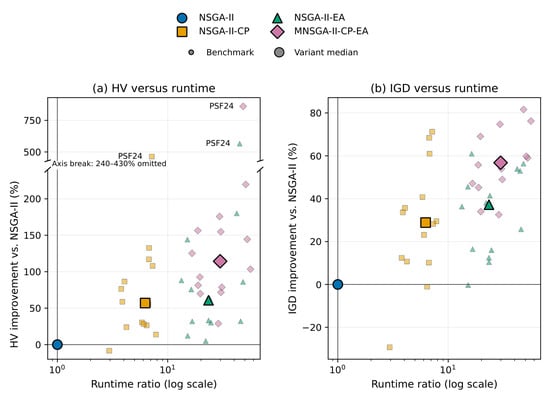
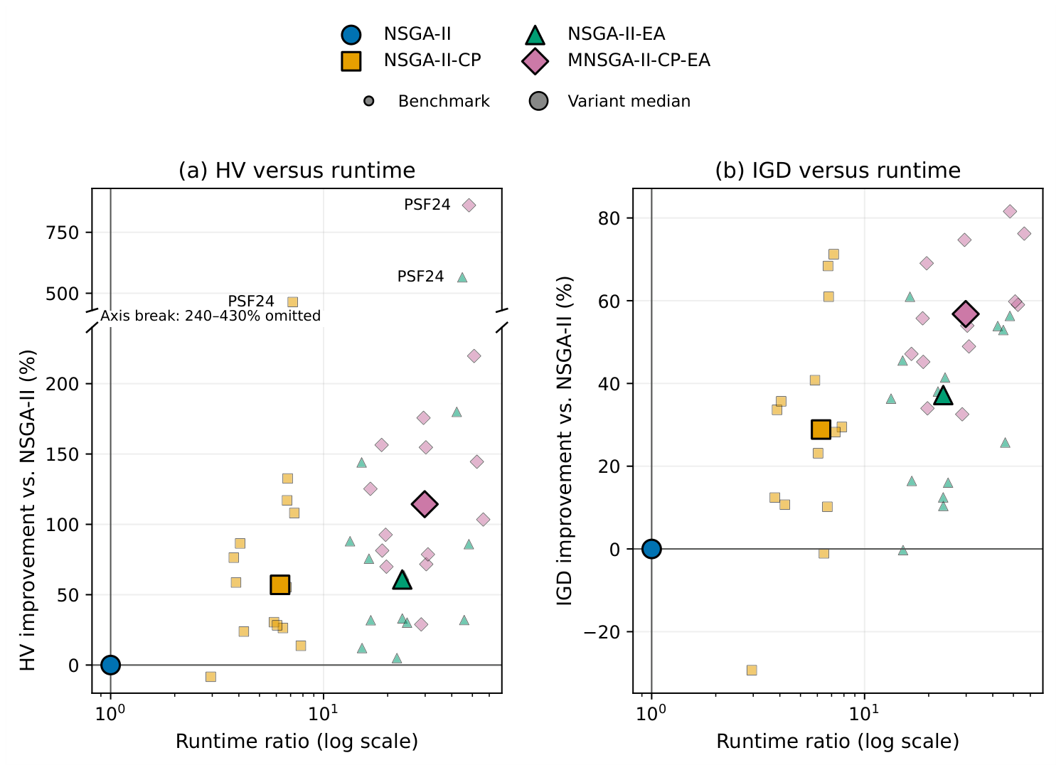
Figure 4 shows the benchmark-level quality/runtime distribution. Its runtime ratios are computed from benchmark medians and therefore differ slightly from the paired-seed headline ratios. The plot documents a common-generation-budget trade-off and is not an equal-decoder-evaluation comparison.

Figure 4. Benchmark-level HV and IGD improvements versus runtime relative to NSGA-II. Smaller markers represent benchmarks and larger outlined markers represent variant medians. The HV axis is broken between 240% and 430% to retain the three high PSF24 observations while preserving detail. The three high HV observations are labelled PSF24. Marker size is explained in the legend. Positive improvement denotes increased HV or reduced IGD; all observations use the existing common generation budget.

A leave-one-benchmark-out influence check cannot substitute for adding instances, but it tests whether one benchmark determines the baseline-relative quality summaries. Across all 14 omissions, median HV improvements remained positive for CP (55.34–58.68%), EA (57.95–63.68%), and CP+EA (103.44–125.26%); the corresponding IGD ranges were 28.24–29.48%, 36.35–38.07%, and 55.75–57.83%. Broader instance families and additional independent runs remain necessary for stronger external validation.

3.7. Schedule Reconstruction and Idle-Energy Sensitivity

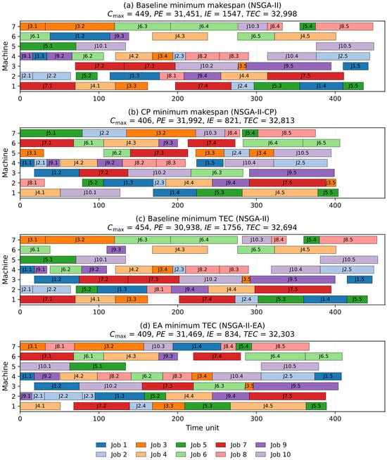
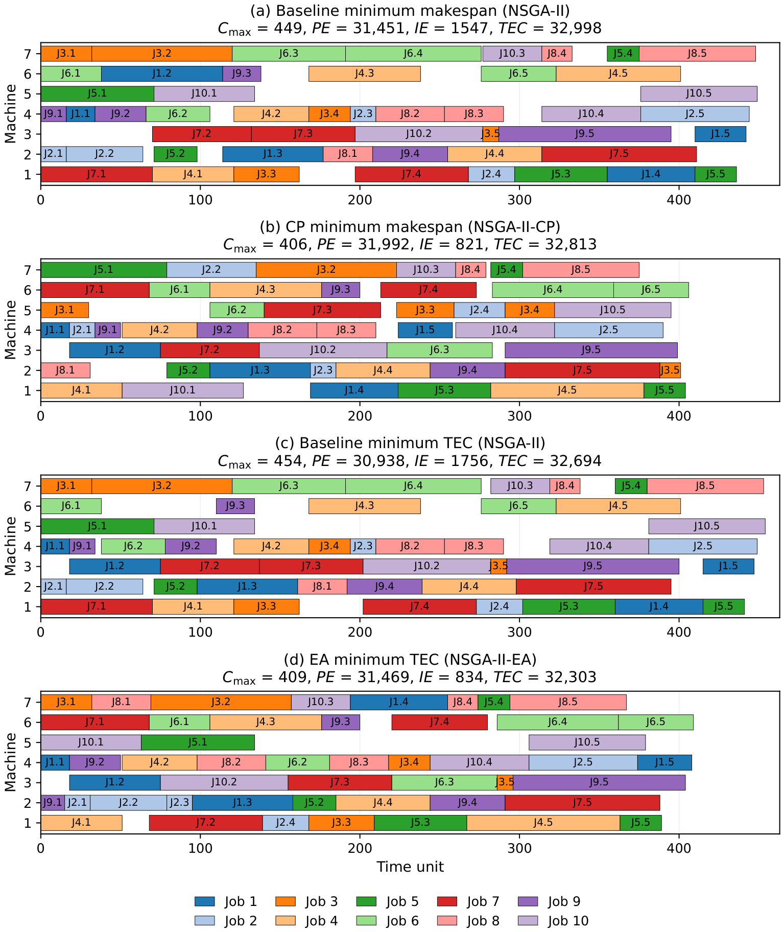
Figure 5 shows four schedules reconstructed from archived final fronts for the a priori selected PSF01/seed 1001 pair. The panels show the minimum-makespan solutions from the baseline and CP-only variants and the minimum-TEC solutions from the baseline and EA-only variants, all under the primary common-horizon model. Because historical traces of individual moves were not retained, these are final schedules rather than before-and-after examples of local-search moves. Table 13 shows the processing and idle-energy components of each archived total.

Figure 5. Deterministic reconstruction of PSF01/seed 1001 schedules from archived final fronts. Panels (a–d) are arranged vertically with enlarged labels for readability. Job colours are consistent across panels; machine rows use one-based labels. The schedules illustrate final outcomes rather than before-and-after local-search moves.

Table 13. Energy decomposition of the reconstructed schedules in Figure 5.

Panel	Variant	Selected Extreme	${\mathit{C}}_{\max }$	$\mathit{PE}$	${\mathit{IE}}^{\mathbf{CH}}$	${\mathit{TEC}}^{\mathbf{CH}}$	${\mathit{TEC}}^{\mathbf{OW}}$
(a)	Baseline	Minimum makespan	449	31,451	1547	32,998	32,529
(b)	CP	Minimum makespan	406	31,992	821	32,813	32,579
(c)	Baseline	Minimum TEC	454	30,938	1756	32,694	32,251
(d)	EA	Minimum TEC	409	31,469	834	32,303	31,945

Notes: Baseline = NSGA-II; CP = NSGA-II-CP; EA = NSGA-II-EA. Panels refer to Figure 5. $C_{\max }$ is makespan in processing-time units. $PE$ = processing energy; $IE$ = idle energy; $TEC$ = total energy. CH = common-horizon accounting; OW = operating-window accounting. All energy values are proportional units, not kWh; $TE{C}^{\mathrm{CH}}=PE+I{E}^{\mathrm{CH}}$.

Replacing common-horizon idle energy with the operating-window convention changed the energy-oriented ranking across the retained fronts (Table 14). This sensitivity analysis first calculates each variant’s median across ten seeds for each benchmark and then compares the variant medians. Table 3 and Table 4 instead report the benchmark median of ten paired seed differences, so the corresponding common-horizon estimates need not be identical.

Table 14. Minimum-energy component sensitivity under common-horizon (CH) and operating-window (OW) idle energy.

Convention	Contrast	Median Gain (%)	$+/-/=$	Average-Rank Leader (Rank)
CH	CP without EA	−0.013	6/7/1	Combined (1.286)
CH	CP with EA	0.086	10/4/0	Combined (1.286)
CH	EA without CP	0.872	14/0/0	Combined (1.286)
CH	EA with CP	0.955	14/0/0	Combined (1.286)
OW	CP without EA	−0.618	1/13/0	EA-only (1.429)
OW	CP with EA	−0.269	5/9/0	EA-only (1.429)
OW	EA without CP	0.739	13/1/0	EA-only (1.429)
OW	EA with CP	1.125	14/0/0	EA-only (1.429)

Notes: CH = common-horizon idle energy; OW = operating-window idle energy. $+/-/=$ counts benchmarks favouring component addition, favouring absence, or tied; $n=14$. Positive gain means lower minimum energy. This sensitivity contrasts variant-level benchmark medians; Table 3 and Table 4 instead summarise paired seed differences. Combined = CP+EA; lower average rank is better.

EA’s benefit remained broadly favourable: 13/14 benchmarks favoured EA without CP and 14/14 with CP. The estimated energy effect of CP became less favourable. EA-only replaced the combined treatment as the variant with the best average minimum-energy rank. Thus, EA retained its role as the energy-oriented component within the archived schedules, but the combined treatment did not retain the best energy ranking under the alternative convention.

4. Discussion

4.1. Distinguishable Objective-Specialised Roles

The asymmetry between the two operators provides stronger evidence of specialisation than the overall ranking of the four algorithms alone. CP has a clear and repeatable influence on the minimum-makespan region, while EA has the corresponding effect on the minimum-TEC region. The cross-objective effects are less robust: a direct effect of CP on TEC was not established, and EA’s makespan benefit was not established when CP was present.

This does not mean that either operator influences only one objective. Both CP and EA also improve HV and IGD regardless of whether the other component is active. The geometry of the approximate Pareto front provides a possible explanation. A makespan-oriented move may create new nondominated schedules near one end of the trade-off surface, while an energy-oriented reassignment may lower TEC without sacrificing makespan. Either type of change can therefore influence the quality of the approximation beyond the objective that originally motivated the operator.

Spread behaves differently. Neither component produces the same consistent improvement when introduced by itself, whereas the improvement becomes more reliable when the second component is added to an existing single-component treatment. Objective extremes, convergence-oriented measures, and distribution-oriented measures should therefore be viewed as complementary descriptions of how the local-search operators modify the final solution set.

The reference-context sensitivity supports the stability of this front-quality interpretation: augmenting the empirical pool with archived SPEA2 fronts preserved the combined treatment’s best average rank and almost all benchmark winners. The energy sensitivity analysis gives a less consistent ranking. EA remained favourable under the operating-window convention, but EA-only replaced the combined variant as the minimum-energy average-rank leader. Algorithm rankings based on energy should therefore always be read together with the machine-state convention used to compute idle energy.

4.2. Combination Is Not Synonymous with Synergy

MNSGA-II-CP-EA obtains the best average rank for HV, IGD, and Spread, and in many cases its improvement over the single-component variants is substantial. These results show the quality benefit of the combined treatment under the tested design. They do not, by themselves, demonstrate a synergistic interaction.

Factorial interaction addresses a more specific question: whether the joint effect of CP and EA differs from the effect expected by adding their individual contributions on a common scale. Under the author-defined ±2% interpretive criterion, only the interval for the TEC interaction lies entirely within the band required for approximate additivity. The interactions for the remaining reported quality measures remain uncertain.

Makespan provides a useful example of why statistical significance and the author-defined practical classification should be kept separate. Although the sign-flip test produces a small p-value, the descriptive bootstrap interval crosses the −2% boundary used to define antagonism. The evidence is therefore insufficient to classify the interaction as antagonistic under this interpretive rule.

The observed interaction is also tied to the order in which the operators are applied. In the combined variant, CP modifies the schedule first and EA works on the resulting solution. Reversing this order could change the critical structure available to CP, while repeated alternation might produce yet another search process. Since neither alternative was evaluated, the conclusions should remain specific to the CP-then-EA treatment studied here.

4.3. Computational-Effort Trade-Off

The improvements obtained from EA and the combined treatment come with a substantial increase in runtime. The recorded candidate counts indicate that the exhaustive machine-reassignment procedure used by EA accounts for much of this additional effort. CP, by comparison, produces the more favourable descriptive relationship between improvement and runtime.

Wall-clock time is not equivalent to decoder effort because it also reflects system and candidate-generation overhead. Exact final decoder totals are reconstructible from the fixed backbone count and archived candidate counters, but no intermediate populations or objective trajectories were retained. The experiment therefore establishes effects only under a common generation budget; a future comparison should record a common evaluation counter and specify a shared stopping or truncation rule before the experiment begins.

4.4. Practical Implications

From a practical scheduling perspective, the preferred treatment depends on how much computation time can be devoted to obtaining a better approximation. For offline planning, MNSGA-II-CP-EA may be appropriate when the improvement in Pareto-front quality justifies a median runtime increase of roughly thirty times relative to NSGA-II.

A different choice may be preferable when schedules must be regenerated quickly. CP-only provides the clearest improvement at the makespan extreme and, among the local-search treatments considered here, the strongest descriptive quality improvement relative to the additional runtime multiple. EA-only is more directly suited to cases in which performance near the minimum-energy region is the principal concern and its additional computation time can be tolerated.

These interpretations are conditional rather than universal recommendations. The benchmark data contain no information about the monetary value of energy consumption, production delay, or decision latency in a specific manufacturing application.

4.5. Validity Boundaries and Study Limitations

The energy model limits how the results can be interpreted. TEC includes processing and idle-energy components calculated from proportional power coefficients, while setup energy, transport, machine-state transitions, variable-speed operation, electricity tariffs, and carbon intensity are outside the model. The common-horizon convention additionally assumes that every used machine remains available from time zero to $C_{\max }$. The resulting TEC values should therefore not be interpreted directly as physical energy consumption or monetary cost without further calibration. Recalculating energy under the operating-window convention shows that this assumption affects the results. However, the analysis is limited to fronts archived under the original objectives and cannot recover discarded schedules.

The HV and IGD calculations have a related limitation. Their reference approximations are constructed empirically from observed fronts and are not known global Pareto fronts. Adding archived SPEA2 fronts produced high rank correlations and almost identical winners, which reduces but does not eliminate dependence on the chosen pool.

Several features of the experimental design strengthen internal validity. Benchmark–seed pairs use identical initial populations, the comparisons are paired, all variants share the same representation, decoder, and evolutionary backbone, and the stored artefacts are supported by hashes and audit checks. At the same time, some limitations remain. The combined treatment always applies CP before EA, multiple nominally identical laboratory computers were used, and wall-clock measurements may reflect host-load variation. The exact host count and detailed commercial hardware specification were not retained; intermediate equal-decoder checkpoints were also unavailable.

The reported minimum makespan and minimum TEC are also extracted independently from each final front, so the two values need not come from the same schedule. In addition, the stored final fronts show the final outcome of each run but not the point during the evolutionary process at which particular improvements occurred. The results therefore do not support claims about comparative convergence speed.

Statistical inference is based on 14 benchmark blocks. Exact rank-based and sign-flip procedures were used to avoid relying on large-sample normal approximations [37,38,39,41], and Holm correction families were defined by metric. Nevertheless, bootstrap intervals based on only 14 benchmarks should be interpreted descriptively. Their width can be noticeably affected by an atypical instance. For this reason, the results are reported using effect magnitude, direction, consistency across benchmarks, and adjusted p-values together rather than relying on a single statistical quantity.

The scope for generalising these results is limited. The instances cover 10–20 jobs, 7–10 machines, and 50–100 operations under one representation, decoder, parameterisation, and local-search schedule. They are transformed fixed-sequence instances rather than direct FJSPDS decision spaces. No new optimisation runs, benchmark families, or reverse-order treatments were added during revision; the post hoc analyses do not substitute for that missing evidence. No claim is made for larger families, dynamic job arrivals, stochastic durations, breakdowns, maintenance, labour, transport, or alternative component orderings. These conditions define the scope within which the reported component effects should be interpreted.

Finally, all variants share the same population size, generation count, offspring count, seeds, and initial populations. They do not use equal numbers of candidate or decoder evaluations. The results therefore do not establish superiority under equal evaluation budgets.

5. Conclusions

The study supports three main conclusions:

1.

CP and EA have distinguishable objective-specialised roles on the examined derived fixed-sequence instances. CP consistently improves the minimum-makespan region, EA consistently improves the minimum-energy region, and both broadly improve HV and IGD.

2.

The combined CP-then-EA treatment has the strongest primary final-front ranks, and that ranking is stable to a SPEA2-augmented empirical reference. A better rank does not establish general factorial synergy: at the prespecified $\pm 2\%$ threshold, TEC is approximately additive while the makespan, HV, IGD, and Spread interactions are uncertain. Energy rankings also depend on the idle-energy convention, although EA’s directional benefit largely persists.

3.

The quality gains require materially greater effort: median paired runtime multipliers are approximately 6 for CP, 24 for EA, and 30 for CP+EA. These component effects were measured under a common generation budget and do not establish superiority under equal computational budgets. Future work should record every decoder invocation, compare equal decoder-evaluation or time budgets, examine EA-then-CP and alternating orders, and validate the findings using calibrated machine-state energy data.

References

- Brandimarte, P. Routing and scheduling in a flexible job shop by tabu search. Ann. Oper. Res. 1993, 41, 157–183. [Google Scholar] [CrossRef] [Scilit]
- Dauzère-Pérès, S.; Ding, J.; Shen, L.; Tamssaouet, K. The flexible job shop scheduling problem: A review. Eur. J. Oper. Res. 2024, 314, 409–432. [Google Scholar] [CrossRef] [Scilit]
- Gahm, C.; Denz, F.; Dirr, M.; Tuma, A. Energy-efficient scheduling in manufacturing companies: A review and research framework. Eur. J. Oper. Res. 2016, 248, 744–757. [Google Scholar] [CrossRef] [Scilit]
- Gong, G.; Tang, J.; Huang, D.; Luo, Q.; Zhu, K.; Peng, N. Energy-efficient flexible job shop scheduling problem considering discrete operation sequence flexibility. Swarm Evol. Comput. 2024, 84, 101421. [Google Scholar] [CrossRef] [Scilit]
- Meng, L.; Zhang, C.; Shao, X.; Ren, Y. MILP models for energy-aware flexible job shop scheduling problem. J. Clean. Prod. 2019, 210, 710–723. [Google Scholar] [CrossRef] [Scilit]
- Wu, X.; Sun, Y. A green scheduling algorithm for flexible job shop with energy-saving measures. J. Clean. Prod. 2018, 172, 3249–3264. [Google Scholar] [CrossRef] [Scilit]
- Deb, K.; Pratap, A.; Agarwal, S.; Meyarivan, T. A fast and elitist multiobjective genetic algorithm: NSGA-II. IEEE Trans. Evol. Comput. 2002, 6, 182–197. [Google Scholar] [CrossRef] [Scilit]
- Hart, W.E.; Krasnogor, N.; Smith, J.E. Memetic evolutionary algorithms. In Recent Advances in Memetic Algorithms; Hart, W.E., Smith, J.E., Krasnogor, N., Eds.; Springer: Berlin/Heidelberg, Germany, 2005; Volume 166, pp. 3–27. [Google Scholar] [CrossRef] [Scilit] [PubMed]
- Gao, J.; Gen, M.; Sun, L.; Zhao, X. A hybrid of genetic algorithm and bottleneck shifting for multiobjective flexible job shop scheduling problems. Comput. Ind. Eng. 2007, 53, 149–162. [Google Scholar] [CrossRef] [Scilit]
- Li, J.-Q.; Pan, Q.-K.; Liang, Y.-C. An effective hybrid tabu search algorithm for multi-objective flexible job-shop scheduling problems. Comput. Ind. Eng. 2010, 59, 647–662. [Google Scholar] [CrossRef] [Scilit]
- Mastrolilli, M.; Gambardella, L.M. Effective neighbourhood functions for the flexible job shop problem. J. Sched. 2000, 3, 3–20. [Google Scholar] [CrossRef]
- Nowicki, E.; Smutnicki, C. A fast taboo search algorithm for the job shop problem. Manag. Sci. 1996, 42, 797–813. [Google Scholar] [CrossRef] [Scilit]
- García Gómez, P.; Vela, C.R.; González-Rodríguez, I. Neighbourhood search for energy minimisation in flexible job shops under fuzziness. Nat. Comput. 2023, 22, 685–704. [Google Scholar] [CrossRef] [Scilit]
- Gong, G.; Chiong, R.; Deng, Q.; Gong, X.; Lin, W.; Han, W.; Zhang, L. A two-stage memetic algorithm for energy-efficient flexible job shop scheduling by means of decreasing the total number of machine restarts. Swarm Evol. Comput. 2022, 75, 101131. [Google Scholar] [CrossRef] [Scilit]
- Barr, R.S.; Golden, B.L.; Kelly, J.P.; Resende, M.G.C.; Stewart, W.R., Jr. Designing and reporting on computational experiments with heuristic methods. J. Heuristics 1995, 1, 9–32. [Google Scholar] [CrossRef] [Scilit]
- Campelo, F.; Wanner, E.F. Sample size calculations for the experimental comparison of multiple algorithms on multiple problem instances. J. Heuristics 2020, 26, 851–883. [Google Scholar] [CrossRef] [Scilit]
- Fawcett, C.; Hoos, H.H. Analysing differences between algorithm configurations through ablation. J. Heuristics 2016, 22, 431–458. [Google Scholar] [CrossRef] [Scilit]
- LaTorre, A.; Molina, D.; Osaba, E.; Poyatos, J.; Del Ser, J.; Herrera, F. A prescription of methodological guidelines for comparing bio-inspired optimization algorithms. Swarm Evol. Comput. 2021, 67, 100973. [Google Scholar] [CrossRef] [Scilit]
- Zhang, Z.; Wu, L.; Peng, T.; Jia, S. An improved scheduling approach for minimizing total energy consumption and makespan in a flexible job shop environment. Sustainability 2019, 11, 179. [Google Scholar] [CrossRef] [Scilit]
- Meng, L.; Zhang, B.; Gao, K.; Duan, P. An MILP model for energy-conscious flexible job shop problem with transportation and sequence-dependent setup times. Sustainability 2023, 15, 776. [Google Scholar] [CrossRef] [Scilit]
- Liu, L.; Jiang, T.; Zhu, H.; Shang, C. A new interior search algorithm for energy-saving flexible job shop scheduling with overlapping operations and transportation times. Axioms 2022, 11, 306. [Google Scholar] [CrossRef] [Scilit]
- Li, H.; Zhu, H.; Jiang, T. Modified migrating birds optimization for energy-aware flexible job shop scheduling problem. Algorithms 2020, 13, 44. [Google Scholar] [CrossRef] [Scilit]
- Luan, F.; Cai, Z.; Wu, S.; Liu, S.Q.; He, Y. Optimizing the low-carbon flexible job shop scheduling problem with discrete whale optimization algorithm. Mathematics 2019, 7, 688. [Google Scholar] [CrossRef] [Scilit]
- Luan, F.; Li, R.; Liu, S.Q.; Tang, B.; Li, S.; Masoud, M. An improved sparrow search algorithm for solving the energy-saving flexible job shop scheduling problem. Machines 2022, 10, 847. [Google Scholar] [CrossRef] [Scilit]
- Wang, Y.; Peng, W.; Lu, C.; Xia, H. A multi-objective cellular memetic optimization algorithm for green scheduling in flexible job shops. Symmetry 2022, 14, 832. [Google Scholar] [CrossRef] [Scilit]
- Wang, W.; Zhao, J. An enhanced memetic algorithm for energy-efficient and low-carbon flexible job shop scheduling problem considering machine restart. J. Manuf. Syst. 2025, 80, 457–478. [Google Scholar] [CrossRef] [Scilit]
- Li, H.; Luo, Q.; Zhou, Y. Energy-efficient distributed flexible job shop scheduling with variable processing speeds: A Q-learning hyper-heuristic algorithm. J. Ind. Manag. Optim. 2026, 22, 3926–3967. [Google Scholar] [CrossRef] [Scilit]
- Shi, J.; Liu, W.; Yang, J. An enhanced multi-objective evolutionary algorithm with reinforcement learning for energy-efficient scheduling in the flexible job shop. Processes 2024, 12, 1976. [Google Scholar] [CrossRef] [Scilit]
- Wen, T.; Jiang, H.; Chen, X.; Fu, Y.; Zheng, M. An INSGA-II algorithm for multi-objective green flexible manufacturing job shop scheduling problem. Algorithms 2026, 19, 425. [Google Scholar] [CrossRef] [Scilit]
- Liu, L.; Gu, C.; Geng, K. A domain-knowledge-driven memetic algorithm for energy-efficient distributed flexible job shop scheduling with machine on–off decisions. Algorithms 2026, 19, 526. [Google Scholar] [CrossRef] [Scilit]
- Fernandes, J.M.R.C.; Homayouni, S.M.; Fontes, D.B.M.M. Energy-efficient scheduling in job shop manufacturing systems: A literature review. Sustainability 2022, 14, 6264. [Google Scholar] [CrossRef] [Scilit]
- García Gómez, P.; Dauzère-Pérès, S.; Vela, C.R.; González-Rodríguez, I. New bounds for move evaluation in the flexible job-shop scheduling problem. Comput. Ind. Eng. 2026, 212, 111696. [Google Scholar] [CrossRef] [Scilit]
- Zhang, M.; Zhou, M.; Zhang, L.; Zhang, Z. Matheuristic co-evolutionary algorithm for solving the integrated processing and transportation scheduling problem with processing-transportation composite robots. J. Comput. Des. Eng. 2025, 12, 131–161. [Google Scholar] [CrossRef] [Scilit]
- Coello Coello, C.A.; Reyes Sierra, M. A study of the parallelization of a coevolutionary multi-objective evolutionary algorithm. In MICAI 2004: Advances in Artificial Intelligence; Monroy, R., Arroyo-Figueroa, G., Sucar, L.E., Sossa, H., Eds.; Springer: Berlin/Heidelberg, Germany, 2004; Volume 2972, pp. 688–697. [Google Scholar] [CrossRef] [Scilit]
- Zitzler, E.; Thiele, L. Multiobjective evolutionary algorithms: A comparative case study and the strength Pareto approach. IEEE Trans. Evol. Comput. 1999, 3, 257–271. [Google Scholar] [CrossRef] [Scilit]
- Rolim, G.A.; Nagano, M.S. Designing state-of-the-art metaheuristics: What have we learned from the parallel-machine scheduling problem with setups? Comput. Oper. Res. 2025, 182, 107110. [Google Scholar] [CrossRef] [Scilit]
- Wilcoxon, F. Individual comparisons by ranking methods. Biom. Bull. 1945, 1, 80–83. [Google Scholar] [CrossRef] [Scilit]
- Kerby, D.S. The simple difference formula: An approach to teaching nonparametric correlation. Compr. Psychol. 2014, 3, 11.IT.3.1. [Google Scholar] [CrossRef] [Scilit]
- Holm, S. A simple sequentially rejective multiple test procedure. Scand. J. Stat. 1979, 6, 65–70. [Google Scholar]
- Efron, B. Bootstrap methods: Another look at the jackknife. Ann. Stat. 1979, 7, 1–26. [Google Scholar] [CrossRef] [Scilit]
- Friedman, M. The use of ranks to avoid the assumption of normality implicit in the analysis of variance. J. Am. Stat. Assoc. 1937, 32, 675–701. [Google Scholar] [CrossRef]
- Kendall, M.G.; Babington Smith, B. The problem of m rankings. Ann. Math. Stat. 1939, 10, 275–287. [Google Scholar] [CrossRef] [Scilit]
Disclaimer/Publisher’s Note: The statements, opinions and data contained in all publications are solely those of the individual author(s) and contributor(s) and not of MDPI and/or the editor(s). MDPI and/or the editor(s) disclaim responsibility for any injury to people or property resulting from any ideas, methods, instructions or products referred to in the content. |
© 2026 by the authors. Licensee MDPI, Basel, Switzerland. This article is an open access article distributed under the terms and conditions of the Creative Commons Attribution (CC BY) license.