


Abstract
Pore-scale heterogeneity is an important consideration in the evaluation of heavy-oil reservoirs. The aim of this study was to reconstruct CT-based digital cores of four plug samples, characterize their pore structures, and analyze single-phase flow behavior, in order to clarify how pore geometry and segmentation control the computed porosity and permeability. Four plug samples (two glutenite and two pebbly sandstone) from the Guantao Formation of the D84 Block, Liaohe Depression, were investigated using X-ray micro-computed tomography (micro-CT) with an isotropic voxel size of 9.37 μm. Three-dimensional digital cores were reconstructed through image preprocessing and interactive threshold segmentation. CT-derived porosity, volume-weighted equivalent-diameter distributions of labeled pore objects, and axial porosity variability were analyzed. Single-phase flow simulations were performed in PerGeos to estimate permeability and visualize streamline and pressure distributions. The CT-derived porosities ranged from 27.37% to 32.92%, whereas the simulated permeabilities ranged from 1009 to 1477 mD. ZS-1 exhibited the lowest CT-derived porosity but the highest simulated permeability, indicating that bulk porosity alone did not fully account for variations in simulated flow behavior among the four samples. The simulated permeabilities were lower than the laboratory-measured values, with relative differences ranging from 10.6% to 52.4%. These differences highlight the influence of image resolution, segmentation, and differences between numerical and experimental conditions on image-based permeability estimation. The study provides a sample-scale characterization of pore structures and single-phase flow behavior in the investigated reservoir material.
1. Introduction
The Liaohe Depression, in the northeastern Bohai Bay Basin, is an important heavy-oil-producing region in China. The D84 Block in the western sag contains extra-heavy-oil reservoirs of the Neogene Guantao Formation and has been developed using thermal recovery methods, including cyclic steam stimulation (CSS) and steam-assisted gravity drainage (SAGD). The geological framework, lithological variability, and spatially heterogeneous reservoir properties complicate the interpretation of fluid-flow pathways at different scales. Understanding the pore structure of representative core material can therefore provide useful, although necessarily scale-limited, information for reservoir evaluation [1,2,3,4,5,6,7,8,9].
The size, spatial arrangement, and geometry of pores and pore throats influence storage capacity and flow resistance in porous rocks. Conventional methods, such as casting thin-section microscopy, scanning electron microscopy (SEM), mercury intrusion porosimetry (MIP), and nuclear magnetic resonance (NMR), describe complementary aspects of pore systems. Microscopy can resolve fine textures but provides limited three-dimensional coverage; MIP probes accessible pore-throat sizes but may alter susceptible samples and relies on an invasion model; and NMR-based pore-size interpretations require assumptions regarding surface relaxivity and fluid–solid interactions. Consequently, multiple methods are often needed to connect petrographic observations with three-dimensional flow-related properties [10,11].
For coarse-clastic reservoir samples, the interpretation of a single bulk parameter is particularly incomplete because differences in grain-size composition, framework packing and fine material may occur within short sampling intervals. A CT image-based approach makes these internal contrasts visible in three dimensions, but the resulting descriptors are scale dependent. A useful characterization therefore reports both what can be measured in the reconstructed image and what remains outside its spatial resolution. This distinction motivates examining several complementary descriptors rather than equating porosity with flow capacity.
X-ray micro-computed tomography (micro-CT) permits non-destructive visualization of three-dimensional attenuation contrasts within a rock sample. After image preprocessing and segmentation, a digital rock volume can be used to estimate image-resolved porosity and geometric descriptors or to solve simplified pore-scale flow problems. Image-based estimates are not, however, independent of voxel size, image quality, segmentation decisions, computational volume, and numerical boundary conditions. Unresolved pores and especially narrow pore throats may influence simulated permeability even when the reconstructed pore volume appears plausible. Research on pore-scale imaging and simulation has demonstrated both the potential and the limitations of these techniques across different reservoir rocks [12,13,14,15,16,17,18,19,20,21,22,23,24].
Existing studies have examined pore heterogeneity and flow behavior in a variety of geological settings, including medium- and high-permeability sandstones and heavy-oil systems [25,26,27]. Work relating to the D84 Block has also described its stratigraphic architecture and development conditions [2,6,9,28,29,30]. This study combines micro-CT-based pore structure characterization with single-phase flow simulation to examine four reservoir plug samples from different depths of the D84 Block. CT-derived porosity, equivalent-diameter-based volume fractions, axial porosity variability, and simulated flow characteristics were analyzed to provide a comparative description of the investigated digital cores. The simulated permeabilities were compared with laboratory measurements to assess agreement between the two approaches. Because the material comprises only four plugs from one well, the analysis is descriptive and exploratory rather than a statistical test of reservoir-wide controlling factors.
Four plug samples from the Guantao Formation were investigated with the following objectives: (1) to reconstruct three-dimensional digital cores and characterize CT-resolved pore structures; (2) to quantify CT-derived porosity, equivalent-diameter-based pore volume fractions, and axial porosity variability; (3) to simulate single-phase flow and visualize streamline and pressure distributions; and (4) to compare simulated permeability with laboratory measurements.
2. Geological Setting and Methods
2.1. Regional Geological Setting
The Liaohe Depression lies in the northeastern Bohai Bay Basin and comprises a complex Cenozoic structural system influenced by regional faulting. The D84 Block is located within the Western Sag, where the Neogene succession includes the Minghuazhen and Guantao Formations. This structural and stratigraphic setting provides the geological context for the studied heavy-oil reservoir [2,29,30,31,32].
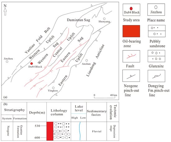
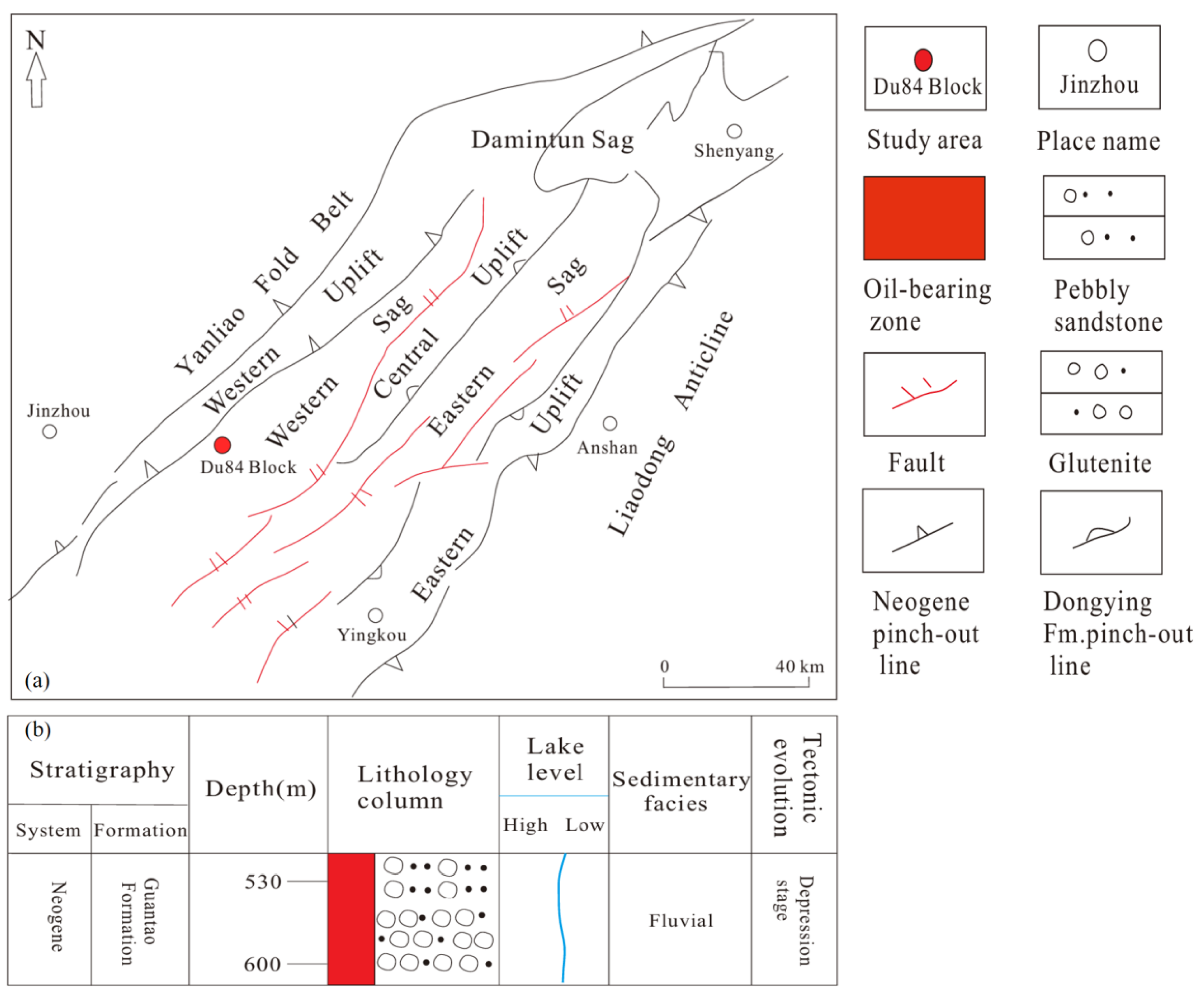
The studied interval belongs to the Guantao Formation in the D84 Block (Figure 1). Published descriptions identify coarse clastic deposits, including glutenite, pebbly sandstone, and medium- to coarse-grained sandstone, interbedded locally with finer-grained material. These lithological variations are relevant when interpreting differences between specimens, because plugs from different depths may also represent different grain-size distributions, depositional units, and post-depositional histories. The sampling depths and lithological characteristics of the four investigated samples are summarized in Table 1.
Figure 1.
(a) Tectonic map of the Liaohe Depression showing the location of the D84 Block; (b) Composite stratigraphic column of the Guantao Formation in the study area (modified after [32]).
Table 1.
Basic parameters of the four plug samples from the Guantao Formation, D84 Block.
The D84 Block is reported as an extra-heavy-oil reservoir with relatively high porosity and permeability in portions of the Guantao Formation. Published and field descriptions of the thermal-recovery setting emphasize geological heterogeneity as a challenge for the interpretation of fluid migration and steam-chamber development [2,6,9,28,29,30]. The D84 Block has also been reported to exhibit H2S generation during thermal recovery, which is relevant to production safety and reservoir fluid chemistry [33]. This study does not simulate steam, heat transfer, or multiphase displacement; its calculations address only single-phase flow through the segmented digital pore volumes.
2.2. Samples and CT Scanning
Four plug samples, ZS-1 through ZS-4, were obtained from well D84-X in the Guantao Formation. Their sampling depths are 562.61, 575.63, 592.97, and 625.44 m, respectively. According to the sampling records, ZS-1 was obtained from the upper asphalt-shell interval, ZS-2 from the transition interval, and ZS-3 and ZS-4 from the principal steam-chamber interval. Lithological classifications, physical porosity, measured permeability, and nominal plug dimensions are listed in Table 1. ZS-1 and ZS-3 are described as oil-bearing or oil-impregnated glutenite, respectively, while ZS-2 and ZS-4 are oil-impregnated pebbly medium- to coarse-grained sandstone. The plug samples were imaged in their original oil-impregnated state; the pore space therefore contained residual heavy oil rather than being air-filled. This condition should be considered when interpreting grayscale contrasts, because oil-filled voids attenuate X-rays more strongly than empty pores. The measured porosity and permeability were determined by overburden-pressure core analysis in accordance with SY/T 6385-2016, using an intelligent overburden porosity–permeability measurement system (No. 130703). Nitrogen was used as the testing gas (gas viscosity 0.018 mPa·s) at an upstream pressure of approximately 1.2 atm, with confining pressures ranging from 2.76 to 7.07 MPa and a laboratory temperature of approximately 23–25 °C. The permeability was measured along the plug axis. The test report did not document a separate gas-slip (Klinkenberg) correction or an explicit measurement uncertainty; the values are therefore reported as measured under the stated pressure and confining-stress conditions. The sampling depth, lithological description, and nominal plug dimensions were taken from the coring and core-description records. The CT-derived porosity and simulated permeability listed in Table 1 were obtained as described in Section 2.3.2 and Section 2.3.3. The four plugs were selected to span the principal producing interval of the Guantao Formation in well D84-X, covering a depth range of approximately 63 m and the three recognized development subzones: the upper asphalt-shell interval (ZS-1), the transition interval (ZS-2), and the principal steam-chamber interval (ZS-3, ZS-4). The sample set also includes the two dominant lithofacies of the studied interval, namely glutenite (ZS-1, ZS-3) and pebbly medium- to coarse-grained sandstone (ZS-2, ZS-4). The sampling design therefore captures the documented lithological and zonal variation within the cored interval, rather than treating the specimens as replicates of a single facies.
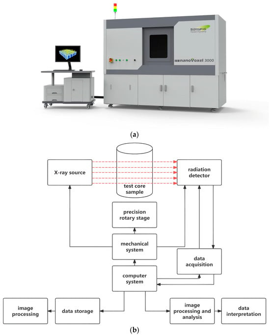
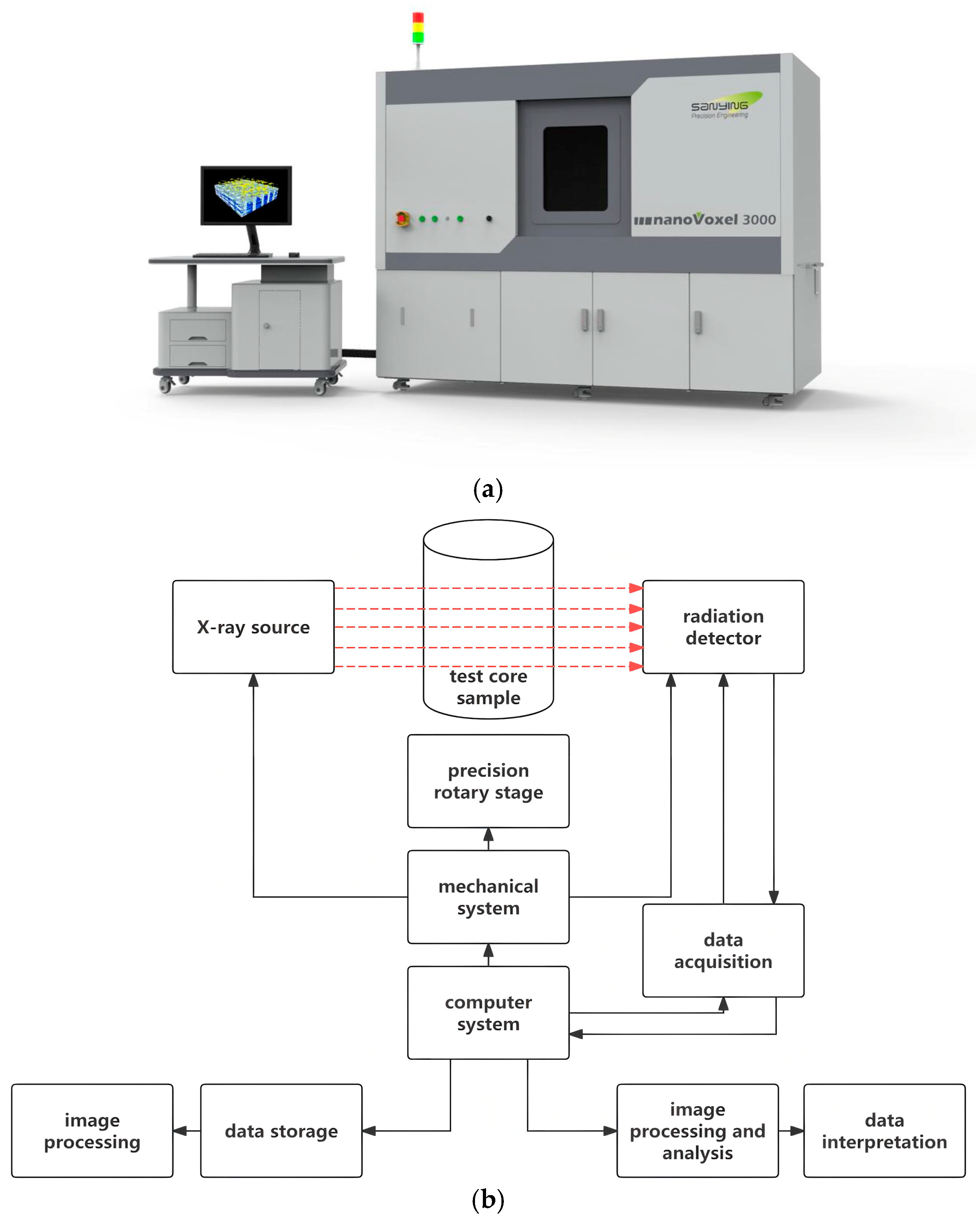
The plugs were imaged using a nanoVoxel-3000 X-ray micro-CT system (Sanying Precision Instruments, Tianjin, China). The samples were scanned at an accelerating voltage of 200 kV and a tube current of 200 μA, with an exposure time of 0.55–0.60 s per projection. A total of 2880 projections were acquired over two rotations. The tomographic volumes were reconstructed using the FDK algorithm with a Hamming filter, followed by median filtering and software-based beam-hardening correction, yielding an isotropic voxel size of approximately 9.37 μm (Figure 2). CT image data were exported in RAW format for further processing. No fracture-like features were identified in the available images at this spatial resolution; this observation does not exclude sub-resolution fractures, nor does CT morphology alone establish the primary or secondary origin of every pore. As image segmentation cannot resolve all fine pores and throats, CT-derived porosity may differ from laboratory porosity. The effect of voxel size should be considered when interpreting the reported small-pore classes [14,34,35].
Figure 2.
(a) The nanoVoxel-3000 micro-CT scanning system; (b) Schematic diagram of the CT imaging principle. In (b), the red dashed arrows indicate the X-ray path from the X-ray source through the sample to the detector, while the solid arrows indicate the control and data-flow connections.
The investigated lithologies include oil-bearing or oil-impregnated glutenite and pebbly medium- to coarse-grained sandstone. The latter category applies to ZS-2 and ZS-4, including ZS-4 at 625.44 m. This lithological variation is retained in sample-level interpretations instead of treating all four plugs as petrographically identical.
2.3. Digital Core Construction and Seepage Simulation Methods
2.3.1. Image Preprocessing and Segmentation
The acquired RAW-format CT images were imported into PerGeos (Thermo Fisher Scientific, Waltham, MA, USA) for preprocessing and three-dimensional digital core reconstruction. Non-local means filtering and grayscale adjustment were applied to improve image quality [36]. Regions affected by imaging artifacts were excluded, while the remaining sample volume was retained for pore structure characterization and subsequent flow simulation. No additional internal subvolume was extracted for the analysis.
Interactive threshold segmentation was employed to distinguish pore space from the solid matrix. The grayscale thresholds were manually adjusted by visually comparing the segmented pore regions and pore–solid boundaries with the original CT images [35]. The final grayscale thresholds were 3500, 5060, 4900, and 4411 for ZS-1 to ZS-4. Laboratory-measured porosity was used as an auxiliary reference for assessing the segmented results rather than as the sole criterion for threshold selection. Specifically, the threshold for each sample was first determined by visually matching the segmented pore–solid boundary to the grayscale transition in the original CT images, without reference to the laboratory porosity. The laboratory-measured porosity was then used only as an independent post-segmentation check that the resulting CT porosity fell within a reasonable range. The segmentation was further validated by (i) inspecting the segmented pore outlines overlaid on the original CT slices, confirming that the boundaries follow the grayscale transition zones, and (ii) the threshold sensitivity analysis, in which the segmentation was repeated at thresholds of −5%, −3%, −1%, +1%, +3%, and +5%; over this range, CT-derived porosity varied by 2.0–3.3 percentage points (a relative change of approximately 7–10%), while the simulated permeability changed by only −2.4% to +0.9% at the ±5% thresholds. A representative original CT section with the segmented pore space overlaid is provided in Supplementary Figure S1, and the complete threshold sensitivity results, including the CT-derived porosity at all seven threshold levels and the simulated permeability at the baseline and ±5% thresholds for each sample, are listed in Supplementary Table S1. The resulting images were converted into binary digital core models, in which pore and solid voxels were assigned values of 1 and 0, respectively.
2.3.2. Pore Structure Parameters and Axial Heterogeneity
The digital cores were characterized using CT-derived porosity, the three-dimensional volumes and equivalent spherical diameters of labeled pore objects, and cross-sectional porosity variability along the sample axis. These complementary descriptors describe the amount of segmented pore space, the sizes of objects identified by the selected labeling rule, and the spatial variation in porosity along the reconstructed volume.
CT-derived porosity was calculated from the binary volume as the ratio of pore voxels to all voxels within the analyzed sample volume [14,15]:
where Np is the number of voxels classified as pore space, and Nt is the total number of voxels in the analyzed volume.
Following threshold segmentation, Label Analysis was applied directly to the binary pore phase in PerGeos, without watershed separation or other pore-body separation procedures. The operation assigns labels to connected voxel objects using a 26-neighbor (face, edge, and corner) connectivity rule. The total numbers of 3D labeled objects were 116,520, 297,054, 300,391, and 383,242 for ZS-1 to ZS-4. Axis Connectivity (26-neighbor) further identified one inlet-to-outlet percolating network in each sample, accounting for 99.90%, 99.81%, 99.80%, and 99.75% of the pore volume. A sample-spanning network is a single, highly branched, non-spherical object that cannot be assigned a physically meaningful pore-scale equivalent diameter (its equivalent diameter would be of the order of the sample dimensions); it is therefore quantified separately as the connected pore fraction and by the permeability, rather than being treated as an individual pore. The remaining 116,519, 297,053, 300,390, and 383,241 objects are discrete pore objects, for which an equivalent spherical diameter is a meaningful size descriptor; these are the objects characterized in the distribution below. For each discrete object, the software-derived equivalent spherical diameter (EqDiameter) and three-dimensional volume (Volume3d) were exported. A labeled connected object is not necessarily identical to an individual geological pore body; accordingly, the statistics below are described as labeled-object descriptors.
The equivalent spherical diameter of labeled object j was calculated from its three-dimensional volume [13,14]:
where Deq,j is the equivalent spherical diameter and Vj is the three-dimensional volume of labeled object j. This definition assigns the diameter of a sphere with the same volume as the object and does not describe the width of a pore throat.
Labeled objects were assigned to the five nominal equivalent-diameter classes used in the original data analysis: 3–30, 30–50, 50–70, 70–90, and >90 μm. The volume fraction for each class was obtained by summing the exported Volume3d values of its constituent objects and dividing by the total Volume3d of all objects included in the analysis [14]:
where Pi denotes the volume percentage of diameter class i, Ci is the set of labeled objects assigned to that class, and n is the number of objects included in the denominator. The numerical classification describes object-equivalent diameters rather than independently resolved pore-body or pore-throat diameters.
To examine heterogeneity along the reconstructed sample axis, the pore-pixel fraction was calculated on successive cross sections normal to the digital-core Z-axis, with a section spacing equal to the voxel size (9.37 μm); no additional averaging or down-sampling was applied between adjacent sections. The resulting sequence was summarized using the coefficient of variation (CV), a normalized measure of the spread of sectional porosities around their mean [14]:
where σφ is the standard deviation of cross-sectional porosity and the mean porosity is the average of the cross-sectional values. The Z-axis refers to the coordinate direction of the reconstructed volume; it is not interpreted as the geological vertical unless sample orientation is independently documented.
2.3.3. Single-Phase Flow Simulation
Single-phase incompressible flow was simulated using the reconstructed digital cores in PerGeos. The principal imaging and model parameters are summarized in Table 2. Water was used as the working fluid, with a dynamic viscosity of approximately 1.0 mPa·s at room temperature. Flow was imposed along the model Z-axis, with an inlet pressure of 130,000 Pa and an outlet gauge pressure of 0 Pa, corresponding to a pressure difference of 0.13 MPa. Solid surfaces were treated as no-slip boundaries, and the lateral faces were assumed to be impermeable.
Table 2.
Parameters for CT image processing and single-phase flow simulation.
The flow was modeled by solving the steady-state incompressible Stokes equations, namely the continuity equation and the momentum equation [13]:
where u is the velocity vector and P is pressure. The equations were solved using a finite-volume method on the Cartesian voxel grid of the segmented images, with a grid spacing of 9.37 μm. A one-voxel boundary layer represented the solid walls, and inlet/outlet extension regions were added to avoid end effects. A target tolerance of 10−6 for the relative variation in the velocity and pressure fields was specified in the solver settings. During the iteration, the monitored normalized residual decreased by more than one order of magnitude and then reached a stable plateau at approximately 0.4%; further iterations did not reduce it because of the geometric complexity of the voxelized pore boundaries. Convergence was therefore assessed using two complementary criteria: the volume-integrated permeability remained essentially unchanged over the plateau, and the inlet and outlet mass flow rates balanced to within approximately 1%. On this basis the solution was treated as converged for the permeability calculation, while the 0.4% residual level defines the numerical precision of the reported fields. The simulated permeability was calculated according to Darcy’s law [13]:
where k is permeability (m2), q is the simulated volumetric flow rate (m3/s), μ is dynamic viscosity (Pa·s), L is the length of the analyzed digital core along the flow direction (m), A is the flow-normal cross-sectional area (m2), and ΔP is the imposed pressure difference (Pa). The sample-specific values of L and A used in Darcy’s law are listed in Table 3. Streamline and pressure fields were exported for qualitative comparison of the numerical flow patterns. The applicability of Darcy’s law was checked by evaluating the imposed pressure gradient and the pore-scale Reynolds number. The pressure gradient was ΔP/L ≈ 13.2 MPa m−1. The corresponding Darcy (apparent) velocities, calculated from v = k∇P/μ, ranged from approximately 13.2 to 19.3 mm s−1, and the interstitial velocities (v/φ) from approximately 47 to 70 mm s−1. Using the pore-scale Reynolds number Re = ρv√k/μ, where √k is the characteristic length scale, the values for the four samples ranged from 0.013 to 0.023. Even when an interstitial velocity and a conservative pore diameter are adopted, the Reynolds number remains of order 1 to a few, which is still well within the steady laminar regime and far below the onset of turbulence. The flow is therefore in the low-Reynolds-number, viscosity-dominated laminar regime, for which the Stokes equations and Darcy’s law are valid.
∇·u = 0
−∇P + μ∇2u = 0
The simulated permeabilities were compared with laboratory measurements to evaluate the differences between the numerical and experimental results. The relative difference was calculated as [14]:
3. Results
3.1. Three-Dimensional Pore Morphology and CT-Derived Porosity
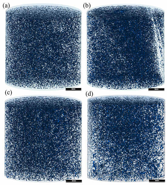
The segmented micro-CT volumes and their three-dimensional pore visualizations are displayed in Figure 3. All four samples contain a substantial volume of CT-resolved pore space. No distinct fractures were recognized in the visualizations at the reported voxel size. The images are consistent with a largely granular pore system, but the distinction between primary intergranular pores and other pore types cannot be established unambiguously from these CT renderings alone.
Figure 3.
Three-dimensional pore models of the four plug samples. (a) ZS-1; (b) ZS-2; (c) ZS-3; (d) ZS-4. Scale bar = 5 mm.
The CT-derived porosities ranged from 27.37% to 32.92% (Table 1 and Table 3). ZS-2 and ZS-3 had relatively high values of 32.92% and 32.52%, whereas ZS-1 and ZS-4 had lower values of 27.37% and 28.00%. All CT-derived values were lower than their laboratory counterparts. Although both methods quantify porosity, they are not strictly equivalent: the CT result is obtained from an artifact-filtered, segmented image volume, whereas laboratory porosity represents the material and measurement conditions used in conventional core analysis.
The difference between the highest and lowest CT porosity was 5.55 percentage points (ZS-2 minus ZS-1), whereas the range of measured porosity was 7.8 percentage points (35.8% in ZS-3 versus 28.0% in ZS-1). The ranking by total pore fraction was not identical between the two measurement approaches. In particular, ZS-3 had the highest laboratory porosity, while ZS-2 had the highest image-derived porosity. These descriptive contrasts make it useful to report both sets of measurements rather than treating them as interchangeable.
The absolute laboratory-minus-CT porosity differences were 0.63, 2.28, 3.28, and 3.80 percentage points for ZS-1 through ZS-4, respectively, corresponding to relative differences of approximately 2.2%, 6.5%, 9.2%, and 11.9%. These differences may reflect unresolved fine pores, segmentation choices, and differences between the volumes and conditions represented by the methods. Laboratory porosity was used as an auxiliary visual-segmentation reference rather than as a wholly independent verification dataset; apparent agreement in total pore fraction cannot by itself verify pore geometry. The porosity range of the four samples is consistent with high-porosity, high-permeability Guantao Formation reservoirs reported elsewhere. For example, the fine-sandstone facies of point-bar sand bodies in the Guantao Formation of Gudao Oilfield has porosities of 28–37% (mean 34.2%) [37]. In contrast, the CT-derived porosities here are markedly higher than those of deep glutenite reservoirs, such as the ultra-low-porosity glutenite in Bozhong Sag (2.86–17.70%, mean 9.61%) [38] and the low-permeability Sangonghe Formation samples in Mobei Oilfield (10.2–14.4%) [39]. These comparisons indicate that the four plugs are high-porosity, shallow Guantao Formation samples rather than deep tight glutenite.
Table 3.
Summary of pore structure characterization and simulation results.
Based on CT porosity, ZS-2 and ZS-3 form a higher-porosity pair, while ZS-1 and ZS-4 exhibit lower values. These groups are descriptive comparisons within the four analyzed specimens and are not intended as statistically defined reservoir classes.
For example, ZS-2 and ZS-3 have closely comparable CT porosities (32.92% and 32.52%) yet different axial porosity CV values (6.19% and 7.98%). Similarly, ZS-1 and ZS-4 have similar CT porosities (27.37% and 28.00%) but simulated permeabilities differing by 468 mD. These comparisons suggest that a single bulk porosity number cannot reproduce all structural and modeled-flow differences, without isolating which specific geometric characteristic is responsible.
3.2. Equivalent Diameter Distribution of Discrete Pore Objects
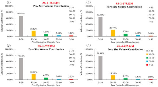
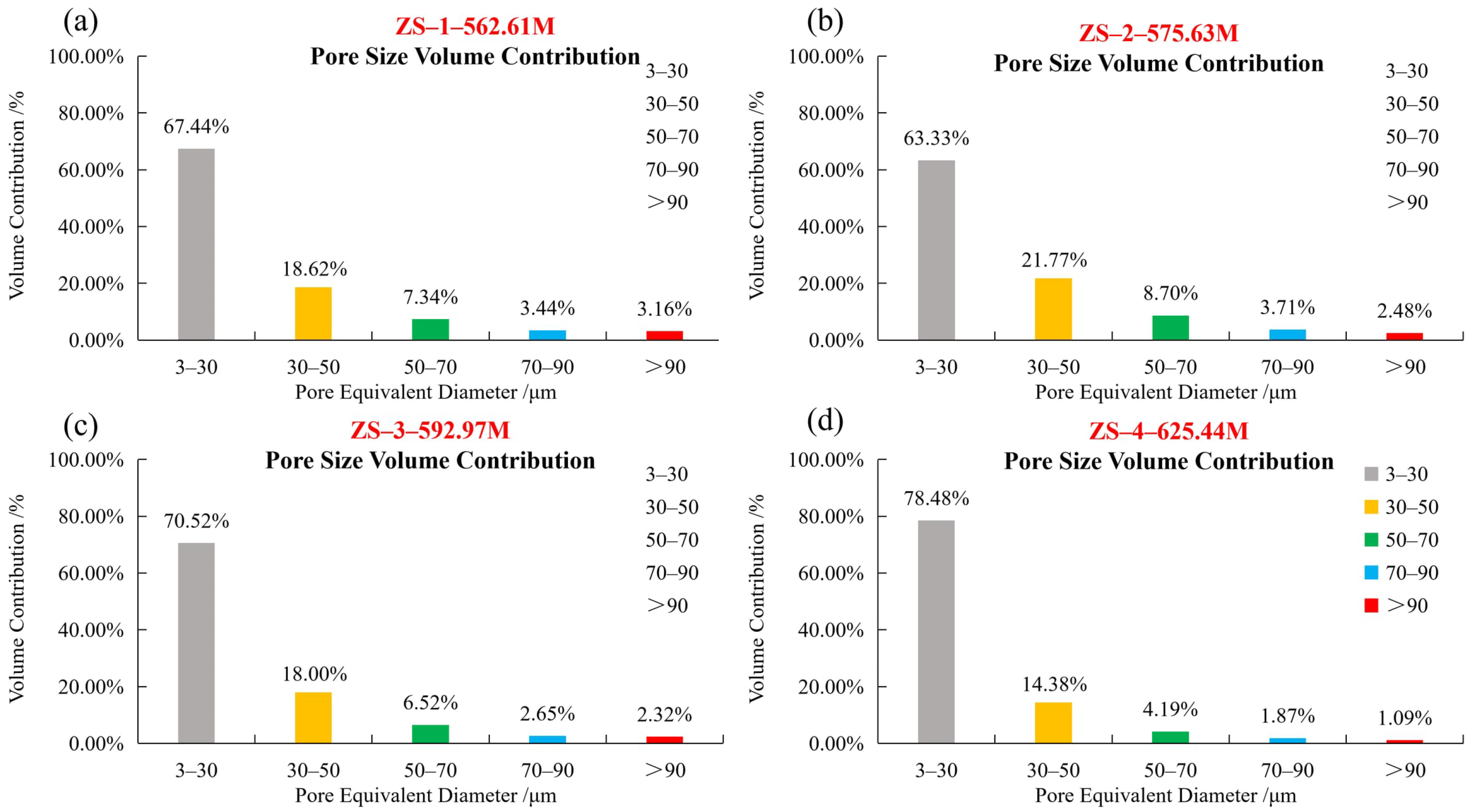
Figure 4 presents the volume-weighted equivalent-diameter distributions of the labeled pore objects in the four digital cores. The nominal diameter classes were 3–30, 30–50, 50–70, 70–90, and >90 μm. The corresponding volume fractions were 63.33–78.48%, 14.38–21.77%, 4.19–8.70%, 1.87–3.71%, and 1.09–3.16%, respectively. The 3–30 μm class accounted for the largest reported volume fraction in all four samples.
Figure 4.
Volume-weighted equivalent-diameter distributions of the discrete labeled objects only (excluding the sample-spanning percolating network) in the four plug samples. (a) ZS-1; (b) ZS-2; (c) ZS-3; (d) ZS-4.
Because the calculation is volume weighted, the contribution of a size class reflects the sum of the labeled-object volumes assigned to that interval, not the number percentage of objects. A class containing fewer but larger labeled objects can therefore account for more total volume than a class containing many small objects. This distinction is important when comparing the four distributions and avoids interpreting the reported percentages as object-count frequencies.
An equivalent diameter is a convenient scalar summary of a three-dimensional object, but two objects with the same volume and diameter can have very different shapes. In particular, a branched connected object and a compact nearly spherical object can share the same equivalent spherical diameter. The class fractions therefore should not be read as measurements of pore shape, pore-throat width or conductance. Those would require other image-analysis operations beyond the labeled-object volume measurements used here.
The equivalent-diameter distributions varied among the four samples. ZS-4 exhibited the highest volume fraction in the 3–30 μm class (78.48%) and the lowest fraction in the >90 μm class (1.09%). ZS-2 had the lowest fraction in the 3–30 μm class (63.33%) and the highest fraction in the 30–50 μm class (21.77%). ZS-1 showed the highest fraction in the >90 μm class (3.16%). These results describe differences in the equivalent-diameter composition of the labeled pore objects among the samples. It should be noted that these distributions characterize only the discrete labeled objects, which together account for 0.10–0.25% of the total pore volume; the sample-spanning percolating network that occupies the remaining 99.75–99.90% is reported separately (Section 2.3.2). The percentages below therefore describe the composition of the discrete objects rather than the bulk pore system. The dominance of the 3–30 μm class and the relatively large pore scale here are consistent with the high-porosity samples. In comparison, the low-permeability Sangonghe Formation digital cores (imaged at 2.68 μm) had a mean pore radius of 33.11 μm but a much smaller mean throat radius of 1.47 μm, and the narrow throats were identified as the main cause of their low permeability [39]. This contrast suggests that the present samples contain larger, better-connected pore spaces than low-permeability glutenite.
The combined volume fractions of labeled pore objects with equivalent diameters greater than 50 μm were 13.94%, 14.89%, 11.49%, and 7.15% for ZS-1 through ZS-4, respectively (Table 3). ZS-2 showed the highest fraction in this combined class, while ZS-4 exhibited the lowest. No monotonic variation with sampling depth was observed for this parameter.
The nominal class boundaries were applied consistently to the reported datasets. The combined >50 μm fraction provides a convenient summary of the upper three classes, but it was not selected as a tested hydraulic cutoff. Thus, differences in this fraction are reported as differences in labeled-object equivalent-diameter composition only.
The descriptive ordering is also not the same for every summary statistic. Although ZS-2 had the greatest combined fraction above 50 μm, ZS-1 had the largest fraction in the >90 μm class. Combining several bins thus changes the ranking because the groups summarize different parts of the labeled-object volume distribution. For this reason, the paper retains the original five-class distributions alongside the condensed >50 μm fraction instead of using a single threshold as a substitute for the entire distribution.
3.3. Axial Porosity Variation Along the Sample Length
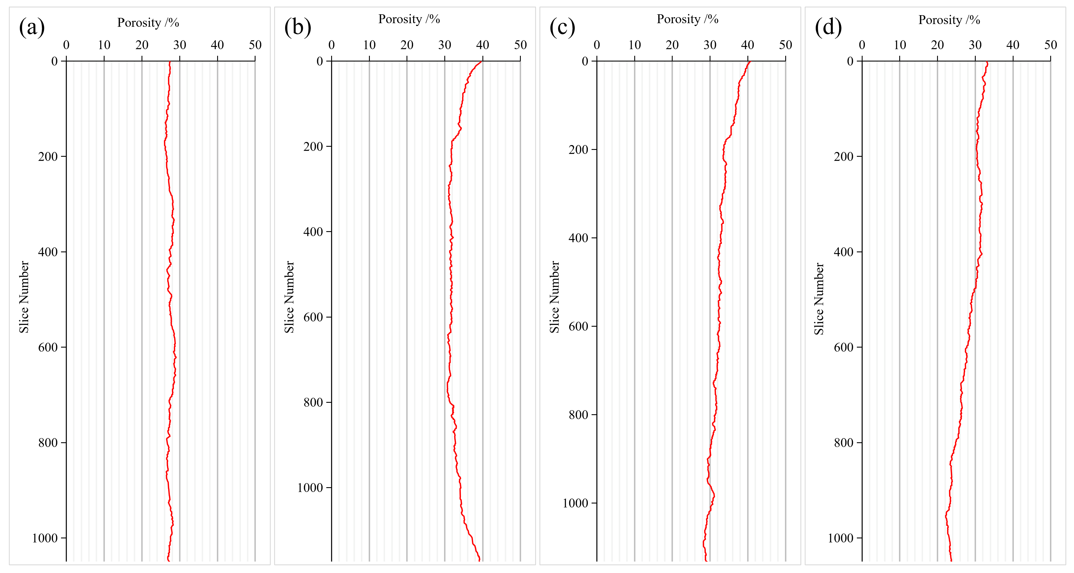
Figure 5 shows the variation in CT-derived section porosity along the digital-core Z-axis. The profiles fluctuate around different mean values and show visibly different amplitudes and patterns. Since these are successive cross sections within single reconstructed plugs, they represent within-plug axial variability, not a direct measurement of field-scale reservoir heterogeneity or a laterally continuous geological vertical profile. It should be noted that only a section of each plug was scanned rather than the entire 25 mm plug; regions affected by imaging artifacts were subsequently cropped. The analyzed section was therefore approximately 10 mm in length along the flow direction, with the cross-sectional area taken from the cropped sample face. These physical dimensions (L and A) were used in Darcy’s law.
Figure 5.
Variation in CT-derived porosity along the sample length (a) ZS-1; (b) ZS-2; (c) ZS-3; (d) ZS-4.
For each section, the plotted porosity represents the fraction of pore pixels in the analyzed cross-sectional mask. Variations along Z therefore describe the distribution of segmented void space within a single digital specimen. They should not be conflated with a field-scale vertical porosity log or a direct measure of preferential hydraulic paths.
For example, a constant average pore fraction along the sample can coexist with localized higher- and lower-porosity sections; conversely, a smooth profile does not establish that void space is hydraulically continuous between sections. As a normalized statistic, CV allows the fluctuation amplitude to be viewed relative to each specimen’s mean porosity. It does not, however, provide an absolute length scale for the heterogeneity, and differences in section spacing or masking choices could change the reported profile. Because the section spacing equals one voxel, the profiles retain the short-scale porosity fluctuations, whereas a coarser spacing would smooth these fluctuations and bias the CV downward. All four samples were analyzed with the same one-voxel spacing, so their relative CV comparison remains valid. The comparison is therefore restricted to the reported analysis axis and reconstruction procedure.
The coefficients of variation (CVs) of cross-sectional porosity were 2.48%, 6.19%, 7.98%, and 11.74% for ZS-1 through ZS-4, respectively (Table 3). ZS-1 displayed the smallest fluctuation relative to its mean porosity, whereas ZS-4 displayed the largest. The CVs increased in the same order as the four sampling depths. This observed ordering does not, by itself, identify burial depth or thermal recovery as the cause. Moreover, lithology and development-zone position also change along the depth sequence, so depth cannot be treated as an independent controlling variable.
ZS-2 and ZS-3 illustrate the added information provided by axial profiles. Despite mean CT porosities of approximately 33%, their respective CVs were 6.19% and 7.98%, demonstrating that similar whole-volume pore fractions may coexist with different section-by-section variations. The axial profiles therefore complement, rather than replace, volume-average porosity in describing the reconstructed images.
The section-wise CV describes variation along one digital-core axis; it is not a direct measurement of three-dimensional pore-throat continuity, hydraulic tortuosity, or anisotropy. Since the samples also vary in lithology and stratigraphic position, comparison among the four CV values is descriptive and does not isolate an independent geological control.
3.4. Simulated Permeability and Single-Phase Flow Distribution
Single-phase simulations yielded permeabilities of 1477, 1183, 1176, and 1009 mD for ZS-1 to ZS-4, respectively (Table 3; Figure 6a). The values span 1009–1477 mD, with ZS-1 highest and ZS-4 lowest in the simulated set. Because the pore-space models are based on segmented CT images, these estimates should be interpreted as model-dependent absolute permeabilities rather than direct measurements of reservoir-condition multiphase flow.
The simulations used a consistent pressure difference of 0.13 MPa to generate a steady single-phase response in the reconstructed geometries. The corresponding permeability values are derived from flow rate and Darcy’s law, rather than obtained by fitting the experimental permeabilities. They therefore permit an informative comparison of numerical outcomes, while differences in segmentation and laboratory conditions remain relevant to interpretation.
Darcy permeability is computed from the integrated response of the numerical domain and does not by itself reveal which local features dominate the pressure loss. The streamline panels provide a complementary visual depiction of solution trajectories, while the pressure panels show how the imposed pressure condition is distributed within the model. Their interpretation is strongest when used to illustrate the computed field rather than to infer unmeasured connected volume or specific throat conductance.
Figure 6.
(a) Comparison of measured and CT-simulated permeability; (b) Comparison of measured and CT-derived porosity.
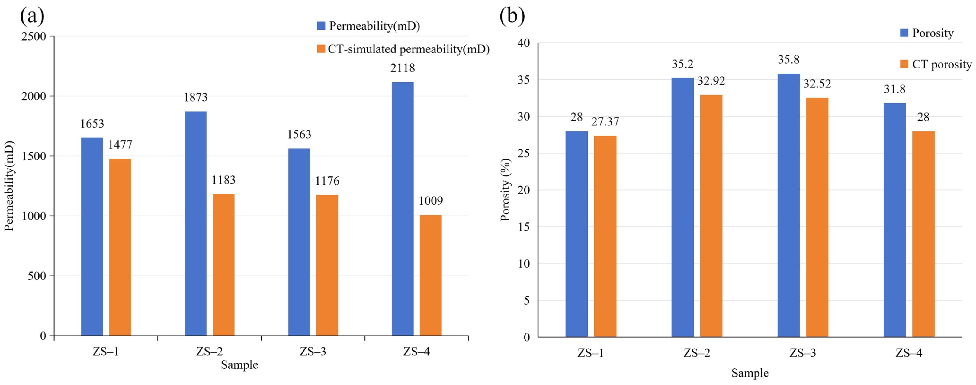
The simulated permeabilities were lower than the corresponding laboratory-measured values for all four samples. The relative differences were −10.6%, −36.8%, −24.8%, and −52.4% for ZS-1 through ZS-4, respectively, with a mean absolute percentage difference of approximately 31.2%. ZS-4 exhibited the largest discrepancy, with a simulated permeability of 1009 mD compared with the measured value of 2118 mD. The simulated permeabilities (1009–1477 mD) are consistent with those of the fine-sandstone facies in the Guantao Formation of Gudao Oilfield (800–3000 mD, mean 1350 mD) [37] and are far above those of deep tight glutenite in Bozhong Sag (0.03–425.93 mD) [38]. The systematic underestimation relative to measurements (mean absolute difference 31.2%) is also consistent with the digital-core results of Qu et al. [39], who found that simulated permeabilities were generally lower than measured values, with a relative error of 33.8%.
The laboratory-measured permeabilities decreased in the order ZS-4 > ZS-2 > ZS-1 > ZS-3, whereas the simulated values followed the order ZS-1 > ZS-2 > ZS-3 > ZS-4. The differences in both magnitude and ranking indicate that the simulations did not fully reproduce the variations observed in the laboratory measurements. The results therefore represent model-dependent permeability estimates rather than an independently validated prediction of experimental permeability.
The comparison also shows that ZS-2 and ZS-3 differed by only 7 mD in simulated permeability (1183 and 1176 mD). Such a small difference should not be interpreted as a physically meaningful separation without numerical uncertainty estimates. The primary result is the broader pattern of disagreement between simulated and measured magnitudes and sample ordering, rather than the exact ranking of nearly equal modeled values.
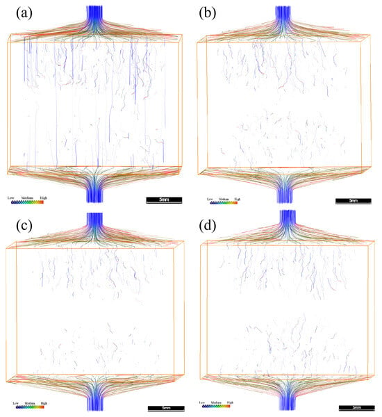
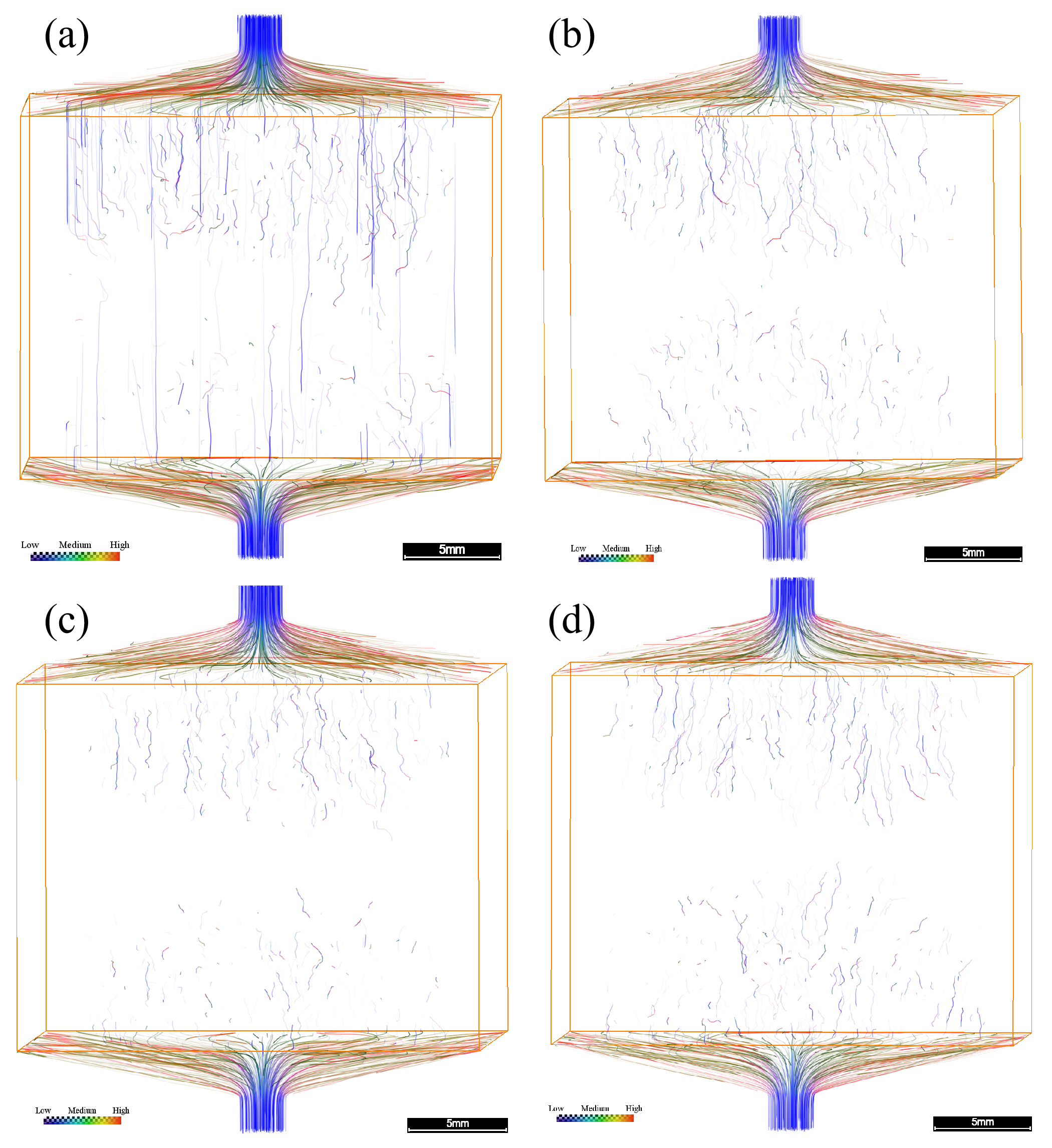
Figure 7 presents the simulated streamline distributions in the four digital cores. Differences in streamline patterns and spatial distributions were observed among the samples, providing a qualitative visualization of the simulated single-phase flow fields. The streamlines were generated using the same seed-point settings for all four samples (an identical number of uniformly distributed seeds), so the streamline panels are intended for a qualitative comparison of flow-path distribution. Streamlines trace the trajectories of fluid particles in the steady-state flow field, with color encoding the local velocity magnitude (blue = low, through green/yellow, to red = high). Driven by the imposed pressure difference, fluid enters through the top inlet and exits through the bottom outlet. The density, continuity, and tortuosity of the streamlines reflect the connectivity and hydraulic resistance of the pore network. The four samples show distinct patterns. ZS-1 has the greatest number of continuous, through-going streamlines, with several nearly straight vertical paths that indicate well-connected preferential flow routes and relatively low overall resistance; this is consistent with ZS-1 having the highest simulated permeability. ZS-2 shows fewer, moderately distributed streamlines, while ZS-3 and ZS-4 show the sparsest, most tortuous, and least continuous paths, indicating poorer connectivity and higher resistance; ZS-4 in particular has few continuous through-going routes despite having a porosity similar to ZS-1. These patterns suggest that the modeled permeability is governed primarily by pore connectivity and the availability of continuous flow paths rather than by total porosity alone, which helps explain why samples with similar bulk porosities (e.g., ZS-1 and ZS-4) can have markedly different simulated permeabilities.
Figure 7.
Streamline distributions of the four plug samples (a) ZS-1; (b) ZS-2; (c) ZS-3; (d) ZS-4. The streamline color indicates relative velocity along the streamlines (blue = low, red = high); the plot is a qualitative visualization of the flow trajectories rather than a quantitative velocity field. Scale bar = 5 mm.
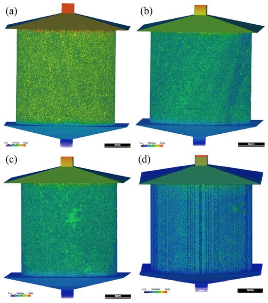
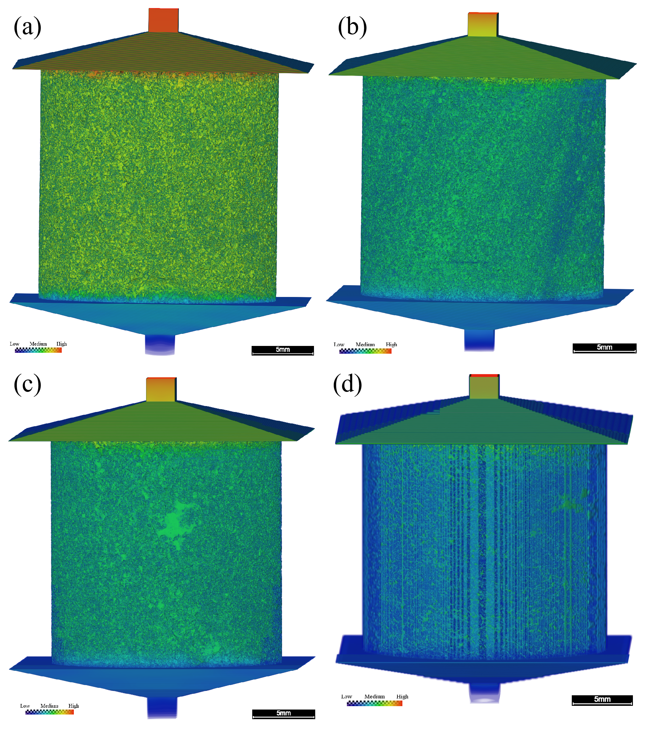
Figure 8 shows the simulated pressure distributions under the imposed inlet–outlet pressure difference of 0.13 MPa. The fields illustrate nonuniform pressure variations within each computed domain. All four panels use the same color scale (0–130,000 Pa), so the same color represents the same pressure in every sample and the panels are quantitatively comparable. The pressure decreases from the inlet to the outlet, with nonuniform local gradients reflecting the underlying pore geometry.
Figure 8.
Pressure field distributions of the four plug samples (a) ZS-1; (b) ZS-2; (c) ZS-3; (d) ZS-4. Scale bar = 5 mm. The color scale is identical for all four panels, ranging from 0 Pa (Low) to 130,000 Pa (High).
4. Discussion
4.1. Comparison of Pore Structure Characteristics and Simulated Flow
The CT-derived descriptors address complementary properties of the reconstructed pore space. Whole-volume porosity measures the fraction of voxels classified as void, whereas equivalent-diameter statistics summarize the volumes of the objects identified by the image-labeling procedure. Axial porosity CV describes the variation in the segmented pore fraction between successive sections. None of these individual measures directly represents the full hydraulic geometry of a connected flow pathway, but together they permit more informative comparisons of the four specimens than a single porosity value.
The porosity–permeability comparison emphasizes this distinction. ZS-1 had the lowest CT porosity (27.37%) but the highest computed single-phase permeability (1477 mD). In contrast, ZS-2 and ZS-3 had higher CT porosities (32.92% and 32.52%) and lower simulated permeabilities (1183 and 1176 mD). Thus, CT porosity alone does not determine the permeability ordering within these models. In porous media, flow also depends on the arrangement and hydraulic conductance of pathways [13,14,27]. The present calculations do not separately quantify throat connectivity, coordination number, or tortuosity, so these mechanisms remain background explanations rather than experimentally established sample-specific controls.
The reported equivalent-diameter composition offers a second contrast. For the nominal classes above 50 μm, the reported volume fractions were 13.94%, 14.89%, 11.49%, and 7.15% for ZS-1 to ZS-4, respectively. ZS-2 had a slightly higher fraction than ZS-1, although ZS-1 displayed a higher simulated permeability. Conversely, ZS-4 showed the smallest fraction in these classes and the lowest simulated permeability. Together, the comparisons do not support a simple one-to-one correspondence between this arbitrarily selected 50 μm class boundary and flow capacity. The class threshold is a descriptive bin edge, not an experimentally calibrated boundary between hydraulically effective and ineffective pores.
Axial heterogeneity adds a distinct spatial perspective. The CV values increased from 2.48% in ZS-1 to 11.74% in ZS-4, indicating progressively stronger relative variations in cross-sectional porosity across this particular sequence of samples. The end-member specimens also differed in modeled permeability, but a causal relation cannot be isolated from these observations. The samples represent different depths and lithological contexts, and an axial section-porosity statistic neither measures the continuity of paths between sections nor describes their three-dimensional orientation. Accordingly, the CVs should be read as complementary structural descriptions, not as independent predictors of permeability.
A further qualification concerns the physical interpretation of the size statistics. PerGeos EqDiameter was calculated from Volume3d for labeled connected objects identified directly on the segmented pore phase, without separate pore-body partitioning. Where several pore regions are connected, the software may represent them as a single labeled object; its equivalent spherical diameter is therefore not the diameter of each local pore body or throat. In addition, the voxel pitch was 9.37 μm, whereas the smallest reported nominal class begins at 3 μm. Algorithm-derived values at or below the sampling scale do not demonstrate that physical 3 μm pores were resolved. Figure 4 should therefore be interpreted specifically as a distribution of labeled-object equivalent diameters within the resolution and segmentation limits of the CT images.
4.2. Differences Between Simulated and Measured Permeability
The permeability comparison is a useful diagnostic result, but it does not establish independent validation of the image-based model. The calculated single-phase permeabilities ranged from 1009 to 1477 mD, compared with 1563 to 2118 mD for the laboratory measurements. All four numerical values were lower than their measured counterparts. The relative differences were −10.6%, −36.8%, −24.8%, and −52.4% for ZS-1 through ZS-4, respectively, with a mean absolute percentage difference of approximately 31.2%. The two estimates were of a similar order of magnitude, yet their differences were too substantial to support a claim of close quantitative agreement.
The most conspicuous difference occurred in ZS-4: its laboratory permeability was 2118 mD, the largest measured value, whereas its computed permeability was 1009 mD, the smallest simulated value. The laboratory ranking was ZS-4 > ZS-2 > ZS-1 > ZS-3, while the simulation ranking was ZS-1 > ZS-2 > ZS-3 > ZS-4. The mismatch therefore concerns both magnitude and ordering. A uniform multiplier applied to all modeled values would not resolve the ranking difference. This observation is reported as an outcome of the comparison, without attributing it to an unverified single cause. A further point concerns the reversal of the sample ranking. Laboratory permeability is measured on the full 25 mm plug, whereas the simulated value is obtained from a cropped volume of approximately 10 mm. For the most heterogeneous pebbly sample ZS-4, which also has the largest axial porosity CV (11.74%), a 10 mm sub-volume need not contain the same dominant flow pathways as the full plug, so its permeability can differ substantially from the bulk measurement, and rankings based on these sub-volumes are not expected to reproduce the plug-scale ranking. This is consistent with ZS-4 having the largest measured permeability and hence comparatively wide pore constrictions, for which finite-resolution loss of narrow pore constrictions is an unlikely dominant cause of the 52.4% discrepancy. A systematic sub-volume (REV) analysis using several spatially separated sub-volumes is needed to quantify this effect and is identified as a priority for future work.
Several methodological differences could contribute to the discrepancy. Image segmentation represents the pore phase at finite spatial resolution, so narrow passages and mixed pore–solid voxels may be represented differently from their physical counterparts. Artifact-affected portions of the CT images were excluded from the numerical analysis, whereas the laboratory test reflects the specimen and conditions of the conventional measurement. Finally, gas-based laboratory permeability and single-phase water-based numerical permeability are not identical test configurations. Testing pressure, confining stress, fluid properties and possible gas-slip corrections can affect comparability; their individual contributions cannot be quantified from the information available here [13,14,34,35]. Of these factors, the dominant one is the finite voxel resolution: narrow pore constrictions (physical pore throats that are not directly measured by the present method) and mixed pore–solid voxels that are only a few voxels across tend to be classified as solid. The contribution of segmentation can be quantified through the sensitivity analysis: a ±5% change in the threshold changed the simulated permeability by less than 2.5% across the four samples (Section 2.3.1). In addition, the gas-based laboratory measurement may be biased upward by the Klinkenberg gas-slip effect, whereas the numerical model uses idealized boundaries and a cropped volume rather than the full plug under confining stress. These effects act in the same direction (toward a lower simulated value), except for the stress effect, which is comparatively small. They cannot be fully separated from the present data and would require a dedicated controlled study.
The laboratory porosity values were used only as auxiliary references during visual adjustment of the interactive segmentation threshold. Therefore, the relatively modest laboratory–CT porosity differences do not constitute independent evidence that all hydraulically significant pathways were segmented accurately. A model may reproduce a similar total pore fraction and still represent constrictions or connections differently. Likewise, the simulated flow fields describe transport within the adopted binary geometry rather than directly measuring the permeability of the entire physical plug.
Taken together, the comparison supports reporting the modeled permeabilities as sample-specific numerical estimates alongside their experimental counterparts. The study does not calibrate a reservoir-wide permeability relation, and the observed differences should remain explicit rather than be absorbed into an unexplained correction factor. Further checks of input geometry, laboratory conditions and solver settings would be useful if quantitative prediction becomes the objective of a subsequent study.
4.3. Flow-Field Interpretation and Geological Context
Figure 7 and Figure 8 complement the numerical permeability values by illustrating the computed streamline paths and pressure distributions. Both reflect the imposed steady single-phase problem in the segmented volumes. Streamline maps depend on display and seed-point settings, and pressure plots require consistent scales before visually ranking specimens. Consequently, they are most useful for demonstrating spatially nonuniform numerical fields rather than for quantifying connected pore fraction or identifying a unique constriction in the natural rock.
The geological setting provides a reason to expect variations among the four specimens. Table 1 describes the upper samples and the deeper samples as differing in sampling position and lithological character. In particular, ZS-4 is oil-impregnated pebbly medium- to coarse-grained sandstone, and the specimens should not be treated as lithologically identical replicates. Differences in grain size, grain packing, matrix proportion, deposition and diagenetic history could contribute to structural contrasts. However, these processes were not independently measured or isolated in the present analysis, and the observed differences cannot be assigned to any one of them.
The practical contribution of this work is a coordinated description of image-resolved pore fraction, labeled-object equivalent diameter, axial porosity variability and simulated single-phase flow for samples from the D84 Block. CT-derived descriptors and experimental core analyses illuminate different aspects of the material: imaging permits spatial visualization, while conventional tests provide independent petrophysical measurements under their test conditions. Presenting both, including their disagreements, is more informative than treating either method as an exact substitute for the other.
The scope of the numerical problem must also be distinguished from thermal recovery at reservoir scale. The model assumes single-phase incompressible flow under a prescribed pressure difference; it does not incorporate steam injection, temperature-dependent heavy-oil viscosity, phase saturation, relative permeability, gravity-driven displacement or heat transfer. Hence the computed streamlines should not be identified with steam-chamber pathways, and the calculated permeabilities do not predict SAGD production performance.
Although the present simulations do not reproduce thermal recovery, the plug-scale results can still provide a useful basis for reservoir-scale assessments. The quantified pore-size composition, axial porosity variation, and modeled single-phase permeability constrain the spatial distribution of storage and flow capacity within the sampled facies and can help identify intervals prone to preferential flow or poor sweep. Such pore- and core-scale descriptors serve as inputs for subsequent upscaling steps, including pore-network and relative-permeability modeling at the core scale and integrated geological–reservoir modeling at the field scale. A complete pore-to-reservoir upscaling workflow would require (i) multiphase and thermal-property measurements, (ii) pore-network or relative-permeability models that bridge the pore and core scales, and (iii) integration of the upscaled properties into field-scale thermal reservoir simulations. The present study addresses only the first, pore-scale component of this chain and does not itself perform field-scale upscaling; therefore, the results should be treated as a descriptive pore-scale basis rather than as a direct input to CSS or SAGD design decisions.
Finally, the number and origin of specimens limit the reach of geological interpretation. Four plugs from one well provide a descriptive cross-sample comparison, not a statistically representative survey of the reservoir. Accordingly, the results are intended to characterize pore structure and flow behavior at the plug scale and to illustrate the range of variation among the sampled facies; they are not presented as a statistically representative estimate of the areal or volumetric distribution of properties across the entire D84 Block. Reservoir-wide generalization would require multi-well sampling and an independent, statistically designed sampling program. Their sampling depth, lithology and development-zone assignment vary together, with no controlled pre- and post-heating observations. The observed increase in axial porosity CV across the four depths therefore cannot be taken as evidence of a burial or steam-treatment mechanism. Broader inferences would require replicated sampling and independent geological controls.
The main analytical limitations are finite voxel size, dependence on visual thresholding, uncertainty regarding the relation between labeled objects and individual pore bodies, and imperfect equivalence between the digital model and laboratory measurement configurations. These qualifications do not invalidate descriptive reporting of the acquired results. They do, however, define the appropriate level of inference: the current dataset characterizes four specific digital cores and their numerical single-phase response, rather than establishing a general pore-network mechanism or predictive field-scale model.
5. Conclusions
This study characterized the CT-resolved pore structure and single-phase flow behavior of four Guantao Formation plugs from the D84 Block using 9.37 μm-voxel micro-CT, interactive segmentation, and PerGeos flow simulation. The conclusions are limited to the analyzed samples.
- (1)
- CT-derived porosity ranged from 27.37% to 32.92%, consistently below laboratory porosity. The 3–30 μm labeled-object class accounted for 63.33–78.48% of labeled-object volume and the combined >50 μm classes for 7.15–14.89%; these values describe labeled segmented objects rather than independently separated pore bodies and are resolution-limited by the 9.37 μm voxel size.
- (2)
- Axial porosity CVs were 2.48%, 6.19%, 7.98%, and 11.74%, and simulated single-phase permeabilities were 1477, 1183, 1176, and 1009 mD for ZS-1 to ZS-4. ZS-1 combined the lowest CT porosity with the highest simulated permeability, indicating that bulk porosity alone does not determine the modeled permeability; the qualitative flow patterns suggest that connectivity and the availability of continuous flow paths, rather than bulk porosity, influence the modeled permeability, although this could not be quantified without throat-scale and pore-network analysis.
- (3)
- Simulated permeabilities were lower than measured values for all four samples (absolute relative differences of 10.6–52.4%, mean ≈31.2%), including a ranking mismatch, so the numerical estimates were not independently validated by this comparison. The results provide a sample-scale descriptive basis for integrating CT characterization with flow assessment; further method verification and broader sampling are needed for reservoir-scale application.
Supplementary Materials
The following supporting information can be downloaded at: https://www.mdpi.com/article/10.3390/app162110957/s1, Figure S1: Segmentation overlay for sample ZS-2: (left) original grayscale CT section; (right) the same section with the segmented pore space overlaid in blue. The 5 mm scale bar applies to both panels.; Table S1: Threshold sensitivity of (a) CT-derived porosity (seven threshold levels) and (b) simulated absolute permeability (±5% threshold levels).
Author Contributions
Conceptualization, Y.X. and T.L.; methodology, Y.X. and Y.W.; software, Y.X.; validation, W.H. and H.C.; formal analysis, Y.X. and C.W.; investigation, Y.X., Y.W. and C.W.; resources, T.L. and Y.W.; data curation, Y.X. and P.H.; visualization, S.L. and P.H.; writing—original draft preparation, Y.X.; writing—review and editing, T.L., W.H. and C.W.; supervision, W.H. and T.L.; project administration, T.L. All authors have read and agreed to the published version of the manuscript.
Funding
This research received no external funding.
Data Availability Statement
The underlying datasets are subject to restrictions due to the proprietary nature of the reservoir characterization data. The processed results supporting the findings of this study are presented in the article. Access to additional data is subject to approval by the data owner.
Acknowledgments
The authors thank Jianjun Lei and Zhiqiang Hu for their contributions to the on-site CT scanning work, as well as the anonymous technical team for their support during CT data acquisition and processing.
Conflicts of Interest
Authors Hua Chai, Ping He, Chenglin Wang, and Su Lv were employed by the company Wuhan Zhongwang Yineng Technology Development Co., Ltd. The remaining authors declare that the research was conducted in the absence of any commercial or financial relationships that could be construed as potential conflicts of interest.
Abbreviations
The following abbreviations are used in this manuscript:
| CT | Computed Tomography |
| SAGD | Steam-Assisted Gravity Drainage |
| CSS | Cyclic Steam Stimulation |
| MIP | Mercury Intrusion Porosimetry |
| NMR | Nuclear Magnetic Resonance |
| SEM | Scanning Electron Microscopy |
| ROI | Region of Interest |
| CV | Coefficient of Variation |
References
- Chen, X.; Shao, J.; Sun, Z.; Han, H.; Guo, Q.; Yin, Y.; Sun, X. Characteristics and Controlling Factors of Heavy Oil Distribution in Liaohe Depression, Bohai Bay Basin. Pet. Geol. Exp. 2023, 45, 317–326. [Google Scholar] [CrossRef]
- Li, C.; Fan, T.L.; Gao, Z.Q.; Qian, X.H.; Fu, W. High-Resolution Sequence Stratigraphic Analysis of Alluvial Fans: A Case Study of the Guantao Formation in the SAGD Development Area of Du 84 Block, Shuyi District, Liaohe Depression. Lithol. Reserv. 2017, 29, 66–75. [Google Scholar] [CrossRef]
- Cai, Y.; Fan, Z. Characteristics and genesis of edge and top water extra-heavy oil reservoir in Liaohe Oilfield. Lithol. Reserv. 2011, 23, 129–132. [Google Scholar]
- Jiang, Q.; You, H.; Pan, J.; Wang, Z.; Gai, P.Y.; Gates, I.; Liu, J.L. Preliminary discussion on current status and development direction of heavy oil recovery technologies. Spec. Oil Gas. Reserv. 2020, 27, 30–39. [Google Scholar] [CrossRef]
- Yang, L. Field test of SAGD as follow-up process to CSS in Liaohe oil field of China. J. Can. Pet. Technol. 2007, 46, 35–40. [Google Scholar] [CrossRef] [Scilit]
- Li, Y. Field test analysis of nitrogen assisted SAGD production technology in D84 Block. Pet. Geol. Eng. 2013, 27, 63–65. [Google Scholar]
- Wang, Q.; Yang, H.; Liu, J.; Gao, Y.; Gao, L. Optimization of SAGD key parameters for vertical assisted double horizontal wells in extra-heavy oil reservoir. J. Southwest Pet. Univ. (Sci. Technol. Ed.) 2023, 45, 81–87. [Google Scholar]
- Lu, T.; Ban, X.; Li, Z.; Gao, Y.; Guo, E.; Yang, J.; Ma, H.; Wang, H.; Wei, Y. Mechanism of flue gas assisted SAGD steam chamber expansion. Acta Pet. Sin. 2021, 42, 1072–1080. [Google Scholar] [CrossRef]
- Hou, G. Factors influencing high production of SAGD horizontal wells and adjustment countermeasures in Guantao Formation of D84 Block. Pet. Geol. Eng. 2019, 33, 64–67. [Google Scholar]
- Lai, J.; Wang, G.; Wang, Z.; Chen, J.; Pang, X.; Wang, S.; Zhou, Z.; He, Z.; Qin, Z.; Huang, T. A review on pore structure characterization in tight sandstones. Earth-Sci. Rev. 2018, 177, 436–457. [Google Scholar] [CrossRef] [Scilit]
- Guan, W.; Cai, W.; Li, Z.; Lu, H. Microscopic characterization and fractal analysis of pore systems for unconventional reservoirs. J. Mar. Sci. Eng. 2024, 12, 908. [Google Scholar] [CrossRef] [Scilit]
- Bera, A.; Shukla, B.; Jogani, D. A perspective review of applications of the computed tomography (CT) scan imaging technique for microscopic reservoir rock characterization. Deep Undergr. Sci. Eng. 2025, 5, 4–27. [Google Scholar] [CrossRef] [Scilit]
- Blunt, M.J.; Bijeljic, B.; Dong, H.; Gharbi, O.; Iglauer, S.; Mostaghimi, P.; Paluszny, A.; Pentland, C. Pore-scale imaging and modelling. Adv. Water Resour. 2013, 51, 197–216. [Google Scholar] [CrossRef] [Scilit]
- Wildenschild, D.; Sheppard, A.P. X-ray imaging and analysis techniques for quantifying pore-scale structure and processes in subsurface porous medium systems. Adv. Water Resour. 2013, 51, 217–246. [Google Scholar] [CrossRef] [Scilit]
- Payton, R.L.; Chiarella, D.; Kingdon, A. An introduction for non-experts on using X-ray micro computed tomography as a tool for pore scale digital subsurface characterisation of siliciclastic materials. Sedimentologika 2024, 2, 1367. [Google Scholar] [CrossRef] [Scilit]
- Liu, W.; Shang, L.; Gao, G.; Li, D.; Wang, M.; Geng, W.; Jia, Q.; Zhang, G.; Zhang, H.; Hao, P.; et al. Microstructure characterization of tight reservoirs using micro-CT and FIB-SEM imaging technology. Front. Earth Sci. 2025, 13, 1551826. [Google Scholar] [CrossRef] [Scilit]
- Dong, H.; Blunt, M.J. Pore-network extraction from micro-computerized-tomography images. Phys. Rev. E 2009, 80, 036307. [Google Scholar] [CrossRef] [Scilit] [PubMed]
- Yu, S.; Mehana, M.; Guiltinan, E.J.; Germann, T.C.; Gross, M.R.; Kang, Q. Quantifying the effect of pore-size dependent wettability on relative permeabilities using lattice Boltzmann simulation. J. Geophys. Res. Solid Earth 2025, 130, e2025JB031392. [Google Scholar] [CrossRef] [Scilit]
- Olhin, A.; Vishnyakov, A. Pore structure and permeability of tight-pore sandstones: Quantitative test of the lattice–Boltzmann method. Appl. Sci. 2023, 13, 9112. [Google Scholar] [CrossRef] [Scilit]
- Wan, Y.; Jia, C.; Zhao, W.; Jiang, L.; Chen, Z. Micro-scale lattice Boltzmann simulation of two-phase CO2–brine flow in a tighter REV extracted from a permeable sandstone core: Implications for CO2 storage efficiency. Energies 2023, 16, 1547. [Google Scholar] [CrossRef] [Scilit]
- Ji, Y.; Zhu, K.; Li, K.; Zhao, C.; Liu, K.; Ning, D.; Liu, X.; Yan, P.; Zhao, S. Study on the microscopic pore structure and seepage mechanism of the Luohe Formation sandstone in the roof of coal seams in the Huanglong Coalfield. Sci. Rep. 2025, 15, 18626. [Google Scholar] [CrossRef] [Scilit] [PubMed]
- Liu, J.; Wang, R.; Song, P.; Li, Y.; Zheng, S. Quantitative characterization and flow simulation of micropore structure in clastic gas reservoirs based on micron CT scanning. ACS Omega 2025, 10, 20686–20700. [Google Scholar] [CrossRef] [Scilit] [PubMed]
- Nurcahya, A.; Alexandra, A.; Akmal, F.; Dharmawan, I.A. The lattice Boltzmann method and image processing techniques for effective parameter estimation of digital rock. Appl. Sci. 2024, 14, 7509. [Google Scholar] [CrossRef] [Scilit]
- Yang, J.; Shan, G.; Wang, Z.; Zhang, Q.; Yang, Y.; Ma, W. Experimental study of distribution and quantitative characterization of discontinuous oil phase based on micro-CT. Front. Earth Sci. 2023, 11, 1117971. [Google Scholar] [CrossRef] [Scilit]
- Wu, J.; Gong, W.; Wang, Q.; He, Y.; Guo, J.; Bao, Y.; Shao, S.; Li, R. Dynamic characterization of microscopic pore structure in medium–high permeability sandstones during waterflooding. Nanomaterials 2025, 15, 747. [Google Scholar] [CrossRef] [Scilit] [PubMed]
- Du, Q.-J.; Zheng, H.-Y.; Hou, J.; Liu, Y.-G.; Sun, J.-F.; Zhao, D. Influence of pore structure heterogeneity on channeling channels during hot water flooding in heavy oil reservoir based on CT scanning. Pet. Sci. 2024, 21, 2407–2419. [Google Scholar] [CrossRef] [Scilit]
- Payton, R.L.; Chiarella, D.; Kingdon, A. The upper percolation threshold and porosity–permeability relationship in sandstone reservoirs using digital image analysis. Sci. Rep. 2022, 12, 11311. [Google Scholar] [CrossRef] [Scilit] [PubMed]
- Sun, Z. Research and application of horizontal well thermal recovery technology for heavy oil reservoir in D84 Block, Liaohe Oilfield. Pet. Geol. Eng. 2012, 26, 76–78. [Google Scholar]
- Jia, X. Fine Reservoir Description and Remaining Oil Distribution Characteristics of D84 Block in Shuyi Area, Western Liaohe Sag. Master’s Thesis, China University of Petroleum (East China), Qingdao, China, 2010. [Google Scholar]
- Wang, L. Research on Remaining Oil Potential Tapping Technology in the Medium-Deep Super Heavy Oil Reservoir of D84 Block, Shuyi area, Liaohe Oilfield. Master’s Thesis, Nanjing University, Nanjing, China, 2010. [Google Scholar]
- Wang, Z.; Tang, H.; Yang, J.; Huang, L. Reservoir pore characteristics based on depositional microfacies control in the Neogene Guantao Formation, Bohai Bay Basin, China. Energies 2022, 15, 2870. [Google Scholar] [CrossRef] [Scilit]
- Li, S.; Liu, J.; Ma, X.; Pang, Q.; Zhao, Z. Characteristics and Exploration Potential of the Whole Petroleum System in the Western Sag of Liaohe Depression, Bohai Bay Basin. Oil Gas. Geol. 2025, 46, 1183–1199. [Google Scholar]
- Hou, G. Discussion on the genesis of H2S in Block D84 of Liaohe Oilfield. Pet. Geol. Exp. 2019, 41, 268–273. [Google Scholar] [CrossRef]
- Iassonov, P.; Gebrenegus, T.; Tuller, M. Segmentation of X-ray computed tomography images of porous materials: A crucial step for characterization and quantitative analysis of pore structures. Water Resour. Res. 2009, 45, W09415. [Google Scholar] [CrossRef] [Scilit]
- Huang, R.; He, J.; Wang, C.; Zhang, J.; Hu, D. Multiscale pore/throat characterization in tight sandstone formation with multi-threshold image segmentation algorithm. Front. Earth Sci. 2025, 13, 1576484. [Google Scholar] [CrossRef] [Scilit]
- Buades, A.; Coll, B.; Morel, J.-M. A non-local algorithm for image denoising. In Proceedings of the 2005 IEEE Computer Society Conference on Computer Vision and Pattern Recognition (CVPR’05), San Diego, CA, USA, 20–26 June 2005; Volume 2, pp. 60–65. [Google Scholar] [CrossRef] [Scilit]
- Chen, Q.; Liu, Y.; Liu, H.; Zhao, M.; Bao, L.; Li, X. Controls of different lithofacies in meandering-river point-bar sand bodies on petrophysical evolution during waterflooding: A case study of the Guantao Formation, Gudao Oilfield. Pet. Sci. Bull. 2026, 11, 1283–1299. [Google Scholar]
- Zhang, T.; Hao, P. Fine characterization of the reservoir space in deep ultra-low porosity and ultra-low permeability glutenite in Bozhong Sag. Bull. Geol. Sci. Technol. 2020, 39, 117–124. [Google Scholar]
- Qu, L.; Sun, W.; Du, H.; Zhang, C.; Jiang, L.; Wei, H. Characterization technique of pore structure by 3D digital core based on CT scanning and its application: An example from Sangonghe Formation of 116 Well Field in Mobei Oilfield. Geoscience 2014, 28, 190–196. [Google Scholar]

Disclaimer/Publisher’s Note: The statements, opinions and data contained in all publications are solely those of the individual author(s) and contributor(s) and not of MDPI and/or the editor(s). MDPI and/or the editor(s) disclaim responsibility for any injury to people or property resulting from any ideas, methods, instructions or products referred to in the content. |
© 2026 by the authors. Licensee MDPI, Basel, Switzerland. This article is an open access article distributed under the terms and conditions of the Creative Commons Attribution (CC BY) license.