A Diagnostic Framework for Assessing Cross-Source Generalization in Materials Informatics: Evidence from 1231 Lightweight Aggregate Experiments Across 78 Sources

Abstract

Predictive models of lightweight aggregate (LWA) properties are renowned for their excellent prediction performance within a single source of data, but their generalization power across multiple literature sources is highly questionable. Examination of 1231 observations of LWAs derived from 78 sources (2004–2026 years) and characterized by 120 attributes showed that the pooled Spearman correlation between particle density and water absorption was equal to −0.397 (N = 631; bootstrap 95% CI = −0.459 to −0.329). While 20 out of 22 observed within-source finite correlations were of the same negative sign as the pooled one, the correlations ranged [−0.987, +0.533]. The considerable variability in both magnitude and sign suggests a Simpson-type aggregation effect where the overall coefficient is masking source-level differences. In the case of the complete-case production dataset (N = 278), the Random Forest algorithm reached a mean 5-fold R² of 0.158 but failed in LOSO generalization (mean R² = −3.345 over nine sources). Imputation of predictors increased the sample size to 693 but degraded the LOSO performance (mean R² = −7.634; −4.108 when restricted to the same nine sources as the complete-case analysis), demonstrating once again that predictor imputation does not improve cross-source transferability. Source level features helped random-fold generalization reach R² ≈ 0.21 but are unable to capture unseen sources. The results presented above demonstrate how source heterogeneity, missing data and the choice of validation strategy affect the performance of the models. We propose the Cross-Source Generalization Diagnostic framework for evaluating the effects of sources, within-source relationships, performance on unseen sources, and coverage of data before the deployment of the pooled materials-informatics models.

1. Introduction

1.1. Background

The construction industry worldwide represents 8% of the total anthropogenic CO₂ emissions, with cement manufacturing contributing 5–7% to global emissions due to calcium carbonate decomposition and clinker burning at 1450 °C [1,2]. On the other hand, there is a rising need for lightweight structural materials due to requirements to reduce the dead load and improve earthquake resistance and thermal insulation of buildings [3,4]. The manufacturing of lightweight aggregates (LWAs) based on local clay and waste products not only helps in reducing the density of the concrete but also provides an opportunity to reuse wastes, thus playing a crucial role in sustainable construction [5,6].

The manufacturing process of LWAs is a complicated thermo-physical process where the interaction of material composition (clay proportion, waste materials, fluxes, and bloating agent) with the parameters of sintering (temperature, duration, and heating rate) defines the aggregate properties (density, water absorption, compressive strength, and porosity) [7,8,9]. This interaction is nonlinear and material-specific, and the recent literature on LWAs has extensively applied machine learning (ML) models for prediction and optimization of the aggregate properties [10,11,12,13].

1.2. The Generalization Problem in Materials Informatics

The recent literature on predictive accuracy of machine learning models for LWAs and similar materials shows excellent performance, with R² often being greater than 0.85 and even 0.99 in some cases [12,13]. Nevertheless, it is important to note that all these achievements have been made based on single-source data—data gathered by one research group following the same protocol of experiments. Thus, Gomaa et al. [13] demonstrated R² = 0.998 for an artificial neural network predicting mechanical properties of EPS lightweight concrete based on only 21 experiments performed in one lab. In the case of models being used to estimate the properties of LWAs made in other laboratories, or data from several independent sources being pooled in order to enhance statistical significance, the fundamental assumption of homogeneity, inherent to standard machine learning techniques, is no longer true [14,15]. Generalization issues are not confined to LWAs; they are prevalent across materials informatics [16,17].

1.3. The Aggregation Bias Angle: Simpson-like Heterogeneity

An example of the heterogeneity of sources that proves to be highly damaging is the phenomenon of aggregation bias, usually described as Simpson’s paradox. In Simpson’s paradox, the correlation in the aggregated data turns out to be opposite in the subdivided data [18,19]. However, a weaker phenomenon, which we call Simpson-like heterogeneity, can arise where the aggregated correlation hides the presence of large heterogeneity in the size and direction of the correlations in the data sources, although the majority of the strata may still keep the sign of the aggregated correlation. There is an extensive literature on the occurrence of Simpson’s paradox in epidemiology, economics, and the social sciences [20]; however, there is no study on the occurrence of this kind of phenomenon in material science databases.

1.4. Data Coverage as a Hidden Constraint

The second but less-recognized constraint on the multi-source materials data is data coverage. While a considerable number of observations might be at hand, a small number of complete cases in regard to any combination of variables is often the case [21,22]. The variables commonly used in LWA research, such as the heating rate, flux additives, and bloating agents, are reported in an inconsistent manner in different studies, thus constraining the dimensionality of models that could be built without imputation. Such an aspect has been largely overlooked by ML researchers, who usually engage in imputation. a process that may lead to illusory correlation with diverse data [23,24].

1.5. Research Gap and Objectives

The gaps that this study attempts to fill in the field of multi-source LWA modeling include measuring source heterogeneity, evaluating pooled versus within-source relations, validating predictions across new sources, separating within-source interpolation from cross-source application, and analyzing variable coverage and missing data issues. This is achieved by accomplishing the following research objectives:

• O1: To evaluate source heterogeneity in 1231 LWA experiments in 78 sources.
• O2: To examine the possibility of Simpson-type heterogeneity in the relationship between density and absorption.
• O3: To calculate the source effect via one-way ANOVA and variance decomposition.
• O4: To measure the cross-source generalization of pooled ML models by LOSO.
• O5: To compare six modeling approaches in an equivalent 5-fold cross-validation setting.
• O6: To list the limitations in data coverage and predictability.

1.6. Contributions

The contributions of this paper are five-fold. First, it provides a density–absorption association with Simpson-like heterogeneity, reversal of signs in a small proportion of the sources, and wide dispersion of the association’s magnitudes. Second, it measures the contribution of source to density (η² = 0.497; one-way ICC = 0.463 for arithmetic group size and 0.812 for harmonic group size). Third, it indicates low transferability to novel sources with LOSO validation (mean R² = −3.345 for nine sources validated). Fourth, it shows that fold-safe predictor imputation leads to better fold-based performance (R² = 0.247–0.271) but significantly impairs LOSO performance (mean R² = −7.634), thus indicating that predictor imputation does not solve the problem of prediction with an unseen source. Source-centered predictors help in interpolation within-source to R² = 0.206. Finally, it applies the diagnostics above in order to apply the Cross-Source Generalization Diagnostic framework to auditing multi-sources datasets before deployment.

2. Materials and Methods

2.1. Data Collection

A systematic literature review was carried out for 2004–2026 years in Scopus, Web of Science, and Google Scholar using the keywords: “lightweight aggregate,” “LWA,” “expanded clay,” “ceramsite,” “cold-bonded aggregate,” “sintering,” “pelletization,” and “artificial aggregate.” The preliminary search yielded more than 500 sources. The inclusion criteria were as follows: (i) experimental studies on the production of LWAs; (ii) at least one experimental result (particle density, water absorption or crushing strength); and (iii) at least one production parameter (temperature of sintering, duration of sintering or composition of materials) given in numeric form. The exclusion criteria were: (i) review articles and theoretical studies; (ii) articles where only properties of concrete are considered; (iii) results given only in charts; and (iv) duplicated data by the same research group. As a result of screening, 78 sources were selected, from which 1231 experimental observations were collected. An overview of the 78 sources at the source level is presented in Table S1 (Supplementary Materials).

2.2. Database Structure

Each observation is characterized by: (1) raw material composition, (2) production conditions, (3) aggregate properties, and (4) waste composition for 20 waste types from industry and agriculture listed in a table. The sources are kept anonymous for stratification by sources.

Most importantly, data availability is highly variable between different parameters, as shown in Table 1. The most commonly measured parameters include sintering temperature (72.4%) and particle density (56.3%), followed by heating rate (16.8%), bloating agent (9.1%), and flux additive (1.9%) are infrequently reported. This is the essential limitation in conducting any multiple variable model analysis.

Table 1. Data coverage and reporting frequency for key variables (N = 1231).

Variable	N Valid	Coverage (%)
Sintering_Temp_C	891	72.4
Agg_Particle_Density_g_cm3	693	56.3
Sintering_Time_min	603	49.0
Clay_pct	577	46.9
Waste_Additive_pct	411	33.4
Heating_Rate_C_min	207	16.8
Bloating_Agent_pct	112	9.1
Flux_Additive_pct	23	1.9

2.3. Data Preprocessing

2.3.1. Numeric Conversion

All columns were converted to double-precision numeric using a robust conversion routine that handles cell arrays, strings, character arrays, logical arrays, and categorical arrays.

Numeric transformation. The values of all variables were transformed to double-precision numeric using a robust numeric transformation function that can deal with cell array, string array, character array, logical array, and categorical array.

Missing data. Complete-case analysis was performed on the main three-predictor model. Rows where density was missing were never imputed. As a sensitivity analysis, K-nearest-neighbor imputation (KNN; k = 5) and iterative chained equation imputation (10 cycles) were conducted for the three predictors only in each training fold [22,23,24,25]. This way, 693 rows with density measurement were preserved. The results are presented in Section 3.1.

2.3.2. Validity Mask

All data that had valid density values were considered for the main analyses (N = 693). The Simpson’s paradox analyses included only those observations that had valid density and water absorption values (N = 631).

2.4. Statistical Analyses

2.4.1. Simpson’s Paradox Analysis

For all sources having more than five observations of paired density/absorption, the within-source Spearman rank correlation was calculated. The overall pooled correlation was also calculated from all the valid pairs. The phenomenon is specified in the current investigation to be Simpson-like heterogeneity, which can either entail (a) reversal of the sign in some strata, or (b) substantial spread in the strength of correlation so as to refute the hypothesis of the shared pooled slope. The bootstrap 95% confidence interval was computed for each within-source correlation (resampling 1000 times).

2.4.2. Source Effect (ANOVA)

One-way analysis of variance was carried out for particle density where the group variable was source. The size of effect was calculated using eta squared, which is the quotient of the sum of squares between sources and total sum of squares (Equation (1)):

$${\eta }^2={\displaystyle \frac{S{S}_{\mathrm{between}}}{S{S}_{\mathrm{total}}}}$$

(1)

The one-way random effects intraclass correlation coefficient was determined using the between sources and within sources mean squares with unequal group sizes correction on the basis of the effective group size. Because of the highly skewed distribution of the number of observations per source, we provide ICC estimates based on the arithmetic and harmonic means of group size.

2.4.3. Source-Level Descriptive Synthesis Procedure

The mean and standard deviation were calculated for all sources having at least three density measurements. Since there are different types of mixtures being observed, not one common effect on which an observation was made, this analysis was done at a source level only and cannot be considered to be a meta-analysis. The mean of all sources was calculated by taking each one equally into account (Equation (2)):

$$\overline{\mu }={\displaystyle \frac{1}{k}}{\displaystyle \sum _{i=1}^k}{\overline{\mu }}_i$$

(2)

where $\overline{\mu }$_i is the average density for source i and k is the number of eligible sources.

2.4.4. Leave-One-Source-Out Cross-Validation (LOSO)

For each source with at least three test observations and at least twenty training observations, the Random Forest algorithm, with 300 trees, was applied to all other complete cases for predicting the outcome on the held-out source [26,27]. R², MAE, and RMSE values were calculated separately for each source, while the R² value was labeled not applicable in the case of the same held-out outcome value. As an exploratory robustness check, the sources were clustered in three groups according to k-means clustering with standardized source-level averages of clay percentage, sintering temperature, and sintering time., LOCO validation followed. The three-cluster classification method was employed to minimize the number of extremely small clusters for testing. The results are presented in Section 3.5.

2.4.5. Modeling Strategies

A comparison of six modeling techniques is provided in Table 2.

Table 2. Definition of the six modeling strategies.

Strategy	Predictors	Engineered Features	Source Indicator
A	Clay, temperature, time	No	No
B	A + waste content	No	No
C	Clay, temperature, time	7 derived	No
D	B predictors	8 derived	No
E	B predictors	No	Yes
F	B predictors	8 derived	Yes

The eight features that were created based on the main variables are shown in Table 3.

Table 3. Derived features used in Strategies C, D, and F.

Feature	Definition
Temp_Clay	Temperature × clay/1000
Temp_squared	Temperature2/1000
Clay_squared	Clay2/100
Time_Temp	Time × temperature/1000
Log_Temp	ln(temperature + 1)
Log_Clay	ln(clay + 1)
Sqrt_Temp	√(temperature + 1)
Waste_Clay_ratio	Waste/(clay + 1); Strategies D and F only

The average value of each variable in each dataset was then subtracted from the data points (Equation (3)). In order to avoid information leakage, source centering was performed strictly in the training folds for each cross-validation split.

$$x_{\mathit{ij}}^{\mathrm{centered}}=x_{\mathit{ij}}-{\overline{x}}_i.$$

(3)

All methods were tested using shuffled 5-fold cross-validation (random seed = 42). The Random Forests employed 300 trees. E and F used source-dependent characteristics and therefore calculated within-source interpolation for random folds. They cannot be considered cross-source methods because the mean of an unknown source cannot be determined. Gradient Boosting [28] and an RBF kernel SVM [29] were tested in Strategy A for robustness testing purposes. The findings are presented in Section 3.5 and Section 3.7. All the ensemble models (Random Forest/Bagged Trees) were built using 300 trees, a minimum leaf size of 5, and the random seed of 42. To prevent any leakage of information between the training and testing set, all the pre-processing steps, including imputation used in sensitivity analysis, were only performed on training fold of CV.

2.4.6. Permutation Feature Importance Calculation

The calculation of permutation importance was carried out out-of-fold for Strategy D. Each feature in every fold was randomly shuffled 30 times and the difference in R² noted (Equation (4)). Positive values mean that the permutation decreased prediction accuracy, while negative values mean that the feature was not a consistent predictor outside of folds.

$$I_j={\displaystyle \frac{1}{K}}{\displaystyle \sum _{k=1}^K}\left(R_{\mathrm{baseline}}^2-R_{\mathrm{permuted},j,k}^2\right)$$

(4)

where K = 30 is the total number of permutations. The importance at the fold level was averaged and provided as the mean ± SD without converting negative numbers to zero.

2.4.7. Mixed-Effects Modeling

To obtain source adjusted associations, a linear mixed effects model was estimated using the random effect of source and fixed effects of percentage of clay, sintering temperature, and sintering time [30]:

$$y_{\mathit{ij}}={\beta }_0+{\beta }_1{\mathrm{Clay}}_{\mathit{ij}}+{\beta }_2{\mathrm{Temp}}_{\mathit{ij}}+{\beta }_3{\mathrm{Time}}_{\mathit{ij}}+u_i+{\epsilon }_{\mathit{ij}}$$

(5)

where u_i denotes the random intercept from source i and ε_ij denotes the residual error. The source level variance and the residual variance were calculated using restricted maximum likelihood and the adjusted ICC was calculated as

$${\mathrm{ICC}}_{\mathrm{adjusted}}={\displaystyle \frac{{\sigma }_{\mathrm{source}}^2}{{\sigma }_{\mathrm{source}}^2+{\sigma }_{\mathrm{residual}}^2}}$$

(6)

This type of model divides the residual variance into between-source and within-source variances, and determines production parameter correlations, controlling for source clustering. It allows source-based interpretations, though it is not sufficient in itself to establish causation.

2.4.8. Cross-Source Generalization Diagnostic Framework

The CSGD diagnostic includes four components: (i) variance decomposition with η² and ICC; (ii) comparison between the pooled correlation and within-cluster correlation; (iii) testing for unseen source via the leave-one-source-out method (LOSO), where leave-one-cluster-out (LOCO) is employed only to explore whether the clusters are of sufficient size; and (iv) a data coverage diagnostic to differentiate missing predictors from missing outcome data. Modeling is justified only if both diagnostics simultaneously demonstrate stable transferable signal. Transferability will be said to be acceptable if (i) the median LOSO R² is positive and (ii) the mean LOSO MAE is less than that of the baseline predictor. The baseline predictor here refers to one that predicts the average value of the training set regardless of any source.

2.5. Software

The original workflow was designed with MATLAB R2023a. The numerical values provided in this version were calculated independently using the 1231 × 120 dataset with the help of Python 3.12, SciPy 1.17, pandas 2.2, NumPy 2.3, and scikit-learn 1.8. The random seeds and folds were kept constant as mentioned above. The analysis code and processed data can be obtained from the corresponding author.

3. Results

3.1. Descriptive Statistics and Data Coverage

Table 4 provides a description of the distribution of the 10 important variables. In terms of its characteristics, the dataset has a wide variety of values of each variable, with clay content varying between 0% and 100% (average value is 72.0% and standard deviation is 31.7%), sintering temperature between 700 °C and 1350 °C (average value is 1146 °C and standard deviation is 108 °C), and sintering time between 0 and 360 min (average value is 22.3 min and standard deviation is 33.0 min). Aggregate density varies between 0.28 and 3.15 g/cm³ (average value is 1.26 and standard deviation is 0.51), water absorption between 0% and 105.9% (average value is 16.6% and standard deviation is 15.5%), and crushing strength between 0.02 and 73.0 MPa (average value is 6.52 MPa and standard deviation is 7.94 MPa), However, as revealed by Table 1, critical production parameters such as heating rate (16.8%), bloating agent (9.1%) and flux (1.9%) lack sufficient representation.

Table 4. Descriptive statistics for ten key variables.

Variable	N	Mean	Std	Median	Min	Max	Skewness
Clay_pct	577	71.99	31.74	78.00	0.00	100.00	−0.85
Sintering_Temp_C	891	1146.19	107.75	1150.00	700.00	1350.00	−0.54
Sintering_Time_min	603	22.31	33.00	10.00	0.00	360.00	3.21
Heating_Rate_C_min	207	16.19	10.00	15.00	5.00	72.00	2.45
Flux_Additive_pct	23	5.42	5.98	3.00	0.00	15.00	0.78
Waste_Additive_pct	411	33.45	30.67	25.00	0.00	100.00	0.62
Bloating_Agent_pct	112	1.48	3.25	0.00	0.00	30.00	4.12
Agg_Particle_Density_g_cm3	693	1.26	0.51	1.20	0.28	3.15	1.42
Agg_Water_Absorption_pct	777	16.64	15.55	12.50	0.00	105.90	1.85
Agg_Crushing_Strength_MPa	590	6.52	7.94	3.60	0.02	73.00	3.42

In order to assess whether the benefit of the random fold due to imputing predictor variables was due to more cases being included due to imputation, a comparison of the complete case Strategy A model with KNN and iterative imputation was made. Only observations with density measurements could be considered; imputation was fitted in each training fold (Table 5).

Table 5. Complete-case and fold-safe predictor-imputation sensitivity analysis for Strategy A.

Data Handling	N with Observed Density	Mean 5-Fold R2 ± SD	Mean RMSE
Complete case	278	0.158 ± 0.096	0.473
KNN predictor imputation (k = 5)	693	0.247 ± 0.152	0.436
Iterative predictor imputation (10 iterations)	693	0.271 ± 0.140	0.430

To further investigate the hypothesis that imputation would make cross-source transfer learning possible, we conducted a leave-one-source-out (LOSO) analysis with safe imputation (KNN, k = 5; imputed on train folds only). It turns out that the mean LOSO R² for the imputed dataset was −7.634 (median −1.107), and it was clearly lower than the LOSO R² without imputation (mean R² = −3.345). This means that imputation inflates random-fold scores less effectively (see Table 5) while simultaneously degrading leave-one-source-out performance, a pattern attributable to the distributional shift induced by imputation. The Random Forest model using complete cases generated a mean R² of 0.158 (N = 278). KNN and iterated imputation expanded the number of usable observations to N = 693 with R² = 0.247 and 0.271, respectively. These results indicate that omitted predictors have a significant impact on the performance of random folds; however, these results are still small and show no evidence of transfer to other data sources. To facilitate a proper evaluation of the two methods, the imputation process was confined to nine sources only, the same number of sources that was used in the complete-case LOSO. In such an identical test setting, the imputed model achieved a mean R² of −4.108.

3.2. Density–Absorption Heterogeneity

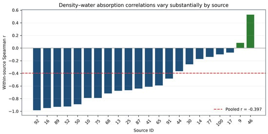
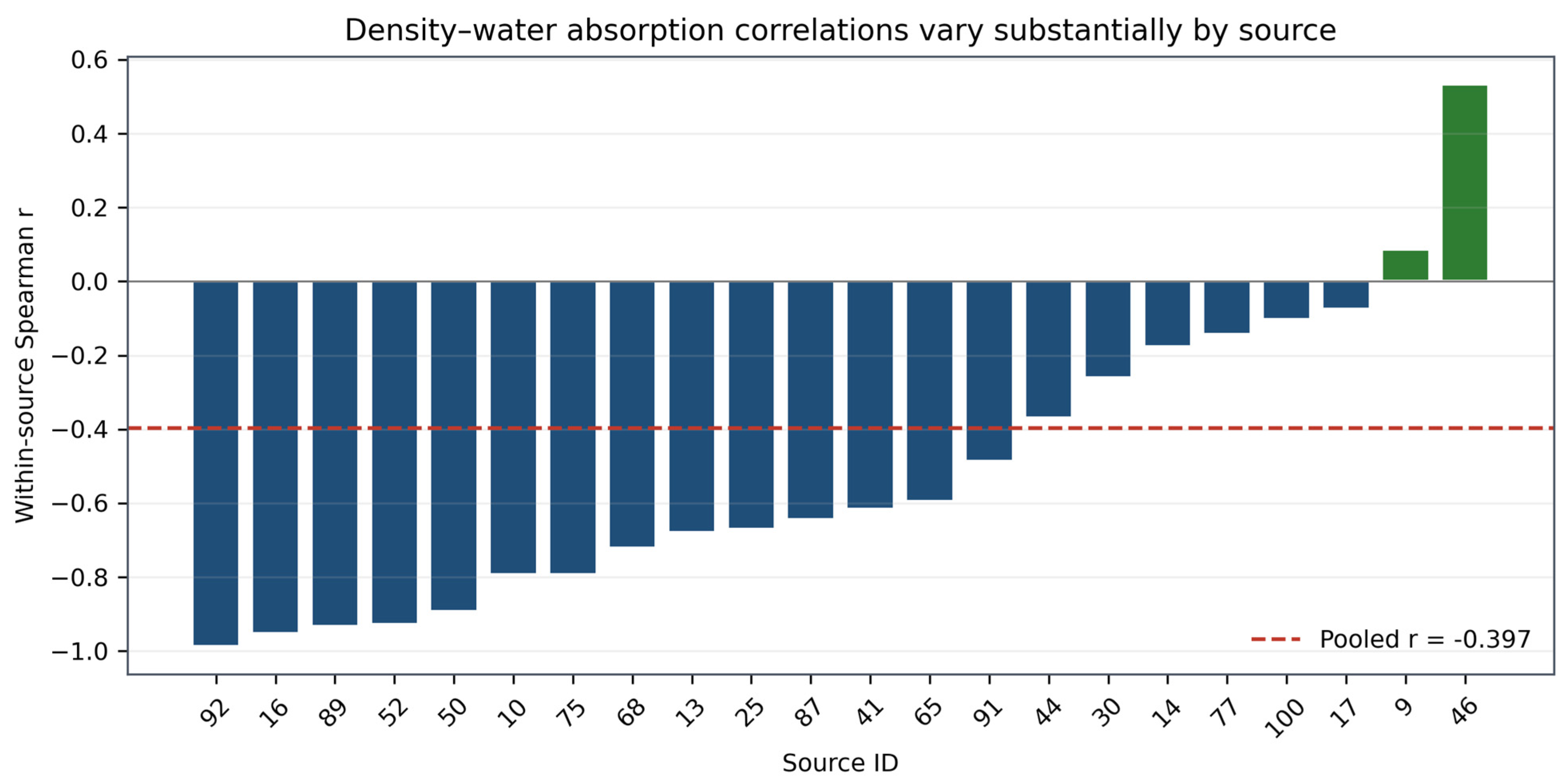
Pooled Spearman correlation between particle density and water absorption was r = −0.397 (N = 631; 95% bootstrap CI: [−0.459, −0.329]). There were 24 sources, of which at least five pairs of observations were observed. Twenty-two sources provided finite within-source correlation values, while Sources 2 and 3 provided undefined correlation values due to one of the variables being constant. Finite correlations varied between −0.987 and +0.533; 14 out of them had |r| > 0.5, and two were positive, see Table 6. The sign change along with high variation between sources indicates Simpson-like heterogeneity. Despite a negative pooled correlation (r = −0.397), within-source correlations vary from −0.987 to +0.533. Based on bootstrap 95% confidence intervals for 22 finite correlations (Table 7), it can be seen that 12 out of 22 have confidence intervals that do not include zero. However, the two positive correlations (Source 9: r = 0.086, p = 0.832; Source 46: r = 0.533, p = 0.210) have confidence intervals that do include zero. This shows that these particular reversals are statistically insignificant and most likely a result of small sample sizes.

Table 6. Within-source density–water absorption correlations for sources with at least five paired observations.

Source ID	N	Within-Source Spearman r
2	12	NA (constant variable)
3	20	NA (constant variable)
9	6	+0.086
10	14	−0.793
13	7	−0.679
14	16	−0.176
16	8	−0.952
17	24	−0.075
25	120	−0.670
30	24	−0.261
41	36	−0.616
44	10	−0.370
46	9	+0.533
50	7	−0.893
52	102	−0.928
65	15	−0.595
68	12	−0.720
75	26	−0.792
77	29	−0.142
87	23	−0.644
89	9	−0.933
91	6	−0.486
92	24	−0.987
100	35	−0.103

Table 7. Bootstrap 95% confidence intervals for within-source Spearman correlations (density vs. water absorption).

Source ID	N	r_Within	CI_Low	CI_High	p_Approx
2	12	NA	NA	NA	NA
3	20	NA	NA	NA	NA
9	6	+0.086	−1.000	+1.000	0.832
10	14	−0.793	−1.000	−0.234	0.010
13	7	−0.679	−1.000	+0.176	0.156
14	16	−0.176	−0.675	+0.406	0.548
16	8	−0.952	−1.000	−0.615	0.004
17	24	−0.075	−0.435	+0.253	0.638
25	120	−0.670	−0.751	−0.567	0.000
30	24	−0.261	−0.662	+0.219	0.264
41	36	−0.616	−0.815	−0.346	0.000
44	10	−0.370	−0.875	+0.465	0.316
46	9	+0.533	−0.368	+0.930	0.210
50	7	−0.893	−1.000	−0.348	0.014
52	102	−0.928	−0.978	−0.845	0.000
65	15	−0.595	−0.869	−0.019	0.042
68	12	−0.720	−0.957	−0.196	0.014
75	26	−0.792	−0.918	−0.523	0.000
77	29	−0.142	−0.552	+0.324	0.500
87	23	−0.644	−0.832	−0.311	0.002
89	9	−0.933	−1.000	−0.584	0.004
91	6	−0.486	−1.000	+0.939	0.398
92	24	−0.987	−0.999	−0.946	0.000
100	35	−0.103	−0.410	+0.246	0.488

Note: Sources 2 and 3 yielded undefined correlations (NA) because one of the variables was constant. The p_approx column represents the two-sided bootstrap p-value testing the null hypothesis of zero correlation.

In Figure 1 below, the within-source correlations and the overall correlation are compared, while Table 6 gives information about the two undefined constant-variable situations.

Figure 1. Within-source Spearman correlations between particle density-water absorption; the dashed line is the pooled correlation. Blue bars represent negative within-source correlations, green bars represent positive within-source correlations, and the red dashed line represents the pooled correlation (r = −0.397).

3.3. Source Effect on Density (ANOVA)

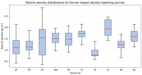
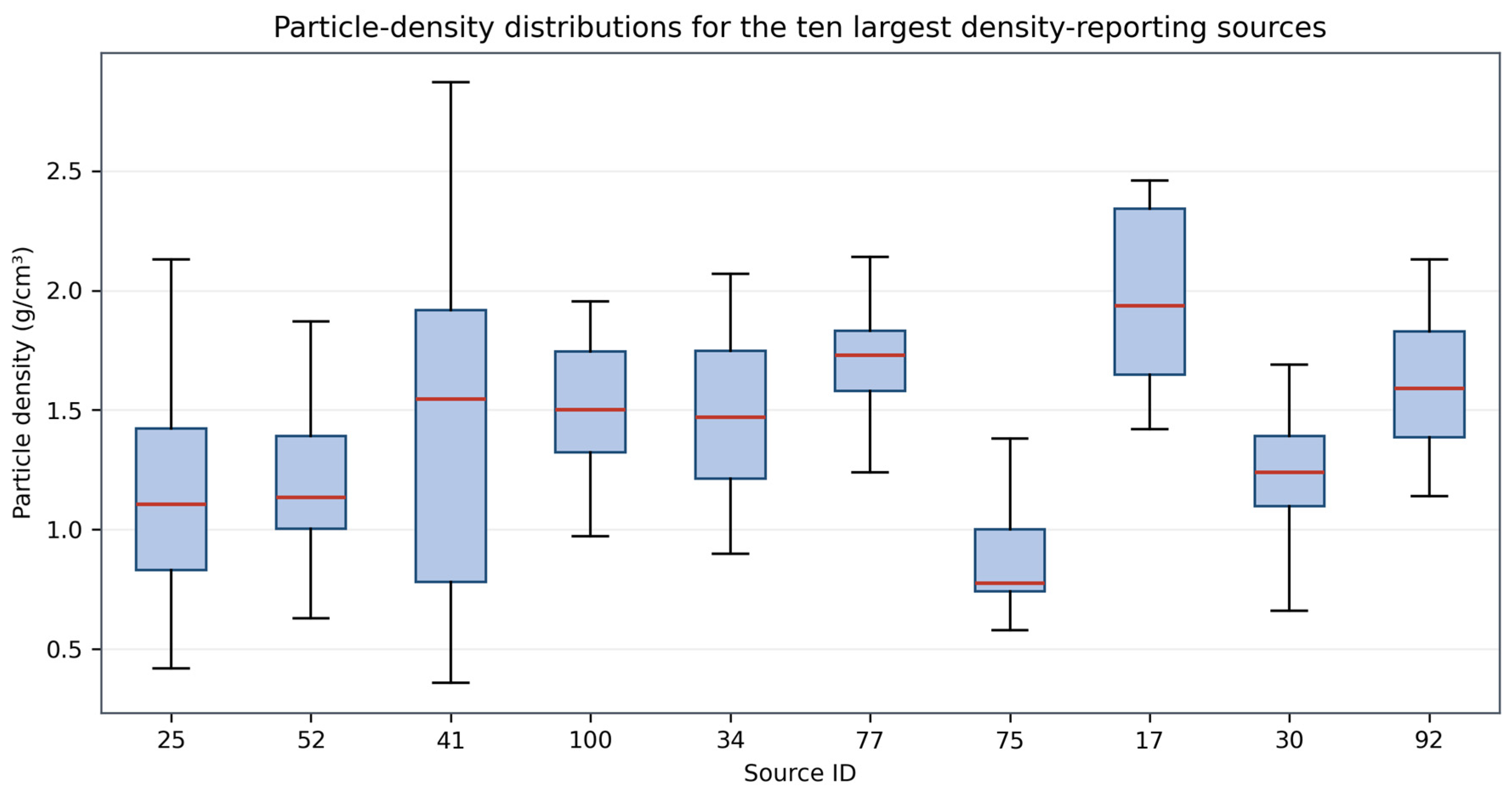
One-way analysis of variance conducted on the 693 density measures among 50 contributors produced F (49, 643) = 12.95, p < 0.001, with an η² of 0.497. Hence, 49.7% of the variance of density measurements was attributable to the sources. The one-way random effects intra-class correlation coefficient was 0.463 (with arithmetic mean size of groups) and 0.812 (with harmonic mean size of groups). Corrected sums of squares and mean squares can be seen in Table 8, while the top ten density sources are depicted in Figure 2.

Table 8. Corrected one-way ANOVA for particle density by source (N = 693; 50 sources).

Source	SS	Df	MS	F	p	η2
Between sources	88.205	49	1.800	12.95	<0.001	0.497
Within sources	89.367	643	0.139	—	—	—
Total	177.572	692	—	—	—	—

Note: One-way random-effects ICC(1) = 0.463 (calculated using arithmetic mean group size, k = 13.86) and 0.812 (calculated using harmonic mean group size, k = 2.77). The harmonic mean is reported to transparently account for the unbalanced number of observations across sources.

Figure 2. Particle-density distributions for the ten largest density-reporting sources. Blue bars are used to illustrate the interquartile range (IQR), the red lines represent the median, while the whiskers are extended till the furthest outlying value.

3.4. Source-Level Descriptive Synthesis Results

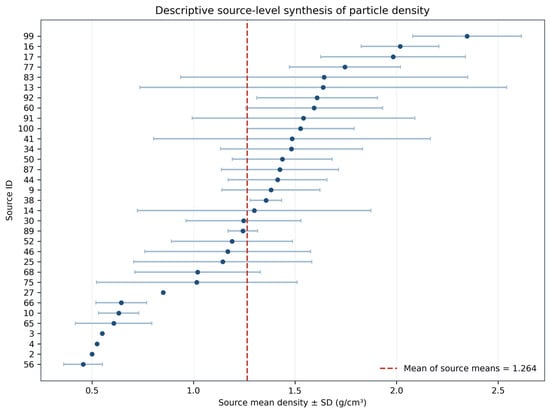
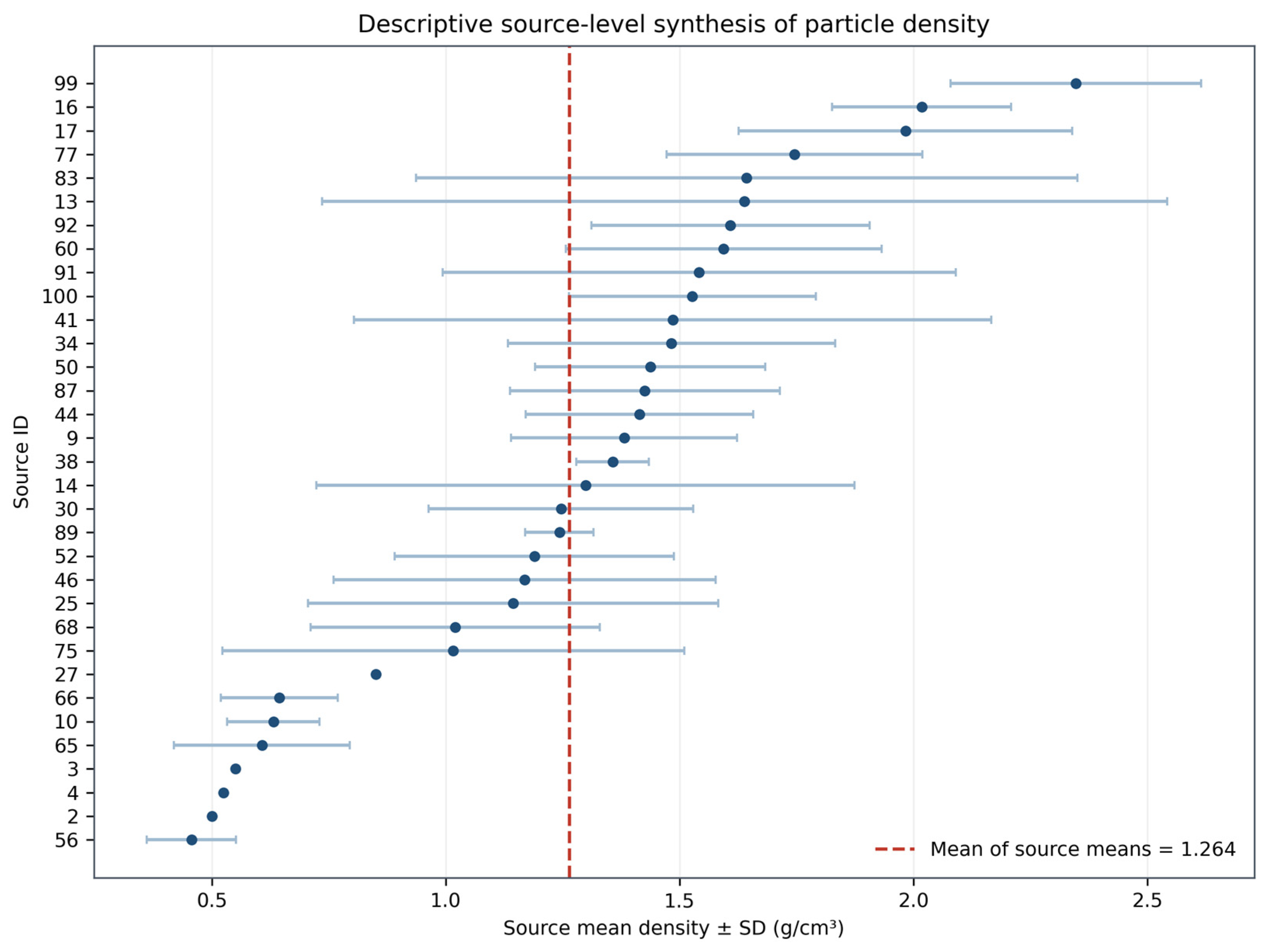
Of the 33 sources having at least three density estimates, the equally weighted average of the means was 1.264 g/cm³, and the median was 1.357 g/cm³; the range of the source means was 0.456–2.348 g/cm³. Figure 3 shows the source means and within-source standard deviations. A meta-analytic mean by inverse variance weighting was not provided since some sources had zero within-source variance, and there was no estimation of a common treatment effect in the experiments.

Figure 3. Descriptive source-level particle-density means ± SD for sources with at least three measurements.

Source density distributions are presented in graphical form in Figure 3.

Source summary details, such as source ID, number of observations, and particle density mean ± standard deviation, are presented in Table S1 (Supplementary Materials).

3.5. Cross-Source Generalization Failure (LOSO)

Table 9 outlines the LOSO process for selecting sources. Out of 78 sources, 19 had all the necessary cases for the three-predictor production model (Clay, Temp, Time, and Density). Of those, nine sources passed the evaluation criteria (≥3 test observations and ≥20 training observations), while one source (Source 27) was discarded because of the constant outcome variance (R² was undefined).

Table 9. LOSO source selection log showing the eligibility of the 19 sources with complete data for the 3-predictor model.

Source ID	N Test	N_Train	SD_Test	Status
7	2	276	0.127	excluded (<3 test obs)
9	6	272	0.242	eligible
12	2	276	0.205	excluded (<3 test obs)
14	16	262	0.575	eligible
16	8	270	0.192	eligible
17	24	254	0.357	eligible
20	2	276	0.255	excluded (<3 test obs
24	2	276	0.075	excluded (<3 test obs)
27	4	274	0.000	R2 undefined (constant)
30	24	254	0.283	eligible
32	1	277	0.000	excluded (<3 test obs)
33	1	277	0.000	excluded (<3 test obs)
34	34	244	0.350	eligible
41	36	242	0.681	eligible
42	2	276	0.310	excluded (<3 test obs)
44	10	268	0.243	eligible
52	102	176	0.299	eligible
84	1	277	0.000	excluded (<3 test obs)
86	1	277	0.000	excluded (<3 test obs)

Note: Out of the 78 sources, only 19 had complete cases for the 3-predictor model (Clay, Temp, and Time). Nine sources met the threshold for evaluation, and one (Source 27) was excluded due to constant outcome variance.

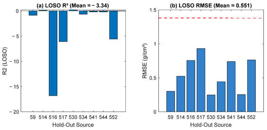
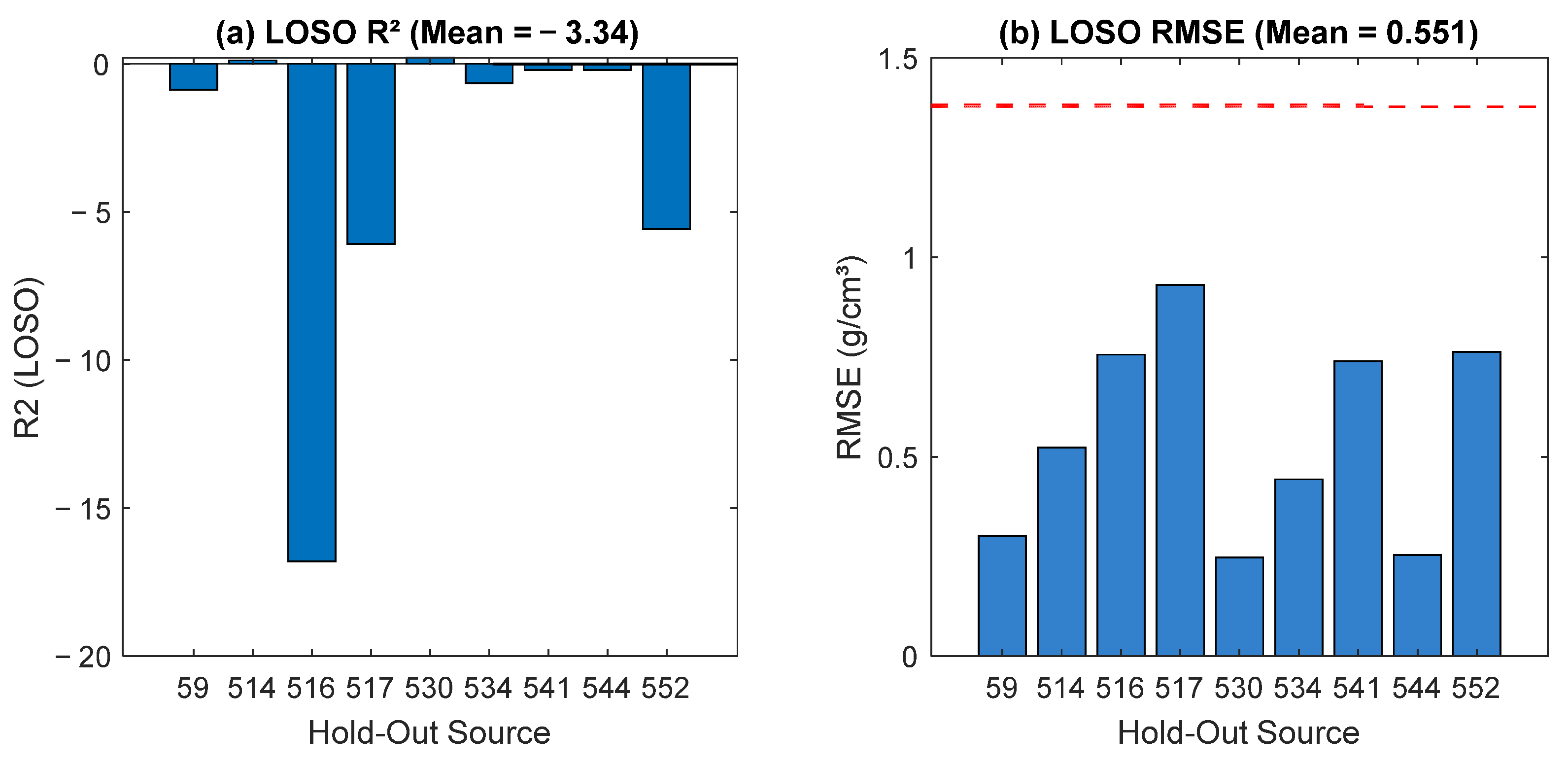
A Random Forest was trained on the data and tested on each of nine sources. Detailed results are shown in Table 10. The Random Forest model produced a mean R² of −3.345 (median −0.654). A total of two out of nine sources had a positive R². More importantly, when comparing it to a naïve baseline model (training mean predictor), the Random Forest performed worse in seven out of nine sources, with the naïve mean R² being −2.096. Figure 4 clearly demonstrates the inability of the model to perform. In conclusion, the production model fails to predict novel sources’ properties.

Table 10. Leave-one-source-out cross-validation results for the complete-case production model.

Source ID	N Test	R2_RF	MAE_RF	RMSE_RF	R2_Naive	MAE_Naive
9	6	−0.875	0.216	0.302	−0.002	0.191
14	16	+0.119	0.445	0.523	−0.019	0.476
16	8	−16.805	0.733	0.756	−13.777	0.665
17	24	−6.090	0.826	0.930	−3.674	0.669
30	24	+0.207	0.191	0.247	−0.244	0.248
34	34	−0.654	0.354	0.443	−0.135	0.303
41	36	−0.211	0.642	0.739	−0.038	0.574
44	10	−0.209	0.211	0.254	−0.037	0.198
52	102	−5.587	0.643	0.763	−0.935	0.351

Note that the Random Forest underperformed the naïve baseline (predicting the training mean) in 7 out of 9 sources, indicating a failure to capture transferable signals.

Figure 4. Leave-one-source-out cross-validation analysis for complete-case production model: (a) R² statistics for the held-out source; where green bars denoted positive R² and blue bars denote negative R²; (b) RMSE values for each held-out source (blue bars); with the red dashed line represents naive baseline RMSE.

Table 11 Leave-one-source-out cross-validation after fold-safe KNN imputation (k = 5); imputation resulted in an increase in the number of evaluable sources to 29 but a decrease in the mean R² to −7.634 (median −1.107).

Table 11. LOSO cross-validation results after fold-safe KNN imputation (k = 5).

Source ID	N Test	R2	MAE	RMSE
9	6	−0.410	0.172	0.262
10	14	−6.741	0.238	0.265
3	7	−0.284	0.746	0.948
14	16	0.165	0.443	0.509
16	8	−22.438	0.815	0.868
17	24	−6.365	0.820	0.948
25	120	0.016	0.356	0.433
30	24	−1.022	0.298	0.394
34	34	−0.214	0.307	0.379
38	6	−0.146	0.066	0.076
41	36	−0.019	0.583	0.678
44	10	−0.180	0.206	0.251
46	9	0.199	0.315	0.345
50	7	−1.107	0.287	0.331
52	102	−6.490	0.690	0.813
56	5	−55.989	0.639	0.645
60	5	−1.587	0.476	0.486
65	15	−21.354	0.819	0.861
66	12	−23.982	0.585	0.598
68	12	−1.676	0.461	0.485
75	26	0.035	0.299	0.476
77	29	−2.492	0.452	0.502
83	3	−0.003	0.455	0.579
87	23	−1.249	0.342	0.424
89	9	−12.972	0.247	0.257
91	6	0.353	0.298	0.403
92	24	−0.481	0.279	0.354
99	4	−52.595	1.684	1.700
100	35	−2.346	0.429	0.476

Note: Compared to the complete-case LOSO (Table 10), fold-safe imputation expanded the evaluable sources to 29 but drastically reduced the mean R² to −7.634 (median −1.107). This confirms that imputation introduces artifacts that artificially inflate random-fold performance (Section 3.1) but fail to restore cross-source transferability.

In an exploratory robustness analysis, the 19 sources with no missing values were clustered into three groups based on their standardized source-level production means. While all three hold-out groups yielded negative R² values (Table 12), one of them had only three observations. LOCO thus corroborates the LOSO result in terms of the sign but shows the instability of the clustered estimates with limited coverage.

Table 12. Exploratory three-cluster leave-one-cluster-out validation.

Cluster	N Sources	N Test	R2
1	2	3	−78.602
2	14	148	−0.226
3	3	127	−0.802

LOCO is viewed as a sensitivity analysis exercise rather than an attempt to replace source validation.

3.6. Waste Materials

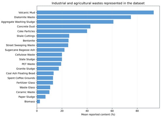
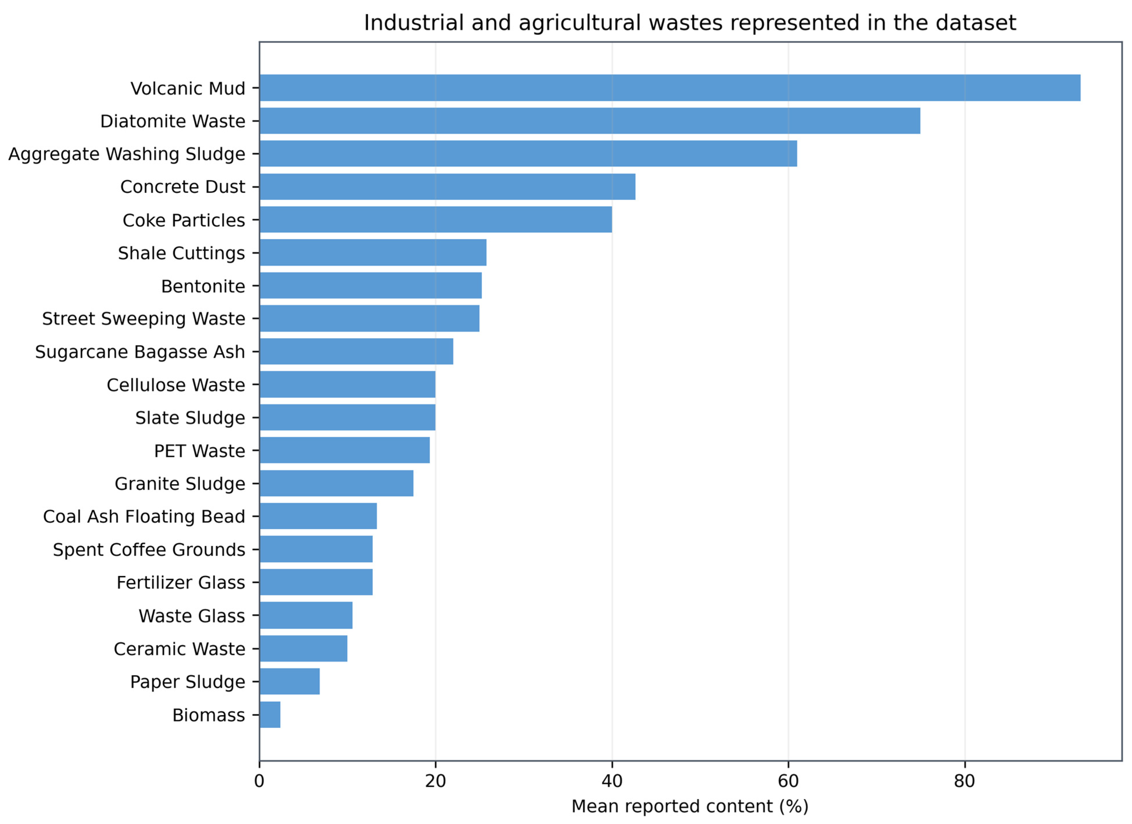
Twenty different types of waste are presented systematically in Table 13 and Figure 5. The three wastes having the highest average contents are volcanic mud (93.1%, N = 35), diatomite waste (75.0%, N = 24), and aggregate washing sludge (61.0%, N = 26).

Table 13. Industrial and agricultural waste utilization in LWA production.

Waste Category	N	Mean Content (%)
Volcanic_Mud	35	93.14
Diatomite_Waste	24	75.00
Bentonite	3	67.33
Aggregate_Washing_Sludge	26	61.00
Coke_Particles	2	60.00
Slate_Sludge	10	52.00
Granite_Sludge	10	45.50
Sugarcane_Bagasse_Ash	12	44.00
Concrete_Dust	6	42.67
Shale_Cuttings	5	41.20
Fertilizer_Glass	3	30.00
Street_Sweeping_Waste	3	25.00
Cellulose_Waste	9	20.00
Paper_Sludge	12	20.00
PET_Waste	6	19.33
Spent_Coffee_Grounds	6	15.00
Coal_Ash_Floating_Bead	3	13.33
Waste_Glass	8	11.88
Ceramic_Waste	1	10.00
Biomass	1	4.80

Figure 5. Mean reported content of the waste materials represented in the dataset.

Model-Agnostic Robustness Check

In order to test the robustness of our complete-case analysis to Random Forest, we applied Strategy A using Gradient Boosting and RBF-kernel SVR (see Table 14).

Table 14. Algorithmic robustness check for Strategy A.

Algorithm	Mean 5-Fold R2 ± SD	Mean RMSE
Random Forest	0.158 ± 0.096	0.473
Gradient Boosting	−0.001 ± 0.141	0.462
SVR (RBF)	0.089 ± 0.265	0.437

Random Forest and Gradient Boosting gave mean R² close to or below zero, but for SVR, mean R² was equal to 0.089. None of the production-only methods performed well in predicting random folds for complete cases.

3.7. Modeling Strategies: Baseline vs. Feature Engineering

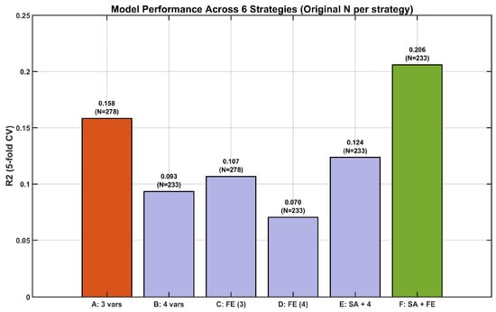
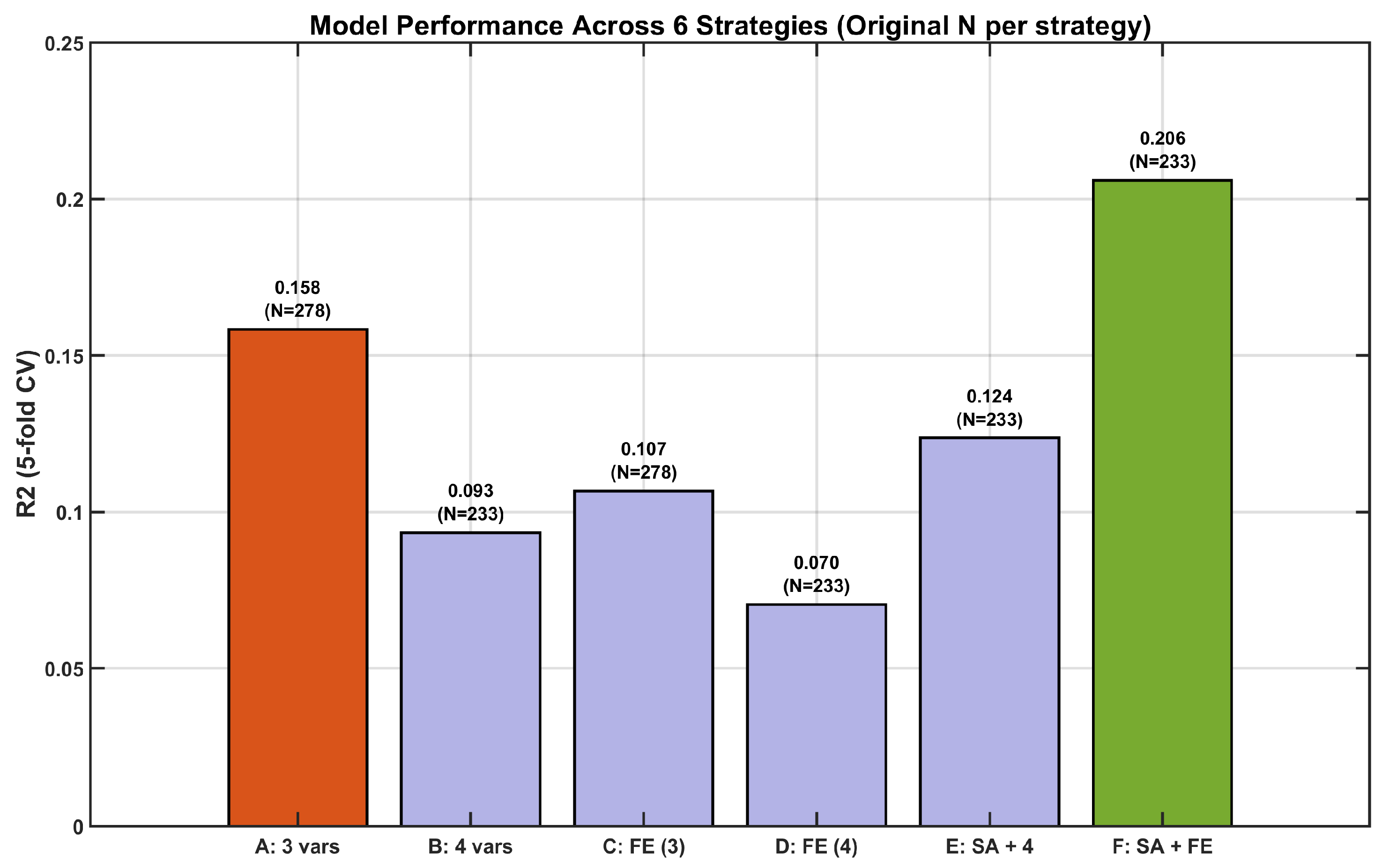
Strategies A-F are compared in Table 15 and Figure 6. Modeling Strategies A-D rely only on production data; Strategies E and F also employ source variables and thus assess within-source interpolation and not unseen-source prediction.

Table 15. Five-fold cross-validated performance of the six modeling strategies.

Strategy	N	Mean R2	SD	RMSE
A: 3 vars	278	0.158	0.079	0.427
B: 4 vars	233	0.093	0.119	0.453
C: FE (3)	278	0.107	0.123	0.439
D: FE (4)	233	0.070	0.153	0.458
E: SA + 4	233	0.124	0.117	0.368
F: SA + FE	233	0.206	0.175	0.350

Figure 6. Mean 5-fold R² (±SD) for six modeling strategies. Strategies E–F include source indicators and quantify within-source interpolation.

Observation 1: The provision of waste data failed to enhance the production model. In the initial test (Table 15), the R² value for Strategy A was 0.158 compared to 0.093 for Strategy B. In order to determine whether the decline was simply due to the decline in the sample size, an N-unified comparison was conducted (Table 16). With an identical sample size (N = 233), Strategy A (R² = 0.132) continued to perform better than Strategy B (R² = 0.093).

Table 16. N-unified fair comparison of the six modeling strategies (N = 233 complete cases).

Strategy	N_Unified	R2_Mean	R2_Std	RMSE
A: 3 vars	233	0.132	0.101	0.443
B: 4 vars	233	0.093	0.119	0.453
C: FE (3)	233	0.073	0.156	0.457
D: FE (4)	233	0.070	0.153	0.458
E: SA + 4	233	0.124	0.117	0.368
F: SA + FE	233	0.206	0.175	0.350

Note: By holding the sample size constant at N = 233, the comparison isolates the effect of the features. Strategy A (3 variables) achieved an R² of 0.132, while Strategy B (+Waste) achieved 0.093 (ΔR² = −0.038). This confirms that a large part of the apparent deterioration in Table 15 was driven by the reduction in sample size, though waste content still does not add predictive value.

Observation 2: The addition of artificially generated nonlinear and interaction terms (Strategies C and D) did not improve the out-of-fold results relative to the respective base strategies (A and B), again underscoring the constraints imposed by data coverage.

Observation 3: The use of source-specific features (Strategies E and F) increased the average random-fold R² to 0.206 (Strategy F). This implies that the ML algorithm can classify sources and extrapolate for known sources, but this is not the same as predicting across sources.

Observation 4: The ML models were able to achieve a random-fold R² of 0.206 (Strategy F), which represents an improvement over the simple base strategy of taking a global mean (R² = −0.014) and linear regression (R² = −0.011) demonstrated in Section 3.8. But any such benefit disappears completely in out-of-source validation, where the ML models underperform the naïve baseline (Table 10).

Model (5), the random intercepts mixed effects model, converged on N = 278 cases across 19 sources. The source variance was 0.225, while the residual variance was 0.143 with an ICC of 0.612 (Table 17).

Table 17. Random-intercept mixed-effects model with standardized fixed effects (N = 278; 19 sources).

Term or Component	Estimate	p-Value or Share
Intercept (β)	1.282	<0.001
Clay, standardized (β)	0.180	<0.001
Temperature, standardized (β)	0.022	0.507
Time, standardized (β)	−0.048	0.315
Source random-intercept variance	0.225	61.2% of total
Residual variance	0.143	38.8% of total

Taking into account source clustering, standardized clay was positively related to density (β = 0.180, p < 0.001), while sintering temperature (β = 0.022, p = 0.507) and sintering time (β = −0.048, p = 0.315) were not significantly correlated. These are source-adjusted associations, not causal effects.

3.8. Out-of-Fold Permutation Feature Importance Results

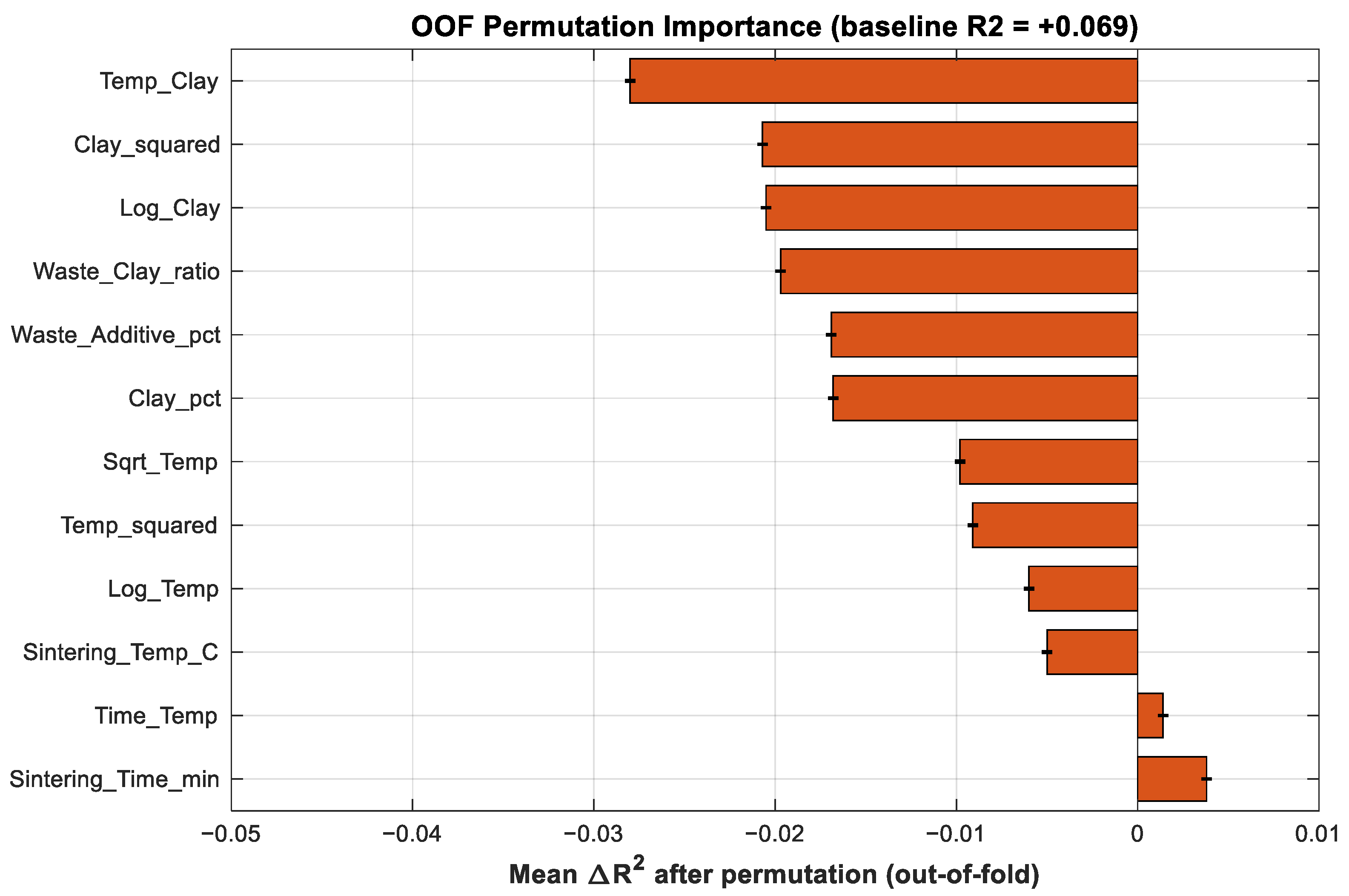
In Table 18, the comparison of the ensemble ML models is made with two baseline models: global mean and linear regression (clay, temperature, time). Both baseline models produced nearly zero values for the coefficient of determination (R² = −0.014 and −0.011, respectively), which shows that small improvements achieved by the ML models in the random folds were not repeated in the LOSO. Permutation importance of Strategy D is shown in Table 19 and Figure 7. The out-of-fold baseline R² of the model is 0.069. The mean change in R² (ΔR²) for all the features is less than 0.01, and the standard deviation exceeds the mean. This suggests that none of the artificial or natural features contributes to prediction in an out-of-fold fashion. What needs to be noted here is that this does not mean that these production features lack any physical meaning but that in the context of the examined model and dataset they provide no consistent predictive signal.

Table 18. Baseline models performance for comparison against machine learning algorithms.

Model	R2_Mean	RMSE_Mean
lobal_mean	−0.014	0.470
Linear_ClayTempTime	−0.011	0.469

Note: Both the global mean and standard linear regression yield R² values near zero. While the ensemble ML models achieve slightly higher R² in random 5-fold cross-validation (e.g., Strategy F = 0.206), they fail to a significantly greater extent than these baselines in the LOSO setting. This underscores that the apparent ML performance is an artifact of random partitioning, not true cross-source transferability; see Table 19.

Table 19. Out-of-fold permutation importance for Strategy D (30 permutations per fold).

Order	Feature	Mean ΔR2 After Permutation	SD
1	Sintering_Time_min	0.0038	0.0047
2	Time_Temp	0.0014	0.0082
3	Sintering_Temp_C	−0.0050	0.0115
4	Log_Temp	−0.0060	0.0135
5	Temp_squared	−0.0091	0.0119
6	Sqrt_Temp	−0.0098	0.0147
7	Clay_pct	−0.0168	0.0062
8	Waste_Additive_pct	−0.0169	0.0070
9	Waste_Clay_ratio	−0.0197	0.0060
10	Log_Clay	−0.0205	0.0060
11	Clay_squared	−0.0207	0.0062
12	Temp_Clay	−0.0280	0.0120

Note: The baseline out-of-fold R² for this model was 0.069. All features yielded a mean reduction in R² (ΔR²) of less than 0.01, with standard deviations exceeding the mean. This indicates that none of the variables provided a consistent out-of-fold predictive contribution. However, this does not imply that these production variables lack physical relevance; rather, it highlights their lack of stable predictive signal within the evaluated model and data coverage.

Figure 7. Out-of-fold permutation importance for Strategy D. Negative means indicate no stable predictive contribution.

As a result, the previous rank of the engineered variables was dropped since it is not significant given that all the permutation effects out-of-fold are non-positive.

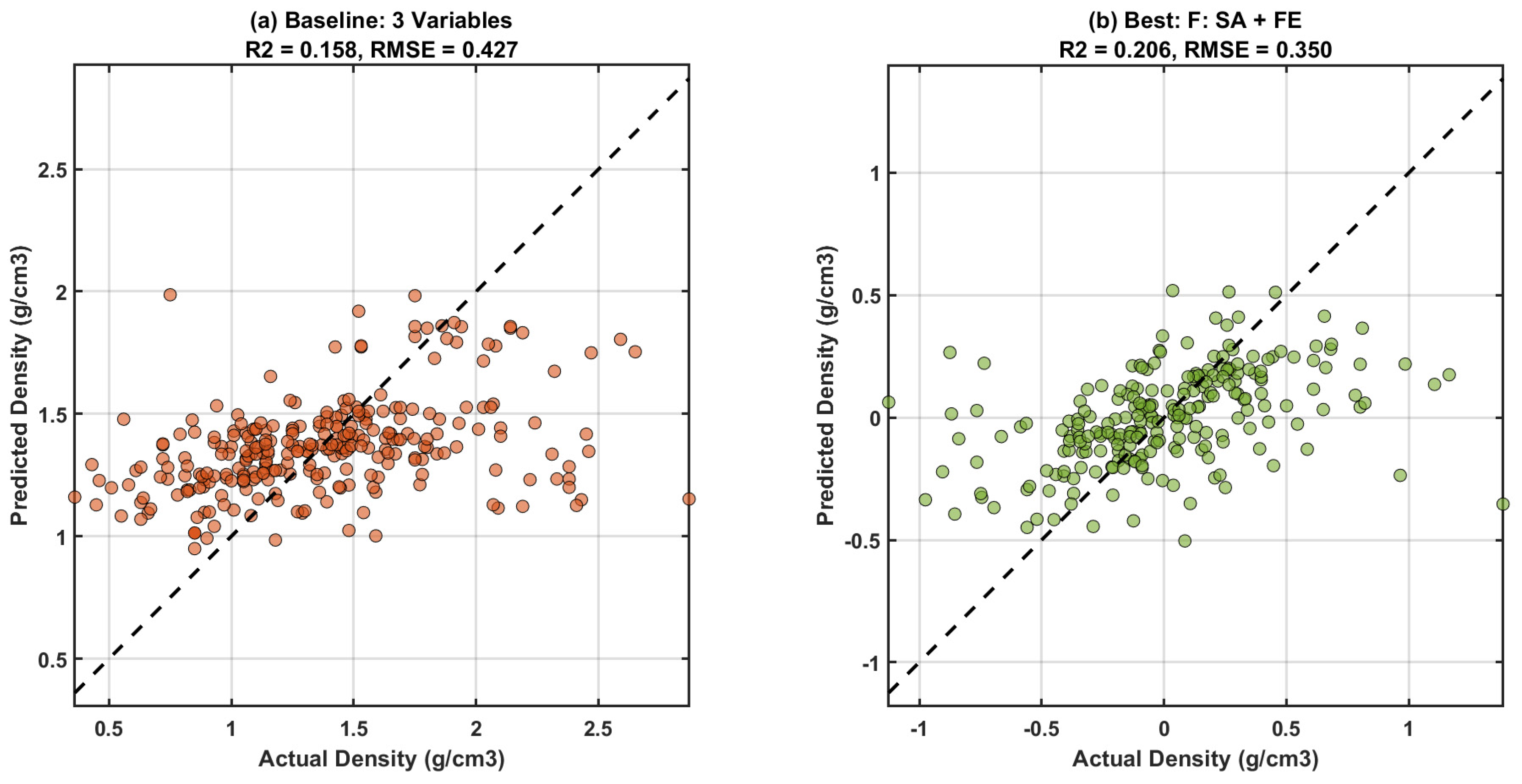
Figure 8 shows the results of the out-of-fold predictions. Strategy A gave an out-of-fold R² value of 0.158 on the original density scale. The use of source-specific features (Strategy F) boosted the out-of-fold R² value up to 0.206 on the original (uncentered) density scale. For illustrative purposes, Figure 8b plots the Strategy F out-of-fold predictions on the source-centered density scale (which is why there are negative values); however, the R² and RMSE values presented were computed with the addition of the source means from the training folds, that is, on the original non-centered scale. This demonstrates the capability of source-specific features for better interpolation among known sources, but it is obvious from the LOSO results that this cannot solve the problem of predicting novel sources.

Figure 8. Prediction versus actual density for (a) Strategy A using original density scale and (b) Strategy F using source-centered scale. Source centering helps with within-source interpolation but cannot account for unseen sources.

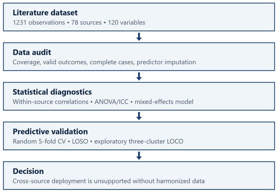
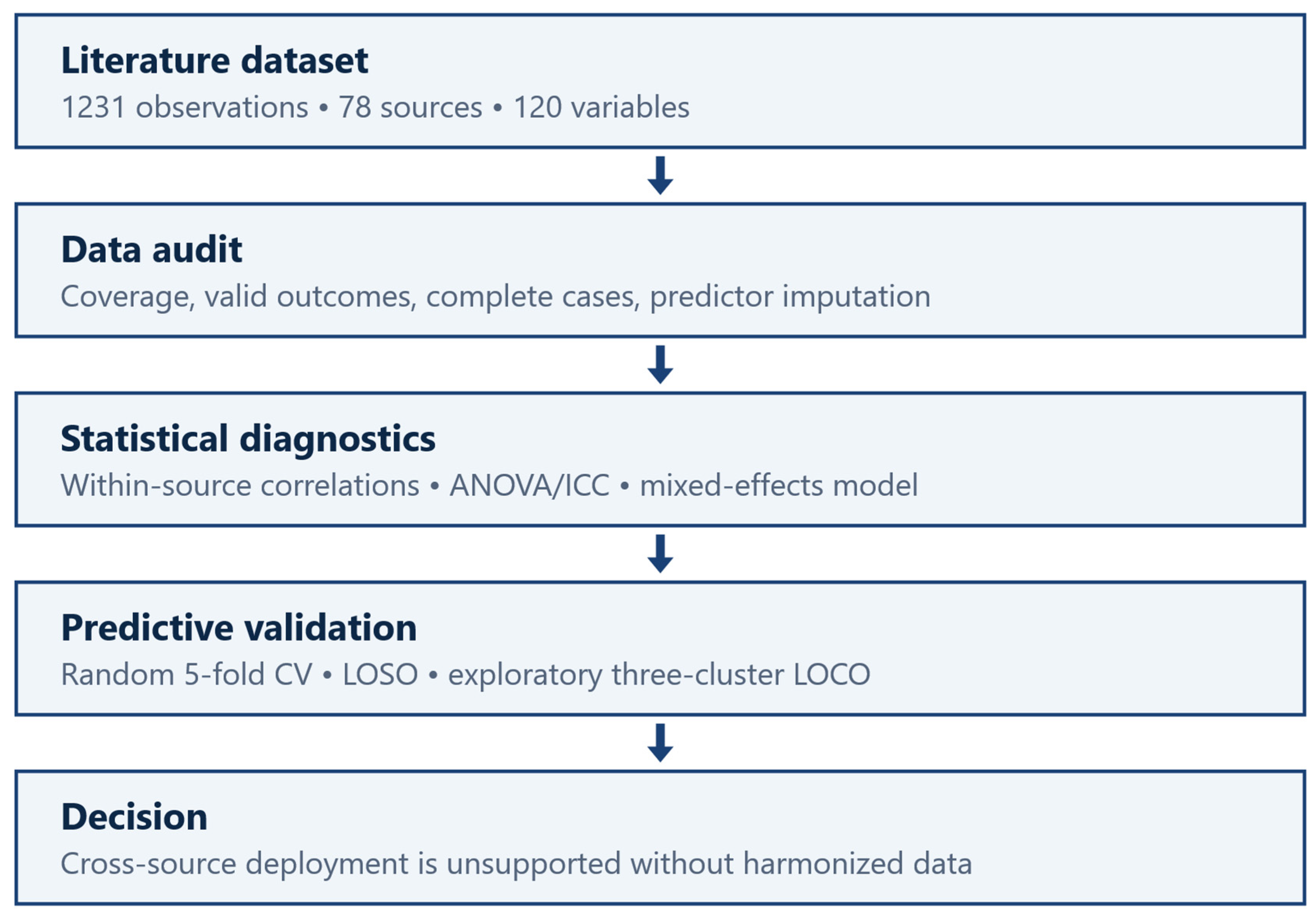
The audited process flow can be seen in Figure 9, which includes literature extraction, coverage/missing checks, diagnostics, random-fold modeling, unseen source validation, and finally the decision to deploy. The main complete-case analysis is coupled with predictor imputation sensitivity analysis, but outcome imputation never occurred.

Figure 9. Audited methodology workflow from literature extraction through cross-source deployment assessment.

4. Discussion

4.1. Why Simpson-like Aggregation Effects Matter for Materials Informatics

The relationship between density and absorption differs across various sources (Figure 1, Table 6). In fact, while 20 out of 22 finite sources have the same negative direction for the estimated pooled relationship, two exhibited positive correlations, although non-significant (Source 9: r = 0.086, p = 0.832; Source 46: r = 0.533, p = 0.210). Nevertheless, both of these positively correlated results are fairly low in their values and insignificant, which is proven by their bootstrap confidence intervals including zero and 14 have |r| > 0.5. Although this is not a pure instance of Simpson’s paradox since most strata do not reverse signs, the behavior is certainly in line with a Simpson-like aggregation effect. The consequence for application here is that the pooled correlation cannot be directly applied to individual sources without source-specific validation. Furthermore, a lack of reversal in sign does not mean that there is homogeneity; heterogeneity in magnitude alone renders the common-slope assumption for pooling invalid.

4.2. Why Source Identity Dominates

The revised ANOVA model reveals that 49.7% of the total variation in particle density is explained by the clustering among the 50 sources (Table 8). Both the one-way (0.463) arithmetic and (0.812) harmonic and adjusted mixed-effects ICC (0.612) confirm significant clustering. The random fold approach can take advantage of this when source variables are available, However, LOSO actually investigates whether the production factors can be applied to unknown sources.

4.3. Why Feature Engineering Is Limited by Data Coverage

Absence of predictors had a considerable impact on the number of cases and performance using random folds: fold-safe imputation expanded the number of cases to 693 up from 278 and improved the mean R² to 0.247 to 0.271. Yet out-of-source leave-one-source-out performance stayed negative, and engineered predictors did not have any stable out-of-fold permutation importance. Better reporting enhances the model fitting but does not alone eliminate source heterogeneity.

4.4. Physical and Technological Mechanisms for Heterogeneity of Source Data

While the association statistic effect detected in the presented research (η² = 0.497) does not specify any physical mechanisms on its own, there are a number of physical and technological features known for LWA manufacturing that may account for the noted variance.

First of all, the composition of raw materials differs considerably: the clay component in our dataset varies between 0% and 100% and includes a variety of mineral types (such as illite, kaolinite, montmorillonite) having different melting points and bloating capacity. Second, sintering conditions define the vitrification level and the porosity structure: in our sample, the sintering temperature varies between 700 °C and 1350 °C, while the time range is between 0 and 360 min. Third, fluxes and bloating components (Na₂O, K₂O, Fe₂O₃, and carbon) have a dominant effect on the density, although they are reported inconsistently. Fourth, the measurement procedure may differ in different laboratories (pycnometry, geometric method, and Archimedes’ principle). It is the differences in their methodology that make it impossible for the model to be generalized to other sources’ protocols, further emphasizing the necessity of source-aware diagnosis suggested in this framework.

4.5. Comparison with Prior Literature

Large values of R² reported in previous LWA ML studies [12,13,14] usually correspond to within-source predictions using random partitioning or small experimental ranges. However, this is a different case from prediction of a new literature source. In the current dataset, source characteristics contributed to achieving R² ≈ 0.206 by random-fold interpolation, while production-only LOPO was weak. The performance claims should also describe the population for which the test was intended to be used.

4.6. Recommendations for the Materials-Informatics Community

R1. Measure source heterogeneity prior to modeling. Utilize the CSGD approach (Section 2.4.8) to assess whether pooling of data justifies the target predictive problem.

R2. Use the leave-one-source-out validation approach if claiming deployment to unseen sources (Figure 4, Table 10). Consider cluster-based validation to be exploratory in case clusters are small (Section 3.5).

R3. Present both pooled and within-source relationships (Figure 1, Table 6). Employ mixed effects models to measure source-adjusted associations, but avoid causal wording in the absence of causal design (Section 3.7).

R4. Describe data availability and numbers of observed outcomes for all models (Table 1 and Table 5). Train imputers inside training folds, not using imputed outcomes as observed data.

R5. Use imputation as an open sensitivity analysis but not as the proof of cross-source validity. Compare random fold imputation results with unseen-source validation (Section 3.1 and Section 3.5).

4.7. Limitations

There are several issues that need to be considered. First, there were just 278 observations available with complete data for the four predictors. Second, imputation of predictors increases the number of random folds in the sample but does not account for unreported experimental conditions. Third, the LOSO prediction is based on nine non-constant held-out sources, while the LOCO exploratory analysis considers one extremely small cluster. Fourth, the source variables measure the extent of interpolation among the known sources and cannot be obtained for an unknown source. Fifth, mixed-effects predictions are purely associational. Sixth, some important predictors have not been reported.

5. Conclusions

• In the analysis of 1231 LWA experiments from 78 different sources, the following five findings were observed to be related to each other:
  There is significant heterogeneity of the aggregated density absorption relationship, which consists of sign reversals for some of the sources (two out of 22), and magnitude variations ranging from −0.987 to +0.533. Such a finding indicates that there is Simpson-like effect on aggregation (the aggregated coefficient does not reflect variability of the coefficient across sources) and does not correspond to Simpson’s paradox (Figure 1, Table 7).
• The source variable explains 49.7% of the density variation (η² = 0.497, p < 0.001). One-way ICC was calculated to be 0.463 (arithmetic mean) and 0.812 (harmonic mean) (Table 8).
• Production feature models are not sufficient to generalize for new data sources as LOSO produced a mean R² = −3.345 for nine tested sources, which is even lower than a naïve prediction based on the training average (see Table 10).
• Fold-safe predictor imputation increased the sample size and improved random-fold predictions (R² = 0.247–0.271) but negatively impacted cross-source generalization, reducing LOSO R² to −7.634 (see Table 11; −4.108 when restricted to the same nine sources). Thus, predictor imputation cannot recover generalizability to new unseen data sources.
• Source-specific predictors (Strategy F) generated the highest within-source random-fold predictions (R² = 0.206), whereas engineered production predictors provided no consistent predictor importance out-of-fold (Table 19). Hence, validation strategies should reflect the intended usage environment.

Scope and Limitations of the Study

Conclusions from this study are strictly limited to the scope of the investigated database (1231 experiments from 78 sources), the chosen input parameters (clay, temperature, time, and waste percentage), and the utilized machine learning models (ensemble tree-based models). The absence of cross-laboratory generalization does not mean that there is no possibility of developing a ML model for predicting across LWA databases. However, within the framework of current data gathering strategy, where such crucial parameters as heating rate (16.8%) and flux (1.9%) are rarely reported, cross-laboratory predictions were not substantiated by the current data and model methodologies. The CSGD framework suggested by the researchers should be considered as a diagnostic tool before using ML models rather than a predictive model per se.

These finding supports the need for the CSGD framework. Future work should estimate the source effect size, compare aggregated versus within-source dependencies, validate on novel sources, and conduct coverage audits before making claims about generalization.

References

- Andrew, R.M. Global CO2 emissions from cement production. Earth Syst. Sci. Data 2018, 10, 195–217. [Google Scholar] [CrossRef] [Scilit]
- Scrivener, K.L.; John, V.M.; Gartner, E.M. Eco-efficient cements: Potential economically viable solutions for a low-CO2 cement-based materials industry. Cem. Concr. Res. 2018, 114, 2–26. [Google Scholar] [CrossRef] [Scilit]
- Chandra, S.; Berntsson, L. Lightweight Aggregate Concrete: Science, Technology, and Applications; Noyes Publications: Norwich, NY, USA, 2002. [Google Scholar]
- Al-Hadithi, A.I.; Hilal, N.N.; Al-Gburi, M.; Midher, A.H. Structural behavior of reinforced lightweight self-compacting concrete beams using expanded polystyrene as coarse aggregate and containing polyethylene terephthalate fibers. Struct. Concr. 2023, 24, 5808–5826. [Google Scholar] [CrossRef] [Scilit]
- Cobo-Ceacero, C.J.; Cotes-Palomino, M.T.; Márquez-Montes, L.; Martínez-García, C.; Troyano-Pérez, F.J.; López, A.B. Contribution to environmental sustainability through artificial lightweight aggregates manufactured from waste. Clean Technol. 2026, 8, 95. [Google Scholar] [CrossRef] [Scilit]
- Li, Q.; Wang, B.; Yang, L.; Liu, C. Preparation and characteristics of cold-bonded lightweight aggregates by recycling mine tailings and industrial waste residues based-binder. J. Build. Eng. 2024, 95, 110190. [Google Scholar] [CrossRef] [Scilit]
- Riley, C.M. Relation of chemical properties to the bloating of clays. J. Am. Ceram. Soc. 1951, 34, 121–128. [Google Scholar] [CrossRef] [Scilit]
- Velis, C.A.; Franco-Salinas, C.; O’Sullivan, C.; Najorka, J.; Boccaccini, A.R.; Cheeseman, C.R. Up-cycling waste glass to minimal water adsorption/absorption lightweight aggregate by rapid low temperature sintering: Optimization by dual process-mixture response surface methodology. Environ. Sci. Technol. 2014, 48, 7527–7535. [Google Scholar] [CrossRef] [Scilit] [PubMed]
- Almajeed, E.A.; Turki, S.K. Synthesis of expanded clay aggregate pellets by using local raw materials. J. Univ. Babylon Eng. Sci. 2018, 26, 345–353. [Google Scholar] [CrossRef] [Scilit]
- Zhang, Y.; Aslani, F. Compressive strength prediction models of lightweight aggregate concretes using ultrasonic pulse velocity. Constr. Build. Mater. 2021, 292, 123419. [Google Scholar] [CrossRef] [Scilit]
- Sheraz, M.; Abid, M.; Alam, M.; Javed, M.F.; Alsharef, M.; Alluqmani, A.E.; Jameel, M.; Ahmad, F. Modeling the mechanical properties of lightweight high-strength concrete incorporating supplementary cementitious materials using multi-expression programming and random forest. Sci. Rep. 2026, 16, 3678. [Google Scholar] [CrossRef] [Scilit] [PubMed]
- Mousavinia, S.H.; Dastan Diznab, M.A. A computational framework for optimizing LECA content in concrete using ANN and RSM. Results Eng. 2026, 29, 108805. [Google Scholar] [CrossRef] [Scilit]
- Gomaa, A.M.; Ahmed, M.S.; Lotfy, E.M.; Abdel-Latif, E.; Naguib, A.-R.M. Machine learning-driven prediction of mechanical properties of lightweight concrete based on experimental data. Sci. Rep. 2026, 16, 17187. [Google Scholar] [CrossRef] [Scilit] [PubMed]
- Alzlfawi, A. Precision assessment of supervised machine learning models and parametric optimization for predicting compressive strength of lightweight cellular concrete. Case Stud. Constr. Mater. 2025, 23, e05579. [Google Scholar] [CrossRef] [Scilit]
- Ottomano, F.; De Felice, G.; Gusev, V.V.; Sparks, T.D. Not as simple as we thought: A rigorous examination of data aggregation in materials informatics. Digit. Discov. 2024, 3, 337–346. [Google Scholar] [CrossRef] [Scilit]
- Ramprasad, R.; Batra, R.; Pilania, G.; Mannodi-Kanakkithodi, A.; Kim, C. Machine learning in materials informatics: Recent applications and prospects. npj Comput. Mater. 2017, 3, 54. [Google Scholar] [CrossRef] [Scilit]
- Butler, K.T.; Davies, D.W.; Cartwright, H.; Isayev, O.; Walsh, A. Machine learning for molecular and materials science. Nature 2018, 559, 547–555. [Google Scholar] [CrossRef] [Scilit] [PubMed]
- Simpson, E.H. The interpretation of interaction in contingency tables. J. R. Stat. Soc. Ser. B 1951, 13, 238–241. [Google Scholar] [CrossRef] [Scilit]
- Pearl, J. Comment: Understanding Simpson’s Paradox. Am. Stat. 2014, 68, 8–13. [Google Scholar] [CrossRef] [Scilit]
- Blyth, C.R. On Simpson’s paradox and the sure-thing principle. J. Am. Stat. Assoc. 1972, 67, 364–366. [Google Scholar] [CrossRef]
- Little, R.J.A.; Rubin, D.B. Statistical Analysis with Missing Data, 3rd ed.; Wiley: Hoboken, NJ, USA, 2019. [Google Scholar] [CrossRef] [Scilit]
- Van Buuren, S. Flexible Imputation of Missing Data, 2nd ed.; Chapman & Hall/CRC: Boca Raton, FL, USA, 2018. [Google Scholar] [CrossRef] [Scilit]
- Sterne, J.A.C.; White, I.R.; Carlin, J.B.; Spratt, M.; Royston, P.; Kenward, M.G.; Wood, A.M.; Carpenter, J.R. Multiple imputation for missing data in epidemiological and clinical research: Potential and pitfalls. BMJ 2009, 338, b2393. [Google Scholar] [CrossRef] [Scilit] [PubMed]
- White, I.R.; Carlin, J.B. Bias and efficiency of multiple imputation compared with complete-case analysis for missing covariate values. Stat. Med. 2010, 29, 2920–2931. [Google Scholar] [CrossRef] [Scilit] [PubMed]
- Richardson, J.T.E. Eta squared and partial eta squared as measures of effect size in educational research. Educ. Res. Rev. 2011, 6, 135–147. [Google Scholar] [CrossRef] [Scilit]
- Breiman, L. Random forests. Mach. Learn. 2001, 45, 5–32. [Google Scholar] [CrossRef] [Scilit]
- Troyanskaya, O.; Cantor, M.; Sherlock, G.; Brown, P.O.; Hastie, T.; Tibshirani, R.; Botstein, D.; Altman, R.B. Missing value estimation methods for DNA microarrays. Bioinformatics 2001, 17, 520–525. [Google Scholar] [CrossRef] [Scilit] [PubMed]
- Friedman, J.H. Greedy function approximation: A gradient boosting machine. Ann. Stat. 2001, 29, 1189–1232. [Google Scholar] [CrossRef] [Scilit]
- Smola, A.J.; Schölkopf, B. A tutorial on support vector regression. Stat. Comput. 2004, 14, 199–222. [Google Scholar] [CrossRef] [Scilit]
- Bates, D.; Mächler, M.; Bolker, B.; Walker, S. Fitting linear mixed-effects models using lme4. J. Stat. Softw. 2015, 67, 1–48. [Google Scholar] [CrossRef] [Scilit]
Disclaimer/Publisher’s Note: The statements, opinions and data contained in all publications are solely those of the individual author(s) and contributor(s) and not of MDPI and/or the editor(s). MDPI and/or the editor(s) disclaim responsibility for any injury to people or property resulting from any ideas, methods, instructions or products referred to in the content. |
© 2026 by the authors. Licensee MDPI, Basel, Switzerland. This article is an open access article distributed under the terms and conditions of the Creative Commons Attribution (CC BY) license.