Integrated Experimental and Physics-Based Assessment of Energy and Drivetrain Performance in a Small Utility Electric Vehicle

Abstract

Energy performance in small utility electric vehicles (SUEVs) emerges from coupled interactions among route topology, tire condition, transported load, drivetrain operating point, and battery state. However, integrated experimental analyses of these factors remain scarce, particularly for commercial platforms with limited manufacturer information. This study presents an experimental and physics-based framework for system-level characterization of a commercial SUEV under realistic operating conditions. An onboard acquisition system records DC bus and induction motor voltages and currents, complemented by GNSS measurements. Physics-based observers derived from the motor model reconstruct rotor flux, electromagnetic torque, rotor speed, and converted mechanical power, enabling energy flow analysis and effective transmission ratio identification with reduced instrumentation. Tests were conducted on flat, uphill, and downhill campus routes under four tire pressure levels and two payload conditions. Under baseline conditions, normalized DC energy consumption ranged from 1.13 kWh/100 km on the downhill route to 19.86 kWh/100 km on the uphill route, demonstrating the dominant influence of terrain. Severe tire underinflation increased consumption by 26.0%, 30% and 52.2% on the flat, uphill and downhill routes, respectively. Beyond the specific numerical results, the proposed framework integrates electrical measurements, physics-based modeling, virtual sensing, and energy performance indicators into a unified methodology for characterizing commercial SUEVs under real operating conditions, even when proprietary drivetrain information is unavailable.

1. Introduction

The ongoing electrification of light-duty transportation systems has accelerated the deployment of small utility electric vehicles (SUEVs) in controlled environments such as university campuses, industrial facilities and logistics hubs [1,2,3]. Electrification strategies extending beyond conventional passenger vehicles toward commercial and utility platforms have been increasingly supported by national and regional policy frameworks targeting decarbonization and fleet emission reductions [1,4]. In the context of city logistics, SUEVs have demonstrated their operational feasibility and environmental advantages when compared with conventional diesel vans, particularly in last-mile delivery applications characterized by short routes and frequent stops [5,6,7]. Recent studies have also investigated the economic and environmental implications of electrified powertrains for light-duty logistics vehicles, highlighting their potential for reducing lifecycle emissions and improving sustainability [8]. The integration of electric vehicle fleets within institutional environments, including large university campuses, has also been documented as part of broader carbon neutrality and sustainability initiatives [9]. Furthermore, regional and industry-focused reviews highlight the growing implementation of electrified logistics solutions in controlled and semi-controlled operational settings, emphasizing their role in sustainable freight distribution and urban mobility transformation [10,11]. In parallel, recent analyses indicate an increasing acceptance and market penetration of electrified light-duty vehicles, reinforcing the long-term transition toward sustainable transportation systems [12].

Rolling resistance constitutes a dominant component of the total resistive force acting on low-speed electric vehicles and directly influences traction demand and overall energy consumption [13,14]. In battery-powered SUEVs operating at limited velocities and short-range duty cycles, rolling resistance may account for a larger proportion of the longitudinal resistive forces than aerodynamic drag [15].

The magnitude of rolling resistance depends on tire–road contact mechanics, carcass deformation, inflation pressure, and material hysteresis losses [16]. Tire underinflation increases the contact patch area and the cyclic deformation of the tire structure. As a result, internal energy dissipation increases, leading to higher traction power requirements [17].

Recent developments in tire design have focused on reducing rolling resistance through optimized structural configurations and advanced rubber compounds [18]. In parallel, improved tire models have been developed to enhance the accuracy of energy consumption predictions. For compact electric vehicles, realistic rolling resistance modeling has been shown to significantly affect both simulated and measured energy consumption, highlighting the importance of incorporating tire behavior into vehicle performance assessments [19].

Beyond tire-related effects, route topology and operational characteristics significantly influence the energy performance of electric vehicles. Variations in elevation, curvature, stop frequency, and traffic interaction modify traction demand and regenerative braking potential, thereby affecting energy consumption [20]. Experimental and modeling studies have demonstrated that even moderate gradients and repetitive acceleration events can substantially increase the total energy required to complete driving cycles [21,22]. In light commercial and delivery vehicles, the interaction between vehicle mass distribution, drivetrain configuration, and route characteristics further amplifies these effects, particularly in low-speed applications [23,24]. Route and fleet optimization strategies have therefore been proposed to improve operational efficiency in controlled environments. Approaches based on GPS-informed algorithms and predictive models seek to maximize range and minimize consumption by accounting for route geometry and traffic conditions [25,26,27]. In organizations such as university campuses, structured fleet electrification initiatives have incorporated route analysis and duty cycle assessment as key components of deployment strategies [28].

In addition to route and tire rolling resistance factors, accurate drivetrain characterization is essential for understanding the electromechanical performance of SUEVs. Advanced traction motor control strategies have been widely developed to enhance torque response, efficiency, and robustness in electric vehicle applications [29]. Observer-based techniques, including back-electromotive force estimation and state observation methods, enable the reconstruction of internal motor variables without the need for extensive mechanical sensing, thereby supporting sensorless or reduced sensor configurations [30,31,32,33]. These approaches provide real-time estimation of flux, torque, and rotational speed, facilitating both control optimization and diagnostic analysis [34,35]. Beyond these objectives, model-based estimation frameworks have demonstrated the feasibility of identifying drivetrain parameters, including effective transmission gear ratios, through indirect measurement and analytical reconstruction of motor and wheel dynamics [36].

Battery charging behavior constitutes an additional determinant of operational efficiency and vehicle availability in SUEVs. The temporal distribution of charging demand and the associated power profile are influenced by charger architecture, battery chemistry, control strategy, and grid interaction constraints [37]. Conventional charging systems for electric vehicles typically operate under constant current and constant voltage (CC–CV) strategies, in which an initial high power or high current phase is followed by a progressive reduction in charging power as the battery approaches its upper state of charge (SOC) limit [38,39]. This gradual decrease behavior directly affects total charging duration and energy throughput, with implications for fleet scheduling and infrastructure utilization.

Recent advances in high-efficiency charger topologies and modular charging systems have aimed to improve power conversion efficiency and scalability for light electric vehicles [40,41]. Furthermore, real-time simulation environments and emulation frameworks have been developed to replicate realistic charging profiles and assess their impact on grid stability and battery performance [42]. Studies oriented to Optimization have proposed refined CC–CV and multi-stepped charging algorithms to reduce charging time while mitigating battery degradation [43,44].

Although individual aspects such as rolling resistance, observer-based motor control, and battery charging behavior are well established in the literature, there is a lack of integrated experimental studies that simultaneously address tire pressure effects, route-dependent energy consumption, transported load influence, drivetrain transmission identification, braking behavior, and battery performance within a single SUEV platform under real operating conditions. Existing works are often limited to simulations or controlled laboratory environments.

Furthermore, SUEV manufacturers typically provide only limited technical documentation regarding drivetrain architecture, motor control strategies, and internal vehicle parameters. This limitation makes it difficult to perform detailed performance assessments and system-level analyses.

To address these challenges, this study presents a comprehensive framework to evaluate commercial SUEVs by the implementation of: (i) a unified acquisition and processing workflow combining DC side, motor side, and GNSS measurements; (ii) a physics-based virtual sensing layer for rotor flux, electromagnetic torque, rotor speed, and converted mechanical power; (iii) quantification of route-dependent energy consumption under varying tire pressure and transported load conditions; (iv) effective transmission ratio identification; and (v) empirical characterization of discharge, duty cycle range, and charging-profile characterization.

The proposed methodology provides an integrated system-level characterization of SUEV performance under realistic operating conditions while minimizing sensing requirements and reducing implementation cost. Since the physics-based virtual sensing strategy relies exclusively on voltage and current measurements, the methodology can be applied to commercial SUEVs even when detailed drivetrain information, proprietary control algorithms, and manufacturer technical documentation are unavailable.

2. Integrated Computational Experimental Framework

The proposed framework combines electrical energy analysis, model-based drivetrain estimation, and comparison of operating conditions within a common experimental workflow. The physics-based models presented in this section serve two complementary purposes. The longitudinal vehicle model describes the contributions of road grade, rolling resistance, aerodynamic drag, and acceleration to traction demand, supporting the interpretation of the experimental conditions. The induction motor model provides the dynamic equations underlying the observers used to estimate rotor flux, speed, and electromagnetic torque (virtual sensing stage) from measured voltages and currents. These estimates are subsequently used to calculate converted power and conversion efficiency. GNSS speed and distance additionally support transmission ratio identification and route-normalized energy comparisons.

2.1. Vehicle and Instrumentation

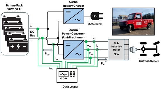
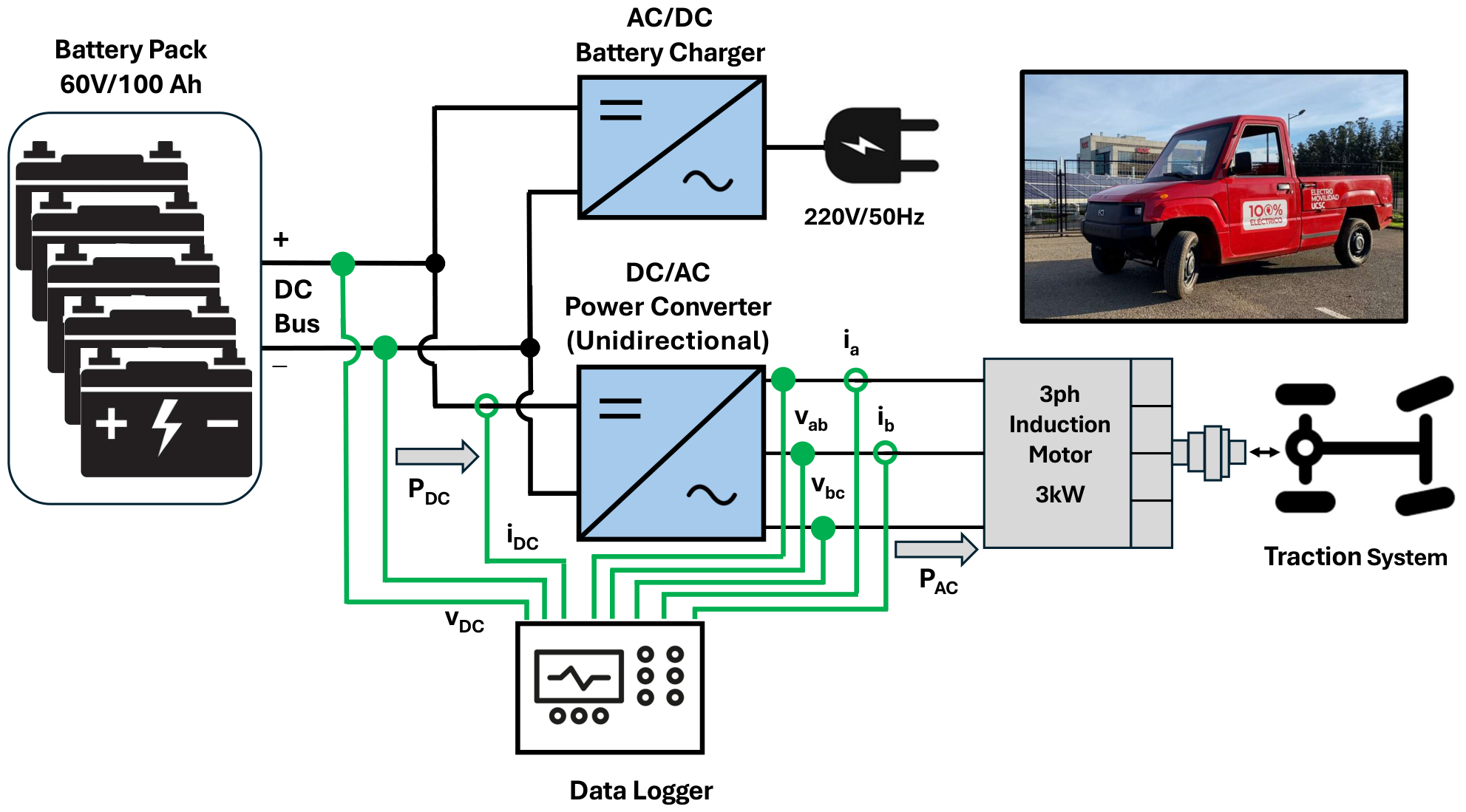
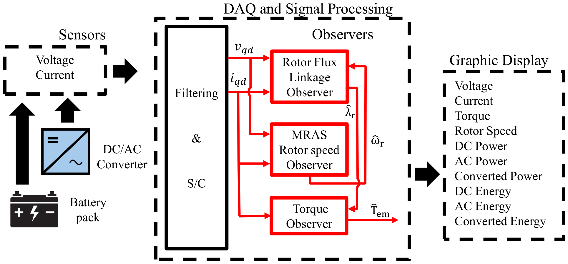
Figure 1 illustrates the powertrain configuration of the SUEV considered in this study, while Figure 2c shows the physical location of its main powertrain components. The vehicle is propelled by a three-phase induction motor coupled to the rear axle through a fixed-ratio mechanical transmission and differential, which deliver the traction torque to the rear wheels. The traction system is supplied by a battery pack through a unidirectional DC/AC inverter. Although the internal control algorithm of the electric drive is not disclosed by the manufacturer, commercial electric vehicles equipped with induction motors typically employ vector control because of its superior dynamic performance and efficiency.

Figure 1. SUEV powertrain scheme including voltage and current data logging system.

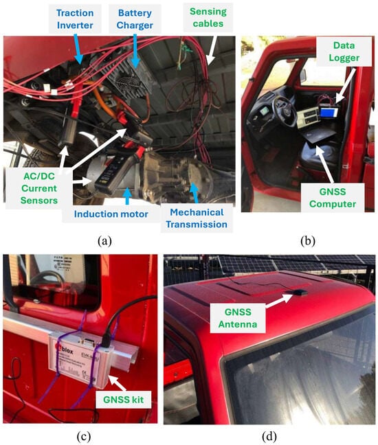
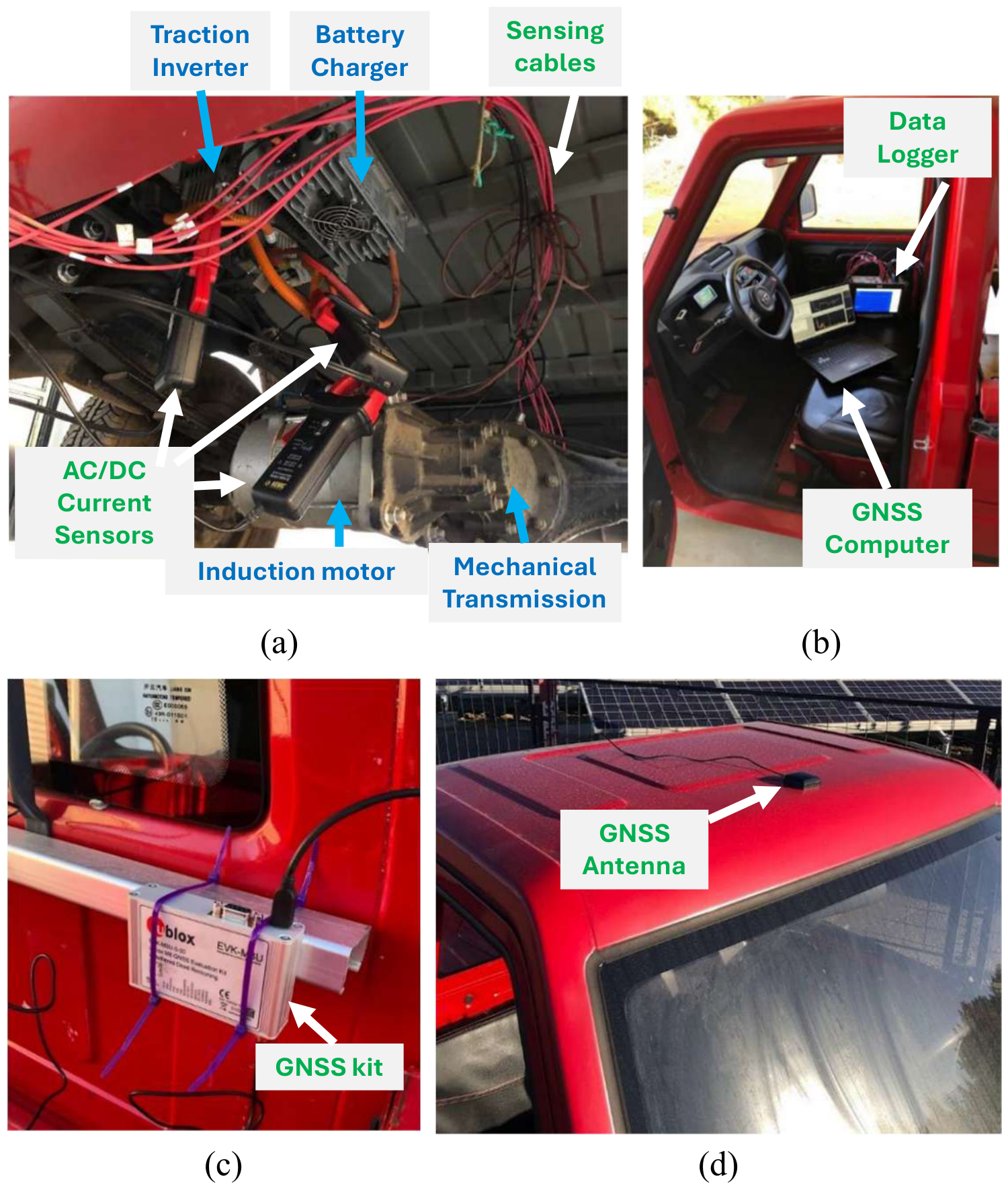
Figure 2. Vehicle and data acquisition system: (a) current sensors mounting, (b) data logger devices mounting, (c) GNSS evaluation kit, (d) GNSS Antenna.

The SUEV was equipped with an onboard data acquisition system that continuously records both electrical and mechanical variables, enabling post-processing analysis of drivetrain performance and energy consumption. The system consists of a high-speed data logger for electrical measurements and a GNSS-based positioning system for vehicle dynamics and route tracking. As illustrated in Figure 1, voltage and current sensors are connected to the onboard data logger through six acquisition channels. Each isolated analog channel has 14-bit resolution and voltage accuracy of 0.1% of full scale ±10 µV. Voltages were measured directly at the recorder inputs, while currents were measured using Hall-effect AC/DC current probes, which have a measurement accuracy lower than 2%. Before each measurement session, the voltage and current channels were zero-adjusted to compensate for offsets.

Three channels are dedicated to voltage measurements, including the DC bus voltage and the AB and BC line voltages of the induction motor. These channels were configured with a measurement range of 200 V and a 1 kHz low-pass filter. Since the voltages are measured directly, no shunt resistors are required. The remaining three channels measure the DC bus current and the line currents in phases A and B of the induction motor. These channels also operate with a 1 kHz low-pass filter and a measurement range of 400 A (AC) to properly capture the traction system current signals. Together, these six electrical measurements provide the input variables required to compute the DC and AC electrical power/energy and to estimate the drivetrain variables using the observer-based methodology described further.

Additional details of the data acquisition system are presented in Figure 2. Figure 2a shows that voltage and current sensors are installed underneath the vehicle, and their output signals are routed through shielded cables to the vehicle cabin, where the onboard data logger is installed (Figure 2b).

In addition to the electrical measurements, a GNSS evaluation kit was used to record the vehicle position and speed during the experiments (see Figure 2c,d). The GNSS module transmits the acquired data to a computer located inside the vehicle cabin (Figure 2b).

The electrical signals were acquired at 50 kHz, while the navigation system provided data at 1 Hz. The two records were manually aligned during post-processing, where the transition from standstill to motion was identified in the electrical signals and the GNSS speed record and used as a common temporal reference.

2.2. Vehicle Load Model

The longitudinal dynamics of electric vehicles have been extensively studied in the literature and provide the basis for evaluating traction requirements under different operating conditions [45,46,47]. In general, the electromagnetic torque delivered by the traction motor must overcome the external resistive forces acting on the vehicle, including the hill-climbing force, rolling resistance, aerodynamic drag, and the inertial force required to accelerate the vehicle when its speed is not constant. The combined effect of these contributions determines the torque demand at the wheels and, consequently, the electrical power required from the drivetrain. The equivalent load torque referred to the motor shaft can be expressed as:

$$\begin{array}{c}\hfill T_{load}={\displaystyle \frac{r_w}{n_{gear}{\eta }_{gear}}}\left[mg\sin \left({\theta }_{road}\right)+{\mu }_{rr}mg\cos \left({\theta }_{road}\right)+{\displaystyle \frac{1}{2}}{\rho }_a{v}^2{C}_{drag}{A}_{SUEV}+ma\right]+J_m{\dot{\omega }}_m\end{array}$$

(1)

where $r_w$ is the wheel radius, $n_{gear}$ is the transmission ratio, m is the total mass of the SUEV, including the transported load, g is the gravitational acceleration, ${\theta }_{road}$ is the road slope angle, ${\mu }_{rr}$ is the rolling resistance coefficient, ${\rho }_a$ is the air density, v is the vehicle speed, $C_{drag}$ is the aerodynamic drag coefficient, A is the frontal area of the SUEV, a is the longitudinal acceleration, $J_m$ is the motor moment of inertia, ${\eta }_{gear}$ is the gear system efficiency, and ${\dot{\omega }}_m$ is the motor angular acceleration.

Here, ${\mu }_{rr}$ represents an effective rolling resistance coefficient, which may vary with tire pressure, load, speed, and tire–road conditions. Equation (1) provides a simplified physical interpretation of traction demand; it is not used to calculate the reported electrical energy consumption or the observer-based motor variables. Tire pressure and payload effects are assessed experimentally through the measured electrical response.

2.3. Routes and Test Protocol

Three predefined routes were established within the university campus to represent controlled and repeatable test scenarios for the experimental evaluation.

• Route 1: corresponds to a flat straight segment shown in Figure 3. The total length of this route is approximately 110 m, with the vehicle starting from rest at Point 1 and accelerating until reaching a constant speed of 10 km/h. Upon reaching Point 2, the vehicle continues accelerating until achieving the maximum speed within the segment, maintaining this condition until Point 3. At this point, the braking system is applied to bring the vehicle to a complete stop. After stopping, the vehicle performs a reverse maneuver, maintaining a constant speed of 10 km/h as indicated on the speedometer, until reaching Point 4, where the vehicle stops and data recording is finalized.
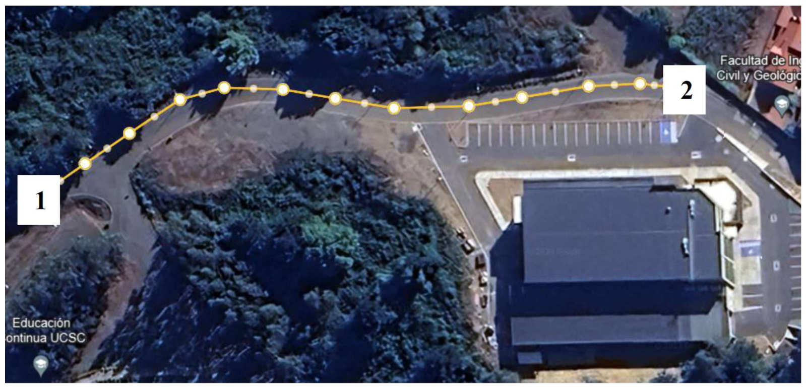
• Route 2: Represents an uphill trajectory along an inclined plane shown in Figure 4. This route has an approximate length of 150 m and an inclination of 18.4°, where the vehicle starts from rest at Point 1 and proceeds uphill until reaching Point 2. During the entire ascent, the accelerator pedal is continuously engaged to maintain sufficient traction force and ensure completion of the climb.
• Route 3: follows the reverse direction of Route 2, representing a downhill trajectory along the same inclined plane. The vehicle starts from Point 2 and descends toward Point 1, where it comes to a complete stop. During this descent, the accelerator pedal is applied only until the vehicle reaches a target speed of 10 km/h, as indicated on the speedometer. After reaching this speed, the vehicle maintains controlled motion along the slope until the endpoint is reached.

Figure 3. Satellite image of Route 1. forward travel from point 1 through point 2 to a complete stop at point 3, followed by reverse travel to point 4.

Figure 3. Satellite image of Route 1. forward travel from point 1 through point 2 to a complete stop at point 3, followed by reverse travel to point 4.

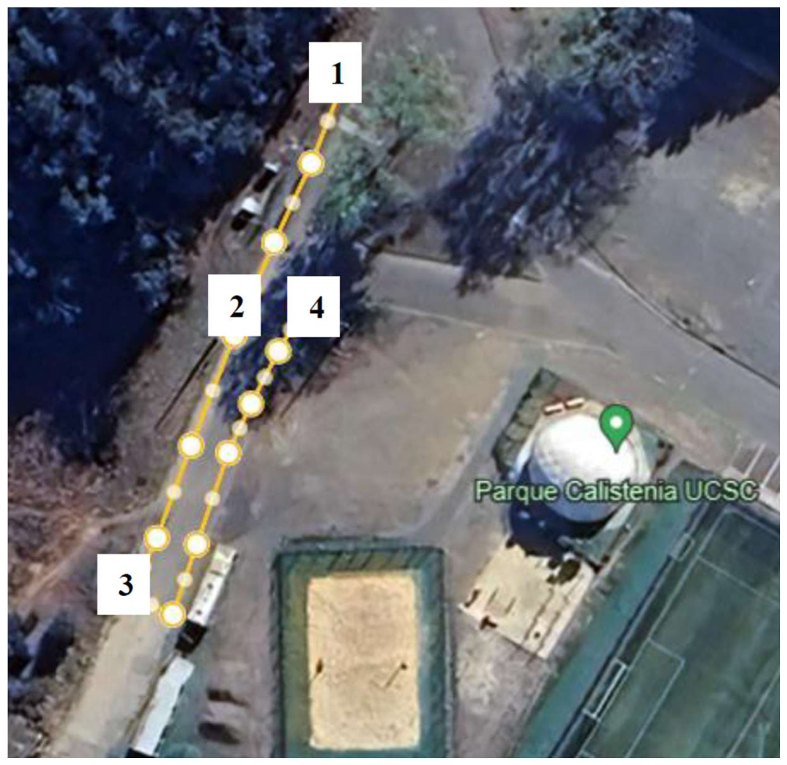
Figure 4. Satellite image of Route 2 and 3. Forward travel from point 1 to point 2 for route 2 and forward travel from point 2 to point 1 for route 3.

Figure 4. Satellite image of Route 2 and 3. Forward travel from point 1 to point 2 for route 2 and forward travel from point 2 to point 1 for route 3.

The same driver operated the vehicle throughout the experiments and underwent practice runs to reproduce similar driving profiles. Several runs were conducted under different tire pressure and payload conditions, and vehicle speed was used as a criterion for selecting comparable runs for the analysis. These measures aimed to reduce variability associated with driving behavior; however, manual operation did not ensure identical speed, acceleration, or braking profiles. The reported results correspond to selected individual runs rather than statistical averages of independent repetitions for each condition.

The dynamic performance test of the SUEV was conducted to evaluate the influence of tire pressure and payload conditions on energy consumption. Four tire pressure levels were considered: 44 psi (manufacturer-recommended pressure), 33 psi, 22 psi, and 10 psi, representing a progressive reduction in tire inflation conditions.

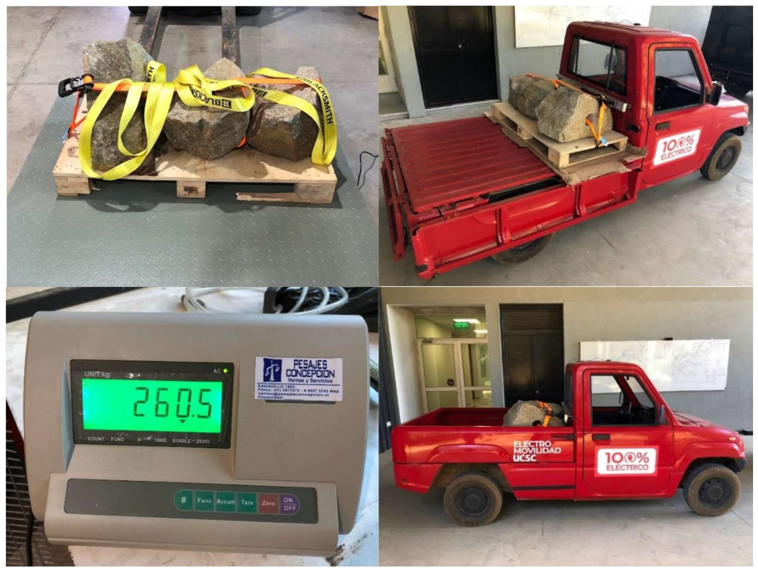
In addition to tire pressure variation, two payload configurations were defined. The first configuration corresponds to the vehicle operated solely by the driver, with an approximate mass of 75 kg. The second configuration includes the driver and an additional load of 260.5 kg placed in the pickup bed. The loaded vehicle used during the experiments is shown in Figure 5.

Figure 5. SUEV under loaded condition.

Figure 5. SUEV under loaded condition.

2.4. Signal Processing and Physics-Based Virtual Sensing

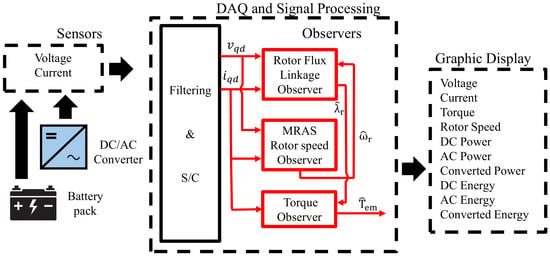
In addition to direct measurements obtained from the onboard monitoring system, observer-based estimation techniques were implemented to reconstruct internal drivetrain variables that were not directly measurable. The estimation strategy is based on the dynamic model of the three-phase induction motor represented in a stationary qd reference frame obtained through Clarke transformation. Using the measured stator voltages and currents, the observers described in [30] simultaneously estimate the rotor flux linkage, rotor speed, and electromagnetic torque. These estimated variables are subsequently used to compute the converted mechanical power.

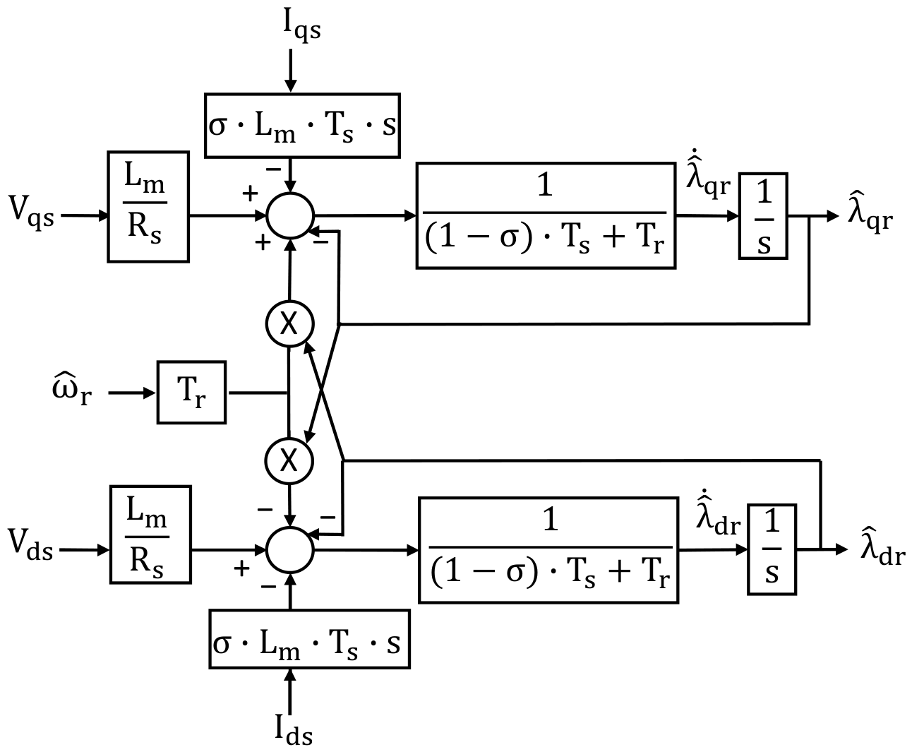
Figure 6 shows the schematic diagram of the three observers implemented for flux, electrical rotor speed and torque estimation.

Figure 6. Rotor flux linkage (RFLO), torque, and rotor speed (MRAS-BEMF) schematic diagram.

2.4.1. MRAS-BEMF Rotor Speed Observer

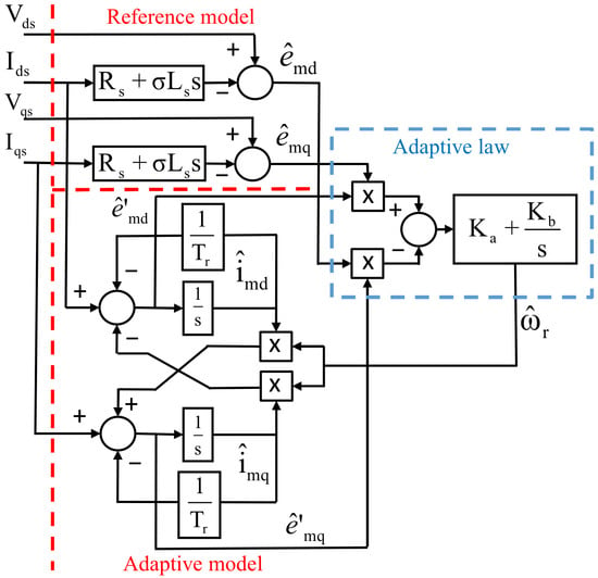
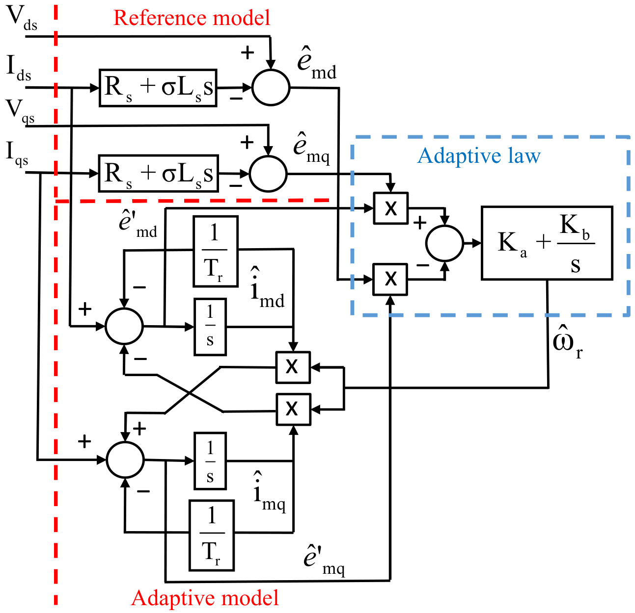
Rotor electrical speed estimation is performed using a Model Reference Adaptive System (MRAS) observer derived from the Back ElectroMotive Force (BEMF) signal obtained from the induction motor dynamic equations. The observer combines a reference model independent of rotor speed with an adaptive model that incorporates the estimated speed as a state variable. The reference model is obtained from the voltage model equations, while the adaptive model is derived from the current model equations of the motor in a stationary qd reference frame. The BEMF components from the voltage model are obtained as:

$${\widehat{e}}_{mq}=v_{qs}-R_s{i}_{qs}-\sigma L_s{\displaystyle \frac{d{i}_{qs}}{dt}}$$

(2)

$${\widehat{e}}_{md}=v_{ds}-R_s{i}_{ds}-\sigma L_s{\displaystyle \frac{d{i}_{ds}}{dt}}$$

(3)

where $v_{qs}$ and $v_{ds}$ are the stator voltage components, $i_{qs}$ and $i_{ds}$ are the stator current components, $R_s$ is the stator resistance, $L_s$ is the stator inductance and $\sigma$ is leakage coefficient.

From the current model, the BEMF components corresponding to the adaptive model are obtained as follows:

$${\widehat{e}}_{mq}^{\prime }={\displaystyle \frac{L_m^2}{L_r}}\left[{\displaystyle \frac{1}{T_r}}\left(i_{qs}-i_{mq}\right)-{\widehat{\omega }}_r{i}_{md}\right]$$

(4)

$${\widehat{e}}_{md}^{\prime }={\displaystyle \frac{L_m^2}{L_r}}\left[{\displaystyle \frac{1}{T_r}}\left(i_{ds}-i_{md}\right)+{\widehat{\omega }}_r{i}_{mq}\right]$$

(5)

where $i_{mq}$ and $i_{md}$ are the magnetizing current components, $L_m$ is mutual inductance, $L_r$ is rotor inductance and $T_r$ is the rotor time constant.

Then, the adaptive law is built as:

$${\widehat{\omega }}_r=\left(K_p+{\displaystyle \frac{K_i}{s}}\right)\left({\widehat{e}}_{md}^{\prime }{\widehat{e}}_{mq}-{\widehat{e}}_{mq}^{\prime }{\widehat{e}}_{md}\right)$$

(6)

where ${\widehat{\omega }}_r$ is the estimated electrical rotor angular speed and $K_p$ and $K_i$ are proportional and integral gains of the adaptive law. Figure 7 shows the block diagram of the implemented MRAS-BEMF rotor speed observer. For simplicity, the factor $L_m^2/L_r$ has been incorporated into the controller gains.

Figure 7. Block diagram of the MRAS-BEMF rotor speed observer (from [30]).

2.4.2. Rotor Flux Linkage Estimation

Several approaches can be used to estimate the rotor flux linkages (RFL) of an induction motor. In this work, a combined voltage-current model observer is adopted due to its improved robustness against parameter variations. In particular, this observer structure reduces the influence of temperature-dependent resistance variations on the rotor flux linkage estimation, resulting in negligible estimation errors under varying operating conditions [33].

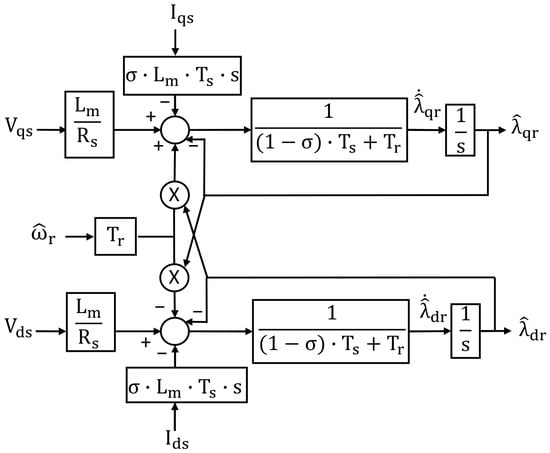
For this model, the rotor flux linkage dynamics in a stationary reference frame are represented as

$${\displaystyle \frac{d{\widehat{\lambda }}_{qr}}{dt}}={\displaystyle \frac{1}{\left[(1-\sigma )T_s+T_r\right]}}\left({\displaystyle \frac{L_m}{R_s}}{v}_{qs}+{\widehat{\omega }}_r{T}_r{\widehat{\lambda }}_{dr}-{\widehat{\lambda }}_{qr}-\sigma L_m{T}_s{\displaystyle \frac{d{i}_{qs}}{dt}}\right)$$

(7)

$${\displaystyle \frac{d{\widehat{\lambda }}_{dr}}{dt}}={\displaystyle \frac{1}{\left[(1-\sigma )T_s+T_r\right]}}\left({\displaystyle \frac{L_m}{R_s}}{v}_{ds}-{\widehat{\omega }}_r{T}_r{\widehat{\lambda }}_{qr}-{\widehat{\lambda }}_{dr}-\sigma L_m{T}_s{\displaystyle \frac{d{i}_{ds}}{dt}}\right)$$

(8)

where ${\widehat{\lambda }}_{qr}$, ${\widehat{\lambda }}_{dr}$ are the rotor flux linkage components, and $T_s$ is the stator time constant.

Figure 8 shows the block diagram of the RFL-Observer. It should be noted that this observer requires the rotor electrical speed signal ${\widehat{\omega }}_r$, which is estimated by the MRAS-BEMF rotor speed observer previously described.

Figure 8. Block diagram of the RFL observer (from [30]).

The electromagnetic torque is estimated from the rotor flux linkage and stator current components according to

$${\widehat{T}}_{em}={\displaystyle \frac{3}{2}}{\displaystyle \frac{P}{2}}{\displaystyle \frac{L_m}{L_r}}\left({\widehat{\lambda }}_{dr}{i}_{qs}-{\widehat{\lambda }}_{qr}{i}_{ds}\right)$$

(9)

where P is the number of poles, ${\widehat{\lambda }}_{dr}$ and ${\widehat{\lambda }}_{qr}$ are the estimated rotor flux linkage components, and $i_{qs}$ and $i_{ds}$ are the stator current components.

The implementation of the three observers described in this section requires prior knowledge of the induction motor parameters. In this study, these parameters were obtained through a motor identification routine executed using the proprietary software provided for an industrial motor drive. This procedure allows the estimation of key electrical and mechanical parameters required for accurate observer performance. A detailed description of the observer-based parameter estimation methodology used in this study can be found in [30]. The identified parameters, along with the main motor specifications, are summarized in Table 1.

Table 1. Induction motor parameters.

Parameter	Value
Rated power	3 kW
Rated speed	3000 rpm
Rated voltage	42 V
Rated frequency	102 Hz
Number of poles (P)	4
Stator resistance (Rs)	0.01524 $\mathrm{\Omega }$
Rotor resistance (Rr)	0.0754 $\mathrm{\Omega }$
Stator leakage inductance (Lls)	0.1094 mH
Rotor leakage inductance (Llr)	0.1170 mH
Magnetizing inductance (Lm)	1.836 mH

2.4.3. Power, Energy and Normalized Indicators

Using the estimated electromagnetic torque and the mechanical rotor speed obtained from the virtual sensing stage, the converted mechanical power is calculated as

$$P_{conv}={\widehat{T}}_{em}{\widehat{\omega }}_m$$

(10)

where the estimated mechanical rotor speed ${\widehat{\omega }}_m$ is obtained from the estimated electrical rotor speed as

$${\widehat{\omega }}_m={\displaystyle \frac{2}{P}}{\widehat{\omega }}_r$$

(11)

Figure 6 shows that voltage and current signals are acquired through sensors and processed by the data acquisition (DAQ) system. These signals are also used to compute the electrical power at both DC and AC sides of the traction system. The DC power is calculated as:

$$P_{DC}=V_{DC}·I_{DC}$$

(12)

where $V_{DC}$ and $I_{DC}$ correspond to the DC bus voltage and current (battery pack output), respectively.

The AC power is obtained from qd voltages and current components as:

$$P_{AC}={\displaystyle \frac{3}{2}}\left(v_{qs}{i}_{qs}+v_{ds}{i}_{ds}\right)$$

(13)

The corresponding energy quantities are obtained through time integration of the power signals:

$$E_{DC}=\int P_{DC}dt$$

(14)

$$E_{AC}=\int P_{AC}dt$$

(15)

$$E_{conv}=\int P_{conv}dt$$

(16)

In cases where the route distance d is expressed in meters and the DC energy $E_{DC}$ in watt-hours, the normalized energy consumption is defined as:

$$E_{DC,N}[\mathrm{kWh}/100\mathrm{km}]=100\times E_{DC}\left[\mathrm{Wh}\right]/d\left[\mathrm{m}\right]$$

(17)

To distinguish the electrical transfer and electromechanical conversion stages, two additional route-integrated indicators are defined:

$${\eta }_{\mathrm{DC}\text{-}\mathrm{AC}}={\displaystyle \frac{E_{\mathrm{AC}}}{E_{\mathrm{DC}}}}\times 100,{\eta }_{\mathrm{AC}\text{-}\mathrm{conv}}={\displaystyle \frac{E_{\mathrm{conv}}}{E_{\mathrm{AC}}}}\times 100.$$

(18)

The first indicator characterizes energy transfer between the measured DC and AC boundaries, while the second describes the estimated conversion of motor electrical input into developed mechanical energy.

An additional global indicator is defined for performance assessment during experimental testing. The DC-to-conversion efficiency is defined as:

$${\eta }_{DC\text{-}conv}={\eta }_{DC\text{-}AC}\times {\eta }_{AC\text{-}conv}={\displaystyle \frac{E_{conv}}{E_{DC}}}\times 100$$

(19)

which provides a comparative assessment of the drivetrain performance from the battery to the motor shaft. Since converted power is calculated from electromagnetic torque and rotor speed, it does not represent useful shaft power after mechanical losses.

2.5. Transmission Ratio Estimation

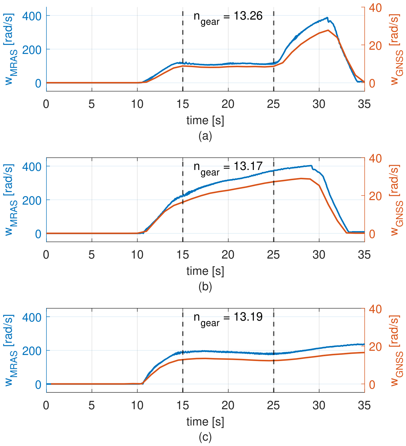
The transmission ratio was identified by comparing the motor speed estimated by the MRAS observer with the vehicle speed obtained from the GNSS module. Since the observer provides the mechanical speed ${\widehat{\omega }}_m$ in rad/s, the GNSS speed was converted from km/h to wheel angular speed in rad/s using the effective wheel radius. The conversion was performed as

$${\omega }_{GNSS}={\displaystyle \frac{v_{GNSS}}{3.6r_{eff}}}$$

(20)

where $v_{GNSS}$ is the vehicle speed in km/h and $r_{eff}$ is the effective wheel radius in meters. Once both variables were expressed in rad/s, the transmission ratio was estimated as

$${\widehat{n}}_{gear}={\displaystyle \frac{{\widehat{\omega }}_m}{{\omega }_{GNSS}}}$$

(21)

2.6. Battery Tests

The electrical power and energy delivered by the battery are calculated as shown in Equations (12) and (14), respectively. These variables are used throughout the experimental analysis to evaluate vehicle autonomy and drivetrain energy consumption under different evaluated scenarios.

During vehicle operation (discharge phase), the electrical power, vehicle speed, traveled distance, and terrain elevation were continuously recorded using the onboard data acquisition system. These measurements allowed the assessment of energy usage under real driving conditions, as well as the correlation between energy consumption, route profile, and vehicle dynamics.

For the charging phase, the vehicle was connected to its standard charging system, and the entire charging process was monitored. Electrical variables including battery voltage, charging current, instantaneous power, and accumulated energy were recorded throughout the charging cycle. In addition, battery temperature was continuously measured to evaluate thermal behavior during the charging process.

3. Results

This section summarizes the results of the experimental data collected after the signal conditioning process described in the previous section.

3.1. Baseline Route Characterization

This subsection presents the baseline results for the three predefined routes under nominal tire pressure (44 psi), with only the driver onboard and no additional payload in the pickup. The analysis includes the evaluation of observer-based electromagnetic torque ${\widehat{T}}_{em}$ and motor speed ${\widehat{\omega }}_m$ (in rpm), together with $P_{DC}$, $P_{AC}$, and $P_{conv}$, as well as the vehicle speed $v_{GNSS}$ obtained from the GNSS module. The corresponding energy quantities, $E_{DC}$, $E_{AC}$, and $E_{conv}$, calculated through numerical integration of the power signals, are also included.

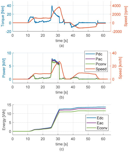
Figure 9 presents the baseline characterization of Route 1. As shown in Figure 9a, the estimated electromagnetic torque ${\widehat{T}}_{em}$ and motor speed ${\widehat{\omega }}_m$ exhibit clearly defined operating phases. During the initial acceleration stage ($t\approx 10$–15 s), the torque gradually increases to 13.5 Nm while the motor speed rises from zero to about 1109 rpm. This is followed by a quasi-steady region between $t\approx 15$–25 s, where both torque and speed remain relatively stable. A second acceleration stage is observed between $t\approx 25$–31 s, characterized by a sharp increase in torque reaching peak values close to 39.2 Nm, accompanied by a rapid rise in motor speed up to 3696 rpm. At the onset of braking ($t\approx 31$–34 s), the torque rapidly decreases toward zero, followed by a short interval where negative torque values are observed. During the reverse motion phase ($t\approx 38$–57 s), both torque and speed take negative values with lower magnitude compared with forward operation, maintaining a relatively constant profile.

Figure 9. Baseline drivetrain SUEV variables for route 1 (a) ${\widehat{T}}_{em}$ and ${\widehat{\omega }}_m$, (b) $P_{DC}$, $P_{AC}$, $P_{conv}$ and $v_{GNSS}$, (c) $E_{DC}$, $E_{AC}$, and $E_{conv}$.

Figure 9b shows the corresponding power signals and $v_{GNSS}$. The DC power reaches peak values close to 7.8 kW during the second acceleration stage, while $P_{AC}$ and $P_{conv}$ follow similar temporal profiles with lower magnitudes. The vehicle speed increases up to 26.9 km/h during forward motion, followed by a rapid decrease during braking and a subsequent lower speed profile during reverse operation. The GNSS-based speed measurement does not distinguish between forward and reverse motion, in contrast to the observer-based motor speed, which clearly reflects the change in direction through the sign of ${\widehat{\omega }}_m$. Additionally, the power signals remain strictly non-negative throughout the entire cycle due to the absence of regenerative braking in the traction system.

Figure 9c presents the cumulative energy profiles obtained through numerical integration of the power signals. The energy curves increase monotonically over time, with a significant increment during the high-power acceleration phase around $t\approx 25$–31 s. At the end of the route, the total energy values reach 13.7 Wh for $E_{DC}$, 12.8 Wh for $E_{AC}$, and 11.6 Wh for $E_{conv}$, maintaining the relationship $E_{conv}<E_{AC}<E_{DC}$ throughout the entire driving cycle.

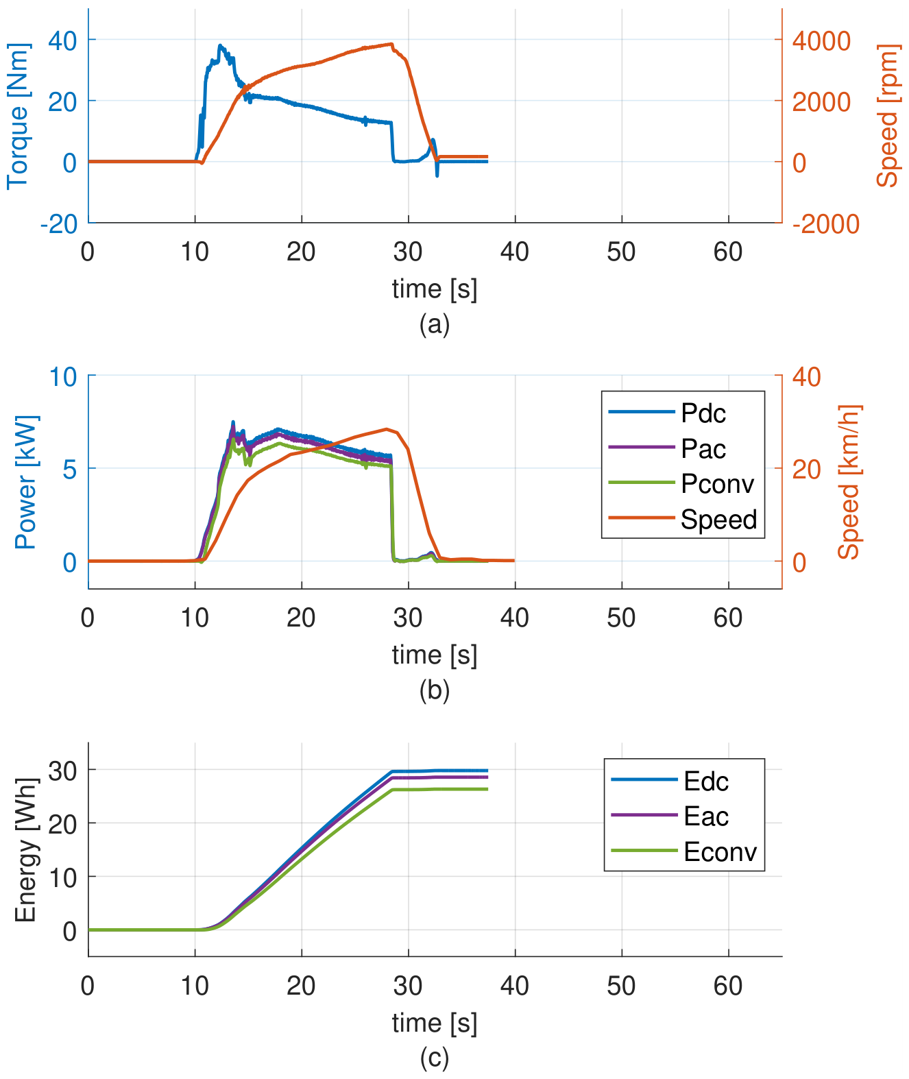
Figure 10 presents the baseline characterization of Route 2.

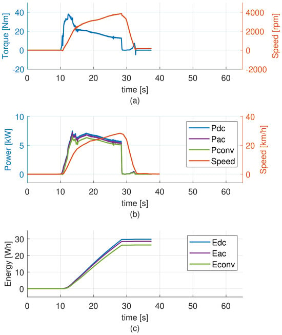
Figure 10. Baseline drivetrain SUEV variables for route 2 (a) ${\widehat{T}}_{em}$ and ${\widehat{\omega }}_m$, (b) $P_{DC}$, $P_{AC}$, $P_{conv}$ and $v_{GNSS}$, (c) $E_{DC}$, $E_{AC}$, and $E_{conv}$.

As shown in Figure 10a, ${\widehat{T}}_{em}$ and ${\widehat{\omega }}_m$ exhibit a sustained high-load operating condition associated with the uphill trajectory. Compared with Route 1, Route 2 has a shorter driving distance and, consequently, a shorter time scale. During the initial acceleration phase ($t\approx 10$–15 s), the torque rapidly increases, reaching peak values close to 37.7 Nm, while the motor speed rises from zero to 1031 rpm. This is followed by a gradual reduction in torque as the speed continues increasing, reaching values close to 3846 rpm. The torque remains positive throughout the ascent, with a slight decreasing trend as the vehicle approaches the end of the route. At the end of the trajectory ($t\approx 30$–32 s), both torque and speed rapidly decrease to zero as the vehicle stops.

Figure 10b shows the corresponding power signals and vehicle speed $v_{GNSS}$. The DC power reaches values between 5.7 and 7.5 kW during the ascent, while $P_{AC}$ and $P_{conv}$ follow similar profiles with lower magnitudes. The vehicle speed increases progressively, reaching 28.3 km/h before decreasing to zero at the end of the route. The power signals remain strictly non-negative throughout the entire cycle due to the absence of regenerative braking.

Figure 10c presents the cumulative energy profiles. The energy curves increase with nearly linear growth during the sustained high power region between $t\approx 10.2$–28.5 s. Despite the shorter distance of Route 2 compared with Route 1, the total energy consumption is higher, reaching 29.8 Wh for $E_{DC}$, 28.6 Wh for $E_{AC}$, and 26.3 Wh for $E_{conv}$.

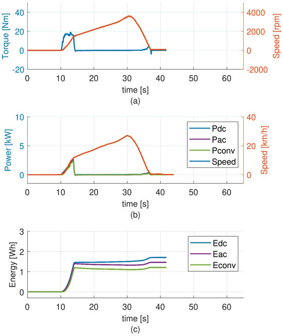
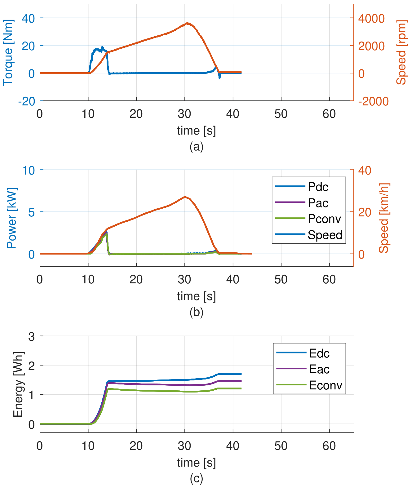
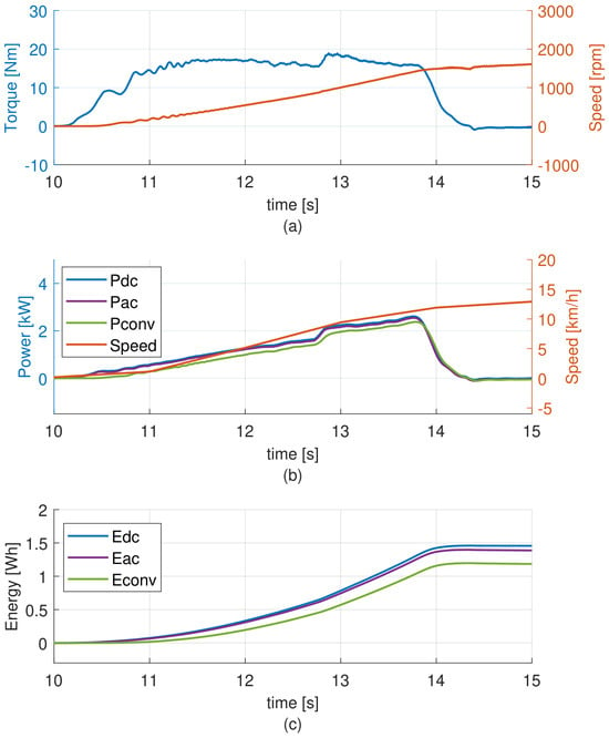
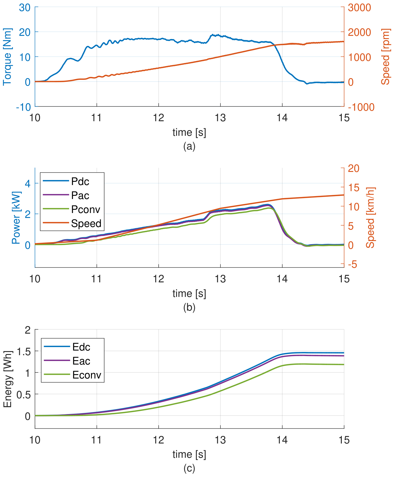
Figure 11 presents the baseline characterization of Route 3, which corresponds to the downhill trajectory evaluated in Route 2. Consequently, although both routes have similar durations and comparable speed profiles, the estimated drivetrain variables ${\widehat{T}}_{em}$ and ${\widehat{\omega }}_r$ exhibit markedly different behavior due to the descending operating conditions. To facilitate the visualization and analysis of the transient response, Figure 12 provides a detailed view of the initial acceleration phase.

Figure 11. Baseline drivetrain SUEV variables for route 3 (a) ${\widehat{T}}_{em}$ and ${\widehat{\omega }}_m$, (b) $P_{DC}$, $P_{AC}$, $P_{conv}$ and $v_{GNSS}$, (c) $E_{DC}$, $E_{AC}$, and $E_{conv}$.

Figure 12. Zoomed view of the baseline drivetrain SUEV variables for route 3 during initial acceleration stage: (a) ${\widehat{T}}_{em}$ and ${\widehat{\omega }}_m$, (b) $P_{DC}$, $P_{AC}$, $P_{conv}$ and $v_{GNSS}$, (c) $E_{DC}$, $E_{AC}$, and $E_{conv}$.

During the initial acceleration period shown in Figure 12 ($t\approx 10$–13.9 s), the estimated torque increases to approximately 17 Nm while the motor speed rises from zero to about 1457 rpm (see Figure 12a). Once the vehicle reaches the downhill section, the required traction torque rapidly decreases to nearly zero and remains at this level for the rest of the route. Meanwhile, the motor speed continues increasing, reaching approximately 27 km/h (see Figure 11b) at $t\approx 30.1$ s due to the gravitational component of the slope.

Despite operating under low torque conditions for most of the trajectory, the observer-based estimations remain stable and consistent, demonstrating their capability to accurately track both torque and speed even when the signals exhibit very low magnitudes. At the end of the route ($t\approx 38$ s), both torque and speed decrease rapidly to zero as the vehicle stops.

It is also observed that at $t\approx 36.6$ s, the torque exhibits a secondary increase, reaching 3.9 Nm, followed by a sharp decrease to $-2.2$ Nm as the vehicle speed approaches zero during braking. This behavior is consistently observed across all analyzed routes, occurring at the end of the braking phase. This phenomenon is further analyzed in the following subsection.

Figure 11b and Figure 12b show the corresponding power signals and $v_{GNSS}$. $P_{DC}$ exhibits a short transient peak during the initial acceleration, followed by significantly lower values compared with Route 2, remaining close to zero during most of the descent. The vehicle speed increases progressively, reaching values close to 26.9 km/h before decreasing to zero at the end of the route. The power signals remain strictly non-negative throughout the entire cycle, demonstrating the absence of regenerative braking.

Figure 11c and Figure 12c present the cumulative energy profiles. The energy curves increase rapidly during the initial acceleration phase and then exhibit a very slow growth during the remainder of the trajectory. Despite having a similar duration and speed profile compared with Route 2, the total energy consumption is significantly lower, reaching 1.7 Wh for $E_{DC}$, 1.46 Wh for $E_{AC}$, and 1.2 Wh for $E_{conv}$, consistent with the contribution of gravitational forces.

Table 2 summarizes the distance, energy consumption, normalized energy, and conversion efficiency for the three predefined routes under baseline conditions. The reported values correspond to the integrated energy quantities $E_{DC}$, $E_{AC}$, and $E_{conv}$ obtained from the measured and estimated power signals. Additionally, the normalized energy consumption $E_{DC,N}$ and the conversion efficiencies ${\eta }_{AC\text{-}DC}$, ${\eta }_{AC\text{-}conv}$ and ${\eta }_{DC\text{-}conv}$ provide a comparative assessment of the drivetrain performance from the battery to the motor shaft.

Table 2. Comparison of distance, energy consumption, normalized energy, and conversion efficiencies for the three experimental routes under baseline conditions (44 psi, driver only).

Route	Dist. [m]	${\mathit{E}}_{\mathit{DC}}$ [Wh]	${\mathit{E}}_{\mathit{AC}}$ [Wh]	${\mathit{E}}_{\mathit{conv}}$ [Wh]	${\mathit{E}}_{\mathit{DC}\mathbf{,}\mathit{N}}$ [kWh/100 km]	${\mathit{\eta }}_{\mathit{DC}\mathbf{\text{-}}\mathit{AC}}$ [%]	${\mathit{\eta }}_{\mathit{AC}\text{-}\mathit{conv}}$ [%]	${\mathit{\eta }}_{\mathit{DC}\text{-}\mathit{conv}}$ [%]
Route 1	110	13.7	12.8	11.6	12.42	93.4	90.6	84.6
Route 2	150	29.8	28.6	26.3	19.86	96.0	92.0	88.3
Route 3	150	1.7	1.46	1.2	1.13	85.9	82.2	70.6

The results demonstrate that the energy demand is strongly influenced by the route characteristics. Although Routes 2 and 3 have the same traveled distance, Route 2 exhibits significantly higher energy consumption, indicating the dominant effect of uphill operation. In contrast, Route 3 presents the lowest energy demand, consistent with the assistance provided by gravitational forces during downhill motion. This trend is further confirmed by the normalized energy consumption, where Route 2 shows the highest energy per unit distance, while Route 3 exhibits a substantially lower value.

The DC to conversion efficiency values provide insight into the energy transfer from the battery to the motor shaft. In all cases, the relationship $E_{conv}<E_{AC}<E_{DC}$ is preserved, confirming the presence of electrical and mechanical conversion losses throughout the electric part of the drivetrain. Routes 1 and 2 exhibit relatively high efficiencies, exceeding 84%, indicating effective electromechanical energy conversion under traction-dominated operating conditions. In contrast, Route 3 shows a lower efficiency of 70.6%, despite its reduced energy demand. This behavior is associated with the low torque and power operation during downhill motion, where the motor operates below its nominal current. Under these conditions, the magnetizing current represents a larger fraction of the total current, reducing the overall efficiency of the motor. Additionally, if regenerative braking were implemented, part of this energy could be recovered, potentially improving the overall system efficiency. In all cases, the efficiency values reflect the cumulative effect of losses across the inverter and motor.

The stage-level indicators ${\eta }_{DC\text{-}AC}$ and ${\eta }_{AC\text{-}conv}$ show higher efficiencies during uphill operation than during downhill operation. As expected, the motor’s electromechanical conversion efficiency is lower than the DC-to-AC converter efficiency across all three routes, supporting the physical consistency of the results.

3.2. Electrical Behavior During Braking

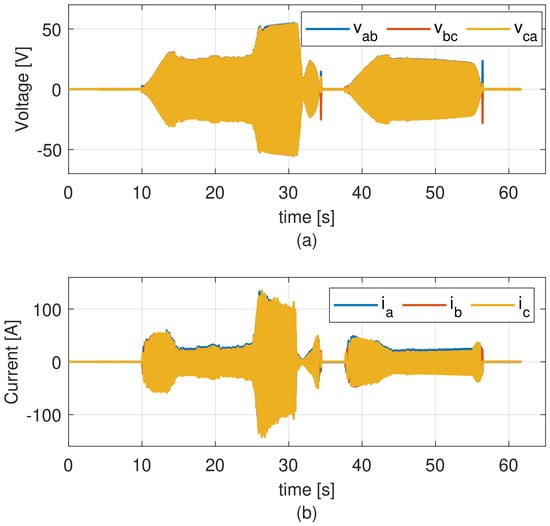
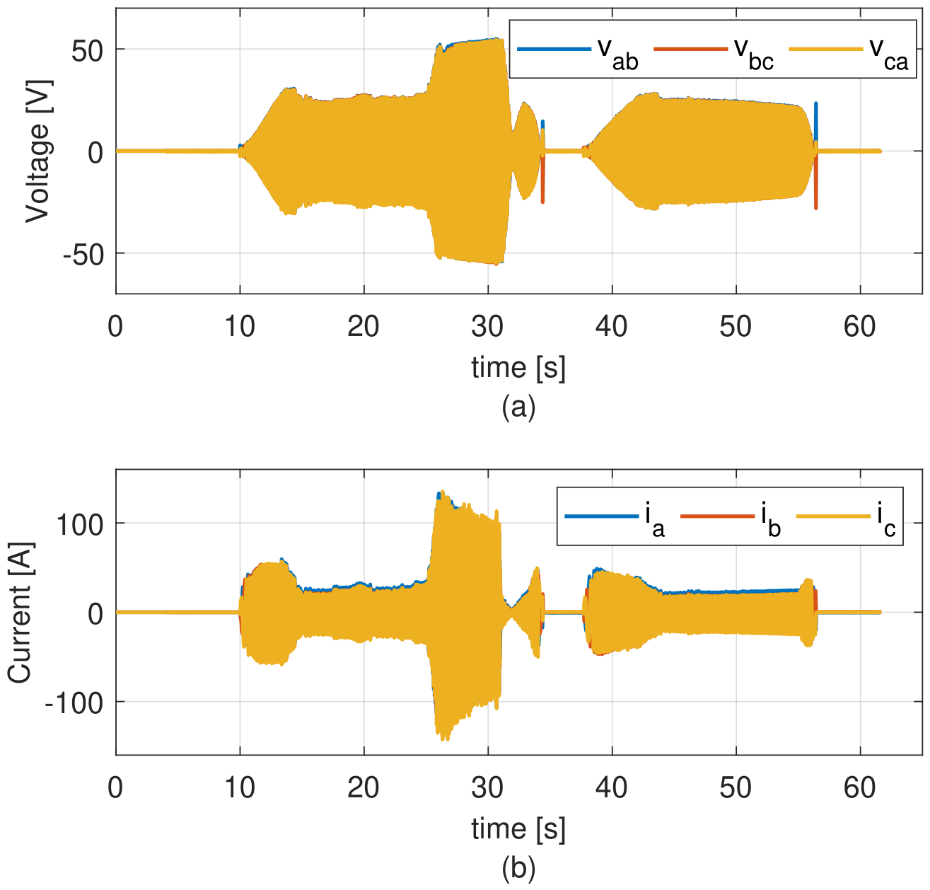
A more detailed analysis is required to characterize the braking behavior observed in the previous subsection, particularly the increase in torque and power when the vehicle speed approaches zero. Additional variables, including the three-phase stator voltages and currents, are analyzed in order to provide a clearer description of the motor operation during braking scenarios. Figure 13 presents the instantaneous three-phase stator voltages and currents measured during Route 1. The line-to-line voltages ($v_{ab}$, $v_{bc}$, and $v_{ca}$) and phase currents ($i_a$, $i_b$, and $i_c$) exhibit a balanced three-phase waveform with alternating polarity, maintaining consistent amplitude throughout most of the operating cycle. Variations in amplitude can be observed during the different driving phases, particularly during acceleration and braking intervals. Near the first braking interval between $t\approx 31$–34 s, noticeable changes in the current waveform are observed, including variations in amplitude and waveform shape. In particular, at $t\approx 34$ s, the currents exhibit a significant increase, coincident with the torque reaching 7.7 Nm as the vehicle speed approaches zero (see Figure 9a).

Figure 13. Instantaneous motor voltages and currents for Route 1: (a) line-to-line voltages and (b) phase currents.

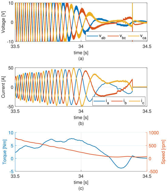
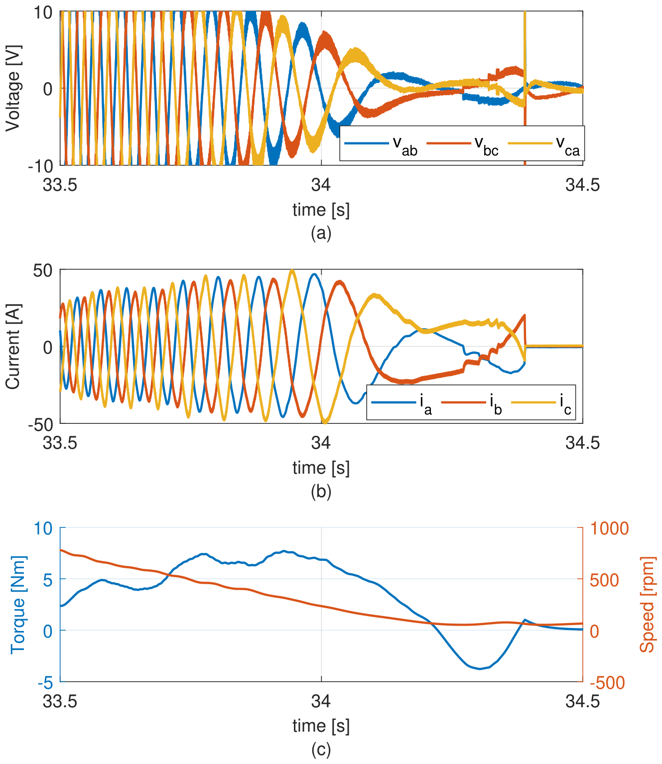
Figure 14 presents a detailed view of the braking interval between 33.5 and 34.5 s, including voltages, currents, torque, and motor speed. Figure 14b shows a significant increase in current, reaching peak values close to 50 A at $t\approx 34$ s, even while the voltage amplitudes are decreasing. This behavior is associated with the interaction between the mechanical braking action and the control system. As the vehicle speed decreases faster than the internal speed reference, the controller produces a transient increase in torque demand.

Figure 14. Zoom of motor voltages, currents, torque and motor speed for braking phase of route 1, (a) line voltages and (b) phase currents and (c) torque and motor speed.

From $t\approx 34.2$ s onward, the final stage of braking is observed. Figure 14a shows a change in the voltage sequence, which can be identified by the alteration in the order of peak amplitudes of the line-to-line voltages. This behavior allows identification of the braking strategy implemented in the vehicle, which employs a counter-current braking method. In this approach, two phases of the motor are inverted to generate a braking torque, as shown in Figure 14c, where the torque reaches negative values close to $-3.7$ Nm. This strategy enables faster deceleration and reduces reliance on the mechanical braking system. However, no energy is recovered to the battery during this process, and the electrical energy is dissipated instead. Although this method is not energy efficient, it contributes to reducing the wear of the mechanical braking components.

3.3. Tire Pressure Effects

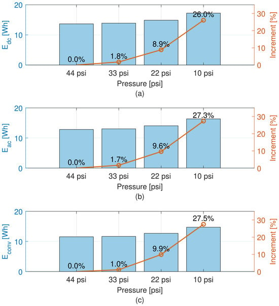
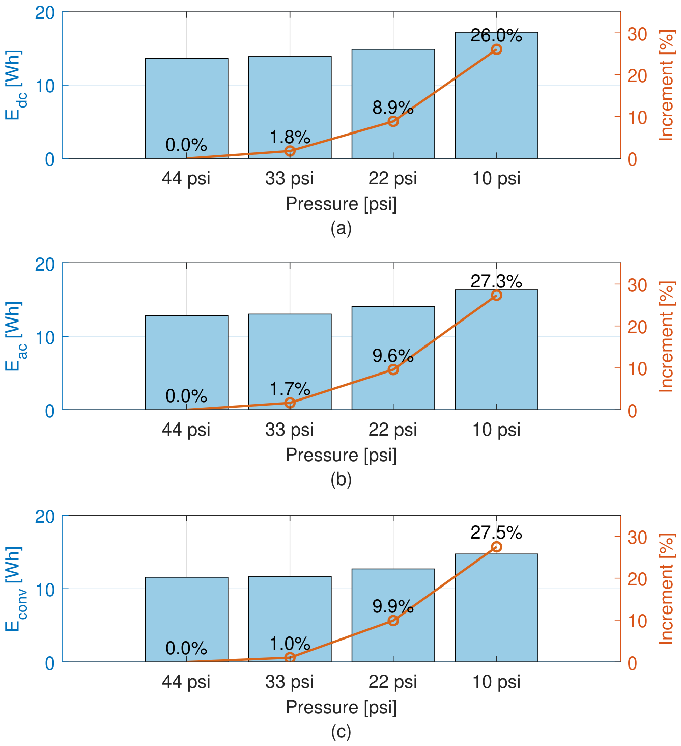
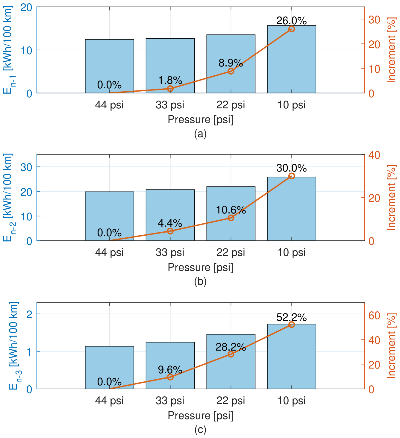
Figure 15 presents the effect of tire pressure on energy consumption for Route 1. As shown in Figure 15a–c, a consistent increase in energy consumption is observed as the tire pressure decreases from 44 psi to 10 psi. The DC energy $E_{DC}$ increases progressively, with a relative increment of 1.8% at 33 psi, 8.9% at 22 psi, and up to 26.0% at 10 psi. A similar trend is observed for $E_{AC}$ and $E_{conv}$, where the maximum increments reach 27.3% and 27.5%, respectively.

Figure 15. Energy consumption and relative increment for Route 1 under different tire pressure: (a) $E_{DC}$, (b) $E_{AC}$, and (c) $E_{conv}$.

The results demonstrate that the reduction in tire pressure leads to a systematic increase in energy demand, with a nonlinear behavior that becomes more pronounced at lower pressure levels. While the variation between 44 psi and 33 psi is relatively small, a significant increase in energy consumption is observed below 22 psi. This indicates that tire pressure has a strong influence on the energy efficiency of the vehicle, particularly under low pressure conditions, where the energy demand increases significantly.

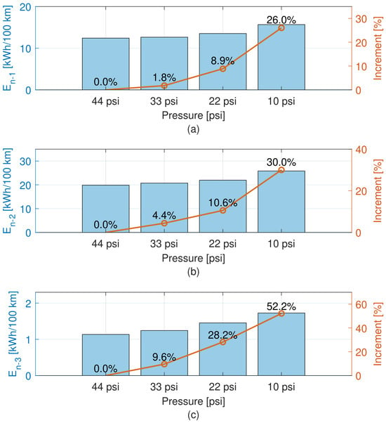
Figure 16 presents the effect of tire pressure on energy consumption for all routes. The results are expressed in terms of normalized DC energy to enable direct comparison across different test conditions, where $E_{n\text{-}1}$, $E_{n\text{-}2}$, and $E_{n\text{-}3}$ correspond to Routes 1, 2, and 3, respectively. A consistent increase in energy demand is observed as the tire pressure decreases from 44 psi to 10 psi in all cases. However, the magnitude of this increase differs significantly between routes.

Figure 16. Normalized $E_{DC,N}$ and relative increment for all routes under different tire pressure: (a) route 1, (b) route 2, and (c) route 3.

For Route 1 (Figure 16a), the energy consumption exhibits a moderate increase, reaching 26.0% at 10 psi. Route 2 (Figure 16b) shows a slightly higher sensitivity, with an increase of up to 30.0%. In contrast, Route 3 (Figure 16c) presents the most pronounced variation, with energy consumption increasing up to 52.2% at the lowest pressure level.

The results indicate that the influence of tire pressure on energy consumption is strongly dependent on the driving conditions, with the downhill route exhibiting the highest relative variation, followed by the uphill and flat routes.

3.4. Payload Effects

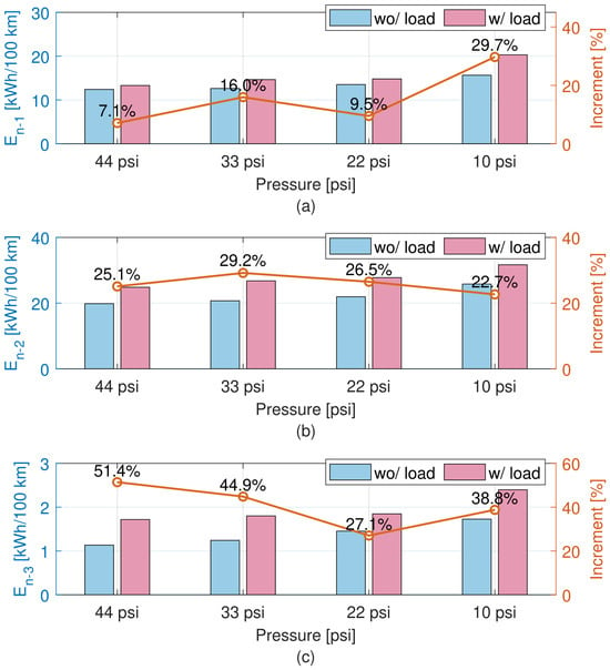
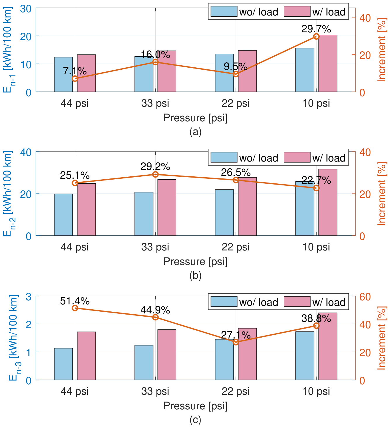
Figure 17 presents the combined effect of tire pressure and transported load on the normalized energy consumption for the three routes. The results compare the unloaded condition (driver only—75 kg) with the loaded condition (driver plus a payload of 260.5 kg), highlighting the additional energy demand introduced by increased transported mass. In this case, the percentage increment shown in the figure is calculated for each tire pressure level with respect to the corresponding unloaded condition, allowing a direct assessment of the isolated effect of transported load at each pressure.

Figure 17. Normalized Energy consumption and relative increment for all Routes considering different tire pressure and transported load conditions: (a) route 1, (b) route 2, and (c) route 3.

For Route 1 (Figure 17a), the presence of additional load leads to a moderate increase in energy consumption across all pressure levels, with relative increments ranging from 7.1% at 44 psi to 29.7% at 10 psi. The influence of the transported load becomes more pronounced as tire pressure decreases, indicating a combined effect between load and rolling resistance.

In Route 2 (Figure 17b), the impact of payload is more significant, with energy increases between 25.1% and 29.2% depending on the pressure level. The variation remains relatively consistent across pressures, suggesting that the additional energy demand is dominated by the increased traction effort required to overcome the inclined route.

For Route 3 (Figure 17c), the effect of payload is highly pronounced at higher tire pressures, reaching up to 51.4% at 44 psi. As the pressure decreases, the relative increment reduces, reaching 27.1% at 22 psi and increasing again to 38.8% at 10 psi. This behavior reflects the sensitivity of low-energy operating conditions to additional mass.

Table 3 summarizes the impact of the combined effect of severe tire underinflation (10 psi) and transported load on normalized energy consumption for the three routes, using the baseline condition (44 psi, no load) as reference. The results indicate a substantial increase in energy demand across all routes, with increments of 63.5% and 59.5% for Routes 1 and 2, respectively. A significantly larger relative increase of 112.4% is observed for Route 3.

Table 3. Impact of combined tire underinflation and transported load on normalized energy consumption.

Route	${\mathit{E}}_{\mathit{DC},\mathit{N}}$ Base [kWh/100 km]	${\mathit{E}}_{\mathit{DC},\mathit{N}}$ Worst [kWh/100 km]	Increase [%]
Route 1	12.42	20.31	63.5%
Route 2	19.86	31.68	59.5%
Route 3	1.13	2.40	112.4%

It should be noted that, due to the significantly lower absolute energy consumption in Route 3 compared with Routes 1 and 2, the relative variations may be more sensitive to measurement uncertainty. Due to the low baseline energy consumption of Route 3, its relative changes are particularly sensitive to measurement uncertainty and should be interpreted cautiously, together with the absolute energy values.

Overall, the results demonstrate that the transported load has a significant impact on energy consumption across all routes, with the magnitude of this effect depending on both tire pressure and driving conditions. The combined influence of reduced tire pressure and increased transported load leads to the highest energy demand, particularly under low-pressure conditions.

3.5. Transmission Ratio Identification

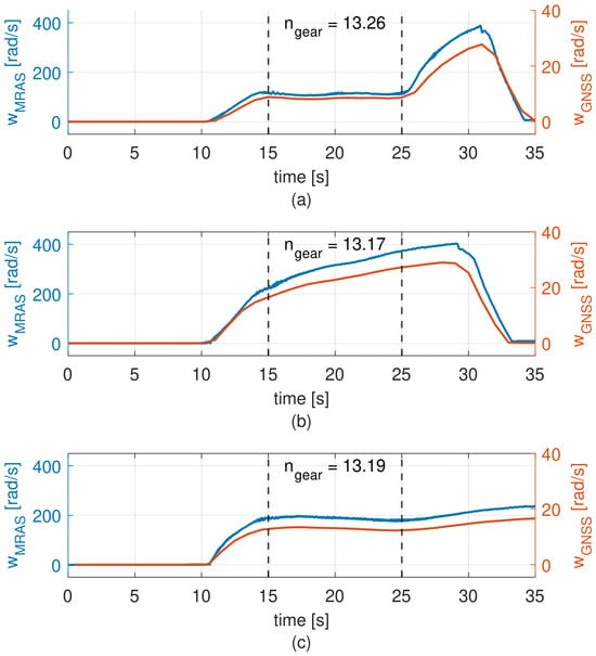
The transmission ratio was calculated only during quasi-steady speed intervals in order to avoid numerical errors associated with rapid transients, where the denominator changes quickly and may produce large fluctuations in the estimated ratio.

Three experimental conditions were considered: 44 psi without transported load, 33 psi without transported load, and 22 psi with additional load. Due to the combined effect of tire pressure and load, the effective wheel radius measured for these tests was 0.27 m, 0.26 m, and 0.245 m, respectively.

Figure 18 presents the corresponding results. In all three cases, ${\omega }_r$ and ${\omega }_{GNSS}$ exhibit similar temporal profiles, differing mainly in magnitude according to the transmission ratio. The steady-state intervals selected for the estimation are indicated by dashed vertical lines. For the test at 44 psi without load (Figure 18a), the identified transmission ratio is 13.26. For the test at 33 psi without load (Figure 18b), the estimated value is 13.17. Finally, for the test at 22 psi with payload (Figure 18c), the estimated transmission ratio is 13.19.

Figure 18. Transmission ratio identification under different test conditions: (a) 44 psi without load, (b) 33 psi without load, and (c) 22 psi with load.

The results show that the identified transmission ratio remains nearly constant despite variations in tire pressure, transported load, and effective wheel radius. The three tests provide very similar values, indicating that the drivetrain presents a stable effective transmission ratio of 13.2:1 under the evaluated operating conditions.

This result is consistent with typical transmission ratios reported by manufacturers of rear axles for SUEVs, where common values include 8.5, 9, 10.5, 13, and 18. The identified value obtained in this study closely matches the nominal ratio of 13, allowing the effective transmission ratio of the tested vehicle to be confidently associated with this configuration. The consistency among the three estimates supports the internal coherence of the proposed identification procedure under the evaluated conditions.

Additionally, the proposed approach has potential applications for drivetrain condition monitoring. Deviations from the nominal transmission ratio could indicate faults or anomalies in the mechanical transmission system, such as slippage, wear, or damage in drivetrain components. Therefore, the proposed identification method could be extended as a diagnostic tool for detecting transmission-related faults during vehicle operation.

3.6. Battery Discharge and Cycle Range

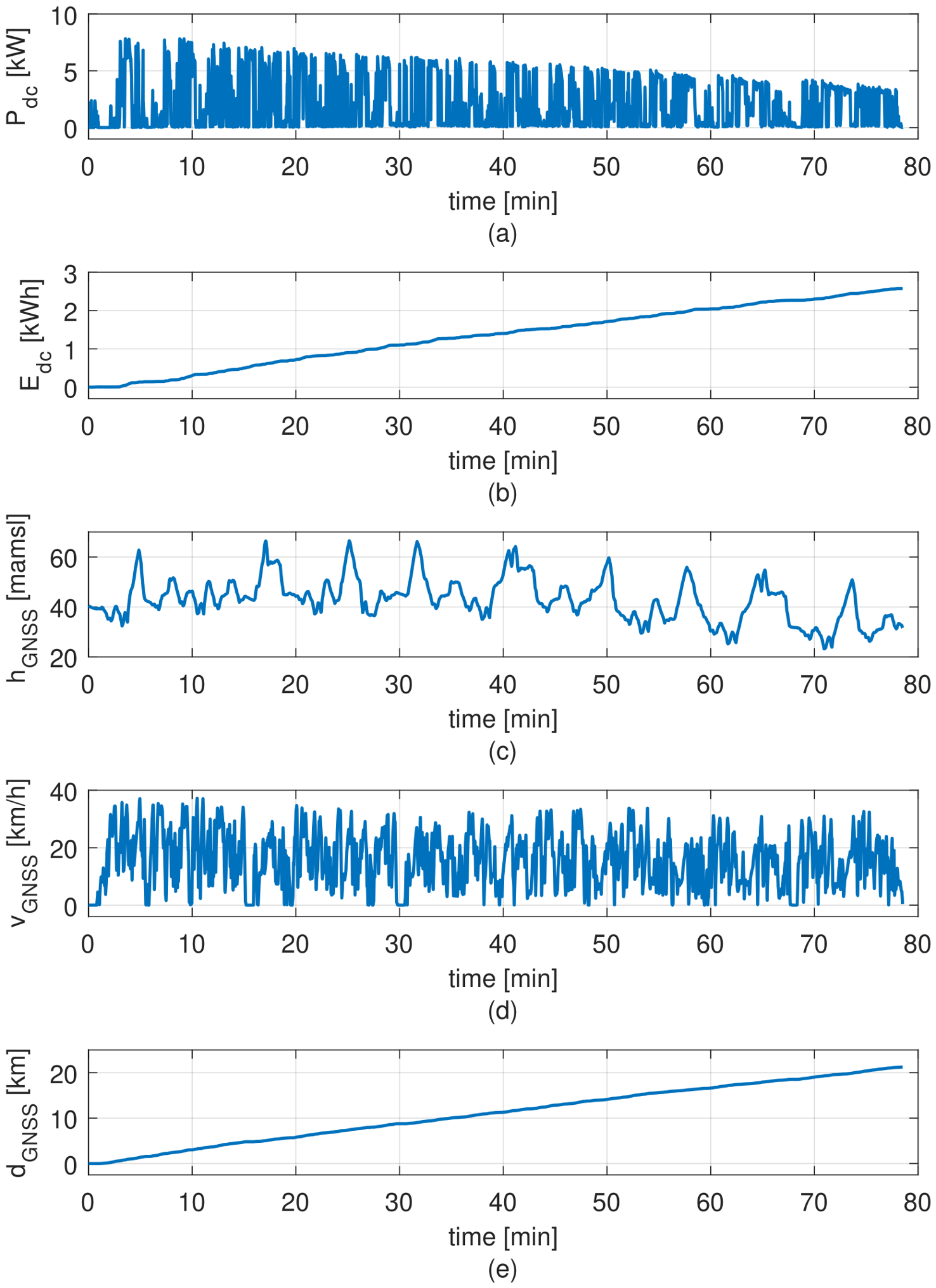
This subsection presents the results of battery discharge tests and vehicle autonomy under repeated driving cycles. The analysis includes DC power, DC energy, GNSS-based altitude, vehicle speed, and traveled distance.

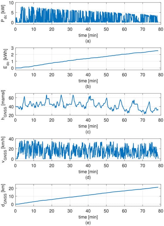
Figure 19 shows the first 78 min of operation, corresponding to repeated circuits within the campus to promote battery discharge and evaluate vehicle autonomy. The battery pack has a nominal capacity of 6 kWh and was fully charged at the beginning of the test, with the SUEV operating without additional load and at 44 psi.

Figure 19. Battery discharge test under repeated driving cycles: (a) DC power, (b) DC energy, (c) GNSS altitude, (d) GNSS vehicle speed, and (e) GNSS traveled distance.

As shown in Figure 19, the power profile exhibits highly dynamic behavior, with frequent fluctuations between low and high power levels, including peaks exceeding 3 kW, which is higher than the motor rated power. This reflects the stop-and-go nature of the driving cycle. It is also observed that the power levels decrease progressively as the battery state of charge is reduced during the test. This behavior is consistent with the characteristics of lead-acid batteries, where the terminal voltage decreases with decreasing state of charge. Consequently, the lower operating voltage reduces the available electrical power, even under similar load conditions. This effect also influences vehicle performance toward the end of the discharge cycle, limiting the achievable speed and acceleration.

Regarding energy consumption (Figure 19b), the accumulated DC energy reaches 2.57 kWh at the end of the evaluated interval, corresponding to approximately 42.8% of the battery pack’s rated energy of 6 kWh. This energy-based indicator provides a practical reference for assessing battery utilization and supporting range estimation under comparable operating conditions. It may approximate SOC depletion when the effective capacity and average discharge voltage remain close to their nominal values; however, it should not be interpreted as a directly measured SOC reduction.

Looking at Figure 19c, the GNSS-based altitude profile shows variations on the order of 15 m; however, a loss of measurement precision is observed over time. These variations are not associated with changes in the route but rather with the inherent accuracy limitations of the GNSS system. Despite this measurement uncertainty, the repeated driving cycles can still be identified, showing that the duration of each cycle increases progressively as the battery discharges. This behavior confirms the previously observed reduction in available power at lower states of charge, which results in longer travel times for similar driving conditions.

Similarly, the vehicle speed profile (Figure 19d) exhibits significant variability, with peaks close to 37 km/h and frequent accelerations and decelerations, consistent with urban driving conditions. Additionally, a progressive reduction in the peak vehicle speed is observed as the state of charge decreases. This behavior is consistent with the reduction in available power and further confirms the impact of battery discharge on vehicle performance. As the available voltage and current decrease, the delivered power is reduced, and the vehicle is no longer able to reach the same speed levels under similar driving conditions. This observation is consistent with the increase in cycle duration and reinforces the overall effect of battery characteristics on the dynamic response of the vehicle.

Finally, the traveled distance (Figure 19e) increases steadily, reaching 21.2 km after 78 min of operation, corresponding to a normalized energy of 12.12 kWh/100 km.

The results indicate that the vehicle operates under realistic and highly transient conditions, where energy consumption is influenced by both driving dynamics and terrain variations. Using the rated battery energy of 6 kWh and the measured consumption of 2.57 kWh over 21.2 km, the extrapolated range under comparable operating conditions is approximately 49.5 km, assuming that the rated energy is fully usable. This value is in close agreement with the measured value of 51 km.

3.7. Charging Profile Characterization

This subsection presents the voltage, current, power, accumulated energy, and temperature profiles during the battery charging process.

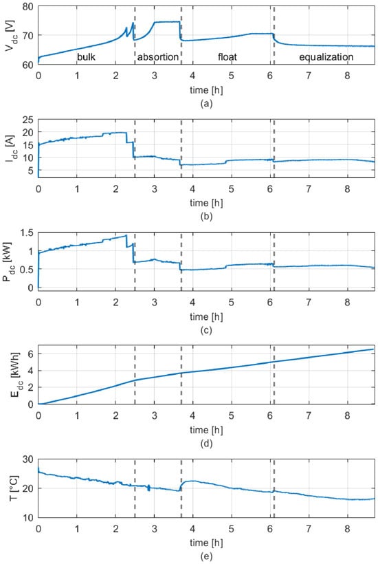
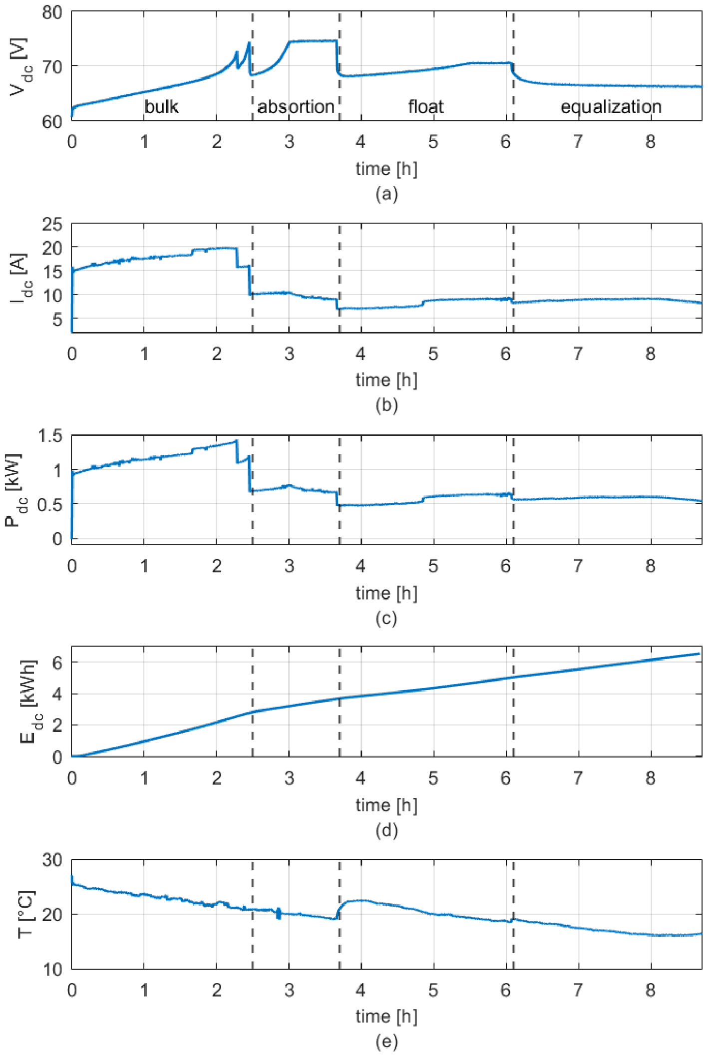
As shown in Figure 20, the charging process exhibits the characteristic stages of lead-acid battery charging. During the initial stage (0–2.5 h), the charging current remains nearly constant at a high level, corresponding to the bulk stage. In this period, the voltage increases gradually from 62 V to around 74 V, while the charging power reaches its highest levels, close to 1.35 kW.

Figure 20. Battery charging profile: (a) DC voltage, (b) DC current, (c) DC power, (d) DC energy, and (e) temperature as a function of time.

Between 2.5 h and 3.7 h, the absorption stage takes place. In this interval, the voltage increases slowly up to 74 V and is then regulated near this value, while the current decreases progressively around 10 A. This results in a noticeable reduction in charging power compared with the bulk stage.

After 3.7 h, the float stage begins and extends until around 6.1 h. During this stage, the power remains practically constant around 0.6 kW while the voltage increases slowly and stabilizes at 70 V. In this stage, current remains low and nearly constant, indicating that the battery is approaching full charge.

From 6.1 h onward, an additional stage is observed where the voltage is regulated near 66 V and the current remains at 8.6 A, corresponding to the equalization or final charging stage. This stage continues until the end of the process at 8.7 h.

The accumulated energy increases throughout the charging process, with a higher slope during the bulk stage due to the elevated charging power. As the process transitions into the absorption and float stages, the rate of energy accumulation decreases, reflecting the reduction in current and power. At the end of the charging process, the total accumulated energy reaches 6.5 kWh, which is slightly higher than the rated battery capacity due to charging losses and conversion inefficiencies.

The temperature profile shows an initial decrease from 27.2 °C to 18.9 °C during the early stages of the charging process. Since ambient temperature was not independently monitored, the observed trend cannot be attributed exclusively to battery-internal phenomena and is likely influenced by heat exchange with the surrounding environment. Despite the relatively high currents during the bulk and absorption stages, no significant sustained temperature increase is observed, indicating stable thermal behavior throughout most of the charging process. However, at the beginning of the float stage, the noticeable increase in temperature can be attributed to the thermal inertia of the battery, where heat generated during the previous charging stages continues to propagate within the system. As the charging current decreases during the float stage, heat generation is reduced while heat dissipation becomes dominant, leading to a gradual decrease in temperature [48].

4. Discussion

The results provide a comprehensive characterization of the drivetrain and energy performance of the SUEV under real operating conditions. Energy consumption is strongly influenced by route characteristics, with elevation playing a dominant role. The comparison between uphill and downhill operation confirms the significant impact of gravitational forces, while the absence of regenerative braking leads to energy dissipation during deceleration, limiting overall efficiency.

The drivetrain exhibits high conversion efficiency under traction-dominated conditions, exceeding 80% for flat and uphill routes. However, efficiency decreases during low-torque operation, where magnetizing current becomes dominant, increasing relative losses. This highlights the dependence of motor efficiency on the operating point.

The braking analysis reveals a strong interaction between control strategy and mechanical dynamics, with transient increases in torque and current near zero speed. The use of counter-current braking enables effective deceleration but results in energy dissipation rather than recovery.

Tire pressure has a significant and nonlinear impact on energy consumption, with severe underinflation producing substantial increases due to higher rolling resistance. The transported load further increases energy demand, particularly in uphill conditions, confirming the combined influence of mass and tire deformation on traction requirements.

The virtual sensing approach enables electrical measurements to be translated into estimated mechanical variables, facilitating detailed drivetrain analysis without direct mechanical sensing. This enables the estimation of internal drivetrain variables and the identification of the transmission ratio, which remained consistent across the experimental conditions.

Battery performance plays a critical role in vehicle operation, as the reduction in stored energy leads to lower available power, affecting speed and cycle duration.

The proposed framework connects electrical measurements, physical models, virtual sensing, and performance indicators within a common experimental workflow. The vehicle load model supports the interpretation of traction demand, while the motor model underpins the estimation of rotor flux, speed, and electromagnetic torque. These estimates provide converted power and conversion efficiency, and GNSS measurements support transmission ratio identification and route-normalized energy comparisons. The approach complements design-oriented methodologies such as PerfECT [46] and simulation-based transmission studies [36] by connecting measured electrical signals, estimated drivetrain variables, and operating-condition comparisons during actual vehicle operation.

The following considerations identify opportunities to strengthen the methodology and extend its applicability:

• The short predefined routes were intentionally selected to distinguish flat, uphill, and downhill operation and examine tire pressure and payload effects under differentiated conditions. Driver training and the selection of runs with comparable speed profiles reduced driving-related variability, but did not eliminate differences in acceleration and braking. Since the variability between tests was not quantified, the reported changes represent descriptive comparisons within the evaluated scenarios.
• Motor parameter uncertainties may propagate into estimated torque, converted power, and DC-to-converted-power efficiency. Consistency across operating conditions supports internal coherence, but these quantities remain model-derived estimates requiring independent speed and torque references to establish their accuracy. Electrical energy consumption comparisons, however, rely on measured voltage and current and GNSS-derived distance, independently of the observer outputs.
• Battery SOC was not available from the studied vehicle. Consequently, battery utilization was assessed through measured electrical energy relative to rated energy, providing a practical reference for consumption and range assessment without constituting a directly measured SOC change.

The workflow could be adapted to other electric vehicle classes, including light commercial and industrial vehicles, through appropriate sensing ranges, acquisition settings, motor parameters, and observer formulations. Different motor technologies require corresponding physical models, while regenerative and multiple motor architectures require accounting for bidirectional power flows with performance indicators that reflect the intended application. These extensions require validation on the target platform; the quantitative findings presented here remain specific to the evaluated SUEV. Despite the identified limitations, the framework provides a practical approach to integrated energy and drivetrain characterization with reduced instrumentation requirements. Furthermore, the proposed approach shows potential for condition monitoring and fault detection applications.

5. Conclusions

This work proposes a computational–experimental framework that integrates instrumentation, signal processing, physics-based virtual sensing and power/energy route indicators to characterize energy and drivetrain behavior in commercial SUEVs. The experimental results show that energy consumption varies significantly with route characteristics, reaching 29.8 Wh in uphill operation and decreasing to 1.7 Wh in downhill conditions for comparable trajectories. When normalized, energy consumption ranges from 1.13 to 19.86 kWh/100 km, highlighting the dominant effect of terrain on vehicle efficiency.

Tire pressure was identified as a critical parameter, with severe underinflation leading to increases in normalized energy consumption exceeding 50% compared with nominal conditions. Similarly, the presence of transported load increases total energy demand, particularly under high traction requirements, confirming its direct impact on vehicle efficiency. When comparing the baseline condition (44 psi, no load) with the worst-case scenario (10 psi, with load), the results show substantial increases in normalized energy consumption ranging from 59.5% (Route 2) to 112.4% (Route 3). These findings demonstrate that the combined effect of tire underinflation and increased load can more than double energy consumption under certain test conditions.

The drivetrain conversion efficiency was quantified between 71.2% and 88.3%, depending on operating conditions. Higher efficiencies were observed under sustained traction, while reduced efficiency at low torque levels was associated with the relative increase in magnetizing current.

The transmission ratio was experimentally identified as 13.2:1 across all tested conditions, showing deviations below 1%, which confirms the robustness of the observer-based methodology and its suitability for system identification.

Battery discharge results demonstrated a progressive reduction in power availability as the state of charge decreases, directly affecting vehicle speed and cycle duration.

Overall, the proposed strategy enables the quantification of energy flows and drivetrain operation, providing a practical framework for energy performance evaluation and operational decision support. Based on this workflow, future developments could include drivetrain condition monitoring, predictive maintenance, tire pressure diagnosis, and energy optimization strategies. By relying on electrical measurements, the proposed observer-based virtual sensing framework can be readily extended to other commercial SUEVs with minimal additional instrumentation, providing a cost-effective solution for experimental system evaluation.

References

- Birky, A.; Laughlin, M.; Tartaglia, K.; Price, R.; Lim, B.; Lin, Z. Electrification Beyond Light Duty: Class 2b-3 Commercial Vehicles; U.S. Department of Energy: Washington, DC, USA, 2017. [Google Scholar] [CrossRef] [Scilit]
- Dua, R.; Hardman, S.; Bhatt, Y.; Suneja, D. Barriers to and Opportunities for Light-Duty Vehicle Electrification in India: Insights from a Survey of Experts; King Abdullah Petroleum Studies and Research Center (KAPSARC): Riyadh, Saudi Arabia, 2021. [Google Scholar] [CrossRef] [Scilit]
- Ghizzawi, F.; Ahmed, U.; Roorda, M.J. Parking Patterns of Last-Mile Delivery Vehicles: A Comparison Between Light-Duty Trucks and Electric Cargo Tricycles in Downtown Toronto. Transp. Res. Interdiscip. Perspect. 2026, 37, 101941. [Google Scholar] [CrossRef] [Scilit]
- Li, J.; Wang, L.; Ji, C.; Liu, H.; Lu, L.; Zhang, T.; Zhao, M.; Xu, S. Assessing the Decarbonization Potential of China’s Light-Duty Truck Fleet by Electrification. Energy Rep. 2023, 9, 212–225. [Google Scholar] [CrossRef] [Scilit]
- Melo, S.; Baptista, P.; Costa, Á. Comparing the Use of Small Sized Electric Vehicles with Diesel Vans on City Logistics. Procedia Soc. Behav. Sci. 2014, 111, 350–359. [Google Scholar] [CrossRef] [Scilit]
- Quak, H.; Nesterova, N.; van Rooijen, T. Possibilities and Barriers for Using Electric-Powered Vehicles in City Logistics Practice. Transp. Res. Procedia 2016, 12, 157–169. [Google Scholar] [CrossRef] [Scilit]
- Alsaleh, A. Electric and Autonomous Vehicles in Italian Urban Logistics: Sustainable Solutions for Last-Mile Delivery. World Electr. Veh. J. 2025, 16, 338. [Google Scholar] [CrossRef] [Scilit]
- Feng, Y.; Dong, Z. Comparative Lifecycle Costs and Emissions of Electrified Powertrains for Light-Duty Logistics Trucks. Transp. Res. Part D Transp. Environ. 2023, 117, 103672. [Google Scholar] [CrossRef] [Scilit]
- Sun, J.; Hayes, K.; VanAlstine, P.; Siegel, J.; DeCicco, J. Mobility Electrification at the University of Michigan; University of Michigan President’s Commission on Carbon Neutrality Report; Michigan Publishing: Ann Arbor, MI, USA, 2021. [Google Scholar] [CrossRef] [Scilit]
- Gillström, H. Regional Electrified Logistics: Review of Research Projects, Academic Publications, and Perspective of the Industry; REEL Project Report; Linköping University Electronic Press: Linköping, Sweden, 2023. [Google Scholar] [CrossRef] [Scilit]
- Mohammed, J.; Villegas, J. Total Impact of Electric Vehicle Fleet Adoption in the Logistics Industry. Front. Sustain. 2023, 4, 1158993. [Google Scholar] [CrossRef] [Scilit]
- Forsythe, C.R.; Gillingham, K.T.; Michalek, J.J.; Whitefoot, K.S. Will Pickup-Truck Buyers Go Electric? Transp. Res. Part D Transp. Environ. 2026, 153, 105170. [Google Scholar] [CrossRef] [Scilit]
- Sun, Z.; Premarathna, W.A.A.S.; Anupam, K.; Kasbergen, C.; Erkens, S.M.J.G. A State-of-the-Art Review on Rolling Resistance of Asphalt Pavements and Its Environmental Impact. Constr. Build. Mater. 2024, 411, 133589. [Google Scholar] [CrossRef] [Scilit]
- Pise, S.N.; Jagtap, A.L.; Yeolekar, S.; Lokhande, N. Comprehensive Analysis of Rolling Resistance Coefficients on Various Road Conditions and Their Effect on Electric Vehicle Performance. In Proceedings of the 2024 International Conference on Intelligent Systems and Advanced Applications (ICISAA), Pune, India, 25–26 October 2024; pp. 1–6. [Google Scholar] [CrossRef] [Scilit]
- Manca, R.; Tramacere, E.; Favelli, S.; Tonoli, A.; Camosi, L. Impact of Rolling Resistance Modeling on Energy Consumption for a Low Voltage Battery Electric Vehicle. In 2023 International Symposium on Electromobility (ISEM); IEEE: Piscataway, NJ, USA, 2023; pp. 1–6. [Google Scholar] [CrossRef] [Scilit]
- Redrouthu, B.M.; Das, S. Tyre Modelling for Rolling Resistance. Master’s Thesis, Department of Applied Mechanics, Division of Vehicle Engineering and Autonomous Systems, Chalmers University of Technology, Göteborg, Sweden, 2014. Available online: https://publications.lib.chalmers.se/records/fulltext/200040/200040.pdf (accessed on 5 March 2026).
- Gong, Z.; Miao, Y.; Lantieri, C. Review of Research on Tire–Pavement Contact Behavior. Coatings 2024, 14, 157. [Google Scholar] [CrossRef] [Scilit]
- Aldhufairi, H.; Olatunbosun, O. Developments in Tyre Design for Lower Rolling Resistance: A State of the Art Review. Proc. Inst. Mech. Eng. Part D J. Automob. Eng. 2018, 232, 1865–1882. [Google Scholar] [CrossRef] [Scilit]
- Song, J. Evaluation of Driving Resistance and Energy Consumption in Electric Vehicles under Various Ambient and Tire Temperatures Using Real-World Driving Data. eTransportation 2025, 25, 100454. [Google Scholar] [CrossRef] [Scilit]
- Mediouni, H.; Ezzouhri, A.; Charouh, Z.; El Harouri, K.; El Hani, S.; Ghogho, M. Energy Consumption Prediction and Analysis for Electric Vehicles: A Hybrid Approach. Energies 2022, 15, 6490. [Google Scholar] [CrossRef] [Scilit]
- Łebkowski, A. Energy Consumption Optimization for an Electric Delivery Vehicle. Energies 2024, 17, 5665. [Google Scholar] [CrossRef] [Scilit]
- Szewczyk, P.; Łebkowski, A. Studies on Energy Consumption of Electric Light Commercial Vehicle Powered by In-Wheel Drive Modules. Energies 2021, 14, 7524. [Google Scholar] [CrossRef] [Scilit]
- Aslan, E.; Yasa, Y.; Meseci, Y.; Keskin Arabul, F.; Arabul, A. Comprehensive Multidisciplinary Electric Vehicle Modeling: Investigating the Effect of Vehicle Design on Energy Consumption and Efficiency. Sustainability 2024, 16, 4928. [Google Scholar] [CrossRef] [Scilit]
- Saly, G.; Szauter, F.; Szürke, S.K. Comprehensive Analysis of the Factors Affecting the Energy Efficiency of Electric Vehicles and Methods to Reduce Consumption: A Review. Eng. Proc. 2024, 79, 79. [Google Scholar] [CrossRef] [Scilit]
- Aboelsoud, K.; Diab, H.; Abdelsalam, M.; Hegaze, M. An Efficient GPS Algorithm for Maximizing Electric Vehicle Range. Appl. Sci. 2024, 14, 4858. [Google Scholar] [CrossRef] [Scilit]
- Pelletier, S.; Jabali, O.; Laporte, G. The Electric Vehicle Routing Problem with Energy Consumption Uncertainty. Transp. Res. Part B Methodol. 2019, 126, 225–255. [Google Scholar] [CrossRef] [Scilit]
- Modi, S.; Bhattacharya, J. A System for Electric Vehicle’s Energy-Aware Routing in a Transportation Network through Real-Time Prediction of Energy Consumption. Complex Intell. Syst. 2022, 8, 4727–4751. [Google Scholar] [CrossRef] [Scilit]
- Yoon, T.; Cherry, C.; Ryerson, M.S.; Bell, J.E. Migrating Towards Using Electric Vehicle on Campus—Proposed Method for Fleet Optimization. Sustainability 2018, 10, 285. [Google Scholar] [CrossRef] [Scilit]
- De Klerk, M.L.; Saha, A. A Comprehensive Review of Advanced Traction Motor Control Techniques Suitable for Electric Vehicle Applications. IEEE Access 2021, 9, 125080–125108. [Google Scholar] [CrossRef] [Scilit]
- Bout, G.; Brito, D.; Gómez, R.; Carvajal, G.; Ramírez, G. Physics-Based Observers for Measurement-While-Drilling System in Down-the-Hole Drills. Mathematics 2022, 10, 4814. [Google Scholar] [CrossRef] [Scilit]
- Saha, B.; Sen, A.; Singh, B.; Mahtani, K.; Sánchez-Fernández, J. Quadrature-Phase-Locked-Loop-Based Back-Electromotive Force Observer for Sensorless Brushless DC Motor Drive Control in Solar-Powered Electric Vehicles. Appl. Sci. 2025, 15, 574. [Google Scholar] [CrossRef] [Scilit]
- Guo, L.; Xu, H.; Zou, J.; Jie, H.; Zheng, G. A State Observation and Torque Compensation–Based Acceleration Slip Regulation Control Approach for a Four-Wheel Independent Drive Electric Vehicle Under Slope Driving. Proc. Inst. Mech. Eng. Part D J. Automob. Eng. 2020, 234, 2728–2743. [Google Scholar] [CrossRef] [Scilit]
- NXP Semiconductors. 3-Phase AC Induction Motor Vector Control Using DSP56F80x. Application Note AN1930, 2005. Available online: https://www.nxp.com/docs/en/application-note/AN1930.pdf (accessed on 20 November 2025).
- Lenzo, B.; De Filippis, G.; Dizqah, A.; Sorniotti, A.; Gruber, P.; Fallah, S.; Nijs, W. Torque Distribution Strategies for Energy-Efficient Electric Vehicles with Multiple Drivetrains. J. Dyn. Syst. Meas. Control 2017, 139, 121004. [Google Scholar] [CrossRef] [Scilit]
- Lee, T.; Nam, K. Torque Control Based Speed Synchronization for Two-Speed Gear Electric Vehicle. IEEE Access 2021, 9, 153518. [Google Scholar] [CrossRef] [Scilit]
- Hinov, N.; Punov, P.; Gilev, B.; Vacheva, G. Model-Based Estimation of Transmission Gear Ratio for Driving Energy Consumption of an EV. Electronics 2021, 10, 1530. [Google Scholar] [CrossRef] [Scilit]
- Leijon, J.; Boström, C. Charging Electric Vehicles Today and in the Future. World Electr. Veh. J. 2022, 13, 139. [Google Scholar] [CrossRef] [Scilit]
- Wang, Z.; Zeng, S.; Guo, J.; Qin, T. Remaining Capacity Estimation of Lithium-Ion Batteries Based on the Constant Voltage Charging Profile. PLoS ONE 2018, 13, e0200169. [Google Scholar] [CrossRef] [Scilit]
- Jeon, S.U.; Park, J.W.; Kang, B.K.; Lee, H.J. Study on Battery Charging Strategy of Electric Vehicles Considering Battery Capacity. IEEE Access 2021, 9, 89757–89767. [Google Scholar] [CrossRef] [Scilit]
- Khan, M.A.; Çelik, D.; Waseem, M.; Meral, M.E. Development of EV Charging Topologies and Communication Protocols for Resilient Grid Integration and V2X Applications in Sustainable Energy Systems. Energy Convers. Manag. X 2025, 27, 101134. [Google Scholar] [CrossRef] [Scilit]
- Ruttala, S.; Jayaram, N.; Kumar, B.; Naresh, S.V.K. A Comprehensive Review of EV Chargers: Topologies, Standards, Commercial Implementations, and Research Challenges. IEEE Access 2026, 14, 25623–25649. [Google Scholar] [CrossRef] [Scilit]
- Verma, S.; Sharma, A.; Tran, B.; Alahakoon, D. Emulating Real-World EV Charging Profiles with a Real-Time Simulation Environment. Machines 2025, 13, 791. [Google Scholar] [CrossRef] [Scilit]
- Chen, C.; Wei, Z.; Knoll, A. Charging Optimization for Li-Ion Battery in Electric Vehicles: A Review. IEEE Trans. Transp. Electrif. 2022, 8, 3068–3089. [Google Scholar] [CrossRef] [Scilit]
- Magdy, M.; Hanafy, F.; Abou-Zalam, B.; Nabil, E. Optimized Multi-Stepped Constant Current Constant Voltage Fast Charging Controller for Lithium-Ion Batteries. Sci. Rep. 2025, 15, 25924. [Google Scholar] [CrossRef] [Scilit]
- Freire, G.; Ramírez, G.; Gómez, R.; Skrzypkowski, K.; Zagórski, K. Electro-Mechanical Modeling and Evaluation of Electric Load Haul Dump Based on Field Measurements. Energies 2023, 16, 4399. [Google Scholar] [CrossRef] [Scilit]
- de Carvalho Pinheiro, H. PerfECT Design Tool: Electric Vehicle Modelling and Experimental Validation. World Electr. Veh. J. 2023, 14, 337. [Google Scholar] [CrossRef] [Scilit]
- Beckers, C.; Besselink, I.; Nijmeijer, H. Combined Rolling Resistance and Road Grade Estimation Based on EV Powertrain Data. IEEE Trans. Veh. Technol. 2022, 72, 3201. [Google Scholar] [CrossRef] [Scilit]
- Bača, P.; Vanýsek, P.; Langer, M.; Zimáková, J.; Chladil, L. Heat Effects during the Operation of Lead-Acid Batteries. Batteries 2024, 10, 148. [Google Scholar] [CrossRef] [Scilit]
Disclaimer/Publisher’s Note: The statements, opinions and data contained in all publications are solely those of the individual author(s) and contributor(s) and not of MDPI and/or the editor(s). MDPI and/or the editor(s) disclaim responsibility for any injury to people or property resulting from any ideas, methods, instructions or products referred to in the content. |
© 2026 by the authors. Licensee MDPI, Basel, Switzerland. This article is an open access article distributed under the terms and conditions of the Creative Commons Attribution (CC BY) license.