Prediction of Temperature Distribution Across a Piston Assembly Cylinder Liner via a Neural Network

Abstract

The accurate prediction of piston temperature field in high-power diesel engines is constrained by the coupling effects of multiple factors such as combustion heat transfer, friction heat generation, and oil chamber oscillation heat transfer, which poses significant challenges. This article establishes a dynamic heat transfer model for the piston cylinder liner system, explores the influence of rotational speed, oil temperature, and jet velocity on the heat transfer characteristics and temperature field of the piston cylinder liner system, and constructs a fast prediction model for the piston temperature field based on physical constraints and deep neural networks. The results indicate that the overall increase in speed and oil temperature raises the temperature level of the piston cylinder liner system, and there is an optimal effect of jet velocity on the heat transfer coefficient. Excessive flow velocity actually weakens the heat transfer effect. The constructed neural network model achieved a prediction R² of over 0.995 for temperatures at 18 characteristic points, with the maximum relative error of all test predictions within ±1.6% within the investigated simulation domain. Due to the speed limitations of the current test rig, the experimental data were primarily used to validate the finite element model rather than the neural network. This model can quickly predict the temperature at characteristic points of the piston assembly cylinder liner under different dynamic boundary conditions, providing an effective tool for the evaluation of piston thermal load and cooling optimization in high-power diesel engines.

1. Introduction

The combined trends of intensified combustion, high boost pressure, and compact design in high-power-density diesel engines subject the piston crown, combustion-bowl throat, and ring grooves to severe and nonuniform thermomechanical loads [1,2]. As a critical heated component in internal combustion engines, the piston temperature field not only determines the thermal load level and thermal stress distribution, but also directly affects the sealing performance of the piston rings, the stability of the lubricating oil film, and the overall reliability of the engine [3]. In-cylinder heat transfer studies have shown that heat transfer is highly transient and spatially nonuniform, and is governed by multiple coupled boundary conditions [4,5]. Therefore, establishing a piston assembly temperature field model that accurately reflects combustion heat transfer, oscillating cooling in the cooling gallery, and contact heat transfer between the piston rings and cylinder liner is fundamental to the thermal load assessment and structural optimization of high-power diesel engines.

The key to accurately predicting the piston temperature field lies in the proper determination of thermal boundary conditions, which involve the coupled effects of multiple factors, including transient heat transfer from the in-cylinder combustion gas, the thermal contact resistance between the piston rings and the cylinder liner, oscillating cooling in the internal cooling gallery, and splash lubrication heat transfer [6]. Currently, Computational Fluid Dynamics (CFD) is the predominant approach for predicting the temperature field. Fan et al. [7] conducted a steady-state thermo-fluid solid coupled numerical analysis to investigate the energy exchange patterns of a high-power-density marine diesel engine piston over the full cycle, as well as the dominant effects of intake pressure and injection parameters on the temperature field. Duni et al. [8] employed a three-dimensional CFD method to simulate the heat transfer process of oil jet impingement on the piston undercrown surface, and generated a heat transfer coefficient map for piston temperature field prediction, aiming to investigate the effect of oil jet impingement on the piston thermal state. Xiong et al. [9] employed CFD simulations and finite element analysis to investigate the influence of cooling gallery shape on piston thermal load, and proposed a rapid evaluation method for cooling effectiveness using hydraulic diameter and heat transfer coefficient as assessment criteria. Apaydin et al. [10] performed experimentally validated CFD simulations to investigate the effects of cooling gallery geometry and oil inlet hole diameter on the piston temperature field in a heavy-duty diesel engine. Yu et al. [11] employed transient CFD simulations, accounting for the oil jet deflection caused by local pressure variations during piston motion, to investigate the effects of injection angle on the oscillating flow and heat transfer characteristics in a dual-cooling gallery piston. However, CFD-based calculations are time-consuming and cannot readily satisfy the requirements of rapid assessment and iterative optimization [12].

In recent years, some researchers have begun to introduce advanced algorithms such as neural networks in an attempt to achieve rapid prediction of piston temperature fields, driven by the computational expense of CFD-based simulations. Liu et al. [13] investigated the two-phase flow and heat transfer characteristics in an oscillating cooling gallery, and performed a multi-objective optimization using the Kriging surrogate model coupled with the NSGA-II algorithm, with the average heat transfer coefficient and circumferential uniformity as the dual objectives. Wright et al. [14] compared the Bayesian model calibration with two neural network-based methods for calibrating piston thermal models, and found that neural networks exhibited a significant computational efficiency advantage under high data density conditions. Zhao et al. [15] integrated the Lumped-Parameter Thermal Network (LPTN) with the Trend-Aware Mamba (TA-Mamba) model to construct an integrated perception-forecasting architecture for the cylinder wall temperature of an opposed-piston engine, achieving high-precision prediction of future temperature trends at the exhaust port wall. Lin et al. [16] constructed a hybrid neural network based on ConvLSTM, using the piston crown temperature sequences at consecutive crank angles as inputs to predict the temperature field distribution at subsequent crank angles. The model demonstrated favorable generalization capability across various operating conditions. In addition, Uslu et al. [17], Çay et al. [18], and Zheng et al. [19] achieved accurate predictions of engine performance and emissions using algorithms such as ANN and DNN, demonstrating the significant potential of data-driven advanced algorithms in the field of internal combustion engine performance prediction. Such methods can substantially shorten the prediction cycle by constructing a mapping relationship between inputs and outputs. Collectively, these studies demonstrate that data-driven approaches offer a viable pathway for rapid thermal state characterization in engine systems. Although neural network-based methods have shown good performance in other thermodynamic system predictions, rapid prediction methods for piston temperature fields that incorporate dynamic boundary conditions still require further development.

The dynamic heat transfer model of a high-power diesel engine piston was established and validated with experiment data. The effects of engine speed, oil temperature, and jet velocity on the piston temperature field are investigated. Furthermore, a neural network-based prediction model is constructed to enable rapid prediction under various dynamic boundary conditions. Compared with existing studies, this work considers the coupled thermal behavior of the piston assembly-cylinder liner system rather than treating the piston or liner separately, and incorporates transient boundary conditions that vary with crank angle, which are often simplified in existing data-driven models. In addition, a monotonicity-based physical constraint was introduced into the loss function, embedding prior physical knowledge to improve the model’s generalization capability. A comparative study between the physics-constrained network and an unconstrained network was conducted to demonstrate the benefit of this physical constraint. This study aims to reveal the influence of boundary parameters on the piston temperature field and to establish a rapid prediction model, providing a basis for thermal load assessment and cooling optimization of high-power pistons.

2. Methodology

2.1. Experiment Test

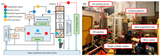
The experimental device was modified based on a single-cylinder engine, and a piston oscillating heat transfer test platform was designed. Figure 1 presents a view of the test setup. The test bench can be mainly divided into four parts: the mechanical motion system, the air heating system, the constant temperature and constant pressure engine oil supply system, and the data acquisition and control system. The test fixture platform is modular and can accommodate different piston tests with cylinder diameters ranging from 100 mm to 150 mm. The air heating system can achieve a maximum air volume of 167.5 m³/h. The data acquisition and control system uses modular hardware and the LabVIEW 2020 software platform, enabling real-time monitoring of multiple sensors, controllers, and actuators.

Figure 1. The piston oscillation cooling comprehensive test bench: (a) test bench schematic (b) visual test bench.

The measurement principle underlying the experimental platform is depicted in Figure 1a. The crankshaft is driven by a motor to achieve reciprocating motion through the connecting rod and the intermediate piston. A heating device is used to heat the air as a high-temperature heat source, simulating high-temperature flue gas. The oil supply system can inject constant-temperature engine oil into the cylinder to cool the piston and lubricate key friction areas. The piston adopts a dual-piston structure, where the guiding piston serves to guide, support, and connect the two connecting rods, meeting the testing requirements for pistons of different cylinder diameters.

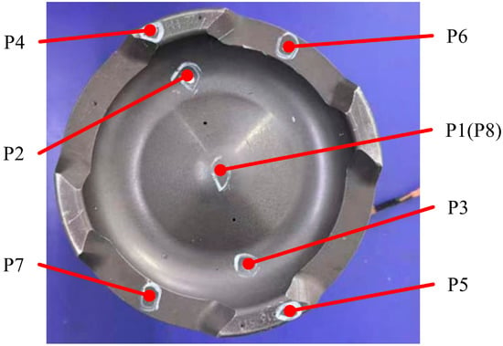
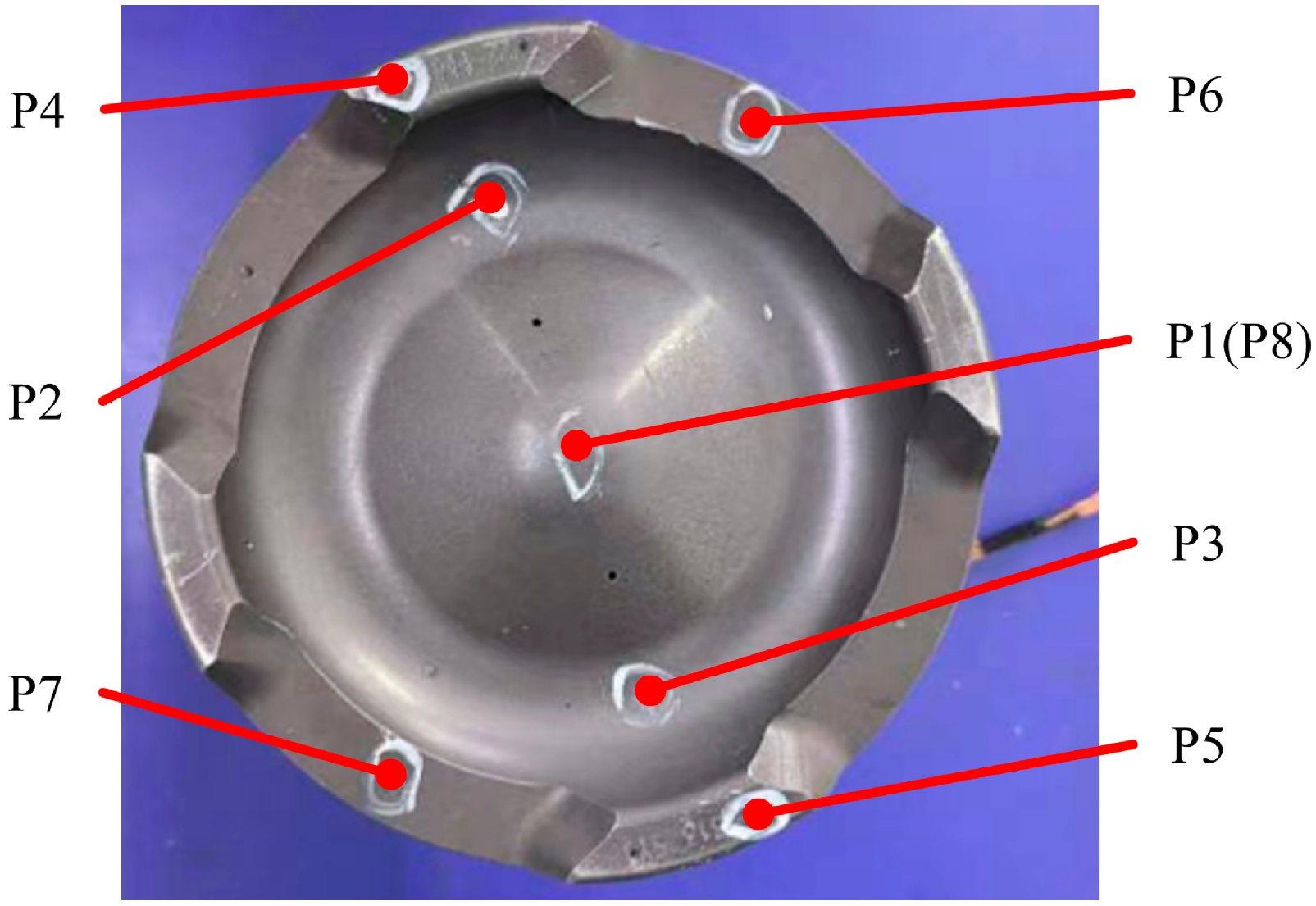
Before testing, thermocouples were installed at eight representative piston locations to resolve the thermal profile on the crown surface and across the associated heat flow routes. Measurement Point 8 was located on the top surface of the piston inner cavity corresponding to Point 1. After the test piston was installed, the air-heating system, oil-supply system, drive system, and data-acquisition system were connected, and the reliability of all connections was checked. Static calibration was performed to ensure measurement stability. During calibration, the piston was positioned at top dead center, and the heater power and fan speed were adjusted until all thermocouple readings reached steady values. This procedure provided a reliable baseline for subsequent validation of the temperature-field simulation. It should be noted that the test rig is mechanically limited to speeds below the neural network training range (1500–2200 rpm). Therefore, these 8 thermocouples served solely to validate the finite element (FE) model, not the neural network. The test bench and thermocouple locations are shown in Figure 2.

Figure 2. Thermocouple arrangement on the piston.

The temperature sensors used are K-type thermocouples with a measurement range of −200 to 500 °C and an accuracy of ±0.5 °C. The thermocouples were fixed at the piston measurement points by welding and further secured with high-temperature adhesive. The temperature acquisition device is a National Instruments NI-9213 module (National Instruments, Austin, TX, USA) with a system accuracy of ±0.1 °C, connected to a computer via USB for real-time monitoring and recording of experimental data. The steady-state condition was defined as the variation in all thermocouple readings being less than ±0.5 °C over a 5-min period.

2.2. Simulation Model Established and Validation

2.2.1. Numerical Method

The research object is an oil jet-cooled aluminum silicon alloy piston, together with its liner and ring pack, from a high-power diesel engine. Because the piston is not fully axisymmetric and the combustion bowl, valve recesses, pin bosses, and internal cooling gallery strongly influence heat-flow distribution, the principal geometric features are retained in the model; only small filets and local chamfers with negligible effects on heat transfer are omitted. The material description is simplified by neglecting the temperature dependence of specific heat, density, elastic modulus, and poisson’s ratio. The material properties are listed in Table 1.

Table 1. Piston material properties.

Temp. (K)	k [W/(m·K)]	α (×10−6/K)	cp [J/(kg·K)]	ρ (kg/m3)	E (GPa)	ν
373	152	21.9	880	2700	70	0.3
473	163	23.9
573	175	24.9

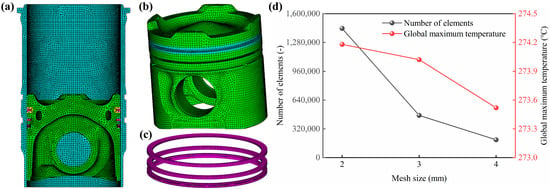
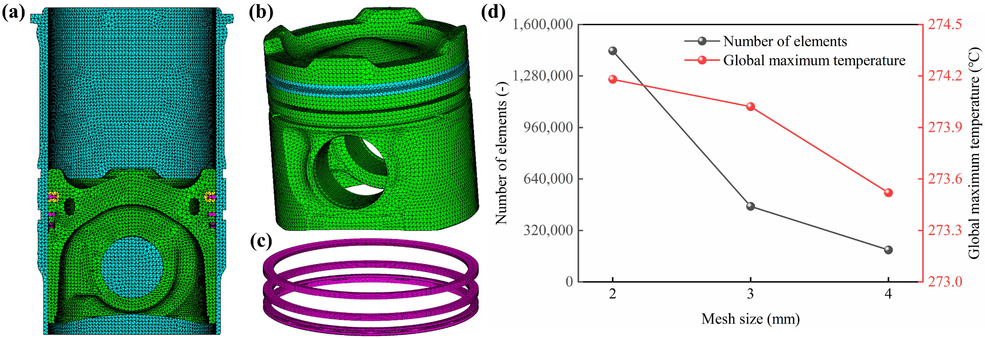
Local refinement was employed in high-gradient regions, including ring grooves, combustion bowl throats, pin bores, and cooling galleries. To determine an appropriate mesh size, a mesh independence study was conducted. Three global mesh sizes were compared: coarse (4 mm), medium (3 mm), and fine (2 mm), all with the same local refinement in high-gradient regions. The global maximum temperature, which occurs at the combustion bowl throat and is most sensitive to mesh resolution, was adopted as the evaluation metric. As shown in Figure 3d, the maximum temperature increases slightly with mesh refinement, and the difference between the medium and fine meshes is only 0.16 °C, confirming that the 3 mm mesh provides sufficient accuracy. Therefore, a global mesh size of 3 mm was adopted for all subsequent simulations to balance computational cost and solution accuracy. The finite element representation of the piston assembly and the cylinder liner, generated using tetrahedral heat-transfer elements (DS6/DC3D10), consisted of 469,457 elements and 606,532 nodes, as shown in Figure 3.

Figure 3. Finite element model and mesh independence analysis: (a) liner; (b) piston; (c) piston ring; (d) variations in the number of elements and the global maximum temperature with mesh size.

2.2.2. Boundary Conditions

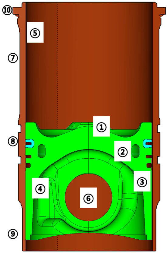
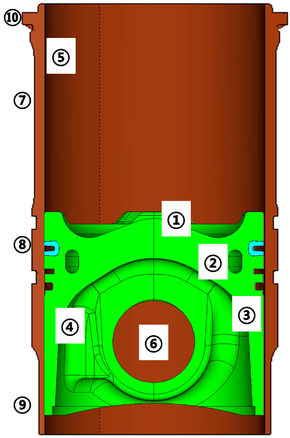
Distinct regions of the piston and the cylinder liner are dominated by different thermal boundary mechanisms [20,21]. The surfaces of both the piston and the cylinder liner are subdivided into multiple heat transfer regions, which aids in the examination of their coupled thermal behavior, and their boundary conditions are determined individually. The thermal boundary loading in different regions is shown in Figure 4. Region 2 is divided into upper gallery wall, outer gallery wall, inner gallery wall and lower gallery wall. Region 4 includes the top of the inner piston cavity, the bottom of the inner piston cavity and pin bore zones. The temperature and heat transfer coefficient of ten regions are listed in Table 2.

Figure 4. Schematic diagram of piston surface.

Table 2. Dynamic thermal boundary conditions for the piston and liner.

Heat-Transfer Region	Temperature (°C)	Heat-Transfer Coefficient [W/(m2·K)]	Region
Piston crown zone	Peak ~1800; Mean 600	Peak ~4400; Mean 760	Region ①
Gas-side inner liner surface			Region ⑤
Upper gallery wall	90	Mean 1081	Region ②
Outer gallery wall	90	Mean 1046	Region ②
Inner gallery wall	90	Mean 926	Region ②
Lower gallery wall	90	Mean 996	Region ②
Top of inner piston cavity	95	1000	Region ④
Bottom of inner piston cavity	95	240	Region ④
Pin bore	95	1000	Region ④
Liner–lubricating-oil side	95	850	Region ⑥
Liner coolant side 1	75	2900	Region ⑦
Liner coolant side 2	75	115	Region ⑧
Liner–engine-block interface 1	600	116	Region ⑩
Liner–engine-block interface 2	95	50	Region ⑨

The detailed methods for determining these thermal boundaries are summarized as follows. For the gas-side boundaries (Regions 1 and 5), the transient gas temperature and heat transfer coefficient were calculated using a one-dimensional thermodynamic cycle simulation coupled with the Woschni correlation, with the spatial distribution on the crown determined by the Seal Taylor correlation. The mean piston crown heat transfer coefficient is 760 W/(m²·K), and the mean gas temperature is 600 °C at the rated condition. For the oscillating cooling boundary (Region 2), a transient CFD model with the VOF method and dynamic meshing was employed. The average convective coefficients along the upper, outer, lower, and inner gallery walls are 1081, 1046, 996, and 926 W/(m²·K), respectively. For the piston side boundaries (Region 4), the heat transfer coefficients of the top land, ring grooves, and oil ring groove were calculated based on thermal contact resistance theory, with values ranging from 239 to 2167 W/(m²·K). For the remaining boundaries, established empirical correlations were adopted, including the Dittus Boelter correlation for the water jacket side.

For the transient calculation, the steady-state temperature distribution is adopted as the initial condition for the unsteady calculation to enhance convergence speed, and the piston is prescribed with an oscillatory motion aligned with the cylinder liner axis. A base time step of 2.725 ms (36 °CA at 2200 r/min) is adopted, with smaller steps at the beginning due to rapid variations in crown temperature and heat-transfer coefficient. The transient simulation was run for 2–3 consecutive engine cycles. The solution was considered periodic and converged when the difference in the maximum piston temperature between consecutive cycles fell below 0.5 °C.

2.2.3. Model Validation

To ensure the reliability of the data source for neural network training, a finite element piston temperature-field model was established under the same steady-state operating and boundary conditions, and the calculated temperatures were compared with the 8 experimental measurements, as listed in Table 3. Across the eight monitoring positions, the experimentally recorded temperatures spanned from 242 °C to 260 °C, while the simulated temperatures ranged from 243 to 265 °C. The two datasets show the same overall trend. The relative error at every point is below 5%; the maximum error, 4.33%, occurs at Point 4. The smaller errors at the remaining points indicate that the model accurately captures the actual piston temperature distribution. Considering calibration and installation errors, the combined experimental uncertainty is estimated to be within ±1.0 °C, which is smaller than the simulation-experiment discrepancy reported in Table 3. It should also be noted that the 8 thermocouple locations, while covering the main heat flow paths, cannot fully represent the entire temperature field, and further experimental validation at additional locations would be beneficial in future work.

Table 3. Comparison of measured and simulated temperatures.

Monitoring Point	Measured Temperature (°C)	Simulated Temperature (°C)	Error
1	249	247	0.80%
2	252	251	0.40%
3	247	250	1.21%
4	254	265	4.33%
5	260	264	1.54%
6	248	257	3.63%
7	256	258	0.78%
8	242	243	0.41%

3. Prediction Model for Temperature Response of Piston Assembly-Cylinder Liner

3.1. Neural Network Structure Selection and Design

The temperature field of the piston assembly cylinder liner system is governed by the coupled effects of multiple factors, including oil temperature, jet velocity, and engine speed, resulting in a complex nonlinear mapping relationship between inputs and outputs. The problem addressed in this study is a regression problem, and the goal of network training is to continuously correct the weights and biases of each layer of neurons through iterative optimization, in order to minimize the error between predicted values and true values [22,23].

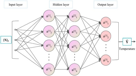
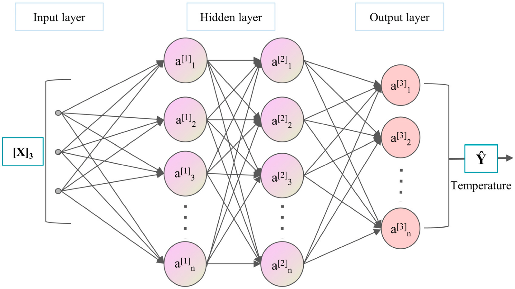
This study uses a fully connected feedforward deep neural network, whose basic structure is shown in Figure 5. The network consists of three parts: input layer, hidden layer, and output layer. The input layer is responsible for receiving external data, the hidden layer extracts high-order nonlinear information from the input features through a hierarchical transformation of multiple layers of neurons, and the output layer maps the calculation results of the hidden layer to the final predicted value. Each layer of neurons receives the output of the previous layer, and after weighted summation, bias superposition, and non-linear transformation of the activation function, it is transmitted to the next layer. This process is called forward propagation.

Figure 5. Neural network structure diagram.

In determining the number of hidden layers and neurons, a trial and error comparison method was used. Taking root mean square error (RMSE) and coefficient of determination (R²) as evaluation indicators, and considering the fitting accuracy and generalization ability, the network structure is finally determined as follows: the input layer contains three neurons, corresponding to three input variables: oil temperature, jet velocity, and rotational speed. The hidden layer consists of 3 layers, with 32, 16, and 8 neurons respectively. It adopts a structure design that decreases layer by layer, which is conducive to extracting hierarchical information from input features. The activation function adopts ReLU, which has the advantages of simple calculation and alleviating gradient vanishing. The output layer contains one neuron and uses a linear activation function to output the temperature prediction values of the corresponding feature points. It should be noted that 18 separate single-output networks were trained, one for each characteristic point. Each network adopts the same architecture and hyperparameters but has a single output neuron corresponding to the temperature at its assigned point. The summary of network structure parameters is shown in Table 4. It should be acknowledged that, as the primary focus of this study is to propose a methodological framework, the selection of the 32-16-8 architecture and λ = 0.1 was based on preliminary trials and engineering judgment rather than a systematic sensitivity analysis. A systematic sensitivity analysis regarding the dataset size, network architecture, and weighting parameters will be addressed in future work.

Table 4. Neural network structure parameters.

Structure/Parameters	Value
Input layer variables	Oil temperature, jet velocity, and rotational speed
Output layer variables	Temperature of each characteristic point
Hidden layer structure	3 layers (32-16-8 neurons)
Hidden layer activation function	ReLU
Loss Function	MSE+physical constraint loss
Optimizer	Adam
λ	0.1

The loss function consists of two parts: a data-driven term and a physical constraint term [24]. The data-driven term uses mean square error (MSE) to measure the deviation between predicted values and true values. The physical constraint term is based on prior knowledge discovered in the influence law of a single factor, and the partial derivatives of the network output on the speed and oil temperature are automatically differentiated. The ReLU function is used to penalize gradient predictions that violate monotonicity direction. The total loss function is

$$L_{\mathrm{tol}}=L_{\mathrm{MSE}}+L_{\mathrm{phy}}={\displaystyle \frac{1}{N}}\sum _{i=1}^N{({\widehat{T}}_i-T_i)}^2+\lambda {\displaystyle \frac{1}{N}}\sum _{i=1}^N[\mathrm{ReLU}(-{\displaystyle \frac{\partial {\widehat{T}}_i}{\partial n_i}})+\mathrm{ReLU}(-{\displaystyle \frac{\partial {\widehat{T}}_i}{\partial t_i}})]$$

(1)

where the first term is the mean square error term, the second term is the physical constraint term. ${\widehat{T}}_i$ is the predicted temperature, while n_i and t_i are the standardized engine speed and oil temperature. Based on the physical trends in Section 4.1, temperature increases monotonically with speed and oil temperature, so the expected derivatives are $\partial {\widehat{\mathrm{T}}}_{\mathrm{i}}/\partial {\mathrm{n}}_{\mathrm{i}}>0$ and $\partial {\widehat{\mathrm{T}}}_{\mathrm{i}}/\partial t_{\mathrm{i}}>0$. The ReLU terms penalize negative derivatives that violate this monotonicity. Since standardization is a linear monotonic transformation, the derivative sign is preserved, ensuring the validity of the constraint. The optimizer uses the Adam algorithm with an initial learning rate of 0.001.

3.2. Sample Point Design

In order to train and test neural network models, representative sample points need to be selected in the input parameter space. This study selected oil temperature t ∈ [60, 100] °C, jet velocity v ∈ [9, 21] m/s, and engine speed n ∈ {1500, 1900, 2200} r/min forms the sample space. The Latin hypercube design method was used to sample the (t, v) two-dimensional sample space at each speed condition. This method divides the value range of each input parameter into m non overlapping intervals, randomly selects a value in each interval, and then randomly matches the selected values of each parameter to form m sample points. The Latin hypercube design ensures that the one-dimensional projection of each parameter was uniformly covered with a limited sample size, while achieving good filling of multidimensional space through random combinations.

Based on the above method, 20 sample points were generated for each speed condition, totaling 60 sample points for three speeds. The 20 sample points can form a relatively uniform coverage in two-dimensional space, with each dimension equivalent to dividing the interval into 20 segments, each represented by a sample, while effectively controlling computational costs. Rounding the generated sample points appropriately ensures the engineering usability of the parameter values. The specific parameter values for 20 sample points under each speed condition are shown in Table 5.

Table 5. Latin hypercube design sample point parameter.

Condition	Oil Temperature (°C)	Jet Velocity (m/s)	Condition	Oil Temperature (°C)	Jet Velocity (m/s)
1	73	13.5	11	61	17.7
2	95	18.3	12	99	14.1
3	63	10.5	13	93	11.1
4	79	15.3	14	77	9.9
5	89	18.9	15	97	16.5
6	87	20.1	16	67	12.9
7	75	19.5	17	65	11.7
8	69	17.1	18	85	15.9
9	83	14.7	19	81	12.3
10	91	20.7	20	71	9.3

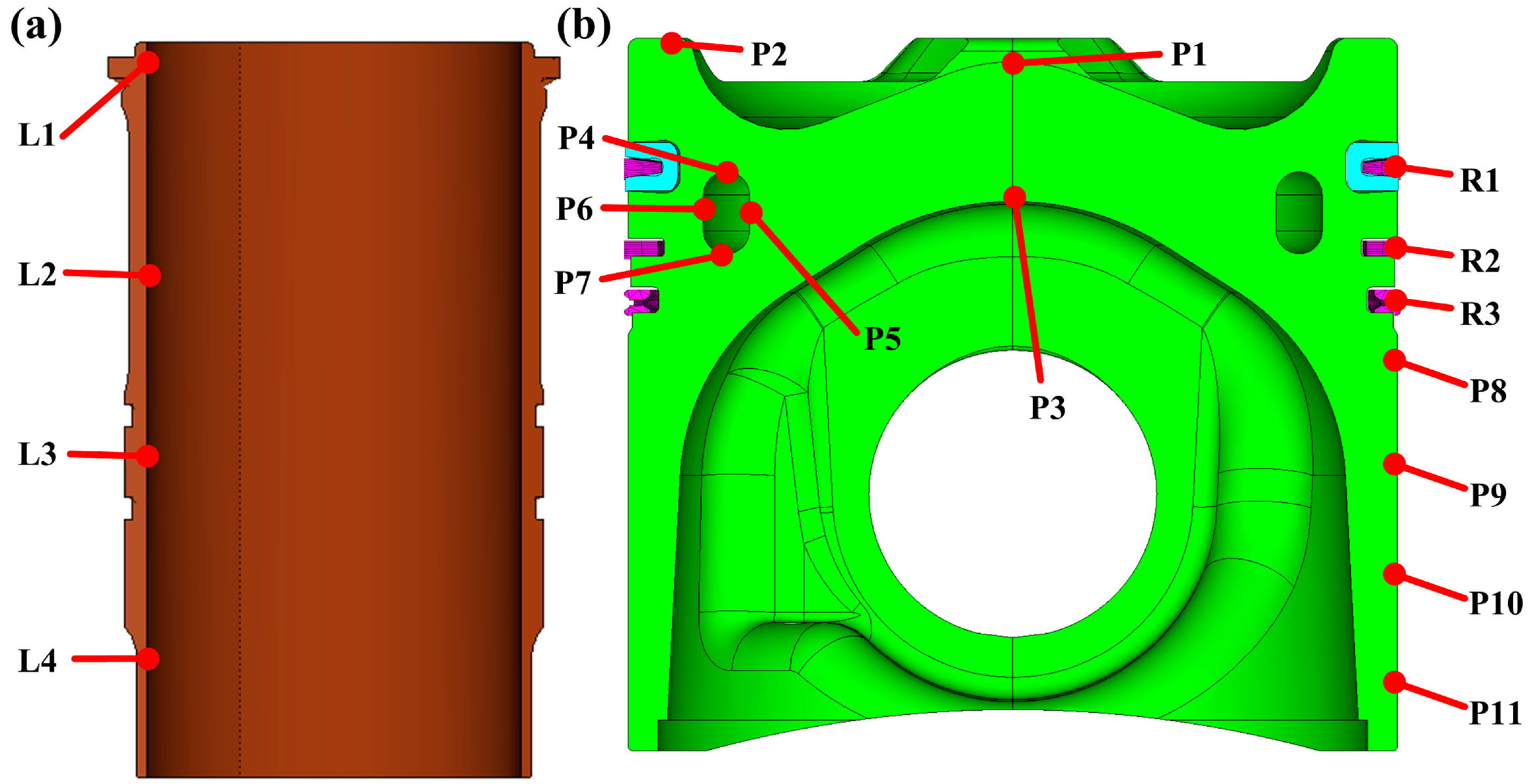
For each set of sample points, based on the calibrated piston cylinder liner fluid solid thermal coupling simulation model, the piston temperature field was calculated using the oil temperature, jet velocity, and rotational speed as input conditions, and the temperature of each feature point was extracted as the output response. The simulation results of all 60 sample points constitute the basic dataset for neural network modeling. Following the validation of the FE model, 18 characteristic points were extracted from the simulations to construct the neural network dataset. These points are virtual extraction locations and do not spatially correspond to the 8 experimental thermocouples. The distribution positions of each feature point are shown in Figure 6, where P1~P11 are the measuring points of the piston body, covering the top of the piston, the walls of the internal cooling oil chamber, and the skirt; R1~R3 are measuring points in the ring area; L1~L4 are the longitudinal measuring points of the cylinder liner.

3.3. Model Training and Validation

The model training and testing data are entirely based on the simulation results of Latin hypercube design sampling points. The 60 simulation cases are divided into a training set (80%, 48 cases) and a validation set (20%, 12 cases) using a stratified split by engine speed, ensuring each speed condition (1500, 1900, 2200 r/min) contributes an equal proportion to both subsets. The split was performed once with a fixed random seed to ensure reproducibility. The training set is used for parameter learning, while the validation set is used for hyperparameter tuning and monitoring convergence. The final evaluation is performed on a separate independent test set. It should be emphasized that the validation in this study follows a two-step hierarchy: firstly, the finite element model is validated against experiments; secondly, the neural network is validated against the finite element simulation data. To eliminate the influence of dimensional differences between input and output variables on the training process, the input and output variables are standardized and transformed into a standard normal distribution with a mean of 0 and a standard deviation of 1. The standardized formula is

$$x_{\mathrm{scaled}}={\displaystyle \frac{\left(x-{\mu }_{\mathrm{x}}\right)}{{\sigma }_{\mathrm{x}}}}$$

(2)

Figure 6. Location of characteristic points of piston assembly cylinder liner: (a) liner; (b) pistons and piston rings.

Figure 6. Location of characteristic points of piston assembly cylinder liner: (a) liner; (b) pistons and piston rings.

In the formula, μ_x and σ_x represent the mean and standard deviation of the corresponding variables in the training set. After the model training is completed and forward propagation prediction is performed, the saved mean and standard deviation are restored to their original dimensions through inverse transformation.

On the basis of the above deep neural network structure, the RMSE and coefficient of determination R² are used as evaluation indicators for model accuracy. The calculation formula is as follows:

$$\mathrm{RMSE}=\sqrt{{\displaystyle \frac{1}{N}}\sum _{i=1}^n{\left({\widehat{T}}_i-T_i\right)}^2}$$

(3)

$${\mathrm{R}}^2=1-{\displaystyle \frac{{\sum }_{i=1}^n{\left(T_i-{\widehat{T}}_i\right)}^2}{{\sum }_{i=1}^n{\left(T_i-\overline{T}\right)}^2}}$$

(4)

The standardized training data were encapsulated into PyTorch (version 2.8.0) tensors, and batch loads were constructed using DataLoader. The training details are summarized as follows: the random seed was set to 1 for both PyTorch and NumPy (version 1.23.5); the batch size was 4 for training and 2 for validation; the maximum number of epochs was 2000; the optimizer was Adam with an initial learning rate of 0.001 and a weight decay of 1 × 10⁻³. The model was trained for a fixed 2000 epochs, and the loss curves on the training and validation sets were monitored to confirm convergence without overfitting. To evaluate the benefit of the physical constraint, a comparative study was conducted between the physics-constrained neural network (λ = 0.1) and an unconstrained neural network (λ = 0) using identical network architecture, training data, and test set.

4. Results and Discussion

4.1. The Influence of Boundary Parameters on Heat Transfer Characteristics

4.1.1. The Influence of Engine Speed

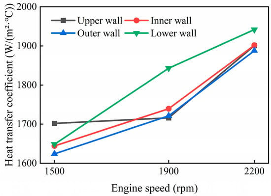
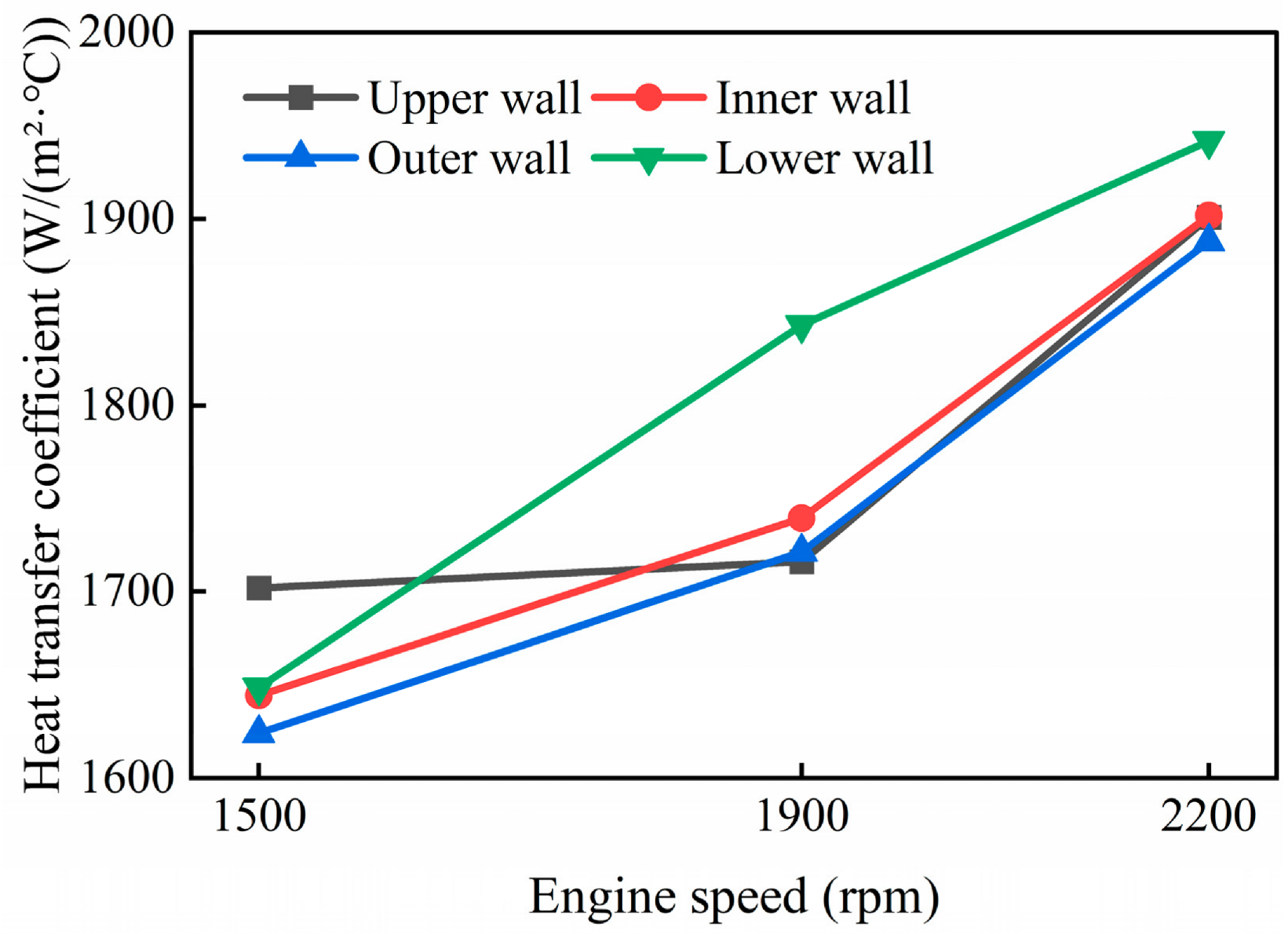
Maintain oil temperature at 80 °C and jet velocity at 15 m/s. Choose three speeds of 1500 r/min, 1900 r/min, and 2200 r/min to compare the heat transfer characteristics of the piston cylinder liner system. Figure 7 shows the average heat transfer coefficient of each wall surface of the internal cooling gallery inside the piston at different speeds. As the speed increases from 1500 r/min to 2200 r/min, the heat transfer coefficients of each wall surface show an upward trend, but the increases vary among the walls. The lower wall exhibits the largest increase of 17.8%, while the upper wall shows the smallest increase of 11.2%. This is mainly related to the degree of oil coverage and impact strength on different wall surfaces. In addition, at high speeds, the heat transfer coefficients of each wall tend to be uniform, indicating that the oil oscillation in the oil chamber is more severe and the distribution is more uniform.

Figure 7. Heat transfer coefficient of the internal cooling gallery wall inside the piston at different speeds.

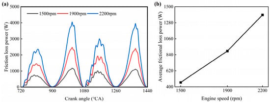
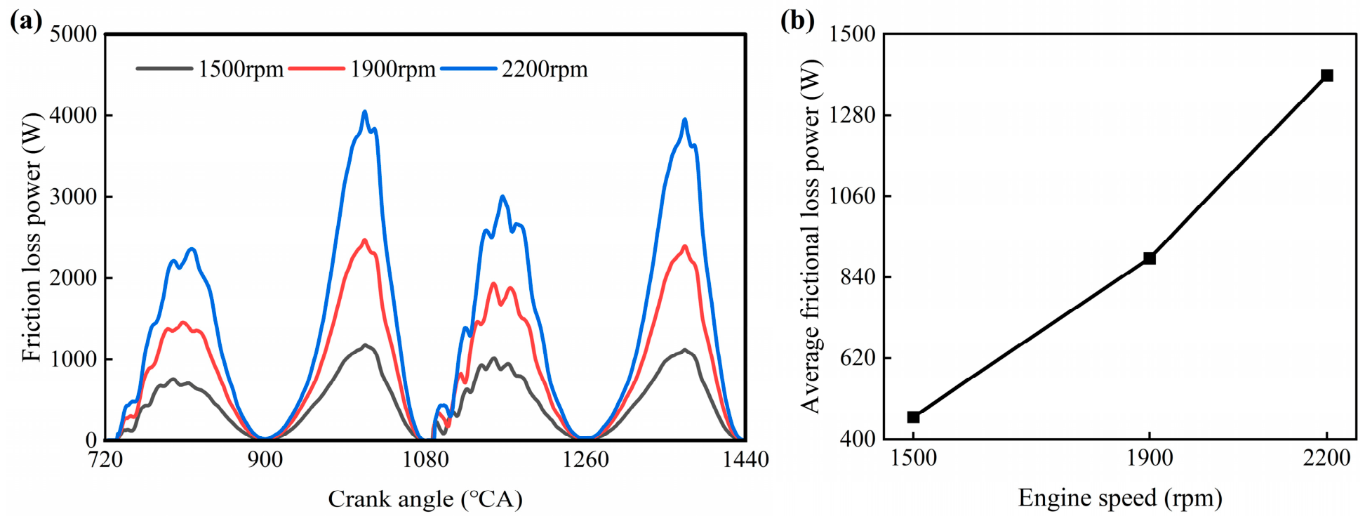
Figure 8 shows the variation in frictional loss power between skirt cylinder liner and ring cylinder liner at different speeds. The frictional loss power of the skirt increases significantly with the increase in rotational speed, and the global peak value increases from 1177.4 W at 1500 r/min to 4051.6 W at 2200 r/min, with an increase of about 244%. The average frictional loss power increased from 460.4 W to 1389.2 W, an increase of about 202%. The main reason for the significant increase in frictional loss with rotational speed is that the increase in piston movement speed leads to an increase in the shear rate of the lubricating oil film. At the same time, the increase in cylinder gas pressure at high speeds increases the contact load between the ring group and the cylinder sleeve, which together exacerbate frictional loss.

Figure 8. Friction loss of skirt at different rotational speeds: (a) friction loss power variation curve; (b) average frictional loss power.

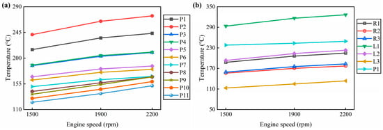
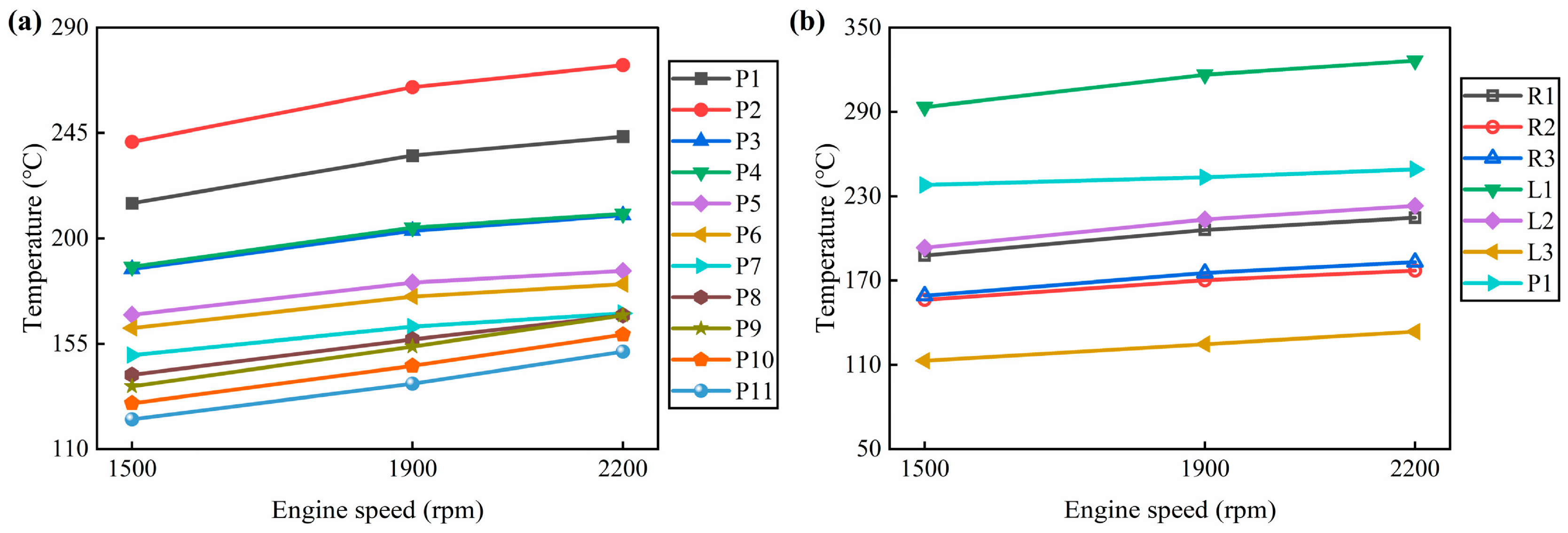
Based on the changes in the thermal boundary conditions mentioned above, Figure 9 shows the effect of rotational speed on the temperature of each characteristic point. The center P1 at the top of the piston increased from 215.1 °C to 243.5 °C, the highest temperature point P2 increased from 241.2 °C to 274.0 °C, and the upper L1 of the cylinder liner increased from 293.5 °C to 326.5 °C. The combustion bowl throat region consistently exhibited the highest temperature across all speeds due to its direct exposure to high-temperature combustion gases and limited cooling access. Among the measuring points, the temperature level was the highest, while the temperature rise at the bottom L4 of the cylinder liner was relatively mild. The temperature rises as the rotational speed increases, with the areas directly affected by the gas, namely the top of the piston and the upper part of the cylinder liner, experiencing the most significant temperature rise. Based on the changes in the heat transfer coefficient mentioned above, it can be concluded that the increase in rotational speed enhances the temperature level of the system through two paths: gas side convection and oil chamber oscillation heat transfer. The differences in temperature rise amplitude at different locations reflect the different dominant heat transfer paths in each region.

Figure 9. Temperature of characteristic points of piston assembly cylinder liner at different speeds: (a) piston; (b) rings and liner.

4.1.2. The Influence of Oil Temperature

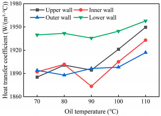
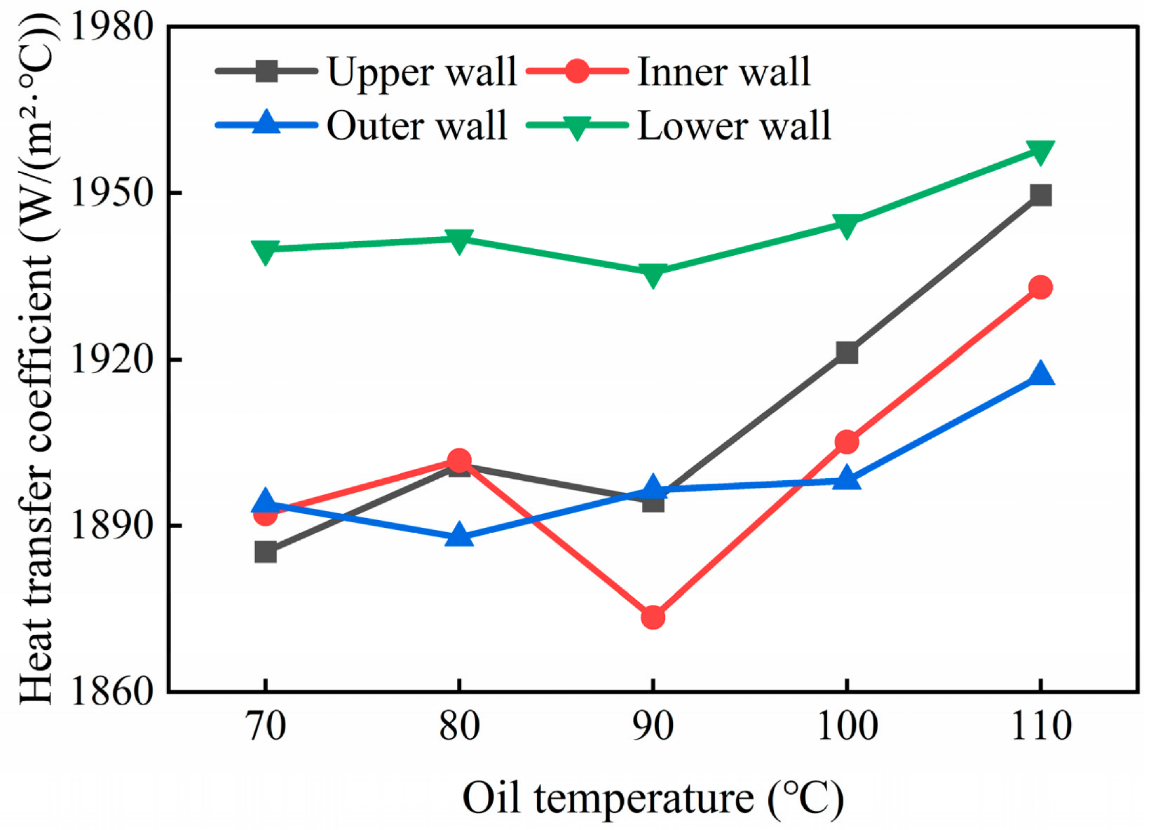
Maintain a speed of 2200 r/min and a jet velocity of 15 m/s. Select four oil temperatures of 70 °C, 80 °C, 90 °C, and 100 °C to compare and analyze the heat transfer characteristics of the piston cylinder liner system. Figure 10 shows the average heat transfer coefficient of each wall surface of the internal cooling gallery inside the piston at different oil temperatures. As the oil temperature rises from 70 °C to 100 °C, the trend of heat transfer coefficients on each wall varies. The heat transfer coefficient of the upper wall increased from 1885.3 W/(m²·K) to 1949.6 W/(m²·K), an increase of about 3.4%; the lower wall increased from 1939.8 W/(m²·K) to 1957.8 W/(m²·K), with an increase of only about 0.9%; and the inner and outer walls exhibited a fluctuating characteristic of first rising, then falling, and then rising again. This indicates that the increase in oil temperature has the most sustained heat transfer enhancement effect on the upper wall surface, with a weak impact on the lower wall surface, while the inner and outer wall surfaces exhibit non monotonic changes due to the combined effects of viscosity and flow state.

Figure 10. Heat transfer coefficient of the internal cooling gallery wall inside the piston at different oil temperatures.

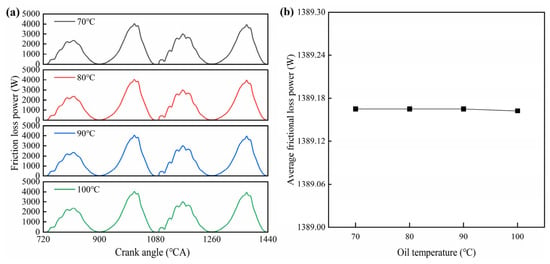
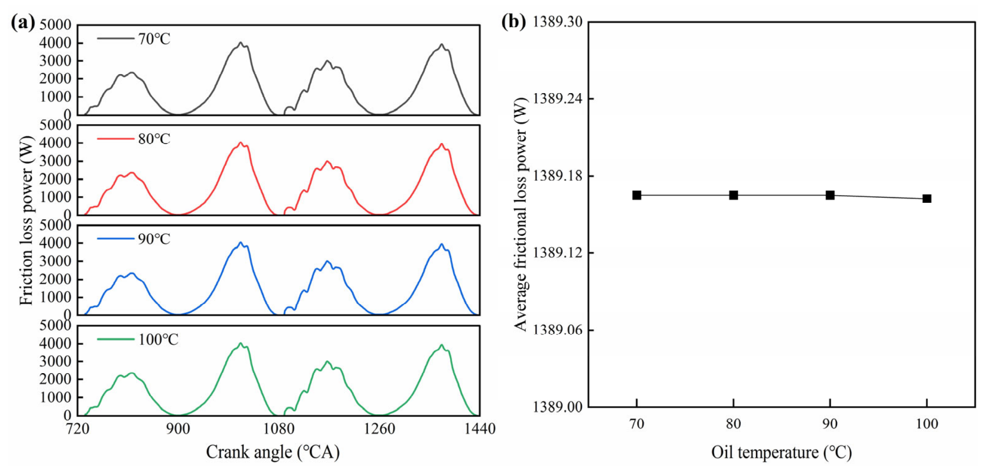
Figure 11 shows the variation in work loss due to skirt-cylinder liner friction at different oil temperatures. The curves of friction loss work with crankshaft angle at four different oil temperatures almost completely overlap, and the global peak and average values remain consistent, indicating that within the oil temperature range from 70 °C to 100 °C investigated in this study, the influence of oil temperature changes on skirt friction loss work is minimal. The reason is that although the viscosity of the oil decreases with increasing temperature, the friction state between the skirt and cylinder liner is mainly dominated by the piston movement speed and gas pressure load, and the shear force difference caused by changes in oil viscosity accounts for a relatively small proportion of the total friction loss.

Figure 11. Friction loss of skirt at different oil temperatures: (a) friction loss power variation curves; (b) average frictional loss power.

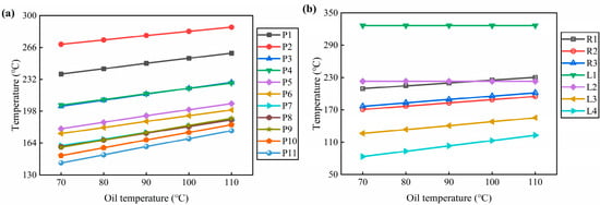
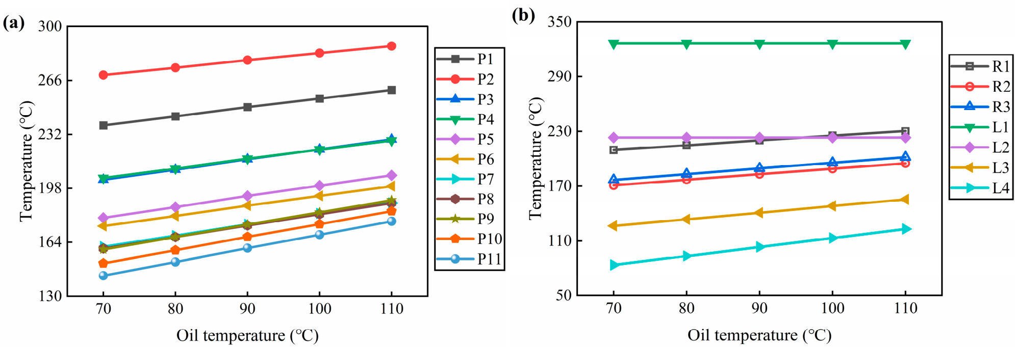
Based on the changes in the thermal boundary conditions mentioned above, Figure 12 shows the influence of oil temperature on each characteristic point. The center P1 of the piston top increased from 237.9 °C to 260.2 °C, and the top P3 of the inner cavity increased from 203.5 °C to 228.8 °C, an increase of about 12.4%. The temperature of each wall in the internal cooling oil chamber also increases with oil temperature, with the largest increase observed at P7 on the lower wall, approximately 17.2%. The end of the skirt P11 increased from 143.1 °C to 177.1 °C, an increase of about 23.8%, showing the most significant response among the piston body measuring points. The temperature of L1 at the upper part of the cylinder liner remains unchanged at 326.5 °C, while L4 at the bottom of the cylinder liner increases from 83.4 °C to 123.1 °C, an increase of about 47.6%. The overall increase in oil temperature has raised the temperature levels of the piston body and the lower part of the cylinder liner, but the impact on different parts varies significantly. The upper part of the cylinder liner is mainly dominated by heat flow from the gas side and is not sensitive to oil temperature changes. The temperature of the lower part of the cylinder liner and the piston skirt, which are close to the cooling medium and far away from the combustion chamber, increases significantly with the rise in oil temperature.

Figure 12. Temperature of characteristic points of piston assembly cylinder liner at different oil temperatures: (a) piston; (b) rings and liner.

4.1.3. The Influence of Oil Jet Velocity

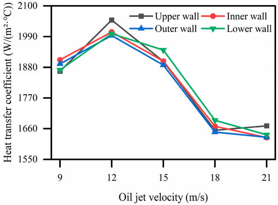
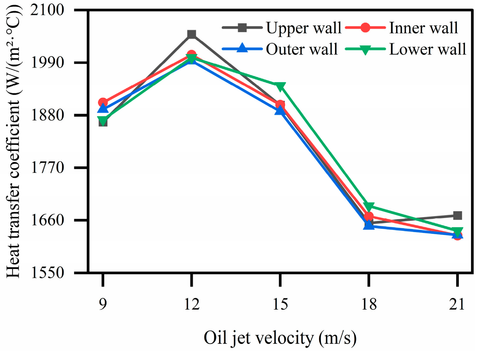
Maintain a speed of 2200 r/min and an oil temperature of 80 °C. Select five jet velocities of 9 m/s, 12 m/s, 15 m/s, 18 m/s, and 21 m/s to compare and analyze the heat transfer characteristics of the piston cylinder liner system. Figure 13 shows the average heat transfer coefficient of each wall surface of the internal cooling gallery inside the piston at different jet velocities. As the jet velocity increases from 9 m/s to 12 m/s, the heat transfer coefficients of each wall significantly increase, with the upper wall, inner wall, outer wall, and lower wall increasing by 9.8%, 5.3%, 5.4%, and 7.0%, respectively, with the upper wall being the most sensitive in response. When the jet velocity further increases to 15 m/s, the heat transfer coefficient drops significantly compared to 12 m/s, with a decrease of 7.2% on the upper wall surface. After the jet velocity exceeds 15 m/s, the heat transfer coefficients of each wall continue to decrease and tend to flatten out. This indicates that the heat transfer coefficient of the internal cooling oil chamber does not increase monotonically with the jet velocity, but there exists an optimal jet velocity around 12 m/s under this operating condition. Beyond this optimal velocity, the heat transfer performance is weakened by several combined mechanisms. The shortened residence time of the oil in the cooling gallery reduces the time available for heat absorption. Meanwhile, the high-velocity jet tends to cause uneven oil distribution and local dry-out on the gallery walls, and the oil film may break up under strong shear forces, reducing the effective contact area for heat transfer. These factors may collectively lead to the observed reduction in heat transfer coefficient at high jet velocities, which requires further experimental and numerical verification.

Figure 13. Heat transfer coefficient of the internal cooling gallery wall inside the piston at different oil jet velocities.

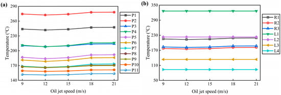
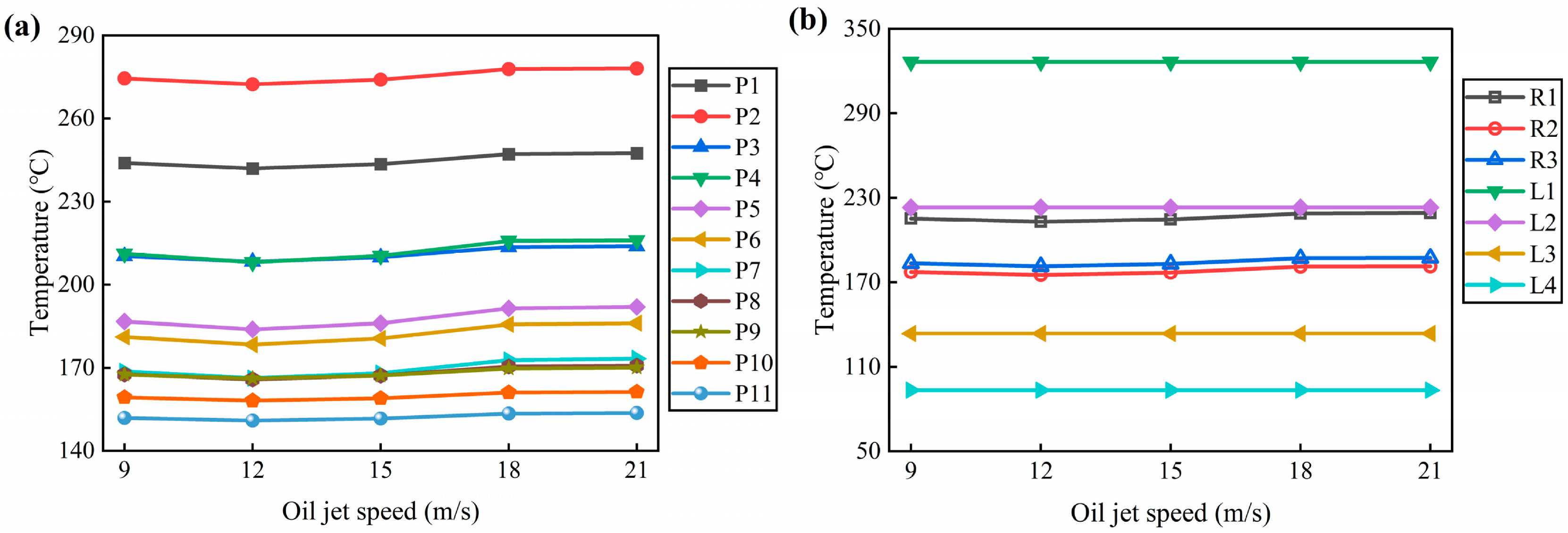
Based on the changes in the thermal boundary conditions mentioned above, Figure 14 shows the influence of jet velocity on the temperature of each characteristic point. The temperature at each measuring point drops to its lowest point when the jet velocity is about 12 m/s, and then rises with the increase in jet velocity, but the overall change amplitude is relatively small. The center P1 of the piston top drops to 242.0 °C at 12 m/s, a decrease of about 0.8% compared to 9 m/s, and then rises to 247.4 °C at 21 m/s. The measuring points on the walls and ring area of the internal cooling oil chamber show the same trend, with the lowest temperature at 12 m/s. The measuring points of the cylinder liner remain basically unchanged at different jet velocities. The temperature change caused by jet velocity is significantly smaller than the effects of rotational speed and oil temperature. The reason is that jet velocity only acts on a local area of the internal cooling oil chamber, and the heat transfer to areas far away from the oil chamber has been greatly attenuated. Moreover, the oil flow within the range of 9–21 m/s is already in a fully turbulent zone, and the sensitivity of the heat transfer coefficient to flow velocity changes is relatively low. Therefore, jet velocity can be used as an auxiliary control means, but its adjustment range is limited.

Figure 14. Temperature of characteristic points of piston assembly cylinder liner at different oil jet velocities: (a) piston; (b) rings and liner.

4.2. The Prediction Results of Neural Networks

To comprehensively evaluate the predictive ability of the constructed neural network model in various parts of the piston assembly cylinder liner system, independent neural network models were established for all 18 characteristic points for training and testing. Each model adopts the same network structure and hyperparameter settings, with speed, oil temperature, and jet velocity as inputs, and temperature values of corresponding feature points as outputs.

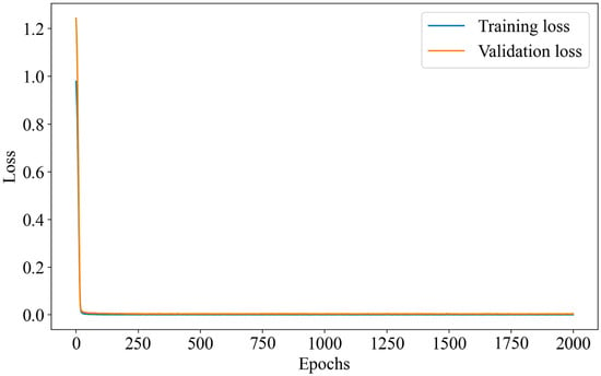
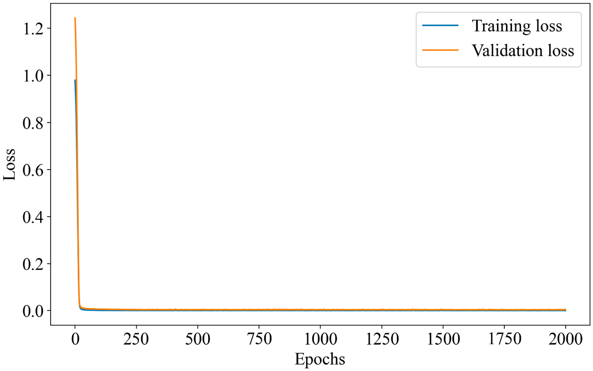
Taking the center measurement point P1 at the top of the piston as an example, the loss variation curves on the training and validation sets during the training process are shown in Figure 15. As can be seen, with the increase in training epochs, both training loss and validation loss show a stable downward trend, and tend to converge after about 300 epochs, without obvious overfitting phenomenon, indicating that the model training process is stable and effective.

Figure 15. Training and validation loss curves for the P1 temperature prediction model.

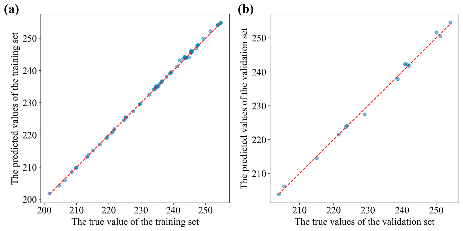
Quantitatively evaluate the prediction accuracy of all 18 characteristic points. Figure 16 shows the scatter comparison between the predicted values of the P1 measurement point neural network and the simulated values. The data points are closely distributed around the diagonal, indicating that the predicted values of the measurement point are highly consistent with the true values. The prediction accuracy of the remaining 17 characteristic points is comparable. On the training and validation sets, R² values are above 0.995 and RMSE values are below 1.0 °C for all 18 characteristic points. Among them, L3 of the cylinder liner achieves the highest accuracy with an R² of 0.9999 and RMSE of 0.15 °C, while R3 of the oil ring yields the lowest accuracy with an R² of 0.9952 and RMSE of 0.93 °C. The above results show that the constructed neural network model maintains good fitting accuracy on the training and validation data at the characteristic points with different heat transfer characteristics and different spatial positions.

Figure 16. Comparison between neural-network-predicted and simulated temperatures for point P1: (a) training set; (b) validation set.

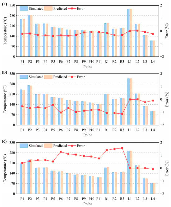
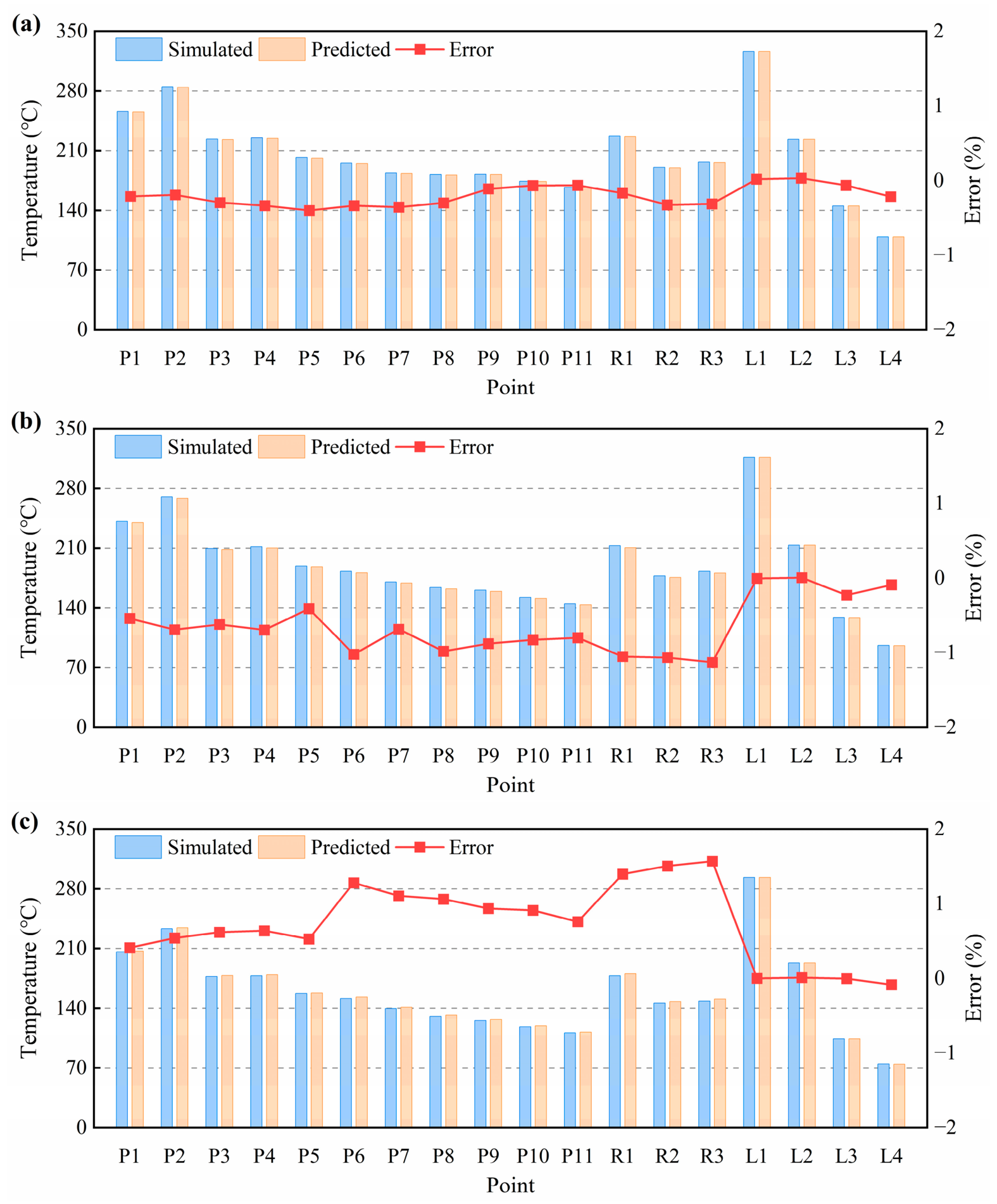
To verify the generalization ability of the model under untrained conditions, three independent sample points that did not participate in training were randomly selected in the sample space for prediction accuracy validation. These three cases constitute the independent test set and are used only for the final evaluation of the model. The parameters of each condition are shown in Table 6, and the comparison between the predicted and simulated temperatures for all 18 characteristic points is presented in Figure 17.

Table 6. Test case.

Condition	Oil Temperature (°C)	Jet Velocity (m/s)	Speed (r/min)
1	96	19.2	2200
2	86	17.5	1900
3	68	14.3	1500

Figure 17. Comparison of simulated and neural-network-predicted temperatures at 18 characteristic points under the three independent test conditions: (a) condition 1; (b) condition 2; (c) condition 3.

The prediction accuracy of the model on the independent test set is quantitatively evaluated using R² and RMSE, as listed in Table 7. All 18 characteristic points achieve R² values above 0.995 and RMSE values below 1.0 °C, confirming the good interpolation capability of the model within the investigated parameter space. Among them, L1 of the cylinder liner achieves the highest accuracy, while R1 of the top ring yields the lowest. The relative prediction errors of the 18 characteristic points under the three conditions are all at a low level, with the maximum relative error of all test predictions within ±1.6%. In the measurement points of the piston body, the prediction error of the highest temperature region P2 is between −0.69% and 0.54%, indicating high accuracy. The error of the measuring points in the ring area is slightly higher than that of the piston body. The error of R3 under working condition three is 1.57%, which is the largest among all measuring points. This may be related to the coupling effect of multiple factors on the temperature in the ring area and the more complex response law. The cylinder liner measuring point errors are all close to zero. All three operating conditions maintained good interpolation accuracy in the training sample space. However, due to the mechanical limitations of the test rig, the experimental speed could not cover the full training range. Therefore, direct experimental validation of the neural network under high-speed conditions is not feasible in this study. Nevertheless, the high accuracy of the neural network within the simulation space, combined with the experimentally validated finite element model, provides a reliable tool for rapid prediction within the investigated range. Expanding the experimental database will be the focus of future work.

Table 7. Prediction accuracy of the neural network on the independent test set.

Characteristic Points	R2	RMSE (°C)	Characteristic Points	R2	RMSE (°C)
P1	0.9979	0.95	P10	0.9999	0.12
P2	0.9993	0.55	P11	0.9999	0.10
P3	0.9996	0.35	R1	0.9971	0.70
P4	0.9996	0.33	R2	0.9989	0.43
P5	0.9998	0.24	R3	0.9979	0.47
P6	0.9991	0.57	L1	1.0000	0.05
P7	0.9997	0.31	L2	1.0000	0.01
P8	0.9993	0.46	L3	0.9999	0.03
P9	0.9999	0.13	L4	0.9998	0.06

Regarding computational efficiency, the entire numerical simulation process, including the transient thermal boundary calculations and finite element solution, is computationally expensive and time-consuming. Once trained, the neural network can predict the temperatures at all 18 characteristic points within 2–3 s, making it highly suitable for rapid thermal assessment and iterative optimization tasks.

To further demonstrate the benefit of the physical constraint, Table 8 compares the prediction performance of the physics-constrained NN (λ = 0.1) and the unconstrained NN (λ = 0) on the independent test set. Within the investigated dataset and test configuration, the physics-constrained NN reduces the overall average test RMSE by 9.5% and slightly improves the average test R². This demonstrates that the physical constraint effectively improves the model’s generalization capability without compromising its fitting ability.

Table 8. Comparison of the overall prediction performance between the physics-constrained NN (λ = 0.1) and the unconstrained NN (λ = 0) on the independent test set.

Model	Average Test RMSE (°C)	Average Test R2
Unconstrained NN	0.924	0.9978
Physics-constrained NN	0.836	0.9981

5. Conclusions

This article establishes a dynamic heat transfer model for the piston assembly-cylinder liner system, and verifies the effectiveness of the model through temperature field experiments. On this basis, the influence of rotational speed, oil temperature, and jet velocity on the heat transfer characteristics and temperature field of the piston cylinder liner system was explored, and a fast prediction model for piston temperature field based on physical constraints and deep neural network was constructed. The main conclusions are as follows:

(1)

The dynamic heat transfer model of the piston assembly-cylinder liner established has good agreement between the predicted temperature and the experimental measurement values, with relative errors of less than 5% at each monitoring point, a maximum error of 4.33%, and an average error of about 1.64%, verifying the accuracy of the model in characterizing the actual temperature distribution of the piston.

(2)

An increase in rotational speed can enhance the heat transfer capacity of various wall surfaces in the internal cooling oil chamber and significantly increase the frictional loss work. The influence of jet velocity on the heat transfer coefficient has an optimal value, and excessively high flow velocity can actually weaken the heat transfer effect; The oil temperature has no significant effect on the frictional loss of the skirt.

(3)

The overall increase in speed and oil temperature raises the temperature level of the piston cylinder liner system, with the most significant response in the area directly affected by gas. The adjustment range of jet velocity on the temperature of various parts is limited.

(4)

The physical constrained deep neural network model constructed has good prediction accuracy for the temperature of 18 characteristic points, with R² above 0.995 and the maximum relative error of all test predictions within ±1.6% within the investigated simulation parameter space. The model exhibits good interpolation capability and can achieve rapid prediction of the temperature at characteristic points of the piston assembly-cylinder liner system. Further experimental validation under a wider range of operating conditions is required to fully establish its extrapolation capability.

References

- Ravikumar, A.; Wright, S.; Redmond, L.; Gingrich, E.; Korivi, V.; Tess, M.; Piehl, J.; Lawler, B. Numerical Evaluation of Injection Parameters on Transient Heat Flux and Temperature Distribution of a Heavy-Duty Diesel Engine Piston. In WCX SAE World Congress Experience; SAE Technical Paper; SAE International: Detroit, MI, USA, 2024. [Google Scholar] [CrossRef] [Scilit]
- Jiang, B.; Qian, Z.; Wang, C.; Fei, C.; Zhu, S.; Shu, Z.; Du, Y.; Wang, X. Simulation Analysis of La2Ce2O7 Thermal Barrier Coating in Marine Internal Combustion Engine. Case Stud. Therm. Eng. 2024, 64, 105564. [Google Scholar] [CrossRef] [Scilit]
- Climent, H.; Tiseira, A.; Gomez-Soriano, J.; Darbhamalla, A. In-Cylinder Heat Transfer Model Proposal Compatible with 1D Simulations in Uniflow Scavenged Engines. Appl. Sci. 2023, 13, 3996. [Google Scholar] [CrossRef] [Scilit]
- Broatch, A.; Olmeda, P.; Margot, X.; Escalona, J.L. Conjugate Heat Transfer Study of the Impact of ‘Thermo-Swing’ Coatings on Internal Combustion Engines Heat Losses. Int. J. Engine Res. 2020, 22, 2958–2967. [Google Scholar] [CrossRef] [Scilit]
- Chen, Y.; Schlautman, J.; Dhar, S. Experimental and Numerical Investigation of the Multiphase Flow and Heat Transfer in an Oil Jet Cooled Engine Piston. In WCX SAE World Congress Experience; SAE Technical Paper; SAE International: Detroit, MI, USA, 2020. [Google Scholar] [CrossRef] [Scilit]
- Sahu, A.K.; Chakkamadathil, S.; Das, D. Integrated Simulation Methodology to Predict Engine Head, Block, and Piston Temperatures. In Symposium on International Automotive Technology; SAE Technical Paper; SAE International: Detroit, MI, USA, 2023. [Google Scholar] [CrossRef] [Scilit]
- Fan, Z.; Wang, G.; Yu, Q.; Chen, G.; Niu, X.; Wang, Y. Numerical and Experimental Study of Heat Transfer Characteristics of Piston Combustion Chamber Wall in Marine High Power Density Engine Based on Thermo–Fluid–Solid Coupling. Appl. Therm. Eng. 2025, 278, 127065. [Google Scholar] [CrossRef] [Scilit]
- Duni, A.; Berni, F.; Breda, S.; Fontanesi, S.; Gilioli, F. A Predictive Methodology for 3D-CFD Simulation of Piston Thermal Field in Sustainable High-Performance Engines. In CO2 Reduction for Transportation Systems Conference; SAE Technical Paper; SAE International: Detroit, MI, USA, 2026. [Google Scholar] [CrossRef] [Scilit]
- Xiong, P.; Mu, Z.; Li, M.; Deng, L.; Chen, Y.; Qiao, X.; Shi, L. New Method for Evaluating the Influence of the Cooling Gallery Shape on the Heat Load of Piston. Int. Commun. Heat Mass Transf. 2025, 164, 108887. [Google Scholar] [CrossRef] [Scilit]
- Apaydin, S.; Doner, N. Effects of Piston Cooling Gallery Geometry on Temperature and Flow in a Heavy-Duty Diesel Engine. Therm. Sci. Eng. Prog. 2024, 51, 102644. [Google Scholar] [CrossRef] [Scilit]
- Yu, B.; Deng, X.; Lei, J.; Jia, D.; He, S.; Zhang, Y. Numerical Investigation on Effects of Oil Jet Angle on Oscillating Flow and Heat Transfer Characteristics in a Piston’s Dual-Cooling Galleries. Appl. Therm. Eng. 2025, 268, 125960. [Google Scholar] [CrossRef] [Scilit]
- Renso, F.; Giacopini, M.; Barbieri, S.G.; Mangeruga, V. Oil Jets Piston Cooling: A Numerical Methodology for the Estimation of Heat Transfer Coefficients and Optimization of the Piston Temperature Field through a Genetic Algorithm. Proc. Inst. Mech. Eng. Part D J. Automob. Eng. 2023, 238, 2421–2436. [Google Scholar] [CrossRef] [Scilit]
- Liu, Y.; Li, C.; Zhang, X.; Yan, J.; Zhang, W.; Jin, S. Multi-Objective Optimization of Oscillating Cooling Heat Transfer Performance in a Horizontally OP2S Engine Piston Based on the Kriging Model and NSGA-II. Appl. Therm. Eng. 2026, 301, 131564. [Google Scholar] [CrossRef] [Scilit]
- Wright, S.; Ravikumar, A.; Redmond, L.; McMahan, C.; Lawler, B.; Castanier, M.P.; Gingrich, E.; Tess, M. Benchmarking of Neural Network Methodologies for Piston Thermal Model Calibration. In WCX SAE World Congress Experience; SAE Technical Paper; SAE International: Detroit, MI, USA, 2024. [Google Scholar] [CrossRef] [Scilit]
- Zhao, J.; Li, Z.; Gao, J.; Liu, R.; Ni, J.; Liu, Z. An Integrated Perception-Forecasting Architecture for Cylinder Wall Temperature in Opposed-Piston Engines Using LPTN and TA-Mamba. Energy 2026, 361, 142087. [Google Scholar] [CrossRef] [Scilit]
- Lin, Y.; Xu, X. Prediction of Temperature Distribution on Piston Crown Surface of Dual-Fuel Engines via a Hybrid Neural Network. Appl. Therm. Eng. 2023, 218, 119269. [Google Scholar] [CrossRef] [Scilit]
- Uslu, S.; Celik, M.B. Prediction of Engine Emissions and Performance with Artificial Neural Networks in a Single Cylinder Diesel Engine Using Diethyl Ether. Eng. Sci. Technol. Int. J. 2018, 21, 1194–1201. [Google Scholar] [CrossRef] [Scilit]
- Çay, Y.; Çiçek, A.; Kara, F.; Sağıroğlu, S. Prediction of Engine Performance for an Alternative Fuel Using Artificial Neural Network. Appl. Therm. Eng. 2012, 37, 217–225. [Google Scholar] [CrossRef] [Scilit]
- Zheng, H.; Zhou, H.; Kang, C.; Liu, Z.; Dou, Z.; Liu, J.; Li, B.; Chen, Y. Modeling and Prediction for Diesel Performance Based on Deep Neural Network Combined with Virtual Sample. Sci. Rep. 2021, 11, 16709. [Google Scholar] [CrossRef] [Scilit] [PubMed]
- Liu, T.; Li, A.; Zhu, C.; Yuan, W. Effect of Alloying Elements on Surface Temperature Field of Aluminum Piston in Diesel Engine. Eng. Fail. Anal. 2022, 134, 106020. [Google Scholar] [CrossRef] [Scilit]
- Liu, Y.; Jing, G.; Liu, H.; Zhang, W.; Han, M.; Xiao, S.; Zhang, Z. Failure Analysis and Design Improvements of Steel Piston for a High-Power Marine Diesel Engine. Eng. Fail. Anal. 2022, 142, 106825. [Google Scholar] [CrossRef] [Scilit]
- Chu, F.; Sun, Z.; Wang, Y.; Zhang, Y. Stochastic Configuration Networks with Robust Supervised Least Squares Regression. Neurocomputing 2025, 647, 130548. [Google Scholar] [CrossRef] [Scilit]
- Kumar Pandey, R.; Aggarwal, S.; Nath, G.; Kumar, A.; Vaferi, B. Metaheuristic Algorithm Integrated Neural Networks for Well-Test Analyses of Petroleum Reservoirs. Sci. Rep. 2022, 12, 16551. [Google Scholar] [CrossRef] [Scilit] [PubMed]
- Raissi, M.; Perdikaris, P.; Karniadakis, G.E. Physics-Informed Neural Networks: A Deep Learning Framework for Solving Forward and Inverse Problems Involving Nonlinear Partial Differential Equations. J. Comput. Phys. 2019, 378, 686–707. [Google Scholar] [CrossRef] [Scilit]
Disclaimer/Publisher’s Note: The statements, opinions and data contained in all publications are solely those of the individual author(s) and contributor(s) and not of MDPI and/or the editor(s). MDPI and/or the editor(s) disclaim responsibility for any injury to people or property resulting from any ideas, methods, instructions or products referred to in the content. |
© 2026 by the authors. Licensee MDPI, Basel, Switzerland. This article is an open access article distributed under the terms and conditions of the Creative Commons Attribution (CC BY) license.