Threshold-Bad-Scenario-Set Robust Unit Commitment Under Wind Power Uncertainty

Abstract

This paper proposes the threshold-bad-scenario-set (TBS) robust unit commitment (TBSRUC) problem to hedge against wind-power uncertainty, which is described by a finite set of discrete scenarios. In the TBS robust optimization model, a performance threshold is given to define the TBS for a solution. The sum of squared operating-cost degradations relative to the threshold under bad scenarios of TBS is minimized to obtain a robust unit commitment solution. A united-scenario neighborhood (UN) structure is constructed based on the TBS of a unit commitment solution. A memetic algorithm with the UN structure (MAUN) is developed to solve the proposed TBSRUC problem. An extensive experiment was conducted on benchmark systems with different scales. The computational results show that the obtained robust solutions can hedge against wind-power uncertainty by decreasing the number of bad scenarios and the degree of performance degradation under bad scenarios. Moreover, the computational results demonstrate that the developed MAUN is effective and efficient for solving the proposed TBSRUC problem.

1. Introduction

The unit commitment problem (UCP) is a fundamental optimization problem in power system operation and smart grid optimization. It determines the on/off states and power outputs of generating units over a scheduling horizon while minimizing the total operating cost and satisfying various operational constraints [1,2,3]. The simultaneous optimization of binary commitment decisions and continuous economic dispatch decisions generally results in a large-scale mixed-integer optimization problem. Efficient solution of the UCP is therefore important for the economic and reliable operation of power systems [2,3].

The increasing penetration of renewable energy resources, particularly wind power, has made uncertainty an important consideration in unit commitment decisions [4,5,6,7], while the resulting variability also imposes increasing flexibility and maneuverability requirements on conventional generating units [8,9]. Owing to the inherent variability of wind power and forecast errors, actual wind-power generation may deviate from its forecasted value. When handling the UCP under wind-power uncertainty, two issues should be especially considered. First, the attitude of the decision maker toward the risk of performance degradation should be reflected in the established optimization model. Second, the characteristics of wind-power uncertainty should be exploited when developing an efficient algorithm for the established optimization model.

Various optimization approaches have been developed to address uncertainty in UCP, among which stochastic optimization, fuzzy optimization, and robust optimization have been widely investigated. Stochastic unit commitment generally describes renewable-generation uncertainty through probabilistic scenarios and optimizes the expected system performance [5]. However, accurate probability distributions of uncertain renewable generation may be difficult to obtain. Fuzzy optimization describes uncertain parameters through fuzzy information and provides an alternative when precise probabilistic information is unavailable [10]. However, fuzzy optimization requires the specification of fuzzy information for uncertain parameters, which may itself depend on available knowledge of the uncertainty characteristics. In such situations, robust optimization provides another important approach for handling uncertainty without requiring exact probability distributions [11].

The scenario approach is an important tool for characterizing wind-power uncertainty in robust unit commitment [12,13]. When there is no prior knowledge of which wind-power scenario will eventually occur and no occurrence probabilities can be assigned to the scenarios, robust unit commitment seeks a commitment solution that maintains satisfactory performance under the considered scenarios. Intuitively, a commitment solution can be regarded as robust if its performance does not deteriorate excessively under different wind-power scenarios. In UCP, wind-power uncertainty can be represented by a finite set of discrete scenarios [12], under which the performance of a commitment solution can be evaluated across different wind-power realizations.

When multiple discrete scenarios are considered, a robustness criterion is required to evaluate the performance of a commitment solution over the scenario set. Extensive studies have been conducted to improve the treatment of wind-power uncertainty and the control of conservatism in robust unit commitment. Lin et al. [14] developed a data-adaptive robust unit commitment model in which historical wind-power information and correlations among wind farms were used to construct an enhanced uncertainty set. Li et al. [15] employed a multi-band uncertainty set to describe wind-power uncertainty and investigated the trade-off between robustness and economy. In addition to uncertainty-set-based robust optimization, distributionally robust optimization has been introduced into unit commitment to account for ambiguity in wind-power probability distributions. Xiong et al. [6] constructed an ambiguity set of wind-power distributions and minimized the expected total cost under the worst-case distribution, while Zheng et al. [16] further incorporated conditional and correlated wind-power forecast errors into a distributionally robust unit commitment formulation. Risk-aware formulations provide another means of accounting for adverse outcomes. Zhang et al. [17] formulated a risk-based unit commitment model in which the risks of loss of load, wind curtailment, and branch overflow caused by wind-power uncertainty were explicitly considered. These studies demonstrate that different formulations have been developed to characterize wind-power uncertainty and regulate the trade-off between operating performance and protection against uncertainty.

For robust unit commitment based on a prescribed scenario set, a robustness criterion is required to evaluate the performance of a commitment solution over the considered scenarios. When establishing such a criterion, the attitude of the decision maker toward the risk of performance degradation is particularly important [18]. For a decision maker with a risk-averse preference, a commonly adopted criterion is the worst-case performance, leading to the min–max robust optimization formulation. Under this criterion, the commitment solution is determined according to the most unfavorable scenario in the considered scenario set [19]. The min–max criterion has been investigated in UCP under wind-power uncertainty. Jiang et al. [19] developed a robust UCP with wind power and pumped-storage hydro, in which the total operating cost under the worst wind-power output scenario was minimized. Yuan et al. [20] proposed a multi-objective robust UCP considering the peak-load regulation capability and temporal correlation of wind power. The problem was decomposed into two stages, where the unit-output subproblem was formulated as a min–max optimization problem to determine unit outputs under wind-power uncertainty.

The traditional min–max criterion may lead to overly conservative unit commitment decisions. The reason is that the sole worst-case scenario is given dominant importance in determining the commitment solution. Jiang et al. [19] introduced a parameter to control the conservatism of the robust solution and avoid excessive protection, while other studies have also investigated the trade-off between operating performance and risk under wind-power uncertainty [18]. These studies indicate that the degree of robustness should be adjusted according to the decision maker’s risk preference. Moreover, when robustness is evaluated according to the min–max criterion over a prescribed scenario set, only the worst-performing scenario directly determines the robustness measure. The criterion therefore does not distinguish the number of other unfavorable scenarios or their different degrees of performance degradation. Therefore, a robustness criterion that considers multiple unfavorable scenarios and their performance degradation is desirable.

To evaluate robustness by considering multiple unfavorable scenarios, Wang et al. [21] proposed a bad-scenario-set robust optimization framework for uncertain scheduling systems. Wang et al. [22] further formulated bad-scenario-set robust scheduling problems for job-shop scheduling under processing-time uncertainty. For a given solution, a performance threshold can be specified as a standard for identifying scenarios with substandard performance, thereby defining the threshold-bad-scenario-set (TBS). The robustness criterion can then be constructed according to the performance degradation of the scenarios in the TBS. In particular, a penalty-based criterion simultaneously reflects the number of bad scenarios and their degrees of performance degradation, providing a robustness perspective different from that based solely on the worst-case scenario. A hybrid local-search algorithm with a scenario-oriented neighborhood was developed for robust job-shop scheduling under discrete scenarios [23]. In power-system optimization, bad-scenario-set robust optimization has been applied to economic dispatch with wind-power uncertainty [24,25]. More recently, Wang et al. [26] proposed a TBS robust energy-trading model for interconnected microgrids under uncertain electricity prices. These studies demonstrate the applicability of robustness evaluation based on multiple unfavorable scenarios to different uncertain optimization problems.

The UCP is a challenging combinatorial optimization problem because of its mixed discrete–continuous decision structure and complex operational constraints [2]. Metaheuristic approaches have therefore been widely employed to solve UCPs, particularly when nonlinear operating characteristics and large solution spaces are involved [3]. Among these approaches, memetic algorithms (MAs) combine population-based global search with local improvement, thereby enhancing both exploration and exploitation. Dimitroulas and Georgilakis [27] developed an MA for the price-based UCP by integrating evolutionary operators with a local-search procedure. Dhaliwal and Dhillon [28] subsequently proposed a memetic binary differential evolution algorithm for profit-based unit commitment, in which binary differential evolution was employed for global exploration and a priority-based binary hill-climbing procedure was used for local exploitation. These studies demonstrated the potential of combining global and local search for solving UCPs.

Despite these developments, the integration of the TBS robustness criterion with UCP under wind-power uncertainty remains insufficiently investigated. Compared with economic dispatch, UCP additionally involves binary commitment decisions and strongly coupled temporal constraints, such as minimum on/off-time [3]. Moreover, the commitment schedule is shared across wind-power scenarios, whereas the corresponding economic dispatch and operating cost vary among scenarios. Therefore, incorporating the TBS robustness criterion into UCP requires the robustness of a common commitment schedule to be evaluated according to its scenario-dependent operating performance while satisfying the temporally coupled operating constraints.

The characteristics of the TBS robust UCP also pose new requirements for the solution algorithm. Existing MA-based UCP methods have demonstrated the benefit of combining global evolutionary search with local improvement [27,28]. However, their neighborhood search does not explicitly exploit the information associated with individual bad scenario. Since the TBS generally contains multiple bad scenarios, different wind-power deviation patterns may provide different information for modifying the same commitment solution. The neighborhood generated according to one bad scenario may therefore differ from those generated according to other bad scenarios. How to effectively exploit such scenario-specific neighborhood information remains an important issue in solving the TBS robust UCP.

The motivation of this work is to investigate the application of the existing TBS robustness criterion to the UCP to hedge against wind-power uncertainty. Wind-power uncertainty is characterized by a finite set of discrete scenarios. There are three main contributions in this paper. First, a threshold-bad-scenario-set robust unit commitment (TBSRUC) model is formulated for the UCP with wind-power uncertainty by considering the performance degradation of multiple threshold-defined bad scenarios. Second, a memetic algorithm with problem-specific neighborhood structure is developed to solve the established problem. Third, an extensive experiment was conducted. The computational results show the characteristics of obtained robust solutions and demonstrate the effectiveness of the developed solution algorithm.

The remainder of this paper is organized as follows. In Section 2, the problem description is given and the TBS robust optimization model is formulated for the UCP with wind-power uncertainty. In Section 3, a memetic algorithm with problem-specific neighborhood structure is developed to solve the established problem. An extensive experiment was conducted to investigate the proposed problem and algorithm in Section 4. Finally, conclusions and future research directions are given in Section 5.

2. Problem Description and TBSRUC Formulation

This section first describes the deterministic UCP and then considers the UCP under wind-power uncertainty, which is described by a finite set of discrete scenarios. Based on the TBS robust optimization approach, the TBSRUC problem is subsequently formulated by taking the sum of squared operating-cost degradations relative to a given performance threshold under bad scenarios as the robustness objective.

2.1. Notation

The main notations used in the deterministic UCP and TBSRUC formulation are summarized as follows.

• Indices and sets
  $N$: Number of units.
  $T$: Total number of scheduling hours.
  $i$: Thermal unit index ($i=1,2,\dots N$).
  $t$: Scheduling hour index ($t=1,2,\dots ,T$).
  $\mathsf{\Lambda }$: Set of all wind-power scenarios.
  $\delta$: Wind-power scenario, where ${\delta }_t$ denotes the wind-power deviation from the forecasted value at hour $t$ ($\delta \in \mathsf{\Lambda }$).
  Decision variables
  $u_{i,t}$: Binary variable indicating the on/off state of the $i$th unit at the $t$th hour (1 if on, 0 otherwise).
  $p_{i,t}$: Continuous variable representing the power output of the $i$th committed unit at $t$th hour.
  $p_{i,t}(\delta )$: Power output of the $i$th committed unit at the $t$th hour under wind-power scenario $\delta$.
  Cost parameters
  $a_i$, $b_i$, $c_i$: Cost coefficients of the $i$th thermal unit.
  $e_i$,$f_i$: Valve-point loading coefficients of the $i$th thermal unit.
  $K_i$,${ C}_i^{SU}$,${ \tau }_i$: Start-up cost coefficients of the $i$th thermal unit.
  ${ C}_{i,t}^{SD}$ Shutdown cost of the $i$th unit at the $t$th hour.
  Operational limits
  $p_{i,min},p_{i,max}$: Minimum and maximum power generating capacities of the $i$th unit.
  $T_i^{on}$,$T_i^{off}$: Minimum on/off time of $i$th unit.
  ${X_{i,t}^{on},X}_{i,t}^{off}$: Time span that $i$th unit had been continuously on/off until $t$th hour.
  ${RU}_i,{RD}_i$: Ramp-up and ramp-down limits of $i$th unit.
  ${SU}_i,{SD}_i$: Start-up and shut-down ramp limits of $i$th unit.
  System parameters
  $p_t^d$: System load demand at $t$th hour.
  $p_t^w$: Forecasted wind power at $t$th hour.
  ${\mathit{SR}}_t$: Spinning reserve requirement at $t$th hour.
  $\xi$: Tolerance parameter for the relaxed power-balance constraint.
  Robustness parameters
  $B$: Performance threshold used to identify bad scenarios.

2.2. Deterministic UCP

In the deterministic UCP, the forecasted wind power is assumed to be known. The objective is to determine the commitment states and power outputs of thermal units over the scheduling horizon by minimizing the total operating cost while satisfying the system and unit operational constraints. The objective function is expressed as follows.

$$\begin{gathered} minF\left(\mathit{x}\right)={\displaystyle \sum _{t=1}^T}{\displaystyle \sum _{i=1}^N}\left\{\left.u_{i,t}\left[a_i{p}_{i,t}^2+b_i{p}_{i,t}+c_i+\left|e_i\times \sin \left(f_i\times \left(p_{i,min}-p_{i,t}\right)\right)\right|\right] \\ +u_{i,t}\left(1-u_{i,t-1}\right)\left[K_i+{ C}_i^{SU}\left(1-exp\left(-X_{i,t}^{off}/{\tau }_i\right)\right)\right]+u_{i,t-1}\left(1-u_{i,t}\right){ C}_{i,t}^{SD}\right]\right\} \end{gathered}$$

(1)

Constraints

The deterministic UCP is subject to the following constraints.

(a) System power balance

$${\displaystyle \sum _{i=1}^N}{u}_{i,t}{p}_{i,t}+p_t^w = p_t^d$$

(2)

The total power generated by committed thermal units and wind power should satisfy system demand.

(b) Spinning reserve requirement

$${\displaystyle \sum _{i=1}^N}{u}_{i,t}{p}_{i,max}+p_t^w \ge p_t^d+{SR}_t$$

(3)

The sum of the maximum power generating capacities of all the committed units at a time instant should be at least equal to the sum of the known power demand and required spinning reserve at that time instant. The spinning-reserve requirement ${SR}_t$ is set to 10% of the hourly load $p_t^d$.

(c) Unit generation limits

$$u_{i,t}{p}_{i,min} \le p_{i,t} \le u_{i,t}{p}_{i,max}$$

(4)

For stable operation, the power output of each generator is restricted within its limits.

(d) Minimum on/off time constraints

$$\left(X_{i,t}^{on}-T_i^{on}\right)\left(u_{i,t-1}-u_{i,t}\right)\ge 0$$

(5)

$$\left(X_{i,t}^{off}-T_i^{off}\right)\left(u_{i,t}-u_{i,t-1}\right)\ge 0$$

(6)

If a unit $i$ is switched on or off, it must remain in the corresponding state for at least its minimum duration.

(e) Ramping constraints

$$p_{i,t}-p_{i,t-1}\le {{RU}_{i}u}_{i,t-1}+{SU}_i\left(u_{i,t}-u_{i,t-1}\right)$$

(7)

$$p_{i,t-1}-p_{i,t}\le {{RD}_{i}u}_{i,t}+{SD}_i\left(u_{i,t-1}-u_{i,t}\right)$$

(8)

These constraints limit the rate of change in generation output between consecutive time periods, ensuring stable system operation.

A solution of the UCP is represented by $\mathit{x}=\left(\mathit{u},\mathit{p}\right)=\left\{\left(u_{i,t},p_{i,t}\right)\right|i=1,2,\dots N; t=1,2,\dots ,T\}$, where $\mathit{u}$ and $\mathit{p}$ denote the commitment-status matrix and generation-output matrix, respectively. In the proposed framework, the commitment schedule $\mathit{u}$ is the primary optimization object, whereas the dispatch variables $\mathit{p}$ are obtained by solving the economic dispatch (ED) subproblem for a given commitment schedule.

A feasible solution should satisfy constraints (2)–(8). During numerical solution, the power-balance equality in (2) is evaluated using the following tolerance condition:

$$\left|{\displaystyle \frac{{\displaystyle {\sum }_{i=1}^N}{u}_{i,t}{p}_{i,t}+p_t^w}{p_t^d}}-1\right|<\xi$$

(9)

where $\xi$ is the numerical tolerance used for evaluating the power-balance condition.

The deterministic UCP described above serves as the basis for formulating the TBSRUC model under wind-power uncertainty.

2.3. Threshold-Bad-Scenario-Set Robust Unit Commitment Problem

Wind-power uncertainty is described by a finite set of discrete wind-power scenarios $\Lambda =\left\{{\delta }^1,{\delta }^2,\dots ,{\delta }^{\left|\Lambda \right|}\right\}$. For each scenario $\delta \in \mathsf{\Lambda }$, $\delta =\left\{{\delta }_t:t=1,2\dots ,T\right\}$ represents the wind-power deviations from the forecasted values $p_t^w$ over the scheduling horizon. Accordingly, the wind-power realization at hour $t$ under scenario $\delta$ is expressed as $p_t^w+{\delta }_t$.

Due to wind-power deviations, the economic dispatch of thermal units is adjusted accordingly to maintain system balance. For a given commitment schedule, the scenario-dependent dispatch variables are obtained separately under each wind-power scenario. Therefore, $F\left(\mathit{x}|\delta \right)$ denotes the operating cost associated with the commitment schedule and its corresponding dispatch under scenario $\delta$.

$$\begin{gathered} F\left(\mathit{x}|\delta \right)={\displaystyle \sum _{t=1}^T}{\displaystyle \sum _{i=1}^N}\left\{\left.u_{i,t}\left[a_i{p}_{i,t}^2(\delta )+b_i{p}_{i,t}(\delta )+c_i+\left|e_i\times \sin \left(f_i\times \left(p_{i,min}-p_{i,t}(\delta )\right)\right)\right|\right] \\ +u_{i,t}\left(1-u_{i,t-1}\right)\left[K_i+{ C}_i^{SU}\left(1-exp\left(-X_{i,t}^{off}/{\tau }_i\right)\right)\right]+u_{i,t-1}\left(1-u_{i,t}\right){ C}_{i,t}^{SD}\right]\right\} \end{gathered}$$

(10)

A performance threshold B is given as a standard to evaluate the operating performance of a unit commitment solution under different wind-power scenarios. For a given solution $x$, any scenario with an operating cost no lower than $B$ is classified as a bad scenario. The corresponding TBS is defined as

$${\Lambda }_B\left(\mathit{x}\right)=\left\{\delta |F\left(\mathit{x}|\delta \right)\ge B,\delta \in \Lambda \right\}$$

(11)

For each $\delta \in {\Lambda }_B\left(\mathit{x}\right)$, the operating-cost degradation relative to the performance threshold is measured by $F\left(\mathit{x}|\delta \right)-B$. To give a larger penalty to a larger degree of operating-cost degradation, the squared degradation is adopted. The total penalty associated with all bad scenarios is defined as

$$PT\left(\mathit{x}\right)={\sum }_{\delta \in {\Lambda }_B\left(\mathit{x}\right)}{\left[F\left(\mathit{x}|\delta \right)-B\right]}^2$$

(12)

Decreasing $PT\left(\mathit{x}\right)$ involves both decreasing the number of bad scenarios and decreasing the degree of operating-cost degradation under individual bad scenarios. Accordingly, the total penalty over the TBS is adopted as the robustness criterion of the TBSRUC problem.

Based on the above definition, the TBSRUC problem is formulated as

$$min PT\left(\mathit{x}\right)$$

(13)

The commitment states are common to all wind-power scenarios. Therefore, the commitment-related constraints in the deterministic UCP remain applicable to the TBSRUC problem. The constraints involving wind power and generation outputs are enforced under each wind-power scenario. In particular, the scenario-dependent power-balance and spinning-reserve constraints are expressed as follows.

(a) Scenario-based system power balance

$${\displaystyle \sum _{i=1}^N}{u}_{i,t}{p}_{i,t}(\delta )+p_t^w+{\delta }_t=p_t^d$$

(14)

This constraint ensures that system demand is satisfied under each wind-power scenario.

(b) Scenario-based spinning reserve

$${\displaystyle \sum _{i=1}^N}{u}_{i,t}{p}_{i,max}+p_t^w+{\delta }_t\ge p_t^d+{SR}_t$$

(15)

This constraint ensures sufficient spinning reserve under all considered wind-power scenarios. The scenario-dependent wind-power output is included in this capacity adequacy condition as available generation, rather than as an independently controllable spinning-reserve resource.

(c) Wind power bounds

$$p_{t,min}^w\le p_t^w+{\delta }_t\le p_{t,max}^w$$

(16)

This constraint restricts each wind-power realization to the predefined wind-power bounds.

In addition, the unit-generation and ramping constraints in (4), (7), and (8) are enforced for each wind-power scenario by replacing $p_{i,t}$ with the scenario-dependent dispatch variable $p_{i,t}(\delta )$. The committed thermal units must provide sufficient generation capacity under lower wind-power output and sufficient downward flexibility under higher wind-power output. Wind-power curtailment is not explicitly modeled, and the feasibility of each scenario-dependent dispatch is subject to the generation-limit and ramping constraints.

The formulated TBSRUC problem differs from stochastic unit commitment and traditional worst-case robust unit commitment in its robustness criterion. Instead of optimizing the expected operating cost or the sole worst-case operating cost, the TBSRUC problem minimizes the sum of squared operating-cost degradations relative to the given threshold under bad scenarios. Therefore, the obtained robust solution is determined by the operating-cost degradation under multiple bad scenarios.

3. Solution Method

The formulated TBSRUC problem involves binary commitment decisions and scenario-dependent economic dispatch under multiple wind-power scenarios. To efficiently solve the problem, a memetic algorithm with the united-scenario neighborhood (UN) structure (MAUN) is developed. A unified multi-scenario constraint-repair mechanism is first employed to handle commitment-level constraints, and economic dispatch is performed to evaluate a commitment schedule under individual wind-power scenarios. Based on the TBS of a solution, a problem-specific UN is constructed and incorporated into the local search of MAUN.

3.1. Multi-Scenario Constraint Repair

Evolutionary operators may generate commitment schedules that violate operational requirements. Since a commitment schedule is shared by all wind-power scenarios, repairing it separately under each scenario would result in repeated computation. Therefore, a unified multi-scenario constraint-repair mechanism is employed to handle the spinning-reserve and minimum on/off-time constraints at the commitment level.

For each hour $t$, the minimum wind-power deviation among all scenarios is extracted as

$${ \delta }_t^{min}=\underset{\delta \in \Lambda }{\mathit{min}}{\delta }_t$$

(17)

The sequence ${\delta }^{min}=\left\{{\delta }_t^{min}:t=1,2,\dots ,T\right\}$ is referred to as the unified worst wind-power sequence. The resulting unified sequence does not necessarily belong to the original scenario set and is used only for commitment-level repair, while the subsequent economic dispatch and robustness evaluation are performed using the original wind-power scenarios. However, this artificial sequence may introduce additional conservatism, whose quantitative impact on commitment decisions and operating costs has not been evaluated in the present study.

Since ${\delta }_t\ge {\delta }_t^{min}$ holds for any $\delta \in \Lambda$, the spinning-reserve requirement is checked using

$${\sum }_{i=1}^N{u}_{i,t}{p}_{i,max}+p_t^w+{\delta }_t^{min}\ge p_t^d+{SR}_t$$

(18)

If (18) is satisfied, the spinning-reserve constraint in (15) is satisfied for all wind-power scenarios at hour $t$. Therefore, repeated scenario-wise reserve repair can be avoided.

To determine the commitment order during reserve repair, an average full-load cost index is calculated for each thermal unit as follows.

$${pr}_i^a={\displaystyle \frac{a_i{p}_{i,max}^2+b_i{p}_{i,max}+c_i}{p_{i,max}}}=a_i{p}_{i,max}+b_i+{\displaystyle \frac{c_i}{p_{i,max}}}$$

(19)

Thermal units are sorted in ascending order of ${pr}_i^a$ to construct the priority list ${PL}_a$. If the spinning-reserve requirement in (18) is violated, decommitted units are successively committed according to ${PL}_a$ until sufficient spinning reserve is provided. If redundant reserve capacity exists, committed units with lower priority are tentatively decommitted while maintaining (18). The spinning-reserve repair procedure is summarized in Algorithm 1.

Algorithm 1: Spinning-reserve repair under the unified worst wind-power sequence

Input: commitment schedule $\mathit{u}=\left\{u_{i,t}\right\}$, unified worst wind-power sequence ${\delta }^{min}=\left\{{\delta }_t^{min}:t=1,2,\dots ,T\right\}$, maximum generation limits $p_{i,max}$, forecasted wind power $p_t^w$, system load demand $p_t^d$, spinning-reserve requirement ${SR}_t$, priority list ${PL}_a$. Output: spinning-reserve repaired commitment schedule ${\mathit{u}}^{SR}$. Begin:      Set ${\mathit{u}}^{SR}\leftarrow \mathit{u}$      For $t=1$ to $T$ do             Calculate the available generation capacity: $C^{avail}\left(t\right)={\sum }_{i=1}^N{u}_{i,t}^{SR}{p}_{i,max}+p_t^w+{\delta }_t^{min}$;             If $C^{avail}\left(t\right)<p_t^d+{SR}_t$ then                    While the spinning-reserve constraint is violated do                            Select the highest-priority decommitted unit according to ${PL}_a$;                            Commit the selected unit in ${\mathit{u}}^{SR}$ and update $C^{avail}\left(t\right)$;                    End while           Else if $C^{avail}\left(t\right)>p_t^d+{SR}_t$ then                    While a committed unit can be decommitted without violating the spinning-reserve constraint do                           Examine committed units in reverse order of ${PL}_a$;                           Tentatively decommit the selected unit from ${\mathit{u}}^{SR}$ and update $C^{avail}\left(t\right)$;                           If the spinning-reserve constraint remains satisfied then                               Accept the decommitment;                           Else                               Restore the selected unit;                           End if                   End while           End if   End for   Return ${\mathit{u}}^{SR}$; End

After spinning-reserve repair, the minimum on/off-time constraints are checked for each thermal unit. If a violation occurs, the corresponding commitment sequence is adjusted by keeping the affected unit committed until the required minimum on/off duration is satisfied. This repair may result in redundant committed units. Therefore, the committed units are subsequently examined in reverse order of ${PL}_a$, and a unit is decommitted only when the spinning-reserve and minimum on/off-time constraints remain satisfied after the modification. The complete constraint-repair procedure is summarized in Algorithm 2.

Algorithm 2: Overall constraint-repair mechanism

Input: commitment schedule $\mathit{u}=\left\{u_{i,t}\right\}$, unified worst wind-power sequence ${\delta }^{min}$, system parameters required by Algorithm 1. Output: Repaired commitment schedule $\mathit{u}$ Begin:      Obtain spinning-reserve repaired schedule ${\mathit{u}}^{SR}$ using Algorithm 1;      Repair minimum on/off-time violations of ${\mathit{u}}^{SR}$, and obtain ${\mathit{u}}^{NF}$;      Decommit redundant units from ${\mathit{u}}^{NF}$ while preserving spinning-reserve feasibility and minimum on/off-time constraints, and obtain the repaired commitment schedule $\mathit{u}$;     Return $\mathit{u}$; End

Algorithm 2 repairs the commitment-level spinning-reserve and minimum on/off-time constraints. The feasibility of scenario-dependent generation outputs with respect to power balance, generation limits, and ramping constraints is subsequently examined through the ED subproblems.

3.2. Economic Dispatch

After a commitment schedule $\mathit{u}$ is repaired, the corresponding generation outputs are determined separately under individual wind-power scenarios. For a given scenario $\delta \in \mathsf{\Lambda }$, the commitment states are fixed, and the economic dispatch (ED) subproblem determines the scenario-dependent generation outputs $p_{i,t}(\delta )$ subject to the corresponding power-balance, generation-limit, and ramping constraints. For the first scheduling period, the ramping constraints are evaluated using the initial commitment states and generation outputs specified for each generating unit.

The scenario-oriented hybrid particle swarm optimization (SHPSO) algorithm developed in [25] is employed to solve the ED subproblem. The population size and maximum number of iterations are set to 20 and 300, respectively, with the inertia weight decreasing linearly from 0.9 to 0.4. The simulated annealing parameters include an initial temperature of 100, a final temperature of 1, and a cooling coefficient of 0.8. The maximum iteration number serves as the stopping criterion. For each wind-power scenario, the commitment states are fixed, and the generation outputs are determined subject to power balance, generation limits, and ramping constraints. In particular, the permissible generation range at each period is restricted by the output limits and the ramping limits relative to the preceding period. For the first scheduling period, the ramping limits are evaluated using the specified initial commitment states and generation outputs. The resulting dispatch schedule is checked against the power-balance, generation-limit, and ramping constraints over the entire scheduling horizon.

For each wind-power scenario, SHPSO returns the corresponding generation outputs and operating cost $F\left(\mathit{x}|\delta \right)$. If no feasible dispatch solution can be obtained, the operating cost of the corresponding scenario is set to a predefined penalty value of ${10}^{12}$, which is subsequently incorporated into the evaluation of the commitment schedule and the population-ranking procedure.

After all wind-power scenarios have been evaluated, the TBS ${\mathsf{\Lambda }}_B\left(x\right)$ is identified according to (11), and $PT\left(\mathit{x}\right)$ is calculated according to (12). The bad-scenario number ($\mathit{BSN}$), defined as the number of scenarios in the TBS, and the worst-scenario cost ($\mathit{WSC}$), defined as the maximum operating cost among all wind-power scenarios, are also calculated as auxiliary robustness indicators. Here, $PT$ is the robustness objective of the TBSRUC problem, whereas $\mathit{BSN}$ and $\mathit{WSC}$ are used as auxiliary indicators for solution evaluation.

3.3. United-Scenario Neighborhood

Neighborhood design plays an important role in the local search for the TBSRUC problem. Since individual bad scenarios contain different wind-power information, they may induce different modifications to the same commitment schedule. Following the UN concept in [22], a problem-specific neighborhood is constructed separately for each bad scenario, and the resulting single-scenario neighborhoods are subsequently combined to form the UN.

For a commitment schedule $\mathit{u}$ and a bad scenario ${\delta \in \mathsf{\Lambda }}_B\left(\mathit{x}\right)$, the temporal wind-power deviations provide scenario-specific information for commitment adjustment. Accordingly, two critical periods are identified from scenario $\delta$ to construct its single-scenario neighborhood.

$$t_{def}(\delta )=arg\underset{t=1,\dots ,T}{\mathit{min}}{\delta }_t$$

(20)

and the critical wind-surplus period is defined as

$$t_{sur}(\delta )=arg\underset{t=1,\dots ,T}{\mathit{max}}{\delta }_t$$

(21)

The period $t_{def}(\delta )$ corresponds to the largest wind-power deficit relative to the forecast under scenario $\delta$, whereas $t_{sur}(\delta )$ corresponds to the largest wind-power surplus. At $t_{def}(\delta )$, the highest-priority decommitted unit according to the priority list ${PL}_a$ is committed to generate a neighboring commitment schedule. At $t_{sur}(\delta )$, the lowest-priority committed unit according to ${PL}_a$ is decommitted to generate another neighboring commitment schedule. If no decommitted or committed unit is available for the corresponding operation, the neighboring schedule is not generated. Therefore, up to two neighboring schedules can be generated under each bad scenario. The neighboring schedules generated under scenario $\delta$ constitute the single-scenario neighborhood $N(\delta , \mathit{u})$.

Since the critical deficit and surplus periods depend on the individual scenario, different bad scenarios can generate distinct neighborhoods for the same commitment schedule. To incorporate the wind-power information associated with all bad scenarios, the UN structure is constructed by uniting $N(\delta , \mathit{u})$ for all individual bad scenarios in the TBS. Thus,

$$\mathrm{UN}({\Lambda }_B\left(\mathit{x}\right))=\bigcup _{{\delta \in \Lambda }_B\left(\mathit{x}\right)}N(\delta , \mathit{u})$$

(22)

Different bad scenarios may generate duplicate neighboring schedules because the same critical period and commitment modification can occur under different scenarios. To avoid unnecessary repeated evaluations, repetitive neighboring schedules are removed when constructing the UN.

After construction, neighboring commitment schedules in the UN are repaired using Algorithm 2 and evaluated under the complete wind-power scenario set. Therefore, the individual bad scenarios guide neighborhood construction, whereas the quality of each neighboring solution is determined by its overall multi-scenario performance.

3.4. Memetic Algorithm with the UN Structure

Based on the above UN structure, MAUN is developed to solve the formulated TBSRUC problem. MAUN combines evolutionary global search with UN-based local search. The global search is performed through selection, crossover, and mutation, whereas the UN is employed in local search to exploit the wind-power information associated with bad scenarios.

Each individual in MAUN represents a unit commitment solution and is encoded as a binary matrix $\mathit{u}\in {\left\{0,1\right\}}^{N\times T}$, where each row represents the commitment states of one thermal unit over the scheduling horizon. An initial population $P_0$ with $\mathit{NP}$ individuals is randomly generated. Each individual is first repaired using Algorithm 2 and then evaluated under the complete wind-power scenario set $\mathsf{\Lambda }$. For each wind-power scenario, the corresponding generation outputs and operating cost $F\left(\mathit{x}|\delta \right)$ are obtained by solving the scenario-dependent ED subproblem using SHPSO. Based on the resulting operating costs, $\mathit{PT}$, $\mathit{BSN}$, and $\mathit{WSC}$ are calculated for each individual.

In the global-search stage, tournament selection is employed to construct a mating population of $\mathit{NP}$ individuals. In each tournament, one of $\mathit{PT}$, $\mathit{BSN}$, and $\mathit{WSC}$ is randomly selected with equal probability as the comparison criterion, and two individuals are randomly selected from the current population. The individual with the better value according to the selected criterion is added to the mating population. The above procedure is repeated until $\mathit{NP}$ individuals have been selected. Multi-window crossover with probability CR and window-based mutation with rate MR are subsequently performed to generate an offspring population of $\mathit{NP}$ individuals. All offspring are repaired using Algorithm 2 and evaluated under the complete wind-power scenario set in the same manner.

The parent and offspring populations are combined and ranked lexicographically according to $\mathit{PT}$, $\mathit{BSN}$, and $\mathit{WSC}$. Specifically, a smaller $\mathit{PT}$ is preferred; when two solutions have the same $\mathit{PT}$, the solution with the smaller $\mathit{BSN}$ is preferred; if both $\mathit{PT}$ and $\mathit{BSN}$ are equal, the solution with the smaller $\mathit{WSC}$ is preferred. The first $\mathit{NP}$ individuals after ranking are retained to form the elite population $P_E$. The same lexicographic criterion is also used to identify and update the best solution during the search.

After population evolution, UN-based local search is performed on the current best solution in the elite population $P_E$. Since the evaluation of neighboring solutions requires solving the ED subproblems under the complete wind-power scenario set, applying local search to the current best solution avoids excessive computational effort while allowing the search to intensively exploit the scenario-specific neighborhood information around the best solution found in the current generation. The first-ranked individual in $P_E$, denoted by ${\mathit{x}}^{LS}$, is therefore taken as the current local-search solution.

The TBS ${\mathsf{\Lambda }}_B\left({\mathit{x}}^{LS}\right)$ is obtained directly from the existing multi-scenario evaluation results of ${\mathit{x}}^{LS}$. Algorithm 3 is then employed to construct the corresponding $\mathrm{UN}({\mathsf{\Lambda }}_B\left({\mathit{x}}^{LS}\right))$ by generating a single-scenario neighborhood for each bad scenario in the TBS. If the TBS is empty, the local-search stage is skipped, and the elite population is retained for the next generation.

Algorithm 3: United-scenario neighborhood generation

Input: current solution $\mathit{x}$ with commitment schedule $\mathit{u}$, TBS ${\mathsf{\Lambda }}_B\left(\mathit{x}\right)$, priority list ${PL}_a$ Output: united-scenario neighborhood $\mathrm{UN}({\mathsf{\Lambda }}_B\left(\mathit{x}\right))$ Begin:     Initialize $\mathrm{UN}({\mathsf{\Lambda }}_B\left(\mathit{x}\right))\leftarrow \mathit{\varnothing }$;     For each bad scenario $\delta \in {\mathsf{\Lambda }}_B\left(\mathit{x}\right)$ do         Identify the critical wind-deficit period $t_{def}\leftarrow \arg \underset{t=1,\dots ,T}{\min }{\delta }_t$;         Identify the critical wind-surplus period $t_{sur}\leftarrow \arg \underset{t=1,\dots ,T}{\max }{\delta }_t$;         Initialize $N(\delta ,\mathit{u})\leftarrow \mathit{\varnothing }$;         Identify the decommitted unit set $U_{off}=\left\{ i |u_{i,t_{def}}=0\right\}$;         If $\left|U_{off}\right|\ge 1$ then            Select the highest-priority unit $i_1$ from $U_{off}$ according to ${PL}_a$;            Set ${\mathit{u}}^{(1)}\leftarrow \mathit{u}$;            Commit unit $i_1$ at $t_{def}$ in ${\mathit{u}}^{(1)}$;             $N(\delta ,\mathit{u})\leftarrow N(\delta ,\mathit{u})\cup \left\{{\mathit{u}}^{(1)}\right\}$;         End if         Identify the committed unit set $U_{on}=\left\{ i |u_{i,t_{sur}}=1\right\}$;         If $\left|U_{on}\right|\ge 1$ then             Select the lowest-priority unit $i_2$ from $U_{on}$ according to ${PL}_a$;             Set ${\mathit{u}}^{(2)}\leftarrow \mathit{u}$;             Decommit unit $i_2$ at $t_{sur}$ in ${\mathit{u}}^{(2)}$;             $N(\delta ,\mathit{u})\leftarrow N(\delta ,\mathit{u})\cup \left\{{\mathit{u}}^{(2)}\right\}$;         End if         Unite the single-scenario neighborhood into the UN:          $\mathrm{UN}({\mathsf{\Lambda }}_B\left(\mathit{x}\right))\leftarrow \mathrm{UN}({\mathsf{\Lambda }}_B\left(\mathit{x}\right))\cup N(\delta ,\mathit{u})$;      End for       Delete duplicate solutions from $\mathrm{UN}({\mathsf{\Lambda }}_B\left(\mathit{x}\right))$;       Return $\mathrm{UN}({\mathsf{\Lambda }}_B\left(\mathit{x}\right))$ End

All neighboring solutions in the UN are repaired using Algorithm 2 and evaluated under the complete wind-power scenario set $\mathsf{\Lambda }$ by solving the corresponding ED subproblems using SHPSO. Based on the resulting operating costs, $\mathit{PT}$, $\mathit{BSN}$, and $\mathit{WSC}$ are calculated for each neighboring solution.

The evaluated neighboring solutions are subsequently combined with $P_E$. The combined solutions are ranked according to the same lexicographic criterion, and the first $\mathit{NP}$ individuals are retained to form the next-generation population. The population evolution and UN-based local search are repeated until the prescribed computational time limit is reached. The complete procedure of MAUN is summarized in Algorithm 4.

Algorithm 4: Overall procedure of MAUN

Input: System and unit parameters; wind-power scenario set $\mathsf{\Lambda }$; population size NP; crossover rate CR; mutation rate MR; maximum number of generations Maxgen; computational time limit $T_{max}$. Output: Best solution ${\mathit{x}}_{best}$ Begin:    Start the computational timer;    Randomly generate an initial population $P_0$ containing NP unit commitment solutions;    Repair all individuals in $P_0$ using Algorithm 2;    Evaluate all repaired individuals under the complete wind-power scenario set $\mathsf{\Lambda }$ using SHPSO, and calculate PT,    BSN, and WSC;    Rank $P_0$ lexicographically according to PT, BSN and WSC, and set the first individual as ${\mathit{x}}_{best}$;    For $g=0$ to $Maxgen-1$ do        If the elapsed computational time $\ge T_{max}$ then             Break;        End if        Initialize the mating population:$P_M\leftarrow \varnothing$;        While $\left|P_M\right|<NP$ do           Randomly select one criterion from PT, BSN, and WSC with equal probability;           Randomly select two individuals from $P_g$;           Add the better individual according to the selected criterion to $P_M$;        End while        Generate an offspring population $P_{off}$ of size $NP$ from $P_M$ using multi-window crossover with probability CR;        Apply window-based mutation to $P_{off}$ with mutation rate MR;        Repair all individuals in $P_{off}$ using Algorithm 2;        Evaluate all repaired individuals in $P_{off}$ under the complete wind-power scenario set $\mathsf{\Lambda }$ using SHPSO, and        calculate PT, BSN, and WSC;        Combine the parent and offspring populations $P_U\leftarrow P_g\cup P_{off}$;        Rank all individuals in $P_U$ lexicographically according to PT$\to$BSN$\to$WSC;        Retain the first $NP$ individuals to form the elite population $P_E$;        Set the first-ranked individual in $P_E$ as the current local-search solution ${\mathit{x}}^{LS}$;        Obtain its TBS ${\mathsf{\Lambda }}_B\left({\mathit{x}}^{LS}\right)$ from the existing multi-scenario evaluation results;        Construct $\mathrm{UN}({\mathsf{\Lambda }}_B\left({\mathit{x}}^{LS}\right))$ using Algorithm 3;        Repair all neighboring solutions in the UN using Algorithm 2;        Evaluate all repaired neighboring solutions under the complete wind-power scenario set $\mathsf{\Lambda }$ using        SHPSO, and calculate PT, BSN, and WSC;        Denote the evaluated neighboring-solution set as $P_N$;        Combine the elite population and the evaluated neighboring solutions ${P_C\leftarrow P}_E\cup P_N$;        Rank all individuals in $P_C$ lexicographically according to PT$\to$BSN$\to$WSC;        Retain the first $NP$ individuals to form the next-generation population $P_{g+1}$;        If the best individual in $P_{g+1}$ is better than ${\mathit{x}}_{best}$ according to the same lexicographic criterion then            ${\mathit{x}}_{best}\leftarrow$ the first individual in $P_{g+1}$;    End if   End for   Return ${\mathit{x}}_{best}$; End

4. Computational Results and Analysis

An extensive experiment was conducted to investigate the proposed TBSRUC problem and the developed MAUN. This section consists of four subsections. Section 4.1 describes the scenario generation procedure, model parameter settings, and algorithm parameter settings. Section 4.2 compares the proposed TBSRUC formulation with representative unit commitment (UC) formulations under wind-power uncertainty. Section 4.3 investigates the effectiveness of the UN structure. Finally, Section 4.4 examines the sensitivity of the proposed approach to the performance threshold and the number of wind-power scenarios.

All algorithms were implemented in MATLAB R2024a and executed under macOS Tahoe 26.6. All tests were conducted on a MacBook Air equipped with an Apple M5 chip and 16 GB of RAM. Three benchmark systems with 10, 40, and 100 thermal units were considered, each with integrated wind power. The scheduling horizon consisted of 24 hourly periods. Thermal-unit data were adopted from [29], and wind-power forecast data were obtained from [30]. For a fair comparison, all algorithms were tested using the same wind-power scenario sets and ED solution procedure under consistent experimental settings.

4.1. Scenario Generation and Parameter Settings

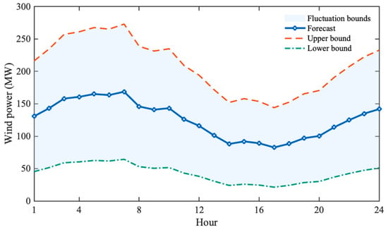
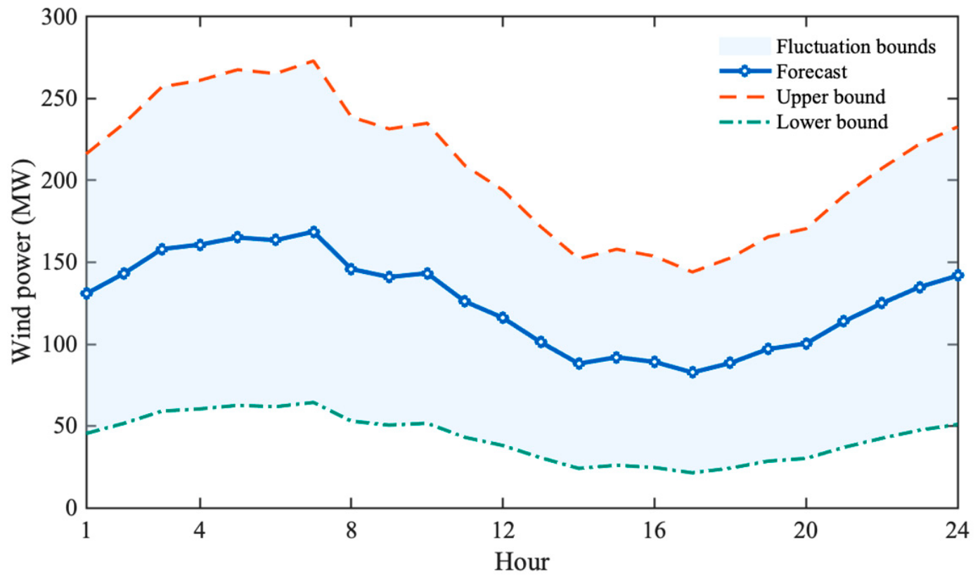
To characterize wind-power uncertainty, a scenario set $\mathsf{\Lambda }$ consisting of 50 wind-power scenarios was generated using Latin hypercube sampling (LHS) [31]. The forecasted hourly wind power and its corresponding upper and lower fluctuation bounds were adopted from the regional power-system case study reported in [30] and were illustrated in Figure 1. These bounds defined the admissible range of wind-power deviations for each scheduling period, within which the sampled wind-power outputs were constrained to remain.

Figure 1. Forecasted wind power together with its upper and lower fluctuation bounds.

Since the wind-power deviation ${\delta }_t$ was defined as the deviation relative to the forecasted wind power $p_t^w$, the fluctuation bounds determined the admissible range of ${\delta }_t$. LHS was employed to generate representative samples of ${\delta }_t$. For each time period $t$, the admissible range of ${\delta }_t$ was evenly divided into 50 subintervals, and one sample was randomly drawn from each subinterval, resulting in 50 candidate values of ${\delta }_t$. One value was then selected from each time period and combined to form a complete wind-power scenario $\delta =\left\{{\delta }_t:t=1,2\dots ,T\right\}$. Repeating this procedure generated a scenario set $\mathsf{\Lambda }$ consisting of 50 wind-power scenarios. The same scenario set was used for the compared UC formulations to ensure a consistent comparison. The resulting 24 h scenarios contained different combinations of hourly wind-power deviations within the prescribed fluctuation bounds. These scenarios allowed the effects of different temporal wind-power variation patterns on unit commitment decisions to be examined over the entire scheduling horizon. However, the LHS-based scenario generation does not explicitly preserve the temporal dependence of wind-power forecast errors, which is a limitation of the current scenario representation.

For the 10-unit system, the initial commitment states were specified as [1, 1, 0, 0, 0, 0, 0, 0, 0, 0], where 1 and 0 denoted committed and decommitted units, respectively. The corresponding initial on/off durations were [8, 8, −5, −5, −6, −3, −3, −1, −1, −1] h, where positive and negative values represented consecutive on- and off-durations before the scheduling horizon, respectively. The initial generation outputs were [150, 150, 0, 0, 0, 0, 0, 0, 0, 0] MW, with the two initially committed units operating at their minimum generation limits. These initial conditions were used as boundary conditions for the minimum on/off-time and ramping constraints. For the 40-unit and 100-unit systems, the initial conditions were constructed by repeating the corresponding 10-unit vectors four and ten times, respectively. The numerical tolerances for power-balance feasibility, generation-limit violations, and ramping-constraint violations were set to 10⁻⁴ MW, 10⁻⁶ MW, and 10⁻⁶ MW, respectively.

In the proposed TBSRUC formulation, the performance threshold $B$ was used to identify bad scenarios. In this work, $B$ was defined based on a reference expected operating cost $\widehat{E}$, where $\widehat{E}$ was estimated using a heuristic optimization procedure that minimized the average operating cost over the wind-power scenarios. The threshold was then defined as $B=\alpha \widehat{E}$, where $\alpha$ was the threshold coefficient. For the model and algorithm comparisons presented in Section 4.2 and Section 4.3, $\alpha$ was set to 1.010. For each experiment, the threshold was kept fixed throughout the optimization process. Consequently, the resulting threshold values were $B$ = 535,516.760, 2,152,784.989, and 5,378,875.598 for the 10-unit, 40-unit, and 100-unit systems, respectively.

The main parameters of MAUN included the population size $\mathit{NP}$, crossover rate $\mathit{CR}$, and mutation rate $\mathit{MR}$. These parameters were determined based on preliminary tests. For the 10-unit and 40-unit systems, the parameter configuration $\mathit{NP}=20$, $\mathit{CR}=0.85$, and $\mathit{MR}=0.05$ was adopted. For the 100-unit system, a larger population size $\mathit{NP}=30$ was used, while the crossover and mutation rates were adjusted to $\mathit{CR}=0.80$ and $\mathit{MR}=0.06$. The prescribed computational time limit was used as the stopping criterion. The time limits were determined through preliminary convergence tests, and the same time limit was applied to all compared algorithms for each system to ensure a fair comparison. Each algorithm was independently executed 20 times, with fixed search-time limits of 90, 190, and 900 s for the 10-, 40-, and 100-unit systems, respectively.

4.2. Comparison of UCP Formulations

To investigate the characteristics of the proposed TBSRUC formulation, comparisons were conducted with two representative unit commitment formulations under wind-power uncertainty, namely stochastic unit commitment (SUC) [32] and worst-case robust unit commitment (WRUC) [19]. Since the present study adopted a finite scenario representation without assigning occurrence probabilities to individual scenarios, SUC was implemented by minimizing the average operating cost over all scenarios, whereas WRUC minimized the worst-scenario operating cost. In contrast, TBSRUC minimized the sum of squared operating-cost degradations relative to the performance threshold under bad scenarios. Consequently, the three formulations represented three different philosophies for handling uncertainty, namely risk-neutral optimization, worst-case protection, and threshold-based robustness enhancement.

For a fair comparison, the three formulations were solved using the same population-based search framework. The same initialization strategy, population evolution procedure, constraint-repair procedure, ED solver, and stopping criterion were employed for all formulations. The difference among the three formulations lay in their optimization objectives, with SUC, WRUC, and TBSRUC minimizing expected operating cost (EC), worst-scenario cost (WSC), and PT, respectively. Nevertheless, the solutions obtained from all three formulations were evaluated using the same performance indicators to enable a comprehensive comparison. To evaluate the economic performance and robustness of the three formulations, the EC and WSC were considered. Table 1 reports the mean values and standard deviations (SDs) of these two indicators over multiple independent runs.

Table 1. Comparison of SUC, WRUC, and TBSRUC across different system scales.

System	Formulation	WSC Mean	WSC SD	EC Mean	EC SD
10-unit	SUC	540,446.98	2987.49	531,489.25	2989.49
	WRUC	538,051.36	2643.66	534,446.68	3272.21
	TBSRUC	539,500.39	3149.44	532,831.72	2187.02
40-unit	SUC	2,174,092.04	3060.53	2,143,597.43	5391.26
	WRUC	2,171,116.39	4986.79	2,147,801.97	3951.90
	TBSRUC	2,173,285.51	9201.29	2,146,457.08	9683.93
100-unit	SUC	5,398,652.86	4761.03	5,326,543.04	13,469.29
	WRUC	5,392,640.27	14,563.16	5,334,513.73	3967.55
	TBSRUC	5,396,546.31	5248.76	5,327,898.30	3069.81

As shown in Table 1, the three formulations exhibited different characteristics because different performance criteria were optimized. The SUC formulation consistently achieved the lowest EC, whereas the WRUC formulation achieved the smallest WSC across all three benchmark systems. In contrast, the proposed TBSRUC exhibited intermediate WSC and EC values between those of SUC and WRUC. These results indicated that the proposed threshold-based formulation maintained competitive economic performance without exclusively minimizing either the expected or worst-scenario operating cost. Compared with these two representative formulations, TBSRUC exhibited distinct threshold-based robustness characteristics while maintaining competitive economic performance under the considered experimental settings.

4.3. Effectiveness of UN Structure

To evaluate the effectiveness of the UN structure, MAUN was compared with a memetic algorithm with a mean-scenario neighborhood (MAMN). In addition, binary particle swarm optimization (BPSO) and a conventional memetic algorithm (MA) were introduced as benchmark algorithms to further evaluate the solution performance of MAUN. MAUN and MAMN employed the same population evolution, constraint-repair, ED, solution-evaluation, and stopping procedures. The difference between the two algorithms lay in the neighborhood structure used for local search. MA employed the same population evolution procedure as MAUN but without the scenario-based local search. BPSO was selected as a representative classical population-based metaheuristic for binary optimization, providing a benchmark with a different search mechanism from MAUN. It updated the binary commitment schedules based on particle velocities and personal and global best solutions. All four algorithms adopted the same initial population, constraint-repair procedure, solution-evaluation method, and computational time limit for each system.

For the current best solution, MAMN constructed a mean-value scenario based on all bad scenarios in its TBS. When the TBS is empty, the local-search stage of MAMN is skipped, following the same fallback rule as MAUN. The wind-power deviation at hour $t$ under the mean-value scenario was calculated as

$$\overline{{\delta }_t}={\displaystyle \frac{1}{BSN}}\sum _{{\delta \in \Lambda }_B\left(\mathit{x}\right)}{\delta }_t , t=1,2,\dots ,T$$

(23)

The critical wind-deficit and wind-surplus periods were identified under the resulting mean-value scenario, and the corresponding single-scenario neighborhood was generated using the same neighborhood operations as those described in Section 3.3. In contrast, MAUN constructed the UN by uniting the single-scenario neighborhoods associated with all individual bad scenarios in the TBS. Therefore, the comparison between MAUN and MAMN was conducted to investigate whether directly exploiting the neighborhood information associated with individual bad scenarios could improve the local search.

The relative deviation percentage ($RDP$) was calculated to evaluate the solution performance of the four algorithms as follows.

$$RDP={\displaystyle \frac{{PT}_{avg}-{PT}_{best}}{{PT}_{best}}}\times 100\%$$

(24)

where ${\mathit{PT}}_{\mathit{avg}}$ denotes the average PT value obtained over multiple runs, and ${PT}_{best}$ denotes the best PT value obtained among the four compared algorithms for the corresponding system. A smaller $RDP$ value indicates better solution quality. When the best PT reference is zero, RDP is undefined, and the corresponding average PT values is reported instead.

Table 2 reports the $RDP$ values of BPSO, MA, MAMN, and MAUN on the 10-unit, 40-unit, and 100-unit systems over multiple independent runs. As shown in Table 2, MAUN obtained the lowest $RDP$ values among the four algorithms across all three system scales, suggesting that MAUN achieved better PT performance in the reported experiments. In particular, the comparison between MAUN and MAMN showed that retaining the neighborhood information associated with individual bad scenarios was more effective in reducing PT than constructing a single neighborhood based on their mean-value scenario. Moreover, the comparisons with BPSO and MA further supported the effectiveness of MAUN relative to the selected benchmark algorithms with different search mechanisms.

Table 2. Performance comparison of BPSO, MA, MAMN, and MAUN across different system scales.

System	Algorithm	$\mathit{R}\mathit{D}\mathit{P}$ (%)
10-unit	BPSO	15,757.40
	MA	16,672.02
	MAMN	26,356.76
	MAUN	2036.15
40-unit	BPSO	59,073.80
	MA	15,798.24
	MAMN	29,546.56
	MAUN	251.61
100-unit	BPSO	6,648,995.08
	MA	347,611.88
	MAMN	624,630.12
	MAUN	1830.56

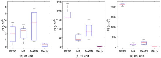
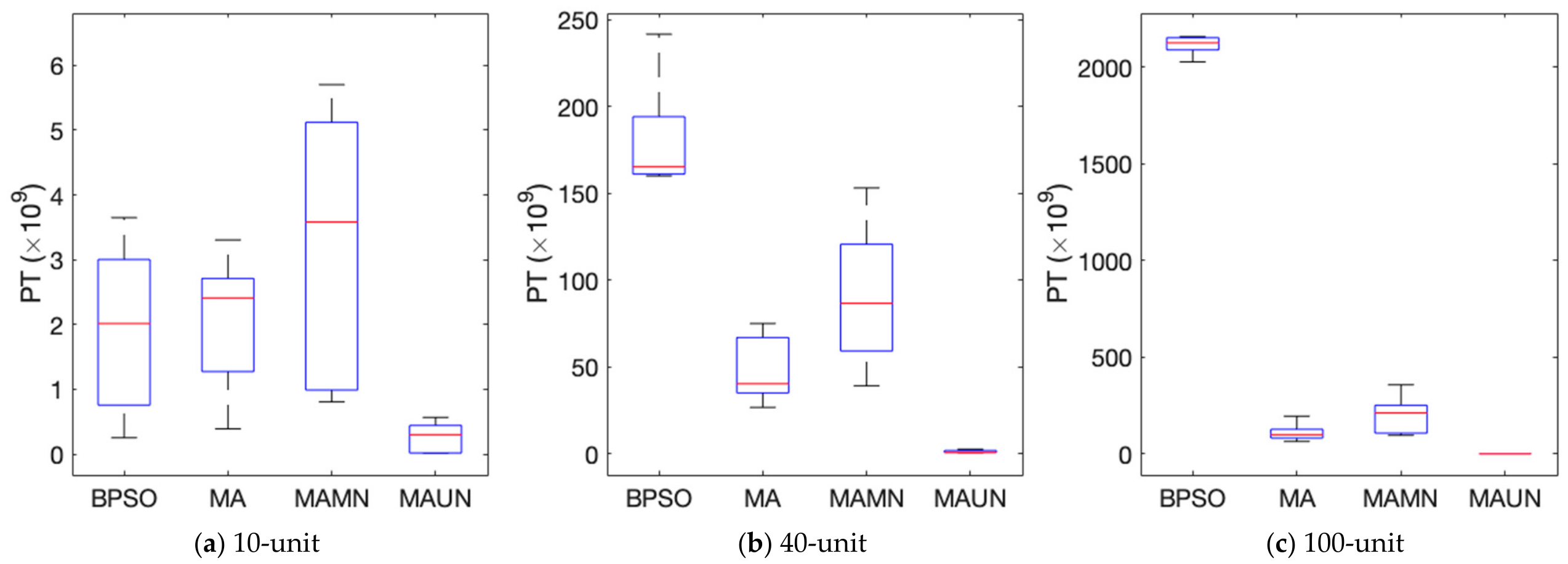
Figure 2 presents the distributions of the final PT values obtained by BPSO, MA, MAMN, and MAUN over multiple independent runs. It can be seen that MAUN generally obtains lower PT values than the other three algorithms across the three system scales. On the 10-unit system, MAUN exhibited the lowest median PT, although its distribution still showed noticeable variability. On the 40-unit and 100-unit systems, the PT values obtained by MAUN were concentrated in substantially lower ranges than those obtained by BPSO, MA, and MAMN, with relatively small dispersion. These results further indicate that MAUN achieved better solution quality than the selected benchmark algorithms, while the comparison with MAMN supports the effectiveness of directly exploiting the neighborhood information associated with individual bad scenarios. However, the statistical significance of the observed performance differences was not evaluated in this study.

Figure 2. Boxplots of final PT distributions obtained by BPSO, MA, MAMN, and MAUN over multiple independent runs.

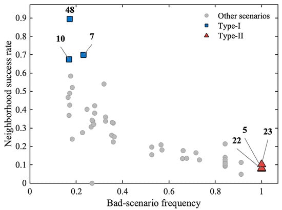
To further examine the contribution of individual bad scenarios to the UN-based local search, scenario-level neighborhood information was collected at each generation over multiple independent runs on the 10-unit system. Figure 3 presents the relationship between the bad-scenario frequency and neighborhood success rate of each scenario. The bad-scenario frequency was defined as the proportion of active local-search iterations in which a scenario belonged to the TBS. The neighborhood success rate was defined as the proportion of its occurrences in the TBS for which the corresponding single-scenario neighborhood generated at least one neighboring solution with a lower PT value than the current best solution after constraint repair and evaluation. To illustrate the differences between scenario occurrence and neighborhood effectiveness, two representative groups of scenarios were identified according to their relative positions in Figure 3. Type-I scenarios were characterized by relatively low bad-scenario frequencies but high neighborhood success rates, whereas Type-II scenarios exhibited high bad-scenario frequencies but low neighborhood success rates. These types were used to distinguish contrasting scenario characteristics.

Figure 3. Relationship between bad-scenario frequency and neighborhood success rate on the 10-unit system.

As shown in Figure 3, substantial differences in neighborhood effectiveness were observed among the bad scenarios. The representative scenarios were selected quantitatively rather than by visual inspection. The median bad-scenario frequency and neighborhood success rate were calculated across scenarios with valid neighborhood-evaluation records. Type-I candidates had frequencies at or below the median and success rates at or above the median; the three with the highest success rates were selected, with ties resolved by lower frequency and then scenario index. Type-II candidates had frequencies at or above the median and success rates at or below the median; the three with the highest frequencies were selected, with ties resolved by lower success rate and then scenario index.

Scenarios 48, 10, and 7 were selected as representative Type-I scenarios, exhibiting relatively low bad-scenario frequencies but high neighborhood success rates. In contrast, scenarios 22, 5, and 23 were selected as representative Type-II scenarios, with high bad-scenario frequencies but substantially lower neighborhood success rates. These results indicate that frequent occurrence in the TBS does not necessarily imply that a scenario provides effective neighborhood information.

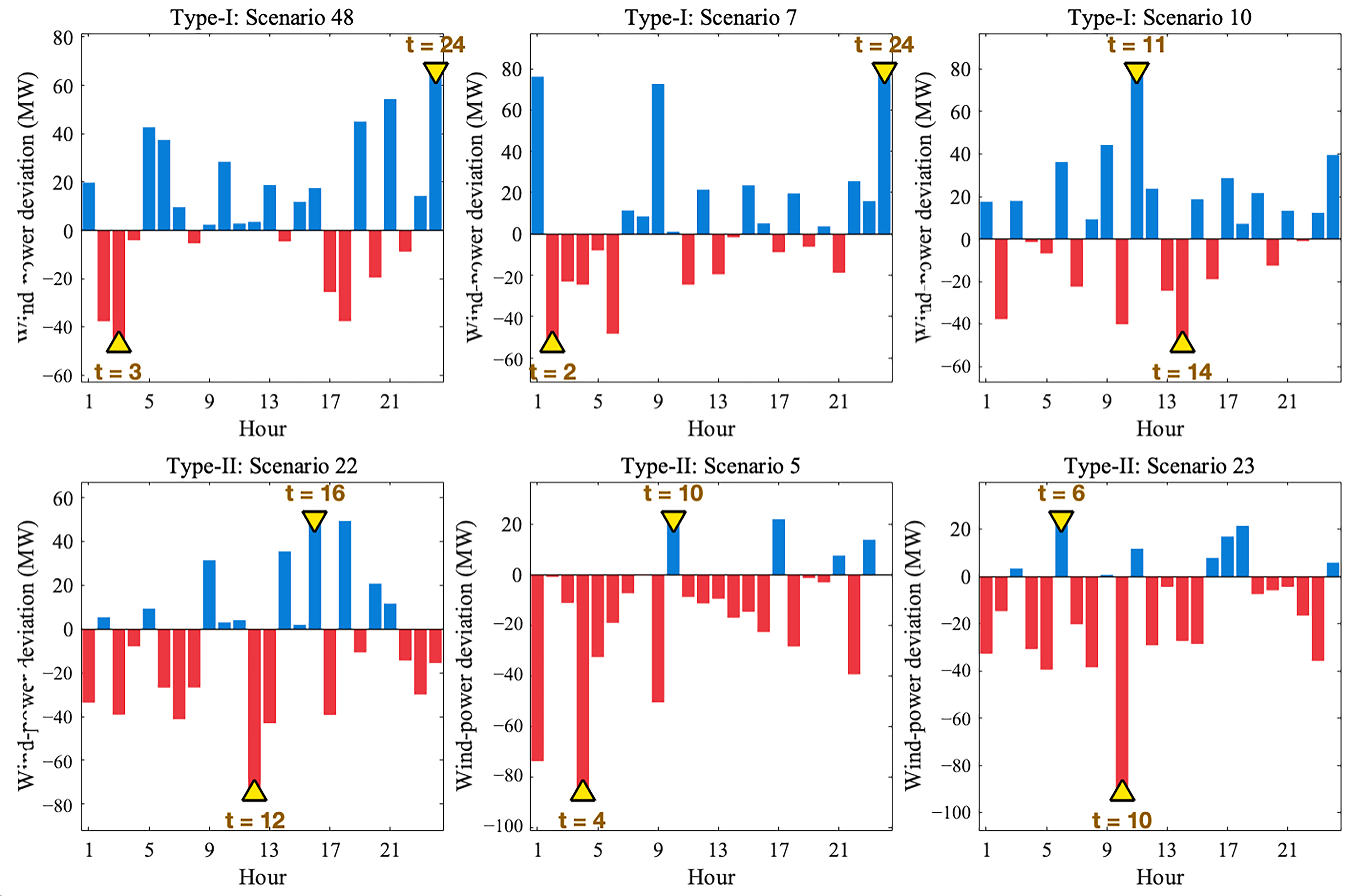
To further illustrate how individual bad scenarios contribute different neighborhood information, Figure 4 presents the wind-power deviation patterns of the representative Type-I and Type-II scenarios. The horizontal axis represents the 24 scheduling hours, while the vertical axis represents the wind-power deviation (MW) relative to the forecast value. The zero line corresponds to the forecast wind-power output, with blue bars indicating positive deviations (wind-power surplus) and red bars indicating negative deviations (wind-power deficit). The yellow downward and upward triangles mark the critical wind-surplus and wind-deficit periods, respectively, and the accompanying labels indicate their corresponding hours (e.g., t = 24 denotes hour 24).

Figure 4. Wind-power deviation patterns and scenario-specific critical periods of representative Type-I and Type-II scenarios on the 10-unit system.

Although the same neighborhood operations were applied to a common commitment schedule, the two critical periods were identified separately for each scenario based on its wind-power deviation pattern. For example, the critical wind-deficit and wind-surplus periods were hours 3 and 24 for scenario 48, respectively, whereas they were hours 12 and 16 for scenario 22. Therefore, even when the same neighborhood operations were applied to the same commitment schedule, different scenarios could generate different neighboring solutions because the operations were performed at different critical periods. By combining the neighborhoods constructed from individual bad scenarios, the UN structure retained multiple scenario-specific search directions that could be lost when the bad scenarios were represented by a single mean-value scenario.

The results in Figure 3 and Figure 4 indicated that individual bad-scenarios provided heterogeneous neighborhood information. While Figure 3 showed that bad-scenario frequency did not necessarily correspond to neighborhood effectiveness, Figure 4 illustrated how scenario-specific critical periods could lead to different neighboring solutions even when the same neighborhood operations were applied. Therefore, preserving the neighborhood information associated with individual bad scenarios allowed the UN structure to explore multiple search directions that might otherwise have been overlooked when these scenarios were represented by a single mean-value scenario.

4.4. Sensitivity Analysis

To examine the sensitivity of the proposed approach to key experimental settings, two analyses were conducted. The first investigated the influence of the performance threshold on the robustness and economic performance of the resulting commitment schedules. The second examined how the number of wind-power scenarios affected solution performance and computational effort.

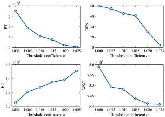
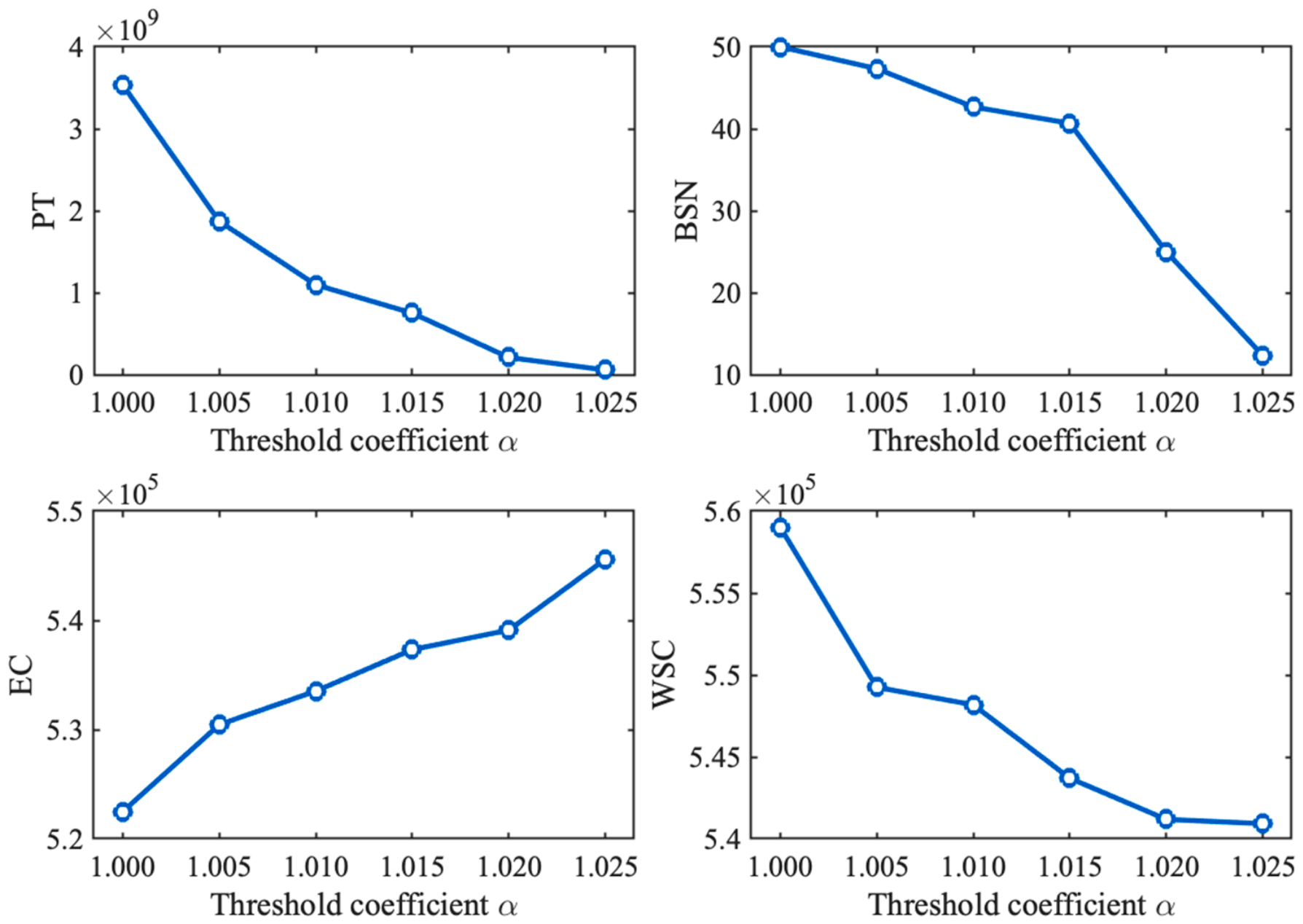
To investigate the influence of the threshold on the performance of TBSRUC, a sensitivity analysis was conducted on the 10-unit system. The threshold was defined as $B=\alpha \widehat{E}$, where $\widehat{E}$ denotes the reference expected cost. Different threshold levels were obtained by setting $\alpha$ to 1.000, 1.005, 1.010, 1.015, 1.020, and 1.025. For each threshold level, the TBSRUC model was independently optimized using MAUN, and the resulting commitment schedules were evaluated in terms of PT, BSN, EC, and WSC. This analysis was conducted to examine how the threshold affected the identification of bad scenarios and the trade-offs among the resulting performance indicators.

As shown in Figure 5, both PT and BSN decreased as the threshold coefficient increased. A higher threshold raised the cost level used to identify bad scenarios and calculate their penalties. Since the commitment schedules were independently optimized at each threshold level, the observed changes in PT and BSN reflected both the threshold settings and the resulting solutions. Meanwhile, EC increased, whereas WSC decreased with increasing $\alpha$, indicating an observed trade-off between economic performance and robustness within the tested threshold range. At lower thresholds, more scenarios were included in the TBS, and the optimization considered the operating costs of a broader range of scenarios, resulting in lower expected costs. At higher thresholds, fewer scenarios were included in the TBS, and the optimization placed greater emphasis on the operating-cost exceedances of the remaining bad scenarios. Under the tested settings, this change was accompanied by lower WSC and higher EC. These results indicated that the threshold coefficient could be adjusted to produce commitment schedules with different balances between economic performance and robustness.

Figure 5. Sensitivity of PT, BSN, EC, and WSC to the threshold coefficient on the 10-unit system.

To investigate the influence of the number of wind-power scenarios, a sensitivity analysis was conducted on the 10-, 40-, and 100-unit systems. Four scenario-set sizes, namely 25, 50, 75, and 100, were considered. For each scenario-set size, the TBSRUC model was optimized using MAUN, while the other experimental settings remained unchanged. For each system scale, the same performance threshold was maintained across all four scenario-set sizes. The resulting solutions were evaluated in terms of PT, EC, and WSC. PT was additionally normalized by the corresponding scenario count to facilitate comparisons across scenario-set sizes. In addition, the number of objective-function evaluations was recorded to examine the computational effort under different scenario-set sizes.

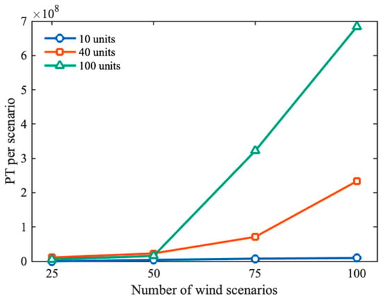
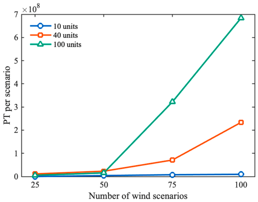
Figure 6 presents the variation in PT per scenario with the number of wind-power scenarios for the 10-, 40-, and 100-unit systems. Since PT is defined as the sum of the squared threshold exceedances over all scenarios, it was divided by the corresponding number of scenarios to reduce the direct influence of scenario-set size on the comparison. The resulting value represents the average penalty per scenario, with zero penalties assigned to scenarios whose operating costs do not exceed the threshold. As shown in Figure 6, PT per scenario remained relatively low in the 10-unit system but increased markedly in the 40- and 100-unit systems, particularly when the number of scenarios exceeded 50. These results indicated that the normalized PT varied with scenario-set size, especially in larger systems. This variation may reflect differences in the scenarios considered and the solutions obtained under the fixed computational budget.

Figure 6. Variation in the PT per scenario with the number of wind-power scenarios across different system scales.

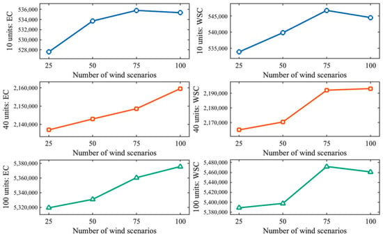
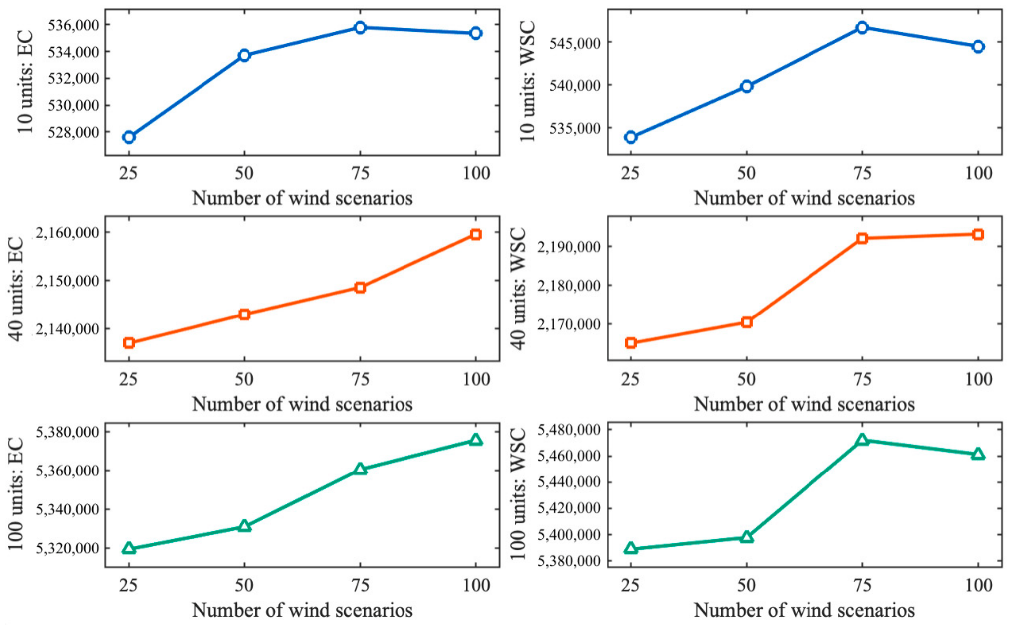
Figure 7 presents the EC and WSC obtained with different numbers of wind-power scenarios for the 10-, 40-, and 100-unit systems. The left column shows EC, while the right column shows WSC, with each row corresponding to a different system scale. In the 10-unit system, both EC and WSC increased from 25 to 75 scenarios and decreased slightly at 100 scenarios. In the 40-unit system, EC and WSC generally increased with the number of scenarios, although the increase in WSC became relatively small between 75 and 100 scenarios. In the 100-unit system, EC increased throughout the tested range, whereas WSC reached its highest value at 75 scenarios before decreasing slightly. Overall, the results show that the number of wind-power scenarios affected the operating costs of the resulting commitment schedules, with different patterns observed across the three system scales.

Figure 7. Variation in EC and WSC with the number of wind-power scenarios across different system scales.

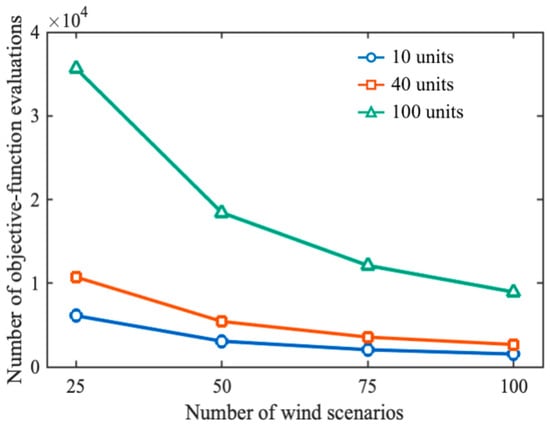
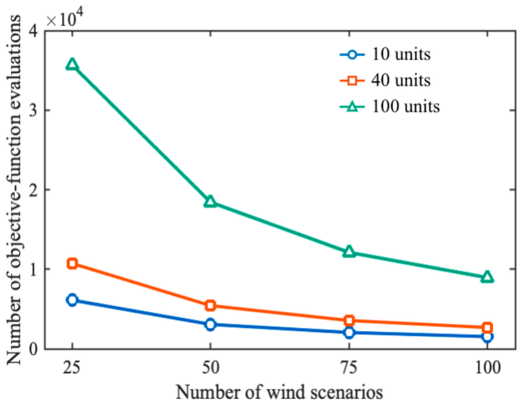
Figure 8 presents the number of objective-function evaluations completed during the MAUN search process under different wind-power scenario counts for the 10-, 40-, and 100-unit systems. One objective-function was defined as the complete search-stage PT evaluation of one candidate commitment schedule across all wind-power scenarios, rather than the evaluation of a single scenario. Each complete PT calculation was counted as one evaluation, regardless of the number of scenarios involved. As shown in Figure 8, the number of objective-function evaluations decreased as the scenario count increased across all three system scales. This is because evaluating a candidate commitment schedule required more scenario-specific economic dispatch calculations when more wind-power scenarios were considered. Consequently, fewer complete candidate solutions could be evaluated within the fixed computational time budget. This trend was particularly pronounced between 25 and 50 scenarios.

Figure 8. Number of objective-function evaluations during the search process under different wind-power scenario counts.

The results in Figure 6, Figure 7 and Figure 8 showed that the number of wind-power scenarios influenced both solution performance and computational effort. Increasing the scenario count generally was associated with higher PT per scenario in the larger systems and affected EC and WSC across all three system scales. Meanwhile, fewer objective-function evaluations were completed as the scenario count increased under the adopted computational limits. These findings highlighted the trade-off between the number of scenarios considered and the computational effort required under a fixed time budget.

5. Conclusions and Future Work

This paper investigated the robust UCP under wind-power uncertainty and formulated a TBSRUC problem. A performance threshold was used to identify the TBS, and the sum of squared operating-cost degradations relative to the threshold under bad scenarios was minimized. In this way, the proposed formulation considers both the number of bad scenarios and the degree of performance degradation under bad scenarios.

To solve the formulated TBSRUC problem, a MAUN was developed. For the current best solution, a single-scenario neighborhood was constructed for each bad scenario in its TBS according to the critical wind-deficit and wind-surplus periods, and these neighborhoods were united to form the UN. A unified multi-scenario constraint-repair mechanism was also employed to maintain the feasibility of commitment schedules under multiple wind-power scenarios.

Computational tests were conducted on benchmark systems with different scales. The comparison with SUC and WRUC showed that the three formulations exhibited different solution characteristics according to their respective optimization criteria, with SUC achieving the lowest EC, WRUC achieving the lowest WSC, and TBSRUC exhibiting intermediate values under the tested settings. The comparisons between MAUN and the benchmark algorithms showed that MAUN achieved lower PT values across the three system scales, while the comparison with MAMN supported the effectiveness of the UN structure. The scenario-level analysis further revealed that individual bad scenarios provided heterogeneous neighborhood information. Scenarios that frequently belonged to the TBS did not necessarily generate more effective neighborhoods, and representative scenarios with different neighborhood effectiveness exhibited distinct temporal wind-power deviation characteristics. The threshold sensitivity analysis showed that different threshold coefficients produced different trade-offs between EC and WSC. The scenario-count sensitivity analysis further showed that solution performance varied with the number of wind-power scenarios, while the number of completed objective-function evaluations decreased as more scenarios were considered under the fixed computational time budget. These results supported the effectiveness of exploiting scenario-specific neighborhood information and highlighted the importance of threshold selection and computational budget considerations.

Future research will investigate the proposed TBSRUC framework for larger-scale power systems and more complex uncertainty environments. In particular, scenario generation based on historical wind-power forecast errors, with consideration of temporal dependence and other relevant statistical characteristics, together with out-of-sample validation, will help further evaluate the applicability and generalizability of the proposed approach. Further improvements in computational efficiency may also be considered for solving large-scale TBSRUC problems. In addition, future work will explore less conservative commitment-repair strategies and alternative neighborhood-generation methods, including the consideration of multiple critical periods, to address the limitations of the current repair and neighborhood-selection procedures.

References

- Padhy, N.P. Unit Commitment-a Bibliographical Survey. IEEE Trans. Power Syst. 2004, 19, 1196–1205. [Google Scholar] [CrossRef] [Scilit]
- Morales-España, G.; Latorre, J.M.; Ramos, A. Tight and Compact MILP Formulation for the Thermal Unit Commitment Problem. IEEE Trans. Power Syst. 2013, 28, 4897–4908. [Google Scholar] [CrossRef] [Scilit]
- Datta, D. Unit Commitment Problem with Ramp Rate Constraint Using a Binary-Real-Coded Genetic Algorithm. Appl. Soft Comput. 2013, 13, 3873–3883. [Google Scholar] [CrossRef] [Scilit]
- Papavasiliou, A.; Oren, S.S. Large-Scale Integration of Deferrable Demand and Renewable Energy Sources. IEEE Trans. Power Syst. 2014, 29, 489–499. [Google Scholar] [CrossRef] [Scilit]
- Quan, H.; Srinivasan, D.; Khambadkone, A.M.; Khosravi, A. A Computational Framework for Uncertainty Integration in Stochastic Unit Commitment with Intermittent Renewable Energy Sources. Appl. Energy 2015, 152, 71–82. [Google Scholar] [CrossRef] [Scilit]
- Xiong, P.; Jirutitijaroen, P.; Singh, C. A Distributionally Robust Optimization Model for Unit Commitment Considering Uncertain Wind Power Generation. IEEE Trans. Power Syst. 2017, 32, 39–49. [Google Scholar] [CrossRef] [Scilit]
- Jiang, B.; Guo, C.; Chen, Z. Frequency Constrained Unit Commitment Considering Reserve Provision of Wind Power. Appl. Energy 2024, 361, 122898. [Google Scholar] [CrossRef] [Scilit]
- Ilyushin, P.V.; Georgievsky, I.D. Review of Methods for Improving the Maneuverability of Power Plants with an Increase in the Share of Wind and Solar Power Plants in Regional Power Systems. Power Technol. Eng. 2024, 58, 463–470. [Google Scholar] [CrossRef] [Scilit]
- Sigitov, O.Y. Characteristics of Wind and Solar Power Plants Operation in the Energy System. Power Technol. Eng. 2025, 58, 824–830. [Google Scholar] [CrossRef] [Scilit]
- Zhang, N.; Hu, Z.; Han, X.; Zhang, J.; Zhou, Y. A Fuzzy Chance-Constrained Program for Unit Commitment Problem Considering Demand Response, Electric Vehicle and Wind Power. Int. J. Electr. Power Energy Syst. 2015, 65, 201–209. [Google Scholar] [CrossRef] [Scilit]
- Bertsimas, D.; Litvinov, E.; Sun, X.A.; Zhao, J.; Zheng, T. Adaptive Robust Optimization for the Security Constrained Unit Commitment Problem. IEEE Trans. Power Syst. 2013, 28, 52–63. [Google Scholar] [CrossRef] [Scilit]
- Álvarez-Miranda, E.; Campos-Valdés, C.; Rahmann, C. Two-Stage Robust UC Including a Novel Scenario-Based Uncertainty Model for Wind Power Applications. Energy Convers. Manag. 2015, 101, 94–105. [Google Scholar] [CrossRef] [Scilit]
- Morales-España, G.; Lorca, Á.; de Weerdt, M.M. Robust Unit Commitment with Dispatchable Wind Power. Electr. Power Syst. Res. 2018, 155, 58–66. [Google Scholar] [CrossRef] [Scilit]
- Lin, Z.; Chen, H.; Wu, Q.; Huang, J.; Li, M.; Ji, T. A Data-Adaptive Robust Unit Commitment Model Considering High Penetration of Wind Power Generation and Its Enhanced Uncertainty Set. Int. J. Electr. Power Energy Syst. 2021, 129, 106797. [Google Scholar] [CrossRef] [Scilit]
- Li, J.; Zhou, S.; Xu, Y.; Zhu, M.; Ye, L. A Multi-Band Uncertainty Set Robust Method for Unit Commitment with Wind Power Generation. Int. J. Electr. Power Energy Syst. 2021, 131, 107125. [Google Scholar] [CrossRef] [Scilit]
- Zheng, X.; Qu, K.; Lv, J.; Li, Z.; Zeng, B. Addressing the Conditional and Correlated Wind Power Forecast Errors in Unit Commitment by Distributionally Robust Optimization. IEEE Trans. Sustain. Energy 2021, 12, 944–954. [Google Scholar] [CrossRef] [Scilit]
- Zhang, N.; Kang, C.; Xia, Q.; Ding, Y.; Huang, Y.; Sun, R.; Huang, J.; Bai, J. A Convex Model of Risk-Based Unit Commitment for Day-Ahead Market Clearing Considering Wind Power Uncertainty. IEEE Trans. Power Syst. 2015, 30, 1582–1592. [Google Scholar] [CrossRef] [Scilit]
- Pinto, M.S.S.; Miranda, V.; Saavedra, O.R. Risk and Unit Commitment Decisions in Scenarios of Wind Power Uncertainty. Renew. Energy 2016, 97, 550–558. [Google Scholar] [CrossRef] [Scilit]
- Jiang, R.; Wang, J.; Guan, Y. Robust Unit Commitment with Wind Power and Pumped Storage Hydro. IEEE Trans. Power Syst. 2012, 27, 800–810. [Google Scholar] [CrossRef] [Scilit]
- Yuan, S.; Dai, C.; Guo, A.; Chen, W. A Novel Multi-Objective Robust Optimization Model for Unit Commitment Considering Peak Load Regulation Ability and Temporal Correlation of Wind Powers. Electr. Power Syst. Res. 2019, 169, 115–123. [Google Scholar] [CrossRef] [Scilit]
- Wang, B.; Xia, X.; Meng, H.; Li, T. Bad-Scenario-Set Robust Optimization Framework with Two Objectives for Uncertain Scheduling Systems. IEEE/CAA J. Autom. Sin. 2017, 4, 143–153. [Google Scholar] [CrossRef] [Scilit]
- Wang, B.; Wang, X.; Xie, H. Bad-Scenario-Set Robust Scheduling for a Job Shop to Hedge against Processing Time Uncertainty. Int. J. Prod. Res. 2019, 57, 3168–3185. [Google Scholar] [CrossRef] [Scilit]
- Wang, B.; Wang, X.; Lan, F.; Pan, Q. A Hybrid Local-Search Algorithm for Robust Job-Shop Scheduling under Scenarios. Appl. Soft Comput. 2018, 62, 259–271. [Google Scholar] [CrossRef] [Scilit]
- He, Y.; Wang, B. Bad-Scenario-Set Robust Power Economic Dispatch with Wind Power. In Proceedings of the 2019 International Conference on Industrial Engineering and Systems Management (IESM), Shanghai, China, 25–27 September 2019; IEEE: Shanghai, China, 2019; pp. 1–6. [Google Scholar] [CrossRef] [Scilit]
- Wang, B.; Zhang, P.; He, Y.; Wang, X.; Zhang, X. Scenario-Oriented Hybrid Particle Swarm Optimization Algorithm for Robust Economic Dispatch of Power System with Wind Power. J. Syst. Eng. Electron. 2022, 33, 1143–1150. [Google Scholar] [CrossRef] [Scilit]
- Wang, X.; Wang, B.; Hu, H.; Qi, B.; Pan, Q. Threshold-Bad-Scenario-Set Robust Energy Trading Decisions for Interconnected Microgrids Under Uncertain Electricity Price. Chin. J. Electron. 2025, 34, 929–936. [Google Scholar] [CrossRef] [Scilit]
- Dimitroulas, D.K.; Georgilakis, P.S. A New Memetic Algorithm Approach for the Price Based Unit Commitment Problem. Appl. Energy 2011, 88, 4687–4699. [Google Scholar] [CrossRef] [Scilit]
- Dhaliwal, J.S.; Dhillon, J.S. Memetic Binary Differential Evolution to Solve Wind–Thermal Profit Based Unit Commitment Problem. Appl. Soft Comput. 2022, 125, 109105. [Google Scholar] [CrossRef] [Scilit]
- Dhaliwal, J.S.; Dhillon, J.S. Profit Based Unit Commitment Using Memetic Binary Differential Evolution Algorithm. Appl. Soft Comput. 2019, 81, 105502. [Google Scholar] [CrossRef] [Scilit]
- Yuan, T.; Chao, Q.; Toerxun, Y.; Li, Y. Optimized economic and environment-friendly dispatching modeling for large-scale wind power integration. Proc. CSEE 2010, 30, 7–13. (In Chinese) [Google Scholar]
- Xu, Q.; Yang, Y.; Liu, Y.; Wang, X. An Improved Latin Hypercube Sampling Method to Enhance Numerical Stability Considering the Correlation of Input Variables. IEEE Access 2017, 5, 15197–15205. [Google Scholar] [CrossRef] [Scilit]
- Papavasiliou, A.; Oren, S.S.; O’Neill, R.P. Reserve Requirements for Wind Power Integration: A Scenario-Based Stochastic Programming Framework. IEEE Trans. Power Syst. 2011, 26, 2197–2206. [Google Scholar] [CrossRef] [Scilit]
Disclaimer/Publisher’s Note: The statements, opinions and data contained in all publications are solely those of the individual author(s) and contributor(s) and not of MDPI and/or the editor(s). MDPI and/or the editor(s) disclaim responsibility for any injury to people or property resulting from any ideas, methods, instructions or products referred to in the content. |
© 2026 by the authors. Licensee MDPI, Basel, Switzerland. This article is an open access article distributed under the terms and conditions of the Creative Commons Attribution (CC BY) license.