


Abstract
This study analyzed the classification of wastewater failures based on their risk levels in Kayseri’s central districts, utilizing citizen reports submitted to the Kayseri Water and Sewerage Administration. In this classification, Class 0 indicates low-priority failures requiring routine maintenance, whereas Class 1 represents high-priority failures necessitating emergency intervention. To evaluate failure risks, machine learning and deep learning methods, including XGBoost, LightGBM, Wide & Deep, TabTransformer, and SVM, were systematically applied. Among traditional machine learning techniques, XGBoost demonstrated competitive performance among the traditional machine learning models (Accuracy: 0.8833, F1-Score: 0.8806, AUC-ROC: 0.9269). Meanwhile, Wide & Deep achieved the highest Accuracy (0.8917) and F1-Score (0.8894), whereas DCN-v2 achieved the highest AUC-ROC (0.9251). Additionally, Mutual Information and 2D Kernel Density Estimation (2D KDE) analyses revealed localized spatial concentrations in the geographic data. Although these spatial features appear weakly related in standard correlation tests, they provide meaningful spatial information for failure risk classification. Among explainable AI approaches, SHAP analysis has been integrated into the models, and the stability of model performance was assessed using cross-validation metrics. The resulting classification framework may support workforce planning, maintenance prioritization, and operational decision-making in wastewater systems.
1. Introduction
Modern societies rely on complex and intertwined critical infrastructure systems [1]. Sewer infrastructure systems are among the most important infrastructure services provided by local governments. The continuity and functionality of these systems are of great importance for public health and urban quality of life. Nowadays, in wastewater systems, issues such as subsidence within the pipes, blockages in pipes and manholes, reverse slope, clogging, incorrect building connections, internal grease buildup, cracks, etc., occur over time. These malfunctions occur due to various physical, operational, and environmental factors [2]. Additionally, in combined sewer systems (systems that carry both storm water and wastewater), the accumulation of solid matter can lead to blockages and various malfunctions due to the reduction in hydraulic capacity and the re-transportation of solids under high flow conditions, which disrupts system performance [3,4,5,6]. These malfunctions in the sewer lines can lead to environmental pollution and public health issues. Water supply networks and sewage systems are essential infrastructure elements critical to ensuring human well-being. These systems are indispensable for protecting public health and preventing epidemics. However, the aging of infrastructure systems is making strategic planning for maintenance and rehabilitation increasingly important [7]. To achieve this goal, models developed to predict the current condition of sewer systems can serve as an important decision-support tool for planning maintenance, rehabilitation, and investment decisions for the network more effectively and accurately [8]. In recent years, new modeling methods have been proposed and applied in engineering fields, based on rapidly developing machine learning methods and Geographic Information Systems (GIS) technology.
There is no direct study in the literature on predicting the resolution times of malfunction requests received by local governments from citizens. Existing similar studies are few in number and limited in scope. In the study conducted by [9], a series of choices regarding priority criteria for wastewater systems in the Municipality of Bihac, Bosnia and Herzegovina, was intended to be presented. For this study, the VIKOR method, a multi-criteria decision-making method, was applied. With this method, the weight coefficients of the criteria for estimating the resolution time of faults were ranked from highest to lowest, and the weight vectors of the criteria were obtained. In his study, ref. [10] stated that in tasks such as repair and maintenance, information about how long the work will take can only be accessed through assumptions or past experience. He stated that the most important factors in workforce planning are the duration of the work process, transportation, and team availability. Ref. [11] utilized machine learning algorithms in their study to predict response times for user requests. In the study, methods such as Support Vector Machines (SVMs), Naive Bayes, Logistic Regression, and Artificial Neural Networks were used, resulting in high accuracy. The aforementioned study aimed to improve the quality of service in the field of information technology. Ref. [12] conducted a possible forest fire prediction using machine learning methods. Among the factors affecting forest fires, weather conditions, time, topographic structure, and human factors were highlighted; important features were identified based on these factors, and the analysis was completed using classification methods. In their study conducted in 2023, ref. [13] compared various supervised learning algorithms [k-Nearest Neighbors (k-NN), Subspace k-NN, Support Vector Machines (SVM), Random Forest, Bagged Decision Tree, Naive Bayes, and Linear Discriminant Analysis (LDA)] with the unsupervised learning method called Stacked Auto encoders to evaluate the environmental impacts of forest fires in a deep learning-based study. In the study, the simulation results for forest fires were analyzed both qualitatively and quantitatively, and it was concluded that the methods achieved a high level of accuracy. Ref. [14] used hyper parameter-optimized machine learning techniques to predict city-level changes in carbon footprints in Türkiye with high accuracy and analyzed their spatial distributions. In the study, the Bayesian method and hyper-optimized machine learning techniques were used. Nowadays, machine learning-based forecasting approaches are gaining increasing importance in both the public and private sectors for modeling complex processes and developing decision support mechanisms. Especially in local governments, the use of data-driven methods has become inevitable to respond quickly and effectively to increasing service demands. In this context, the ability to predict failures in infrastructure systems in advance plays a critical role in workforce planning and optimizing operational processes. In this study, the aim is to predict the criticality levels of wastewater malfunctions using data from the central districts of Kayseri province. In this context, the research problem was designed in a binary risk classification structure allowing emergency planning for administrations rather than a failure resolution time prediction. Within this scope, various machine learning and deep learning algorithms, including Wide & Deep, DCN-v2, XGBoost, Gradient Boosting, TabTransformer, LightGBM, Deep MLP, Logistic Regression, Extra Trees, Voting Ensemble, AutoInt, ResNet-Tabular, Ridge Classifier, AdaBoost, NODE, and SVM (RBF), have been evaluated together with a GIS-based data structure and hyperparameter optimization. The main objective of the study is to predict failure priorities in advance, thereby accelerating intervention processes, improving workforce utilization efficiency, and enhancing the quality of local government services. To prevent the risk of data leakage, system identities assigned after the failure notification were excluded, and evaluations were conducted solely over physical and geographical parameters known prior to the failure. This study offers a unique contribution by focusing on the failure risk classification problem, which has been addressed only to a limited extent in the literature, integrating GIS-based spatial data with machine learning methods, and supporting the model results with an explainable artificial intelligence approach. Additionally, the comparative evaluation of different algorithms after hyperparameter optimization provides a practical and reliable analysis framework for decision-makers.
2. Materials and Methods
2.1. Study Area and Data
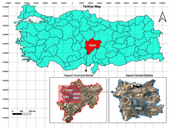
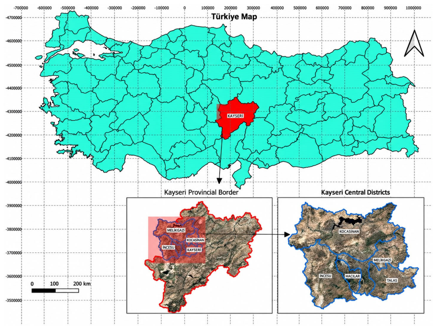
Kayseri is located in the southeastern part of the Central Anatolia Region of Türkiye, in the Middle Kızılırmak section, at the intersection of the Taurus Mountains and the Central Anatolia plateau. The province is located between approximately 37°45′−38°18′ north latitudes and 34°56′−36°58′ east longitudes, with an average elevation of 1071 m. Kayseri, with a population of approximately 1.4 million, has an area of 16,975 km2 [15,16,17]. Its eastern and northeastern borders are adjacent to Sivas, its northern border to Yozgat, its western border to Nevşehir, its southwestern border to Niğde, and its southern borders to the provinces of Adana and Kahramanmaraş (Figure 1).
Figure 1.
The geographical location of the study area.
Including the central districts, it has a total of 16 districts. These are the districts: Kocasinan and Melikgazi in the city center, Akkışla, Bünyan, Felahiye, Develi, Hacılar, İncesu, Pınarbaşı, Özvatan, Talas, Sarıoğlan, Tomarza, Sarız, Yahyalı, and Yeşilhisar. The most important and highest mountain in Kayseri is Mount Erciyes, which stands at 3916 m. Mount Erciyes is a dormant cluster of volcanoes with many subsidiary volcanic peaks on its flanks and slopes. It holds an important place in terms of mountaineering and winter tourism (https://www.kayseri.gov.tr/cografi-yapisi (accessed on 15 September 2026)).
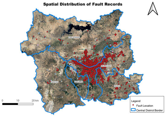
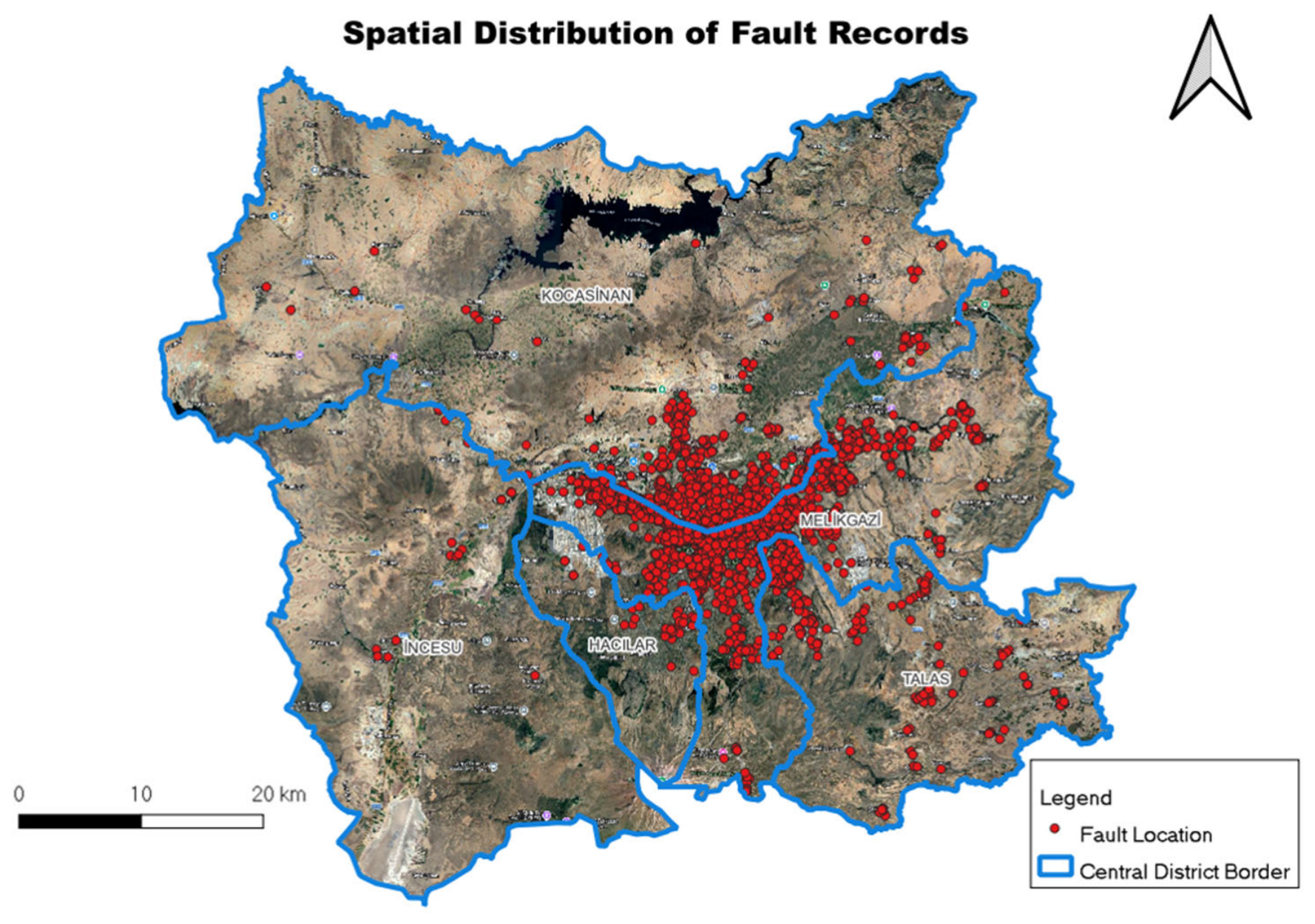
In this study, wastewater failure data collected from the central districts of Kayseri province, namely Kocasinan, Melikgazi, Talas, İncesu, and Hacılar, were used as the study material (Figure 2).
Figure 2.
Spatial distribution of fault records.
Data on a total of 1200 fault records with spatial features, recorded as work orders in the KASKİ database between 2022 and 2025, have been considered. The district-level characteristics of the fault records for the study area are provided in Table 1.
Table 1.
District-level fault data and study area characteristics.
2.2. Methods
Prior to modeling, continuous features were standardized using a standard scaler approach, while the categorical variable pipe_type was transformed using zero-based integer label encoding. For deep learning architectures, the integer-encoded categorical variables were processed through dedicated embedding layers. No class-balancing procedure was applied, and the original target-class distribution was preserved during model development. The modeling process was designed as a binary classification problem in accordance with operational decision-making mechanisms rather than a failure resolution time prediction. In this context, the dependent variable Class 0 indicates low-priority failures that have not lost network functionality and can be scheduled for routine planned maintenance, whereas Class 1 defines high-priority failures requiring emergency intervention. The target labels were obtained directly from the original KASKİ work-order database and were not generated retrospectively by the authors. The operational labels were assigned by KASKİ dispatch operators and field inspection teams at the initial assessment stage of the work-order process according to the severity of network disruption and immediate environmental or public health risks. For modeling purposes, the original operational codes were mapped to Class 0 and Class 1 without changing their underlying meaning. Variables generated after the initial classification or assignment stage were not used to construct or modify the target label and were excluded from the predictive feature set when they posed a risk of target leakage. Work demand codes and team identity numbers derived after the failure notification were not included in the training set on the grounds that they cause data leakage. During the preprocessing stage, continuous features were standardized using a standard scaler approach, while the categorical variable pipe_type was transformed using zero-based integer label encoding. For deep learning architectures, these integer-encoded categorical variables were processed through dedicated embedding layers. Importantly, these category codes were not interpreted as continuous numerical magnitudes in the inferential statistical analyses; pipe_type was excluded from Spearman and ANOVA analyses and was evaluated strictly with categorical association measures such as the Chi-square test and Cramer’s V. In this study, the classification models evaluated include Wide & Deep, DCN-v2, XGBoost, Gradient Boosting, TabTransformer, LightGBM, Deep MLP, Logistic Regression, Extra Trees, Voting Ensemble, AutoInt, ResNet-Tabular, Ridge Classifier, AdaBoost, NODE, and SVM (RBF). Initially, the dataset was divided into 80% training and 20% testing subsets while preserving the spatial block structure. Spatial blocks were defined by applying a K-Means clustering algorithm to the geographic coordinates, partitioning the study area into 5 non-overlapping spatial clusters. One of the five K-Means spatial clusters, representing approximately 20% of the dataset, was reserved exclusively as the independent spatial test holdout. Nested cross-validation was subsequently applied within the spatially separated training data for model selection and hyperparameter optimization. Within the spatially separated training data, a nested cross-validation scheme with 5 outer folds and 3 inner folds was used for model selection and hyperparameter optimization. Consequently, the simultaneous appearance of the same block in the training and test subsets was strictly prevented, ensuring the absolute independence of the final test subset. Although the source work orders cover the 2022–2025 period, the anonymized modeling table utilized in the present analysis did not retain a record-level timestamp or year variable. Therefore, a strictly out-of-time temporal validation could not be performed. This limitation is explicitly acknowledged, and temporal external validation utilizing time-stamped future work orders is recommended for subsequent studies. Hyperparameter optimization was conducted using 50 Optuna trials. Deep learning models were trained using architecture-specific learning rates and batch sizes selected within the search ranges reported in Appendix A Table A1, with dropout rates between 0.1 and 0.3, a fixed random seed (42), and up to 100 epochs with early stopping mechanisms. To reduce statistical uncertainties that may arise from sample size, the obtained results were supported by cross-validation variance metrics, the interaction between categorical variables was examined through Chi-Square independence tests, and the decision processes of the models were made transparent via SHAP analysis.
2.2.1. Wide & Deep
The Wide & Deep method used in the developed wastewater failure prediction application is among the most successful approaches in the literature for learning feature interactions, which are common in tabular data. Initially developed for search engines and recommendation systems, this model combines the ability to “memorize” statistical relationships in structured data with the ability to “generalize” unseen data patterns within a single framework [18]. The architecture operates through the joint optimization of a linear model (Wide) and a feedforward deep neural network (Deep).
2.2.2. DCN-v2
The DCN-v2 method is a modern deep learning architecture designed to automatically and explicitly learn interactions between variables in tabular data. Structurally, it consists of two main parts: a Cross Network, where features are explicitly mixed, and a Deep Network, where non-linear, more abstract patterns are learned [19].
2.2.3. XGBoost
The XGBoost method is a effective ensemble learning algorithm optimized within the framework of gradient boosting, based on decision trees. The biggest difference from standard gradient boosting methods is the use of strict regularization terms added to the objective function and second-order (Hessian) approaches for optimizing the loss function [20].
2.2.4. Gradient Boosting
The Gradient Boosting method is a forward stage-wise machine learning algorithm that combines weak learners (usually decision trees) to create a strong ensemble model. The fundamental philosophy of the algorithm is based on training each new tree to compensate for the errors (residuals) made by the previous model. This process is carried out by optimizing in the direction of the negative gradient of a specified loss function.
2.2.5. TabTransformer
The TabTransformer used in the Water and Sewerage Administration’s pipe failure prediction application is a modern deep learning method that employs self-attention mechanisms to transform categorical features in structured (tabular) datasets into rich contextual representations.
2.2.6. LightGBM
LightGBM (Light Gradient Boosting Machine), positioned in the machine learning module of the Water and Sewerage Administration’s pipe failure prediction system, is an advanced gradient boosting framework that dramatically enhances the training speed and efficiency of decision tree-based algorithms [21].
2.2.7. Deep MLP
The Deep MLP (Deep Multi-Layer Perceptron) method is a feed-forward deep neural network designed to represent non-linear, complex relationships in tabular data in high-dimensional spaces. The architecture consists of sequentially arranged fully connected linear transformation layers with nonlinear activation functions between them.
2.2.8. Logistic Regression
The Logistic Regression used in the Water and Sewerage Administration’s pipe failure prediction model is a fundamental and highly powerful statistical learning algorithm that performs classification by blending linear features within a probabilistic framework.
2.2.9. Extra Trees
The Extra Trees method is an ensemble learning algorithm consisting of decision trees. Despite having significant similarities to the Random Forest architecture, it has two fundamental mathematical differences: First, while each tree is trained, the entire dataset is generally used rather than a bootstrapped subset. Secondly and most importantly, the feature split thresholds at the tree nodes are chosen completely randomly, not through analytical optimization.
2.2.10. Voting Ensemble
The Voting Ensemble method is a meta-learner structure that combines the three tree-based algorithms in the machine learning literature (Random Forest, XGBoost, and LightGBM) into a single prediction mechanism.
2.2.11. AutoInt
The AutoInt (Automatic Feature Interaction Learning) method is a modern neural network designed to automatically learn high-order interactions between features in tabular data. The architecture uses the Multi-Head Self-Attention mechanism, which is widely used in Natural Language Processing to model interactions among features from different fields, including pipe diameter, pipe type, and geographic coordinates [22].
2.2.12. ResNet-Tabular
The ResNet-Tabular method is an adaptation of the Residual Networks architecture, originally developed in image processing, to structured (tabular) data sets [23].
2.2.13. Ridge Classifier
The Ridge Classifier method is a linear model that, unlike traditional classification algorithms, treats the problem as a “Regularized Least Squares” regression.
2.2.14. Adaptive Boosting (AdaBoost)
The AdaBoost (Adaptive Boosting) method is a meta-learning algorithm that aims to obtain a strong classifier by sequentially training weak learners (usually single-depth decision trees or stumps) [24,25].
2.2.15. Neural Oblivious Decision Ensembles (NODE)
In the context of the Water and Sewerage Administration’s pipe failure prediction modeling using deep learning, NODE (Neural Oblivious Decision Ensembles) is a hybrid architecture that transforms the discrete and non-differentiable structure of traditional decision trees into continuous functions [26].
2.2.16. Support Vector Machines (SVM, RBF)
Support Vector Machines (SVMs) used in the Water and Sewerage Administration’s pipe failure prediction modeling are geometric learning algorithms whose primary purpose is to find the hyperplane with the widest margin (the largest decision boundary) that separates data points [27,28,29,30].
2.2.17. Model Configuration and Reproducibility
Model-specific search spaces, final selected hyperparameters, and architecture settings are reported in Appendix A, Table A1. Hyperparameter optimization was conducted using 50 Optuna trials within the validation framework described above. For each machine learning model, Appendix A Table A1 reports the tuned parameters, tested search intervals, and final selected values. For each deep learning architecture, Appendix A Table A1 reports the number of layers, hidden dimensions, dropout rates, optimizer settings, learning-rate settings, batch sizes, epoch limits, early-stopping settings, and random seed. To ensure a fair and consistent comparative evaluation, all deep learning architectures were trained under a unified optimization protocol. Network parameters were updated using the AdamW optimizer. The learning rate and batch size were tuned within the predefined search ranges reported in Appendix A Table A1, and the final settings used for the evaluated deep learning architectures were 1 × 10⁻³ and 128, respectively. A weight decay of 1 × 10⁻⁴ was used, and the learning rate was dynamically adjusted using a CosineAnnealingLR scheduler (T_max = 50, eta_min = 1 × 10⁻⁵). The training process was bounded to a maximum of 100 epochs, and an early-stopping mechanism was implemented to halt training if the validation performance did not improve for 10 consecutive epochs (patience = 10). The random seed used for the final experiments was fixed at 42. Furthermore, the Voting Ensemble model was configured utilizing a soft voting strategy with uniform weights over the individually optimized base estimators. Irrelevant algorithms that were eliminated during the preliminary screening phase have been excluded from the final hyperparameter configurations to preserve methodological focus.
3. Results and Discussion
In the dataset used, a total of 1200 samples were divided, with 960 rows allocated for the training process and 240 rows reserved for testing the models. F1-Score, Specificity, Sensitivity, and AUC-ROC values were accepted as the main performance indicators instead of the accuracy metric, which is sensitive to inter-class distribution inequality. The Results section focuses on analyses supporting target definition, data-leakage assessment, spatial interpretation, model performance, and explainability.
Wide & Deep produced the highest test Accuracy (0.8917) and F1-Score (0.8894) among the evaluated deep learning models, whereas DCN-v2 produced the highest AUC-ROC (0.9251). However, the performance differences among the leading models were small relative to the variability observed across cross-validation folds; therefore, these results are interpreted as broadly comparable rather than as evidence of statistically confirmed superiority of a single model.
3.1. Distribution of the Target Variable in the Training Dataset
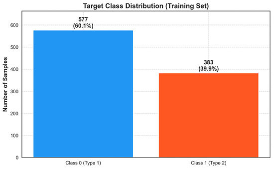
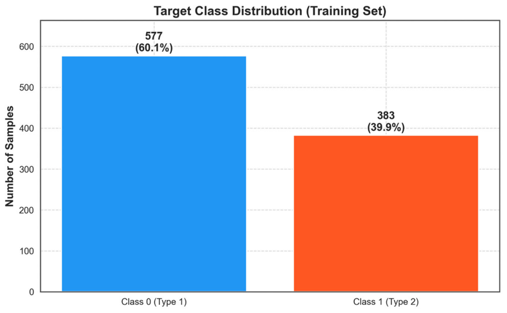
It is observed that the dataset to be used for training machine learning and deep learning models comprises 960 observations (Figure 3). When the proportional distribution of the target variable (fault status) was analyzed, it was determined that records labeled as ‘Class 0’ (low-priority failure) constituted the majority class with 577 records (60.10%), while records labeled as ‘Class 1’ (high-priority failure) represented the minority class with 383 records (39.90%).
Figure 3.
Frequency and proportional distribution of the target variable (low-priority and high-priority failure classes) within the training dataset.
3.2. Monotonic Relationships Between Features and Spearman Rank Correlation Analysis
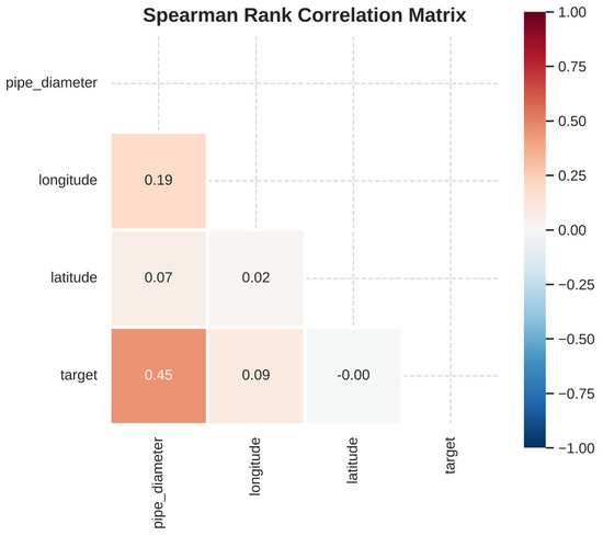
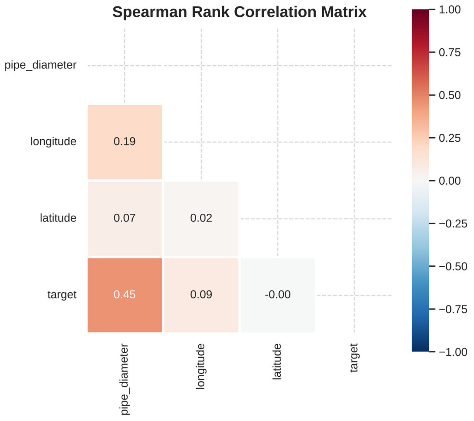
To analyze the statistical interactions between the features and the linear/monotonic effects on the target variable (failure status), the Spearman rank correlation matrix shown in Figure 4 was created. When examining the heat map, the strongest positive relationship with the target variable is with pipe_diameter (r = 0.45). This situation indicates that the main network lines with larger diameters have a statistically higher probability of developing faults. Nominal variables such as work demand identity and pipe type were explicitly excluded from the Spearman correlation analysis to prevent misinterpretation of categorical data as numerical magnitudes. Furthermore, it was determined that operational identifiers would corrupt the external validity of the model, and only physical and geographical parameters were evaluated in continuous correlation tests.
Figure 4.
Spearman rank correlation matrix showing the monotonic relationships between the independent variables (features) in the dataset and the target variable (failure status).
3.3. Geometric Analysis of Fault Profiles in a Binary Attribute Space
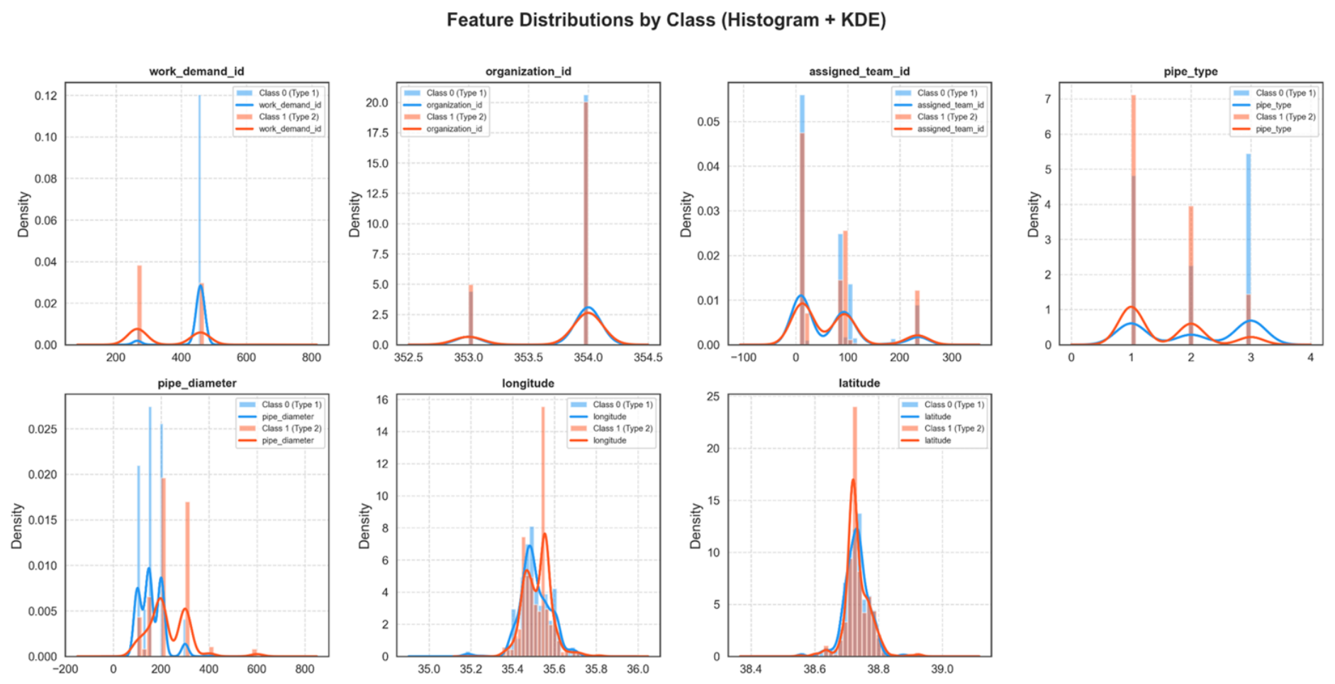
An analysis of the variable distributions by target class (Class 0: low-priority failure, Class 1: high-priority failure) reveals distinct structural differences. Specifically, for the pipe_type variable, it has been determined that Type 3 pipes are predominantly concentrated in the Class 0 (low-priority failure) group, while Type 1 pipes are more frequently observed in the Class 1 (high-priority failure) group. Similarly, for the pipe diameter variable, as the diameter value exceeds 300 mm (especially around 400 mm and 600 mm), the concentration of Class 1 clearly surpasses that of Class 0. This finding supports the previously identified correlation analysis indicating an increased risk of failure in large-diameter pipes.
3.4. Evaluation of Feature Separability
An analysis of the feature distributions revealed that the most distinct class separation was observed in the variables pipe_diameter and pipe_type. While the median diameter of Class 0 hovers around 150 mm with a relatively narrow interquartile range (IQR), the overall data spread (variance) has widened significantly. The distribution of pipe_type also differs notably between the two classes, indicating a distinct relationship with failure status. These statistical shifts (distribution shifts) indicate that these two variables will be highly critical (high-importance) features for the machine learning models.
3.5. Class-Based Feature Characterization with Violin Plots
Unlike box plots, violin plots reveal multimodal patterns in the data, providing deeper insights into the distributional characteristics of failure classes. The most pronounced class separation is observed in the pipe_diameter variable. Class 0, representing low-priority failures, exhibits a sharp density peak in the 150–200 mm range, with density decreasing substantially at larger diameters. In contrast, Class 1, representing high-priority failures, displays a broader distribution, with greater density across the 200–400 mm range and a longer tail extending up to 600 mm. These distributional differences suggest an association between larger pipe diameters and high-priority failures, highlighting pipe diameter as a potentially important feature for failure classification.
3.6. Histogram-KDE-Based Class Separability of Discrete and Continuous Features
Although expressed numerically, the histograms of the categorical identifiers assigned_team_id and work_demand_id show that the data peaks in very narrow ‘spikes’. These local accumulations statistically indicate that the high-priority failures (Class 1, orange bars) have become chronic in the duty areas of certain teams or during specific periods of work demand.
3.7. Probabilistic Failure Trends with Stacked Bar Charts
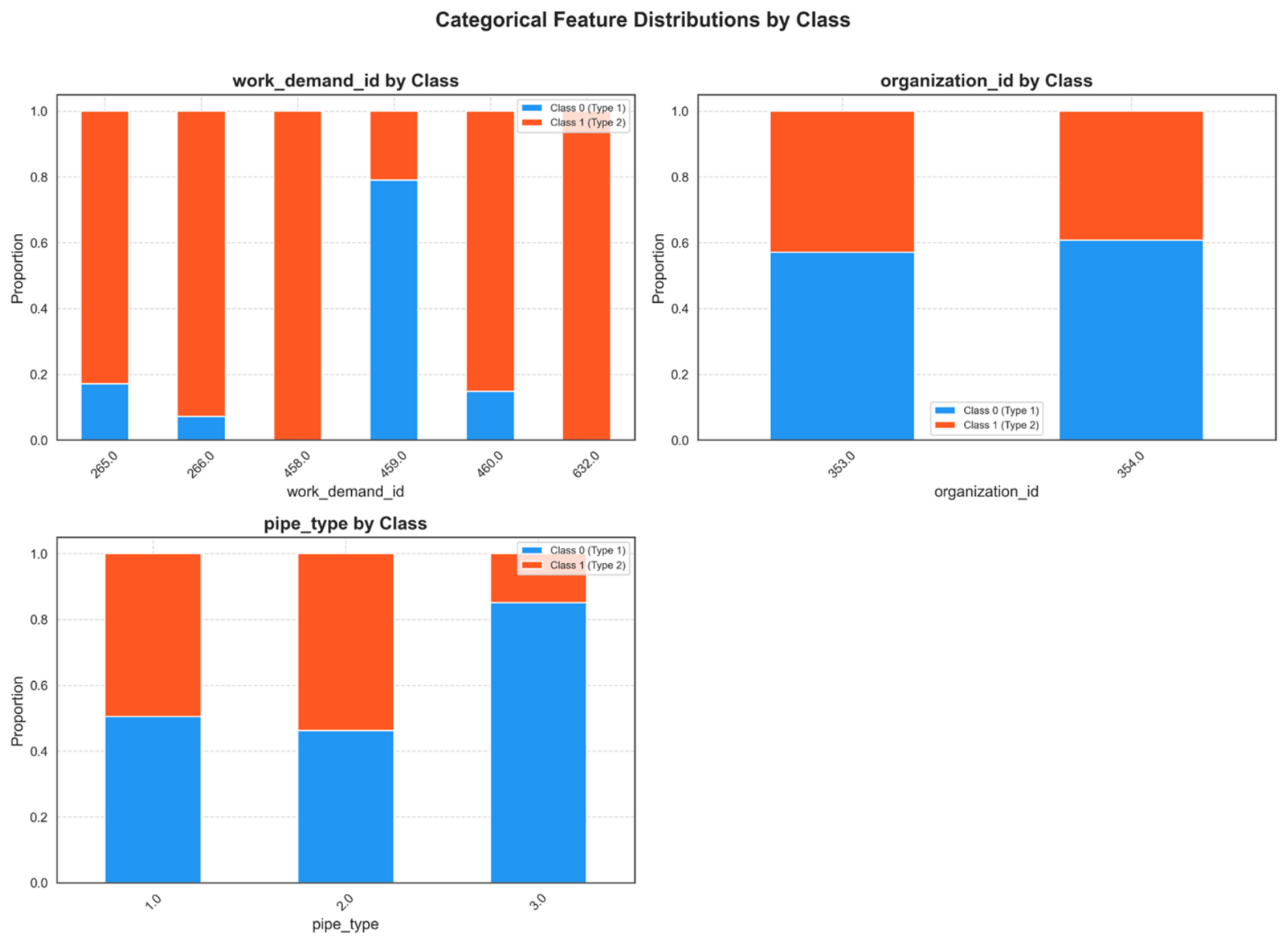
Unlike the previous histograms and density plots, this visual does not display absolute frequencies but rather the normalized probabilistic trends (internal class ratios) within the category (Figure 5). The most striking finding in the graph appears in the work_demand_id variable. It is observed that the job request codes 458.0 and 632.0 consist of 100% orange-colored Class 1 (high-priority failure) category. However, it has been determined that approximately 80% of the 459.0 category belongs to the Class 0 (low-priority failure) profile (Figure 6). Within this scope, since it was determined that the said variables caused target leakage during the prediction process, the relevant features were not included in the model training set to preserve the general structure of the algorithms.
Figure 5.
Distribution matrix showing the absolute frequencies (histogram) and continuous probability density curves (KDE) of the independent variables according to the target classes (class 0: low-priority failure class 1: high-priority failure) simultaneously.
Figure 6.
Normalized proportional distribution of the target variable (class 0/class 1) according to categorical attribute groups.
3.8. Spatial Clustering and Fault Distribution in Geographic Feature Space
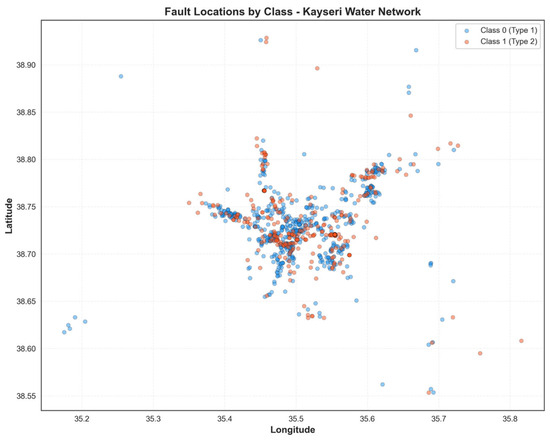
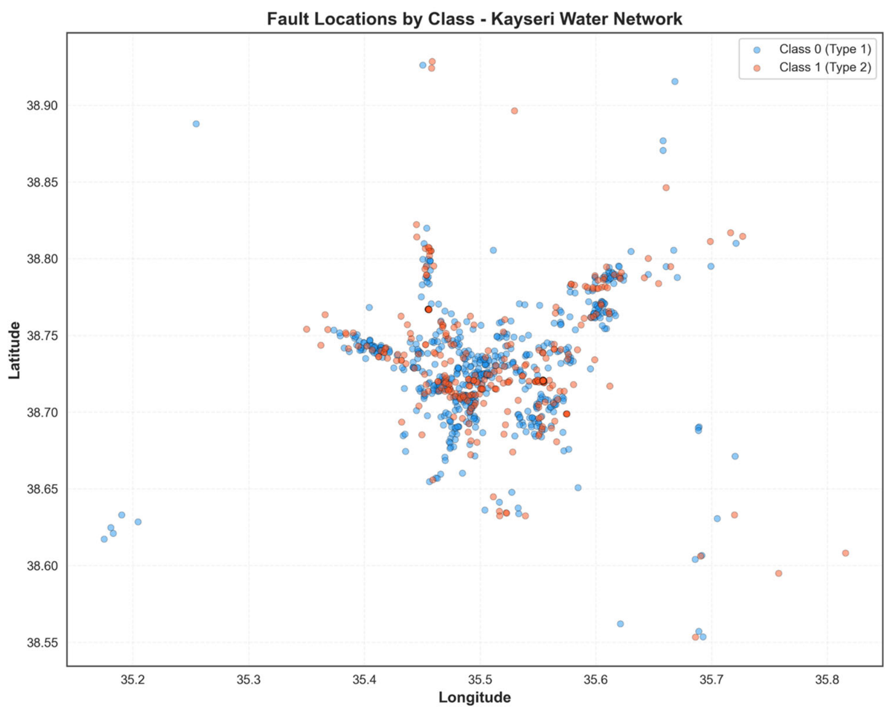
When the graph is examined, it is observed that the distribution of data points on the x (longitude) and y (latitude) axes simulates the physical settlement plan and wastewater network of Kayseri province. The extremely dense clustering in the center represents the city center, while the more sparsely distributed structures around it represent rural or suburban areas. When the coloring based on class labels is analyzed (Class 0: Blue, Class 1: Orange), it is observed that the high-priority failures do not accumulate in a specific geographical direction (for example, only to the north or east of the network); rather, they exhibit a complex spatial pattern that is highly overlapping with the low-priority failure network (Figure 7).
Figure 7.
The distribution and spatial overlap of low-priority (Class 0) and high-priority (Class 1) failure records of the Kayseri wastewater network in the geographic coordinate plane (latitude and longitude).
3.9. Two-Dimensional Density Analysis (2D KDE) and Spatial Density Mapping
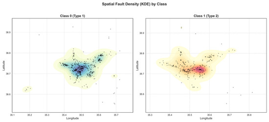
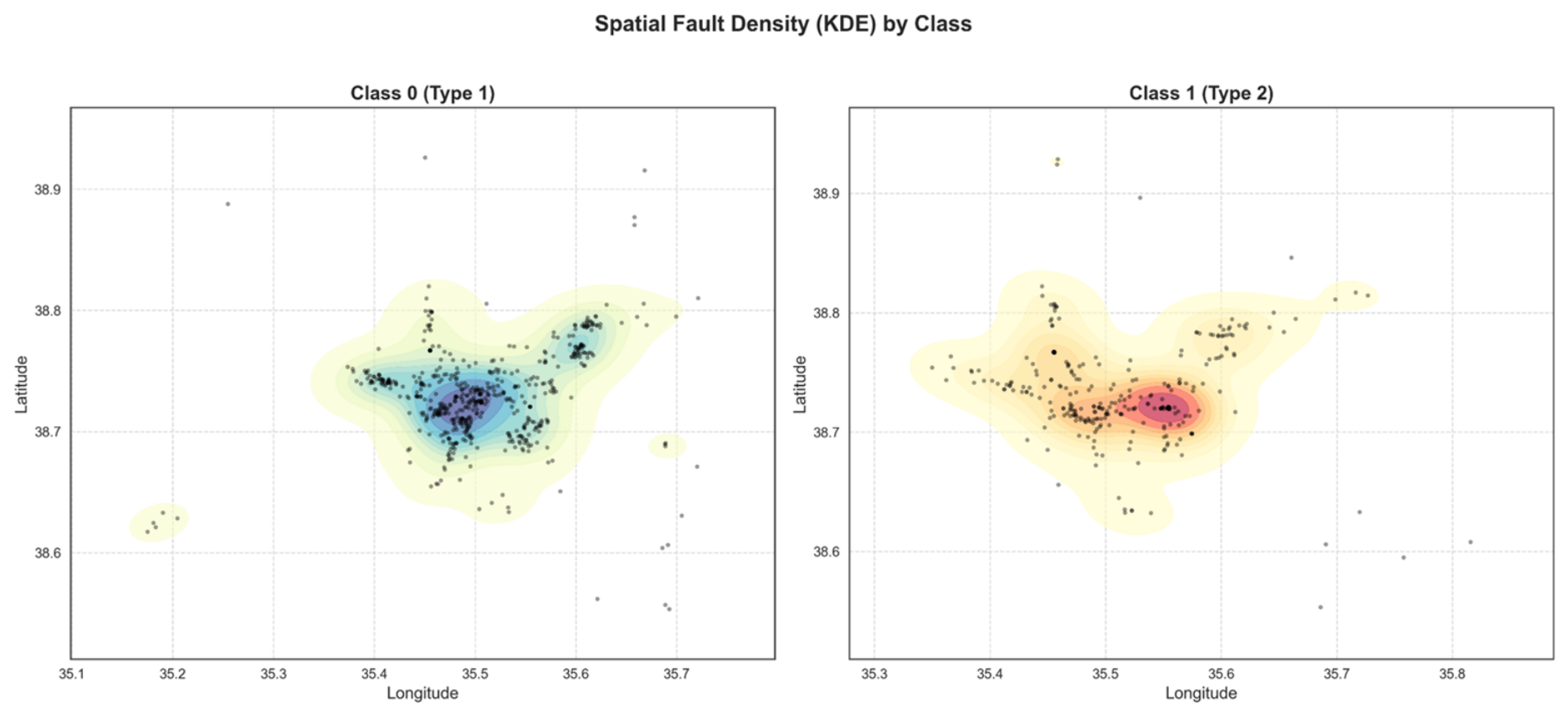
The graph below shows not only where the data is located but also where the probability mass peaks geographically according to the target classes, through topological contours. The blue density center formed by the Class 0 records clusters around a specific core and shows a slight spread toward the northeast; meanwhile, the red/hot density center representing the Class 1 records has experienced a distinct ‘spatial shift’ toward the central-eastern axis of the map. The generated 2D KDE maps were interpreted not directly as a risk map but as spatial accumulations of observed cases depending on the density of network elements (Figure 8).
Figure 8.
Contour maps of the two-dimensional kernel density estimation (2D KDE) of the Class 0 and Class 1 pipe records in the Kayseri water network in the geographic coordinate plane.
3.10. Statistical Dependence Between Categorical Variables and Chi-Squared Analysis
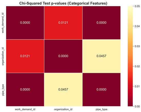
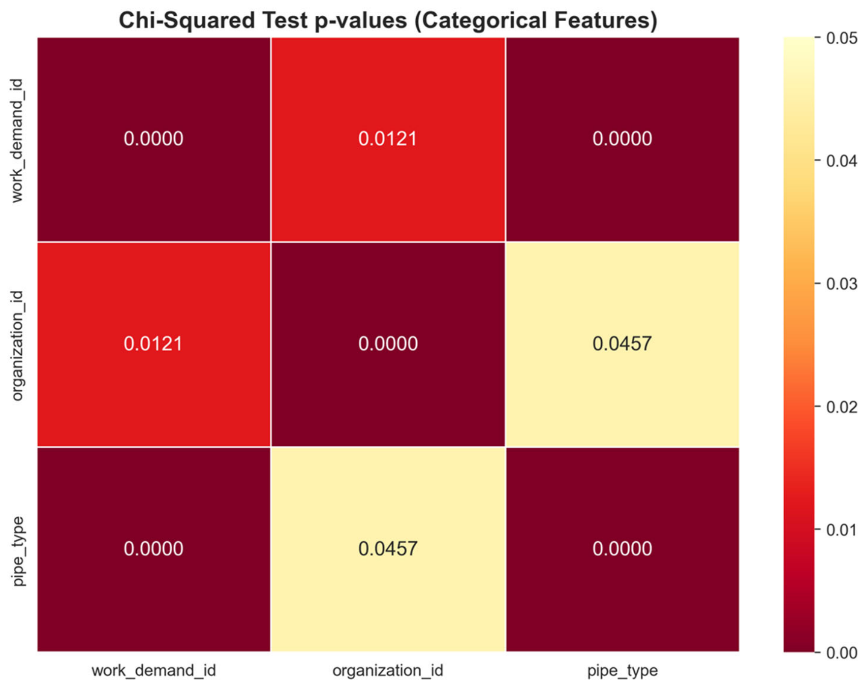
When the heat map was examined, the p-values for all attribute pairs were below the standard statistical significance threshold of $\alpha = 0.05$. Dependence tests of nominal features were performed with Chi-square tests and Cramer V coefficients instead of linear correlation matrices. The most striking finding is that the p-value between work_demand_id (work demand code) and pipe_type (pipe type) is $0.0000$ (dark red). This situation indicates that certain work requests opened in the field have a systematic relationship with specific pipe types. However, the obtained statistical significance does not create a deterministic dependence between these variables.
3.11. Feature Importance and Mutual Information Analysis with the Information Theory Approach
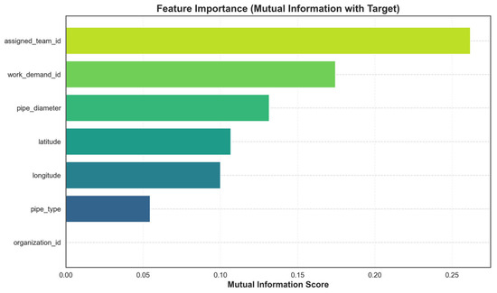
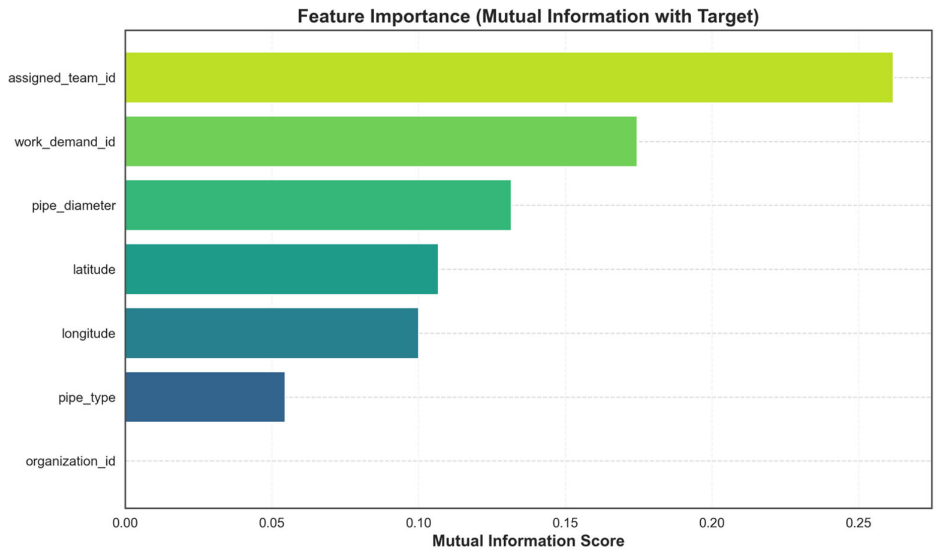
When the graph is examined, it is observed that the first two variables that feed the model the most (reducing entropy the most) are assigned_team_id (0.25+ score) and work_demand_id (~0.17 score). It is also supported by information theory findings that the said variables should be excluded from classification algorithms due to their operational leakage risks despite providing high information gain within this scope (Figure 9).
Figure 9.
Analysis of the predictive power of categorical and numerical features in the wastewater network dataset based on information theory.
3.12. One-Way Analysis of Variance (ANOVA) with Linear Feature Importance and Class Separability
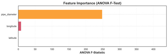
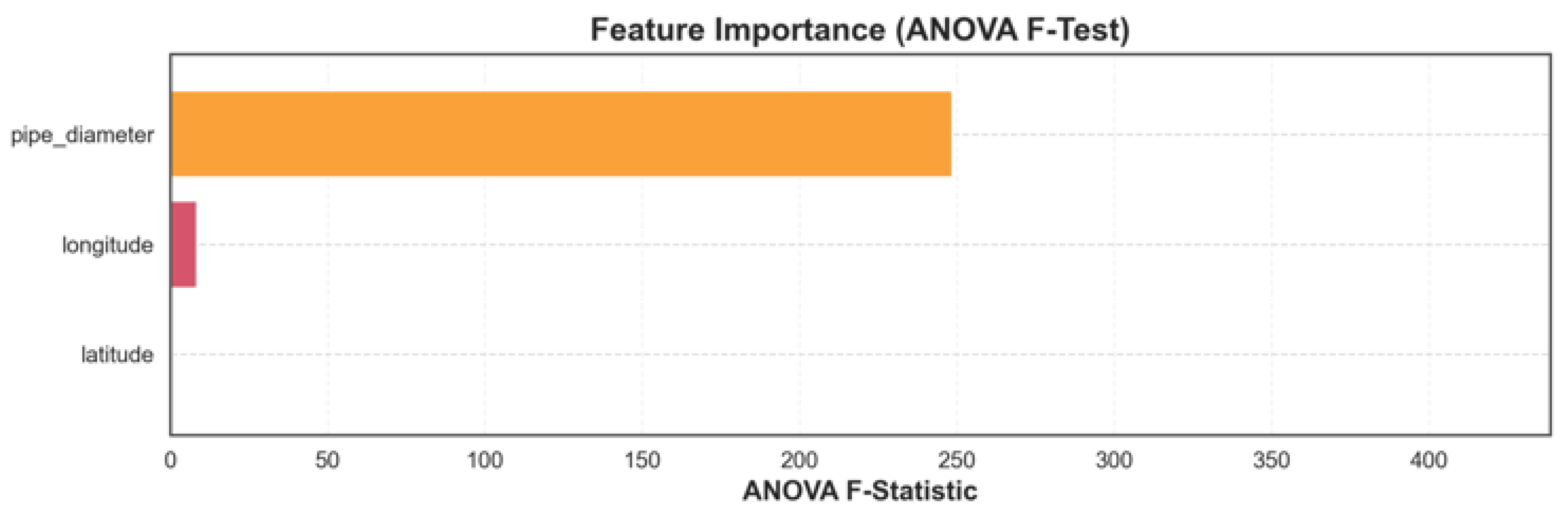
The ANOVA F-Test analysis measures the extent to which the median/mean value of a variable differs (deviates) statistically according to the fault condition by calculating the ratio of the inter-class variance of a variable to the intra-class variance. When examining the graph, it is observed that the variable pipe_diameter (with an F-score of around 250) dominates the dataset in terms of linear separability among continuous features. Nominal identifiers like work_demand_id were excluded from this continuous variance analysis. When the operational variables causing target leakage were cleared from the dataset, it was observed that the pipe_diameter variable stood out as the main parameter of linear separability (Figure 10).
Figure 10.
Feature importance ranking based on one-way ANOVA F-statistic scores measuring the variance differences between the target classes (Class 0: low-priority failure and Class 1: high-priority failure) of the independent variables.
3.13. Discovery of Topological Similarities and Data Islands with T-SNE
T-SNE provides a nonlinear dimensionality reduction approach that preserves local neighborhood relationships, enabling the exploration of underlying patterns in high-dimensional data. The resulting two-dimensional embedding reveals a non-uniform distribution characterized by multiple distinct clusters, or “data islands,” of varying sizes. These patterns suggest the presence of local similarities and potential subgroups within the dataset, offering additional insights into its underlying structure.
3.14. Analysis of Data Compressibility and Linear Independence via Scree Plot
Principal component analysis (PCA) was used to assess the distribution of variance across successive principal components and to evaluate the potential for dimensionality reduction. The first principal component (PC1) explains approximately 28% of the total variance in the dataset, while the second (PC2) and third (PC3) components account for approximately 20% and 14.5%, respectively. These results indicate that the variance is distributed across multiple components rather than being dominated by a single principal component, suggesting that several dimensions are needed to represent the dataset’s variability adequately.
3.15. Severity of the Relationship Between Categorical Attributes and Cramer’s V Analysis
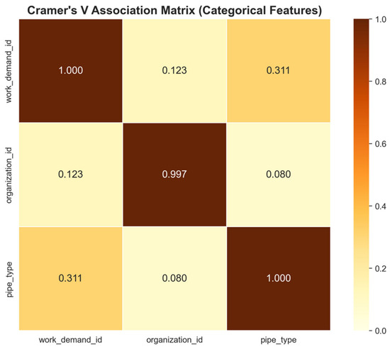
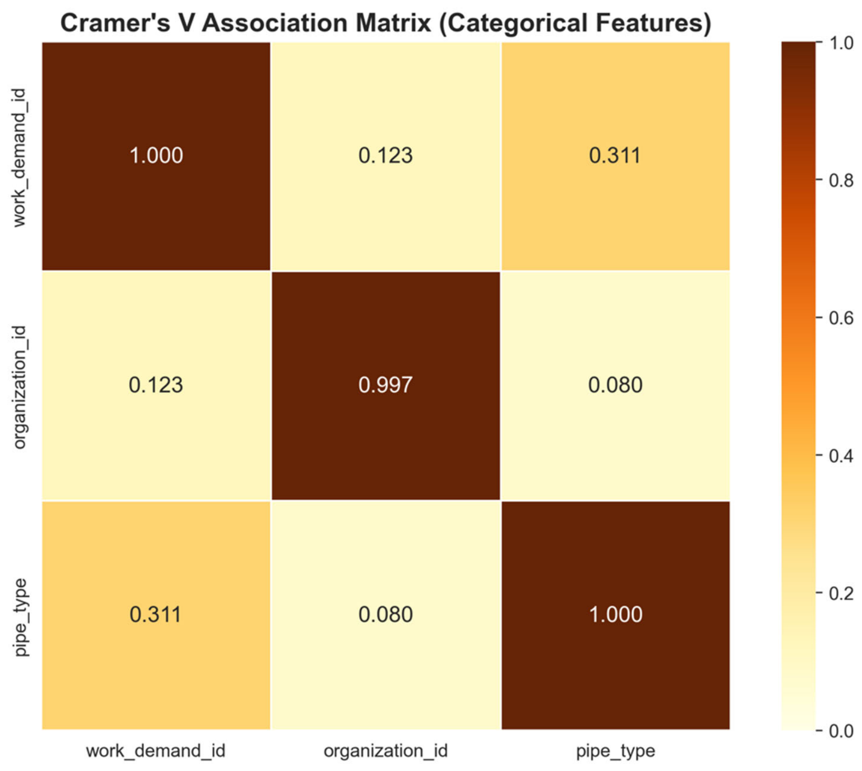
The Chi-square test indicated statistically significant associations among the categorical variables (Figure 11). Cramer’s V was subsequently used to quantify the strength of these associations (Figure 12).
Figure 11.
Heatmap of the p-value from the chi-squared test showing the statistical dependence (interaction) between the primary categorical variables (work_demand_id, organization_id, pipe_type) in the dataset.
Figure 12.
Cramer’s v correlation matrix showing the strength (effect size) of relationships among the basic categorical variables in the dataset, ranging from 0 to 1.
3.16. Performance Analysis of Machine Learning (ML) Models
The test-set (generalization) performance of the machine learning algorithms optimized with hyperparameters using Optuna [31] is presented in Table 2. The classification performances of the algorithms whose hyperparameters were optimized on the training set over the isolated test set were found to be highly competitive. When the findings are examined, it is observed that gradient boosting models achieve the highest success in capturing complex non-linear patterns. Especially, the XGBoost and Gradient Boosting algorithms achieved the highest performance on the dataset. Linear models, on the other hand, have lagged behind tree-based algorithms. Cross-validation mean scores and standard deviations were used to characterize the stability of model performance across data folds. Because no paired significance test or model-to-model confidence-interval comparison was performed, small differences between the leading models were not interpreted as statistically significant superiority. Accordingly, model comparisons are reported on a metric-specific basis rather than by designating a single unequivocally best model. The cross-validation mean scores and their standard deviations (±SD) for F1-Score and AUC-ROC are incorporated into the tables to demonstrate the stability of the models across different data folds.
Table 2.
Performance metrics of machine learning (ML) algorithms on test set and cross-validation stability.
3.17. Deep Learning (DL) Architecture Performances
The test-set performance of the modern deep learning architecture specifically developed for table data is summarized in Table 3. All models were trained using AdamW optimization, a cosine-annealed learning rate, and overfitting-prevention mechanisms. DCN-v2 achieved the highest AUC-ROC among the evaluated deep learning models (0.9251), while Wide & Deep achieved the highest Accuracy (0.8917) and F1-Score (0.8894). The ResNet-Tabular method ranked second with an AUC-ROC score of 0.9242. The AutoInt model, which uses an attention mechanism, has become a strong alternative with an accuracy of 87.08%, while the Wide & Deep method has achieved an accuracy rate of 89.17%, succeeding in tabular data analysis.
Table 3.
Performance metrics of deep learning (DL) algorithms on test set and cross-validation stability.
3.18. Explainability with SHAP Analysis (XAI)
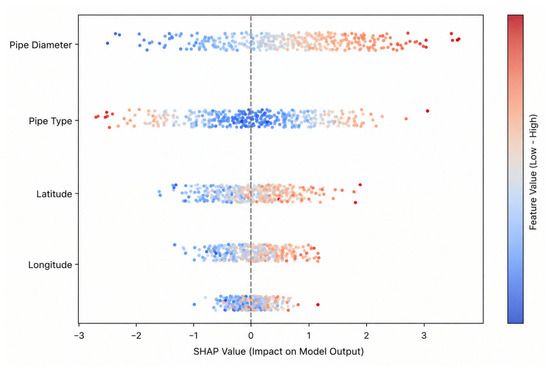
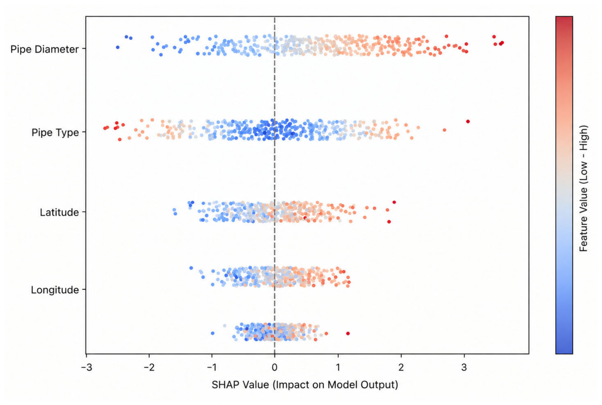
SHAP values were used to quantify the contribution of each feature to the output of the final XGBoost model. Higher pipe diameter values were generally associated with positive SHAP contributions toward Class 1 predictions, indicating that this feature influenced high-priority classifications within the fitted model. These SHAP patterns describe the behavior of the prediction model and should not be interpreted as evidence of a causal relationship or an underlying physical failure mechanism (Figure 13).
Figure 13.
SHAP summary plot for the final XGBoost model illustrating the impact of physical and spatial features on failure risk classification.
An examination of the graph from the presented explainable AI analysis reveals that pipe diameter is the most critical feature shaping the algorithms’ decision-making mechanisms. It is observed that an increase in pipe diameter values directs the model toward the high-priority failure class, whereas small-diameter lines are associated with the low-priority class requiring routine maintenance. It is also evident that pipe type creates a distinct differentiation in risk prioritization. The broad distribution of SHAP values for latitude and longitude indicates that geographic location contributed to the model output in a non-uniform manner. This result should be interpreted as model-level spatial sensitivity rather than direct evidence of causal geographic risk or confirmed spatial hotspots.
3.19. Classification Error Analysis
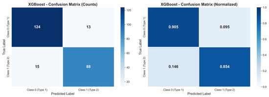
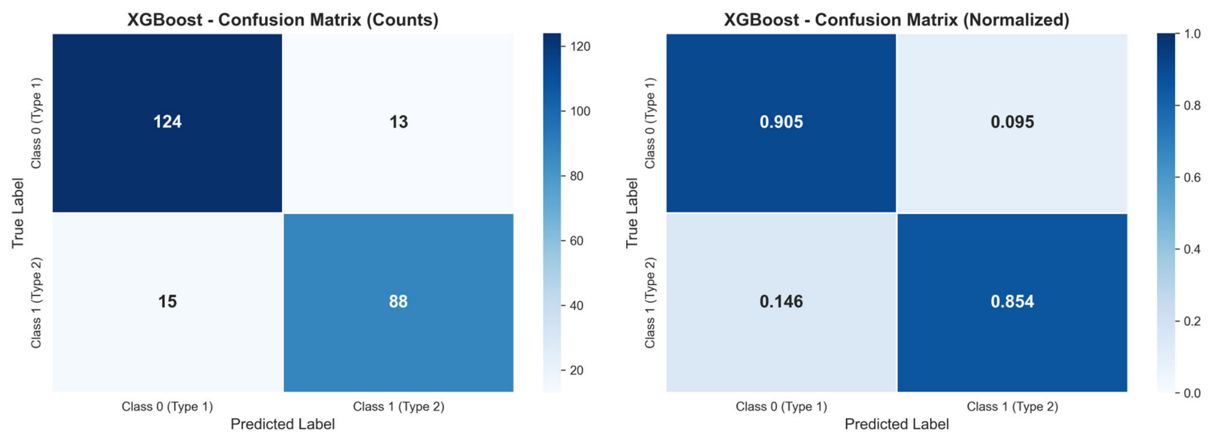
To complement the aggregate performance metrics, the classification errors of the final XGBoost model were evaluated using a confusion matrix on the isolated test set. The false negative rate (FNR) was calculated as FN/(TP + FN), equivalently 1−Sensitivity. For Class 1, the false negative rate was 0.1456 (14.56%), corresponding to a class-specific sensitivity of 0.8544 (85.44%). Thus, 15 of the 103 high-priority failure records in the isolated test set were incorrectly classified as low priority. This metric is particularly relevant for high-priority failures because false negative predictions correspond to urgent cases incorrectly classified as low priority. The confusion matrix and the corresponding FNR are presented in Figure 14.
Figure 14.
XGBoost confusion matrix for Class 0 and Class 1, showing counts and normalized proportions.
4. Conclusions
In tasks such as repair and maintenance, information about how long the work will take can only be accessed through assumptions or past experience. The most important factor in workforce planning is how long the work process will take. On the other hand, it has been determined that identifying the intervention urgency and risk priority of the failure, rather than calculating the exact repair time in operational processes, offers a more applicable logistical planning ground for administrations. In addition, transportation and availability are also important factors. Within the framework of rapidly changing and evolving technology, both public institutions and private-sector organizations are becoming increasingly intertwined with artificial intelligence and integrated systems. Higher-quality service can be made possible with smarter systems. Improving the quality of public services and providing them more quickly, cost-effectively, and appropriately, in accordance with the principles of efficiency and effectiveness, is one of the fundamental duties of both central and local governments.
Therefore, it is necessary to respond to citizens’ requests quickly and effectively. As a result of this analysis, the most effective attributes for the prediction process were identified, and various inferences were drawn from them. The aforementioned inferences have provided meaningful results in terms of both improving service quality and enhancing operational planning. Within the scope of the study, prioritizing maintenance operations based on predictive risk outputs may support proactive planning. System variables carrying target leakage risk were excluded from the analysis, and the field adaptability of the models was increased by preferring the spatial block method in the validation processes. SHAP analysis indicated that pipe diameter and spatial features contributed to the model predictions, without implying causal relationships or underlying physical failure mechanisms.
From an operational perspective, the model outputs may support the prioritization of incoming wastewater failure reports and may contribute to GIS-based decision-support processes. However, the present study did not experimentally evaluate personnel training, equipment stocking, or logistics interventions. These operational topics should therefore be examined in future field-based studies before specific management recommendations are made.
In conclusion, a holistic, data-driven, and proactive fault management approach may support more efficient intervention planning and resource allocation in wastewater networks, thereby contributing to improved public service delivery.
Author Contributions
Conceptualization, M.K.; methodology, M.K.; software, M.K.; validation, M.K. and Ü.H.A.; formal analysis, M.K.; investigation, M.K.; data curation, M.K.; writing—original draft preparation, M.K.; writing—review and editing, Ü.H.A.; visualization, M.K.; supervision, Ü.H.A. All authors have read and agreed to the published version of the manuscript.
Funding
This research received no external funding.
Institutional Review Board Statement
Not applicable.
Informed Consent Statement
Not applicable.
Data Availability Statement
The data that support the findings of this study are available from the corresponding author upon reasonable request.
Acknowledgments
This article was produced as part of a thesis. We would like to thank the Editing Office of the Dean for Research at Erciyes University for the copy-editing and proofreading service for this manuscript.
Conflicts of Interest
The authors declare no conflicts of interest.
Abbreviations
The following abbreviations are used in this manuscript:
| GIS | Geographic Information System |
| KDE | Kernel Density Estimation |
| SVM | Support Vector Machine |
| LDA | Linear Discriminant Analysis |
| K-NN | K-Nearest Neighbors |
| LightGBM | Light Gradient Boosting Machine |
| NLP | Natural Language Processing |
| NODE | Neural Oblivious Decision Ensembles |
| Deep MLP | Deep Multi-Layer Perceptron |
| AutoInt | Automatic Feature Interaction Learning |
| AdaBoost | Adaptive Boosting |
| DL | Deep Learning |
| ML | Machine Learning |
| ANOVA | One-Way Analysis of Variance |
| SHAP | Shapley Additive Explanations |
| XAI | Explainable Artificial Intelligence |
Appendix A. Model Configuration and Hyperparameter Details
Appendix A reports the search spaces, final selected hyperparameters, and architecture settings used in the experiments. For tree-based models, hyperparameter tuning was conducted using the Optuna framework (50 trials) with a fixed random seed (42). For deep learning models, embeddings were utilized for categorical features, and training was guided by early stopping and learning rate scheduling.
Table A1.
Hyperparameter search spaces, final selected values, and architecture configurations for the evaluated models.
References
- Dong, S.; Wang, H.; Mostafizi, A.; Song, X. A network-of-networks percolation analysis of cascading failures in spatially co-located road-sewer infrastructure networks. Phys. A Stat. Mech. Its Appl. 2020, 538, 122971. [Google Scholar] [CrossRef] [Scilit]
- Orhan, C.; Fırat, M. CCTV Kamera Verileri Kullanılarak Atıksu Sistemlerinde Meydana Gelen Arızaların ve Etkili Faktörlerin İncelenmesi. J. Inst. Sci. Technol. Iğdır Üniversitesi Fen Bilim. Enstitüsü Derg. 2020, 10, 2668–2678. [Google Scholar]
- Butler, D.; Digman, C.; Makropoulos, C.; Davies, J.W. Urban Drainage; CRC Press: Boca Raton, FL, USA, 2024. [Google Scholar]
- Ashley, R.M.; Bertrand-Krajewski, J.L.; Hvitved-Jacobsen, T.; Verbanck, M. (Eds.) Solids in Sewers; IWA Publishing: London, UK, 2004. [Google Scholar]
- Mattsson, J.; Hedström, A.; Ashley, R.M.; Viklander, M. Impacts and managerial implications for sewer systems due to recent changes to inputs in domestic wastewater—A review. J. Environ. Manag. 2015, 161, 188–197. [Google Scholar] [CrossRef] [Scilit] [PubMed]
- Murali, M.K.; Hipsey, M.R.; Ghadouani, A.; Yuan, Z. The development and application of improved solids modelling to enable resilient urban sewer networks. J. Environ. Manag. 2019, 240, 219–230. [Google Scholar] [CrossRef] [Scilit] [PubMed]
- Meijer, D.; Van Bijnen, M.; Langeveld, J.; Korving, H.; Post, J.; Clemens, F. Identifying critical elements in sewer networks using graph-theory. Water 2018, 10, 136. [Google Scholar] [CrossRef] [Scilit]
- Fan, X.; Wang, X.; Zhang, X.; Yu, X.B. Machine learning based water pipe failure prediction: The effects of engineering, geology, climate and socio-economic factors. Reliab. Eng. Syst. Saf. 2022, 219, 108185. [Google Scholar] [CrossRef] [Scilit]
- Vucijak, B.; Ceric, A. Multicrtieria prioritization of wastewater projects on example of bihac municipality. Ann. DAAAM Proc. Int. DAAAM Symp. 2011, 22, 933–935. [Google Scholar] [CrossRef] [Scilit]
- Akyürek, H.A. Intelligent Workforce Management by Using Artificial Intelligence Techniques. Master Thesis, Mevlana Üniversitesi, Konya, Türkiye, 2013. [Google Scholar] [CrossRef]
- Çevik, K.K.; Kayakuş, M. İletişim Teknolojileri Departmanında kullanıcıların taleplerine cevap verme süresinin makine öğrenmesi ile tahmin edilmesi. Mühendis. Bilim. VE Tasar. Derg. 2020, 8, 728–739. [Google Scholar]
- Arif, M.; Alghamdi, K.K.; Sahel, S.A.; Alosaimi, S.O.; Alsahaft, M.E.; Alharthi, M.A.; Arif, M. Role of machine learning algorithms in forest fire management: A literature review. J. Robot. Autom. 2021, 5, 212–226. [Google Scholar] [CrossRef] [Scilit] [PubMed]
- Atasever, Ü.H.; Tercan, E. Deep learning-based burned forest areas mapping via Sentinel-2 imagery: A comparative study. Environ. Sci. Pollut. Res. Int. 2024, 31, 5304–5318. [Google Scholar] [CrossRef] [Scilit] [PubMed]
- Atasever, Ü.H.; Bozdağ, A. Carbon footprint mapping of urban areas in Türkiye using hyperparameter-optimized machine learning techniques. Int. J. Environ. Sci. Technol. 2024, 22, 10321–10344. [Google Scholar] [CrossRef] [Scilit]
- Oğuz, M.; Akkurt, Ş. Kayseri ilinin yenilenebilir enerji potansiyeli. Niğde Ömer Halisdemir Üniversitesi Mühendis. Bilim. Derg. 2017, 6, 362–374. [Google Scholar] [CrossRef] [Scilit]
- Paköz, M.Z.; Yaratgan, D.; Şahin, A. Re-mapping urban vitality through Jane Jacobs’ criteria: The case of Kayseri, Turkey. Land Use Policy 2022, 114, 105985. [Google Scholar] [CrossRef] [Scilit]
- Çırağ, B.; Karagöz, R.; Özer, A.E.; Aydın, A.Ö.; Fırat, M. Modelling the dynamic performance of stormwater drainage systems integrated with infiltration trenches. Urban Water J. 2025, 22, 244–257. [Google Scholar] [CrossRef] [Scilit]
- Cheng, H.T.; Koc, L.; Harmsen, J.; Shaked, T.; Chandra, T.; Aradhye, H.; Anderson, G.; Corrado, G.; Chai, W.; Ispir, M.; et al. Wide & deep learning for recommender systems. In Proceedings of the 1st Workshop on Deep Learning for Recommender Systems, Boston, MA, USA, 15 September 2016; pp. 7–10. [Google Scholar]
- Wang, R.; Shivanna, R.; Cheng, D.; Jain, S.; Lin, D.; Hong, L.; Chi, E. DCN V2: Improved deep & cross network and practical lessons for web-scale learning to rank systems. In Proceedings of the Web Conference 2021, Ljubljana, Slovenia, 12–23 April 2021; pp. 1785–1797. [Google Scholar]
- Chen, T.; Guestrin, C. XGBoost: A scalable tree boosting system. In Proceedings of the 22nd Acm Sigkdd International Conference on Knowledge Discovery and Data Mining, San Francisco, CA, USA, 13–17 August 2016; pp. 785–794. [Google Scholar]
- Ke, G.; Meng, Q.; Finley, T.; Wang, T.; Chen, W.; Ma, W.; Ye, Q.; Liu, T.Y. LightGBM: A highly efficient gradient boosting decision tree. Adv. Neural Inf. Process. Syst. 2017, 30, 3146–3154. [Google Scholar]
- Song, W.; Shi, C.; Xiao, Z.; Duan, Z.; Xu, Y.; Zhang, M.; Tang, J. AutoInt: Automatic feature interaction learning via self-attentive neural networks. In Proceedings of the 28th ACM International Conference on Information and Knowledge Management, Beijing, China, 3–7 November 2019; pp. 1161–1170. [Google Scholar]
- Gorishniy, Y.; Rubachev, I.; Khrulkov, V.; Babenko, A. Revisiting deep learning models for tabular data. NeurIPS 2021, 34, 18932–18943. [Google Scholar]
- Yin, G.; Alazzawi, F.J.I.; Bokov, D.; Marhoon, H.A.; El-Shafay, A.S.; Rahman, M.L.; Su, C.H.; Lu, Y.Z.; Nguyen, H.C. Multiple machine learning models for prediction of CO2 solubility in potassium and sodium based amino acid salt solutions. Arab. J. Chem. 2022, 15, 103608. [Google Scholar] [CrossRef] [Scilit]
- Acar, R.; Katipoğlu, O.M.; Çırağ, B. Hybrid VMD-EMD Enhanced Machine Learning Models for Daily Reference Evapotranspiration Forecasting. Eng. Perspect. 2026, 6, 354–373. [Google Scholar] [CrossRef] [Scilit]
- Popov, S.; Morozov, S.; Babenko, A. Neural oblivious decision ensembles for deep learning on tabular data. arXiv 2019, arXiv:1909.06312. [Google Scholar]
- Zendehboudi, A.; Baseer, M.A.; Saidur, R. Application of support vector machine models for forecasting solar and wind energy resources: A review. J. Clean. Prod. 2018, 199, 272–285. [Google Scholar] [CrossRef] [Scilit]
- Raghavendra, S.; Deka, P.C. Support vector machine applications in the field of hydrology: A review. Appl. Soft Comput. 2014, 19, 372–386. [Google Scholar] [CrossRef] [Scilit]
- Çırağ, B.; Bozkurt, C. Multi-scale drought analysis and machine learning-based completion of missing streamflow data in the Aras Basin. Phys. Chem. Earth Parts A/B/C 2026, 144, 104410. [Google Scholar] [CrossRef] [Scilit]
- Vapnik, V.N. The Nature of Statistical Learning Theory; Springer Science& Business Media: Berlin, Germany, 2013. [Google Scholar]
- Akiba, T.; Sano, S.; Yanase, T.; Ohta, T.; Koyama, M. Optuna: A next-generation hyperparameter optimization framework. In Proceedings of the 25th ACM SIGKDD International Conference on Knowledge Discovery & Data Mining, Anchorage, AK, USA, 4–8 August 2019; pp. 2623–2631. [Google Scholar]

Disclaimer/Publisher’s Note: The statements, opinions and data contained in all publications are solely those of the individual author(s) and contributor(s) and not of MDPI and/or the editor(s). MDPI and/or the editor(s) disclaim responsibility for any injury to people or property resulting from any ideas, methods, instructions or products referred to in the content. |
© 2026 by the authors. Licensee MDPI, Basel, Switzerland. This article is an open access article distributed under the terms and conditions of the Creative Commons Attribution (CC BY) license.