Safe and Efficient Trajectory Planning for Unmanned Ground Platforms in Complex Unstructured Environments

Abstract

Irregular, dense, and abruptly varying obstacle distributions complicate local trajectory planning in unstructured environments by imposing stringent safety constraints under limited computational resources. We propose an adaptive rectangular-inflation method that reduces the iterations required by fixed-step safe-corridor construction. A smoothed guide path defines the corridor geometry, and a circumscribed disk conservatively approximates the vehicle footprint. A signed distance field rapidly estimates the clearance between each rectangular boundary and nearby obstacles. The estimated clearances determine both the inflation step and the priority of the four expansion directions. Within the resulting convex corridor, we formulate a Minimum Snap trajectory using differential-flatness-based parameterization and piecewise seventh-degree polynomials. A quadratic program generates the local trajectory subject to continuity, corridor-containment constraints, and derivative bounds. After optimization, a Bézier convex-hull check provides a sufficient condition for continuous corridor containment. Across the two scenarios, adaptive inflation reduced corridor-construction time by 84.55% and 87.21%, respectively, while iteration counts decreased by 90.31% and 89.36%. Comparisons with model predictive control (MPC) and Minimum Acceleration in both scenarios showed smaller jerk variations for Minimum Snap over much of the motion. The method improved corridor-construction efficiency in the evaluated static grid environments while generating local reference trajectories with smooth position, velocity, and acceleration profiles.

1. Introduction

Unmanned ground platforms integrate environmental perception, localization, planning, decision-making, and motion control. Reliable autonomous navigation is therefore central to both mission efficiency and operational safety. Unlike structured roads, unstructured environments lack continuous lane boundaries and regular road geometry, and they often contain complex terrain and obstacle distributions. A planner must consequently account for traversability, safety margins, vehicle dimensions, and motion continuity under limited computational resources. Graph-search, sampling-based, optimization-based, and model-predictive approaches have all been applied to autonomous vehicles and mobile robots. However, jointly achieving safety, computational efficiency, and trajectory executability remains challenging across autonomous-vehicle and mobile-robot planning applications [1,2,3,4,5,6].

Sampling-based methods can search for feasible paths in high-dimensional spaces, but their performance depends on the sampling strategy and implementation parameters [5]. Optimization methods such as Covariant Hamiltonian Optimization for Motion Planning (CHOMP) and Trajectory Optimization (TrajOpt) incorporate trajectory smoothness and collision costs into iterative optimization. They can refine an initial path, but their performance depends on the initialization, collision-cost formulation, and iterative convexification or gradient procedure [7,8]. For road vehicles, Frenet-frame trajectory generation and methods combining state-lattice search with convex optimization can balance search efficiency and trajectory continuity [9,10]. Autonomous-parking and narrow-passage planners commonly use coarse trajectories, Hybrid A-star (A*), or corridor constraints to obtain a feasible initialization before numerical optimal control or nonlinear optimization [11,12,13]. Mining-truck loading and parallel-parking studies have respectively used coarse-to-fine global optimization and safe travel corridors to reduce the difficulty of handling complex vehicle constraints [14,15].

Safe-corridor methods approximate free space with a sequence of connected convex regions. They convert nonconvex collision-avoidance constraints into linear inequalities and provide a structured feasible region for polynomial trajectory optimization. Liu et al. used safe flight corridors to generate dynamically feasible piecewise-polynomial trajectories [16]. Chen et al. investigated online collision-free trajectory generation in unknown cluttered environments [17]. Gao et al. developed online safe planners using the fast marching method, Bernstein basis polynomials, and point-cloud corridors [18,19]. Zhou et al. subsequently improved fast trajectory generation and local replanning efficiency [20,21]. These studies demonstrate the effectiveness of combining convex corridors with polynomial optimization, although most focus on aerial robots. For unmanned ground platforms with finite body dimensions and nonholonomic characteristics, fixed-direction and fixed-step rectangular inflation can cause redundant iterations and repeated collision checks. Signed distance fields (SDFs) provide obstacle-clearance information and support efficient corridor-boundary queries and online planning [18,22]. By contrast, EGO-Planner demonstrates an alternative route in which avoiding full Euclidean signed distance field (ESDF) updates can reduce local-planning cost [21]. Abbati et al. [23] construct overlapping configuration-space axis-aligned bounding boxes (AABBs) through sampling-based exploration and asymmetric binary-search expansion, and optimize spline paths using a linearly constrained quadratic program (LCQP) solved by the Operator Splitting Quadratic Program (OSQP) solver. Their objective combines geometric acceleration and obstacle-clearance terms. In the present method, a smoothed planar guide path supplies the seeds for rectangular inflation, while signed-distance queries determine the expansion step and direction priority. The subsequent optimization minimizes time-domain squared snap subject to continuity, corridor containment, and derivative bounds. Segment-duration updates are followed by coefficient reoptimization, allowing the derivative limits to influence the trajectory geometry.

Safe-space representations also extend beyond discrete chains of convex regions. Arrizabalaga and Ryll [24] use Pythagorean Hodograph curves to incorporate environmental geometry into a spatial planning model and optimize motion within the parameterized free space. Arrizabalaga et al. [25] construct differentiable collision-free corridors using path-parametric off-centered elliptical cross-sections with a polynomial basis, and formulate corridor-volume maximization as a convex problem. These approaches represent the admissible region continuously along a path parameter. The present method instead constructs overlapping rectangular regions through SDF-guided inflation and assigns a time-parameterized polynomial segment to each region.

Differential flatness was introduced by Fliess et al. [26,27]. For a flat system, states and inputs can be expressed using flat outputs and finitely many of their derivatives, providing a basis for trajectory generation and control design. Minimum Snap methods generate high-order smooth trajectories by minimizing the integral of the squared norm of the fourth derivative of position [28,29]. Recent journal studies address differential-flatness-based vehicle trajectory planning [30] and Minimum Snap planning for unmanned surface vehicles [31]. Control barrier functions (CBFs) instead embed safe-set constraints into quadratic programs or model predictive control (MPC) for safety-critical control and dynamic obstacle avoidance [32,33,34]. Safety under uncertain trajectories of other traffic participants can also be addressed within an MPC framework [35]. This study constructs geometrically feasible regions in a static local occupancy grid. Its primary objective is to reduce the computational cost of rectangular inflation while preserving corridor safety and generating a smooth reference trajectory for subsequent tracking control.

The main contributions of this work are summarized as follows:

• We propose an adaptive rectangular-inflation method for constructing safe corridors around a smoothed guide path. The method uses a circumscribed disk to represent the vehicle footprint and a signed distance field (SDF) to determine the step size and priority of each expansion direction, thereby reducing inflation iterations.
• We formulate a Minimum Snap trajectory-planning problem within the resulting convex corridor. Differential-flatness-based parameterization and piecewise seventh-degree polynomials enable the trajectory to be generated through quadratic programming subject to intersegment continuity, corridor-containment constraints, and derivative bounds. A post-solution Bézier convex-hull check provides a sufficient condition for continuous corridor containment.
• We evaluate the proposed method in two static grid environments. The results in both scenarios show substantial reductions in corridor-construction time and iteration count relative to fixed-step inflation, while the generated reference trajectories exhibit smooth position and higher-order derivative profiles. Comparisons with MPC and Minimum Acceleration were performed in both scenarios.

The rest of this paper is structured as follows:

Section 2 describes the construction of the local planning map and the adaptive rectangular-inflation method for safe-corridor generation. Section 3 formulates the Minimum Snap trajectory-planning problem, presents its quadratic-programming solution, and introduces the Bézier-based containment check. Section 4 presents the simulation settings and evaluates corridor-construction efficiency, continuous corridor containment, and trajectory smoothness. Finally, Section 5 concludes the paper.

2. Local Path Planning in Unstructured Environments Using Safe Corridors

2.1. Construction of the Local Planning Map

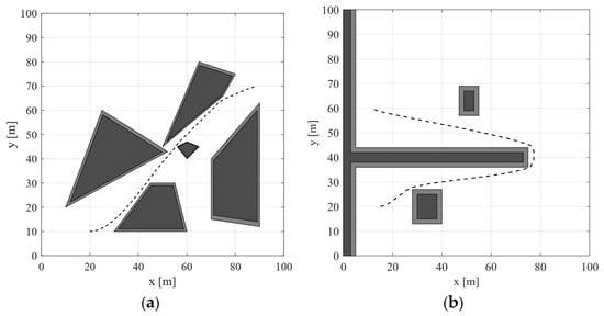
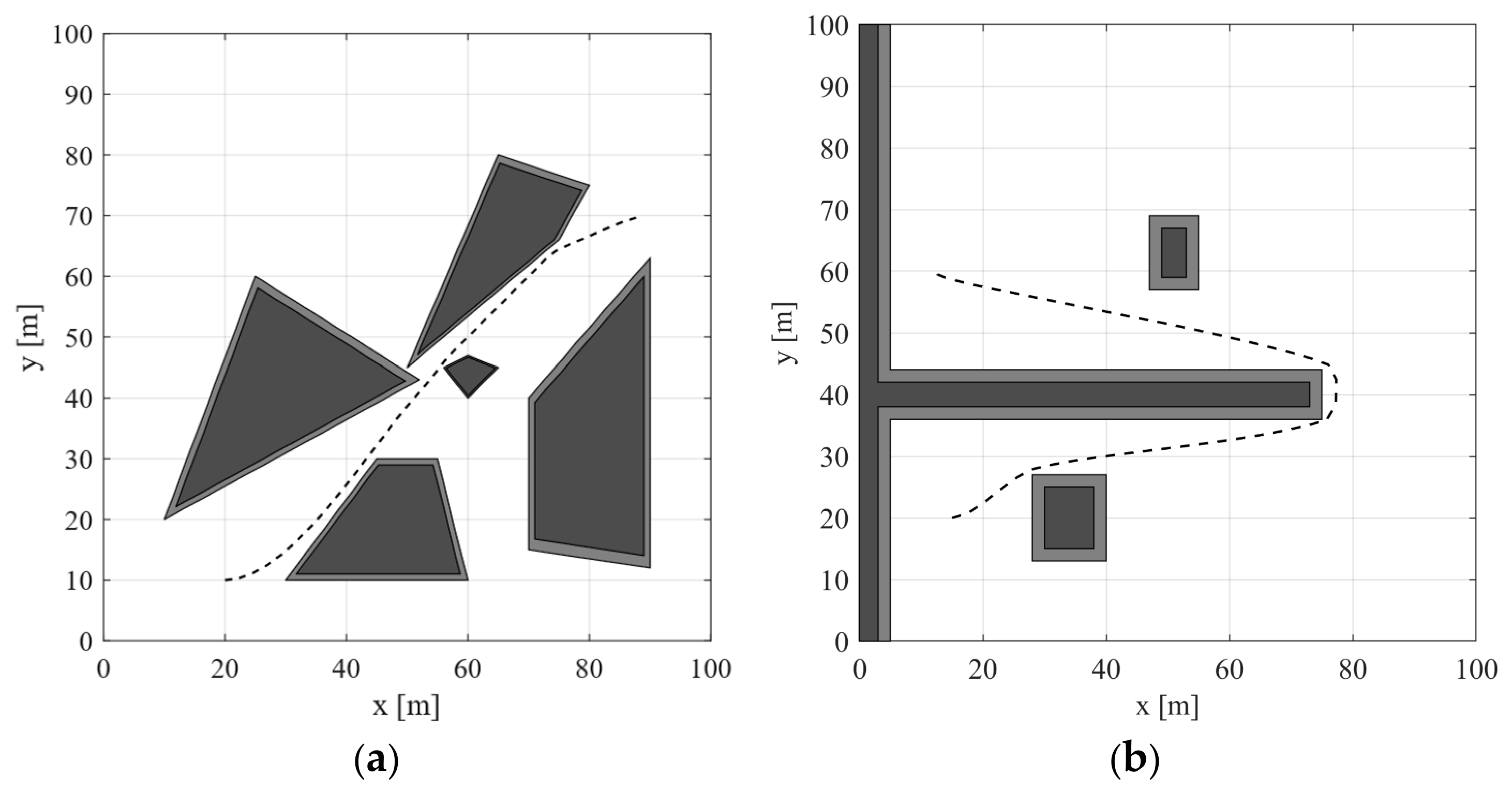
Safe-corridor construction requires a collision-free and sufficiently smooth guide path. This path must connect the local start and target efficiently while providing a stable geometric reference for corridor inflation and trajectory optimization. The rear-axle center of the platform is used as the local starting point, and a look-ahead point on the global path is selected as the target. An improved A* algorithm searches for a discrete path on the binary grid map after obstacle inflation. An adaptive Bézier curve then smooths the path. The resulting sequence of discrete points forms the center guide line for safe-corridor construction after conversion to the circumscribed-disc center using Equation (5). Figure 1 shows the planning environments and guide paths for both scenarios.

Figure 1. Planning environments. (a) Scenario 1; (b) Scenario 2.

Dark regions in the maps denote occupied obstacle regions, while gray borders denote obstacle enlargement. Neither type is traversable. Black curves denote guide paths, which must remain entirely within free space and maintain positive clearance from the inflated obstacle boundary. The platform is a four-wheel ground vehicle with front-wheel steering, whose planar steering geometry is described using a bicycle model. During corridor construction, a circumscribed disk provides a conservative approximation of the vehicle footprint.

2.2. Safe-Corridor Construction Using Adaptive Rectangular Inflation

Let $\mathcal{W}$ denote the two-dimensional workspace and $\mathcal{O}$ the inflated obstacle region. The free space available for local planning is:

$$\mathcal{F}=\mathcal{W}\backslash \mathcal{O}$$

(1)

Given a continuous guide path γ connecting the start and target, the corridor is a sequence of M convex regions C₁,…,C_M. Here, M is the number of corridor elements and associated polynomial segments. The corridor satisfies the following geometric conditions:

• Safety: ${\mathcal{C}}_i\subseteq \mathcal{F}$, meaning that no corridor region intersects the inflated obstacle region.
• Coverage: $\gamma ([0,1])\subseteq {\bigcup }_{i=1}^M{\mathcal{C}}_i$, meaning that the corridor covers the complete guide path.
• Convexity: for any $\mathbf{p},\mathbf{q}\in {\mathcal{C}}_i$ and $\lambda \in [0,1]$, $\lambda \mathbf{p}+(1-\lambda )\mathbf{q}\in {\mathcal{C}}_i$.
• Connectivity: ${\mathcal{C}}_i\cap {\mathcal{C}}_{i+1}\ne \varnothing$, which provides the geometric condition required for continuous transitions between adjacent regions.

Each rectangular corridor element is an AABB. Its boundaries form linear inequalities that can be inserted directly into a quadratic program. Overlap connects neighboring elements geometrically; the trajectory constraints determine whether the prescribed boundary states and derivative bounds can be satisfied within this sequence.

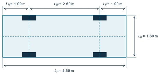
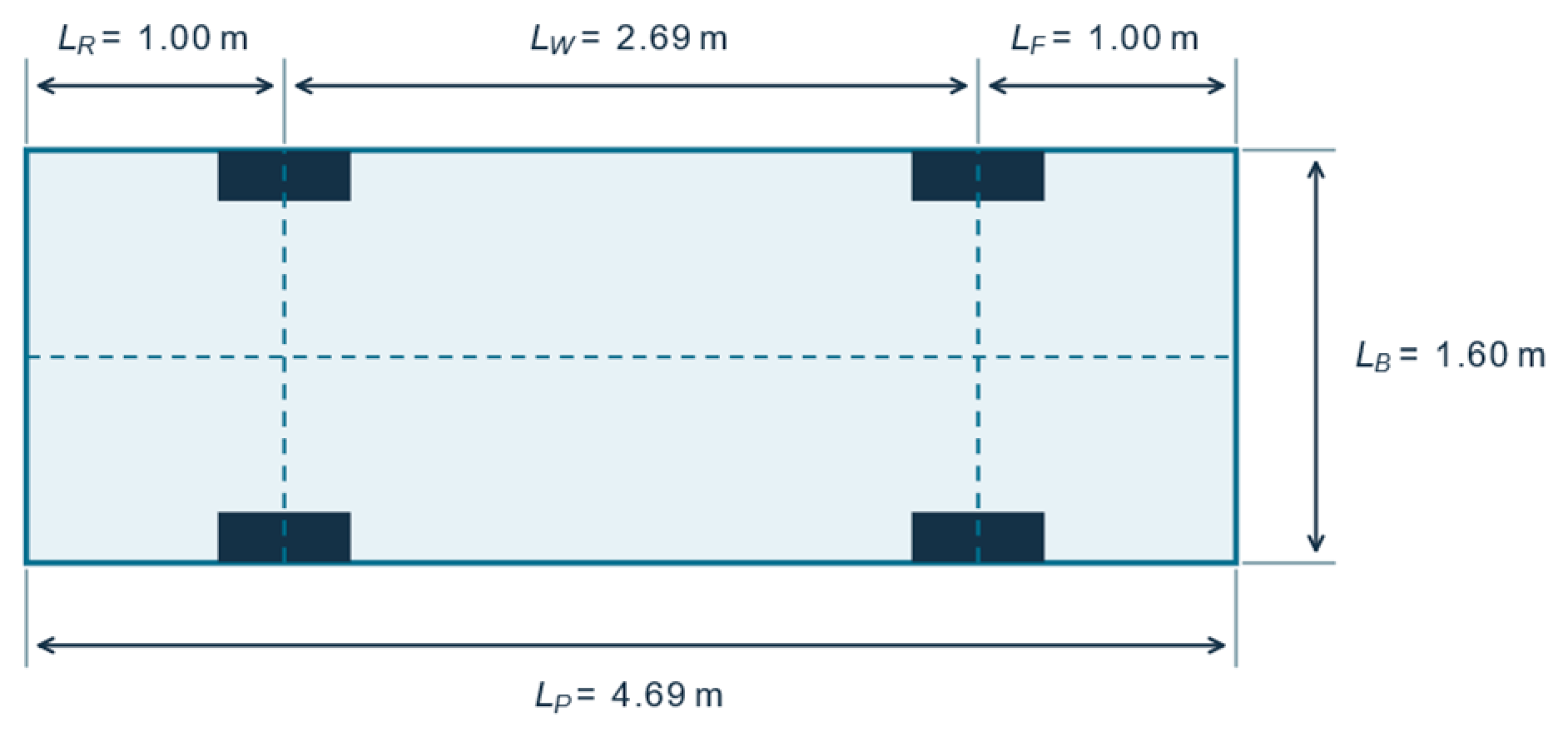
Figure 2 shows the four-wheel vehicle geometry. $L_R$, $L_F$, $L_W$, and $L_B$ denote rear overhang, front overhang, wheelbase, and body width. The vehicle length is:

$$L_P=L_R+L_F+L_W$$

(2)

Figure 2. Vehicle geometry.

The radius of the circumscribed disk centered at the geometric center of the vehicle is:

$$R_v={\displaystyle \frac{1}{2}}\sqrt{L_P^2+L_B^2}$$

(3)

The longitudinal offset from the rear-axle center to the vehicle geometric center is:

$$d_c={\displaystyle \frac{L_F+L_W-L_R}{2}}$$

(4)

If the rear-axle-center coordinates and heading angle at path point $n$ are $(x(n),y(n))$ and $\varphi (n)$, respectively, the disk-center coordinates are:

$$\left\{\begin{array}{c}{x}_c(n)=x(n)+d_c\mathit{cos}\varphi (n)\\ y_c(n)=y(n)+d_c\mathit{sin}\varphi (n)\end{array}\right.$$

(5)

The converted disk centers provide the guide for rectangle inflation. With the occupied obstacle set $O_{\mathrm{o}\mathrm{c}\mathrm{c}}$, the disk-center free space is obtained by excluding the Minkowski sum $O_{\mathrm{o}\mathrm{c}\mathrm{c}}$ ⊕ B($R_v$), with any additional margin included in the obstacle representation. Here, $\mathrm{B}(R_v)$ is the closed disk of radius $R_v$ centered at the origin. This geometric condition connects disk-center clearance to clearance of the enclosed vehicle body. The disk encloses the vehicle body at every orientation. A pose-dependent footprint instead uses orientation-dependent collision checks in configuration space (x,y,$\varphi$).

To avoid searching the entire obstacle set during each expansion, a signed distance field (SDF) stores distance-to-obstacle information for the inflated map [18,22]. For any position $\mathbf{p}$, the signed distance is defined as

$$\Phi (\mathbf{p})=\left\{\begin{array}{c}\underset{\mathbf{q}\in \mathcal{O}}{\min }\Vert \mathbf{p}-\mathbf{q}{\Vert }_2,\mathbf{p}\notin \mathcal{O}\\ -\underset{\mathbf{q}\notin \mathcal{O}}{\min }\Vert \mathbf{p}-\mathbf{q}{\Vert }_2,\mathbf{p}\in \mathcal{O}\end{array}\right.$$

(6)

In Equation (6), $\mathbf{p}$ is the query location and $\mathbf{q}$ is the dummy point over which the nearest-distance minimum is taken. The set containing $\mathbf{q}$ depends on the location of $\mathbf{p}$ relative to the inflated obstacles. The symbol ${\mathbf{p}}_i(t)$ denotes trajectory segment i, and ${\mathbf{q}}_{i,j}$ denotes its jth Bézier control point.

Distances are positive in free space and negative inside the inflated obstacle region. A Euclidean distance transform is precomputed on the grid to obtain a two-dimensional distance array. After this preprocessing step, the distance at any grid location can be queried in $O(1)$ time.

Let the current rectangular boundary be $[x_{min},x_{max}]\times [y_{min},y_{max}]$. Using discrete samples along its boundary, the safe expansion potential in each direction is:

$$\begin{array}{rr}{d}_{left}& =\underset{y\in [y_{\mathit{min}},y_{\mathit{max}}]}{\mathit{min}}\Phi (x_{min},y)\\ d_{right}& =\underset{y\in [y_{\mathit{min}},y_{\mathit{max}}]}{\mathit{min}}\Phi (x_{max},y)\\ d_{down}& =\underset{x\in [x_{\mathit{min}},x_{\mathit{max}}]}{\mathit{min}}\Phi (x,y_{min})\\ d_{up}& =\underset{x\in [x_{\mathit{min}},x_{\mathit{max}}]}{\mathit{min}}\Phi (x,y_{max})\end{array}$$

(7)

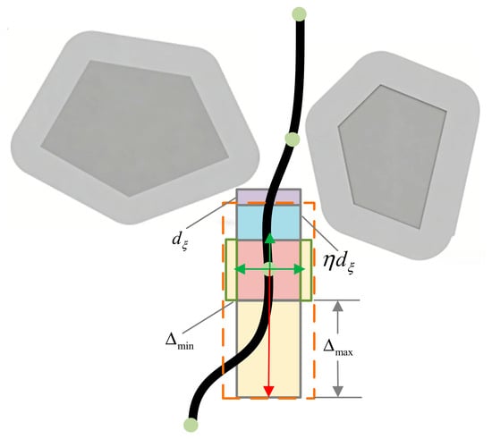
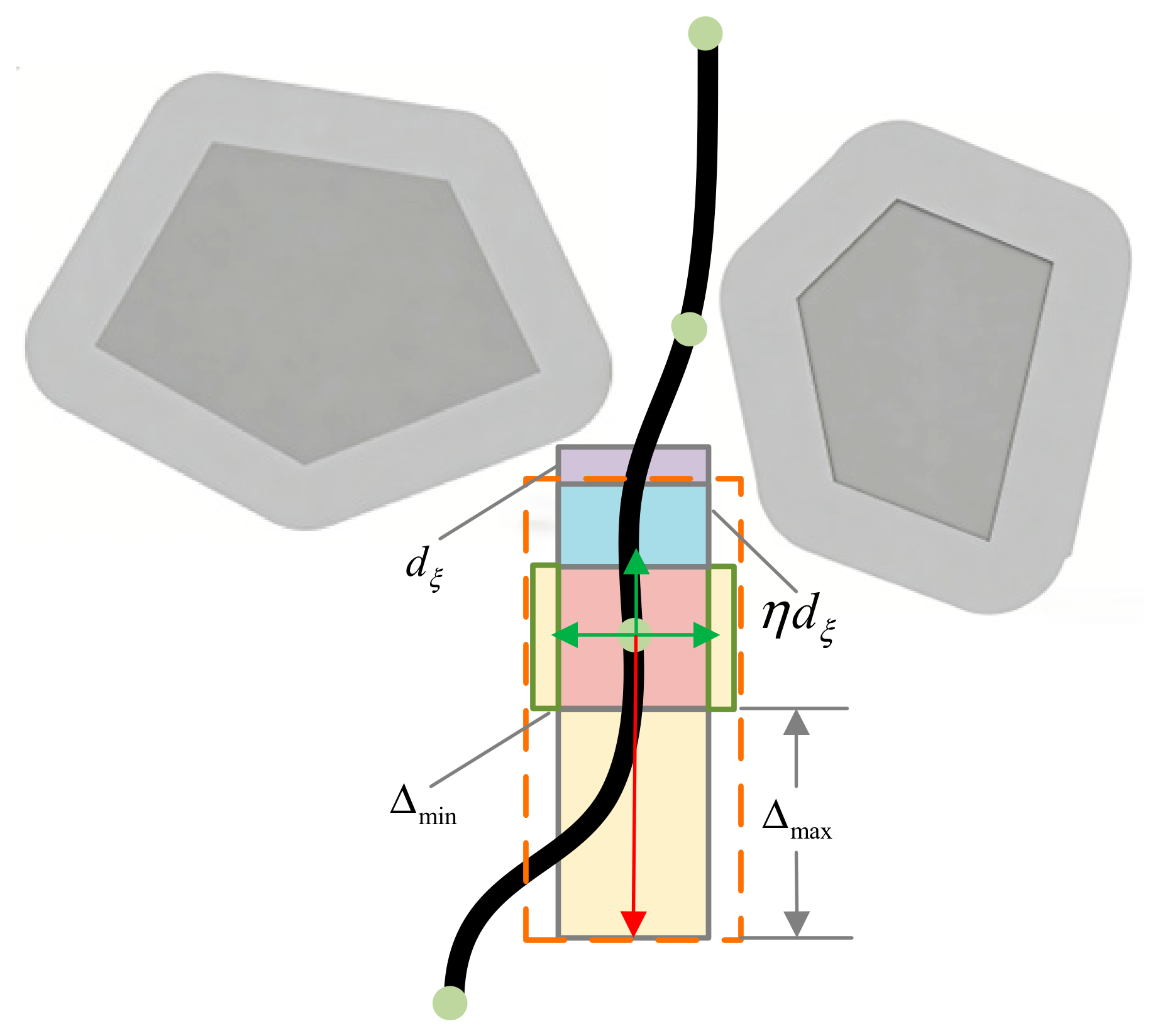
Conventional rectangular inflation typically uses a fixed step size and expansion order. Small steps cause repeated iterations when obstacles are far from the current boundary. A fixed order can also restrict later expansions because earlier updates alter the rectangle geometry. The proposed method defines the expansion potential in each direction as the minimum distance among its boundary samples. It then ranks the directions in descending order of expansion potential. Let $d_{\xi }$ denote the clearance in direction $\xi$. Given the maximum and minimum step sizes ${\Delta }_{max}$ and ${\Delta }_{min}$ and safety coefficient $\eta$, the candidate step is:

$${\Delta }_{\xi }=\mathrm{m}\mathrm{i}\mathrm{n}\left\{{\Delta }_{max},max\left({\Delta }_{min},\eta d_{\xi }\right)\right\}$$

(8)

At the beginning of each inflation round, the four boundary clearances determine the direction order. Each candidate expansion is tested against the inflated obstacle map. A colliding update is retracted, and the affected direction is reduced or stopped. The clearances and order are recomputed for the next round. Inflation stops when no direction can expand further or the prescribed iteration/range limit is reached; overlapping elements are then generated along the guide. In Figure 3, green and red arrows indicate expansion directions; red denotes the greatest expansion potential.

Figure 3. Adaptive rectangular inflation for safe-corridor construction.

3. Minimum Snap Trajectory Planning for an Unmanned Ground Platform

3.1. Formulation of the Minimum Snap Optimization Problem

The safe corridor defines the geometric feasible region, but the time-parameterized trajectory must also satisfy continuity and derivative constraints. We therefore adopt a differential-flatness-based parameterization for a planar integrator-chain planning model. The position $\mathbf{p}(t)=[x(t),y(t){]}^{\mathrm{T}}$ represents the circumscribed-disk center and serves as the flat output. The planning variables are recovered from its derivatives as $\mathbf{v}=\dot{\mathbf{p}}$, $\mathbf{a}=\ddot{\mathbf{p}}$, and $\mathbf{j}={\mathbf{p}}^{(3)}$, where $\mathbf{j}$ is the model input. At nonzero velocity, the trajectory tangent angle is:

$$\varphi (t)=atan2\left(\dot{y}(t),\dot{x}(t)\right)$$

(9)

Here, $\varphi (t)$ denotes the trajectory tangent angle, whereas $\varphi (n)$ in Equation (5) denotes the vehicle heading used for the rear-axle-to-disk-center coordinate conversion. This parameterization converts trajectory smoothness and selected motion constraints into constraints on position and its derivatives, allowing the polynomial coefficients to be optimized directly. The formulation enforces position continuity, higher-order derivative continuity, and their prescribed bounds.

For an additive disturbance $\mathbf{w}(t)$ in the jerk equation, the derivative relation becomes ${\mathbf{p}}^{(3)}=\mathbf{j}+\mathbf{w}$. A known disturbance can be included through $\mathbf{j}={\mathbf{p}}^{(3)}-\mathbf{w}$. The experiments evaluate the generated nominal reference trajectories.

The trajectory is divided into $M$ segments, each associated with a rectangular corridor. Segment $i$ is represented by a seventh-degree polynomial:

$${\mathbf{p}}_i(t)={\sum }_{k=0}^7{\mathbf{c}}_{i,k}{t}^k,\hspace{1em}\hspace{1em}t\in [0,T_i]$$

(10)

Here, ${\mathbf{c}}_{i,k}$ is a two-dimensional polynomial coefficient, $T_i$ is the duration of segment $i$, and $t$ is its local time. Degree seven provides eight coefficients per coordinate for endpoint and junction conditions; the fourth derivative is cubic. For fixed $T_i$, the squared-snap integral is quadratic in the coefficients. Intersegment continuity is enforced by Equation (14). The function ${\mathbf{p}}_i(t)$ denotes segment $i$ of the complete trajectory $\mathbf{p}(t)$, with local time obtained by subtracting the durations of all preceding segments from the global time.

Power and Bernstein bases represent the same seventh-degree polynomial exactly. The power basis makes differentiation and the integral Hessian explicit, while the nonnegative Bernstein functions sum to one and provide the convex-hull property. B-splines offer local support and knot refinement; non-uniform rational B-splines (NURBS) additionally use rational weights.

Trajectory smoothness is promoted by minimizing the sum of the integrals of squared snap over all segments [28,29]:

$$J={\sum }_{i=1}^M{\int }_0^{T_i}{‖{\displaystyle \frac{{\mathrm{d}}^4{\mathbf{p}}_i(t)}{\mathrm{d}{t}^4}}‖}_2^2\mathrm{d}t$$

(11)

After all polynomial coefficients are assembled into $\mathbf{c}$, the objective becomes:

$$J={\displaystyle \frac{1}{2}}{\mathbf{c}}^{\mathrm{T}}\mathbf{Q}\mathbf{c}$$

(12)

where $\mathbf{Q}$ is a positive-semidefinite block-diagonal matrix assembled from the Hessian of each segment. The coefficient subproblem is a convex quadratic program (QP) only when all segment durations $T_i$ are fixed. Optimizing $T_i$ jointly with the polynomial coefficients introduces nonlinear coupling into the objective and constraints.

The initial duration of each segment is estimated from the distance between adjacent guide points and the reference speed $v_{\mathrm{r}\mathrm{e}\mathrm{f}}$:

$$T_i^{(0)}={\displaystyle \frac{\Vert {\mathbf{p}}_{i+1}^g-{\mathbf{p}}_i^g{\Vert }_2}{v_{\mathrm{r}\mathrm{e}\mathrm{f}}}}$$

(13)

In Equation (13), ${{\mathbf{p}}_i}^g$ and ${{\mathbf{p}}_{i+1}}^g$ are guide positions at the beginning and end of segment i; superscript g identifies the guide path. The parameter $v_{\mathrm{r}\mathrm{e}\mathrm{f}}$ is the speed used for this initialization. The polynomial comparisons use a fixed segment duration of $T_i$ = 1 s.

When duration adjustment is required, a violating segment is enlarged according to the largest velocity, acceleration, or jerk ratio, with acceleration and jerk ratios raised to powers 1/2 and 1/3. The coefficients must then be optimized again because the objective and derivative constraints depend on $T_i$. The reoptimization updates the polynomial coefficients within the assigned corridor.

Adjacent trajectory segments satisfy continuity of position, velocity, acceleration, jerk, and snap at each junction:

$${\mathbf{p}}_i^{(r)}(T_i)={\mathbf{p}}_{i+1}^{(r)}(0),\hspace{1em}\hspace{1em}r=0,1,2,3,4$$

(14)

The start, end, and intermediate junction constraints can be assembled as

$${\mathbf{A}}_{\mathrm{e}\mathrm{q}}\mathbf{c}={\mathbf{b}}_{\mathrm{e}\mathrm{q}}$$

(15)

The vector c stacks both coordinate coefficients for all M segments. ${\mathbf{A}}_{\mathrm{e}\mathrm{q}}$ and ${\mathbf{b}}_{\mathrm{e}\mathrm{q}}$ assemble prescribed endpoint conditions and the junction equalities in Equation (14). Their row construction and the corresponding zero junction entries in ${\mathbf{b}}_{\mathrm{e}\mathrm{q}}$ are given explicitly in Appendix A.

The $i$th rectangular safe corridor is represented as

$${\mathcal{C}}_i=\{\mathbf{p}\mid {\mathbf{A}}_i\mathbf{p}\le {\mathbf{b}}_i\}$$

(16)

For the rectangular corridor $C_i=[x_i^{min},x_i^{max}]\times [y_i^{min},y_i^{max}]$, the matrices in Equation (16) can be written as

$${\mathbf{A}}_i=\left[\begin{array}{cc}-1& 0\\ 1& 0\\ 0& -1\\ 0& 1\end{array}\right], {\mathbf{b}}_i=\left[\begin{array}{c}-x_i^{min}\\ x_i^{max}\\ -y_i^{min}\\ y_i^{max}\end{array}\right]$$

The matrix ${\mathbf{A}}_i$ encodes the four outward rectangle normals, and ${\mathbf{b}}_i$ contains the corresponding boundary offsets. The inequality ${\mathbf{A}}_i{\mathbf{p}}_i(t)$≤${\mathbf{b}}_i$ therefore represents the rectangle assigned to segment i.

Trajectory safety requires ${\mathbf{p}}_i(t)\in {\mathcal{C}}_i$. Discrete samples are selected on every trajectory segment. Corridor containment and componentwise bounds on velocity, acceleration, and jerk are imposed at these samples and on the corresponding Bézier control points as linear inequalities:

$${\mathbf{A}}_{\mathrm{i}\mathrm{n}\mathrm{e}\mathrm{q}}\mathbf{c}\le {\mathbf{b}}_{\mathrm{i}\mathrm{n}\mathrm{e}\mathrm{q}}$$

(17)

${\mathbf{A}}_{\mathrm{i}\mathrm{n}\mathrm{e}\mathrm{q}}$ and ${\mathbf{b}}_{\mathrm{i}\mathrm{n}\mathrm{e}\mathrm{q}}$ stack the sampled and control-point corridor rows and the upper and lower componentwise derivative bounds. These rows are linear in c for fixed durations. Appendix A provides their explicit assembly.

If the initial QP is infeasible, the current planning run terminates without outputting a trajectory. After the quadratic program is solved, Equation (22) converts each segment to Bézier control points. Equation (23) is a sufficient continuous-containment criterion for its assigned rectangle. If any segment fails the containment test, midpoints are inserted between its existing constraint samples and the QP is solved again, keeping the safe corridors, segment durations, objective, and other constraints unchanged. The resulting trajectory is then checked again using Equation (23). If the re-solved QP is infeasible or any segment still fails the containment test, the candidate trajectory is rejected and the current planning run terminates without outputting a trajectory.

3.2. Quadratic-Programming Solution and Trajectory Generation

For fixed segment durations, the trajectory problem is an LCQP:

$$\begin{array}{cc}\hfill \underset{\mathbf{c}}{\min }& {\displaystyle \frac{1}{2}}{\mathbf{c}}^{\mathrm{T}}\mathbf{Q}\mathbf{c}\hfill \\ \hfill \mathrm{s}.\mathrm{t}.& {\mathbf{A}}_{\mathrm{e}\mathrm{q}}\mathbf{c}={\mathbf{b}}_{\mathrm{e}\mathrm{q}},\hfill \\ & {\mathbf{A}}_{\mathrm{i}\mathrm{n}\mathrm{e}\mathrm{q}}\mathbf{c}\le {\mathbf{b}}_{\mathrm{i}\mathrm{n}\mathrm{e}\mathrm{q}}.\hfill \end{array}$$

(18)

Because $\mathbf{Q}$ is positive semidefinite, the fixed-time coefficient subproblem is a convex quadratic program. The OSQP solver, which is based on the alternating direction method of multipliers, solves the problem while exploiting matrix sparsity [36].

After the coefficients have been obtained, the global time determines the active segment. Its position and derivatives are evaluated as

$${\mathbf{p}}_i^{(r)}(t)={\displaystyle \frac{{\mathrm{d}}^r}{\mathrm{d}{t}^r}}\left({\sum }_{k=0}^7{\mathbf{c}}_{i,k}{t}^k\right),\hspace{1em}\hspace{1em}r=0,1,2,3$$

(19)

The derivative orders r = 0, 1, 2, 3 give position, velocity, acceleration, and jerk. They define the local reference trajectory at a selected sampling period.

To verify that the continuous curve remains within the corridor, segment $i$ is converted from the power basis to the Bernstein basis:

$${\mathbf{p}}_i(t)={\sum }_{j=0}^7{\mathbf{q}}_{i,j}{B}_{j,7}\left({\displaystyle \frac{t}{T_i}}\right)$$

(20)

$$B_{j,7}(\tau )=\left({\displaystyle \genfrac{}{}{0pt}{}{7}{j}}\right){\tau }^j(1-\tau {)}^{7-j},\hspace{1em}\hspace{1em}\tau \in [0,1]$$

(21)

where ${\mathbf{q}}_{i,j}$ is a Bézier control point. The normalized segment time is $\tau =t/T_i$. For the power-basis coefficients ${\mathbf{c}}_{i,k}$, the control points are obtained through the linear transformation

$${\mathbf{q}}_{i,j}={\sum }_{k=0}^j{\displaystyle \frac{\left(\genfrac{}{}{0pt}{}{j}{k}\right)}{\left(\genfrac{}{}{0pt}{}{7}{k}\right)}}{T}_i^k{\mathbf{c}}_{i,k},\hspace{1em}\hspace{1em}j=0,1,\dots ,7$$

(22)

In Equation (22), ${T_i}^k$ is the kth power of the duration of segment i. Indices j and k identify a Bézier control point and a power-basis coefficient. Both ${\mathbf{q}}_{i,j}$ and ${\mathbf{c}}_{i,k}$ are two-dimensional vectors.

A Bézier curve lies entirely within the convex hull of its control points. Therefore, the entire segment is contained in its assigned corridor if all position control points satisfy

$${\mathbf{A}}_i{\mathbf{q}}_{i,j}\le {\mathbf{b}}_i,\hspace{1em}\hspace{1em}j=0,1,\dots ,7$$

(23)

Certification of the piecewise trajectory requires this test for every segment. The same condition is imposed in Equation (18) as linear coefficient constraints through Equation (22) for fixed durations. Algorithm 1 summarizes the procedure.

Algorithm 1. Corridor construction, trajectory optimization, and containment test
Step	Operation
Input	Inflated occupancy map; disk-center guide; inflation and trajectory parameters.
1	Precompute the SDF and initialize a rectangle around a guide point.
2	Query boundary samples, rank the four clearances, and propose steps using Equation (8).
3	Test candidate updates; retract colliding expansions. Repeat until the stop criterion is met.
4	Continue along the guide with overlapping rectangles and assign one polynomial segment to each element.
5	Fix the current segment durations; assemble the objective, continuity, sampled, and control-point constraints; solve Equation (18). If durations are adjusted, reassemble and solve the QP again. If the initial QP is infeasible, reject the candidate and terminate the planning run.
6	Convert coefficients using Equation (22); evaluate Equation (23) for every assigned rectangle. If any segment fails, insert midpoints between its constraint samples, re-solve Equation (18) once, and repeat the containment test.
Output	Output position and derivative references only if all segments pass. Otherwise, or if the re-solved QP is infeasible, reject the trajectory and terminate the planning run.

For fixed durations, derivative control points depend linearly on position control points. Componentwise bounds on velocity, acceleration, and jerk control points are imposed in Equation (18) to enforce continuous derivative limits while preserving the LCQP structure [37].

4. Simulation Results and Analysis

The evaluation contains two parts. The maps in Figure 4 and Figure 5 provide fixed-step versus adaptive-inflation benchmarks. The comparison plots evaluate Minimum Snap, an MPC planner, and Minimum Acceleration in a polygonal-obstacle layout and a U-turn obstacle-avoidance layout. The three planners have different trajectory completion times.

4.1. Safe-Corridor Construction and Trajectory-Planning Results

The simulations were implemented in MATLAB R2021b on a Lenovo computer equipped with a 12th-generation Intel Core i7-12700H processor (14 cores), 16 GB LPDDR5 memory (4800 MHz), and an NVIDIA GeForce RTX 2050 GPU (4 GB). In the inflation benchmark, simulated lidar data were projected and binarized into a 9000 × 8000 occupancy grid, with a 10% obstacle enlargement. Figure 4, Figure 5, Figure 6, Figure 7, Figure 8, Figure 9, Figure 10 and Figure 11 present the safe corridors, signed distance fields, and trajectory comparisons. Map coordinates are expressed in meters. Table 1 lists the disk-approximation, polynomial, and fixed-step settings. Table 2 lists the vehicle-model parameters.

Table 1. Disk approximation, polynomial settings, and fixed-step baseline parameters.

Quantity	Value
Circumscribed-disk radius $R_v$	2.478 m
Rear-axle to disk-center offset $d_c$	1.345 m
Polynomial degree	7
Number of trajectory segments, $M$	Scenario 1: 34; Scenario 2: 47
Coefficients per coordinate	8 per segment
Comparison segment duration $T_i$	1 s
Fixed-step rectangle initialization	0.02 m up/down, 0.03 m left/right
Fixed-step increment	0.01 m
Maximum inflation rounds	700
Fixed-step direction order	left → down → right → up
Reference speed	20 km/h

Table 1. Disk approximation, polynomial settings, and fixed-step baseline parameters.

Quantity	Value
Circumscribed-disk radius $R_v$	2.478 m
Rear-axle to disk-center offset $d_c$	1.345 m
Polynomial degree	7
Number of trajectory segments, $M$	Scenario 1: 34; Scenario 2: 47
Coefficients per coordinate	8 per segment
Comparison segment duration $T_i$	1 s
Fixed-step rectangle initialization	0.02 m up/down, 0.03 m left/right
Fixed-step increment	0.01 m
Maximum inflation rounds	700
Fixed-step direction order	left → down → right → up
Reference speed	20 km/h

Table 2. Vehicle-model parameters.

Quantity	Value
Speed interval	0–6.5 m/s
Longitudinal acceleration	−2.5 to 1.8 m/s2
Longitudinal jerk	−2.5 to 2.5 m/s3
Longitudinal snap	−4 to 4 m/s4
Front-wheel steering angle	±30°
Steering-angle rate	±55°/s
Lateral acceleration	±2.8 m/s2
Steering first-order time constant	0.27 s

Table 2. Vehicle-model parameters.

Quantity	Value
Speed interval	0–6.5 m/s
Longitudinal acceleration	−2.5 to 1.8 m/s2
Longitudinal jerk	−2.5 to 2.5 m/s3
Longitudinal snap	−4 to 4 m/s4
Front-wheel steering angle	±30°
Steering-angle rate	±55°/s
Lateral acceleration	±2.8 m/s2
Steering first-order time constant	0.27 s

The quantities in Table 2 are vehicle-frame or steering-model values. The planar LCQP constrains Cartesian position derivatives, as specified in Appendix A; the steering-angle and steering-rate values in Table 2 describe the vehicle model. The MPC planner uses a vehicle kinematic model and outputs speed, snap, and steering-angle rate. Its objective combines penalties on output magnitudes with target-approach and obstacle-distance terms. Minimum Snap and Minimum Acceleration use the same safe corridors, segment durations, and constraints, differing only in the optimization objective.

Scenario 1 contains several polygonal obstacles and a constrained transition near the map center. Scenario 2 requires a U-turn around the right end of a long horizontal obstruction, with additional obstacles on the outgoing and returning branches. Blue denotes Minimum Snap, green denotes MPC, and orange denotes Minimum Acceleration. The black dashed line is the guide, and blue rectangles are the corridor elements.

Figure 4. Safe corridor and trajectory comparison. (a) Scenario 1; (b) Scenario 2.

Figure 4. Safe corridor and trajectory comparison. (a) Scenario 1; (b) Scenario 2.

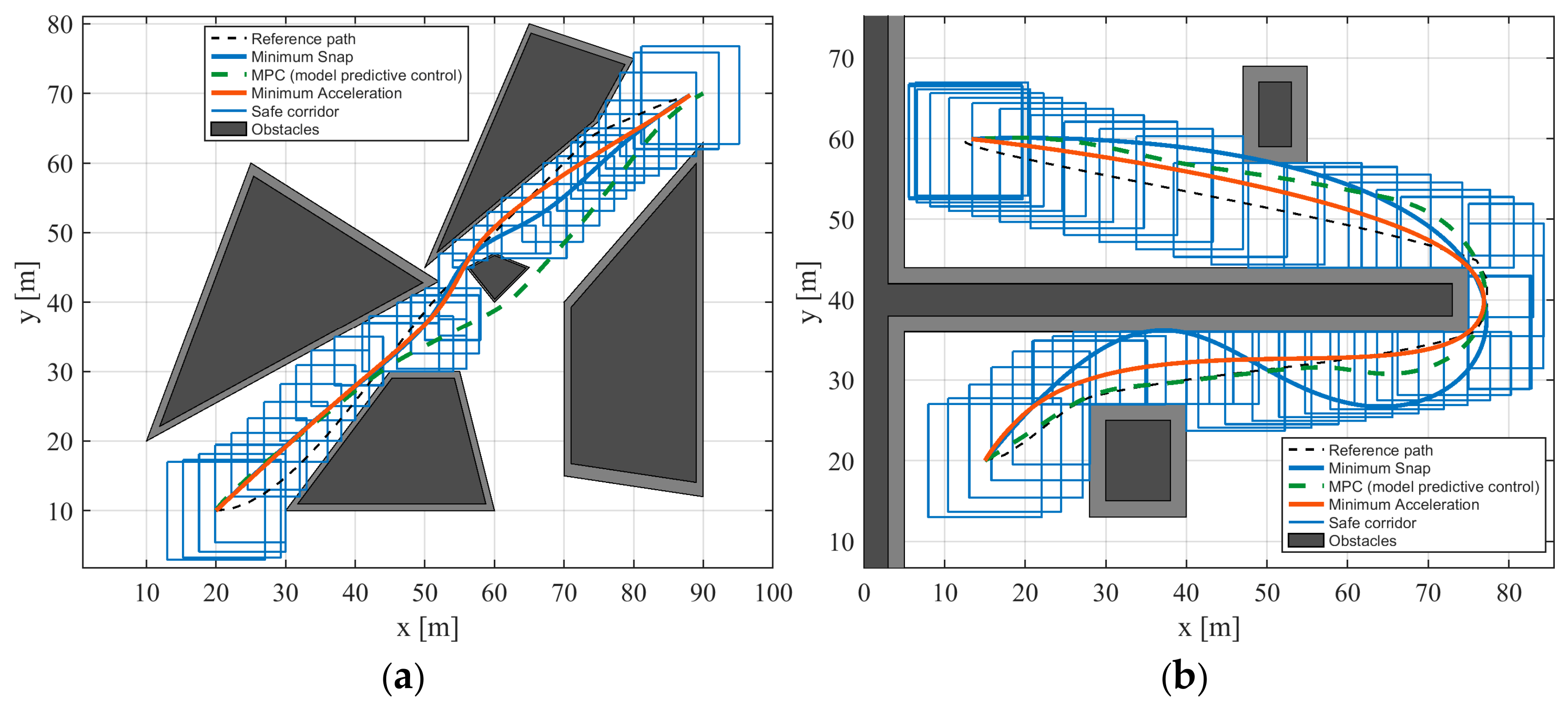
Figure 4a shows how the three planners traverse the polygonal-obstacle layout. The generated rectangles were distributed continuously along the guide path, with overlap between adjacent rectangles providing a connected sequence of convex feasible regions. Near the central obstacles, the available clearance restricted rectangular expansion, whereas the rectangles extended farther in open regions. Minimum Snap and Minimum Acceleration followed similar overall routes within the displayed corridor coverage, whereas the MPC path differed near the lower obstacles and the central transition.

Figure 4b shows the U-turn obstacle-avoidance layout. The outward and return branches are separated by a long obstruction, so the trajectory must pass its right end before returning toward the goal. The corridor elements followed both branches and overlapped around the turn, providing connected feasible regions through the change in direction. The three trajectories passed around the obstruction, but differed along the lower branch: Minimum Snap formed a more pronounced rise and subsequent descent, Minimum Acceleration followed a flatter course, and MPC lay lower over much of this branch.

4.2. Performance of Adaptive Rectangular Inflation

Figure 5 shows the signed distance fields for the two comparison maps. The surface height and color represent the signed distance in meters. Positive values indicate free space and negative values indicate the interior of the obstacle representation. Larger positive distances indicate more available expansion space. The algorithm queries the rectangular boundaries to determine the expansion potential in each direction, uses larger candidate steps in open directions, and reduces the step near obstacles. The SDF therefore provides a common measure for both adaptive step selection and directional prioritization.

Figure 5. Signed distance fields in the two scenarios. (a) Scenario 1; (b) Scenario 2.

Figure 5. Signed distance fields in the two scenarios. (a) Scenario 1; (b) Scenario 2.

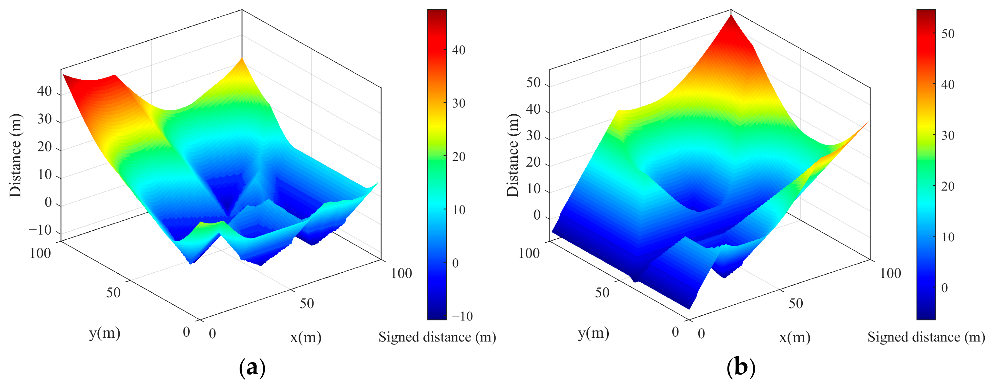
Table 3 and Table 4 report the measured inflation results for Scenario 1 and Scenario 2, respectively.

Table 3. Rectangular-inflation comparison in Scenario 1.

Construction Method	Construction Time (ms)	Iterations	Time Reduction (%)	Speedup
Fixed-step inflation	69.9416	2290	—	1.00
Adaptive rectangular inflation	10.8084	222	84.55	6.47

Table 3. Rectangular-inflation comparison in Scenario 1.

Construction Method	Construction Time (ms)	Iterations	Time Reduction (%)	Speedup
Fixed-step inflation	69.9416	2290	—	1.00
Adaptive rectangular inflation	10.8084	222	84.55	6.47

Table 4. Rectangular-inflation comparison in Scenario 2.

Construction Method	Construction Time (ms)	Iterations	Time Reduction (%)	Speedup
Fixed-step inflation	87.3949	3290	—	1.00
Adaptive rectangular inflation	11.1785	350	87.21	7.82

Table 4. Rectangular-inflation comparison in Scenario 2.

Construction Method	Construction Time (ms)	Iterations	Time Reduction (%)	Speedup
Fixed-step inflation	87.3949	3290	—	1.00
Adaptive rectangular inflation	11.1785	350	87.21	7.82

In Scenario 1, adaptive inflation reduced corridor-construction time from 69.9416 to 10.8084 ms, a reduction of 84.55%. The iteration count decreased from 2290 to 222, a reduction of 90.31%. In Scenario 2, construction time decreased from 87.3949 to 11.1785 ms, a reduction of 87.21%, while the iteration count decreased from 3290 to 350, a reduction of 89.36%. These results correspond to speedups of 6.47 and 7.82, respectively.

The fixed-step baseline requires repeated small expansions even when substantial clearance is available. Adaptive inflation instead uses the boundary-clearance estimates to make larger updates in open directions, while dynamic directional priority changes the order of expansion as the rectangle grows.

If the map contains $N$ cells, the preprocessing complexity of the Euclidean distance field is $O(N)$. Suppose corridor rectangle $i$ undergoes $K_i$ inflation iterations and queries P_i boundary samples per iteration. After the distance field has been constructed, the inflation-query cost is approximately

$$T_{\mathrm{e}\mathrm{x}\mathrm{p}\mathrm{a}\mathrm{n}\mathrm{d}}=O\left({\sum }_{i=1}^M{K}_i{P}_i\right)$$

(24)

The expression accounts for rectangle count, inflation rounds, and boundary queries after SDF preprocessing. The adaptive step directly affects the number of rounds, while the boundary-sampling interval affects the number of queries per round. Dynamic ordering prioritizes directions with greater available clearance and can reduce ineffective expansion attempts.

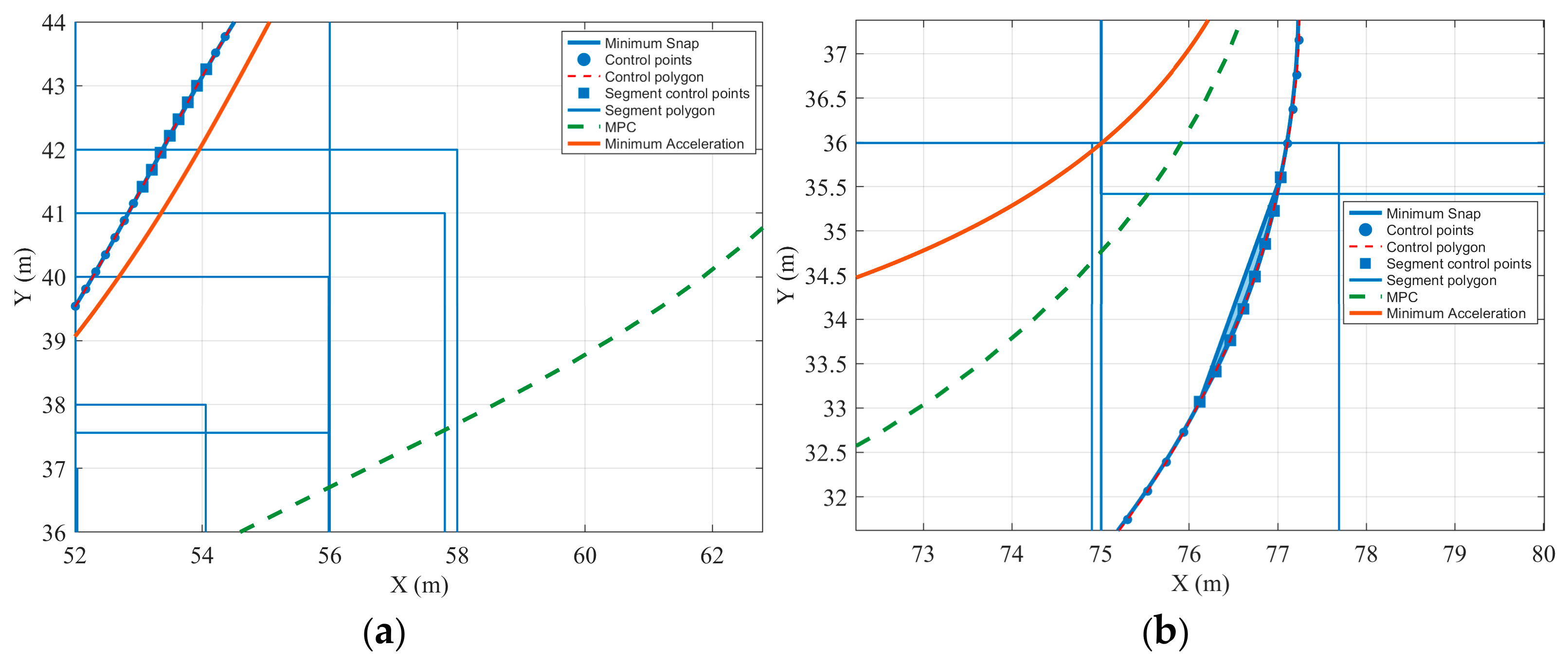
To examine continuous-time corridor containment, each optimized seventh-degree polynomial is converted to the equivalent Bézier representation. Figure 6 shows representative curve portions, their control points, and the nearby corridor elements in both scenarios. The control points expose the geometry used for the convex-hull test: when all control points of a segment lie in its assigned rectangle, the complete segment lies in that rectangle by the Bézier convex-hull property. The criterion in Equation (23) is applied to the rectangle assigned to each segment.

Figure 6. Verification of safe-corridor containment. (a) Scenario 1; (b) Scenario 2.

Figure 6. Verification of safe-corridor containment. (a) Scenario 1; (b) Scenario 2.

4.3. Comparison of the Trajectory-Planning Methods

Figure 7 compares the planar outputs of Minimum Snap, MPC, and Minimum Acceleration. In Scenario 1, the two polynomial trajectories followed similar routes, while MPC took a lower course through the central transition before approaching the same target region. In Scenario 2, all three trajectories completed the turn, but their return branches differed: Minimum Snap showed a rise followed by a descent, whereas Minimum Acceleration followed a flatter course. The trajectory samples on the Minimum Snap curves also illustrate the continuous connection of the piecewise representation. Minimum Acceleration minimizes the integral of the squared norm of the second position derivative, whereas Minimum Snap penalizes the fourth derivative.

Figure 7. Comparison of planar trajectories. (a) Scenario 1; (b) Scenario 2.

Figure 7. Comparison of planar trajectories. (a) Scenario 1; (b) Scenario 2.

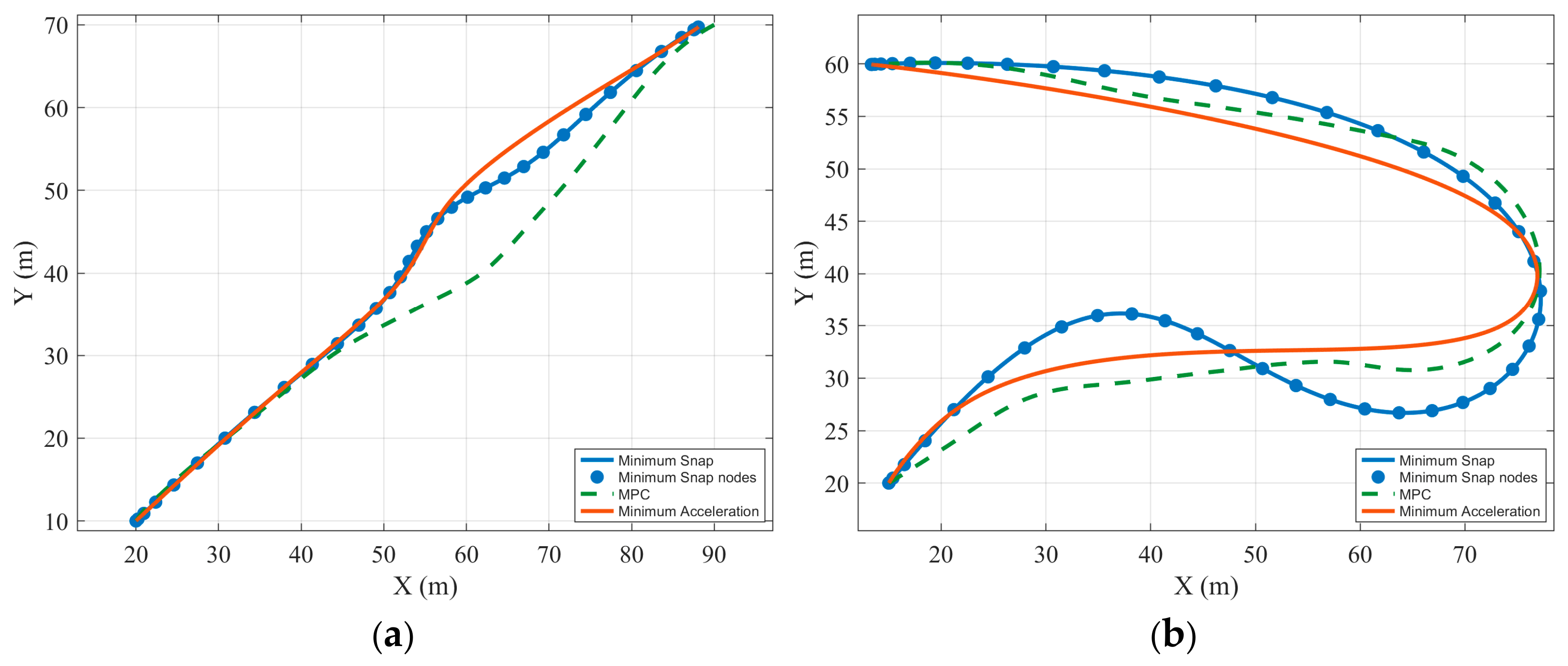
Figure 8 shows $x(t)$ and y(t) over time. The Minimum Snap position components remained continuous throughout both scenarios, with no visible positional jumps between polynomial segments. In Scenario 1, both components increased toward the target. In Scenario 2, $x(t)$ first increased and then decreased, corresponding to the outward and return motion around the obstruction, while the changes in y(t) reflected the separation between the two branches. The MPC histories ended earlier than the polynomial histories in both, whereas Minimum Snap and Minimum Acceleration had similar completion times.

Figure 8. Comparison of position components. (a) Scenario 1; (b) Scenario 2.

Figure 8. Comparison of position components. (a) Scenario 1; (b) Scenario 2.

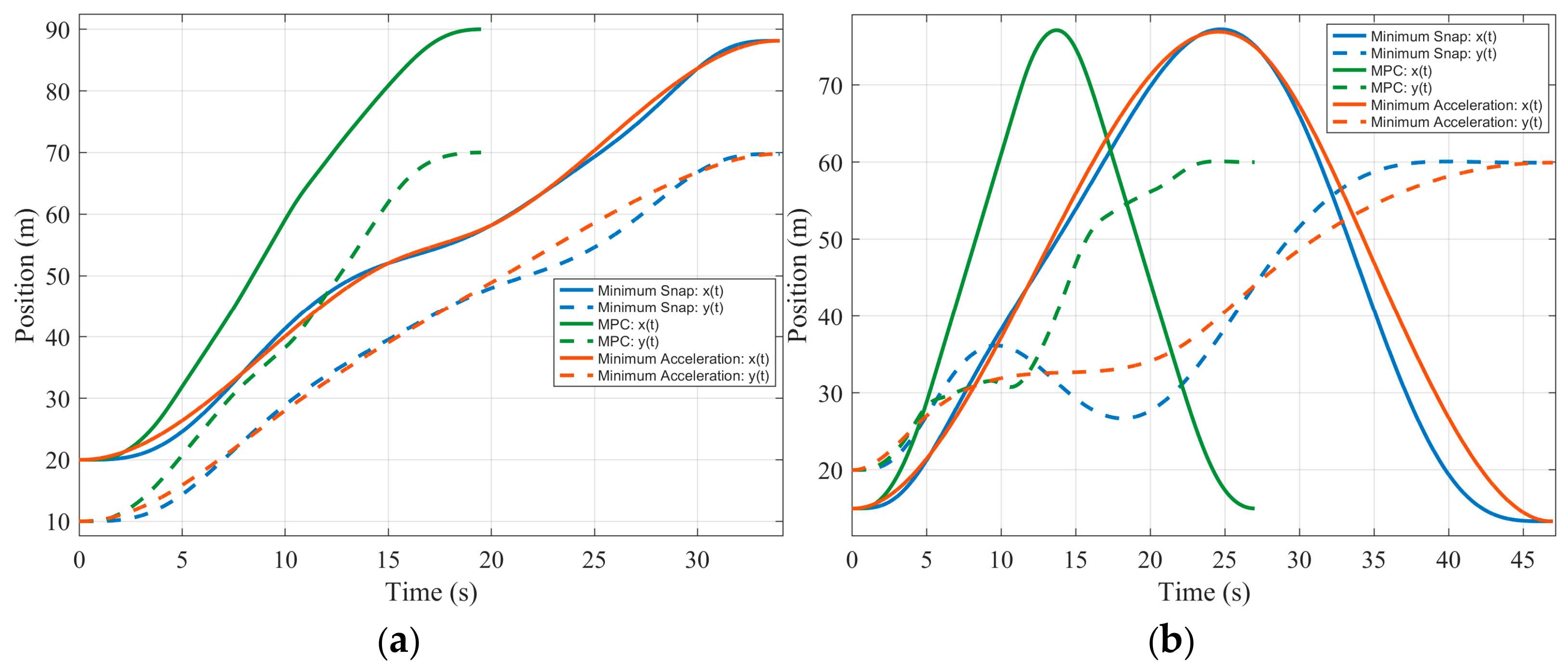
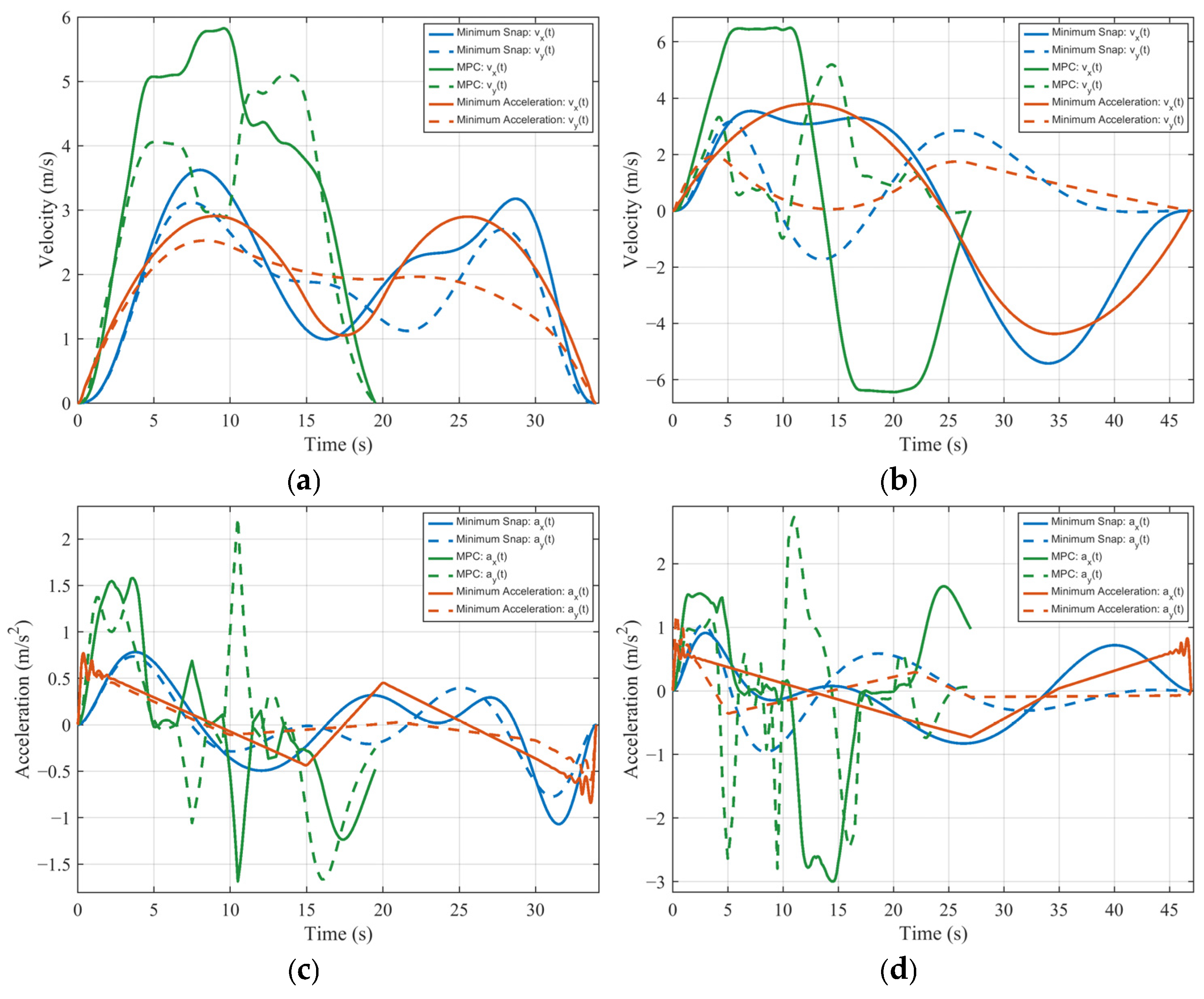
Figure 9 compares velocity and acceleration components. In Scenario 1, the Minimum Snap velocities varied continuously and decreased toward zero at the end of the trajectory. MPC reached higher velocity levels over a shorter interval and exhibited sharper changes during acceleration and deceleration. In Scenario 2, the x-velocity changed from positive to negative as the platform reversed its direction of travel. Minimum Snap and Minimum Acceleration made this transition gradually, whereas MPC showed a faster transition between approximately constant positive and negative velocity levels. The acceleration plots further distinguish the methods: Minimum Snap varied smoothly over most of the motion, while MPC showed larger and more frequent changes and Minimum Acceleration showed sharper variations near the terminal stage.

Figure 9. Comparison of velocity and acceleration components. (a,b) Velocity components in Scenarios 1 and 2, respectively; (c,d) acceleration components in Scenarios 1 and 2, respectively.

Figure 9. Comparison of velocity and acceleration components. (a,b) Velocity components in Scenarios 1 and 2, respectively; (c,d) acceleration components in Scenarios 1 and 2, respectively.

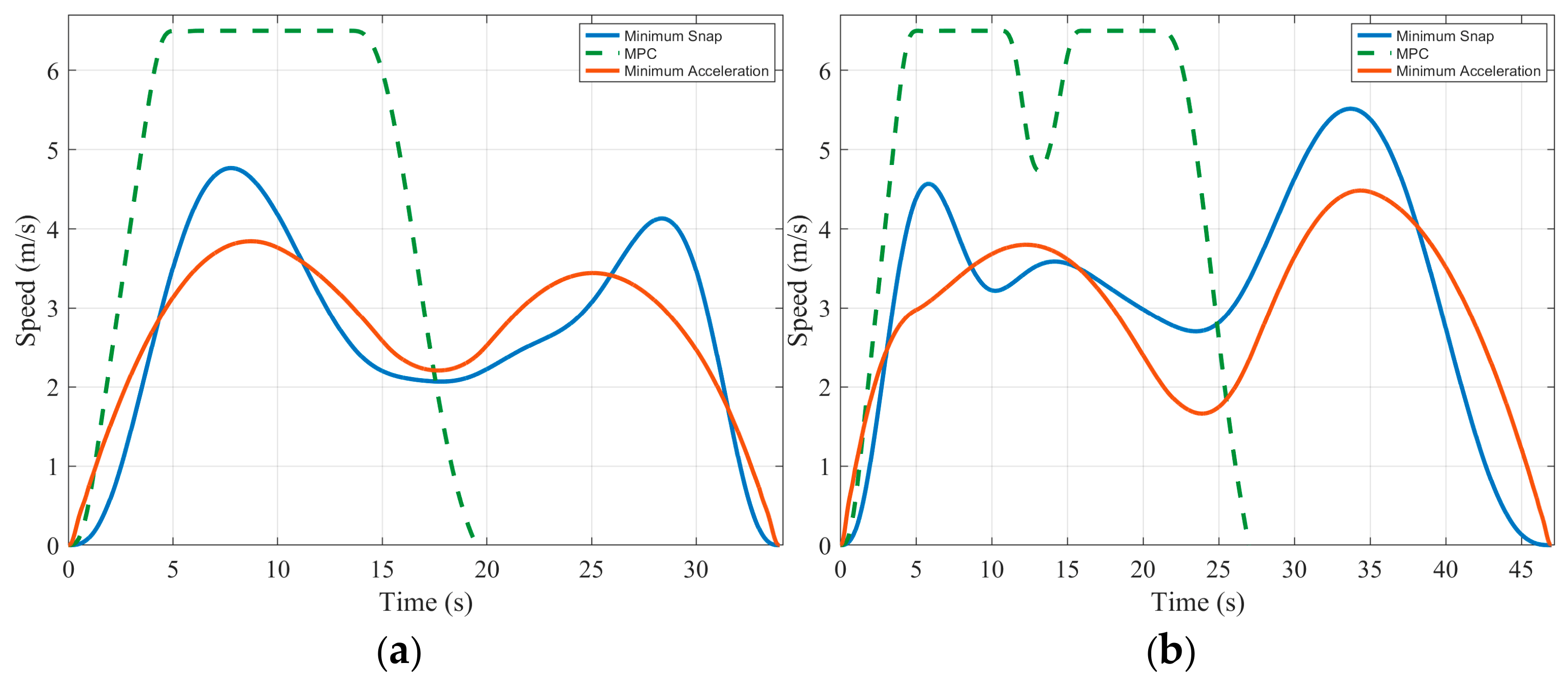
The resultant speed is computed from the two Cartesian velocity components as

$$v(t)=\sqrt{{\dot{x}}^2(t)+{\dot{y}}^2(t)}$$

(25)

The resultant-speed profiles in Figure 10 combine the two Cartesian velocity components and therefore reflect both the spatial trajectory and its time allocation. In Scenario 1, the two polynomial methods showed an increase, an intermediate decrease, and a second increase before decelerating to the endpoint. In Scenario 2, their speed decreased around the direction reversal and increased again along the return branch. Minimum Snap maintained a continuous speed profile through these transitions. MPC exhibited higher, approximately constant speed levels over parts of each trajectory and sharper transitions over its shorter completion interval.

Figure 10. Comparison of resultant speed. (a) Scenario 1; (b) Scenario 2.

Figure 10. Comparison of resultant speed. (a) Scenario 1; (b) Scenario 2.

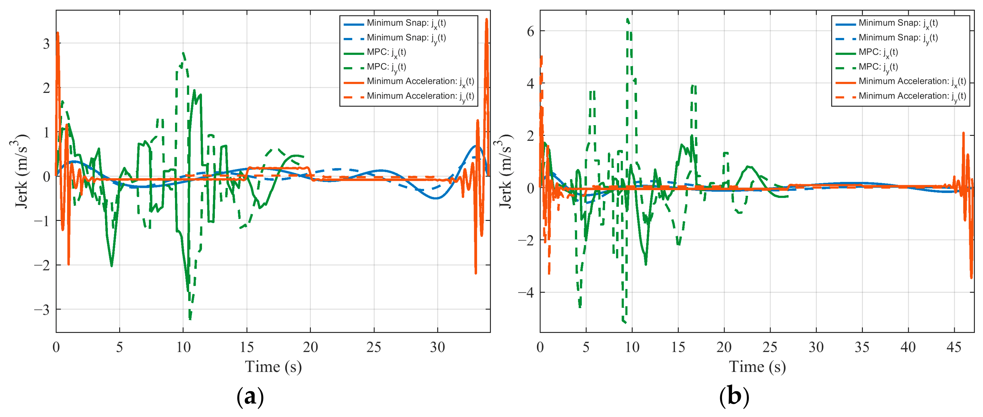
Jerk measures the rate of change in acceleration and reveals higher-order variations that are less apparent in the position plots. Figure 11 shows that Minimum Snap had smaller jerk variations over much of the displayed motion in both scenarios. Minimum Acceleration exhibited pronounced variations near the start and end, despite its comparatively smooth position profiles, while MPC showed repeated sharper changes during its shorter motion interval. Minimum Snap minimizes the integral of the squared norm of the fourth position derivative, whereas the junction equalities enforce intersegment jerk continuity.

Figure 11. Comparison of jerk components. (a) Scenario 1; (b) Scenario 2.

Figure 11. Comparison of jerk components. (a) Scenario 1; (b) Scenario 2.

5. Conclusions

This study developed a local trajectory-planning method that combines adaptive safe-corridor inflation with Minimum Snap optimization. A circumscribed disk represents the vehicle footprint, while an SDF estimates the expansion potential at each rectangular boundary. Adaptive step sizes and dynamic directional priorities then construct connected convex corridors. Within these corridors, piecewise seventh-degree polynomials represent the position trajectory. For fixed segment durations, a convex quadratic program imposes intersegment continuity, corridor-containment constraints, and componentwise derivative bounds. A post-solution Bézier convex-hull check evaluates continuous corridor containment.

In two simulated scenarios, the method reduced corridor-construction time by 84.55% and 87.21% and reduced iteration counts by 90.31% and 89.36%, respectively. Comparisons with MPC and Minimum Acceleration showed smaller jerk variations for Minimum Snap over much of the displayed motion. The planner generated position, velocity, acceleration, and jerk reference profiles with intersegment continuity. Future work will investigate flatness-based trajectory tracking for the vehicle model, accounting for the rear-axle-to-disk-center transformation. Feedforward longitudinal and steering commands could be combined with tracking-error feedback to compensate for disturbances while respecting actuator limits.

References

- Yurtsever, E.; Lambert, J.; Carballo, A.; Takeda, K. A survey of autonomous driving: Common practices and emerging technologies. IEEE Access 2020, 8, 58443–58469. [Google Scholar] [CrossRef] [Scilit]
- Paden, B.; Čáp, M.; Yong, S.Z.; Yershov, D.; Frazzoli, E. A survey of motion planning and control techniques for self-driving urban vehicles. IEEE Trans. Intell. Veh. 2016, 1, 33–55. [Google Scholar] [CrossRef] [Scilit]
- Schwarting, W.; Alonso-Mora, J.; Rus, D. Planning and decision-making for autonomous vehicles. Annu. Rev. Control Robot. Auton. Syst. 2018, 1, 187–210. [Google Scholar] [CrossRef] [Scilit]
- Reda, M.; Onsy, A.; Haikal, A.Y.; Ghanbari, A. Path planning algorithms in the autonomous driving system: A comprehensive review. Robot. Auton. Syst. 2024, 174, 104630. [Google Scholar] [CrossRef] [Scilit]
- Elbanhawi, M.; Simic, M. Sampling-based robot motion planning: A review. IEEE Access 2014, 2, 56–77. [Google Scholar] [CrossRef] [Scilit]
- Hoy, M.; Matveev, A.S.; Savkin, A.V. Algorithms for collision-free navigation of mobile robots in complex cluttered environments: A survey. Robotica 2015, 33, 463–497. [Google Scholar] [CrossRef] [Scilit]
- Ratliff, N.; Zucker, M.; Bagnell, J.A.; Srinivasa, S. CHOMP: Gradient optimization techniques for efficient motion planning. In Proceedings of the 2009 IEEE International Conference on Robotics and Automation, Kobe, Japan, 12–17 May 2009; pp. 489–494. [Google Scholar]
- Schulman, J.; Duan, Y.; Ho, J.; Lee, A.; Awwal, I.; Bradlow, H.; Pan, J.; Patil, S.; Goldberg, K.; Abbeel, P. Motion planning with sequential convex optimization and convex collision checking. Int. J. Robot. Res. 2014, 33, 1251–1270. [Google Scholar] [CrossRef] [Scilit]
- Werling, M.; Ziegler, J.; Kammel, S.; Thrun, S. Optimal trajectory generation for dynamic street scenarios in a Frenet frame. In Proceedings of the 2010 IEEE International Conference on Robotics and Automation, Anchorage, AK, USA, 3–7 May 2010; pp. 987–993. [Google Scholar]
- Meng, Y.; Wu, Y.; Gu, Q.; Liu, L. A decoupled trajectory planning framework based on the integration of lattice searching and convex optimization. IEEE Access 2019, 7, 130530–130551. [Google Scholar] [CrossRef] [Scilit]
- Li, B.; Acarman, T.; Zhang, Y.; Ouyang, Y.; Yaman, C.; Kong, Q.; Zhong, X.; Peng, X. Optimization-based trajectory planning for autonomous parking with irregularly placed obstacles: A lightweight iterative framework. IEEE Trans. Intell. Transp. Syst. 2022, 23, 11970–11981. [Google Scholar] [CrossRef] [Scilit]
- Sheng, W.; Li, B.; Zhong, X. Autonomous parking trajectory planning with tiny passages: A combination of multistage Hybrid A-Star algorithm and numerical optimal control. IEEE Access 2021, 9, 102801–102810. [Google Scholar] [CrossRef] [Scilit]
- Lian, J.; Ren, W.; Yang, D.; Li, L.; Yu, F. Trajectory planning for autonomous valet parking in narrow environments with enhanced Hybrid A* search and nonlinear optimization. IEEE Trans. Intell. Veh. 2023, 8, 3723–3734. [Google Scholar] [CrossRef] [Scilit]
- Li, B.; Ouyang, Y.; Li, X.; Cao, D.; Zhang, T.; Wang, Y. Mixed-integer and conditional trajectory planning for an autonomous mining truck in loading/dumping scenarios: A global optimization approach. IEEE Trans. Intell. Veh. 2023, 8, 1512–1522. [Google Scholar] [CrossRef] [Scilit]
- Jin, X.; Tao, Y.; Opinat Ikiela, N.V. Trajectory planning design for parallel parking of autonomous ground vehicles with improved safe travel corridor. Symmetry 2024, 16, 1129. [Google Scholar] [CrossRef] [Scilit]
- Liu, S.; Watterson, M.; Mohta, K.; Sun, K.; Bhattacharya, S.; Taylor, C.J.; Kumar, V. Planning dynamically feasible trajectories for quadrotors using safe flight corridors in 3-D complex environments. IEEE Robot. Autom. Lett. 2017, 2, 1688–1695. [Google Scholar] [CrossRef] [Scilit]
- Chen, J.; Liu, T.; Shen, S. Online generation of collision-free trajectories for quadrotor flight in unknown cluttered environments. In Proceedings of the 2016 IEEE International Conference on Robotics and Automation, Stockholm, Sweden, 16–21 May 2016; pp. 1476–1483. [Google Scholar]
- Gao, F.; Wu, W.; Lin, Y.; Shen, S. Online safe trajectory generation for quadrotors using fast marching method and Bernstein basis polynomial. In Proceedings of the 2018 IEEE International Conference on Robotics and Automation, Brisbane, Australia, 21–25 May 2018; pp. 344–351. [Google Scholar]
- Gao, F.; Wu, W.; Gao, W.; Shen, S. Flying on point clouds: Online trajectory generation and autonomous navigation for quadrotors in cluttered environments. J. Field Robot. 2019, 36, 710–733. [Google Scholar] [CrossRef] [Scilit]
- Zhou, B.; Gao, F.; Wang, L.; Liu, C.; Shen, S. Robust and efficient quadrotor trajectory generation for fast autonomous flight. IEEE Robot. Autom. Lett. 2019, 4, 3529–3536. [Google Scholar] [CrossRef] [Scilit]
- Zhou, X.; Wang, Z.; Ye, H.; Xu, C.; Gao, F. EGO-Planner: An ESDF-free gradient-based local planner for quadrotors. IEEE Robot. Autom. Lett. 2021, 6, 478–485. [Google Scholar] [CrossRef] [Scilit]
- Pan, Y.; Kompis, Y.; Bartolomei, L.; Mascaro, R.; Stachniss, C.; Chli, M. Voxfield: Non-projective signed distance fields for online planning and 3D reconstruction. In Proceedings of the 2022 IEEE/RSJ International Conference on Intelligent Robots and Systems, Kyoto, Japan, 23–27 October 2022; pp. 5331–5338. [Google Scholar]
- Abbati, R.; Riboli, M.; Rosselli, M.; Tasora, A.; Silvestri, M. A General Approach to Path Planning Within C-Space Safe Corridors. IEEE Robot. Autom. Lett. 2026, 11, 578–585. [Google Scholar] [CrossRef] [Scilit]
- Arrizabalaga, J.; Ryll, M. Spatial motion planning with Pythagorean Hodograph curves. In Proceedings of the 2022 IEEE 61st Conference on Decision and Control, Cancun, Mexico, 6–9 December 2022; pp. 2047–2053. [Google Scholar]
- Arrizabalaga, J.; Manchester, Z.; Ryll, M. Differentiable Collision-Free Parametric Corridors. In Proceedings of the 2024 IEEE/RSJ International Conference on Intelligent Robots and Systems, Abu Dhabi, United Arab Emirates, 14–18 October 2024; pp. 1839–1846. [Google Scholar]
- Fliess, M.; Lévine, J.; Martin, P.; Rouchon, P. Sur les systèmes non linéaires différentiellement plats. C. R. Acad. Sci. Paris 1992, 315, 619–624. [Google Scholar]
- Fliess, M.; Lévine, J.; Martin, P.; Rouchon, P. Flatness and defect of non-linear systems: Introductory theory and examples. Int. J. Control 1995, 61, 1327–1361. [Google Scholar] [CrossRef] [Scilit]
- Mellinger, D.; Kumar, V. Minimum snap trajectory generation and control for quadrotors. In Proceedings of the 2011 IEEE International Conference on Robotics and Automation, Shanghai, China, 9–13 May 2011; pp. 2520–2525. [Google Scholar]
- Singh, B.K.; Kumar, A. Attitude and position control with minimum snap trajectory planning for quadrotor UAV. Int. J. Dyn. Control 2023, 11, 2342–2353. [Google Scholar] [CrossRef] [Scilit]
- Han, Z.; Wu, Y.; Li, T.; Zhang, L.; Pei, L.; Xu, L.; Li, C.; Ma, C.; Xu, C.; Shen, S.; et al. An Efficient Spatial-Temporal Trajectory Planner for Autonomous Vehicles in Unstructured Environments. IEEE Trans. Intell. Transp. Syst. 2024, 25, 1797–1814. [Google Scholar] [CrossRef] [Scilit]
- Lian, L.; Zong, X.; He, K.; Yang, Z. Trajectory optimization of unmanned surface vehicle based on improved minimum snap. Ocean Eng. 2024, 302, 117719. [Google Scholar] [CrossRef] [Scilit]
- Ames, A.D.; Xu, X.; Grizzle, J.W.; Tabuada, P. Control barrier function based quadratic programs for safety critical systems. IEEE Trans. Autom. Control 2017, 62, 3861–3876. [Google Scholar] [CrossRef] [Scilit]
- Zeng, J.; Zhang, B.; Sreenath, K. Safety-critical model predictive control with discrete-time control barrier function. In Proceedings of the 2021 American Control Conference, New Orleans, LA, USA, 25–28 May 2021; pp. 3882–3889. [Google Scholar]
- Jian, Z.; Yan, Z.; Lei, X.; Lu, Z.; Lan, B.; Wang, X.; Liang, B. Dynamic control barrier function-based model predictive control to safety-critical obstacle-avoidance of mobile robot. In Proceedings of the 2023 IEEE International Conference on Robotics and Automation, London, UK, 29 May–2 June 2023; pp. 3679–3685. [Google Scholar]
- Guo, Z.; Chen, H.; Xu, F.; Hu, Y.; Lin, J.; Guo, L. Uncertainty-aware safe trajectory planner based on model predictive control for autonomous driving. IEEE Trans. Intell. Transp. Syst. 2025, 26, 12068–12079. [Google Scholar] [CrossRef] [Scilit]
- Stellato, B.; Banjac, G.; Goulart, P.; Bemporad, A.; Boyd, S. OSQP: An operator splitting solver for quadratic programs. Math. Program. Comput. 2020, 12, 637–672. [Google Scholar] [CrossRef] [Scilit]
- Riboli, M.; Manconi, E.; Fusai, D.; Silvestri, M.; Aimi, A. Vibration Minimisation of Moving Flexible Slender Structures Based on Time-Parameterised B-Spline. Vibration 2023, 6, 743–761. [Google Scholar] [CrossRef] [Scilit]
Disclaimer/Publisher’s Note: The statements, opinions and data contained in all publications are solely those of the individual author(s) and contributor(s) and not of MDPI and/or the editor(s). MDPI and/or the editor(s) disclaim responsibility for any injury to people or property resulting from any ideas, methods, instructions or products referred to in the content. |
© 2026 by the authors. Licensee MDPI, Basel, Switzerland. This article is an open access article distributed under the terms and conditions of the Creative Commons Attribution (CC BY) license.