Fracture Prediction from Conventional Well Logs Using GMM-Based Sample Augmentation and an iTransformer-LSTM Network

Abstract

Natural fractures serve as important storage spaces and primary flow channels in hydrocarbon reservoirs. However, fracture identification using conventional well logs remains challenging due to complex logging responses and the limited number of fracture samples. Logging responses exhibit two important characteristics: different logging variables show complex nonlinear relationships, while fracture-related anomalies tend to vary continuously within local depth intervals. Motivated by these characteristics, an intelligent fracture prediction method based on a hybrid iTransformer-LSTM network combined with Gaussian Mixture Model (GMM)-based sample augmentation is proposed. The iTransformer module is used to capture inter-feature dependencies among different logging variables, while the LSTM module further models sequential variations along the depth direction. In addition, GMM-based sample augmentation is applied to the training fracture samples to learn their multivariate distribution and generate statistically consistent synthetic samples, thereby alleviating the influence of limited fracture samples. The proposed method was evaluated on two wells from the C7 target interval. On the WELL1 test set, it achieved an accuracy of $0.714\pm 0.038$, a Macro-F1 score of $0.708\pm 0.093$, and an AUC of $0.816\pm 0.042$. On the independent WELL2 blind well, it achieved an accuracy of $0.816\pm 0.093$, a Macro-F1 score of $0.502\pm 0.034$, an AUC of $0.734\pm 0.016$, and a fracture recall of $0.813\pm 0.163$. These results suggest potential for fracture identification under highly imbalanced conditions.

1. Introduction

Natural fractures serve as important storage spaces and primary flow channels in low-porosity and low-permeability reservoirs, such as shale and tight sandstone reservoirs. Their development characteristics directly influence reservoir properties, hydrocarbon migration, and hydraulic fracturing performance. Therefore, accurate identification and prediction of reservoir fractures are of great significance for the evaluation and development of unconventional hydrocarbon reservoirs. However, fracture identification remains a challenging task due to the strong heterogeneity of shale reservoirs, complex mineral compositions, and diverse fracture response characteristics [1,2,3,4].

Currently, well logging-based natural fracture identification methods mainly include borehole imaging logging, array acoustic logging, and conventional logging methods. Borehole imaging logging [5] can directly characterize fracture geometry, orientation, and spatial distribution, making it an important technique for detailed fracture interpretation. However, its high acquisition cost and limited coverage restrict its application in large-scale reservoir evaluation. Array acoustic logging [6] utilizes the influence of fractures on acoustic wave propagation, velocity anisotropy, and energy attenuation to achieve qualitative fracture identification and quantitative evaluation of fracture development characteristics. Nevertheless, its interpretation results are easily affected by lithology, pore structure, and formation conditions. In comparison, conventional logging [7] has the advantages of wide coverage and low acquisition cost, making it suitable for regional-scale fracture prediction. However, due to the weak responses of fractures in conventional logging curves and the strong non-uniqueness of logging responses under different geological conditions, traditional fracture identification methods based on empirical rules, cross plots, and individual logging parameters are highly dependent on expert experience, resulting in limited identification accuracy.

In recent years, with the rapid development of machine learning and deep learning techniques, data-driven methods [8,9,10,11] have been increasingly applied to fracture identification using well logging data. Compared with traditional interpretation methods that rely on empirical rules, cross-plot analysis, and individual logging parameters, artificial intelligence approaches can learn complex nonlinear mappings between logging responses and fracture characteristics, thereby improving automatic fracture identification under complex reservoir conditions.

Currently, artificial intelligence-based fracture identification methods mainly include unsupervised learning [9,12], supervised learning [10,13,14], and semi-supervised learning approaches [15,16]. Among them, supervised learning methods establish the mapping relationship between logging responses and fracture development characteristics by using fracture labels obtained from core observations or borehole imaging interpretations. The model parameters are optimized by comparing the predicted results with the labeled information, making supervised learning the most widely used approach for fracture identification. According to the type of fracture labels, existing studies can generally be divided into fracture parameter prediction and fracture classification. When continuous variables (e.g., fracture density or fracture development degree) are used as labels, regression methods are commonly adopted, including multiple regression, kernel ridge regression, random forest, artificial neural networks, and recurrent neural networks. When discrete labels (e.g., fractured and non-fractured intervals) are considered, classification methods are typically employed, such as naive Bayes, k-nearest neighbors, decision trees, random forests, XGBoost, LightGBM, and multilayer perceptrons. In this study, we focus on the binary classification problem of fracture identification based on discrete fracture labels.

However, existing artificial intelligence methods still face several challenges. First, their prediction performance highly depends on the quantity and quality of training samples. In practical applications, reliable fracture labels are usually obtained from core observations or borehole imaging interpretations, which are costly and limited in availability. Consequently, models are often affected by insufficient training samples and severe class imbalance between fractured and non-fractured intervals [17,18]. Second, conventional logging responses to fractures are influenced by multiple factors, including lithology, fluid properties, and geological conditions. These responses usually exhibit weak effective signals, strong nonlinear characteristics, and significant non-uniqueness, making it difficult for traditional machine learning methods to fully capture the complex interactions among different logging variables [19,20]. Furthermore, well logging data are essentially one-dimensional depth sequences, and fracture development often exhibits strong vertical continuity [21,22]. For example, fracture zones may extend continuously. Therefore, methods relying mainly on local features or shallow statistical relationships may struggle to capture depth-dependent contextual dependencies, limiting their ability to characterize complex fracture development patterns.

To address these challenges, this study proposes an intelligent fracture identification framework by integrating GMM-based sample augmentation with an improved iTransformer-LSTM network. First, to alleviate the problem of insufficient fracture samples and severe class imbalance, a Gaussian Mixture Model (GMM)-based sample augmentation strategy is introduced to learn the multivariate distribution characteristics of fracture samples and generate statistically consistent synthetic samples, thereby improving the diversity and balance of training data. Second, to capture the complex nonlinear interactions among different logging variables, the iTransformer module is employed to model dependencies across logging features. Finally, considering the inherent sequential characteristics of well logging data and the local continuity of fracture development along the depth direction, the LSTM module is incorporated to further capture depth-dependent sequential patterns and enhance the characterization of fracture distribution.

The main contributions of this article are as follows:

• To alleviate the limited number of fracture samples, GMM-based oversampling is introduced to learn the multivariate distribution characteristics of fracture responses and generate statistically consistent synthetic fracture samples, thereby introducing limited additional variation into the fracture class and reducing the model’s dependence on the small number of observed fracture samples.
• A novel iTransformer-LSTM network is proposed for fracture identification from well logging data. The iTransformer module learns the interrelationships among different logging curves, while the LSTM captures the sequential continuity of logging responses along the depth direction, enabling joint modeling of inter-feature dependencies and depth-dependent contextual information.
• The proposed method was evaluated through within-well testing and independent blind-well validation under the original imbalanced class distribution, providing evidence of its potential for cross-well fracture identification.

2. Materials and Methods

The workflow of the proposed fracture prediction method consists of two main components. First, a Gaussian mixture model (GMM) is employed to model the joint distribution of minority fracture samples and generate synthetic samples for class balancing. Second, an iTransformer-LSTM network is constructed to learn inter-variable dependencies and depth-dependent sequential characteristics from multivariate well-log data. The two components are described in the following subsections.

2.1. GMM-Based Sample Augmentation

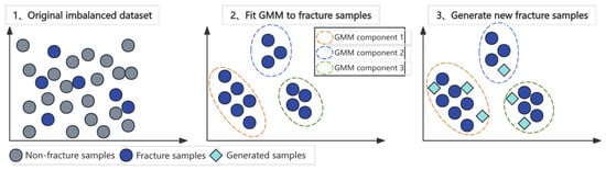
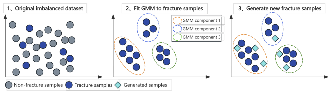
Fracture prediction based on well-log data is characterized by a severe class imbalance because fracture-bearing intervals generally account for only a small proportion of the entire logged interval. In the dataset used in this study, fracture samples accounted for 0.60% and 1.34% of the original samples in WELL1 and WELL2, respectively. Therefore, a hybrid balancing strategy combining depth-uniform undersampling and Gaussian mixture model (GMM)-based fracture-sample augmentation was applied to the training set. The former reduces redundant non-fracture samples while maintaining their coverage along the depth direction, whereas the latter learns the distribution of fracture responses and generates diverse synthetic fracture samples. As illustrated in Figure 1, the GMM-based augmentation first models the distribution of fracture samples and then generates new samples from the learned distribution.

Figure 1. Schematic of GMM-based fracture sample augmentation.

Let the non-fracture and fracture samples in the original training set be denoted by

$${\mathcal{D}}_{-}={\left\{({\mathbf{x}}_i^{-},0)\right\}}_{i=1}^{N_{-}},$$

(1)

and

$${\mathcal{D}}_{+}={\left\{({\mathbf{x}}_i^{+},1)\right\}}_{i=1}^{N_{+}},$$

(2)

where ${\mathbf{x}}_i^{-},{\mathbf{x}}_i^{+}\in {\mathbb{R}}^C$ represent the multivariate features of the i-th non-fracture and fracture samples, respectively. $N_{-}$ and $N_{+}$ are the numbers of non-fracture and fracture samples, respectively. Generally, $N_{-}\gg N_{+}$.

Because well-log measurements at adjacent depths are strongly correlated, a large number of neighboring non-fracture samples may contain highly redundant information. During the undersampling process, the samples in ${\mathcal{D}}_{-}$ were first ordered according to their logging depths and then selected at uniform depth intervals. The resulting subset is denoted by ${\mathcal{D}}_{-}^{\mathrm{sub}}$. This procedure reduces the dominance of the majority class while retaining representative non-fracture samples over the entire target interval. All real fracture samples were retained during this process.

The statistical distribution of fracture-related logging responses is generally multimodal because it can be affected by lithology, fracture type, fracture filling, and other geological conditions. A single Gaussian distribution is therefore insufficient to describe the heterogeneous distribution of the fracture samples. In this study, a GMM with K Gaussian components was employed to approximate the joint probability distribution of the real fracture samples:

$$p(\mathbf{x}\mid \mathsf{\Theta })={\displaystyle \sum _{k=1}^K}{\pi }_k\mathcal{N}\left(\mathbf{x}\mid {\mathit{\mu }}_k,{\mathsf{\Sigma }}_k\right),$$

(3)

where ${\pi }_k$, ${\mathit{\mu }}_k$, and ${\mathbf{\Sigma }}_k$ denote the mixing coefficient, mean vector, and covariance matrix of the k-th Gaussian component, respectively. The mixing coefficients satisfy

$${\pi }_k\ge 0,{\displaystyle \sum _{k=1}^K}{\pi }_k=1.$$

(4)

Each Gaussian component represents a local response pattern of fracture-bearing intervals in the multivariate feature space, whereas the weighted combination of all components describes the overall distribution of the fracture class. The number of Gaussian components was determined using the Bayesian information criterion (BIC), which balances the goodness of fit against model complexity. For a candidate component number K, the BIC is defined as

$$\mathrm{BIC}\left(K\right)=-2\ln {\widehat{\mathcal{L}}}_K+q_K\ln N_{+},$$

(5)

where ${\widehat{\mathcal{L}}}_K$ is the maximized likelihood of the GMM with K components, and $q_K$ is the corresponding number of free model parameters. The optimal number of components was selected as

$$K^{*}=\arg \underset{K}{\min }\mathrm{BIC}\left(K\right).$$

(6)

After $K^{*}$ was determined, the GMM parameters $\mathsf{\Theta }={\{{\pi }_k,{\mathit{\mu }}_k,{\mathsf{\Sigma }}_k\}}_{k=1}^{K^{*}}$ were estimated from the real fracture samples using the expectation–maximization algorithm.

Synthetic fracture samples were subsequently generated from the fitted GMM. For each synthetic sample, a Gaussian component was first selected according to its mixing coefficient:

$$k\sim Categorical({\pi }_1,{\pi }_2,\dots ,{\pi }_{K^{*}}).$$

(7)

A new sample was then drawn from the selected component:

$${\mathbf{x}}^{\mathrm{syn}}\sim \mathcal{N}\left({\mathit{\mu }}_k,{\mathsf{\Sigma }}_k\right).$$

(8)

The sampling procedure was repeated until the number of generated fracture samples reached r (augmentation factor) times the number of original fracture samples. The resulting synthetic fracture samples were then combined with the retained non-fracture samples and the original fracture samples to construct the augmented training set. Let the generated fracture sample set be

$${\mathcal{D}}_{+}^{\mathrm{syn}}={\left\{({\mathbf{x}}_i^{\mathrm{syn}},1)\right\}}_{i=1}^{N_{\mathrm{syn}}}.$$

(9)

The augmented training set was finally constructed as

$${\mathcal{D}}_{\mathrm{train}}^{\mathrm{aug}}={\mathcal{D}}_{-}^{\mathrm{sub}}\cup {\mathcal{D}}_{+}\cup {\mathcal{D}}_{+}^{\mathrm{syn}}.$$

(10)

2.2. iTransformer-LSTM Network

The logging responses associated with fractures are characterized by two types of dependencies. At each depth position, different logging variables respond to fractures from different physical perspectives and therefore present complex and sample-dependent inter-feature relationships. Meanwhile, fracture-related anomalies often vary continuously within local depth intervals, introducing depth-dependent contextual information. Based on these characteristics, the iTransformer and LSTM are assigned distinct modeling roles rather than being simply stacked. Specifically, the iTransformer treats the selected logging variables as feature tokens and learns adaptive inter-feature dependencies at each depth position. The resulting representations within a local physical-depth window are then arranged according to depth and processed by the LSTM to capture sequential variations along the depth direction. In this way, the proposed network explicitly separates feature-space interaction modeling from depth-space contextual modeling.

For the i-th sample, the selected logging features are represented as

$${\mathbf{x}}_i=[x_{i,1},x_{i,2},\dots ,x_{i,C}]\in {\mathbb{R}}^C,$$

(11)

where C denotes the number of selected input features and $x_{i,c}$ represents the value of the c-th logging feature for the ith sample. In this study, six features were retained as the inputs of the iTransformer-LSTM network.

2.2.1. iTransformer

To explicitly model the dependencies among different logging features, each selected feature is treated as an individual token. Unlike conventional Transformer architectures in which tokens usually correspond to sequential observations, the self-attention mechanism here operates along the feature dimension, allowing the network to directly learn interactions among different features [23].

Each scalar feature $x_{i,c}$ is first projected into a $d_{\mathrm{model}}$-dimensional latent representation through a learnable linear mapping:

$${\mathbf{e}}_{i,c}=x_{i,c}{\mathbf{w}}_e+{\mathbf{b}}_e+{\mathbf{p}}_c,c=1,\dots ,C,$$

(12)

where ${\mathbf{w}}_e\in {\mathbb{R}}^{d_{\mathrm{model}}}$ and ${\mathbf{b}}_e\in {\mathbb{R}}^{d_{\mathrm{model}}}$ denote the learnable projection parameters, and ${\mathbf{p}}_c\in {\mathbb{R}}^{d_{\mathrm{model}}}$ is a learnable embedding associated with the c-th feature. The embedded feature representations are then stacked as

$${\mathbf{H}}_i^{\left(0\right)}=[{\mathbf{e}}_{i,1};{\mathbf{e}}_{i,2};\dots ;{\mathbf{e}}_{i,C}]\in {\mathbb{R}}^{C\times d_{\mathrm{model}}},$$

(13)

where each row corresponds to one feature token.

For the h-th attention head, the query, key, and value matrices are obtained from the input representation as

$${\mathbf{Q}}_h={\mathbf{H}}_i^{(l-1)}{\mathbf{W}}_h^Q,{\mathbf{K}}_h={\mathbf{H}}_i^{(l-1)}{\mathbf{W}}_h^K,{\mathbf{V}}_h={\mathbf{H}}_i^{(l-1)}{\mathbf{W}}_h^V,$$

(14)

where ${\mathbf{H}}_i^{(l-1)}$ denotes the input representation of the l-th attention layer, and ${\mathbf{W}}_h^Q$, ${\mathbf{W}}_h^K$, and ${\mathbf{W}}_h^V$ are the learnable projection matrices for the query, key, and value of the h-th attention head, respectively. The scaled dot-product attention for the h-th head is calculated as

$${head}_h=softmax\left({\displaystyle \frac{{\mathbf{Q}}_h{\mathbf{K}}_h^{\mathrm{T}}}{\sqrt{d_k}}}\right){\mathbf{V}}_h,$$

(15)

where $d_k$ denotes the dimension of the key vectors.

The outputs of all attention heads are concatenated and projected back to the model dimension:

$$MHA\left({\mathbf{H}}_i^{(l-1)}\right)=Concat\left({head}_1,\dots ,{head}_H\right){\mathbf{W}}^O,$$

(16)

where H denotes the number of attention heads and ${\mathbf{W}}^O$ is the output projection matrix.

Since the attention operation is performed among the C feature tokens, the attention weight matrix has a dimension of $C\times C$. Each element characterizes the learned dependency between two logging features, enabling the network to identify their joint response patterns associated with fracture development.

In the proposed network, two multi-head self-attention layers are applied successively:

$${\mathbf{H}}_i^{\left(1\right)}=LayerNorm\left({\mathbf{H}}_i^{\left(0\right)}+Dropout\left[{MHA}_1\left({\mathbf{H}}_i^{\left(0\right)}\right)\right]\right),$$

(17)

and

$${\mathbf{H}}_i^{\left(2\right)}=LayerNorm\left({\mathbf{H}}_i^{\left(1\right)}+Dropout\left[{MHA}_2\left({\mathbf{H}}_i^{\left(1\right)}\right)\right]\right).$$

(18)

The resulting representation ${\mathbf{H}}_i^{\left(2\right)}\in {\mathbb{R}}^{C\times d_{\mathrm{model}}}$ contains attention-enhanced representations of the selected logging features.

2.2.2. LSTM

After the dependencies among different logging features are modeled by the iTransformer, an LSTM is further employed to characterize the local variation of logging responses along the depth direction. For each target depth $d_i$, a local physical-depth window containing L uniformly resampled depth positions is constructed around it. The window is defined with a physical radius R, covering the depth interval from $d_i-R$ to $d_i+R$. The effect of the physical window radius R is further investigated in Section 3.5. Let

$$m={\displaystyle \frac{L-1}{2}},$$

(19)

where m denotes the number of depth positions considered on each side of the target depth. The local window therefore contains L ordered depth positions centered at $d_i$, covering the logging responses above and below the target depth.

The feature self-attention operation described above is applied independently at each depth position within the local window. Accordingly, for the k-th depth position in the local window, the output of the iTransformer is

$${\mathbf{H}}_k^{\left(2\right)}\in {\mathbb{R}}^{C\times d_{\mathrm{model}}},$$

(20)

where ${\mathbf{H}}_k^{\left(2\right)}$ contains the attention-enhanced representations of the C selected logging features at that depth position.

To obtain a compact representation of each depth position, mean pooling is performed along the feature dimension. Let ${\mathbf{H}}_{k,c}^{\left(2\right)}\in {\mathbb{R}}^{d_{\mathrm{model}}}$ denote the representation of the c-th logging feature. The aggregated representation at the k-th depth position is calculated as

$${\mathbf{r}}_k={\displaystyle \frac{1}{C}}{\displaystyle \sum _{c=1}^C}{\mathbf{H}}_{k,c}^{\left(2\right)},{\mathbf{r}}_k\in {\mathbb{R}}^{d_{\mathrm{model}}}.$$

(21)

In this manner, the attention-enhanced representations of all selected logging features are summarized into a single latent representation while retaining the cross-feature dependencies learned by the preceding self-attention layers.

For the target depth $d_i$, the pooled representations within the local physical-depth window are arranged according to their depth order as

$${\mathbf{R}}_i=\left[{\mathbf{r}}_1,{\mathbf{r}}_2,\dots ,{\mathbf{r}}_{m+1},\dots ,{\mathbf{r}}_L\right]\in {\mathbb{R}}^{L\times d_{\mathrm{model}}},$$

(22)

where ${\mathbf{r}}_{m+1}$ corresponds to the target depth $d_i$, while the preceding and succeeding representations correspond to the resampled positions above and below $d_i$, respectively. Thus, ${\mathbf{R}}_i$ preserves the physical depth order of the local logging responses.

The sequence ${\mathbf{R}}_i$ is subsequently processed by the LSTM from shallower to deeper positions within the local window. At each depth position, the current representation is combined with the information propagated from the preceding depth positions. This process can be expressed as

$${\mathbf{s}}_k=LSTM\left({\mathbf{r}}_k,{\mathbf{s}}_{k-1}\right),k=1,\dots ,L,$$

(23)

where ${\mathbf{s}}_k$ denotes the sequential representation at the k-th depth position. For the first position in each local window, the recurrent state is initialized to zero. Through this recurrent process, logging information is progressively propagated from shallower to deeper positions, enabling the network to characterize the local depth-dependent variation of fracture-related logging responses.

After all L depth positions have been processed, the final sequential representation

$${\mathbf{s}}_L\in {\mathbb{R}}^{d_{\mathrm{hidden}}}$$

(24)

is used as the integrated representation of the local logging interval centered at $d_i$. It is subsequently passed to the fully connected classification layer to obtain the fracture prediction for the target depth.

2.2.3. iTransformer-LSTM Integration

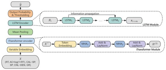
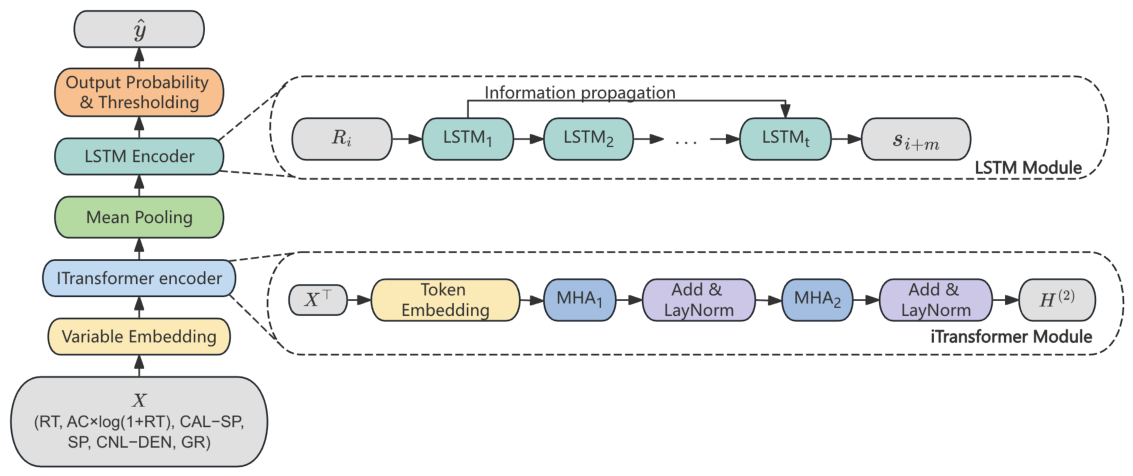
The proposed network integrates the iTransformer and LSTM in a serial manner to jointly model inter-feature dependencies and local depth-dependent variations (as shown in Figure 2).

Figure 2. Schematic of the proposed iTransformer-LSTM network architecture. Arrows indicate the direction of data flow, colors distinguish functional components, and dashed boxes show the internal structures of the corresponding modules.

For each depth position $d_k$ within the local window centered at $d_i$, the iTransformer first models the nonlinear dependencies among the C selected logging features and generates the attention-enhanced representation

$${\mathbf{H}}_k^{\left(2\right)}=f_{\mathrm{iTransformer}}\left({\mathbf{x}}_k\right)\in {\mathbb{R}}^{C\times d_{\mathrm{model}}}.$$

(25)

The C feature representations are subsequently aggregated through mean pooling along the feature dimension to obtain a unified representation $\mathbf{r}k\in {\mathbb{R}}^{d\mathrm{model}}$ for each depth position. The resulting representations within the local window are arranged according to their physical depth order:

$${\mathbf{R}}_i=\left[{\mathbf{r}}_{i-m},\dots ,{\mathbf{r}}_i,\dots ,{\mathbf{r}}_{i+m}\right]\in {\mathbb{R}}^{L\times d_{\mathrm{model}}}.$$

(26)

The LSTM then processes ${\mathbf{R}}_i$ along the depth direction and produces the final sequential representation

$${\mathbf{s}}_{i+m}=f_{\mathrm{LSTM}}\left({\mathbf{R}}_i\right),$$

(27)

where ${\mathbf{s}}_{i+m}$ integrates the local depth-dependent logging information within the physical-depth window centered at $d_i$.

The final sequential representation is passed through a fully connected classification layer to obtain the class scores:

$${\mathbf{o}}_i={\mathbf{W}}_c{\mathbf{s}}_{i+m}+{\mathbf{b}}_c,$$

(28)

where ${\mathbf{W}}_c$ and ${\mathbf{b}}_c$ are the learnable parameters of the classification layer. The predicted class-probability vector is then obtained using the softmax function:

$${\widehat{\mathbf{p}}}_i=softmax\left({\mathbf{o}}_i\right),$$

(29)

where ${\widehat{p}}_i$ represents the predicted probability of fracture occurrence at the target depth $d_i$. A sample is classified as a fracture when its predicted fracture probability is greater than or equal to a decision threshold $\theta$.

3. Results

3.1. Experimental Dataset and Data Preprocessing

All experiments were implemented in Python 3.8.10 using PyTorch 2.3.1 with CUDA 12.1. Neural-network training was performed on an NVIDIA RTX A6000 GPU. The experimental dataset was collected from the C7 target interval of two wells in the study area. C7 refers to the Chang 7 oil-bearing member of the Yanchang Formation in the Ordos Basin. The available conventional well logs included acoustic transit time (AC), bulk density (DEN), compensated neutron log (CNL), gamma ray (GR), deep resistivity (RT), spontaneous potential (SP), and caliper (CAL). Fracture labels were determined from core observations and formation microimager (FMI) interpretations, with fracture and non-fracture samples labeled as 1 and 0, respectively. Table 1 and Table 2 summarize the well information and logging statistics, respectively.

Table 1. Basic information of the experimental well-log dataset.

Well	Depth Start (m)	Depth End (m)	Samples	Fracture Samples	Fracture Ratio (%)
WELL1	1800.00	1909.99	11,000	66	0.60
WELL2	2330.09	2442.03	1122	15	1.34

Table 2. Statistical characteristics of the conventional logging variables.

Logging Variable	Unit	WELL1	WELL2
AC	μs/m	237.60 ± 31.37	255.81 ± 29.61
DEN	g/cm3	2.53 ± 0.13	2.53 ± 0.12
CNL	%	20.84 ± 8.91	27.84 ± 9.11
GR	API	166.30 ± 120.41	175.60 ± 80.48
RT	Ω·m	52.16 ± 38.01	156.47 ± 97.48
SP	mV	54.41 ± 17.92	176.29 ± 304.05
CAL	cm	22.88 ± 0.68	22.08 ± 0.59

Note: Values are reported as mean ± standard deviation.

The original WELL1 dataset exhibited a severe class imbalance, with fracture samples accounting for only 0.60% of the samples. To alleviate the dominance of non-fracture samples during model training while maintaining representative coverage over the investigated depth interval, a depth-based uniform undersampling strategy was applied to WELL1. All fracture samples were retained, whereas non-fracture samples were uniformly selected along the depth direction rather than randomly discarded. After undersampling, WELL1 contained 134 samples, including 66 fracture samples and 68 non-fracture samples, increasing the fracture proportion to 49.25%.

WELL2 was treated as an independent blind well for cross-well evaluation and was therefore not subjected to undersampling. All valid samples from the complete WELL2 interval were retained for testing, so that the evaluation reflected the original class distribution and the practical difficulty of fracture identification under severe class imbalance. In WELL2, fracture samples accounted for only 1.34% of the original data.

Because fracture development is generally characterized by coordinated anomalies in multiple logging curves rather than the independent response of a single variable, several composite logging features were further constructed. These features included the ratios $AC/DEN$ and $RT/GR$, the differences $CNL-DEN$ and $CAL-SP$, and the nonlinear coupling term $AC\times \log (1+RT)$. These engineered features were introduced as expert-informed low-order representations of interactions among acoustic, density, neutron, resistivity, gamma-ray, spontaneous-potential, and caliper responses. They were not used as substitutes for the adaptive inter-feature modeling of the iTransformer.

The samples from WELL1 were randomly divided into training, validation, and test subsets at a ratio of 8:1:1, while WELL2 was used as the prediction set. The training subset was used for model parameter optimization, the validation subset was used for model selection and decision-threshold $\theta$ determination, and the test subset was used to evaluate the trained model on held-out samples from WELL1.

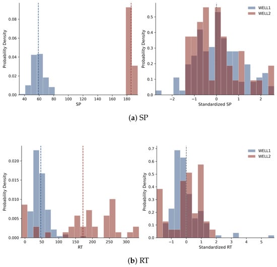
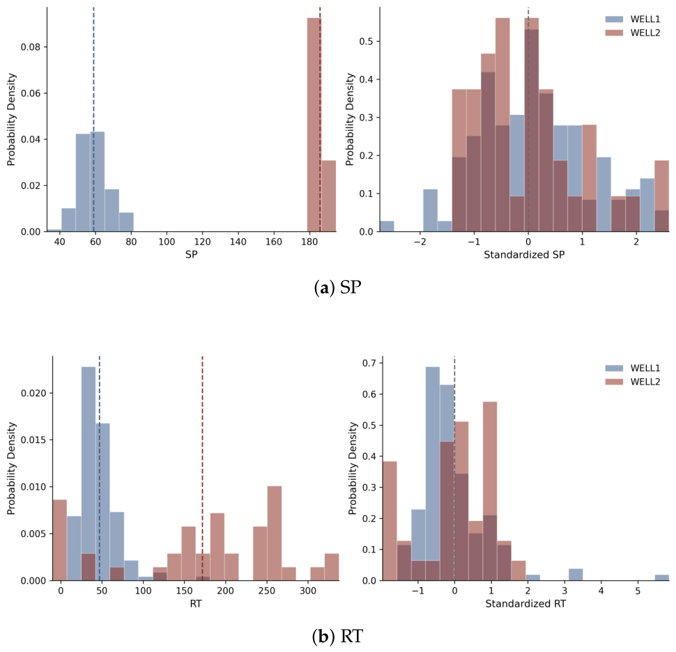
As shown in Table 2, noticeable differences exist in the numerical scales and statistical distributions of the logging variables between WELL1 and WELL2, particularly for RT and SP. To reduce the influence of these differences on subsequent feature processing and model training, a well-specific Z-score standardization strategy was adopted. Specifically, for WELL1, the mean ${\mu }_i$ and standard deviation ${\sigma }_i$ of the i-th logging feature were calculated using only the training subset. The same statistics were then applied to standardize the training, validation, and test subsets of WELL1. For WELL2, Z-score standardization was performed independently for each logging feature:

$$x_i^{\prime }={\displaystyle \frac{x_i-{\mu }_i}{{\sigma }_i}},$$

(30)

where $x_i$ and $x_i^{\prime }$ are the original and standardized feature values, and ${\mu }_i$ and ${\sigma }_i$ are the corresponding mean and standard deviation. Figure 3 shows the SP and RT distributions before and after standardization.

Figure 3. Distributions of SP and RT in WELL1 and WELL2 before and after Z-score standardization. (a) SP distribution. (b) RT distribution. The dashed vertical lines indicate the mean values of the corresponding distributions.

3.2. Feature Selection Based on Random Forest Importance and Mutual Information

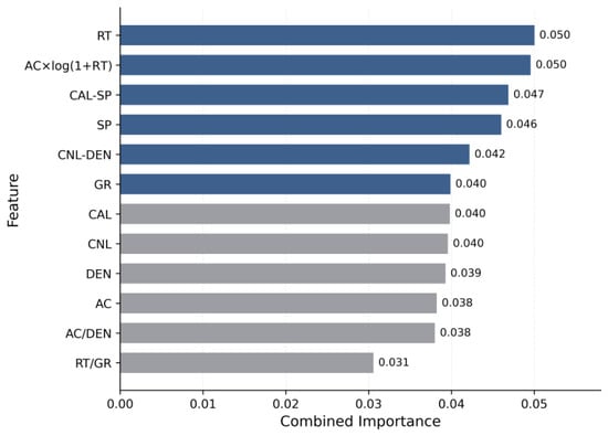
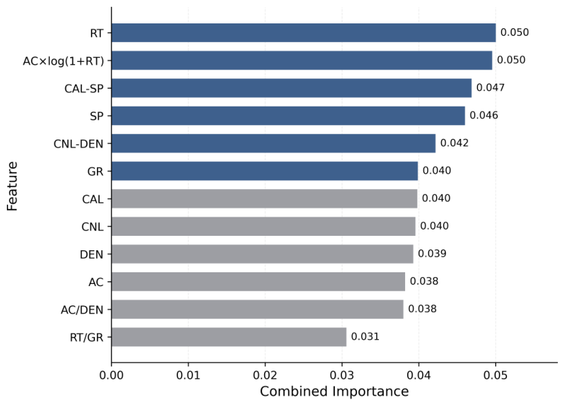
To reduce feature redundancy and retain the logging variables most informative for fracture identification, random forest feature importance and mutual information were jointly employed to rank the candidate features. Random forest importance evaluates feature relevance from a model-based perspective by measuring its contribution to class discrimination, whereas mutual information evaluates feature relevance from a statistical perspective by quantifying its dependence on the fracture label.

For the random forest, multiple decision trees were constructed from the training data. At each split, the feature that produced the greatest reduction in node impurity was preferentially selected. Features that were repeatedly used for effective splitting across the ensemble and contributed more strongly to distinguishing fracture and non-fracture samples consequently received higher importance scores. The importance of the j-th feature can be expressed as the accumulated impurity reduction associated with that feature over all trees:

$$I_j^{\mathrm{RF}}={\displaystyle \frac{1}{T}}{\displaystyle \sum _{t=1}^T}\sum _{n\in \mathcal{N}j,t}\Delta \mathcal{I}n,t,$$

(31)

where T is the number of trees, ${\mathcal{N}}_{j,t}$ denotes the set of nodes in the tth tree split using the j-th feature, and $\Delta {\mathcal{I}}_{n,t}$ is the impurity reduction produced at node n.

Mutual information was further used to characterize nonlinear statistical dependence between each candidate feature and the fracture label. For a feature $X_j$ and class label Y, the mutual information is defined as

$$I(X_j;Y)=\sum _{x_j}\sum _{y}p(x_j,y)\log {\displaystyle \frac{p(x_j,y)}{p\left(x_j\right)p\left(y\right)}},$$

(32)

where $p(x_j,y)$ denotes the joint probability distribution of $X_j$ and Y, while $p\left(x_j\right)$ and $p\left(y\right)$ are their marginal distributions. A larger mutual information value indicates that the corresponding logging feature contains more information relevant to fracture discrimination.

Because the numerical ranges of the random forest importance and mutual information scores are different, both scores were normalized before fusion. The normalized scores were calculated as

$${\tilde{I}}_j^{\mathrm{RF}}={\displaystyle \frac{I_j^{\mathrm{RF}}}{{\sum }_{k=1}^M{I}_k^{\mathrm{RF}}}},{\tilde{I}}_j^{\mathrm{MI}}={\displaystyle \frac{I_j^{\mathrm{MI}}}{{\sum }_{k=1}^M{I}_k^{\mathrm{MI}}}},$$

(33)

where M is the total number of candidate features. The final feature score was then obtained using equal weighting:

$$S_j=0.5\tilde{I}{j}^{\mathrm{RF}}+0.5\tilde{I}{j}^{\mathrm{MI}}.$$

(34)

The normalized random forest importance and mutual information scores were assigned equal weights to obtain the combined feature importance score $S_j$. As shown in Figure 4, all candidate features were ranked in descending order according to $S_j$, and the six highest-ranked features, namely $RT$, $AC\times \log (1+RT)$, $CAL-SP$, $SP$, $CNL-DEN$, and $GR$, were retained as the model inputs.

Figure 4. Ranking of candidate features based on the combined random forest importance and mutual information score.

3.3. Fracture Classification Results

To evaluate the fracture classification performance, several representative supervised learning methods were employed for comparison, including Random Forest (RF), support vector machine (SVM), multilayer perceptron (MLP), XGBoost, and LightGBM, as well as two recent neural-network-based approaches adapted from FIsr [19] and UGIN [20]. These methods represent different learning mechanisms: RF performs classification through an ensemble of decision trees, SVM constructs a nonlinear decision boundary in the feature space, MLP learns nonlinear mappings through fully connected neural layers, while XGBoost and LightGBM employ gradient-boosted decision trees to progressively improve classification performance. In addition, FIsr employs a sliding-window sequence representation combined with recurrent neural-network modeling to capture local depth-dependent variations, whereas UGIN introduces graph-based representation learning to model relationships among well-log samples. All baseline models were evaluated under the same data preprocessing, data split, and five-run protocol as the proposed iTransformer-LSTM model to ensure a consistent comparison.

For all methods, WELL1 was divided into training, validation, and test sets at a ratio of 8:1:1. Fracture samples in the training set were augmented using a Gaussian mixture model (GMM) with an augmentation factor of 0.1, indicating that the number of synthetic fracture samples generated by GMM was set to $10\%$ of the original fracture samples in the training set. The BIC analysis selected $K=3$, which was used in all subsequent experiments. A full covariance matrix with a regularization term of $1\times {10}^{-6}$ was adopted. This choice accommodates coordinated variations in fracture-related logging responses. For the proposed iTransformer-LSTM, the local physical-depth window length was set to $L=5$, corresponding to two depth positions on each side of the target depth ($m=2$). The embedding dimension of the iTransformer was set to $d_{\mathrm{model}}=16$, with one attention head and two successive multi-head self-attention layers. The LSTM consisted of a single recurrent layer with a hidden dimension of 16. The Adam optimizer was employed with an initial learning rate of 0.001 and a weight-decay coefficient of 0.0001. The maximum number of training epochs was set to 100, with a mini-batch size of 16. A dropout rate of 0.1 was applied after the multi-head attention layers to reduce overfitting. Early stopping was adopted based on the validation loss, and training was terminated if the validation loss did not improve for 20 consecutive epochs.

Early stopping was also applied to XGBoost and LightGBM during their iterative training. For each model, the classification threshold was independently selected on the validation set by searching from 0.1 to 0.9 with a step size of 0.01 and maximizing the macro-F1 score. The selected threshold was subsequently fixed for evaluation on the WELL1 test set and WELL2.

To provide a more reliable comparison among the proposed method and the baseline models and to reduce the influence of randomness in model training, all models were evaluated over five runs with different random seeds. The experimental results are reported as the mean and standard deviation across the five runs.

The comparative results on the WELL1 test set are summarized in Table 3. The iTransformer-LSTM achieved the best overall performance, with an accuracy of $0.714\pm 0.038$, a macro-F1 score of $0.708\pm 0.093$, and an AUC of $0.816\pm 0.042$. It outperformed both the conventional machine learning baselines and the adapted recent neural-network-based approaches, with particularly clear improvements in macro-F1 and AUC. These results indicate that the proposed model provides a better balance between fracture and non-fracture identification while maintaining stronger discriminative capability on WELL1.

Table 3. Classification results of different models on the WELL1 test set.

Model	Accuracy	Macro-F1	AUC
Random Forest	$0.617\pm 0.046$	$0.613\pm 0.045$	$0.606\pm 0.024$
SVM	$0.533\pm 0.112$	$0.345\pm 0.053$	$0.454\pm 0.006$
MLP	$0.583\pm 0.059$	$0.535\pm 0.115$	$0.623\pm 0.089$
XGBoost	$0.583\pm 0.059$	$0.564\pm 0.082$	$0.631\pm 0.023$
LightGBM	$0.600\pm 0.037$	$0.596\pm 0.034$	$0.571\pm 0.040$
FIsr [19]	$0.543\pm 0.108$	$0.499\pm 0.146$	$0.539\pm 0.101$
UGIN [20]	$0.500\pm 0.087$	$0.468\pm 0.095$	$0.584\pm 0.145$
iTransformer-LSTM	$\mathbf{0.714}\pm \mathbf{0.038}$	$\mathbf{0.708}\pm \mathbf{0.093}$	$\mathbf{0.816}\pm \mathbf{0.042}$

Note: Bold numerical values indicate the highest mean performance for each metric within each well.

As shown in Table 4, iTransformer-LSTM achieved the highest Macro-F1 score, AUC, and fracture recall on WELL2. Although LightGBM obtained the highest accuracy, its substantially lower fracture recall indicates a strong bias toward the majority non-fracture class. By contrast, iTransformer-LSTM demonstrated a better balance between overall discrimination and fracture detection, which is particularly important under the highly imbalanced class distribution of WELL2.

Table 4. Fracture classification results of different models on WELL2 over five independent runs.

Model	Accuracy	Macro-F1	AUC	Fracture Recall	Mean Confusion Matrix
Random Forest	$0.487\pm 0.018$	$0.345\pm 0.008$	$0.659\pm 0.014$	$0.787\pm 0.056$	$\left[\begin{array}{cc}533.8& 571.2\\ 3.2& 11.8\end{array}\right]$
SVM	$0.354\pm 0.048$	$0.266\pm 0.028$	$0.295\pm 0.002$	$0.347\pm 0.030$	$\left[\begin{array}{cc}391.8& 713.2\\ 9.8& 5.2\end{array}\right]$
MLP	$0.629\pm 0.362$	$0.356\pm 0.194$	$0.392\pm 0.073$	$0.293\pm 0.407$	$\left[\begin{array}{cc}699.6& 405.4\\ 10.6& 4.4\end{array}\right]$
XGBoost	$0.724\pm 0.169$	$0.441\pm 0.068$	$0.698\pm 0.019$	$0.520\pm 0.185$	$\left[\begin{array}{cc}803.0& 302.0\\ 7.2& 7.8\end{array}\right]$
LightGBM	$\mathbf{0.941}\pm \mathbf{0.011}$	$0.496\pm 0.003$	$0.658\pm 0.012$	$0.053\pm 0.030$	$\left[\begin{array}{cc}1052.8& 52.2\\ 14.2& 0.8\end{array}\right]$
FIsr [19]	$0.791\pm 0.063$	$0.473\pm 0.022$	$0.725\pm 0.025$	$0.520\pm 0.128$	$\left[\begin{array}{cc}878.6& 226.4\\ 7.2& 7.8\end{array}\right]$
UGIN [20]	$0.808\pm 0.085$	$0.469\pm 0.027$	$0.692\pm 0.054$	$0.347\pm 0.173$	$\left[\begin{array}{cc}900.2& 204.8\\ 9.8& 5.2\end{array}\right]$
iTransformer-LSTM	$0.816\pm 0.093$	$\mathbf{0.502}\pm \mathbf{0.034}$	$\mathbf{0.734}\pm \mathbf{0.016}$	$\mathbf{0.813}\pm \mathbf{0.163}$	$\left[\begin{array}{cc}902.6& 202.4\\ 2.8& 12.2\end{array}\right]$

Note: The mean confusion matrices are reported in the order $\left[\begin{array}{cc}\mathrm{TN}& \mathrm{FP}\\ \mathrm{FN}& \mathrm{TP}\end{array}\right]$, where TN, FP, FN, and TP denote true negatives, false positives, false negatives, and true positives, respectively. Bold numerical values indicate the highest mean performance for each metric within each well.

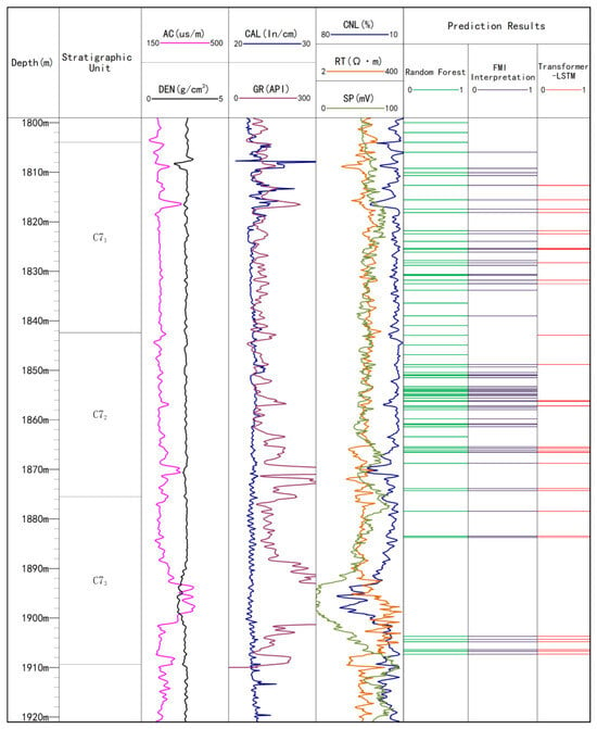
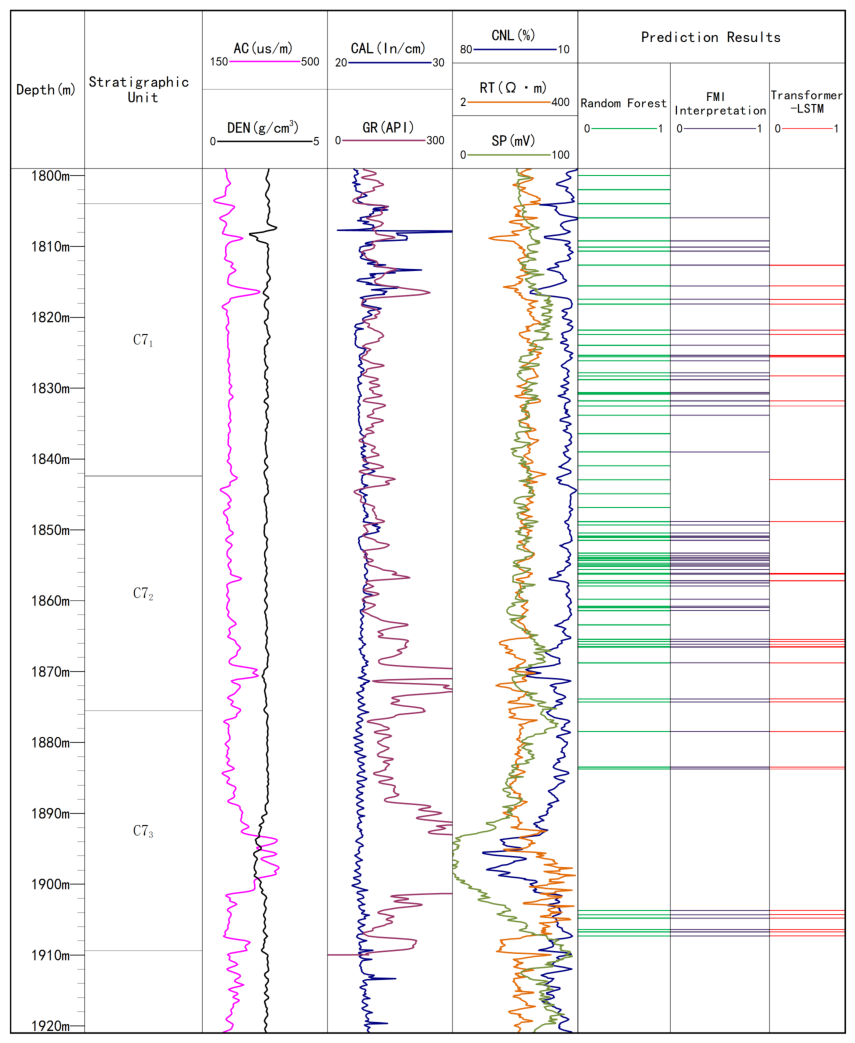
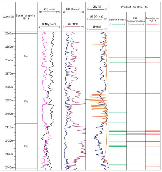
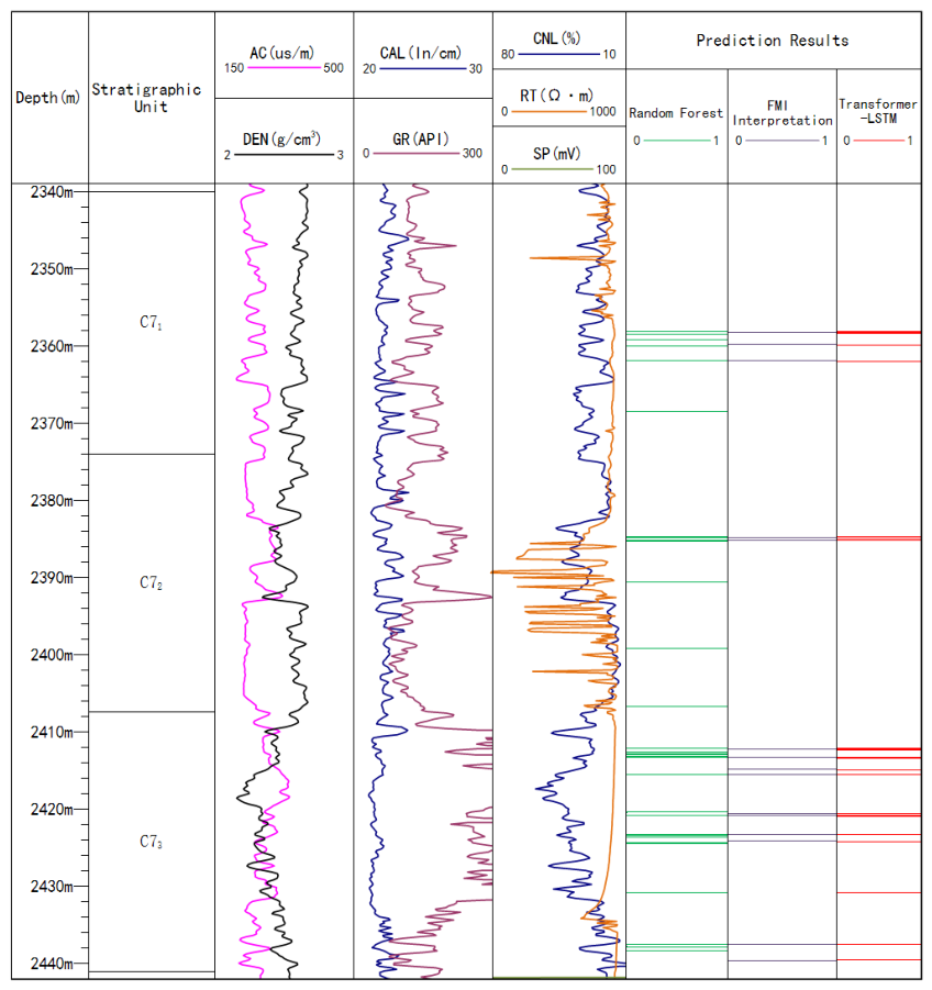
In addition to the quantitative evaluation, comprehensive well-log plots were constructed to provide a more intuitive visualization of the fracture prediction results. As shown in Figure 5 and Figure 6, the conventional logging curves, stratigraphic units, FMI-interpreted fractures, and fracture prediction results are displayed along the depth axis for WELL1 and WELL2, respectively.

Figure 5. Comparison of fracture prediction results with FMI interpretation for WELL1.

Figure 6. Comparison of fracture prediction results with FMI interpretation for WELL2.

3.4. Ablation Study on GMM-Based Data Augmentation

To investigate the effect of GMM-based fracture-sample augmentation, an ablation study was conducted on the iTransformer-LSTM model. The augmentation factor r was set to 0, 0.1, 0.2, 0.3, 0.4 and 0.5, representing the ratio of generated fracture samples to the original fracture samples, with $r=0$ denoting no GMM augmentation.

As shown in Table 5, the augmentation factor affects the performance of the iTransformer-LSTM model. On WELL1, $r=0.1$ achieved noticeably better average results than $r=0$. However, because the WELL1 test set is small, the corresponding metrics are relatively sensitive to the prediction of a limited number of samples. To reduce the influence of random variation, each augmentation setting was evaluated over five independent runs and reported as mean ± standard deviation. On the independent WELL2 blind-well test, where the complete well data and the original imbalanced class distribution were retained, the improvement introduced by $r=0.1$ was more moderate. This result suggests that GMM augmentation can provide additional variations of fracture-related logging responses when real fracture samples are limited, thereby reducing the model’s dependence on the small number of observed fracture samples and improving its generalization capability.

Table 5. Effect of the GMM augmentation factor on the performance of the iTransformer-LSTM model.

Factor r	WELL1			WELL2
	Accuracy	Macro-F1	AUC	Accuracy	Macro-F1	AUC
0.0	$0.543\pm 0.108$	$0.498\pm 0.141$	$0.510\pm 0.145$	$0.812\pm 0.093$	$0.479\pm 0.034$	$0.734\pm 0.016$
0.1	$\mathbf{0.714}\pm \mathbf{0.038}$	$\mathbf{0.708}\pm \mathbf{0.093}$	$\mathbf{0.816}\pm \mathbf{0.042}$	$\mathbf{0.816}\pm \mathbf{0.093}$	$\mathbf{0.502}\pm \mathbf{0.034}$	$\mathbf{0.734}\pm \mathbf{0.016}$
0.2	$0.500\pm 0.051$	$0.455\pm 0.088$	$0.588\pm 0.147$	$0.558\pm 0.161$	$0.372\pm 0.072$	$0.666\pm 0.112$
0.3	$0.486\pm 0.060$	$0.462\pm 0.070$	$0.608\pm 0.117$	$0.669\pm 0.208$	$0.416\pm 0.085$	$0.693\pm 0.064$
0.4	$0.529\pm 0.148$	$0.485\pm 0.178$	$0.555\pm 0.100$	$0.533\pm 0.120$	$0.363\pm 0.057$	$0.655\pm 0.088$
0.5	$0.514\pm 0.117$	$0.439\pm 0.164$	$0.551\pm 0.151$	$0.517\pm 0.178$	$0.353\pm 0.089$	$0.645\pm 0.135$

Note: Bold numerical values indicate the highest mean performance for each metric within each well.

When the augmentation factor was further increased, the performance generally deteriorated on both wells. This suggests that the role of GMM-based augmentation is not to substantially enlarge the training set, but rather to introduce a limited amount of distributional variation into the minority fracture class. A moderate augmentation ratio may help reduce the model’s dependence on the specific fracture-response patterns observed in WELL1, whereas excessive synthetic sampling may progressively distort the original minority-class distribution and adversely affect model performance. Therefore, $r=0.1$ was selected as the augmentation factor in the subsequent experiments.

3.5. Effect of Physical Window Radius

The LSTM module models the sequential variation of logging responses along the depth direction. Therefore, the physical depth range covered by its input sequence determines the extent of local depth context available for fracture identification. To investigate the influence of this context range, experiments were conducted using different physical window radius R. For a target depth $d_i$, the local window covers the interval $[d_i-R,d_i+R]$. The number of resampled depth positions was fixed at $L=5$, while R was varied from 0.05 to 0.30 m. All other experimental settings were kept unchanged to ensure a fair comparison.

As shown in Table 6, the physical window radius has a noticeable influence on the prediction performance of the iTransformer-LSTM model. On WELL1, $R=0.10$ m achieved the best performance across all three evaluation metrics, indicating that a compact local depth range is sufficient to capture the fracture-related contextual information within the training well. On the independent WELL2 blind-well test, $R=0.10$ m also achieved the highest accuracy and Macro-F1, whereas a slightly larger radius of $R=0.20$ m produced the highest AUC.

Table 6. Effect of the physical window radius on the performance of the iTransformer-LSTM model.

R (m)	WELL1			WELL2
	Accuracy	Macro-F1	AUC	Accuracy	Macro-F1	AUC
0.05	$0.600\pm 0.130$	$0.594\pm 0.131$	$0.706\pm 0.067$	$0.685\pm 0.094$	$0.434\pm 0.038$	$0.749\pm 0.011$
0.10	$\mathbf{0.714}\pm \mathbf{0.038}$	$\mathbf{0.708}\pm \mathbf{0.093}$	$\mathbf{0.816}\pm \mathbf{0.042}$	$\mathbf{0.816}\pm \mathbf{0.093}$	$\mathbf{0.502}\pm \mathbf{0.034}$	$\mathbf{0.734}\pm \mathbf{0.016}$
0.20	$0.657\pm 0.106$	$0.648\pm 0.111$	$0.678\pm 0.034$	$0.791\pm 0.082$	$0.472\pm 0.024$	$\mathbf{0.758}\pm \mathbf{0.009}$
0.30	$0.557\pm 0.032$	$0.545\pm 0.039$	$0.657\pm 0.027$	$0.782\pm 0.088$	$0.466\pm 0.028$	$0.753\pm 0.011$

Note: Bold numerical values indicate the highest mean performance for each metric within each well.

These results suggest that the optimal physical context may depend on the evaluation criterion. A very small radius ($R=0.05$ m) may provide insufficient neighboring information to fully characterize fracture-related local variations, while a moderately larger window can improve the ranking and discrimination of fracture samples on the blind well. However, excessively increasing the radius may introduce less relevant neighboring logging responses and dilute local fracture signatures. Considering the overall balance between within-well performance and cross-well classification performance, $R=0.10$ m was adopted in the subsequent experiments.

3.6. Ablation Study on Model Components

To investigate the individual contributions of the iTransformer and LSTM modules, component ablation experiments were conducted by removing each module separately while keeping the remaining data preprocessing procedures, training settings, and classification head unchanged. In the complete iTransformer-LSTM model, the logging variables at each depth position are first represented as feature tokens and processed by the iTransformer module to capture inter-feature dependencies. The resulting feature representations are then aggregated by mean pooling and organized as a depth-wise sequence, which is further modeled by the LSTM to capture contextual dependencies along the physical-depth direction. Finally, the output representation is fed into a fully connected layer for fracture classification.

For the iTransformer variant, the LSTM module is removed, while the feature-token attention mechanism is retained to model the relationships among different logging variables. The resulting representations over the physical-depth window are aggregated before being passed to the same fully connected classification layer. For the LSTM variant, the iTransformer module is removed, and the projected logging features are directly organized along the depth dimension and processed by the LSTM, followed by the same fully connected classifier. Thus, the ablation variants differ only in the investigated feature-interaction or depth-sequence modeling module, allowing their individual contributions to be evaluated under otherwise consistent experimental conditions. Each configuration was evaluated over five runs with different random seeds, and the results are reported as the mean ± standard deviation.

As shown in Table 7, the complete iTransformer-LSTM model achieved the best overall performance on WELL1, with an accuracy of $0.714\pm 0.038$, a macro-F1 score of $0.708\pm 0.093$, and an AUC of $0.816\pm 0.042$, clearly outperforming both single-module variants. On the independent WELL2 blind-well test, the complete model achieved the highest accuracy ($0.816\pm 0.093$) and Macro-F1 score ($0.502\pm 0.034$), while the standalone LSTM obtained a slightly higher AUC ($0.738\pm 0.029$) than the complete model ($0.734\pm 0.016$). These results indicate that the two modules provide complementary representations: the iTransformer captures nonlinear dependencies among different logging features, while the LSTM further models contextual variations along the physical-depth window. Their combination therefore provides a more effective representation for fracture prediction than either module alone.

Table 7. Ablation results of different model components on WELL1 and WELL2.

Model	WELL1			WELL2
	Accuracy	Macro-F1	AUC	Accuracy	Macro-F1	AUC
LSTM	$0.500\pm 0.051$	$0.449\pm 0.093$	$0.514\pm 0.030$	$0.761\pm 0.113$	$0.457\pm 0.035$	$\mathbf{0.738}\pm \mathbf{0.029}$
iTransformer	$0.557\pm 0.128$	$0.541\pm 0.142$	$0.596\pm 0.133$	$0.744\pm 0.072$	$0.454\pm 0.026$	$0.716\pm 0.036$
iTransformer-LSTM	$\mathbf{0.714}\pm \mathbf{0.038}$	$\mathbf{0.708}\pm \mathbf{0.093}$	$\mathbf{0.816}\pm \mathbf{0.042}$	$\mathbf{0.816}\pm \mathbf{0.093}$	$\mathbf{0.502}\pm \mathbf{0.034}$	$0.734\pm 0.016$

Note: Bold numerical values indicate the highest mean performance for each metric within each well.

4. Conclusions and Future Work

This study proposed a well-log fracture prediction method integrating GMM-based sample augmentation with an iTransformer-LSTM network. The GMM-based strategy alleviates the limited and imbalanced fracture samples, while the iTransformer and LSTM jointly model nonlinear inter-feature dependencies and local depth-dependent variations in fracture-related logging responses.

Experimental results on the C7 target interval demonstrate that the proposed method achieved an accuracy of 0.714, a Macro-F1 score of 0.708, and an AUC of 0.816 on the WELL1 test set. On the complete independent WELL2 blind well, the model achieved an accuracy of 0.816, a Macro-F1 score of 0.502, an AUC of 0.734, and a fracture recall of 0.813. In particular, the relatively high fracture recall on the highly imbalanced blind well indicates that the model retained sensitivity to the scarce fracture intervals rather than obtaining high overall accuracy primarily from the dominant non-fracture class. The ablation experiments further showed that moderate GMM augmentation was more beneficial than excessive synthetic-sample generation, suggesting that augmentation should supplement rather than substantially alter the original fracture-data distribution. Moreover, the physical-window experiments showed that an appropriate local depth range provided useful contextual information, whereas excessively large windows could introduce less relevant neighboring responses and weaken fracture discrimination. The component ablation results further indicate that inter-feature dependency modeling and depth-dependent sequential modeling provide complementary information for fracture identification.

The number of wells available for this study is limited, and cross-well performance was evaluated on only one independent blind well. As data from additional wells become available, further testing will be conducted to assess the model’s generalization across wells and geological settings. In addition, reliable fracture annotations are costly and time-consuming to obtain. Future work will therefore explore semi-supervised learning to reduce dependence on fully labeled data.

References

- Zeng, L. Microfracturing in the Upper Triassic Sichuan Basin tight-gas sandstones: Tectonic, overpressure, and diagenetic origins. AAPG Bull. 2010, 94, 1811–1825. [Google Scholar] [CrossRef] [Scilit]
- Zeng, L.; Li, X.-Y. Fractures in sandstone reservoirs with ultra-low permeability: A case study of the Upper Triassic Yanchang Formation in the Ordos Basin, China. AAPG Bull. 2009, 93, 461–477. [Google Scholar] [CrossRef] [Scilit]
- Zeng, L.; Su, H.; Tang, X.; Peng, Y.; Gong, L. Fractured tight sandstone oil and gas reservoirs: A new play type in the Dongpu depression, Bohai Bay Basin, China. AAPG Bull. 2013, 97, 363–377. [Google Scholar] [CrossRef] [Scilit]
- Dong, S.; Zeng, L.; Dowd, P.; Xu, C.; Cao, H. A fast method for fracture intersection detection in discrete fracture networks. Comput. Geotech. 2018, 98, 205–216. [Google Scholar] [CrossRef] [Scilit]
- Lyu, W.; Zeng, L.; Liao, Z.; Ji, Y.; Lyu, P.; Dong, S. Fault damage zone characterization in tight-oil sandstones of the Upper Triassic Yanchang Formation in southwest Ordos Basin, China: Integrating cores, image logs and conventional logs. Interpretation 2017, 5, SP27–SP39. [Google Scholar] [CrossRef] [Scilit]
- Yang, B.; Che, X.H.; Zhao, T.; Qiao, W.X.; Lu, J.Q.; Men, B.Y. Characteristics and identification methods of acoustic reflected waves from borehole-intersected fractures. Appl. Geophys. 2026, 23, 1–15. [Google Scholar] [CrossRef] [Scilit]
- Dong, S.; Zeng, L.; Lyu, W.; Xia, D.; Liu, G.; Wu, Y.; Du, X. Fracture identification and evaluation using conventional logs in tight sandstones: A case study in the Ordos Basin, China. Energy Geosci. 2020, 1, 115–123. [Google Scholar] [CrossRef] [Scilit]
- Al-Sit, W.; Al-Nuaimy, W.; Marelli, M.; Al-Ataby, A. Visual texture for automated characterisation of geological features in borehole televiewer imagery. J. Appl. Geophys. 2015, 119, 139–146. [Google Scholar] [CrossRef] [Scilit]
- Shafiabadi, M.; Kamkar-Rouhani, A.; Ghavami Riabi, S.R.; Kahoo, A.R.; Tokhmechi, B. Identification of reservoir fractures on FMI image logs using Canny and Sobel edge detection algorithms. Oil Gas Sci. Technol. Rev. D’Ifp Energies Nouv. 2021, 76, 10. [Google Scholar] [CrossRef] [Scilit]
- Zhang, W.; Wu, T.; Li, Z.; Liu, S.; Qiu, A.; Li, Y.; Shi, Y. Fracture recognition in ultrasonic logging images via unsupervised segmentation network. Earth Sci. Inform. 2021, 14, 955–964. [Google Scholar] [CrossRef] [Scilit]
- Cui, Y.; Gao, J.; Song, S.; Luo, W.; Chen, S.; Wang, L.; Fu, K.; Tang, T.; Wang, J.; Yu, H. Machine Learning–Driven Fracture Analysis and Prediction in Tight Sandstone Gas Reservoirs Using Geophysical Well Logging. J. Energy Eng. 2026, 152, 04026030. [Google Scholar] [CrossRef] [Scilit]
- Taibi, F.; Akbarizadeh, G.; Farshidi, E. Robust reservoir rock fracture recognition based on a new sparse feature learning and data training method. Multidimens. Syst. Signal Process. 2019, 30, 2113–2146. [Google Scholar] [CrossRef] [Scilit]
- Mazaheri, A.; Memarian, H.; Tokhmechi, B.; Araabi, B.N. Developing Fracture Measure as an Index of Fracture Impact on Well-Logs. Energy Explor. A Exploit. 2015, 33, 555–574. [Google Scholar] [CrossRef] [Scilit]
- Nouri-Taleghani, M.; Mahmoudifar, M.; Shokrollahi, A.; Tatar, A.; Karimi-Khaledi, M. Fracture density determination using a novel hybrid computational scheme: A case study on an Iranian Marun oil field reservoir. J. Geophys. Eng. 2015, 12, 188–198. [Google Scholar] [CrossRef] [Scilit]
- Dong, S.; Zeng, L.; Lyu, W.; Xu, C.; Liu, J.; Mao, Z.; Tian, H.; Sun, F. Fracture identification by semi-supervised learning using conventional logs in tight sandstones of Ordos Basin, China. J. Nat. Gas Sci. Eng. 2020, 76, 103131. [Google Scholar] [CrossRef] [Scilit]
- Ding, S.; Zhu, Z.; Zhang, X. An overview on semi-supervised support vector machine. Neural Comput. Appl. 2015, 28, 969–978. [Google Scholar] [CrossRef] [Scilit]
- Ismail, A.; Torabi, F.; Azadbakht, S.; Yasin, Q. Identification of natural fractures in shale gas reservoirs using fracture signature function and machine learning models. Unconv. Resour. 2024, 4, 100069. [Google Scholar] [CrossRef] [Scilit]
- Dong, S.; Hao, J.; Zeng, L.; Yang, X.; Wang, L.; Ji, C.; Zhong, Z.; Chen, S.; Fu, K. A Deep Learning Object Detection Method for Fracture Identification Using Conventional Well Logs. IEEE Trans. Geosci. Remote Sens. 2024, 62, 5920716. [Google Scholar] [CrossRef] [Scilit]
- Dong, S.; Wang, L.; Zeng, L.; Du, X.; Ji, C.; Hao, J.; Yang, X.; Li, H. Fracture identification in reservoirs using well log data by window sliding recurrent neural network. Geoenergy Sci. Eng. 2023, 230, 212165. [Google Scholar] [CrossRef] [Scilit]
- Ma, N.; Dong, S.; Wang, L.; Wang, L.; Yang, X.; Liu, S. Unbalanced graph isomorphism network for fracture identification by well logs. Expert Syst. Appl. 2025, 263, 125794. [Google Scholar] [CrossRef] [Scilit]
- Wang, H.; Xu, Y.; Tang, S.; Wu, L.; Cao, W.; Huang, X. Well log prediction while drilling using seismic impedance with an improved LSTM artificial neural networks. Front. Earth Sci. 2023, 11, 1153619. [Google Scholar] [CrossRef] [Scilit]
- Park, G.T.; Jeong, J.; Emelyanova, I.; Pervukhina, M.; Esteban, L.; Yun, S.T. Data-driven sequence labeling methods incorporating the long-range spatial variation of geological data for lithofacies sequence estimation. J. Pet. Sci. Eng. 2022, 208, 109345. [Google Scholar] [CrossRef] [Scilit]
- Liu, Y.; Hu, T.; Zhang, H.; Wu, H.; Wang, S.; Ma, L.; Long, M. iTransformer: Inverted Transformers Are Effective for Time Series Forecasting. In Proceedings of the International Conference on Learning Representations, Vienna, Austria, 7–11 May 2024; Volume 2024, pp. 11116–11140. [Google Scholar] [CrossRef] [Scilit]
Disclaimer/Publisher’s Note: The statements, opinions and data contained in all publications are solely those of the individual author(s) and contributor(s) and not of MDPI and/or the editor(s). MDPI and/or the editor(s) disclaim responsibility for any injury to people or property resulting from any ideas, methods, instructions or products referred to in the content. |
© 2026 by the authors. Licensee MDPI, Basel, Switzerland. This article is an open access article distributed under the terms and conditions of the Creative Commons Attribution (CC BY) license.