


Abstract
This study focuses on classifying electromyographic (EMG) signals to identify seven specific hand movements, including complete hand closure, individual finger closures, and a pincer grip. Accurately distinguishing these movements is challenging due to overlapping muscle activation patterns. To address this, a methodology structured in five stages was developed: placement of electrodes on specific forearm muscles to capture electrical activity during movements; acquisition of EMG signals from twelve participants performing the seven types of movements; preprocessing of the signals through filtering and rectification to enhance quality, followed by the extraction of features from three distinct types of preprocessed signals—filtered, rectified, and envelope signals—to facilitate analysis in the temporal, frequency, and time–frequency domains; extraction of relevant features such as amplitude, shape, symmetry, and frequency variance; and classification of the signals using eight machine learning algorithms: support vector machine (SVM), multiclass logistic regression, k-nearest neighbors (k-NN), Bayesian classifier, artificial neural network (ANN), random forest, XGBoost, and LightGBM. The performance of each algorithm was evaluated using different sets of features derived from the preprocessed signals to identify the most effective approach for classifying hand movements. Additionally, the impact of various signal representations on classification accuracy was examined. Experimental results indicated that some algorithms, especially when an expanded set of features was utilized, achieved improved accuracy in classifying hand movements. These findings contribute to the development of more efficient control systems for myoelectric prostheses and offer insights for future research in EMG signal processing and pattern recognition.
1. Introduction
The loss of an upper limb causes a significant disability that limits the ability to perform daily activities [1,2,3,4]. The creation of myoelectric prostheses aims to restore some lost functionality by allowing control of a robotic arm or hand through muscle signals [5,6,7].
Electromyographic signals record the electrical activity produced by muscles when they contract and relax [8,9,10]. The measured EMG voltages are usually between 0 and 100 mV [11,12], and the signals generated by motor neurons when activating the muscles of the body have a stochastic character [13]. These signals have frequencies ranging from 20 to 500 Hz [14,15], and components with broader frequencies are typically between 50 and 150 Hz. Intuitive control of a prosthetic hand involves identifying precisely which finger or combination of fingers you want to activate to perform a particular gesture [16,17]. However, since various gestures activate overlapping muscle patterns [18], decoding these individual movements from EMG signals is not an easy task [19].
To distinguish the differences between gestures, it is required to adequately process EMG signals and implement sophisticated classification algorithms. Raw EMG signals are usually pre-processed by filtering, rectification, and feature extraction [20]. The features of EMG signals are typically categorized into three groups: time domain, frequency domain, and time–frequency domain. Research has demonstrated that features extracted from the time domain and time–frequency domain tend to yield superior outcomes for EMG signal analysis compared to only examining frequency domain features [21]. Therefore, various techniques have been used to identify patterns or movements in EMG signals. In [22], feature extraction with bagging and boosting ensemble classifiers for hand movement recognition. On the other hand, in [23], the authors proposed to extract the features of the electromyographic signals in the time domain, such as the maximum amplitude and the average maximum amplitude, and these have been used to recognize and classify the muscular activity associated with the movement of the fingers; thus, feature extraction analysis in the time domain requires little computational processing. The authors in [24] propose a way to improve the classification accuracy of 12 finger movements using k-nearest neighbor with two types of cross-validation: k-fold and stratified k-fold. This study [25] investigates the performance of the support vector machine to classify non-real-time and real-time EMG signals. The study also compares training performance, using personalized and generalized data from all subjects. To find the subset with the smallest classification error, this study proposes a methodology based on genetic algorithms for the feature selection of EMG signals. A right upper extremity database and a right lower extremity database were used. The classification was performed using a support vector machine. Furthermore, metaheuristic algorithms, which are widely used to find satisfactory solutions quickly in complex spaces, including the classification of EMG signals, were used. One of the best-known algorithms of this class is a genetic algorithm [26]. Article [27] compares the classification of surface EMG (sEMG) signals, using support vector machine and naive Bayes classifier for the identification of six different hand movements. Discrete wavelet transform (DWT) is used to remove noise and extract features from the sEMG signals in the time–frequency domain (TFD). A feature vector is formed that includes TFD and time domain (TD) features. In [28], they combine feature extraction techniques based on ternary patterns, discrete wavelet transforms, and statistical analysis, achieving an accuracy of 99.14% with the k-NN classifier. It is applied to signals obtained from amputee subjects, evaluating hand movements at different force levels.
Recent advances in machine-learning and deep-learning techniques have introduced powerful models that further enhance EMG-signal classification, complementing and extending the traditional approaches discussed above. Paper [29] studies the analysis of electromyographic signals using wavelet transform and artificial neural networks for the development of a system that can be useful for people with disabilities. The aim of the study in [30] was to create classifiers of individual finger gestures from electromyographic signals, using machine learning methods and fixedly placed electrodes. Electromyogram signals were obtained from ten subjects performing ten hand and finger gestures, including seven individual finger gestures. Using artificial neural networks, support vector machines, random forests, and logistic regression, time domain features were extracted, and custom classifiers were created for the gestures. In [31], the characterization and classification of hand movements is addressed by using surface electromyography (sEMG) signals and machine learning algorithms, considering the differences between sexes. Six hand movements were evaluated in 20 volunteers (10 men and 10 women), using time-domain features for training and testing classifiers such as k-NN, SVM, and ANN. The results showed that including sex differences, either by separating the data by gender or adding sex labels, significantly improved classification accuracy, reaching up to 98.4% with ANN.
A convolutional neural network (CNN) model is suggested in this study to automatically classify electromyographic signals related to various hand movements. The application of deep learning techniques such as CNNs in biomedical signal processing tasks is being considered because manual analysis of EMG signals is challenging. A one-dimensional CNN is developed and trained using surface EMG data to classify six different types of hand grip. Alternatively, another study proposes a weighted ensemble framework, integrating transfer learning with six pre-trained deep neural networks (DenseNet121, Xception, EfficientNetB2, ResNet50, MobileNetV2, VGG16) to classify stroke from 2376 brain MR images. The top three models (98–98.4% validation accuracy) were combined via Dirichlet-weighted averaging, achieving 99.84% test accuracy, surpassing state-of-the-art benchmarks. Results highlight ensemble learning’s potential to enhance diagnostic precision in small medical datasets [32]. Other researchers review deep-learning models (e.g., CNNs, ResNet) for classifying brain tumors in MRI scans (2010–2022), highlighting their accuracy in detection and segmentation. Challenges include reliance on large datasets and limited clinical adoption. Key findings stress optimizing preprocessing and hybrid frameworks to improve diagnostic reliability in brain-tumor management [33]. The suggested model achieves an accuracy of 94.94% with single EMG channel data, demonstrating its effectiveness in differentiating between complex grasps [34]. Several studies have examined advanced signal-processing methods (e.g., wavelet transforms, ICA) and classification strategies (e.g., SVM, ANN) for surface EMG signals, aiming to improve pattern-recognition accuracy in prosthetic control and neuromuscular diagnostics [35,36,37]. The authors of this study [38] introduce PCS-EMGNet, a deep learning network that improves the accuracy and efficiency of sEMG signal classification for motion pattern recognition. By combining channel compression and feature extraction, it significantly reduces parameters and computational complexity, achieving an accuracy of 88.34% on five databases. The authors of this study [39] present a multi-scale feature extraction network (MSFEnet) based on channel-spatial attention to classify electromyography signals. This model uses temporal and multi-scale convolutions, along with attention modules, to capture key features in channels and spaces, achieving high accuracy in gesture recognition tasks. It was tested on the NinaPro DB2 and CapgMyo DB-a datasets, reaching up to 98.85% classification accuracy. Recent work by [40] developed a clinical decision support system, using ten ML classifiers on expert-weighted synthetic data to diagnose and grade typhoid fever, demonstrating that random forest and decision tree ensembles reached 87% accuracy, surpassing average human clinician performance (71%), by modeling diagnostic logic through probabilistic yes/no decisions; this underscores the promise of interpretable tree-based models for real-time infectious disease applications while acknowledging challenges in generalization, data noise, and interoperability.
The objective of this study was to evaluate and compare methodologies for the classification of electromyographic signals through preprocessing, feature extraction, and feature engineering, focusing on three signal representations that were fully filtered, rectified, and enveloped. Initially, raw EMG data were acquired from participants performing seven hand movements, then preprocessed to enhance signal quality and produce these three versions. Statistical features were subsequently extracted from the temporal, frequency, and time–frequency domains, and additional derived features were generated to refine the data representation. For the classification phase, the following eight machine learning algorithms were implemented and initially trained on the full feature set: support vector machine, multiclass logistic regression, k-nearest neighbors, a Bayesian classifier, artificial neural network, random forest, XGBoost, and LightGBM. The evaluation of these models enabled the identification of the most effective approaches for EMG signal classification and clarified the optimal combination of features and algorithms. By applying each method to the fully filtered, rectified, and envelope representations, the impact of these distinct signal-processing strategies on classification performance was comprehensively assessed.
2. Materials and Methods
The classification of EMG signals is conducted in five stages, see Figure 1. The first stage involves placing electrodes on specific forearm muscles to capture the electrical activity associated with different hand movements. Here, the proper electrode placement is important to obtain clear signals and reduce interference from nearby muscles; this ensures that we obtain reliable data for further analysis. The second stage is related to signal acquisition, which begins with collecting raw EMG signals from twelve participants, who each performed seven different types of movements. The third stage involves the preprocessing of the acquired raw signals. This allows us to obtain three distinct representations: a fully filtered version, a rectified version, and an envelope derived from the rectified signal. This preprocessing improves signal clarity while preserving essential EMG features, facilitating reliable analyses in the temporal, frequency, and time–frequency domains. In the fourth stage, feature extraction and feature engineering are performed. It consists of extract properties such as amplitude, shape, symmetry, and frequency variance, as well as derived features, as summarized in Table 1. Finally, in the fifth stage, the classification is carried out via support vector machine, multiclass logistic regression, k-nearest neighbors, a Bayesian classifier, and an artificial neural network, with each receiving the extracted features as input.
Figure 1.
Stages in the classification of hand movements, using various methodologies. This diagram outlines the sequential stages involved in classifying hand movements, encompassing electrode placement, signal acquisition, preprocessing, feature extraction, and classification with and without principal component analysis.
Table 1.
Features extracted from EMG signals in temporal, spectral, and time–frequency domain.
2.1. Experiment and Data Acquisition
The objective of this study is to identify seven distinct hand movements: closing (contraction) of the entire hand, closing of each individual finger, and a pincer grip. The experimental setup shows the hand in two states: relaxation and contraction. Silver/silver chloride electrodes were used to acquire electromyographic signals, which are nonpolarized and have high impedance upon skin contact. The placement procedure is detailed in [41]. The sensor model used was the MyoWare 2.0: it has a high signal to noise ratio (SNR). Additionally, it includes a first-order analog low-pass filter with a cutoff frequency of 20.8 Hz and a first-order analog low-pass filter. The following experimental design was established, which the subjects had to carry out to acquire their EMG signals, like the one shown below Figure 2. The STM32F407VG board was used for signal acquisition due to its portability, high-resolution analog-to-digital converter (ADC), and flexible programming interface. A sampling frequency (Fs) of 5000 Hz was employed to ensure comprehensive capture of electromyographic signals. According to the Nyquist theorem [42], the sampling frequency should be at least twice the highest frequency present in the signal to prevent aliasing. Given that EMG signals typically contain frequency components of up to 500 Hz, a sampling frequency of 1000 Hz or higher is recommended. However, a higher sample frequency was chosen in this study to accurately capture all relevant frequency components and provide sufficient resolution for detailed signal analysis. The 5 kHz sampling rate fully spans the relevant EMG spectrum (~20–500 Hz) without risking aliasing; its computational burden is readily handled by the high-resolution ADC of the STM32F407VG, and this choice lies within the 1 kHz to >5 kHz range that is commonly reported in the literature [43,44,45,46]. The high-resolution ADC facilitates the accurate digital representation of EMG signals, while the flexible programming interface allows for adaptable configuration and efficient integration with other system components. This setup ensures that the acquired signals maintain their integrity and quality, enabling effective preprocessing and feature extraction for subsequent classification stages.
Figure 2.
Experimental setup for the acquisition of EMG signals. The images depict the process of acquiring electromyographic signals from study subjects.
The dataset comprises EMG recordings for each of the seven target gestures. For every gesture, a continuous 10 s signal was captured at 5 kHz (50,000 samples). Each recording was then divided into five equal windows of 10,000 samples to isolate individual contractions. Features were extracted from each window and normalized via min–max scaling before classification. The resulting segments were split into a stratified 70%/30% ratio for training and testing, preserving the class balance. Within the training set, 10-fold cross-validation was used for hyperparameter tuning, and the final model performance was assessed on the held-out test set. Each participant performed the seven gestures once, and each gesture was segmented into five windows. The resulting dataset contains exactly 60 labeled segments per class, yielding a total of 420 samples.
The dataset used in this study consists of multiple EMG signal samples corresponding to seven classes of hand movements, acquired under controlled conditions, using surface electrodes. Figure 3 illustrates the experimental setup, showing the placement of the sensors on the forearm and the real-time signal recording process. These signals capture the characteristic muscle activity of each gesture, serving as the basis for the classification procedure. The images provide an overview of the acquisition steps undertaken to form the dataset. Currently, the dataset is part of a broader research project and is therefore not publicly available.
Figure 3.
Procedure for collecting EMG signals, using specific hand movement tests. For each test, electrodes will be placed on the forearm, and the participant will perform movements such as opening and closing the hand and flexing and extending each finger individually.
2.2. Pre-Processing
Signal conditioning is performed in the pre-processing stage and involves two steps: filtering and rectification. The first step is to eliminate signal noise to extract relevant information; this is achieved by applying a combination of a notch filter and wavelet-based filtering. A second-order notch filter with a center frequency of 60 Hz and a quality factor of 35 was utilized to remove power line interference: a common source of electrical noise in EMG recordings (Equations (1) and (2)). In accordance with the Nyquist theorem, the sampling frequency was chosen to be significantly higher than twice the maximum frequency present in EMG signals (typically up to 500 Hz), ensuring accurate representation of all relevant signal components and preventing aliasing. Subsequently, wavelet filtering was performed using the Daubechies 4 (db4) wavelet with a decomposition level of 4 and a threshold factor of 0.085 to further denoise the signals (Equations (3)–(6)). Wavelet-based filtering effectively handles non-stationary noise by decomposing the signal into different frequency components, thereby preserving the temporal and frequency characteristics of the EMG signals. This dual filtering approach effectively reduces noise while maintaining the essential features of the EMG signals, thereby enhancing the accuracy of the subsequent feature extraction and classification processes.
The transfer function of a second-order notch filter is as follows:
where
is the central angular frequency of the notch, normalized by the sampling frequency ;
is the frequency to be attenuated, in this case the 60 Hz electrical noise;
is the sampling frequency in Hz;
defines the bandwidth of the filter and is related to the quality factor ;
is the variable of the transform (or, equivalently, the discrete-time unitary delay operator).
The output of the notch filter is as follows:
Here, represents the raw signal, is the filter, and denotes the convolution in the discrete domain; here, is the discrete time index.
As mentioned above, subsequent to the application of the notch filter, the wavelet transform was used to remove residual noise components and highlight the relevant features of the signal. This method is particularly effective, since the wavelet transform allows for filtering and analyzing signals at different levels of detail, adapting to the non-stationary variations that EMG signals usually present.
Wavelet filtering is based on the discrete wavelet transform, which decomposes a signal ; in this case, is the input signal, in approximation coefficients , and details at different levels of decomposition:
Here, and are the wavelet (mother) and scale (parent) functions, respectively, at the decomposition, , and translation, , levels. In Equation (3), indicates the level of decomposition (), and is temporal displacement at that level (), corresponding to [N/] coefficients for a length signal, N.
To remove noise, thresholding is applied to the detail coefficients:
where
: are the thresholded detail coefficients and , where is an estimate of the noise.
Finally, the denoised signal, is reconstructed, summing the approximation coefficients and the thresholded detail coefficients:
After filtering, rectification is applied to the filtered signal, (Equation (7)), to prepare the signal for subsequent analysis. Rectification ensures that all values of the signal are positive by applying the absolute value function:
The aim of this study is to compare different methodologies for feature extraction from EMG signals, including fully filtered signals, rectified signals, and envelope signals. Therefore, after rectification, the envelope of the signal is calculated by applying a moving average filter to the rectified signal, as shown in Equation (8). This filter smooths the signal, highlighting its contour and removing high-frequency fluctuations. represents the size of the moving average filter window, defined here as 50 samples. The envelope is defined as follows:
To provide a comprehensive overview of the preprocessing methodology, (Figure 4) illustrates the sequential stages applied to the EMG signals. The figure includes the following: the raw signal, representing the unprocessed data; the filtered signal, obtained through the application of a notch filter and wavelet-based denoising, which removes noise while preserving the relevant components of the signal; the rectified signal, which highlights the signal’s amplitude by converting all values to their absolute magnitude, facilitating envelope calculation; and the envelope signal, derived by applying a moving average filter to the rectified signal to capture the signal’s overall trend and suppress high-frequency fluctuations.
Figure 4.
Signal processing stages applied to EMG data, showing the raw signal, filtered signal, rectified signal, and envelope signal.
The preprocessing workflow results in three distinct datasets: fully filtered signals, rectified signals, and envelope signals, Figure 4. Features are extracted from each dataset by using different preprocessing methodologies, and these features are subsequently used in classification tasks. The EMG signals were normalized after preprocessing; this step was performed to unify the scale of the signals, allowing for consistent visualization in the graphs and facilitating the subsequent computational steps. Specifically, we applied sample-wise min–max scaling, rescaling every feature to the [0, 1] range to preserve relative amplitude information while ensuring compatibility across all classifiers. This step was performed to unify the scale of the signals, allowing for consistent visualization in the graphs and facilitating subsequent computational steps.
2.3. Segmentation
To facilitate the analysis of EMG signals, a segmentation process was applied to divide the signals into equal-length segments, Figure 5. For each signal of length , the desired number of segments, , was set to 5; this was because each signal corresponds to five contractions performed by the subject during the test. Knowing the exact number of contractions facilitates the application of a segmentation algorithm that consistently produces five segments for each signal, ensuring uniformity across the dataset. Isolating each contraction allows for precise delimitation of the onset and offset of muscle activity and separation of active and rest periods [47,48], while enabling the calculation of features, such as RMS, mean frequency, and energy, on windows containing only task-relevant information. In this way, the segmented data remain biologically consistent and support more informative, event-specific feature extraction without introducing duration-related biases.
Figure 5.
The red dashed lines indicate the segmentation points, dividing each signal into five distinct segments (Seg1 to Seg5), corresponding to the five contractions performed by the subject during the experiment.
The segment length was calculated as shown in (Equation (9)):
The number of real segments that can be generated is calculated as shown in (Equation (10)):
If , is iteratively adjusted to ensure that D smooth segments are achieved. Ach segment is defined by taking consecutive samples of the signal x[n], using the following indices, (Equation (11)):
where represents the total number of segments achieved after the adjustment process; to ensure all segments had equal length, minor adjustments were applied when the signal length was not perfectly divisible by the desired number of segments. This segmentation strategy allowed for the isolation of consistent sections of the EMG signals.
2.4. Feature Extraction
Feature extraction is the next step before EMG signal classification, as it transforms raw data into metrics that capture the most relevant characteristics of the signals, facilitating analysis and classification by reducing the complexity of the original data. Features are evaluated in three main domains: time, frequency, and time–frequency. In the time domain, metrics such as amplitude, symmetry, and energy are calculated to capture temporal variations in the signal. In the frequency domain, the distribution of energy across different frequency bands is analyzed by using techniques such as autoregressive modeling and spectral measurements. Time–frequency analysis employs methods such as wavelet transform to decompose the signal into components that reveal its dynamic behavior.
The selected features, presented in Table 1, represent a diverse set of 17 metrics designed to enhance signal representation for classification tasks. Temporal features, such as mean absolute value (MAV), RMS, and skewness, capture the amplitude and symmetry of the signal, which is indicative of the intensity and balance of the muscle activation. Spectral features, including AR coefficients, total spectral power, and spectral entropy, describe the energy distribution and complexity of the signal in the frequency domain, providing information about the dominant frequency components and their variability. Time–frequency features, such as wavelet energy and wavelet entropy, use the wavelet transform to localize the information on time and frequency, capturing the non-stationary and transient characteristics of the signals. This set of features offers a complete representation of EMG signals, balancing simplicity and discriminative power. By emphasizing the most relevant aspects of the data, the feature extraction process facilitates the application of classification algorithms, improving efficiency and accuracy in hand gesture recognition.
While the 17 selected features provide an adequate initial representation of the EMG signals, their descriptive power can be extended by using additional techniques. These techniques allow for transforming and deriving new metrics from the original features in Figure 6, with the aim of improving the representation of the signals and, consequently, the performance of the classifiers. This process, known as feature engineering, seeks to maximize the information extracted from the original data and explore more complex relationships between the signals. Feature engineering focused on applying specific mathematical transformations to each of the 17 original features, generating a larger set. The transformations included operations such as squaring, cubing, and applying square and cubic roots. In addition, logarithmic transformations were performed to highlight differences in smaller magnitudes and ratios between selected features, such as RMS/MAV, to capture the relative relationships between key metrics.
Figure 6.
Transformation of original features into new features through feature engineering. The process aims to enhance the quality of the features for better performance in machine learning models.
Finally, more complex techniques were implemented, such as the Yeo–Johnson transformation, which allows for data to be normalized without assuming its distribution, and a weighted combination of spectral and wavelet features to explore interactions between domains. This resulted in a total of 122 new features, considerably expanding the representation of EMG signals. By integrating these new metrics, the aim is for classifiers to take advantage of a richer representation of the data, which can translate into an improvement in the separation between classes and, ultimately, in the accuracy of hand gesture recognition tasks. The transformations applied during the feature engineering process, where represents the original features, are detailed in Table 2.
Table 2.
Mathematical transformations used in feature engineering.
Regularization and Overfitting Mitigation
To mitigate overfitting while retaining the entire 122-feature set, several safeguards were adopted. A stratified train/validation/test split isolated the data used for hyperparameter tuning from that used for final evaluation. Each model then applied its own built-in regularization: logistic regression uses an L2 weight penalty; the SVM relies on the soft-margin parameter C; k-NN limits model complexity through its neighborhood size (k = 3 and 7); and the neural network combines L2 weight decay (0.001), 30% dropout, batch normalization, an exponentially decaying learning rate, and early stopping after ten idle epochs. Together, these measures kept training and test metrics closely aligned throughout all experiments.
2.5. Classification Algorithms
2.5.1. Logistic Regression
Logistic regression is a widely employed supervised learning method, designed to model the probability of categorical outcomes based on a set of input features [49], (Equation (12)):
where is defined by (Equation (13)):
When extended to multi-class scenarios, logistic regression can be adapted via the one-vs-rest (OvR) scheme training binary classifiers, each distinguishing one class from the rest or through a multinomial formulation that models all classes jointly [50]. In this study, both strategies were employed: the OvR approach [51], combined with a sigmoid link function, and the multinomial approach using a softmax link function.
2.5.2. Support Vector Machine
Support vector machine is a supervised learning algorithm that is widely used for classification tasks, aiming to find an optimal hyperplane that maximizes the separation (margin) between classes. In the soft-margin formulation [52], one minimizes the following (Equation (14)):
When data are not linearly separable, the kernel trick allows for non-linear decision boundaries by implicitly mapping samples into higher-dimensional spaces [53]. Although linear, polynomial, and radial kernels are the most common, others exist for specialized applications. For multi-class classification, strategies such as one-vs-one combine multiple binary SVMs into a single framework, typically employing a voting procedure to assign labels in problems with more than two classes [54]. In this work, the support vector machine classifier was tested, using the kernels presented in Table 3.
Table 3.
Kernel functions.
2.5.3. k-Nearest Neighbors
The k-nearest neighbors algorithm is a non-parametric classification method based on the premise that samples with similar characteristics lie close to each other in the feature space [55]. Instead of assuming any specific data distribution, k-NN classifies a new sample, , by selecting a positive integer, , and identifying the nearest training points according to a chosen distance metric like Euclidean or Manhattan. This can be applied to multi-class problems, as the final label is determined by a majority vote among these neighbors, regardless of the number of classes [56]. Although k-NN does not fit a parametric model, its performance can be estimated via the classification error, defined for a test set of size as follows (Equation (15)):
where is an indicator function equal to one if the predicted label differs from the true label , and zero otherwise. The choice of strongly influences model behavior, as small values may lead to overfitting while large values can overlook local distinctions in the data [57]. In this research, the k-NN algorithm was evaluated using two distance metrics and two values to assess their impact on classification performance. Table 4 summarizes the distance functions and the corresponding sets of values exa- mined in the experiments conducted in this study.
Table 4.
Distance metrics and values.
2.5.4. Bayesian Classifier
Naïve Bayes is a Bayesian classifier that interprets classification as a probabilistic inference problem, assuming features are conditionally independent, given the class [58]. It applies Bayes’ theorem to compute the posterior probability of each class for a given input, ; it is defined by the following (Equation (16)):
where is the prior, is the likelihood of observing given class and is a normalization term ensuring that posterior probabilities sum to one [59]. For multi-class problems, the classifier assigns x to the class with the highest posterior probability (Equation (17)):
In practice, the true distributions are unknown and must be estimated or approximated commonly using Gaussian likelihoods or other parametric forms, while priors can be derived from class frequencies [60]. In this study, the GaussianNB variant was applied, considering that the features were continuous and could be reasonably approximated by Gaussian distributions.
2.5.5. Artificial Neural Network
Artificial neural networks are computational models inspired by the organizational principles of biological neural systems [61]. A commonly employed architecture is the Multilayer Perceptron (MLP), which consists of an input layer, one or more hidden layers, and an output layer for producing the final predictions. Each hidden layer transforms its inputs through a weighted summation followed by a nonlinear activation. Specifically, for layer , (Equation (18)):
Artificial neural networks were employed in this study to classify the target signals. A standard multilayer perceptron was constructed, consisting of an input layer, three hidden layers with rectified linear unit (ReLU) activations, and an output layer with softmax activation for multi-class classification. The detailed architecture and layer configuration are presented in Table 5.
Table 5.
Neural network model architecture.
This model was trained for 300 epochs, using a mini-batch size of 64 and an initial learning rate of . Batch normalization and dropout regularization were applied within the hidden layers to stabilize training and mitigate overfitting. All parameters (weights and biases) were optimized via the Adam optimizer, minimizing the standard categorical cross-entropy loss. This architecture was selected based on configurations frequently reported in recent EMG classification studies [62,63] and was empirically validated to provide a favorable trade-off between representational capacity and generalization, while avoiding excessive overfitting. Although no exhaustive hyperparameter optimization (e.g., grid search or Bayesian tuning) was performed, due to computational constraints, the chosen configuration proved to be stable and effective across multiple training scenarios.
2.5.6. Random Forest
Random forest is an ensemble method that builds multiple decision trees on random subsets of the data and features [64], then aggregates their votes to improve generalization and reduce overfitting. For this project, it was configured with the following hyperparameters, listed in Table 6.
Table 6.
Random forest model.
2.5.7. XGBoost
XGBoost is a scalable tree-boosting system that builds additive models in a forward stage-wise fashion [65], optimizing a differentiable loss function via gradient descent and second-order statistics. The model used in this project was configured with the following hyperparameters, described in Table 7.
Table 7.
XGBoost model.
2.5.8. LightGBM
LightGBM is a gradient-boosting classification algorithm that builds a decision tree leaf-wise and uses histogram-based splitting to reduce training time and memory usage [66]. The model used in this project was configured with the following hyperparameters, shown in Table 8.
Table 8.
LightGBM model.
3. Results
All classification experiments were executed in Google Colab on a TPU v2-8: an eight-core second-generation tensor-processing unit optimized for dense linear-algebra operations. Although the TPU chiefly accelerates batch training, its high-throughput matrix units also reduced the per-fold evaluation time and ensured that all models were trained under identical hardware and software conditions, thus eliminating platform-induced variance in the reported metrics.
The fully filtered feature set yielded a compact cluster of accuracies across the eight algorithms, as detailed in Table 9. Multiclass logistic regression provided a first performance reference, reaching 90.19% accuracy with a sigmoid link and 91.19% with soft-max. The one-point gain was paralleled by rises in F1-score (0.9007 to 0.9114) and recall (0.9019 to 0.9119), reaffirming that the joint multinomial formulation captures between-class margins more completely than the one-versus-rest sigmoid alternative. Despite this improvement, both logistic variants were overtaken by support vector machines. The linear kernel attained 92.52% accuracy and an F1-score of 0.9249, indicating that the 122-dimensional feature space is close to being linearly separable. Substituting a third-degree polynomial kernel reduced the accuracy by only 0.05 percentage points (92.47% with F1 = 0.9246), while the RBF kernel trailed at 91.04%. Consequently, the spread between the best and worst SVM kernels is a modest 1.48 percentage points in accuracy and <0.02 in both F1 and recall, implying that kernel selection exerts only a secondary influence once the high-order descriptive features are supplied.
Table 9.
Performance metrics on fully filtered signals.
A similarly narrow band was observed for the distance-based learner. With k = 3, Euclidean neighbors produced 91.33% accuracy, whereas the Manhattan metric increased the score to 92.28%; both variants delivered macro-F1 values above 0.92. Expanding the neighborhood to k = 7 left the Euclidean accuracy virtually unchanged at 92.14%, and Manhattan at 92.14% as well, suggesting that local class density remains sufficient even when more neighbors are consulted. The Gaussian naïve Bayes model, which assumes conditional independence among features, recorded the lowest figures (85.86% accuracy, F1 = 0.8538), highlighting the complex inter-feature correlations embedded in the engineered descriptors.
Higher-capacity learners showed only incremental advantages over the best kernel and distance-based methods. The artificial neural network achieved 89.52% accuracy—lower than most alternatives, despite TPU support—indicating that its parameter count may be excessive, relative to the dataset size. Ensemble trees performed more competitively: random forest scored 90.90%, XGBoost 91.86%, and LightGBM 92.43% with an F1-score of 0.9240, practically matching the linear SVM. The maximal gap between any two non-Bayesian models is therefore ≈6.7 percentage points, yet the distance from the top performer (linear SVM) to the next six contenders is under 1.5 points. Such tight clustering indicates that the 122-feature vector already encodes most discriminatory information, leaving limited head-room for algorithms to exploit model-specific subtleties. In summary, the linear-kernel SVM achieved the highest accuracy on the fully filtered signals, but the marginal differences observed among SVM, k-NN, LightGBM, and XGBoost imply that, under this preprocessing regimen, several classifiers offer a statistically indistinguishable performance and may be selected on the basis of latency, interpretability, or implementation constraints, rather than raw accuracy alone.
When the features were derived from rectified signals, the overall dispersion among classifiers narrowed, relative to the fully filtered case, yet several systematic differences remained, see Table 10. Logistic regression reached 88.48% accuracy with the sigmoid link; substituting the soft-max link raised the accuracy to 90.00% and produced parallel gains in F1-score (0.8821 to 0.8899) and recall (0.8848 to 0.9000). These modest increments again indicate that a multinomial decision surface accommodates the seven-class boundaries more completely than a one-versus-rest formulation, even when only amplitude information is retained.
Table 10.
Performance metrics on rectified signals.
Rectification left the three support-vector kernels closely grouped. The linear kernel attained 90.09% accuracy, the radial basis kernel marginally decreased to 89.76%, and the third-degree polynomial kernel improved to 91.09%, with F1 = 0.9104 and recall = 0.9109. Hence, removing polarity and phase information did not markedly distort the quasi-linear separability of the engineered feature space, and only a 1.33-percentage-point gap separates the least from the most accurate kernel.
The distance-based learner displayed the same plateau: for k = 3, the Euclidean and Manhattan neighbors delivered 88.42% and 88.52% accuracy, respectively; enlarging the neighborhood to k = 7 lifted both metrics to approximately 89.9%, confirming that additional votes contribute more stability than discrimination under the sparsity imposed by rectification. The Gaussian naïve Bayes baseline remained the poorest performer at 83.57%, reflecting the violation of conditional-independence assumptions.
Among higher-capacity models, the multilayer perceptron maintained a clear lead, achieving 93.28% accuracy, with F1 = 0.9317 and recall = 0.9328. Gradient-boost ensembles followed: LightGBM reached 92.00%, XGBoost 91.71%, and random forest 91.05%. Consequently, the network preserved an advantage of 1.3 percentage points over the best tree-based learner and 2.2 points over the strongest kernel method. Although these gaps are smaller than those observed with fully filtered inputs, they confirm that the neural architecture remains the most robust to the information loss incurred by rectification, while ensemble trees and support vector machine form a statistically tied second tier.
Envelope-level features, obtained by low-pass smoothing of the rectified traces, remove high-frequency fluctuations and phase reversals while preserving the slow-varying amplitude profile of each contraction. This transformation produced a performance landscape that is both flatter and more heterogeneous than those observed with the fully filtered and rectified representations in Table 11. Logistic regression again provided a baseline: with the sigmoid link, an accuracy of 88.14% was obtained, together with F1 = 0.8798 and recall = 0.8814. Substituting the soft-max link yielded 89.19% accuracy, F1 = 0.8917, and recall = 0.8919: a modest but consistent gain that mirrors earlier observations yet remains smaller (≈0.7 pp) than in the previous preprocessing schemes. Hence, the multinomial benefit diminishes as the temporal fine structure is progressively removed.
Table 11.
Performance metrics on envelope signals.
Support-vector kernels remained tightly grouped. The linear formulation achieved 90.33% accuracy (F1 = 0.9034, recall = 0.9033), and the RBF kernel declined slightly to 89.76% across all metrics, whereas the third-degree polynomial kernel rose to 90.85%, with F1 = 0.9086 and recall = 0.9085. The maximal spread among kernels is therefore 1.09 percentage points in accuracy and <0.006 in F1 or recall, confirming that the smoothed feature space continues to be almost linearly separable and that higher-order mappings confer only a marginal advantage.
The distance-based learner was more affected by the loss of local detail. For k = 3, the Euclidean neighbors produced 88.00% accuracy, while the Manhattan metric dropped to 87.23%; enlarging the neighborhood to k = 7 reduced accuracy further to 87.71% (Euclidean) and 87.33% (Manhattan). Together with F1 and recall values that remain below 0.88, these results indicate that envelope features compress inter-class distances, reducing the discriminatory value of nearest-neighbor counts.
The generative naïve Bayes model retained the lowest scores: 84.76% accuracy, F1 = 0.8466, recall = 0.8476. This persistent deficit underscores the continued violation of conditional-independence assumptions, even after dimensionality has been reduced by smoothing.
A shift in leadership emerged among higher-capacity learners. Whereas the neural network dominated the rectified representation, its envelope accuracy fell to 90.19%, with F1 = 0.8999 and recall = 0.9019. Ensemble trees, by contrast, became the top tier: random forest attained 90.90%, XGBoost 91.86%, and LightGBM 92.43%, with F1 = 0.9240 and recall = 0.9243, thereby surpassing all other methods by at least 0.57 percentage points. The histogram-based split strategy of LightGBM appears to be particularly well suited to the smoothed feature distribution, capturing subtle amplitude variations that elude the neural architecture once the phase information has been discarded.
A cross-preprocessing synopsis now places the highest accuracies at 92.52% for fully filtered signals (linear support vector kernel), 93.28% for rectified signals (multilayer perceptron), and 92.43% for envelope signals (LightGBM). Thus, unlike the previous evaluation, the envelope representation no longer provides a measurable advantage; instead, rectification yields the best overall result, suggesting that retaining the instantaneous amplitude while discarding polarity offers the most favorable balance between information content and noise suppression for this dataset. Moreover, the envelope transformation appears to level the competitive field: accuracies from logistic regression through gradient-boost ensembles span only 7.7 percentage points, compared with > 10 points in the fully filtered condition, implying that once high-frequency detail is removed, algorithmic design plays a less decisive role in discriminability. Under such circumstances, selection criteria may pivot toward computational burden and interpretability, with LightGBM offering the strongest accuracy–complexity compromise, whereas support-vector kernels and logistic models furnish the lightweight alternatives at a moderate cost of precision.
When the confusion matrices in Figure 7 are analyzed, this reveals that both support-vector configurations delivered highly balanced performance on the fully filtered feature set, with error patterns that differ only in nuance. In the linear-kernel model, in Figure 7a, 1943 of the 2100 trials (92.52%) were assigned to the correct class. Notably accurate recognition was achieved for classes 2, 5 and 7, which retained 298, 292 and 298 true positive counts, respectively. The remaining four classes showed true positive rates between 86% and 99%. Most residual errors originated from class 4, whose 300 contractions were divided into 239 correct predictions and three systematic leakage paths: 21 instances were mapped to class 1, 38 to class 6, and a single case to class 7. A smaller reciprocal flow was observed from class 1 to class 4 (26 mislabels) and from class 6 to class 4 (39 mislabels), indicating that the compound grasp represented by class 4 shares overlapping muscle activation with both the whole hand closure (class 1) and the little-finger flexion (class 6). Misclassifications among the remaining classes were sparse and largely confined to single-digit counts (e.g., three samples of class 3 assigned to class 1 and two samples of class 5 assigned to class 2).
Figure 7.
Confusion matrices for fully filtered signals using the SVM classifier: (a) linear kernel and (b) poly kernel.
The polynomial kernel in Figure 7b exhibited an almost identical confusion structure, yielding 1942 correct assignments (92.47%). True positive tallies remained at ≥97% for classes 2, 3, 5, 6, and 7, and differences relative to the linear kernel never exceeded one or two samples per class. The most noticeable shift occurred in class 1, where correct detections increased by one (263 vs. 262) but were offset by a two-sample rise in misclassification as class 4 (28 vs. 26). Class 4 itself preserved the same number of correct hits (239) and displayed the same off-diagonal leakage to classes 1 and 6 (22 and 38 errors, respectively), implying that higher-order feature mappings neither exacerbated nor mitigated the anatomical overlap that was already present in the linear decision space.
Overall, the diagonal dominance of both matrices confirms that the fully engineered feature vector renders the gestures almost linearly separable; the polynomial expansion therefore provides a negligible benefit. The residual error mass is concentrated in the triad composed of classes 1, 4, and 6, whose underlying movements recruit adjacent muscle compartments. Future work may address these ambiguities through more restrictive electrode placement or through spatial filtering aimed at isolating differential activity in the flexor digitorum profundus and opponens pollicis regions.
Confusion patterns for the rectified feature set are displayed in Figure 8, where panel a corresponds to the artificial neural network and panel b to LightGBM. The neural network results in panel a include 1959 correct identifications out of 2100 samples, producing 93.3% accuracy. Classes 2, 5, and 7 were recognized without error, while classes 3 and 6 retained 290 and 279 true-positive counts: that is, recalls above 93%. Mislabels concentrated in the anatomically related group formed by classes 1, 4, and 6: whole-hand closure (class 1) was predicted as a compound pinch (class 4) in 19 cases and as index-finger flexion (class 3) in 13, whereas 43 traces of class 4 migrated to class 1 and 22 to class 6.
Figure 8.
Confusion matrices for rectified signals: (a) artificial neural network and (b) LightGBM.
Panel b shows the LightGBM matrix with 1932 correct assignments, equivalent to 92.0% accuracy. Perfect detection persisted for class 7, and classes 2, 3, and 5 each retained at least 292 correct hits. The principal source of error again involved class 4, which lost 34 samples to class 1 and 31 to class 6; the reciprocal confusion from class 1 to class 4 increased to 29 instances. Additional leakage appeared from class 2 into class 6 (six samples) and from class 6 into class 4 (26 samples), indicating that the ensemble was more sensitive to overlaps among gestures engaging neighboring flexor compartments.
Taken together, Figure 8 confirms that both high-capacity learners maintain balanced recognition after polarity removal. The neural network reduces off-diagonal confusion between classes 1 and 4 more effectively, thereby achieving the highest accuracy for the rectified representation, whereas LightGBM compensates with slightly better retention of classes 2 and 3 but remains limited by the same grasp-related ambiguities.
Performance on the envelope feature set can be appreciated in the confusion matrices of Figure 9, where Figure 9a corresponds to the random forest ensemble and Figure 9b to LightGBM. In Figure 9a, 1909 of the 2100 segments fell on the principal diagonal, giving 90.9% accuracy. High assignment accuracy was maintained for the thumb-indexed pinch (class 7), and counts remained highly precise for classes 2 and 5, which preserved 287 and 292 true positives, respectively. Errors were highly localized. Whole-hand closure (class 1) migrated thirty times to the compound pinch gesture (class 4) and thirteen times to index-finger flexion (class 3). Reciprocal exchange was also evident: thirty-two traces of class 4 were absorbed by class 1, while twenty-nine were absorbed by little-finger flexion (class 6). Forty further samples of class 6 were misrouted to class 4, reinforcing the view that the envelope transform still merges activation patterns generated by adjacent flexor compartments. LightGBM in Figure 9b raised the number of correct allocations to 1941, producing an overall accuracy of 92.4%. True-positive counts exceeded 294 for classes 2, 3, and 5 and error-free recognition was preserved for class 7. Leakage from class 6 into class 4 was reduced from forty to twenty-one samples, and misrouting from class 2 into class 6 was halved. Despite these gains, confusion between whole-hand closure and compound pinch remained prominent: thirty-three observations of class 1 were labeled as class 4, while thirty-one trajectories of class 4 returned to class 1, accompanied by twenty-five additional transfers from class 4 to class 6. Thus, the histogram-based gradient boosting of LightGBM refines several decision limits yet continues to struggle with gestures that share overlapping muscular recruitment.
Figure 9.
Confusion matrices for envelope signals: (a) random forest and (b) LighGBM.
When the envelope outcome is contrasted with the fully filtered and rectified conditions, a consistent pattern emerges. Across all three preprocessing strategies, misclassification is dominated by the same triad of grasp-centric movements, indicating that overlap originates in the underlying physiology, rather than in the signal transform. Fully filtered features allowed for random forest and LightGBM to approach 92.5% accuracy with smaller off-diagonal counts for classes 1 and 4; rectification gave the neural network a modest lead by attenuating polarity-driven variance; envelope-smoothing favored LightGBM, which closed much of the gap while retaining a model of moderate complexity. Consequently, the selection of preprocessing and classifier should weigh the small accuracy differences against computational demands and the persistent ambiguity among grasp-related gestures.
Real-time prosthetic control typically requires end-to-end latencies no greater than 20–50 ms for fine motor actions and up to 100 ms for gross gestures (e.g., wrist flexion, arm elevation, or full hand closure); therefore, single-sample inference must remain well below these thresholds once signal acquisition and feature extraction overheads are added. As detailed in Table 12, the choice of preprocessing method directly affects inference time, given that it modifies the number and nature of extracted features, which in turn influences the internal operations of each model. In logistic regression, all variants showed a minimal computational cost across pipelines, with sigmoid and softmax links consistently yielding latencies under 1 ms. The rectified signal path produced the shortest times (0.41 ms for sigmoid, 0.42 ms for softmax), while envelope inputs marginally increased the latency, though it was still well within real-time limits. Support vector machines demonstrated higher variability, especially with the RBF kernel, which peaked at 44.85 ms on fully filtered signals. This kernel benefited from rectified preprocessing, dropping to 38.72 ms, but slightly increased again with envelope data, reflecting the changes in the number of support vectors. The linear and polynomial kernels maintained more stable inference times across all preprocessing stages, ranging between 10.27 ms and 11.56 ms, with marginal reductions under envelope conditions. k-NN classifiers were the most sensitive to the preprocessing and distance metrics. The Euclidean k = 3 variant required 18.17 ms on fully filtered data and increased to 32.94 ms with rectification, while the Manhattan k = 7 variant reached the highest latency in the table (64.46 ms), emphasizing the cost of distance computations in high-dimensional input spaces. Envelope signals sometimes reduced times in Euclidean settings but worsened performance under Manhattan settings, suggesting a non-linear relationship between dimensionality reduction and computational savings. Naïve Bayes, XGBoost, and LightGBM maintained inference times between 1.95 ms and 5.28 ms, showing little sensitivity to the type of preprocessing, as their prediction routines are more influenced by the model structure than the feature length. The artificial neural network, however, exhibited consistent latencies near 250 ms in all scenarios, indicating that its architecture incurs a fixed cost, regardless of the input vector. These results underscore that preprocessing not only influences classification metrics (Table 9, Table 10 and Table 11) but also shifts inference time behavior in complex ways, depending on how each algorithm handles internal computations, supporting the need for a joint consideration of accuracy, latency, and computational efficiency in real-time prosthetic systems.
Table 12.
Inference time performance of classification algorithms on EMG signals.
4. Conclusions
While previous studies have evaluated individual classifiers in isolation or explored only a single preprocessing strategy, this study advances EMG-based movement decoding by systematically evaluating eight machine learning algorithms across three signal preprocessing methods. Experimental results show that each classifier, logistic regression, SVM, k-NN, naïve Bayes, ANN, random forest, XGBoost, and LightGBM, performs consistently well on EMG data prepared as fully filtered, rectified, or envelope signals. Although certain configurations demonstrate slight advantages—for example, softmax-based logistic regression, the polynomial SVM kernel, and k = 3 with Manhattan distance in k-NN on fully filtered signals; naïve Bayes likewise favoring fully filtered data; and the ANN attaining its highest accuracy with rectified signals, while LightGBM became the top performer on envelope features—no single preprocessing technique categorically outperforms the others. The differences remain modest, indicating that each representation retains sufficient discriminative information to classify the seven hand movements effectively. However, an increased confusion between adjacent finger movements has been observed, which is likely attributable to overlapping muscle activation patterns and variability in electrode placement. Such an analysis was not performed in the present study, although these errors could be mitigated in future work by implementing more precise electrode placement protocols and adaptive spatial filtering techniques.
Performance results across Table 9, Table 10 and Table 11 suggest that linear SVM achieved the highest accuracy on fully filtered signals (92.52%), ANN peaked on rectified inputs (93.28%), and LightGBM led the envelope condition (92.43%), highlighting the trade-offs between signal representation and model preference. Nonetheless, confusion matrices in Figure 7, Figure 8 and Figure 9 reveal persistent misclassifications among gestures involving the whole-hand grasp, compound pinch, and little-finger flexion (classes 1, 4, and 6), which consistently overlap due to anatomical proximity and shared muscle recruitment. These ambiguities occurred under all classifiers and preprocessing types, indicating a physiological source of confusion that transcends feature representation and model architecture.
Accuracy gains also appear to stem from comprehensive feature engineering, given that the expanded set of derived features frequently elevates accuracies beyond 90%. The relative closeness of results across preprocessing methods suggests that model hyperparameters, link functions, kernel types, neighbor counts, and network architectures could impact performance more than signal representation.
Inference time results in Table 12 further guide practical deployment. Most models operate below the 50 ms threshold required for real-time prosthetic control. Logistic regression, naïve Bayes, XGBoost, and LightGBM consistently maintained inference times under 6 ms, regardless of the preprocessing method, making them attractive for embedded systems. In contrast, k-NN and ANN exhibited higher latency, particularly with larger neighborhood sizes or deep architectures. Notably, envelope preprocessing tended to stabilize inference for most classifiers without severely impacting accuracy, positioning it as a practical compromise between computational efficiency and signal smoothness. Consequently, when deploying it on embedded hardware, where resources and latency are constrained, adopting the simplest preprocessing approach (e.g., envelope extraction) may be practical without sacrificing performance. Overall, these findings broaden the practical applicability of EMG classifiers in real-time prosthetic control.
Author Contributions
J.M.L.-V. participated in all stages of the research, including conceptualization, methodological design, validation, software development; J.M.L.-V. and J.M.L.-H. formal analysis; J.M.L.-V. and R.I.M.-C. investigation; J.M.L.-V. and C.R.-D. data curation. All authors contributed to writing, review and editing, and visualization. All authors have read and agreed to the published version of the manuscript.
Funding
This work was supported by the Secretariat of Science, Humanities, Technology and Innovation (SECIHTI), Mexico, to the student José Manuel López Villagómez under scholarship 895942.
Institutional Review Board Statement
Ethical review and approval were waived for this study due to its classification as “research without risk” according to Article 17 of the Regulation of the General Health Law in Matters of Health Research (Mexico), given the non-invasive nature of the data collection.
Informed Consent Statement
The participants gave their written informed consent to participate in this study. Written informed consent was obtained from the persons for the publication of any images or potentially identifiable data included in this article.
Data Availability Statement
The original contributions presented in this study are included in the article. Further inquiries can be directed to the corresponding author.
Conflicts of Interest
There is no conflict of interest on the part of the authors.
Abbreviations
| MAV | Mean absolute value (average of absolute signal amplitude). |
| RMS | Root mean square (square root of the mean squared signal amplitude). |
| Skewness | Measure of asymmetry in the signal’s distribution. |
| Kurtosis | Measure of “peakedness” or tail weight in the signal’s distribution. |
| Max Value | Maximum amplitude observed in the signal. |
| AR coefficients | Autoregressive model coefficients. |
| Total Spectral Power | Sum of signal power across all frequency bands. |
| Spectral Entropy | Entropy of the power spectral density (degree of spectral complexity). |
| Spectral Kurtosis | Kurtosis computed over the spectral distribution. |
| Wavelet Energy | Energy contained in wavelet decomposition coefficients. |
| Wavelet Entropy | Entropy of wavelet decomposition coefficients. |
| The | Transformation is the spectral–wavelet combination. |
| RMS/MAV | Ratio of RMS to MAV. |
| RMS/Skewness | Ratio of RMS to skewness. |
| Spectral–Wavelet Comb. | Weighted combination of spectral and wavelet features. |
| Yeo–Johnson Transform | Yeo–Johnson power transformation (λ denotes the adjustment parameter). |
| Represents the Sigmoid function. | |
| Represents the model weight vector. | |
| The bias term. | |
| C | The penalty parameter that weighs the total cost of slack against the width of the margin. |
| Slack variable for sample i. | |
| Prediction error at discrete time n. | |
| Power–spectral–density (PSD) value at frequency. | |
| Standard deviation of the PSD. | |
| M | Length (number of coefficients) of the wavelet-detail vector at level i; depends on signal length and decomposition depth. |
| Denotes the raw feature value prior to transformation. | |
| Is the power parameter that governs the strength and direction of the transformation; it is typically estimated from the training data by maximum-likelihood optimization. |
References
- Major, M.J.; Stine, R.; Shirvaikar, T.; Gard, S.A. Effects of upper limb loss or absence and prosthesis use on postural control of standing balance. Am. J. Phys. Med. Rehabil. 2020, 99, 366–371. [Google Scholar] [CrossRef] [Scilit]
- Unanyan, N.N.; Belov, A.A. Design of upper limb prosthesis using real-time motion detection method based on EMG signal processing. Biomed. Signal Process. Control 2021, 70, 103062. [Google Scholar] [CrossRef] [Scilit]
- Hameed, H.K.; Hassan, W.Z.W.; Shafie, S.; Ahmad, S.A.; Jaafar, H. A review on surface electromyography-controlled hand robotic devices used for rehabilitation and assistance in activities of daily living. JPO J. Prosthet. Orthot. 2020, 32, 3–13. [Google Scholar] [CrossRef] [Scilit]
- Xie, B.; Meng, J.; Li, B.; Harland, A. Biosignal-based transferable attention Bi-ConvGRU deep network for hand-gesture recognition towards online upper-limb prosthesis control. Comput. Methods Programs Biomed. 2022, 224, 106999. [Google Scholar] [CrossRef] [Scilit] [PubMed]
- Srimaneepong, V.; Heboyan, A.; Syed, A.U.Y.; Trinh, H.A.; Amornvit, P.; Rokaya, D. Recent advances in myoelectric control for finger prostheses for multiple finger loss. Appl. Sci. 2021, 11, 4464. [Google Scholar] [CrossRef] [Scilit]
- Chen, Z.; Min, H.; Wang, D.; Xia, Z.; Sun, F.; Fang, B. A review of myoelectric control for prosthetic hand manipulation. Biomimetics 2023, 8, 328. [Google Scholar] [CrossRef] [Scilit]
- Zbinden, J.; Lendaro, E.; Ortiz-Catalan, M. Prosthetic embodiment: Systematic review on definitions, measures, and experimental paradigms. J. Neuroeng. Rehabil. 2022, 19, 37. [Google Scholar] [CrossRef] [Scilit]
- Kamavuako, E.N. On the applications of emg sensors and signals. Sensors 2022, 22, 7966. [Google Scholar] [CrossRef] [Scilit]
- Ahmed, T.; Islam, M.K. EMG Signal classification for detecting neuromuscular disorders. J. Phys. Conf. Ser. 2021, 1921, 012043. [Google Scholar] [CrossRef] [Scilit]
- Aljobouri, H.K. A Virtual EMG Signal Control and Analysis for Optimal Hardware Design. Int. J. Online Biomed. Eng. 2022, 18, 154–166. [Google Scholar] [CrossRef] [Scilit]
- Zhou, Z.; Wu, X.; Tam, T.L.D.; Tang, C.G.; Chen, S.; Hou, K.; Li, T.; He, Q.; Sit, J.-J.; Xu, J.; et al. Highly Stable Ladder-Type Conjugated Polymer Based Organic Electrochemical Transistors for Low Power and Signal Processing-Free Surface Electromyogram Triggered Robotic Hand Control. Adv. Funct. Mater. 2024, 34, 2305780. [Google Scholar] [CrossRef] [Scilit]
- Zheng, Z.; Wu, Z.; Zhao, R.; Ni, Y.; Jing, X.; Gao, S. A review of EMG-, FMG-, and EIT-based biosensors and relevant human–machine interactivities and biomedical applications. Biosensors 2022, 12, 516. [Google Scholar] [CrossRef] [Scilit] [PubMed]
- Nagamori, A.; Laine, C.M.; Loeb, G.E.; Valero-Cuevas, F.J. Force variability is mostly not motor noise: Theoretical implications for motor control. PLoS Comput. Biol. 2021, 17, e1008707. [Google Scholar] [CrossRef] [Scilit]
- Medved, V. Standards for reporting EMG data. In Measurement and Analysis of Human Locomotion; Springer: Cham, Switzerland, 2021; p. 363. [Google Scholar]
- Wang, J.; Dai, Y.; Si, X. Analysis and recognition of human lower limb motions based on electromyography (EMG) signals. Electronics 2021, 10, 2473. [Google Scholar] [CrossRef] [Scilit]
- de Souza, J.O.D.O.; Bloedow, M.D.; Rubo, F.C.; de Figueiredo, R.M.; Pessin, G.; Rigo, S.J. Investigation of different approaches to real-time control of prosthetic hands with electromyography signals. IEEE Sens. J. 2021, 21, 20674–20684. [Google Scholar] [CrossRef] [Scilit]
- Li, W.; Shi, P.; Yu, H. Gesture recognition using surface electromyography and deep learning for prostheses hand: State-of-the-art, challenges, and future. Front. Neurosci. 2021, 15, 621885. [Google Scholar] [CrossRef] [Scilit]
- Tepe, C.; Erdim, M. Classification of surface electromyography and gyroscopic signals of finger gestures acquired by Myo armband using machine learning methods. Biomed. Signal Process. Control 2022, 75, 103588. [Google Scholar] [CrossRef] [Scilit]
- Chen, C.; Yu, Y.; Sheng, X.; Meng, J.; Zhu, X. Real-time hand gesture recognition by decoding motor unit discharges across multiple motor tasks from surface electromyography. IEEE Trans. Biomed. Eng. 2023, 70, 2058–2068. [Google Scholar] [CrossRef] [Scilit] [PubMed]
- Sharma, A.; Sharma, I.; Kumar, A. Signal Acquisition and Time–Frequency Perspective of EMG Signal-based Systems and Applications. IETE Tech. Rev. 2024, 41, 466–485. [Google Scholar] [CrossRef] [Scilit]
- Khan, S.M.; Khan, A.A.; Farooq, O. Pattern recognition of EMG signals for low level grip force classification. Biomed. Phys. Eng. Express 2021, 7, 065012. [Google Scholar] [CrossRef] [Scilit]
- Subasi, A.; Qaisar, S.M. Surface EMG signal classification using TQWT, Bagging and Boosting for hand movement recognition. J. Ambient Intell. Humaniz. Comput. 2022, 13, 3539–3554. [Google Scholar] [CrossRef] [Scilit]
- Lv, J.; Yang, Y.; Niu, L.; Sun, X.; Wang, L.; Lin, W.; Rong, H.; Zou, L. Prediction of hand grip strength based on surface electromyographic signals. J. King Saud Univ.-Comput. Inf. Sci. 2023, 35, 101548. [Google Scholar] [CrossRef] [Scilit]
- Anam, K.; Ismail, H.; Hanggara, F.S.; Avian, C.; Worsito, S.B. Cross Validation Configuration on k-NN for Finger Movements using EMG signals. In 2021 International Conference on Instrumentation, Control, and Automation (ICA); IEEE: New York, NY, USA, 2021; pp. 17–21. [Google Scholar]
- Tepe, C.; Demir, M. Real-time classification of emg myo armband data using support vector machine. IRBM 2022, 43, 300–308. [Google Scholar] [CrossRef] [Scilit]
- Aviles, M.; Sánchez-Reyes, L.-M.; Fuentes-Aguilar, R.Q.; Toledo-Pérez, D.C.; Rodríguez-Reséndiz, J. A novel methodology for classifying EMG movements based on SVM and genetic algorithms. Micromachines 2022, 13, 2108. [Google Scholar] [CrossRef] [Scilit]
- Narayan, Y. Comparative analysis of SVM and Naive Bayes classifier for the SEMG signal classification. Mater. Today Proc. 2021, 37, 3241–3245. [Google Scholar] [CrossRef] [Scilit]
- Tuncer, T.; Dogan, S.; Subasi, A. Surface EMG signal classification using ternary pattern and discrete wavelet transform based feature extraction for hand movement recognition. Biomed. Signal Process. Control 2020, 58, 101872. [Google Scholar] [CrossRef] [Scilit]
- Rasnayake, R.; Maduranga, M.; Sithara, J. Surface Electromyography signal acquisition and classification using Artificial Neural Networks (ANN). Int. J. Mod. Educ. Comput. Sci. 2022, 12, 64. [Google Scholar] [CrossRef] [Scilit]
- Sultana, A.; Opu, M.T.I.; Ahmed, F.; Alam, M.S. A novel machine learning algorithm for finger movement classification from surface electromyogram signals using welch power estimation. Healthc. Anal. 2024, 5, 100296. [Google Scholar] [CrossRef] [Scilit]
- Zhang, R.; Zhang, X.; He, D.; Wang, R.; Guo, Y. sEMG signals characterization and identification of hand movements by machine learning considering sex differences. Appl. Sci. 2022, 12, 2962. [Google Scholar] [CrossRef] [Scilit]
- Alhatemi, R.A.J.; Savas, S. A weighted ensemble approach with multiple pre-trained deep learning models for classification of stroke. Medinformatics 2024, 1, 10–19. [Google Scholar] [CrossRef] [Scilit]
- Joshi, M.; Singh, B.K. Deep Learning Techniques for Brain Lesion Classification Using Various MRI (from 2010 to 2022): Review and Challenges. Medinformatics 2024. [Google Scholar] [CrossRef] [Scilit]
- Coskun, M.; Yildirim, O.; Demir, Y.; Acharya, U.R. Efficient deep neural network model for classification of grasp types using sEMG signals. J. Ambient Intell. Humaniz. Comput. 2022, 13, 4437–4450. [Google Scholar] [CrossRef] [Scilit]
- Kok, C.L.; Ho, C.K.; Tan, F.K.; Koh, Y.Y. Machine learning-based feature extraction and classification of emg signals for intuitive prosthetic control. Appl. Sci. 2024, 14, 5784. [Google Scholar] [CrossRef] [Scilit]
- Chowdhury, R.H.; Reaz, M.B.; Ali, M.A.B.M.; Bakar, A.A.; Chellappan, K.; Chang, T.G. Surface electromyography signal processing and classification techniques. Sensors 2013, 13, 12431–12466. [Google Scholar] [CrossRef] [Scilit]
- Castruita-López, J.F.; Aviles, M.; Toledo-Pérez, D.C.; Macías-Socarrás, I.; Rodríguez-Reséndiz, J. Electromyography Signals in Embedded Systems: A Review of Processing and Classification Techniques. Biomimetics 2025, 10, 166. [Google Scholar] [CrossRef] [Scilit]
- Niu, Y.; Chen, W.; Zeng, H.; Gan, Z.; Xiong, B. Optimizing sEMG Gesture Recognition: Leveraging Channel Selection and Feature Compression for Improved Accuracy and Computational Efficiency. Appl. Sci. 2024, 14, 3389. [Google Scholar] [CrossRef] [Scilit]
- Sun, B.; Song, B.; Lv, J.; Chen, P.; Sun, X.; Ma, C.; Gao, Z. A multiscale feature extraction network based on channel-spatial attention for electromyographic signal classification. IEEE Trans. Cogn. Dev. Syst. 2022, 15, 591–601. [Google Scholar] [CrossRef] [Scilit]
- Chattopadhyay, S. Decoding medical diagnosis with machine learning classifiers. Medinformatics 2024. [Google Scholar] [CrossRef] [Scilit]
- Kim, S.; Shin, D.Y.; Kim, T.; Lee, S.; Hyun, J.K.; Park, S.-M. Enhanced recognition of amputated wrist and hand movements by deep learning method using multimodal fusion of electromyography and electroencephalography. Sensors 2022, 22, 680. [Google Scholar] [CrossRef] [Scilit]
- Por, E.; van Kooten, M.; Sarkovic, V. Nyquist–Shannon Sampling Theorem; Leiden University: Leiden, The Netherlands, 2019; Volume 1, pp. 1–2. [Google Scholar]
- Al-Ayyad, M.; Owida, H.A.; De Fazio, R.; Al-Naami, B.; Visconti, P. Electromyography monitoring systems in rehabilitation: A review of clinical applications, wearable devices and signal acquisition methodologies. Electronics 2023, 12, 1520. [Google Scholar] [CrossRef] [Scilit]
- Navallas, J.; Eciolaza, A.; Mariscal, C.; Malanda, A.; Rodráguez-Falces, J. EMG probability density function: A new way to look at EMG signal filling from single motor unit potential to full interference pattern. IEEE Trans. Neural Syst. Rehabil. Eng. 2023, 31, 1188–1198. [Google Scholar]
- Pérez-Reynoso, F.; Farrera-Vazquez, N.; Capetillo, C.; Méndez-Lozano, N.; González-Gutiérrez, C.; López-Neri, E. Pattern recognition of emg signals by machine learning for the control of a manipulator robot. Sensors 2022, 22, 3424. [Google Scholar] [CrossRef] [Scilit]
- Winiarski, D. The use of EMG signal in human-machine interface. Automatyka/Automatics 2015, 19, 47. [Google Scholar] [CrossRef] [Scilit]
- Jaramillo-Yánez, A.; Benalcázar, M.E.; Mena-Maldonado, E. Real-time hand gesture recognition using surface electromyography and machine learning: A systematic literature review. Sensors 2020, 20, 2467. [Google Scholar] [CrossRef] [Scilit] [PubMed]
- Zhou, Y.; Chen, C.; Ni, J.; Ni, G.; Li, M.; Xu, G.; Cavanaugh, J.; Cheng, M.; Lemos, S. EMG signal processing for hand motion pattern recognition using machine learning algorithms. Arch. Orthop. 2020, 1, 17–26. [Google Scholar]
- Rymarczyk, T.; Kozlowski, E.; Klosowski, G.; Niderla, K. Logistic regression for machine learning in process tomography. Sensors 2019, 19, 3400. [Google Scholar] [CrossRef] [Scilit] [PubMed]
- Lee, J.; Kim, Y.; Kim, E. Data-Driven Stroke Classification Utilizing Electromyographic Muscle Features and Machine Learning Techniques. Appl. Sci. 2024, 14, 8430. [Google Scholar] [CrossRef] [Scilit]
- Kubaľák, S.; Mazanec, J.; Gogola, M. Estimating Motives for Renting Shared Bicycles Using Multinomial Logistic Regression: A Case Study from the Slovak Republic. Appl. Sci. 2024, 14, 10345. [Google Scholar] [CrossRef] [Scilit]
- Roy, A.; Chakraborty, S. Support vector machine in structural reliability analysis: A review. Reliab. Eng. Syst. Saf. 2023, 233, 109126. [Google Scholar] [CrossRef] [Scilit]
- Wang, J.; Cao, D.; Wang, J.; Liu, C. Action recognition of lower limbs based on surface electromyography weighted feature method. Sensors 2021, 21, 6147. [Google Scholar] [CrossRef] [Scilit]
- Wang, H.; Shao, Y.; Zhou, S.; Zhang, C.; Xiu, N. Support Vector Machine Classifier via L0/1 Soft-Margin Loss. IEEE Trans. Pattern Anal. Mach. Intell. 2021, 44, 7253–7265. [Google Scholar] [CrossRef] [Scilit]
- Cunningham, P.; Delany, S.J. K-nearest neighbour classifiers-a tutorial. ACM Comput. Surv. (CSUR) 2021, 54, 128. [Google Scholar] [CrossRef] [Scilit]
- Zhou, S.; Fei, F.; Yin, K. Toward improving the reliability of discrete movement recognition of sEMG signals. Appl. Sci. 2022, 12, 3374. [Google Scholar] [CrossRef] [Scilit]
- Hidayati, N.; Hermawan, A. K-Nearest Neighbor (K-NN) algorithm with Euclidean and Manhattan in classification of student graduation. J. Eng. Appl. Technol. 2021, 2, 86–91. [Google Scholar] [CrossRef] [Scilit]
- Romano, M.; Contu, G.; Mola, F.; Conversano, C. Threshold-based naïve bayes classifier. Adv. Data Anal. Classif. 2024, 18, 325–361. [Google Scholar] [CrossRef] [Scilit]
- Gul, J.Z.; Cheema, M.O.; Din, Z.M.U.; Khan, M.; Kim, W.Y.; Rehman, M.M. Machine Learning-Based Classification of Body Imbalance and Its Intensity Using Electromyogram and Ground Reaction Force in Immersive Environments. Appl. Sci. 2024, 14, 8209. [Google Scholar] [CrossRef] [Scilit]
- Blanquero, R.; Carrizosa, E.; Ramírez-Cobo, P.; Sillero-Denamiel, M.R. Variable selection for Naïve Bayes classification. Comput. Oper. Res. 2021, 135, 105456. [Google Scholar] [CrossRef] [Scilit]
- Abdolrasol, M.G.; Hussain, S.S.; Ustun, T.S.; Sarker, M.R.; Hannan, M.A.; Mohamed, R.; Ali, J.A.; Mekhilef, S.; Milad, A. Artificial neural networks based optimization techniques: A review. Electronics 2021, 10, 2689. [Google Scholar] [CrossRef] [Scilit]
- Lee, K.H.; Min, J.Y.; Byun, S. Electromyogram-based classification of hand and finger gestures using artificial neural networks. Sensors 2021, 22, 225. [Google Scholar] [CrossRef] [Scilit] [PubMed]
- Putri, F.T.; Caesarendra, W.; Królczyk, G.; Glowacz, A.; Prawibowo, H.; Ismail, R.; Indrawati, R.T. Human walking gait classification utilizing an artificial neural network for the ergonomics study of lower limb prosthetics. Prosthesis 2023, 5, 647–665. [Google Scholar] [CrossRef] [Scilit]
- Salman, H.A.; Kalakech, A.; Steiti, A. Random forest algorithm overview. Babylon. J. Mach. Learn. 2024, 2024, 69–79. [Google Scholar] [CrossRef] [Scilit] [PubMed]
- Liew, X.Y.; Hameed, N.; Clos, J. An investigation of XGBoost-based algorithm for breast cancer classification. Mach. Learn. Appl. 2021, 6, 100154. [Google Scholar] [CrossRef] [Scilit]
- Pan, H.; Li, Z.; Tian, C.; Wang, L.; Fu, Y.; Qin, X.; Liu, F. The LightGBM-based classification algorithm for Chinese characters speech imagery BCI system. Cogn. Neurodyn. 2023, 17, 373–384. [Google Scholar] [CrossRef] [Scilit] [PubMed]
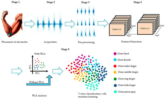
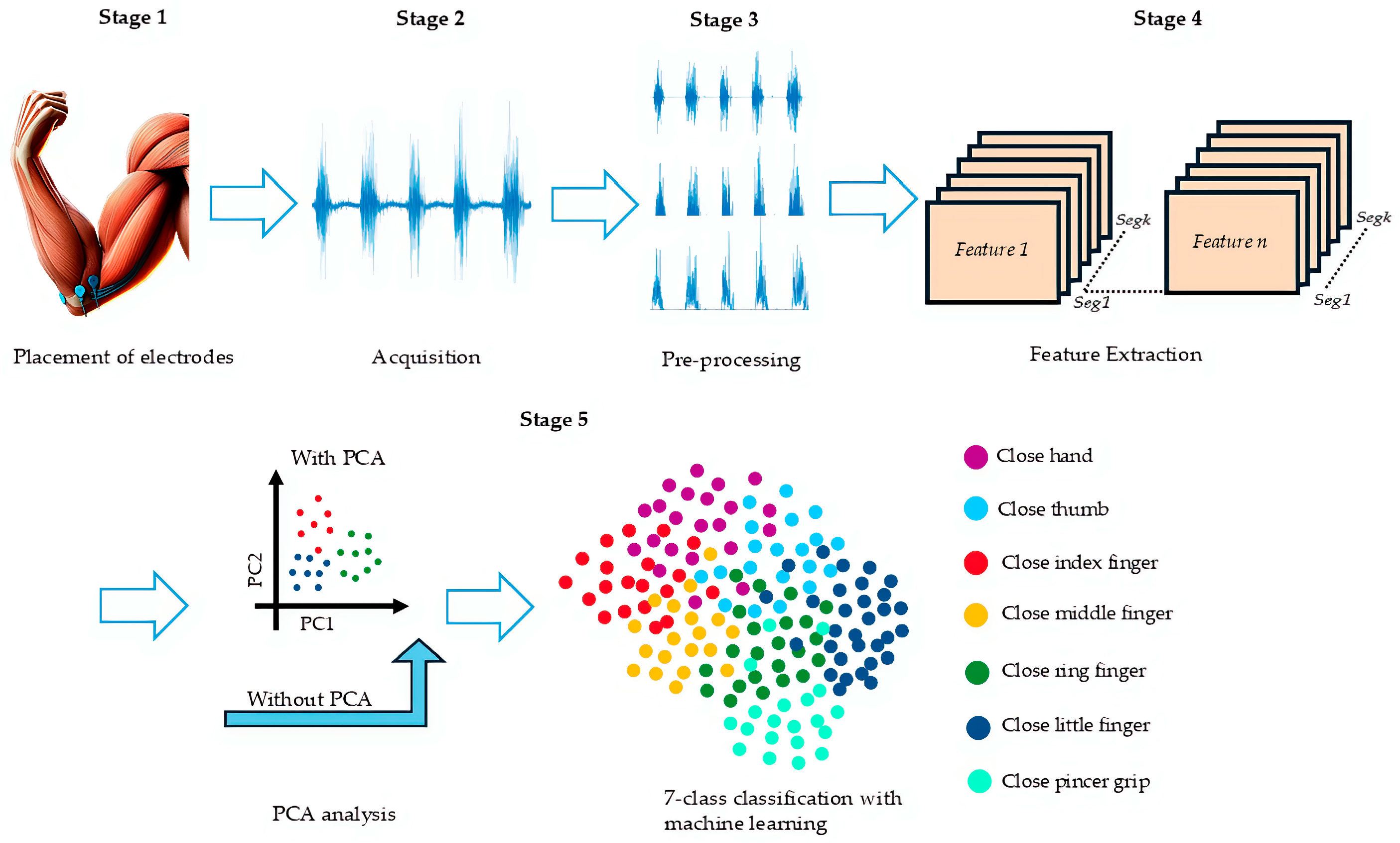
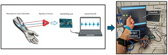
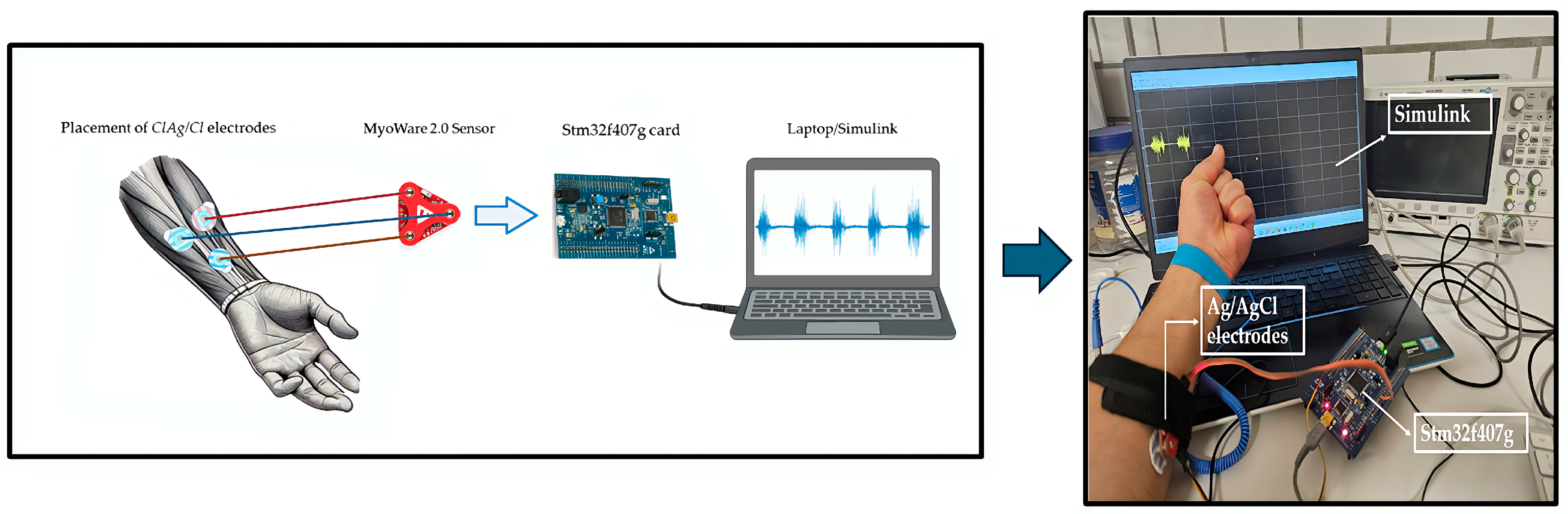
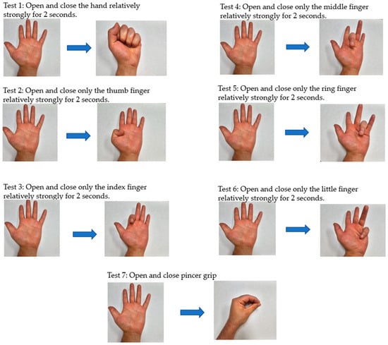
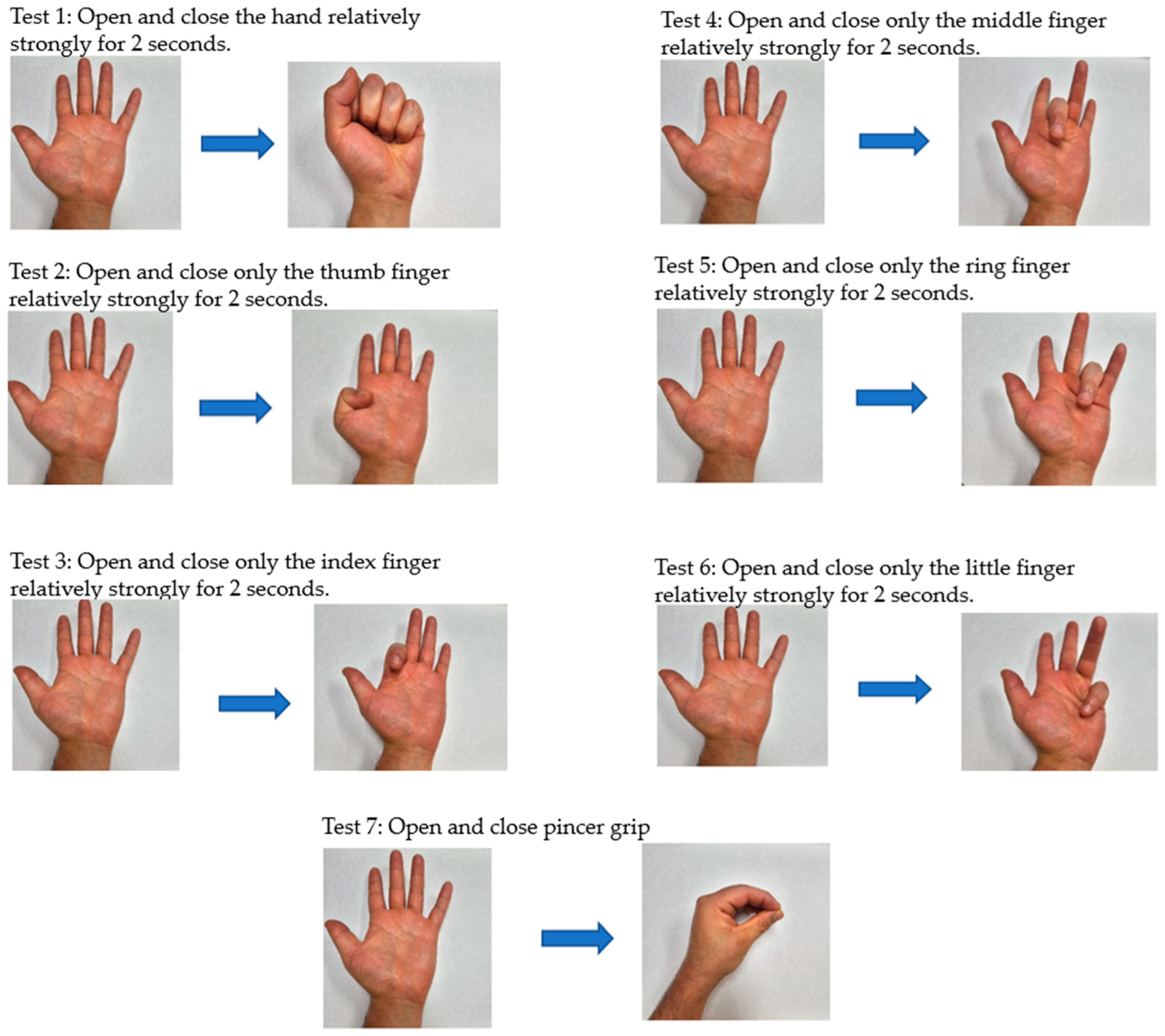
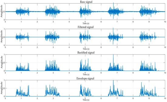
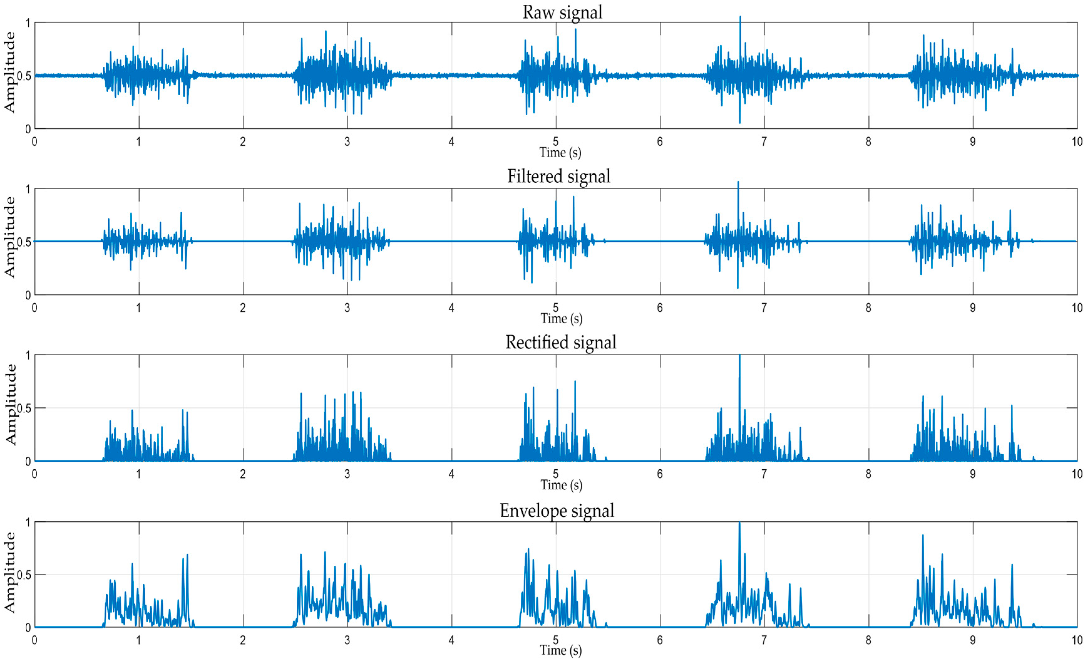
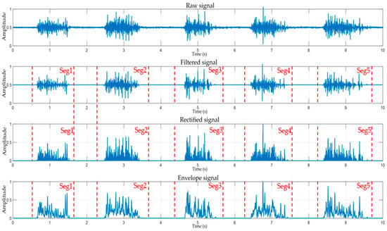
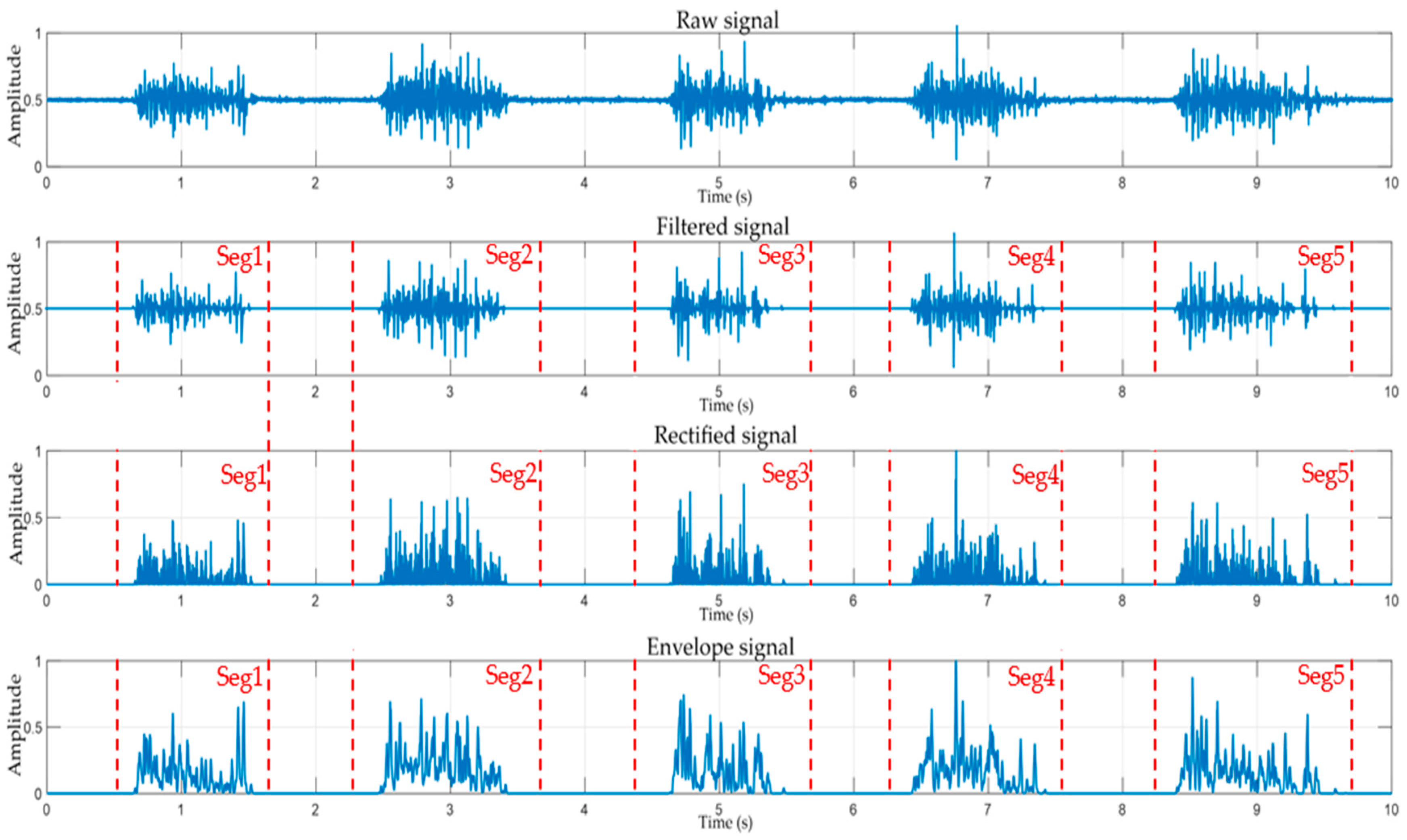
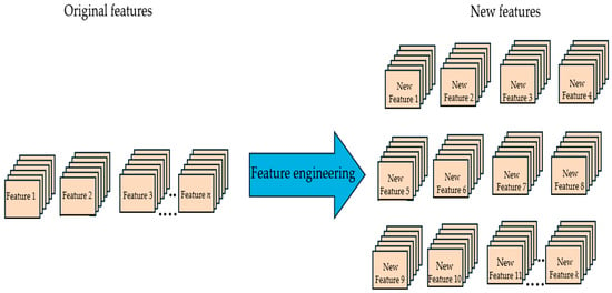
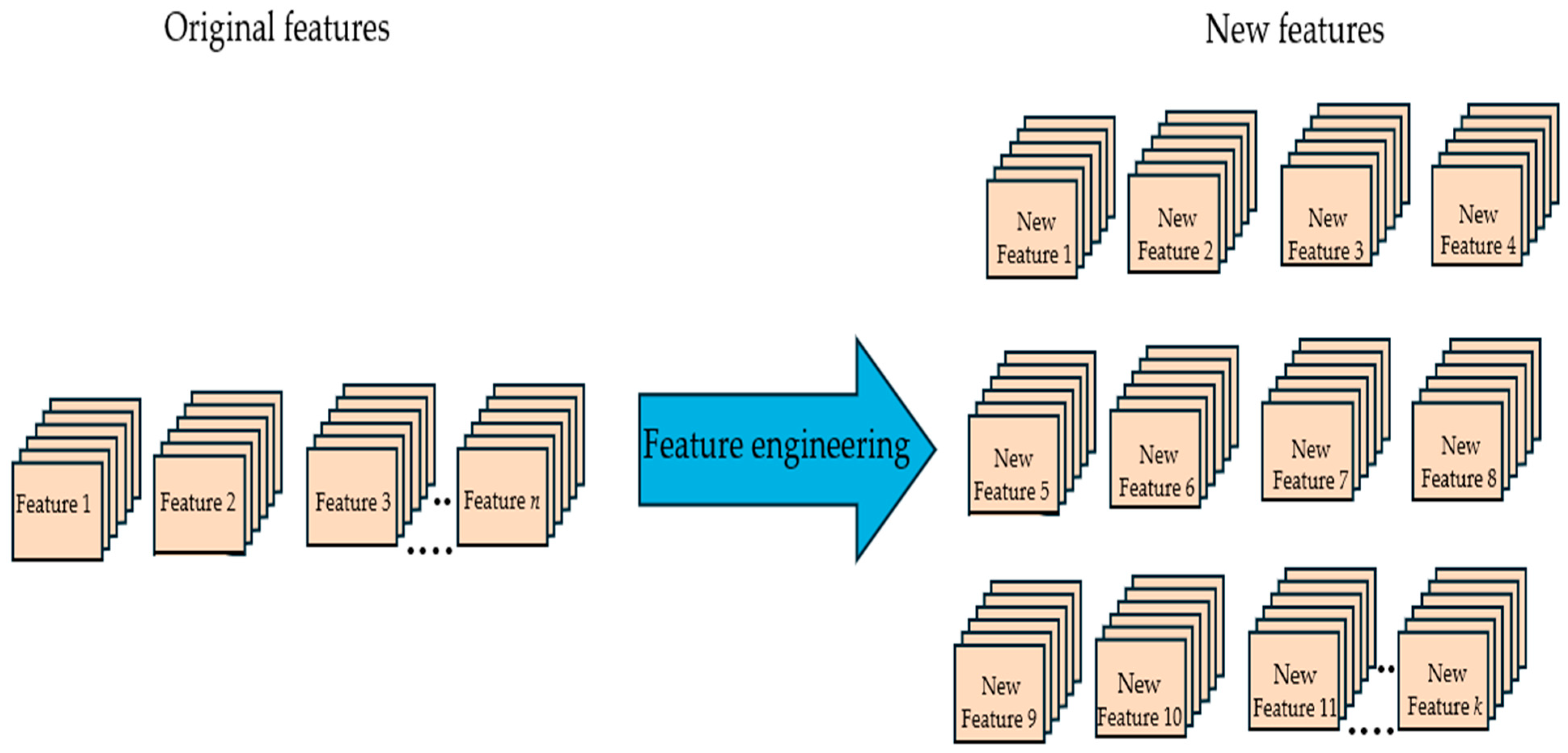
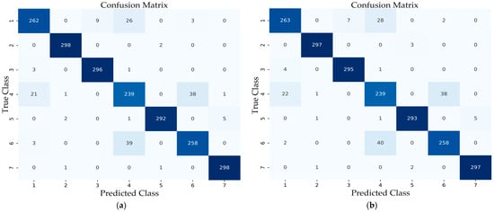
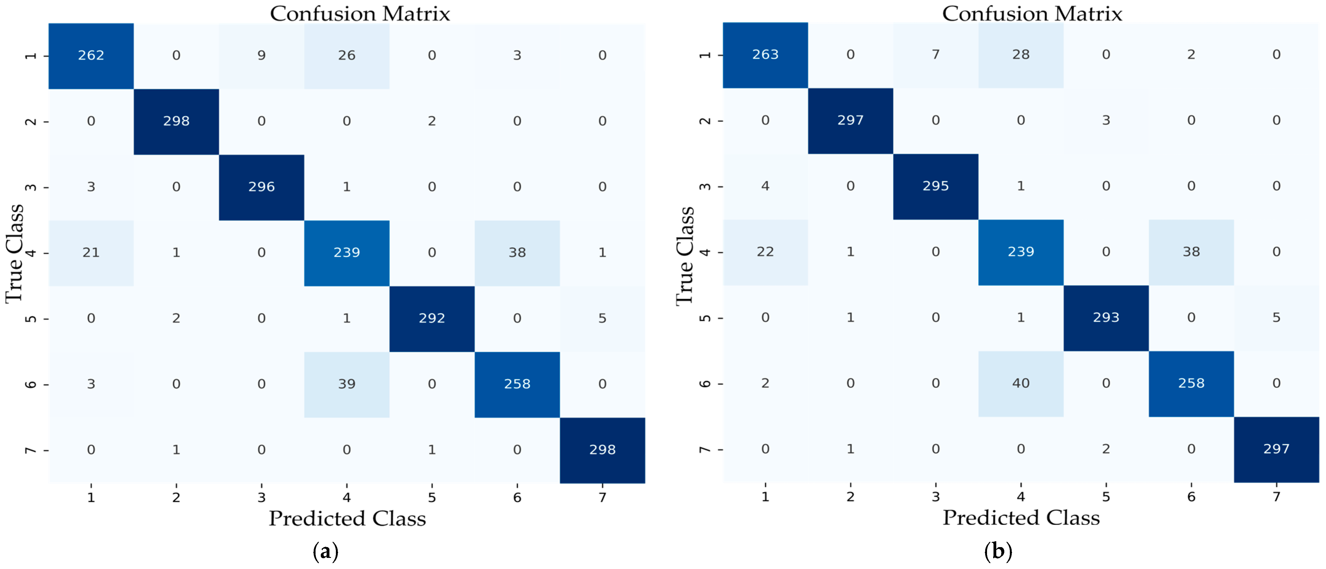
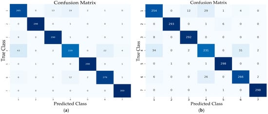
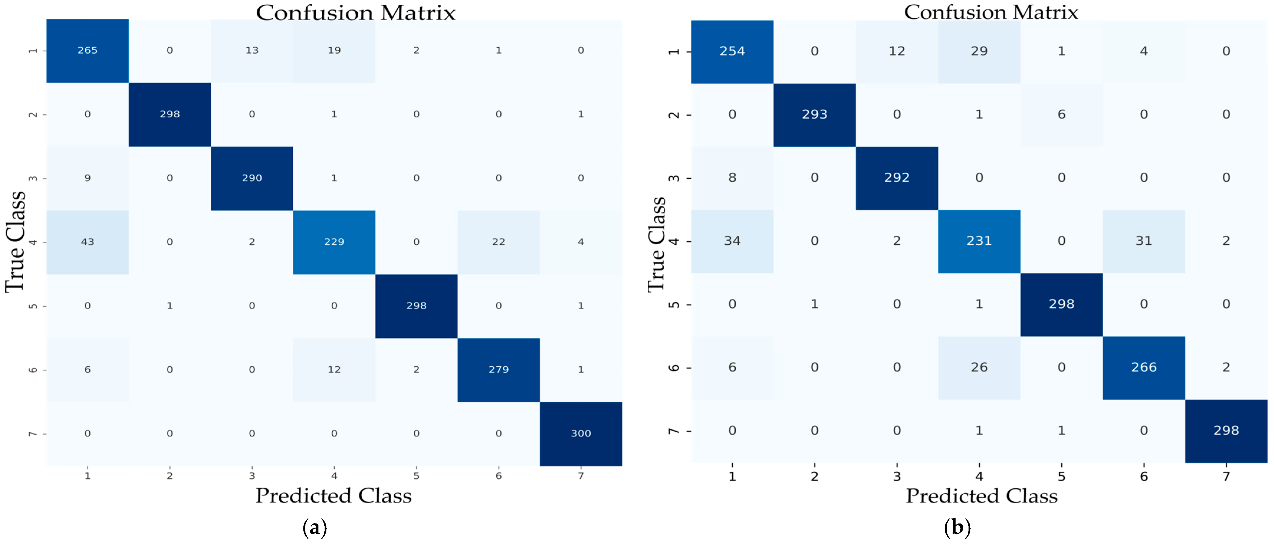
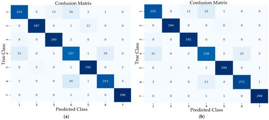
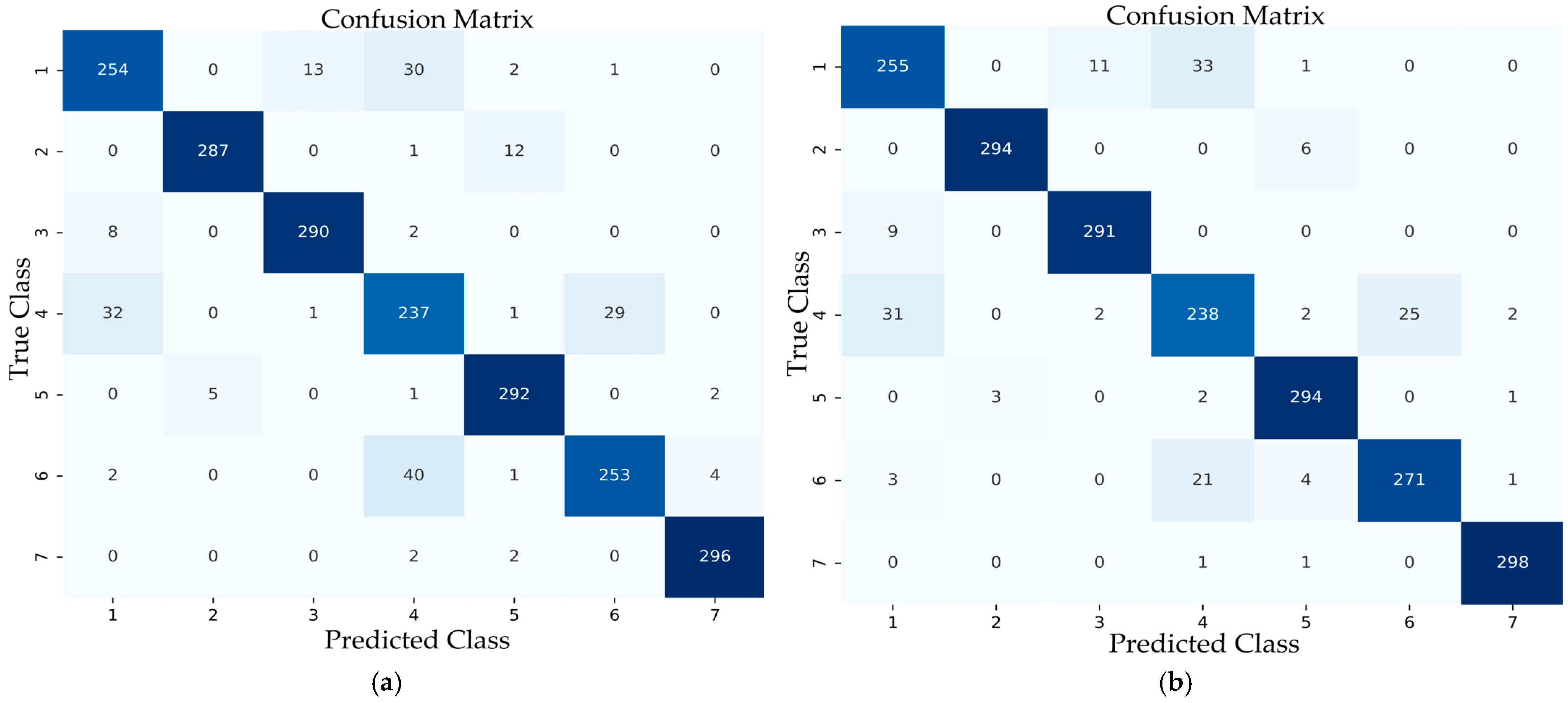

Disclaimer/Publisher’s Note: The statements, opinions and data contained in all publications are solely those of the individual author(s) and contributor(s) and not of MDPI and/or the editor(s). MDPI and/or the editor(s) disclaim responsibility for any injury to people or property resulting from any ideas, methods, instructions or products referred to in the content. |
© 2026 by the authors. Licensee MDPI, Basel, Switzerland. This article is an open access article distributed under the terms and conditions of the Creative Commons Attribution (CC BY) license.