


Abstract
Landslides are a common type of geological hazard, characterized by sudden onset, high destructiveness, and frequent occurrence, and are widely distributed in mountainous areas with complex terrain. In recent years, due to extreme weather and intensified human activities, both the frequency and intensity of landslide disasters in China have increased significantly, posing serious threats to human life, property, and socio-economic development. Although various methods for landslide susceptibility assessment have been proposed, the accuracy of existing models still needs improvement. In this context, this study takes the landslide-prone Dongchuan District of Kunming City, Yunnan Province, as a case study and proposes a coupled model that integrates an autoencoder and a feedforward neural network (AuFNN). The model uses the autoencoder to extract low-dimensional and highly discriminative feature representations, which are then used as input to the feedforward neural network to perform landslide susceptibility assessment. To evaluate the effectiveness of the proposed model, it is compared with four commonly used models, Support Vector Machine (SVM), Random Forest (RF), XGBoost, and Feedforward Neural Network (FNN), based on performance metrics such as the ROC curve, recall, and F1 score. The results indicate that the AuFNN model provides an alternative representation learning framework and achieves performance comparable to that of established machine learning models in landslide susceptibility assessment, as reflected by similar AUC, accuracy, and F1 score values.
1. Introduction
Landslides refer to the downward movement of soil and rock masses on a slope under the influence of gravity, triggered by natural or human-induced factors along a specific weak zone or surface [1,2]. They are characterized by wide distribution, high frequency, and severe destructiveness, causing billions of dollars in economic losses annually and posing serious threats to human lives, property, and socio-economic development [3,4,5,6]. Under such circumstances, it is imperative to adopt effective measures for landslide susceptibility assessment to mitigate potential hazards. Research on landslide susceptibility can be traced back to the 1960s, when early studies, such as those by Valiant, were among the early efforts to investigate the conditions and spatial characteristics of landslide occurrence [7]. Subsequently, Dobrovolny analyzed geological data from the Anchorage area to delineate stable and unstable zones, and his work contributed to the early development of landslide susceptibility assessment [8]. Over the past decades, researchers worldwide have developed a variety of models for landslide susceptibility assessment. These models can generally be categorized into two types: qualitative and quantitative [9,10]. Qualitative assessments are mainly based on knowledge-driven models, relying on expert knowledge and experience [10,11]. Common approaches include expert scoring methods, Analytic Hierarchy Process (AHP), and fuzzy logic [12,13,14]. For example, Silvana Moragues applied AHP to assess landslide susceptibility in northern Argentina [15] while Siamak Baharvand used fuzzy logic and GIS to conduct susceptibility assessments in northwestern Iran [16]. These methods have the advantage of leveraging expert insights, but also suffer from drawbacks such as heavy workload, strong subjectivity, and dependence on the expert’s cognitive scope. In contrast, quantitative assessments focus more on data-driven models [11]. These methods utilize large volumes of measured data and apply statistical or machine learning techniques to evaluate landslide susceptibility. Common models include the certainty factor model, information value model, frequency ratio, and various machine learning algorithms.
With the rapid advancement of artificial intelligence, especially the maturation of machine learning techniques, machine learning has shown significant advantages in landslide susceptibility assessment [17]. Compared with traditional statistical methods, machine learning models do not require strict assumptions about data distributions and can flexibly handle complex nonlinear relationships, thereby supporting more accurate landslide predictions [18]. At present, widely used machine learning models in this field include SVM, Random Forests (RF), XGBoost, Artificial Neural Networks (ANN), Multilayer Perceptrons (MLP), and various ensemble learning methods [19,20,21,22]. For example, Yu generated a landslide susceptibility map using SVM; Shahrzad Nikoobakht implemented a convolutional neural network (CNN) for susceptibility assessment in northeastern Iran; Zhang used XGBoost to assess landslide susceptibility in Fengjie, Chongqing; and Chang applied SVM and RF by considering the internal heterogeneity of slope units in Chongyi County [19,22,23,24]. Hossein Moayedi adopted a particle swarm optimization (PSO)-based ANN to produce a susceptibility map, while Nirdesh Sharma developed a high-resolution nationwide landslide susceptibility map in India using imbalance-aware ensemble machine learning methods, significantly improving prediction accuracy and generalization [25,26].
Owing to their ability to capture complex nonlinear relationships and learn representative features, machine learning methods have been widely applied in landslide susceptibility assessment [27]. These models can extract landslide-relevant features from complex and large datasets, thus improving the accuracy of susceptibility assessments. However, single models often face challenges such as overfitting and factor uncertainty, limiting their adaptability and generalizability. Most existing studies depend on high-dimensional evaluation factors with substantial feature redundancy; however, the explicit integration of feature representation learning into susceptibility modeling has received limited attention. Consequently, recent studies have gradually shifted from single models to coupled models [28,29]. By integrating the strengths of multiple algorithms, coupled models can more comprehensively capture landslide characteristics and enhance prediction accuracy and stability. A well-designed coupled model not only improves adaptability and generalization but also aligns prediction results more closely with real-world scenarios, increasing practical value and application prospects [30].
Based on this, the present study proposes a coupled model integrating an autoencoder and a feedforward neural network (AuFNN) for landslide susceptibility assessment. Autoencoders are capable of automatically learning low-dimensional and highly discriminative feature representations, which effectively mitigate the impact of redundant information on predictive performance. The model utilizes an autoencoder to extract low-dimensional and highly discriminative feature representations, thereby eliminating the interference of redundant information in subsequent tasks, thereby addressing the limitations of existing methods in feature extraction and generalization capability.
2. Study Area and Data
2.1. Overview of the Study Area
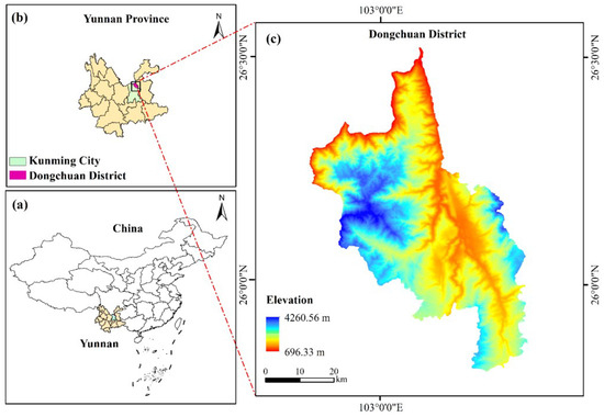
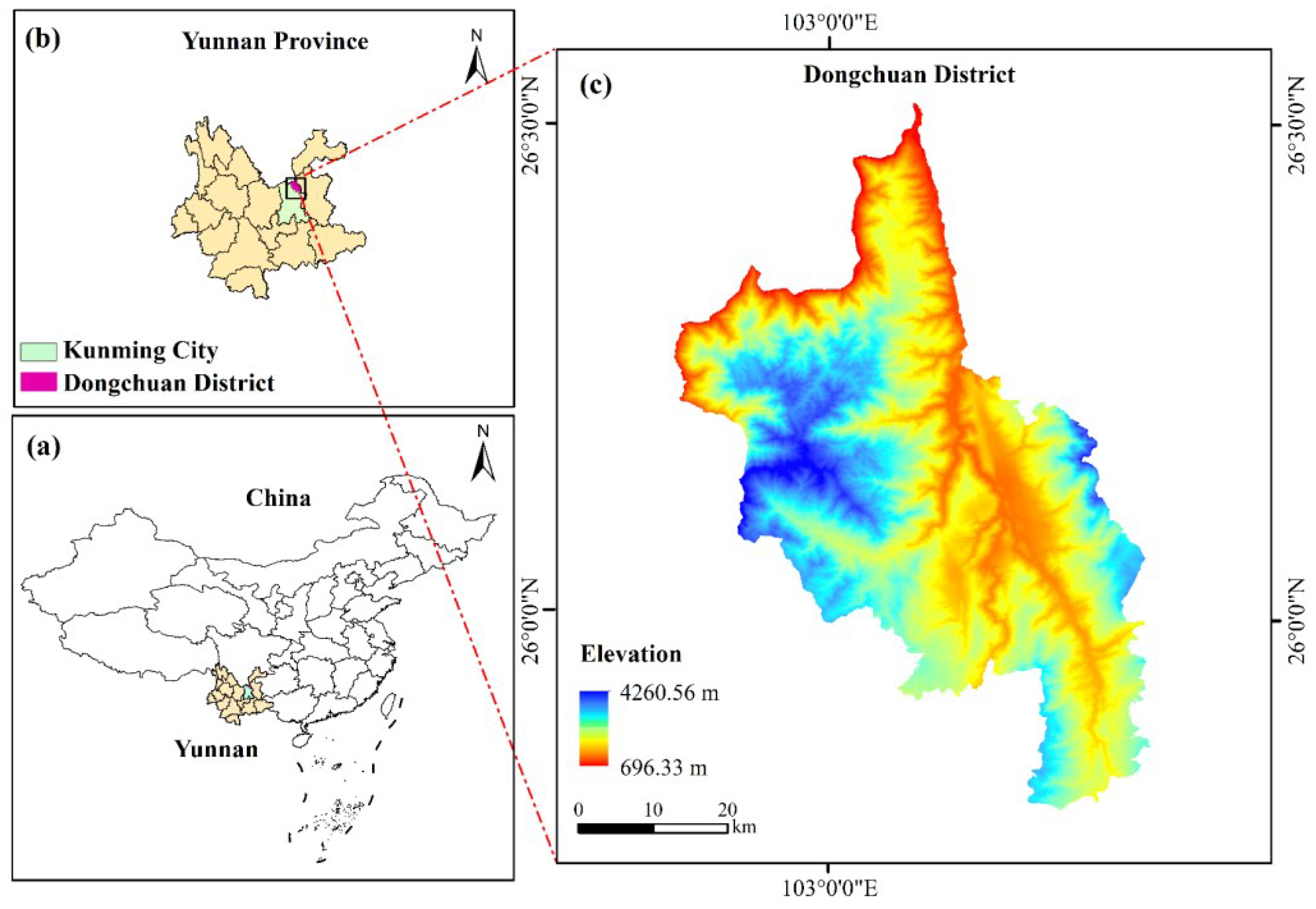
The study area is located in Dongchuan District, Kunming City, Yunnan Province, between 102°47′–103°18′ E and 25°57′–26°32′ N. It borders Huize County of Qujing City to the east, Xundian Hui and Yi Autonomous County to the south, Luquan Yi and Miao Autonomous County to the west, and Qiaojia County of Zhaotong City to the north. Across the Jinsha River, it faces Huili County and Huidong County in Liangshan Prefecture, Sichuan Province. The total area covers 1865.8 square kilometers, and the specific geographic location is shown in Figure 1.
Figure 1.
Overview Map of the Study Area. (a) Location of Yunnan Province within China; (b) Location of Dongchuan District within Yunnan Province; (c) Elevation map of Dongchuan District Note: All maps are projected in the CGCS2000 coordinate system with the 3° Gauss–Krüger projection. Landslides in the study area are mainly controlled by complex terrain conditions, lithology, and rainfall, which makes Dongchuan a representative and suitable test site for landslide susceptibility modeling.
2.2. Data Sources and Dataset Description
The data used in this study include landslide disaster data, digital elevation model (DEM) data, and road and river system data. Detailed information is presented in Table 1.
Table 1.
Data Sources.
The DEM data were obtained from the Airborne Geophysics and Remote Sensing Center of the China Geological Survey and were used to extract topographic and geomorphological factors of the study area. Remote sensing imagery from the same source was employed to derive the Normalized Difference Vegetation Index (NDVI). Landslide inventory data were also collected from the Airborne Geophysics and Remote Sensing Center of the China Geological Survey and were used to construct landslide and non-landslide samples. Land use information was obtained from the global land cover dataset with a spatial resolution of 30 m, which was developed and released under the organization of the Ministry of Natural Resources of China. Rainfall data were downloaded from the NOAA website based on meteorological station observations from Dongchuan District and surrounding areas, and kriging interpolation was applied to generate gridded precipitation data.
ArcGIS 10.7 was used to extract the evaluation factors for each slope unit, which served as input variables for the susceptibility models. Based on 178 historical landslide scar data in Dongchuan District, slope units with landslide occurrences were labeled as 1, and those without were labeled as 0. When the slope units were delineated using a hydrological analysis method, the number of units with landslides was 226, and those without landslides were 896. When the TFPF-SU method was used to delineate the slope units, the number of landslide units was 431, and the number of non-landslide units was 3974 [31]. The dataset was divided into training and testing sets at a ratio of 7:3. Given the class imbalance in the dataset, the Synthetic Minority Over-sampling Technique (SMOTE) was applied to oversample the landslide class in the training set, resulting in a 1:1 ratio between landslide and non-landslide samples. This strategy aims to reduce the adverse effects of class imbalance on model predictive performance.
2.3. Evaluation Factor Analysis
In the process of extracting evaluation factors, all datasets were standardized to a uniform format with a spatial resolution of 30 m and were stored in raster format. All data shared a consistent coordinate system, CGCS2000, with a projection based on the 3° Gauss-Krüger zone division, and used the 1985 National Height Datum as the elevation reference. The slope unit serves as the spatial carrier of evaluation factor information in this study and is the fundamental unit for expressing the evaluation factors. After extracting the evaluation factors, their raster-based representations were transformed to the slope unit scale. Two primary methods were used to extract the evaluation factors within each slope unit: the mean value method and the area dominance method, which are applied as follows: (1) Mean Value Method: For continuously distributed factors in raster format that exhibit local similarity, such as elevation, profile curvature, NDVI, etc., the mean value of all raster cells within a slope unit was calculated and used as the evaluation factor for that unit. (2) Area Dominance Method: For categorical factors such as lithology and land use, the category occupying the largest area within a slope unit was identified and assigned as the categorical value of the corresponding evaluation factor for that unit.
2.3.1. Geomorphological Factors
- (1)
- Elevation (m)
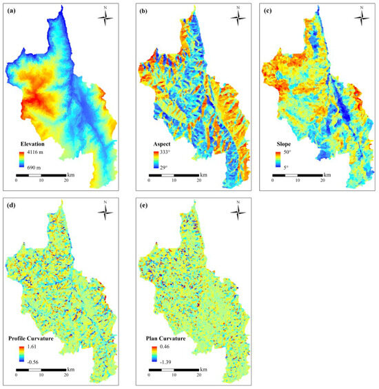
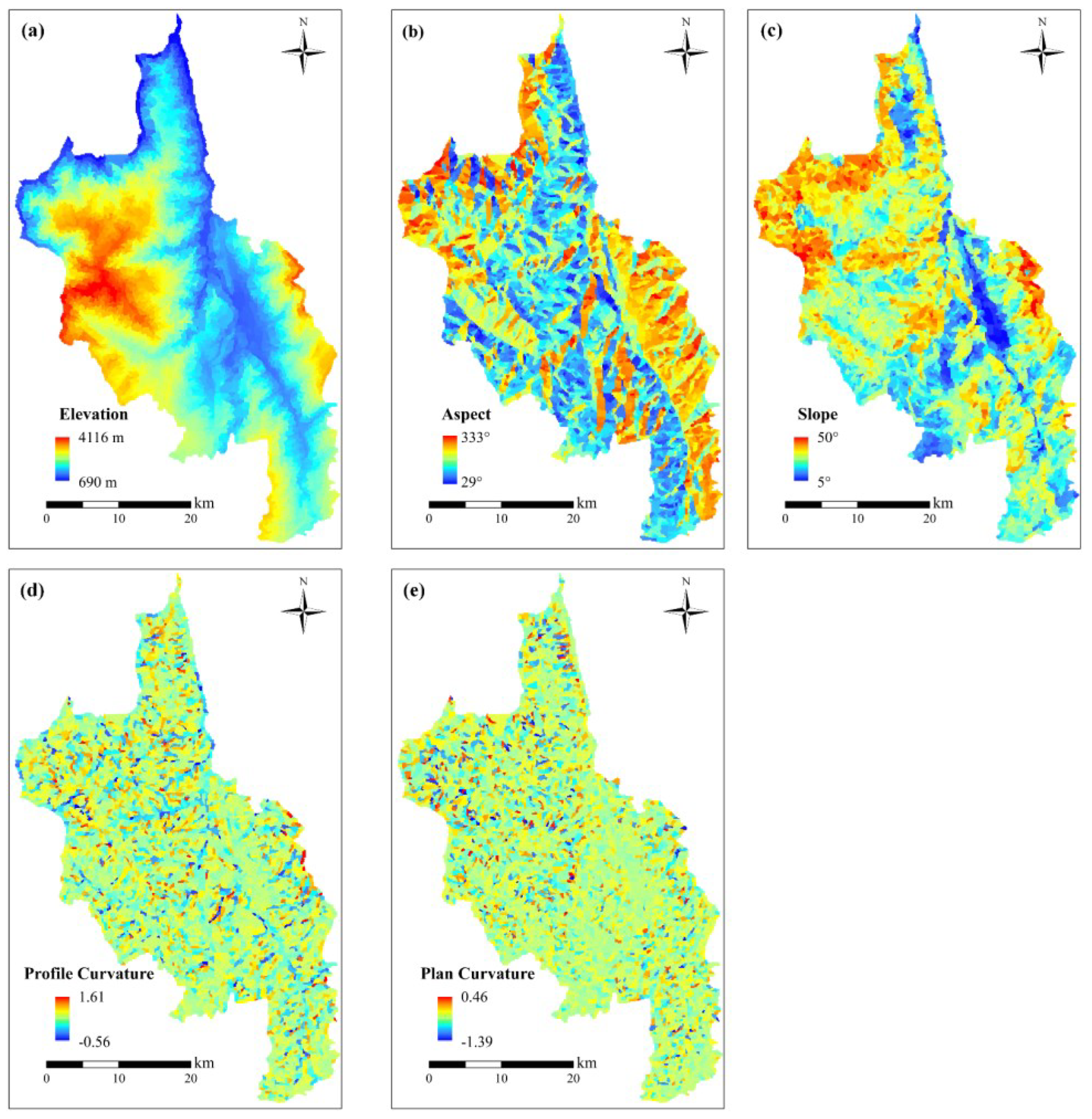
Elevation refers to the vertical distance of a point from the absolute datum, also known as absolute elevation. It is an important factor influencing the occurrence of landslides, closely related to the exposure conditions of rock and soil, vegetation coverage, and the intensity of human activities. Within specific elevation ranges, higher elevations tend to exhibit denser vegetation cover, fewer human disturbances, and more stable surface materials, thereby reducing landslide susceptibility. In contrast, lower elevation areas often experience frequent human activities, lower vegetation coverage, and looser surface materials, all of which contribute to higher landslide risk [32]. Therefore, understanding the spatial distribution of elevation in the study area is crucial for landslide risk assessment. Figure 2 illustrates the elevation distribution within the study area.
Figure 2.
The topographic and geomorphological factors of the study area: (a) Elevation, (b) Aspect, (c) Slope, (d) Plan curvature, (e) Profile curvature.
The elevation of slope units in Dongchuan District ranges from 690 to 4116 m. As shown in Appendix A, slope units with elevations between 1216 and 1859 m are more prone to landslides.
- (2)
- Slope (°)
Slope gradient represents the steepness of the terrain surface and is defined as the ratio between vertical elevation change and horizontal distance [2]. It not only reflects the inclination of the land surface but also affects the flow of surface materials and energy transfer efficiency. Areas with steeper slopes are more susceptible to gravitational movement of surface materials, increasing the likelihood of landslides. In contrast, flatter areas generally exhibit lower landslide risk. Figure 2 shows the distribution of slope gradients across the study area.
The slope gradient of slope units in Dongchuan District ranges from 5° to 49.2°. According to Appendix A, slope units with gradients between 25.26° and 32.52° are most favorable for landslide occurrence.
- (3)
- Aspect
Aspect refers to the compass direction that a slope faces. Different aspects experience varying exposure to sunlight and wind, which in turn affect soil moisture retention and vegetation growth, thereby influencing the spatial distribution of geographic features. These differences can significantly impact rock weathering, geomorphological changes, and landslide development. Figure 2 illustrates the aspect distribution in the study area.
As shown in Appendix A, slope units with southwest, west, northwest, and northeast aspects are more favorable for landslide occurrence.
- (4)
- Plan Curvature
Plan curvature refers to the degree of curvature of the terrain in the horizontal direction. Negative values indicate concave surfaces, while positive values indicate convex surfaces. Figure 2 presents the spatial distribution of plan curvature in the study area.
The plan curvature of slope units in Dongchuan District ranges from −1.39 to 0.46. According to Appendix A, landslides are more likely to occur when plan curvature values fall between 0.03 and 0.07.
- (5)
- Profile Curvature
Profile curvature describes the curvature of the terrain in the vertical direction. Positive values indicate a concave profile (i.e., downward-curving surface), while negative values indicate a convex profile (i.e., outward-curving surface). Figure 2 shows the distribution of profile curvature in the study area.
The profile curvature of slope units in Dongchuan District ranges from −0.56 to 1.61. As indicated in Appendix A, landslide susceptibility increases when profile curvature values are between 0.1 and 0.19.
2.3.2. Geological and Soil Factors
- (1)
- Lithological units
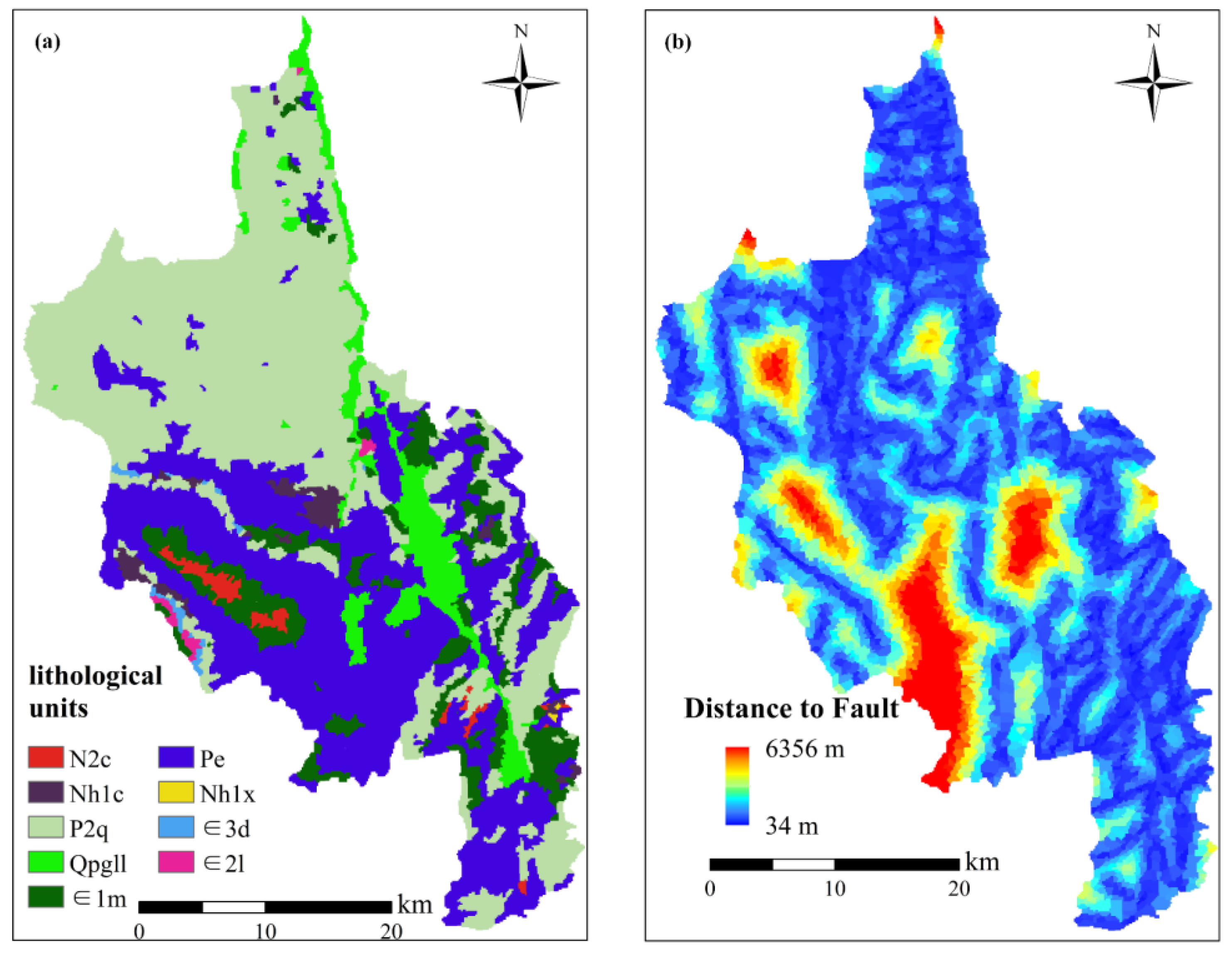
Rock type determines the degree of weathering and resistance to weathering of rock and soil masses, thereby affecting slope deformation and stability [33,34]. Due to variations in geological age, chemical composition, mineral content, and physicochemical properties, different lithological strata have significantly different impacts on geological hazards [14,33]. Figure 3 shows the spatial distribution of lithology in the study area.
Figure 3.
The soil and geological factors of the study area: (a) lithological units, (b) Distance to fault. Note: Lithology represents the integrated characteristics of rock material composition, structural features, genesis, and mechanical properties, and directly reflects the material attributes of strata as well as their controlling effects on geological processes and engineering stability. (classified into 0–50 m, 50–100 m, 100–150 m, 150–200 m, and >250 m). (a) Spatial distribution of lithological units in the study area. Different colors represent distinct lithological groups: N2c denotes weak rock group; Nhlc denotes hard rock group; P2q denotes relatively hard rock group; Qpgl1 denotes extremely weak rock group; E1m denotes relatively weak rock group; Pe denotes relatively hard to hard rock group; Nhlx denotes hard rock group interbedded with weak layers; E3d denotes relatively hard rock group interbedded with weak layers; and E21 denotes relatively weak to relatively hard rock group. The symbol “∈” indicates stratigraphic units belonging to a specific geological epoch.
According to Appendix A, slope units composed of moderately soft to moderately hard rocks and relatively weak rock formations are more prone to landslides.
- (2)
- Distance to Fault (m)
Generally, areas closer to faults tend to have a higher landslide density. Faulting and fracturing processes often form free surfaces or gullies, providing favorable conditions for landslide initiation. Dongchuan District is located in the Xiaojiang Fault Zone, where seismic activity is frequent. Areas near faults tend to have more fragmented geological structures and lower slope stability, making them more susceptible to landslides [35,36]. Figure 3 shows the distribution of fault proximity within the study area.
The distance to fault for slope units in Dongchuan District ranges from 29 to 333 m. According to Appendix A, slope units located within 0–200 m of a fault are most susceptible to landslides [2].
2.3.3. Meteorological and Hydrological Factors
- (1)
- Annual Precipitation (mm)
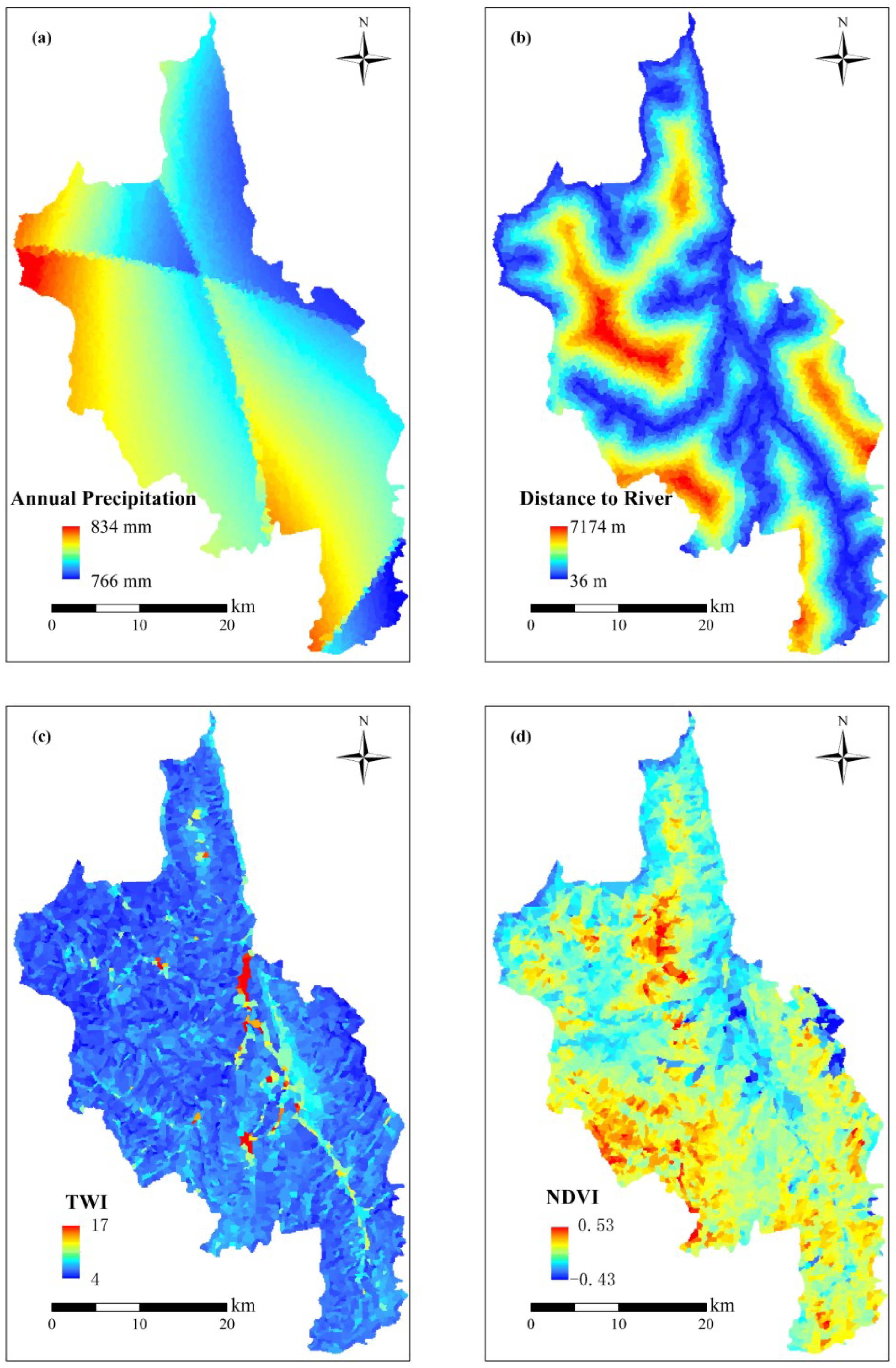
When rainwater infiltrates a slope, it increases the weight of the slope mass, potentially causing the downslope force to exceed a critical threshold and triggering landslides. During the rainy season, increased precipitation often intensifies the frequency and severity of landslide events. Heavy rainfall can result in water accumulation and flooding due to inadequate infiltration, continuously eroding the slope and reducing its stability, ultimately leading to landslides. Figure 4 illustrates the distribution of annual precipitation in the study area.
Figure 4.
The meteorological and hydrological factors: (a) Annual precipitation, (b) Distance to river, (c) TWI, (d) NDVI.
In Dongchuan District, the annual precipitation of slope units ranges from 766 to 834 mm. According to Appendix A, slope units with precipitation between 785–791 mm and 817–834 mm are more prone to landslides.
- (2)
- Distance to River (m)
River erosion and fluctuations in the groundwater level can weaken slope stability. The rivers in Dongchuan District have strong erosive forces due to their rapid flow, especially during the rainy season, making slopes near rivers more susceptible to landslides. Figure 4 shows the distribution of distance to rivers in the study area.
The distance to rivers for slope units in Dongchuan District ranges from 36 to 7174 m. According to Appendix A, landslides are more likely to occur in areas close to rivers (0–1000 m).
- (3)
- Topographic Wetness Index (TWI)
The Topographic Wetness Index reflects the influence of topography on runoff direction and accumulation, quantifying its control over hydrological processes. A higher TWI indicates greater soil moisture content, which increases the likelihood of the soil reaching saturation and thus the risk of landslides. Figure 4 presents the spatial distribution of TWI in the study area.
In Dongchuan District, the TWI values for slope units range from 4 to 17. According to Appendix A, areas with higher TWI values (7.34–11.97) are more susceptible to landslides.
- (4)
- Normalized Difference Vegetation Index (NDVI)
NDVI is an indicator used to assess vegetation cover on the surface. Its values range from −1 to 1, with higher values indicating denser vegetation cover. Vegetation plays a crucial role in preventing landslides by reducing soil erosion and enhancing slope stability. Areas with sparse or low vegetation cover are more prone to landslides. Figure 4 shows the spatial distribution of NDVI in the study area.
In Dongchuan District, NDVI values for slope units range from −0.43 to 0.53. According to Appendix A, slope units with lower NDVI values are more likely to experience landslides.
2.3.4. Human Activity Factors
- (1)
- Land Use
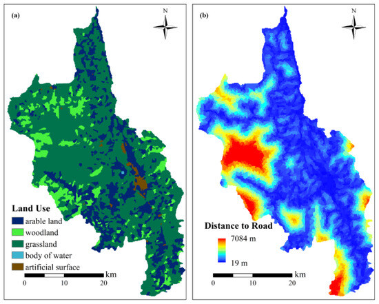
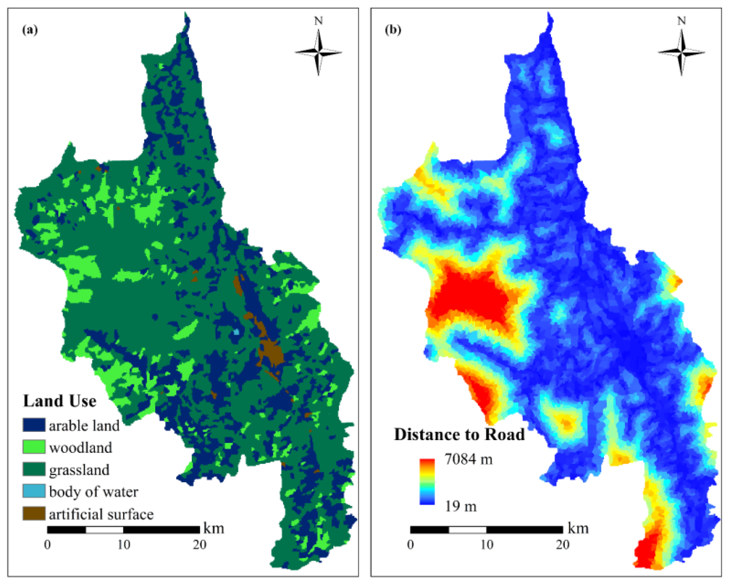
Different land use types directly influence the likelihood of landslides by altering the stability and degree of disturbance to slopes. For instance, forestry land, with its dense vegetation cover, enhances slope stability and thereby reduces the risk of landslides. In contrast, land used for agriculture and residential purposes often leads to significant disturbance and damage to slope surfaces, including the disruption of soil and rock layers, which weakens overall slope stability and increases the probability of landslides. Figure 5 illustrates the spatial distribution of land use in the study area.
Figure 5.
Human activity factors: (a) Land use, (b) Distance to road.
According to Appendix A, slope units classified as artificial surfaces and cultivated land are most prone to landslides.
- (2)
- Distance to Roads (m)
As transportation infrastructure in the study area develops with technological and economic advancement, road construction has expanded significantly. During the construction process, extensive excavation and filling works can severely disrupt the natural stability of slopes. Moreover, inadequate drainage systems near roads can lead to surface water accumulation, further elevating the risk of landslides. Figure 5 shows the distribution of distances to roads within the study area.
In Dongchuan District, the distance from slope units to roads ranges from 19 to 7084 m. According to Appendix A, slope units located closer to roads (0–1000 m) are more likely to experience landslides.
3. Methods
3.1. Collinearity Test of Evaluation Factors
The Pearson correlation coefficient (R), first proposed by Karl Pearson, is a measure of the strength of the linear relationship between two variables [37]. Its absolute value is used to assess the degree of linear correlation, with larger absolute values indicating stronger correlations. The value of R ranges from −1 to 1. A value less than 0.3 indicates little to no correlation between variables; a value between 0.3 and 0.5 suggests a low level of correlation; and a value greater than 0.5 indicates a high level of correlation. When the correlation exceeds 0.5, one of the correlated variables is typically removed to reduce factor redundancy. The formula for calculating the Pearson correlation coefficient is as follows:
where and represent the mean values of the landslide-related factors, and and are the actual values of the two variables.
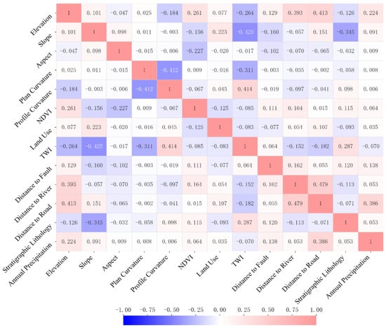
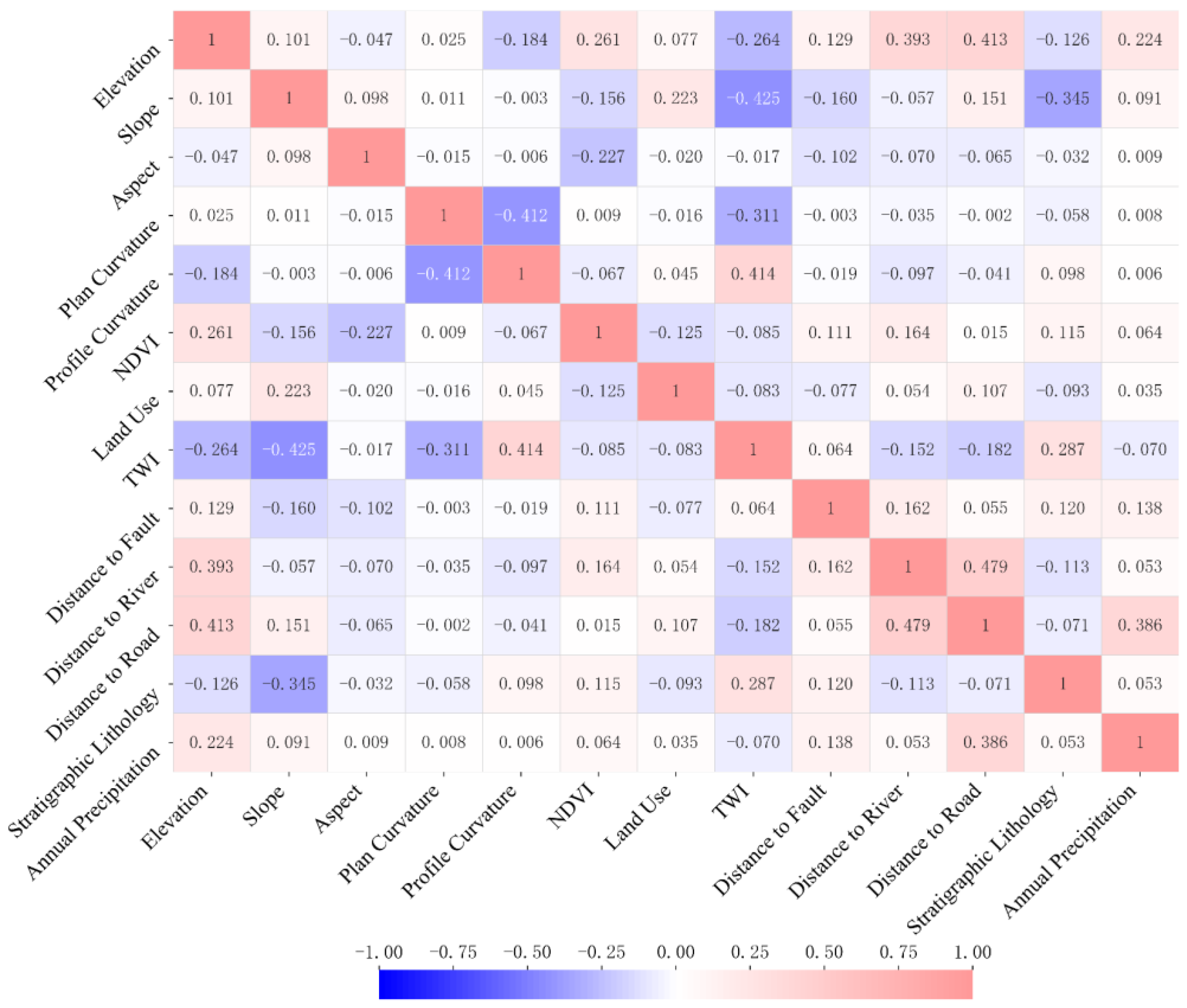
In this study, the values of each evaluation factor within the slope units were calculated using the ArcGIS platform, and the corresponding attribute table was exported for Pearson correlation analysis. Highly correlated factors were removed, and 13 evaluation factors were ultimately retained: aspect, distance to rivers, slope, distance to roads, distance to faults, profile curvature, land use, annual precipitation, plan curvature, normalized difference vegetation index (NDVI), elevation, topographic wetness index (TWI), and lithology. Figure 6 presents the Pearson correlation matrix among these 13 evaluation factors. Positive values in the legend indicate positive correlations, while negative values indicate negative correlations. As shown in Figure 6, some degree of correlation exists between different factors, but all retained factors in this study exhibit correlation values below the 0.5 threshold.
Figure 6.
Correlation Coefficient Matrix of Evaluation Factors.
3.2. Correlation Analysis Between Landslides and Evaluation Factors
In landslide susceptibility evaluation, researchers have proposed various nonlinear coupling methods—such as the information value method, weights of evidence method, and frequency ratio method—to characterize the relationship between landslides and environmental factors [19,38,39,40]. These methods help analyze how specific factors contribute to landslide occurrences. Based on previous studies, such as those conducted by Li Wenbin and others, which explored the impact of different nonlinear coupling approaches on the uncertainty of landslide susceptibility modeling, this study adopts the frequency ratio (FR) method to analyze the relationship between landslides and environmental factors [40]. The FR method categorizes environmental factors into two types: continuous and discrete. Continuous evaluation factors are divided into eight intervals using the natural breaks method, while discrete factors are classified based on their categorical attributes. For each classified environmental factor, the number of slope units with recorded landslides is counted within each interval, along with the total number of slope units in that interval. Two ratios are then calculated: the proportion of landslide-occurring slope units in a given interval relative to the total number of landslide slope units, and the proportion of slope units in that interval relative to the total number of slope units in the study area. The frequency ratio (FR) is derived from the ratio of these two proportions. A higher FR value indicates that the environmental conditions in that interval are more conducive to landslide occurrence. This method enables efficient identification of which environmental factors—and which specific intervals—are more likely to promote landslides, thereby providing a scientific basis for landslide susceptibility evaluation.
where represents an interval of a given environmental factor; is the number of slope units with landslides in interval; is the total number of slope units in interval; is the total number of slope units with landslides; and is the total number of slope units in the study area.
The information values of the conditioning factors in the study area are listed in Appendix A.
3.3. Slope Unit Delineation Method and Results
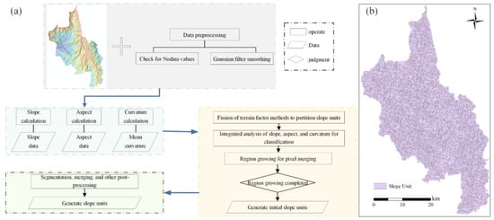
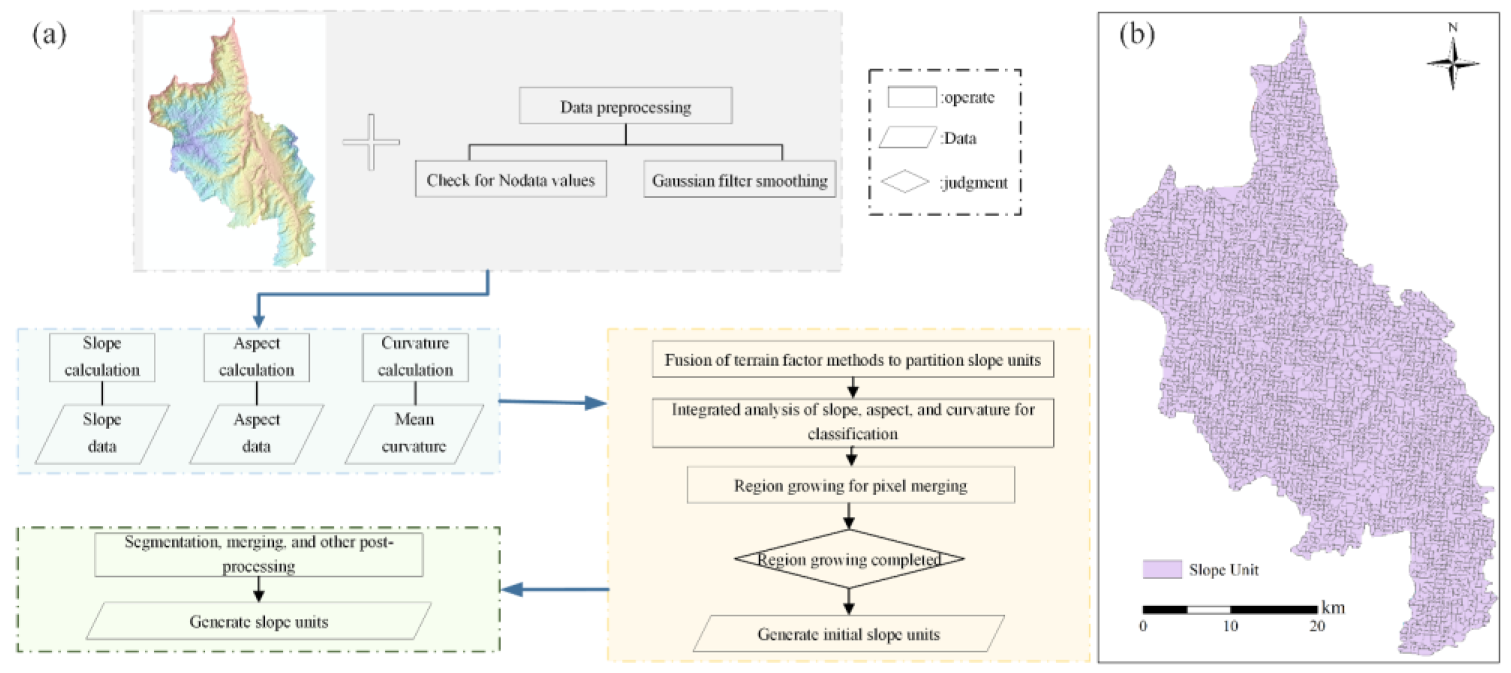
Compared with other types of mapping units, slope units better reflect the geomorphological and geological mechanisms underlying landslide development. In recent years, their application in landslide susceptibility assessment has grown significantly. In this study, a terrain-factor-fused and parameter-free slope unit delineation method (TFPF-SU) was employed to divide slope units in the Dongchuan District, which serve as the evaluation units for this research. The delineation steps of the slope units are illustrated in Figure 7a, and the resulting slope unit map is shown in Figure 7b.
Figure 7.
(a) TFPF-SU method flowchart for extracting slope units, (b) Slope units extracted.
3.4. Landslide Susceptibility Assessment Methods
3.4.1. Machine Learning Models
SVM is a supervised machine learning model that separates different classes of data by finding an optimal hyperplane and increasing the margin between classes to enhance the model’s ability to adapt to new data [41,42,43]. In practical applications, data are often nonlinearly separable, and SVM uses kernel methods to map the original nonlinear data into a higher-dimensional feature space, thus finding an appropriate hyperplane for classification. Kernel functions include linear kernels, polynomial kernels, and Radial Basis Function (RBF) kernels, among others. RBF has a strong nonlinear mapping capability and can control the mapping behavior of data using the hyperparameter gamma. Therefore, this study used the RBF kernel for SVM. SVM can also adjust the hyperparameter C to balance classification error and margin maximization. A larger C value reduces misclassification but may narrow the margin, increasing the risk of overfitting; a smaller C value increases classification tolerance, improving the model’s generalization ability but may lead to underfitting. In this study, an SVM model was constructed using Python version 3.9, and grid search was applied to optimize and select C and gamma, with C = 10 and gamma set to ‘scale’.
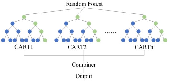
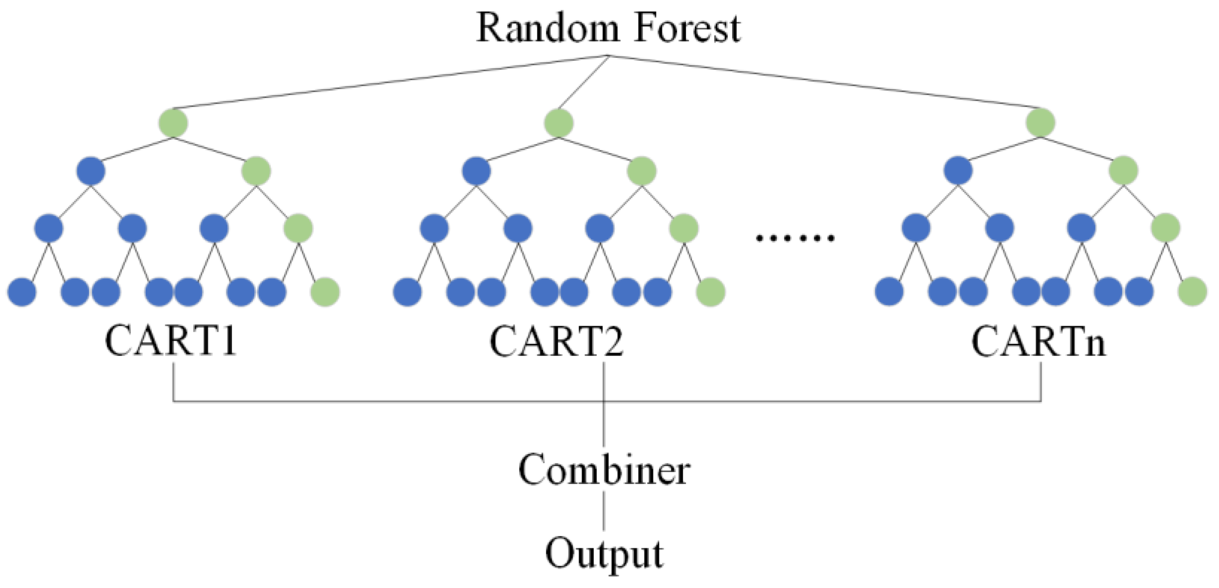
In 2001, Leo Breiman proposed a decision-tree-based ensemble learning algorithm, Random Forest (RF) [44]. RF combines the predictions of multiple decision trees to reduce variance, minimize overfitting risks, and improve the model’s overall generalization ability. In classification tasks, it uses a voting mechanism to determine the final result; in regression tasks, it averages the results from all decision trees. RF works through “bagging” and “random feature selection”. Bagging involves resampling the original training data with replacement to generate multiple different data subsets, each of which is used to train a decision tree. Training on different samples effectively reduces overfitting and enhances the model’s generalization ability. Parameters such as the number of decision trees (n_estimators), minimum samples required for node splits (min_samples_split), maximum number of features to consider for each split (max_features), minimum samples required for leaf nodes (min_samples_leaf), and tree depth (max_depth) all influence RF model accuracy. In this study, Python’s grid search was used to tune these parameters, resulting in n_estimators = 110, min_samples_leaf = 2, max_depth = 7, min_samples_split = 2, and max_features set to ‘sqrt’.The specific details are shown in Figure 8.
Figure 8.
Structure of Random Forest.
In 2014, Tianqi Chen and his team proposed a Boosting algorithm called XGBoost [45,46]. This algorithm constructs a strong learner by iteratively training weak learners (typically decision trees) and correcting the model based on each iteration’s errors. The objective function of XGBoost consists of a loss function and a regularization term, with the loss function measuring the prediction error and the regularization term controlling model complexity to prevent overfitting. XGBoost introduces feature sampling and data sampling techniques to increase model diversity and reduce the correlation between trees. It also allows custom loss functions for specific tasks. Hyperparameters such as learning rate (learning_rate), minimum sample weight for node splitting (min_child_weight), the number of base learners (n_estimators), feature sampling ratio (colsample_bytree), training data sampling ratio (subsample), and maximum tree depth (max_depth) affect model performance. In this study, the same parameter tuning method as RF was used, resulting in learning_rate = 0.002, min_child_weight = 1, max_depth = 6, subsample = 0.8, n_estimators = 100, and colsample_bytree = 0.7.
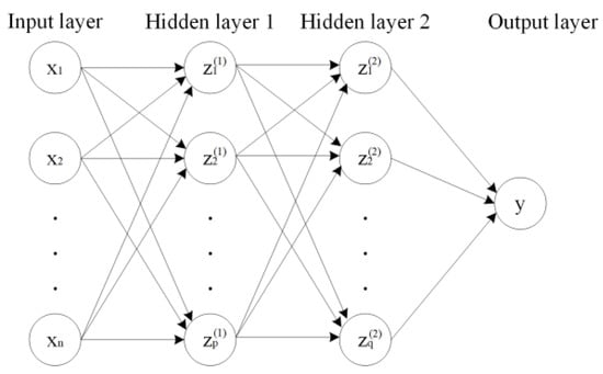
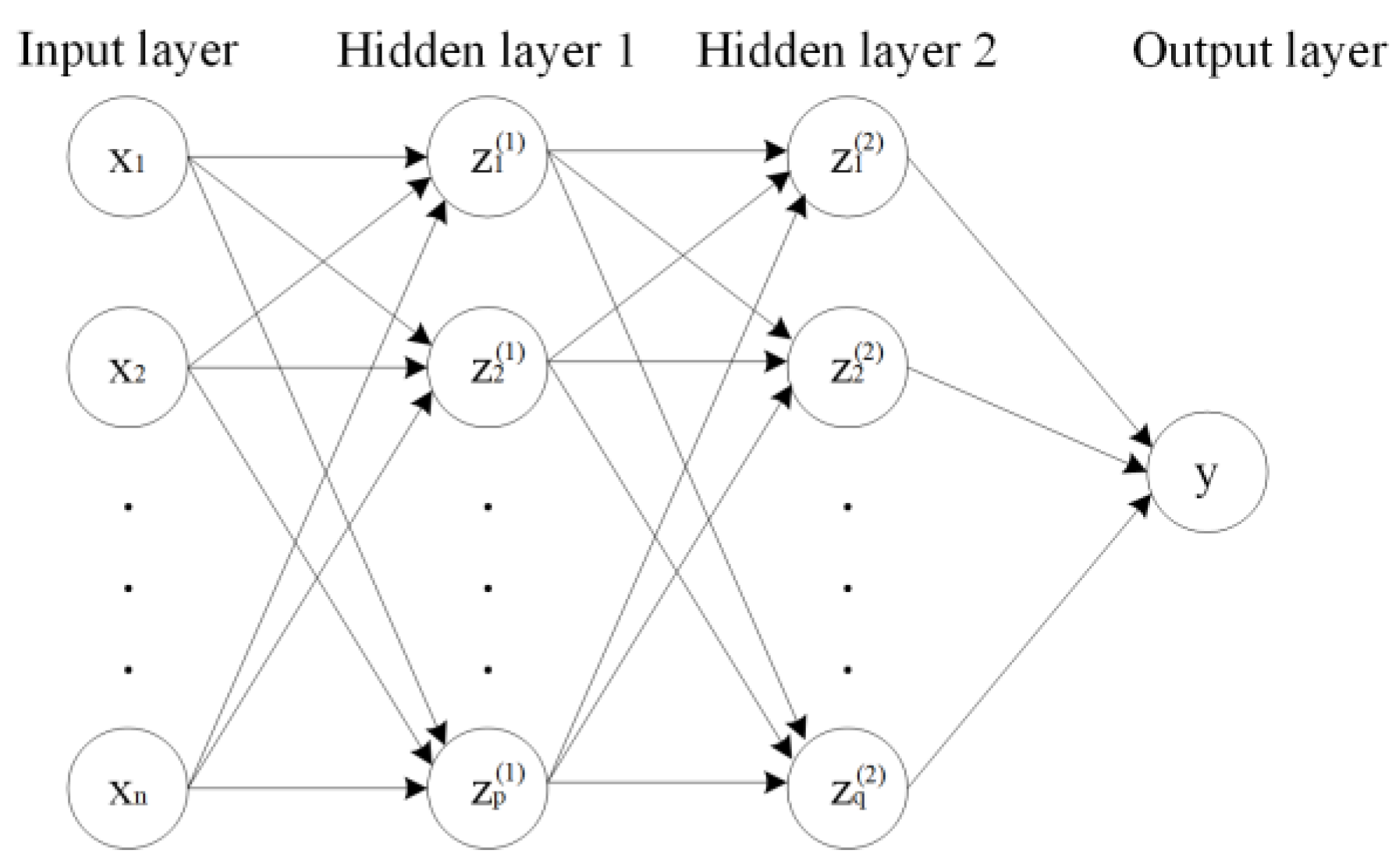
This study also employed a feedforward neural network (FNN) for landslide susceptibility assessment, consisting of an input layer, hidden layers, and an output layer [47]. The data is passed through the network layer by layer via weighted connections between neurons. Each neuron performs a weighted sum and a nonlinear transformation using an activation function, gradually transmitting information until the output layer generates a prediction. Common activation functions include Rectified Linear Unit (ReLU), Sigmoid, and Tanh. FNN performs forward propagation by passing input data through the network layer by layer, and after each layer’s weighted sum and activation function processing, it generates the predicted values at the output layer. These are compared with the true labels to calculate the loss function, which measures the model’s performance. The backpropagation algorithm calculates the gradients of the loss function with respect to weights and biases layer by layer, starting from the output layer. The gradient information is then used to update the weights and biases using gradient descent or other optimization algorithms, minimizing the loss function and improving model performance. In this study, a Python-based FNN model was constructed with one input layer, two hidden layers, and one output layer. The number of neurons in the hidden layers was set to 128, using the ReLU activation function in the hidden layers and the Sigmoid activation function in the output layer. The model was trained for 900 iterations with a learning rate of 0.002.The Structure of the Feedforward Neural Network are shown in Figure 9.
Figure 9.
Structure of the Feedforward Neural Network.
3.4.2. AuFNN
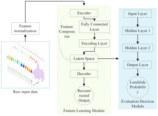
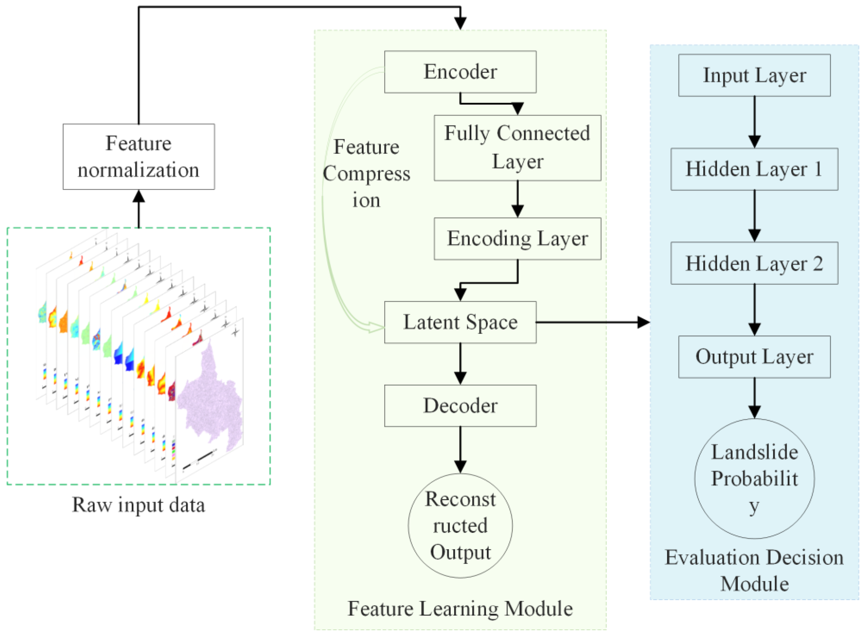
In landslide susceptibility assessment, to address the issues of model accuracy and redundancy of evaluation factors, this study proposes a coupling model integrating an autoencoder and a feedforward neural network (AuFNN). The input features of the model consist of the evaluation factors described in Section 2.3. The model is divided into two main modules: a feature learning module and an evaluation decision module. Its structure is shown in Figure 10.
Figure 10.
Structure of the AuFNN model.
The feature learning module in this study is centered on an autoencoder with an encoder–decoder structure. In the unsupervised learning mode, the autoencoder aims to extract low-dimensional and highly discriminative feature representations from the 13 evaluation factors (elevation, land use, NDVI, etc.) extracted in Chapter 2, in order to reduce the potential interference of redundant information in subsequent evaluation tasks. In this study, the encoder is designed as a two-layer fully connected neural network. The first layer is the hidden layer, with 128 neurons and a ReLU activation function to perform an onlinear transformation. The ReLU function has a significant advantage in alleviating the gradient vanishing problem and can effectively improve the stability of model training. The second layer is the encoding layer, responsible for compressing the data into an 11-dimensional latent space, also using the ReLU activation function to enhance the nonlinear mapping ability of the model. The decoder has a mirror-symmetric structure to the encoder. The decoder reconstructs the 11-dimensional latent features into a 128-dimensional intermediate layer, ultimately outputting 13-dimensional reconstructed data. The output layer uses the Sigmoid function to constrain the range of the reconstructed values, ensuring that the output data maintains consistency with the original data in terms of scale. The autoencoder is trained independently of the label data, minimizing the mean square error between the input and reconstructed data, thus learning the inherent distribution patterns of landslide-related factors and enhancing the generalization ability of the features.
The dimensionality of the encoding layer directly affects the final evaluation results. To select the optimal dimensionality, this study sets the encoding layer dimension from 1 to 13 and conducts 13 comparative experiments. Based on the accuracy of landslide susceptibility evaluation, the performance of the coupling model with different encoding layer dimensions is evaluated using indicators such as the Area Under the ROC Curve (AUC), accuracy, and recall rate. The experimental results show that the evaluation accuracy is highest when the encoding layer dimension is 11.
The evaluation decision module is based on a feedforward neural network (FNN), which takes the 11-dimensional latent space extracted by the autoencoder as input data. In this study, the FNN model is structured with one input layer, two hidden layers, and one output layer. Each hidden layer in the FNN contains 128 neurons, and the ReLU activation function is used to enhance the model’s ability to handle nonlinear relationships. The first hidden layer maps the 11-dimensional input to 128 dimensions to explore the local correlations between features. The second hidden layer maintains 128 dimensions to further integrate global nonlinear patterns and alleviate the gradient vanishing problem. The output layer uses the Sigmoid function to map the final result to the [0, 1] range, representing the landslide susceptibility probability of each slope unit.
To prevent overfitting, this study adopts a series of regularization strategies in the FNN. L2 weight decay is used in the Adam optimizer, with a coefficient set to 0.001 to limit the Euclidean norm of the hidden layer weights, preventing excessively large weights, which helps suppress the rapid increase in model complexity. Additionally, an early stopping mechanism is introduced: if the training loss does not improve for 20 consecutive cycles, training will automatically stop and revert to the best state. This mechanism can effectively capture early signs of overfitting and prevent the model from falling into local optima. The He normal distribution method is used for network parameter initialization, which is particularly suitable for the ReLU activation function and helps the model converge more quickly during the early stages of training.
During the training process, the autoencoder’s training epochs are set to 300, with a learning rate of 0.002. The Adam optimizer is used to adaptively adjust the parameter update step size, avoiding the uncertainty of manually adjusting parameters. The FNN is set to a maximum of 900 iterations, with the early stopping mechanism controlling the specific number of iterations to dynamically balance training efficiency and generalization performance. Both modules use batch gradient descent, with a batch size of 32 to balance memory efficiency and gradient stability. The encoding layer parameters of the autoencoder are “frozen” during the FNN training phase to ensure the global consistency of the feature space with the evaluation task.
3.5. Evaluation Metrics
To verify the scientific validity and applicability of the landslide susceptibility assessment method, it is necessary to evaluate the model’s prediction accuracy and results. This study primarily conducts a comparative analysis of the model’s accuracy and results using metrics such as the Receiver Operating Characteristic curve (ROC curve), accuracy, F1 score, precision, and recall [48].
The ROC curve is a commonly used method to assess model prediction accuracy. In this study, the samples are divided into the positive class (landslide) and the negative class (non-landslide). In landslide susceptibility assessment, the proportion of actual landslide samples correctly identified as landslides is called the True Positive Rate (TPR), also known as sensitivity. The proportion of actual non-landslide samples incorrectly identified as landslides is called the False Positive Rate (FPR), also known as 1-specificity. The ROC curve is then plotted with the FPR on the x-axis and the TPR on the y-axis.
The area under the ROC curve (AUC) is a key indicator for measuring model prediction accuracy. The AUC value ranges from 0 to 1, with a higher value indicating better model performance [49]. An AUC value of 1 represents the ideal model performance, meaning the model has perfect classification ability. An AUC value of 0.5 indicates that the model’s classification ability is equivalent to random guessing, meaning the model fails to distinguish between positive and negative classes, offering no useful information for the assessment task.
The confusion matrix, also known as the error matrix, is another commonly used accuracy metric in landslide susceptibility evaluation models [50,51] (Table 2). It is a matrix that represents the predicted and actual categories of each sample in the dataset.
Table 2.
Confusion Matrix Table.
In the matrix, TP (True Positive) refers to the samples that are actual landslides and are correctly identified as landslides by the model. FP (False Positive) refers to the samples that are actual non-landslides but are incorrectly identified as landslides by the model. TN (True Negative) refers to the samples that are actual non-landslides and are correctly identified as non-landslides by the model. FN (False Negative) refers to the samples that are actual landslides but are incorrectly identified as non-landslides by the model.
The formulas for calculating various indicators are as follows:
Accuracy: Accuracy measures the overall prediction accuracy of the model, representing the proportion of correctly predicted landslide samples to the total number of samples. It reflects the model’s overall performance. Accuracy is calculated using the following formula:
Precision: Precision measures the accuracy of the model when predicting landslides. It represents the proportion of actual landslide samples among all the samples predicted as landslides. Precision is calculated using the following formula:
Recall: Recall reflects the model’s ability to cover positive samples. It represents the proportion of correctly identified landslides among all the actual landslide samples. Recall is calculated using the following formula:
F1 Score: The F1 score is the harmonic mean of precision and recall, designed to balance the relationship between the two and provide a single metric to evaluate model performance. Especially when there is a significant difference between precision and recall, the F1 score can better reflect the overall performance of the model. The F1 score is calculated using the following formula:
4. Landslide Susceptibility Mapping and Comparison of Evaluation Results
4.1. Landslide Susceptibility Mapping
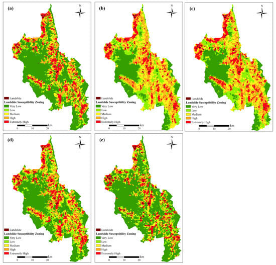
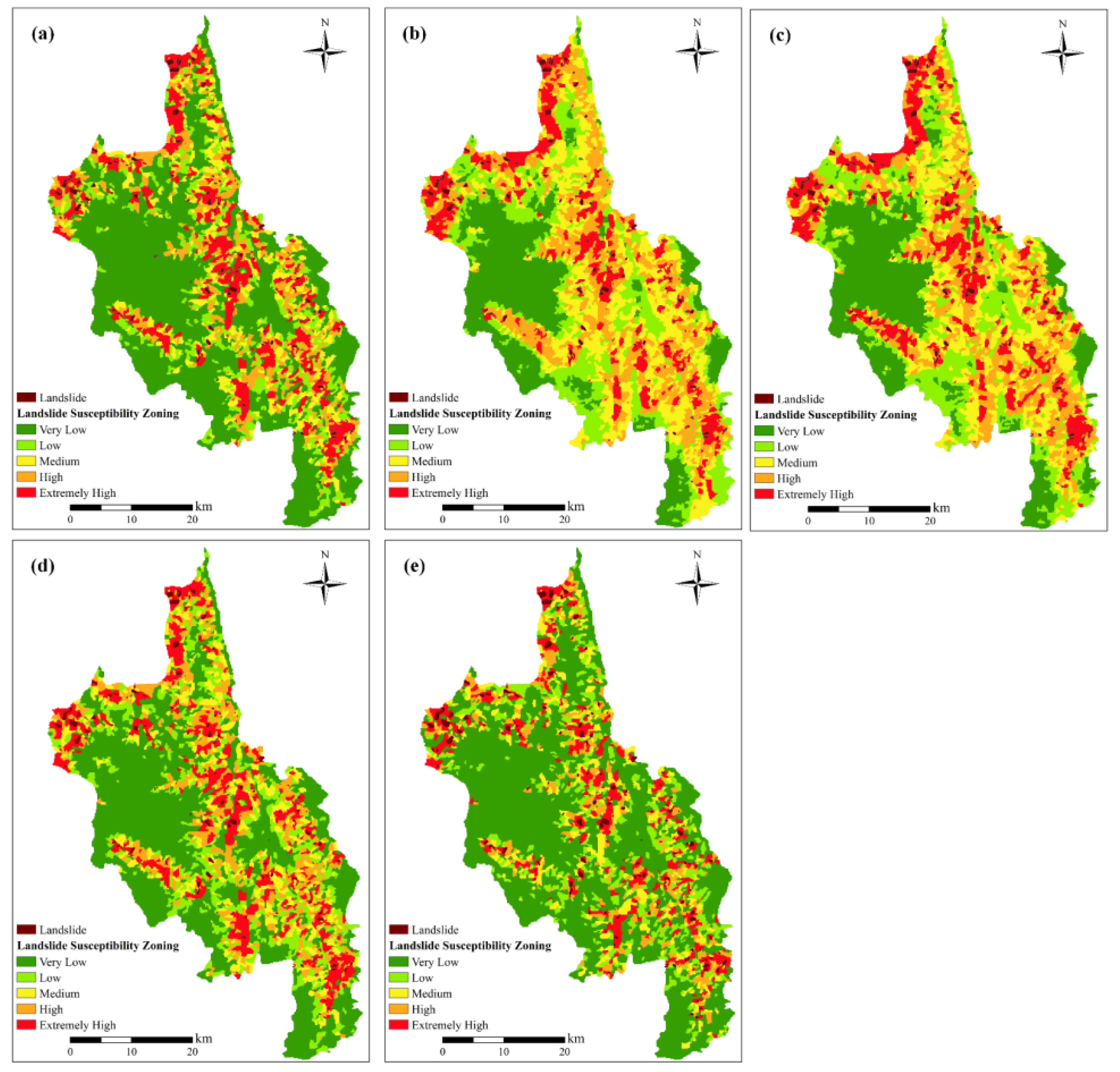
Using the TFPF-SU method to divide the slope units, the evaluation factors of the entire Dongchuan District’s slope units were input into the SVM, RF, XGBoost, and FNN landslide susceptibility models to predict the landslide susceptibility values for each slope unit. The natural breaks (Jenks) method was employed to classify the study area into five landslide susceptibility levels—very high, high, moderate, low, and very low—thereby generating the spatial distribution map of landslide susceptibility. Figure 11a–d show the landslide susceptibility classification results of the SVM, RF, XGBoost, and FNN models in Dongchuan District. In the SVM model, the proportion of slope units across five susceptibility levels, from very low to very high, is 53.19%, 13.23%, 10.82%, 9.98%, and 12.78%, respectively. In the RF model, the proportions for the five susceptibility levels from very low to very high are 23.85%, 19.63%, 21.99%, 21.56%, and 12.98%, respectively. In the XGBoost model, the proportions are 24.64%, 20.38%, 20.99%, 19.79%, and 14.20%, respectively. In the FNN model, the proportions are 46.40%, 16.77%, 12.05%, 11.37%, and 13.41%, respectively. In the AuFNN model, the proportions of very low, low, medium, high, and very high susceptibility levels are 58.43%, 13.48%, 9.35%, 7.99%, and 10.76%, respectively.
Figure 11.
Landslide geological hazard susceptibility zoning map: (a) SVM model, (b) RF model, (c) XGBoost model, (d) FNN model, (e) AuFNN model.
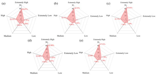
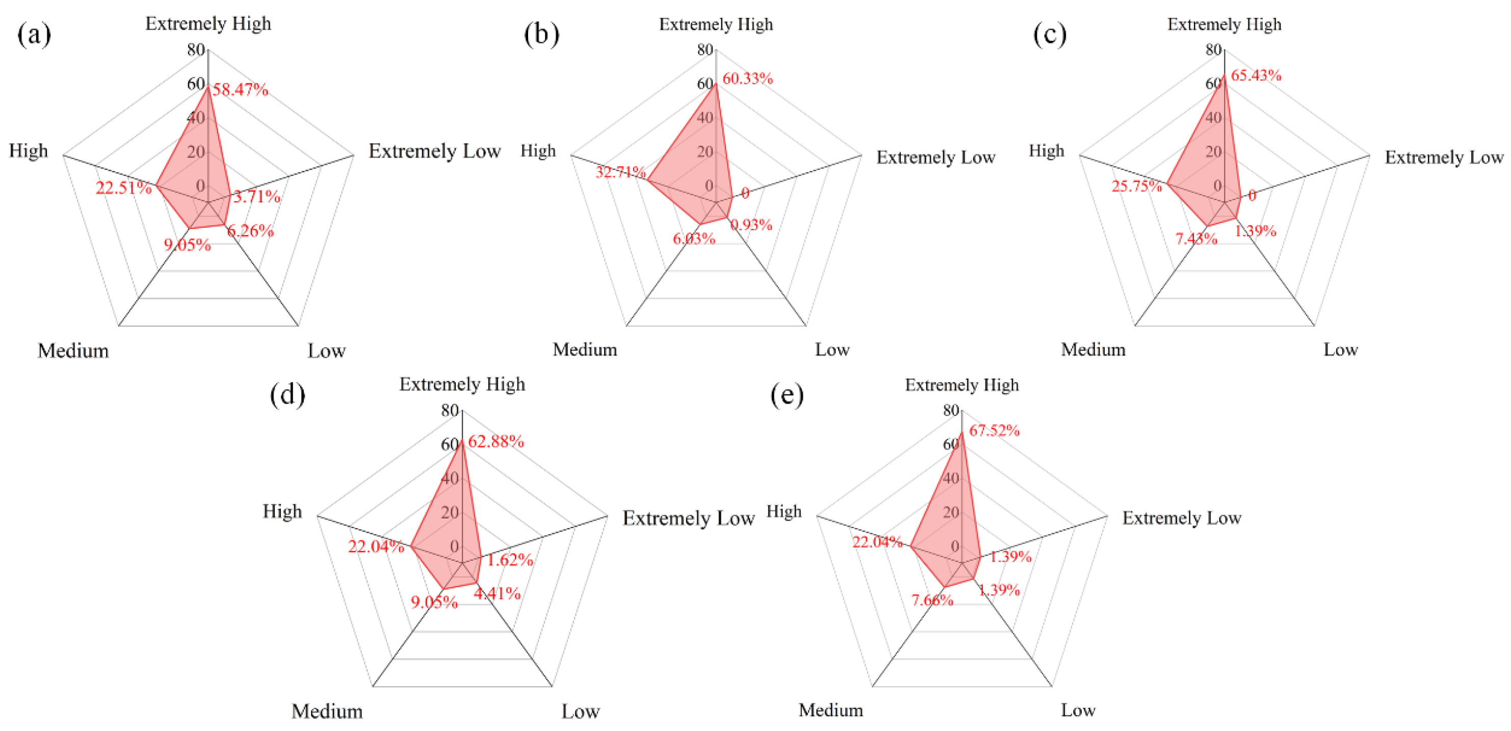
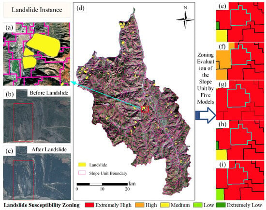
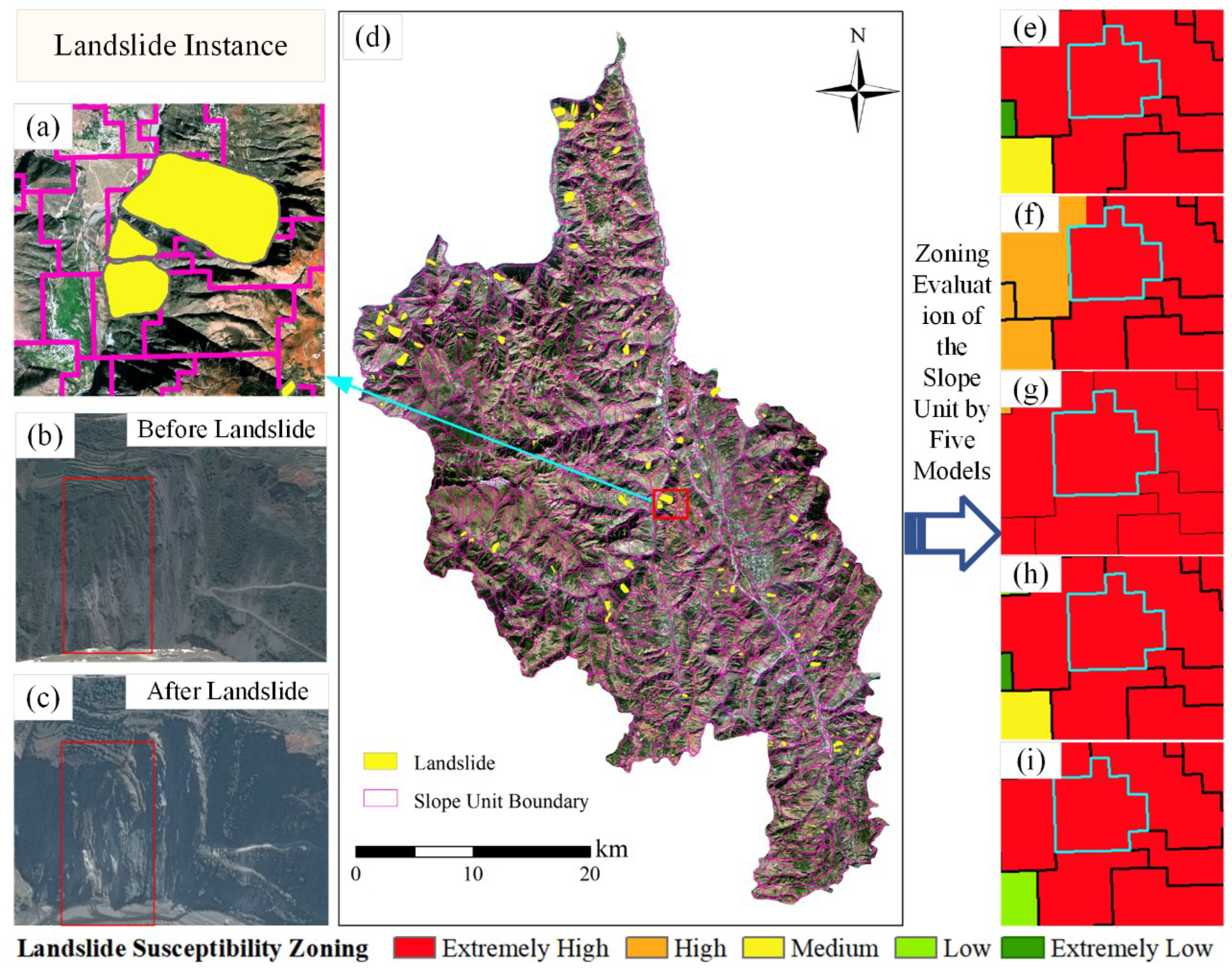
From Figure 12, it can be seen that the landslide point density is positively correlated with the landslide susceptibility zones for all four models. This result meets the rationality assessment criteria set for this study, indicating that all models perform reasonably in landslide susceptibility evaluation. Similarly, to further validate the reliability of the model predictions, the same landslide instance used earlier is applied. Under the evaluation results of all four models in this slope unit division, the landslide instance is also located in the very high susceptibility zone, as shown in Figure 13e–h, enhancing the credibility of the model predictions. Figure 13c shows the specific location of the instance, and Figure 13b,c show the comparison of remote sensing images before and after the landslide, clearly displaying the surface changes before and after the landslide event.
Figure 12.
Proportion of landslides in the susceptibility zoning: (a) SVM model, (b) RF model, (c) XGBoost model, (d) FNN model, (e) AuFNN model.
Figure 13.
(a) Enlarged view of the landslide case, (b) Pre-landslide image, (c) Post-landslide image, (d) Specific location of the landslide case, (e) Susceptibility zoning based on the SVM model, (f) Susceptibility zoning based on the RF model, (g) Susceptibility zoning based on the XGBoost model, (h) Susceptibility zoning based on the FNN model, (i) Susceptibility zoning based on the AuFNN model.
Under the evaluation results of all four models in this slope unit division, the landslide instance is also located in the very high susceptibility zone, as shown in Figure 13e–h), enhancing the credibility of the model predictions. Figure 13c shows the specific location of the instance, and Figure 13b,c show the comparison of remote sensing images before and after the landslide, clearly displaying the surface changes before and after the landslide event.
4.2. Comparison of Evaluation Results
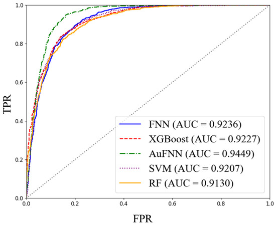
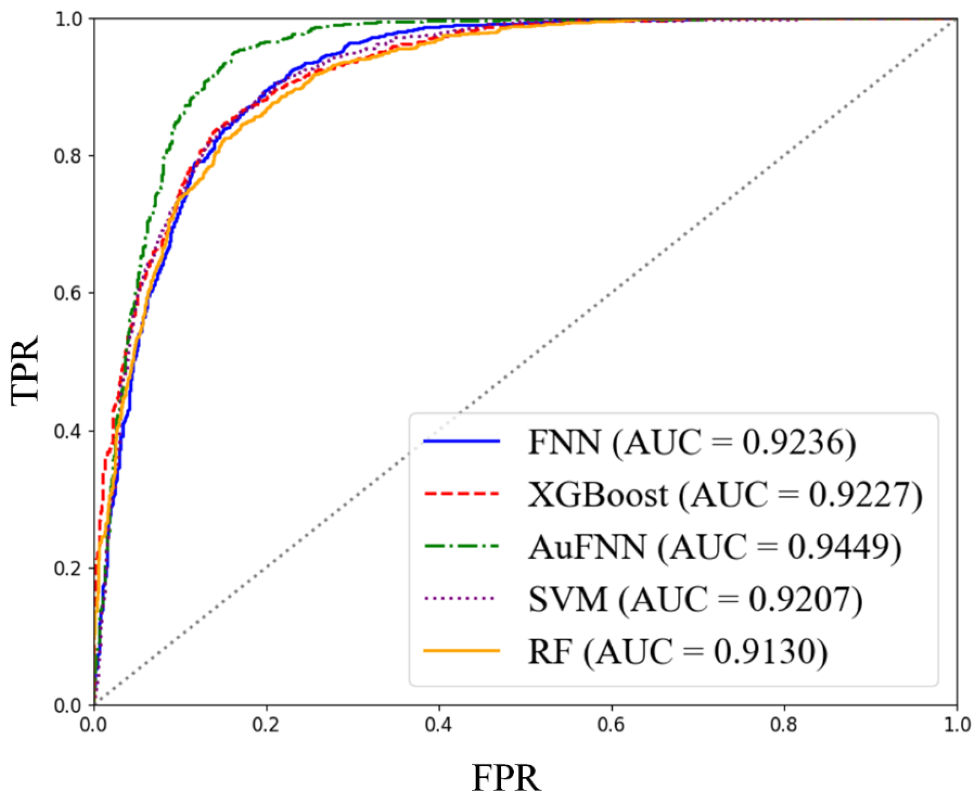
The ROC curve evaluates and quantifies the classification performance of a model by displaying the true positive rate and false positive rate at different thresholds, as well as the area under the curve (AUC value), thus providing an intuitive and comprehensive reflection of the model’s predictive capability (Figure 14). The AUC value of the AuFNN model, with slope units divided using the TFPF-SU method, is 0.9449, which is about 2% higher than SVM, 3% higher than RF, 2% higher than XGBoost, and 2% higher than FNN.
Figure 14.
ROC Curves of Different Landslide Susceptibility Assessment Models.
The results of the Accuracy, Precision, Recall, and F1 Score for the AuFNN landslide susceptibility evaluation model are shown in Table 3.
Table 3.
Evaluation Index Values of Landslide Susceptibility Models.
The results indicate that the AuFNN model (AUC = 0.9449) performs comparably to the other evaluated models, with slightly higher values observed across the evaluation metrics (FNN: 0.9236, XGBoost: 0.9227, SVM: 0.9207, and RF: 0.9130). The AuFNN model attains the highest AUC value, reflecting a marginal improvement in the overall discrimination between positive and negative samples. Overall, the AuFNN model provides a feasible and competitive approach for landslide susceptibility evaluation.
5. Discussion
This study constructs landslide susceptibility evaluation models using SVM, RF, XGBoost, FNN, and AuFNN, based on slope units delineated using the TFPF-SU method. A comparative analysis was performed using multiple evaluation metrics. The models showed good spatial consistency in the distribution of susceptibility zones, particularly in the high and very high susceptibility areas, which were concentrated in the high mountain canyon areas on both sides of the Xiaojiang River Basin. The predicted landslide susceptibility levels of the models showed a significant positive correlation with the density of known landslide points, further verifying the spatial consistency and rationality of the model predictions.
All models exhibited a higher landslide point density in the “very high” susceptibility category. The AuFNN model achieved a landslide density of 67.52% in this category, indicating that, as an alternative representation learning framework, AuFNN demonstrates performance comparable to that of established machine learning models in identifying high-susceptibility areas. The spatial distribution results suggest that the AuFNN model maintains a similar capability to existing models in distinguishing high-risk and low-risk zones, reflecting a comparable level of target specificity and reliability under the current experimental settings. These characteristics provide practical reference value for landslide disaster prevention and resource allocation, supporting the refined management of landslide-prone areas.
Different models also exhibit variations in the classification of landslide susceptibility levels. In the AuFNN model, the “very low” susceptibility level accounts for 58.43%, indicating that the model maintains stability and strong discrimination ability while avoiding overgeneralizing potential landslide areas. This demonstrates good recognition accuracy and balance. In contrast, traditional machine learning models, such as SVM and FNN, show a higher distribution proportion in the medium-to-high susceptibility areas, leading to some degree of prediction bias, which may be due to their limited ability to model high-dimensional nonlinear relationships between factors.
In terms of model performance evaluation, the AuFNN model achieved the highest values across multiple evaluation metrics, including AUC, Accuracy, Precision, Recall, and F1 Score. Notably, the AUC reached 0.9449, significantly higher than other models (SVM: 0.9207, RF: 0.9130, XGBoost: 0.9227, FNN: 0.9236), indicating superior overall performance in distinguishing between positive and negative samples. Additionally, its Recall value reached 0.9535, and the F1 Score was 0.8949, demonstrating a better balance between the completeness and accuracy of landslide sample identification. This result reflects the high applicability and potential for development of the coupled structure of autoencoder and feedforward neural network in landslide susceptibility modeling, particularly in disaster prediction tasks under complex terrain conditions.
Although the AuFNN model performed well in this study, there are still certain limitations. The selection of evaluation factors was primarily based on static terrain and surface parameters, without fully considering dynamic triggering factors such as earthquakes, which limited the model’s ability to comprehensively depict the landslide occurrence mechanisms; In this study, spatial cross-validation was not employed, and the generalization ability of the models warrants further improvement; Different categorical feature encoding strategies may influence how models represent feature information, which may in turn affect model performance. Accordingly, the results presented in this study reflect model behavior under the adopted encoding scheme; It should also be noted that while Pearson correlation analysis and the autoencoder help mitigate feature redundancy, multicollinearity is not fully addressed in a strict statistical sense. Lithology and land-use types were represented using integer encoding, which may, to some extent, influence the model learning process; therefore, the related results should be interpreted within this context.
In conclusion, the AuFNN model proposed in this study demonstrates good applicability in landslide susceptibility evaluation and provides an alternative representation learning framework with a performance comparable to that of established machine learning models. This approach offers a feasible pathway for geological hazard risk prediction under complex terrain conditions. Future research could further expand the factor system by incorporating multi-temporal dynamic data to enhance the timeliness and predictive depth of the model. In addition, validation across larger spatial extents and diverse geomorphic settings would contribute to improving its generalizability and applicability.
6. Conclusions
The accuracy of landslide susceptibility evaluation is influenced by both evaluation units and evaluation factors. In response to challenges such as feature redundancy and limitations in model representation, this study introduces an AuFNN model for landslide susceptibility evaluation and conducts comparative analysis with SVM, RF, XGBoost, and FNN using ROC curves and evaluation metrics derived from the confusion matrix. The results show that the AuFNN model achieves an AUC value of 0.9449, which is within a similar range to the results of the other models. Its Accuracy, F1 score, Precision, and Recall values are also comparable to those of the benchmark models. Overall, the AuFNN model provides an alternative representation learning framework for landslide susceptibility evaluation, demonstrating performance comparable to that of established machine learning models under the current experimental settings.
Author Contributions
Conceptualization, J.F. and K.L.; Data curation, K.L., Y.S. and P.L.; Formal analysis, K.L., Y.S. and P.L.; Funding acquisition, J.F. and Y.S.; Investigation, K.L.; Methodology, K.L. and J.F.; Project administration, J.F. and Y.S.; Resources, K.L.; Software, K.L., Y.S. and P.L.; Supervision, J.F. and Y.S.; Validation, K.L. and Y.S.; Visualization, P.L. and K.L.; Writing—original draft, K.L. and J.F.; Writing—review & editing, K.L. and J.F. All authors have read and agreed to the published version of the manuscript.
Funding
This research was funded by the National Natural Science Foundation of China (Grant No. 42171413) and a grant from the State Key Laboratory of Resources and Environmental Information System.
Institutional Review Board Statement
Not applicable.
Informed Consent Statement
Not applicable.
Data Availability Statement
The data presented in this study are available on request from the corresponding author. The data are not publicly available due to restrictions by the data collector and provider.
Acknowledgments
We sincerely thank the China Aero Geophysical Survey and Remote Sensing Center for Natural Resources for providing the data of the Dongchuan District. We also thank the editors and reviewers for their constructive comments and suggestions.
Conflicts of Interest
Author Yuqiang Sun was employed by the company CCCC Highway Consultants Co., Ltd. The remaining authors declare that the research was conducted in the absence of any commercial or financial rela-tionships that could be construed as a potential conflict of interest.
Appendix A
| Evaluation Factor | Category | Landslide Proportion | Overall Proportion | Frequency Ratio |
| Elevation (m) | 690–1216 | 0.0858 | 0.0633 | 1.3555 |
| 1216–1549 | 0.2088 | 0.124 | 1.6839 | |
| 1549–1859 | 0.232 | 0.1619 | 1.433 | |
| 1859–2186 | 0.1879 | 0.1691 | 1.1112 | |
| 2186–2538 | 0.1462 | 0.1526 | 0.9581 | |
| 2538–2924 | 0.1206 | 0.1317 | 0.9157 | |
| 2924–3376 | 0.0186 | 0.1276 | 0.1458 | |
| 3376–4116 | 0 | 0.0699 | 0 | |
| Slope (°) | 5.29–12.88 | 0.0278 | 0.0481 | 0.578 |
| 12.88–17.64 | 0.0789 | 0.1185 | 0.6658 | |
| 17.64–21.68 | 0.1137 | 0.1635 | 0.6954 | |
| 21.68–25.26 | 0.181 | 0.1712 | 1.0572 | |
| 25.26–28.85 | 0.2019 | 0.1714 | 1.1779 | |
| 28.85–32.52 | 0.2042 | 0.1478 | 1.3816 | |
| 32.52–36.63 | 0.1369 | 0.118 | 1.1602 | |
| 36.63–49.2 | 0.0557 | 0.0615 | 0.9057 | |
| Plan Curvature | −1.39–0.15 | 0.0139 | 0.0211 | 0.6588 |
| −0.15–0.08 | 0.051 | 0.0581 | 0.8778 | |
| −0.08–0.03 | 0.1647 | 0.1557 | 1.0578 | |
| −0.03–0 | 0.232 | 0.2023 | 1.1468 | |
| 0–0.03 | 0.1926 | 0.2293 | 0.8399 | |
| 0.03–0.07 | 0.2251 | 0.1868 | 1.205 | |
| 0.07–0.13 | 0.0789 | 0.1024 | 0.7705 | |
| 0.13–0.46 | 0.0418 | 0.044 | 0.95 | |
| Profile Curvature | −0.56–0.19 | 0.0116 | 0.0202 | 0.5743 |
| −0.19–0.09 | 0.1021 | 0.1162 | 0.8787 | |
| −0.09–0.03 | 0.1694 | 0.1893 | 0.8949 | |
| −0.03–0 | 0.1346 | 0.1512 | 0.8902 | |
| 0–0.05 | 0.2529 | 0.2468 | 1.0247 | |
| 0.05–0.1 | 0.1787 | 0.1464 | 1.2206 | |
| 0.1–0.19 | 0.1346 | 0.0967 | 1.3919 | |
| 0.19–1.61 | 0.0162 | 0.0329 | 0.4924 | |
| NDVI | −0.43–0.12 | 0.0093 | 0.0107 | 0.8692 |
| −0.12–0 | 0.123 | 0.0774 | 1.5891 | |
| 0–0.07 | 0.2088 | 0.1725 | 1.2104 | |
| 0.07–0.13 | 0.1879 | 0.2132 | 0.8813 | |
| 0.13–0.19 | 0.2042 | 0.2198 | 0.929 | |
| 0.19–0.26 | 0.1671 | 0.173 | 0.9659 | |
| 0.26–0.35 | 0.0812 | 0.0926 | 0.8769 | |
| 0.35–0.53 | 0.0186 | 0.0406 | 0.4581 | |
| TWI | 4.51–5.38 | 0.1555 | 0.1882 | 0.8262 |
| 5.38–5.71 | 0.2923 | 0.2613 | 1.1186 | |
| 5.71–6.06 | 0.2691 | 0.2597 | 1.0362 | |
| 6.06–6.53 | 0.1439 | 0.1662 | 0.8658 | |
| 6.53–7.34 | 0.0835 | 0.0804 | 1.0386 | |
| 7.34–9.13 | 0.0441 | 0.032 | 1.3781 | |
| 9.13–11.97 | 0.0116 | 0.0084 | 1.381 | |
| 11.97–16.42 | 0 | 0.0039 | 0 | |
| Annual Precipitation (mm) | 766–779 | 0.051 | 0.0779 | 0.6547 |
| 779–785 | 0.0974 | 0.1012 | 0.9625 | |
| 785–791 | 0.2181 | 0.1739 | 1.2542 | |
| 791–796 | 0.2019 | 0.1891 | 1.0677 | |
| 796–802 | 0.2065 | 0.1871 | 1.1037 | |
| 802–808 | 0.116 | 0.1512 | 0.7672 | |
| 808–817 | 0.0766 | 0.0922 | 0.8308 | |
| 817–834 | 0.0325 | 0.0275 | 1.1818 | |
| Land Use | Cultivated Land | 0.288 | 0.244 | 1.18 |
| Grassland | 0.603 | 0.638 | 0.945 | |
| Forest Land | 0.09 | 0.107 | 0.841 | |
| Artificial Surface | 0.019 | 0.011 | 1.727 | |
| Water Body | 0 | 0 | 0 | |
| Aspect | Southwest | 0.2274 | 0.1827 | 1.2447 |
| South | 0.1346 | 0.1921 | 0.7007 | |
| Southeast | 0.1787 | 0.254 | 0.7035 | |
| East | 0.1485 | 0.173 | 0.8584 | |
| Northeast | 0.0209 | 0.0179 | 1.1676 | |
| West | 0.2599 | 0.1569 | 1.6565 | |
| Northwest | 0.0278 | 0.0218 | 1.2752 | |
| North | 0.0023 | 0.0016 | 1.4375 | |
| Flat | 0 | 0 | 0 | |
| Lithology | Extremely Weak Rock Formation | 0.049 | 0.069 | 0.71 |
| Moderately Soft to Moderately Hard Rock | 0.005 | 0.003 | 1.667 | |
| Moderately Hard to Hard Rock | 0.237 | 0.355 | 0.668 | |
| Moderately Hard Rock Formation | 0.501 | 0.436 | 1.149 | |
| Hard Rock Formation | 0.021 | 0.019 | 1.105 | |
| Moderately Weak Rock Formation | 0.167 | 0.101 | 1.653 | |
| Moderately Hard Rock Formation with Weak Interlayers | 0.005 | 0.005 | 1 | |
| Weak Rock Formation | 0.016 | 0.012 | 1.333 | |
| Hard Rock Formation with Weak Interlayers | 0 | 0 | 0 | |
| Distance to Fault (m) | 0–200 | 0.176 | 0.147 | 1.197 |
| 200–400 | 0.204 | 0.191 | 1.068 | |
| 400–600 | 0.135 | 0.127 | 1.063 | |
| 600–800 | 0.088 | 0.098 | 0.898 | |
| 800–1000 | 0.077 | 0.077 | 1 | |
| 1000–1200 | 0.065 | 0.058 | 1.121 | |
| 1200–1400 | 0.049 | 0.047 | 1.043 | |
| >1400 | 0.206 | 0.255 | 0.808 | |
| Distance to River (m) | 0–200 | 0.06 | 0.038 | 1.579 |
| 200–400 | 0.095 | 0.074 | 1.284 | |
| 400–600 | 0.093 | 0.046 | 2.022 | |
| 600–800 | 0.074 | 0.051 | 1.451 | |
| 800–1000 | 0.07 | 0.044 | 1.591 | |
| 1000–1200 | 0.053 | 0.045 | 1.178 | |
| 1200–1400 | 0.056 | 0.051 | 1.098 | |
| >1400 | 0.499 | 0.651 | 0.767 | |
| Distance to Road (m) | 0–200 | 0.283 | 0.24 | 1.179 |
| 200–400 | 0.232 | 0.159 | 1.459 | |
| 400–600 | 0.132 | 0.095 | 1.389 | |
| 600–800 | 0.086 | 0.065 | 1.323 | |
| 800–1000 | 0.072 | 0.05 | 1.44 | |
| 1000–1200 | 0.032 | 0.04 | 0.8 | |
| 1200–1400 | 0.053 | 0.039 | 1.359 | |
| >1400 | 0.109 | 0.312 | 0.349 |
References
- Ado, M.; Amitab, K.; Maji, A.K.; Jasinska, E.; Gono, R.; Leonowicz, Z.; Jasinski, M. Landslide Susceptibility Mapping Using Machine Learning: A Literature Survey. Remote Sens. 2022, 14, 3029. [Google Scholar] [CrossRef] [Scilit]
- Reichenbach, P.; Rossi, M.; Malamud, B.D.; Mihir, M.; Guzzetti, F. A review of statistically-based landslide susceptibility models. Earth-Sci. Rev. 2018, 180, 60–91. [Google Scholar] [CrossRef] [Scilit]
- Huang, F.M.; Xiong, H.W.; Jiang, S.H.; Yao, C.; Fan, X.M.; Catani, F.; Chang, Z.L.; Zhou, X.T.; Huang, J.S.; Liu, K.J. Modelling landslide susceptibility prediction: A review and construction of semi-supervised imbalanced theory. Earth-Sci. Rev. 2024, 250, 104700. [Google Scholar] [CrossRef] [Scilit]
- Huang, F.M.; Xiong, H.W.; Yao, C.; Catani, F.; Zhou, C.B.; Huang, J.S. Uncertainties of landslide susceptibility prediction considering different landslide types. J. Rock Mech. Geotech. Eng. 2023, 15, 2954–2972. [Google Scholar] [CrossRef] [Scilit]
- Sun, D.L.; Gu, Q.Y.; Wen, H.J.; Xu, J.H.; Zhang, Y.L.; Shi, S.X.; Xue, M.M.; Zhou, X.Z. Assessment of landslide susceptibility along mountain highways based on different machine learning algorithms and mapping units by hybrid factors screening and sample optimization. Gondwana Res. 2023, 123, 89–106. [Google Scholar] [CrossRef] [Scilit]
- Sun, D.L.; Wu, X.Q.; Wen, H.J.; Gu, Q.Y. A LightGBM-based landslide susceptibility model considering the uncertainty of non-landslide samples. Geomat. Nat. Hazards Risk 2023, 14, 2213807. [Google Scholar] [CrossRef] [Scilit]
- Guo, F.; Lai, P.; Huang, F.; Liu, L.; Wang, X.; He, Z. A Literature Review and Research Progress on Landslide Susceptibility Assessment Based on Knowledge Graphs. Earth Sci.-J. China Univ. Geosci. 2024, 49, 1584–1606. [Google Scholar] [CrossRef] [Scilit]
- Miller, R.D.; Dobrovolny, E. Surficial Geology of Anchorage and Vicinity, Alaska; US Government Printing Office: Washington, DC, USA, 1959; Volume 1093.
- Huang, W.B.; Ding, M.T.; Li, Z.H.; Yu, J.C.; Ge, D.Q.; Liu, Q.; Yang, J. Landslide susceptibility mapping and dynamic response along the Sichuan-Tibet transportation corridor using deep learning algorithms. Catena 2023, 222, 106866. [Google Scholar] [CrossRef] [Scilit]
- Nanehkaran, Y.A.; Chen, B.Y.; Cemiloglu, A.; Chen, J.D.; Anwar, S.; Azarafza, M.; Derakhshani, R. Riverside Landslide Susceptibility Overview: Leveraging Artificial Neural Networks and Machine Learning in Accordance with the United Nations (UN) Sustainable Development Goals. Water 2023, 15, 2707. [Google Scholar] [CrossRef] [Scilit]
- Dias, H.C.; Hölbling, D.; Grohmann, C.H. Landslide Susceptibility Mapping in Brazil: A Review. Geosciences 2021, 11, 425. [Google Scholar] [CrossRef] [Scilit]
- Carrara, A.; Cardinali, M.; Guzzetti, F.; Reichenbach, P. GIS Technology in Mapping Landslide Hazard. Geomorphology 1995, 11, 103–118. [Google Scholar]
- Saaty, T.L. A Scaling Method for Priorities in Hierarchical Structures. J. Math. Psychol. 1977, 15, 234–281. [Google Scholar] [CrossRef] [Scilit]
- Ayalew, L.; Yamagishi, H. The Application of GIS-Based Logistic Regression for Landslide Susceptibility Mapping in the Kakuda–Yahiko Mountains, Central Japan. Geomorphology 2005, 65, 15–31. [Google Scholar] [CrossRef] [Scilit]
- Moragues, S.; Lenzano, M.G.; Lanfri, M.; Moreiras, S.; Lannutti, E.; Lenzano, L. Analytic hierarchy process applied to landslide susceptibility mapping of the North Branch of Argentino Lake, Argentina. Nat. Hazards 2021, 105, 915–941. [Google Scholar] [CrossRef] [Scilit]
- Baharvand, S.; Rahnamarad, J.; Soori, S.; Saadatkhah, N. Landslide susceptibility zoning in a catchment of Zagros Mountains using fuzzy logic and GIS. Environ. Earth Sci. 2020, 79. [Google Scholar] [CrossRef] [Scilit]
- Ali, S.A.; Parvin, F.; Vojteková, J.; Costache, R.; Linh, N.T.T.; Pham, Q.B.; Vojtek, M.; Gigovic, L.; Ahmad, A.; Ghorbani, M.A. GIS-based landslide susceptibility modeling: A comparison between fuzzy multi-criteria and machine learning algorithms. Geosci. Front. 2021, 12, 857–876. [Google Scholar] [CrossRef] [Scilit]
- Achu, A.L.; Thomas, J.; Aju, C.D.; Vijith, H.; Gopinath, G. Redefining landslide susceptibility under extreme rainfall events using deep learning. Geomorphology 2024, 448, 109033. [Google Scholar] [CrossRef] [Scilit]
- Huang, Y.; Zhao, L. Review on landslide susceptibility mapping using support vector machines. Catena 2018, 165, 520–529. [Google Scholar] [CrossRef] [Scilit]
- Guo, Y.; Dou, J.; Xiang, Z.; Ma, H.; Dong, A.; Luo, W. Wenchuan Co-Seismic Landslide Susceptibility Assessment Using Gradient Boosting Decision Trees and Random Forests Based on an Optimized Negative Sample Sampling Strategy. Geosci. Technol. Bull. 2024, 43, 251–265. [Google Scholar] [CrossRef]
- Peng, S.; Liu, P.; Chen, G.; Wang, L.; Zhang, W.; Luo, W.; Jing, X. Regional Landslide Hazard Assessment and Zoning Based on the Coupled Information Value Method and Random Forest Model with Critical Monthly Average Rainfall Threshold: A Case Study of Fuling District, Chongqing. J. Geol. Hazards Prev. 2025, 36, 131–145. [Google Scholar] [CrossRef]
- Zhang, W.; He, Y.; Wang, L.; Liu, S.; Meng, X. Landslide Susceptibility mapping using random forest and extreme gradient boosting: A case study of Fengjie, Chongqing. Geol. J. 2023, 58, 2372–2387. [Google Scholar] [CrossRef] [Scilit]
- Nikoobakht, S.; Azarafza, M.; Akgün, H.; Derakhshani, R. Landslide Susceptibility Assessment by Using Convolutional Neural Network. Appl. Sci. 2022, 12, 5992. [Google Scholar] [CrossRef] [Scilit]
- Chang, Z.; Huang, F.; Jiang, S.; Zhang, Y.; Zhou, C.; Huang, J. Slope Unit Delineation and Landslide Susceptibility Prediction Based on a Multi-Scale Segmentation Method. Eng. Sci. Technol. 2023, 55, 184–195. [Google Scholar] [CrossRef]
- Moayedi, H.; Mehrabi, M.; Mosallanezhad, M.; Rashid, A.S.A.; Pradhan, B. Modification of landslide susceptibility mapping using optimized PSO-ANN technique. Eng. Comput. 2019, 35, 967–984. [Google Scholar] [CrossRef] [Scilit]
- Sharma, N.; Saharia, M.; Ramana, G.V. High resolution landslide susceptibility mapping using ensemble machine learning and geospatial big data. Catena 2024, 235, 107653. [Google Scholar] [CrossRef] [Scilit]
- Dou, J.; Xiang, Z.; Xu, Q.; Zheng, P.; Wang, X.; Su, A.; Liu, J.; Luo, W. Applications and Development Trends of Machine Learning in Intelligent Landslide Disaster Prevention and Mitigation. Earth Sci.-J. China Univ. Geosci. 2023, 48, 1657–1674. [Google Scholar] [CrossRef] [Scilit]
- Wang, S.; Wang, R.; Sun, X.; Liu, X.; Lu, W.; Lin, Z.A. Landslide Susceptibility Assessment Based on a CF-CNN-LSTM Model. J. Nat. Disasters 2024, 33, 84–95. [Google Scholar] [CrossRef]
- Zeng, T.; Wu, L.; Peduto, D.; Glade, T.; Hayakawa, Y.S.; Yin, K. Ensemble learning framework for landslide susceptibility mapping: Different basic classifier and ensemble strategy. Geosci. Front. 2023, 14, 101645. [Google Scholar] [CrossRef] [Scilit]
- Yu, L.; Wang, Y.; Pradhan, B. Enhancing landslide susceptibility mapping incorporating landslide typology via stacking ensemble machine learning in Three Gorges Reservoir, China. Geosci. Front. 2024, 15, 101802. [Google Scholar] [CrossRef] [Scilit]
- Li, P.; Fan, J.F.; Du, Y.J.; Li, K.; Zhou, Y.K. A New Parameter-Free Slope Unit Division Method That Integrates Terrain Factors. Appl. Sci. 2024, 14, 11279. [Google Scholar] [CrossRef] [Scilit]
- Arabameri, A.; Pradhan, B.; Rezaei, K.; Lee, C.-W. Assessment of Landslide Susceptibility Using Statistical- and Artificial Intelligence-Based FR–RF Integrated Model and Multiresolution DEMs. Remote Sens. 2019, 11, 999. [Google Scholar] [CrossRef] [Scilit]
- Guzzetti, F.; Carrara, A.; Cardinali, M.; Reichenbach, P. Landslide hazard evaluation: A review of current techniques and their application in a multi-scale study, Central Italy. Geomorphology 1999, 31, 181–216. [Google Scholar] [CrossRef] [Scilit]
- Cruden, D.M.; Varnes, D.J. Landslide types and processes. In Landslides: Investigation and Mitigation; Turner, A.K., Schuster, R.L., Eds.; Transportation Research Board, National Research Council: Washington, DC, USA, 1996; pp. 36–75. [Google Scholar]
- Li, Y.; Xu, Q.; Zhang, B.; Fan, X.; Huang, R. Spatial Distribution of Near-Fault Landslides along the Litang Fault Zone, Eastern Tibetan Plateau. Geomorphology 2024, 455, 109189. [Google Scholar] [CrossRef] [Scilit]
- Zhang, Y.; Xu, C.; Shao, X.; Li, H. Dependence of Coseismic Landslide Distribution Patterns on Fault Movement. Appl. Sci. 2025, 15, 10305. [Google Scholar] [CrossRef] [Scilit]
- Yan, W.; Guo, T.; Yang, Y.; Hua, Y.; Zhou, X.; Zhang, Z. Regional Landslide Sensitivity Analysis Based on the WOE-PPMCC Model. Geol. Sci. 2024, 59, 1775–1785. [Google Scholar]
- Qiu, H.; Cao, M.; Liu, W.; Wang, Y.; Hao, J.; Hu, S. Regional Landslide Susceptibility Assessment and Result Validation Based on Three Different Models. Geogr. Sci. 2014, 34, 110–115. [Google Scholar] [CrossRef]
- Guo, Z. Landslide Susceptibility Assessment Based on GIS and WOE-BP Model. Earth Sci.-J. China Univ. Geosci. 2019, 44, 4299–4312. [Google Scholar] [CrossRef] [Scilit]
- Li, W.; Fan, X.; Huang, F.; Wu, X.; Yin, K.; Chang, Z. Landslide Susceptibility Modeling Uncertainty under Different Combinations of Environmental Factors and Prediction Models. Earth Sci.-J. China Univ. Geosci. 2021, 46, 3777–3795. [Google Scholar] [CrossRef] [Scilit]
- Mustafa Abdullah, D.; Mohsin Abdulazeez, A. Machine Learning Applications based on SVM Classification A Review. Qubahan Acad. J. 2021, 1, 81–90. [Google Scholar] [CrossRef] [Scilit]
- Yang, L.; Wei, J.; Xu, Z. Landslide Displacement Prediction Based on Smooth Prior Method–Sparrow Search Algorithm–Support Vector Machine Regression Model: A Case Study of Bazimen and Baishuihe Landslides in the Three Gorges Reservoir Area. J. Earth Sci. Environ. 2022, 44, 1096–1110. [Google Scholar] [CrossRef]
- Li, C.; Liu, Y.; Lai, S.; Wang, D.; He, X.; Liu, Q. Landslide Susceptibility Analysis Based on a Coupled Logistic Regression and Support Vector Machine Model. J. Nat. Disasters 2024, 33, 75–86. [Google Scholar] [CrossRef]
- Breiman, L. Random forests. Mach. Learn. 2001, 45, 5–32. [Google Scholar] [CrossRef] [Scilit]
- Zhang, X.; Su, Q.; Zhao, C.; Zhu, Y.; Li, K.; Fan, J.; Bai, D. A Landslide Susceptibility Assessment Method Based on XGBoost Optimized by Bayesian Algorithm. J. Geomat. Sci. 2023, 48, 140–150. [Google Scholar] [CrossRef]
- Chen, T.; Guestrin, C. Xgboost: A scalable tree boosting system. In Proceedings of the 22nd ACM SIGKDD International Conference on Knowledge Discovery and Data Mining, San Francisco, CA, USA, 13–17 August 2016; pp. 785–794. [Google Scholar]
- Bebis, G.; Georgiopoulos, M. Feed-forward neural networks. IEEE Potentials 1994, 13, 27–31. [Google Scholar] [CrossRef] [Scilit]
- Wang, J.; Zang, M.; Xu, C.; Liu, T.; Huang, Y. 2022 Luding Earthquake Landslide Susceptibility Assessment Based on a Coupled Algorithm of Analytic Hierarchy Process and Area Under the Receiver Operating Characteristic Curve. Chin. J. Eng. Geol. 2024, 32, 1696–1711. [Google Scholar] [CrossRef]
- Ai, X.; Zhang, J.; Fu, J. Analysis of Differences in Regional Earthquake-Induced Landslide Hazard Predictions Using Different Feature Selection Methods: A Case Study of the Wenchuan Earthquake Area. S. China Earthq. 2024, 44, 39–51. [Google Scholar] [CrossRef]
- Chen, Z. Research on a Geological Hazard Susceptibility Assessment Model and Its Application Based on Ensemble Machine Learning. Master’s Thesis, Lanzhou University of Technology, Lanzhou, China, 2023. [Google Scholar]
- Liu, R.; Shi, W.; Sun, D.; Xu, J. Landslide Susceptibility Zoning of Wushan County Based on GIS and Random Forest. J. Chongqing Norm. Univ. (Nat. Sci. Ed.) 2020, 37, 86–96. [Google Scholar]

Disclaimer/Publisher’s Note: The statements, opinions and data contained in all publications are solely those of the individual author(s) and contributor(s) and not of MDPI and/or the editor(s). MDPI and/or the editor(s) disclaim responsibility for any injury to people or property resulting from any ideas, methods, instructions or products referred to in the content. |
© 2026 by the authors. Licensee MDPI, Basel, Switzerland. This article is an open access article distributed under the terms and conditions of the Creative Commons Attribution (CC BY) license.