Machine Learning and Deep Learning Techniques for Fault Location in Transmission Lines

Abstract

Fault location in a power system is a sensitive task because of the grid’s complex environment. Traditional fault-location methods that rely only on impedance estimates or traveling waves are less accurate than before because modern transmission networks are more complex due to the integration of wind resources, power electronic interfaces, and changing operating conditions. This study provides an artificial intelligence-based comparative framework for transmission line fault locating based on models such as artificial neural network (ANN), adaptive neuro-fuzzy inference system (ANFIS), convolutional neural network (CNN), long short-term memory network (LSTM), and bidirectional long short-term memory network (BiLSTM). The suggested configuration is tested on both the IEEE 9-bus test system and the IEEE 30-bus test system to explore the impact of the size and complexity of the network on model performance. The test systems are simulated in MATLAB (Version R2024a)/Simulink for various operating conditions, fault locations, and fault types. The faults are measured by three-phase voltage and three-phase current at one end of the transmission line, and the distance to the fault is used as the regression variable for the modeling. The mean square error, root mean square error, mean absolute error, coefficient of determination, as well as training and testing performance in modifying the models, are used for assessing model performance. ANFIS has yielded the best results for the verified fault location of the IEEE 9-bus system, with RMSE, MAE, and R² equal to 1.880 km, 1.142 km, and 0.996, respectively, and better than the traditional ANN model and other deep learning models. The deep learning technique that performed best on the larger system, the 30-bus IEEE system, was BiLSTM with a testing RMSE of 2.909 km, an MAE of 1.841 km, and an R² value of 0.998. The results showed that ANFIS shows good performance in the small category of the system due to its nonlinear rule-based learning, while, on the other hand, BiLSTM has good performance in larger-scale and complex systems owing to its learning capability in a bidirectional manner in voltage and current signals. The comparative analysis presented in this work reveals that intelligent regression models can estimate single-ended fault location, are robust, and have great potential for use in real-time transmission line protection systems.

1. Introduction

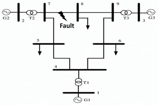
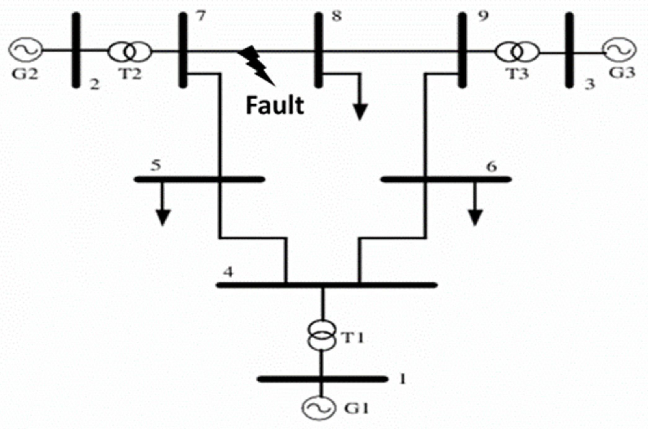
The stability of modern power systems depends more on the reliable performance of transmission lines, which form the backbone of electrical power systems. Due to the penetration of renewable energy sources and power electronic devices, the complexity of the transmission system has increased significantly [1,2]. As a result, transmission line faults pose a serious threat to the system’s reliability, continuity of power supply, and security of the power system. Accurate fault detection and location are, therefore, important to minimize system damage, reduce outage duration, and improve system protection and its performance. In such a complex environment, fault detection and location in transmission lines have become an important research area to explore for both researchers and control engineers. Traditional protection systems in power systems depend more on relays, phasor measurement units, and circuit breakers for fault detection and isolation. These methods are used worldwide. However, their performance is often limited under complex conditions, especially in systems with renewable integration, distributed generation, and other nonlinear situations [3]. The changing nature of power systems today demands more flexible and smarter fault detection and location tools. In this regard, machine learning and deep learning may also offer a way to manage complex nonlinear connections, identify non-obvious features, and enhance fault classification and location accuracy [4,5]. These models exhibit great potential in addressing challenges such as fault location in diverse operating scenarios [6]. They can effectively learn the behavior and automatically generate discriminative features, making them ideal for fault detection and location of transmission lines [7,8]. This paper presents comparative results of methods that use machine learning and deep learning architectures incorporating artificial neural networks (ANN), adaptive neural fuzzy inference system (ANFIS), convolutional neural networks (CNN), long short-term memory (LSTM), and bidirectional long short-term memory (BiLSTM). The approach uses single-end measurements, eliminating the requirement for multi-end coordinated exchange of measurements and thus communication complexity [9]. Discrete wavelet transform (DWT) is introduced for capturing transients post-fault to detect faults in large systems such as the IEEE 9-bus system and IEEE 30-bus system. DWT has gained significant attention as being simple, accurate, and effective for capturing transients in balanced as well as unbalanced fault cases [10]. Various wavelet-based fault location methods have been proposed. For instance, wavelet transform-based fault location approaches with GPS synchronization [11] are highly accurate, but their performance may be affected by weak or lost GPS signals. The use of hybrid deep learning has also been extensively explored. A CNN and BiLSTM attention approach was proposed in [12] to deal with the complexity of distribution systems with high distributed generation. This model can extract spatial and complex features from zero-sequence current signals and is insensitive to various fault types. While it has strong feature extraction and learning ability, it involves attention-based mechanisms, which make it a more complex method and unsuitable for real-time applications. Furthermore, the proposed model is primarily designed for single-phase grounding faults, and it should be evaluated for other asymmetrical faults. Another approach is to use traveling-wave-based algorithms. Adaptive waveform similarity techniques have also been applied to enhance fault location in complex systems through waveform matching [13]. Likewise, novel traveling wave methods involving successive variational mode decomposition and wave velocity with frequency-dependent parameters have demonstrated good performance [14]. But such approaches often require significant signal preprocessing, iterative algorithms, and matrix calculations, leading to higher computational complexity and potentially limiting their applicability to the real-time environment. In addition, single-ended traveling wave techniques combined with DWT and support vector machines (SVM) have shown good performance in hybrid transmission lines [15]. Although the DWT efficiently captures transient features, support vector machine (SVM) based approaches are sensitive to changes in system topology and operating conditions. The problem of fault location has been widely investigated, but still has limitations. While many machine learning and deep learning methods are capable of delivering high fault location accuracy, it is generally at the cost of high computational complexity, and some of the wavelet- and traveling wave-based methods demand complicated signal preprocessing or require critical time ambiguities. Moreover, many existing models do not have good generalization capability under some unbalanced fault scenarios. Hence, a highly accurate and low-computation-complexity fault location approach that can effectively integrate features with the capability to cover diverse fault conditions is highly desired. Besides, most of the existing approaches are either based on the waveform or features from a single domain, without using the transient features of wavelets and engineered features of the electrical nature, under global learning scenarios. In this regard, this paper proposes integrating DWT-based machine learning and deep learning approaches such as ANN, ANFIS, CNN, LSTM, and BiLSTM to facilitate effective and efficient fault location schemes (Figure 1). DWT captures characteristics such as high-frequency components and signal discontinuities of faults, and these features are key to fault detection [16].

Figure 1. IEEE 9-bus system [17,18].

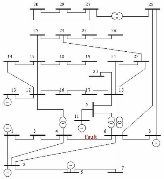
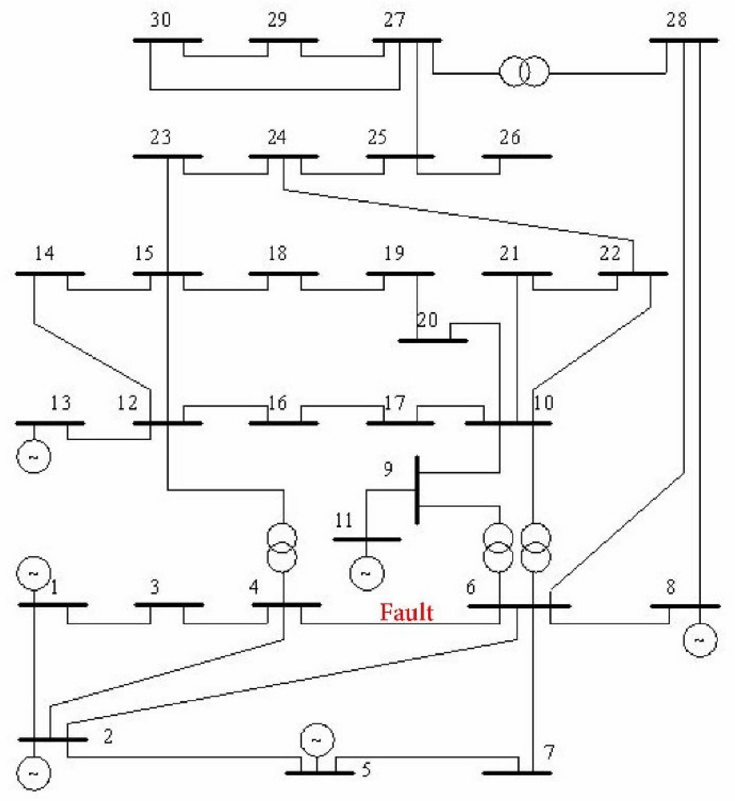
Machine learning techniques perform well in specific tasks using voltage and current. ANN and ANFIS are good at locating the exact location of a fault in a transmission line and classifying it. There are techniques that integrate ANN and ANFIS with the Global Positioning System (GPS) for locating faults [19]. Therefore, the use of ANN and ANFIS independently using post-fault voltage and current could produce better results. Among deep learning techniques, CNN learns spatial dependencies from the voltage, current, and wavelet representations, facilitating a hierarchical representation of fault-related features [20]. Fault signals are dynamic in nature, and, therefore, LSTM and BiLSTM are applied to capture relationships in fault signals [17]. BiLSTM’s bidirectional approach also shows improved results by learning from both past and future inputs. The proposed approach in this work is different from that employed in existing literature; it merges features from DWT and the post-fault voltage and current from two test systems for developing models for training and testing and comparing the various machine learning and deep learning models. All operate under identical conditions for systematic assessment of ANN, ANFIS, CNN, LSTM, and BiLSTM models for single-ended fault location of transmission lines. The proposed DWT-based ANN, ANFIS, CNN, LSTM, and BiLSTM approaches are thus likely to deliver efficient, robust, and reliable fault location under varying fault conditions. The novelty in this research is the development of a single, integrated, and feature-based fault location framework that incorporates the wavelet features of transients along with three-phase voltage and current signals. This work extends beyond prior methods that largely depend on a raw waveform input or single-domain feature space by introducing a novel feature-level multi-domain fusion approach to enhance location sensitivity and feature separability. Moreover, the performance of ANN, ANFIS, CNN, LSTM, and BiLSTM is compared under the same preprocessing, model training, and testing conditions, providing an equal platform for analysis. This allows evaluation of the trade-offs between model complexity, feature learning, and fault location results under a single-ended fault location scenario. There are three main contributions in this work: first, a feature fusion framework was designed to mix measured electrical parameters, the transient information derived from DWT analysis, and physically meaningful parameters in a single input representation for the purpose of fault location for a single-ended transmission line. This allows the learning models to use steady-state electrical and transient fault information, not a single domain of features. Second, ANN, ANFIS, CNN, LSTM, and BiLSTM are evaluated using the same input features and consistent training and testing, allowing the influence of learning architecture to be examined without confounding differences in feature construction or dataset preparation. Third, the framework is deployed on both IEEE 9-bus and IEEE 30-bus systems under multiple fault locations and fault conditions to evaluate its applicability for different network configurations (Figure 2).

Figure 2. IEEE 30-bus system [21,22].

2. System and Fault Localization Techniques

2.1. System and Fault Simulation

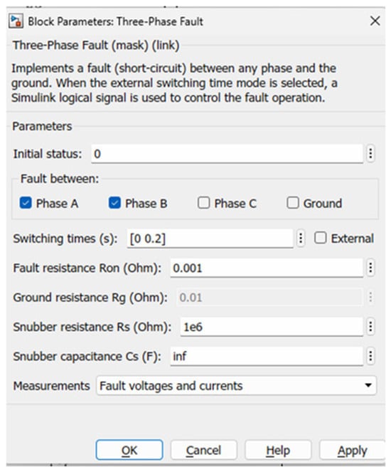
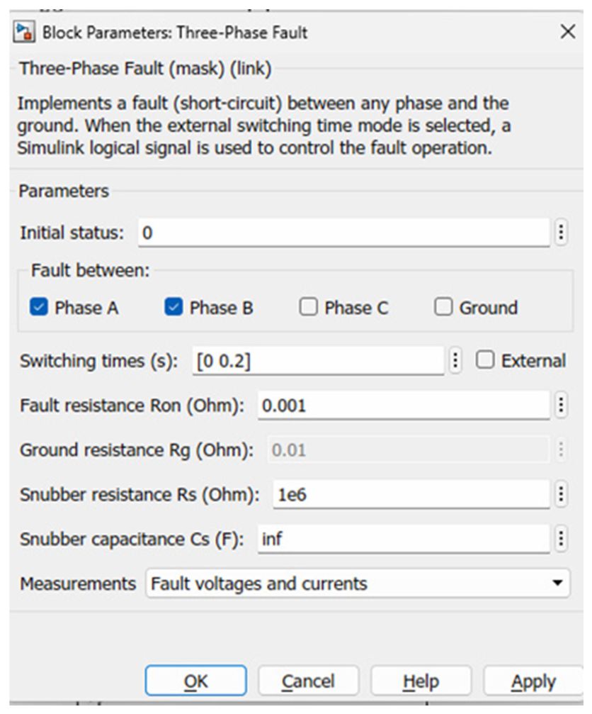
The test systems used are standard fault testing systems known as the IEEE 9-bus system [17,18] and the IEEE 30-bus system [23,24]. In the IEEE 9-bus test system, there are three generators connected with nine buses and six transmission lines; the connection and all the details of the IEEE 9-bus system are given in Figure 1. In the IEEE 30-bus test system, there are 30 buses, 6 generators, 4 transformers, and 41 transmission lines, as indicated in Figure 2. In Table 1, the fault simulation parameters of the IEEE 30-bus system are provided. Research in the field of power flow analysis, economic dispatch, and power system analysis are some of the areas where these test systems are used. Both IEEE 9-bus and IEEE 30-bus systems have been implemented using a 100 MVA system base and an operating frequency of 60 Hz. The sampling frequency is 20 kHz. The physical properties of the transmission lines and load characteristics were taken from books and references [17,18,23,24,25]. The IEEE 9-bus and IEEE 30-bus systems were adopted as benchmark networks for generating the fault database. The transmission networks were subsequently implemented in MATLAB/Simulink [22]. For fault data generation, the electrical distance from the location of the fault was varied over fault locations km. In order to model a fault at a new location on the transmission line between the two buses, the fault details in the three-phase fault block are changed, such as fault time, fault resistance, and fault type and location on the transmission line, as illustrated in Figure 3.

Table 1. System and parameters for fault simulation.

System Parameters	Values
Test systems	IEEE 9 and IEEE 30 bus systems
fault distance (km)	100, 121, 75, 177, 200, 21, 25, 33, 49, 56, 50
Fault type	Line-to-ground, line-to-line, and double line-to-ground
Features	DWT features, voltage, current
Frequency (Hz)	60
Fault resistance (ohms)	0.001
Switching time (s)	0–0.2

Figure 3. Three-phase fault parameters [22].

Asymmetrical faults: the line-to-ground, line-to-line, and double line-to-ground faults for all the phases have been simulated in this work. The most recurring faults in the power system are asymmetrical faults, which lead to interruption of power supply [26]. In the IEEE 9-bus system, the faults were generated between buses 7 and 8, and the post-fault voltage and current data were collected from bus 7. In the IEEE 30-bus system, faults of diverse types were generated between buses 4 and 6, and the post-fault voltage and current data were acquired at bus 6. The fault conditions consist of line-to-ground faults (L-G), Phase A to ground (A-G), Phase B to ground (B-G), and Phase C to ground (C-G) at various points such as 100 km, 75 km, 121 km, 177 km, 21 km, 33 km, and 56 km, and so on. Likewise, faults at transmission lines were created with double-line faults at different locations. Under various conditions, double-line-to-ground faults are created. The post-fault voltage signal and current are produced and passed to the workspace to be analyzed further by DWT.

2.2. Data Acquisition and Feature Simulation

After performing fault simulation in the IEEE 9-bus system and IEEE 30-bus transmission system. Faults at various locations were generated; corresponding three-phase voltage and current were accumulated at bus number 7 and bus number 6 from the IEEE 9-bus and 30-bus systems, respectively. Therefore, the reference points for IEEE 9 and IEEE 30 are bus no. 7 and bus no. 6. From each simulation, 6 features were initially obtained. Each fault is generated at 11 different locations, and data are collected for 9 different faults. These data include three-phase voltages, three-phase currents, and corresponding time. Approximately 40,000 data samples were obtained from the 99 simulated fault cases; these individual samples were not considered statistically independent fault experiments because samples originating from the same simulation may exhibit correlation. To prevent information leakage between the training and testing datasets, data partitioning was, therefore, performed at the fault case level rather than at the individual sample level. Each simulation case was assigned a unique identifier according to its fault location and fault type. All samples extracted from the same simulation were associated with the same case identifier and were allocated exclusively to one subset. For example, if the samples generated from an AG fault at 121 km were assigned to the training set, no samples originating from that same AG fault simulation at 121 km were included in the validation or testing sets. Thus, samples belonging to a particular simulation case were never distributed across different subsets, ensuring that the model was evaluated using fault cases that were not used during model training. This group-wise partitioning strategy minimizes the influence of correlation between samples from the same simulation and provides a more reliable assessment of the model’s generalization performance. This way, the data is further divided into training and testing samples. The current data for each signal obtained for each fault is then processed using the discrete wavelet transform (DWT) to extract transient detail coefficients for each generated post-fault current.

2.2.1. Detailed Coefficients Using DWT

When a fault happens, high-frequency transients may be generated and propagate at the terminals of transmission lines [27]. Within the wavelet transform, the time-dependent functions dubbed wavelets change the time scale based on their spectral content. For high-frequency wavelets, time widths are very narrow, unlike the environment with low-frequency wavelets, which have large time widths. This multi-resolution property is particularly desirable in fault transient analysis, where the transient nature of fault analysis is often dominated by high-frequency components that are localized about the basic power frequency decomposition. It follows that the wavelet transform is naturally better suited to study signals whose disturbances have a short period and high frequency [28]. In each fault instance between buses 7 and 8 in the IEEE 9-bus test system and buses 4 and 6, post-fault current data at bus 7 in the IEEE 9-bus system and at bus 6 in the IEEE 30-bus system are recorded and processed with DWT. It is obtained in the form of the mathematical expression given in Equation (1).

$$DWT\left(f,m,n\right)={\displaystyle \frac{1}{\sqrt{a_0^m}}} {\sum }_{k}f\left(k\right){\Psi }^{*}\left({\displaystyle \frac{n-k{a}_0^m}{a_0^m}}\right)$$

(1)

The parameters m and n are the scale and translation indices; f (k) is an input signal. ${\Psi }^{*}$ is the complex conjugate of the mother wavelet. ${\displaystyle \frac{1}{\sqrt{a_0^m}}}$ is a scaling term that normalizes the energy across different scales. $\sum _{k}f\left(k\right){\Psi }^{*}$ is a discrete inner product that correlates the signal with a scaled or shifted wavelet. A third-level decomposition wavelet transform is applied in this study to obtain desirable time-frequency features to extract the current signals Ia, Ib, and Ic to identify fault position. The DWT is implemented with the use of Daubechies-4 (db4) mother wavelet as it is compactly supported, orthogonal, and suitable for detecting transients in power system signals [29]. Practical implementation of the DWT proceeds in a complementary manner by recursively passing the input signal through a low-pass analysis filter and a high-pass analysis filter, and then downsampling. For each decomposition level, the low-pass branch generates an approximation component which contains the lower frequencies. The high-pass branch, on the other hand, generates a detail component with local high-frequency information. The filtered and decimated approximation is provided to the next step of decomposition. Consequently, higher-frequency bands yield level-1 details, and a lower high-frequency band yields level-3 details, which yield better localization. The hierarchical arrangement allows localization of transient features as well as their global capture. For each phase current, the DWT is applied to the input using MATLAB’s function wavedec, which outputs a coefficient vector, a single row vector and a vector containing the approximation coefficient length and detail coefficient length at each level. The final low-frequency representation, level-3 approximation, is obtained by the function appcoef and the high-frequency details at levels 1, 2 and 3 are produced by the function detcoef. This provides sets of detailed coefficients for each phase, one set for each frequency band. Each phase is combined to obtain a single feature array that is the detail coefficient (D), which is the level-3 detail coefficients for a short-duration, high-frequency disturbance when acting as the fault transient characteristic. The detail coefficients of this signal are generated for each fault occurring at different locations and tabulated. This way, we obtained nine features, including voltage, current and three DWT coefficients.

2.2.2. Detailed Engineered Features

In order to increase fault location sensitivity and feature separability, some features have been generated by applying various calculation processes to the original data features, which are post-fault voltage and current. Raw features are nine, including post-fault voltage and current for all three phases and three detailed coefficients. Using raw post-fault voltage, we calculated further features and included them while simulating each model. These engineered features include apparent power and its components for all original features, voltage and current magnitude, impedance-based features, Clarke transform component, Clarke transform current component, Clarke transform voltage component, Clarke magnitude, current-voltage interaction index, impedance index.

For each generated fault, 27 different features are constructed from single-ended three-phase voltage and current measurements. The first six input features are three-phase voltage and current features, which are values recorded for the fault signal. DWT coefficients are calculated using the DWT. Voltage and current magnitudes are calculated from phase voltage and current; apparent power and impedance are calculated using voltage and current. However, a small stabilization constant ε (epsilon) is added when a phase drops to zero. An amplitude-invariant Clarke transformation is used to transform the phase measurement domain into stationary (Vα, Vβ, and V0) coordinates. Using the Clarke transformation components, the corresponding Clarke magnitude generates Vαβ and Iαβ. The rest of the features show the geometric and impedance relationship of voltage-current interaction in the Clarke plane, as shown in Table 2 below.

Table 2. The engineered features and their mathematical definition.

Features	Mathematical Definition
Three-phase voltage and current	[Va, Vb, Vc] [Ia, Ib, Ic]
DWT coefficients	[Da, Db, Dc]
Voltage and current magnitude	$\mathrm{V}\mathrm{m}=\sqrt{{\mathrm{V}\mathrm{a}}^2+\mathrm{V}{\mathrm{b}}^2+\mathrm{V}{\mathrm{c}}^2},$$\mathrm{I}\mathrm{m}=\sqrt{{\mathrm{I}\mathrm{a}}^2+\mathrm{I}{\mathrm{b}}^2+\mathrm{I}{\mathrm{c}}^2}$
Apparent power and impedance	Sa = ∣Va Ia∣, Sb =∣Vb Ib∣, Sc =∣Vc Ic∣, $\mathrm{Z}\mathrm{a}={\displaystyle \frac{\left|\mathrm{V}\mathrm{a}\right|}{\left|\mathrm{I}\mathrm{a}\right|+\mathsf{\epsilon }}}\hspace{1em}\mathrm{Z}\mathrm{b}={\displaystyle \frac{\left|\mathrm{V}\mathrm{b}\right|}{\left|\mathrm{I}\mathrm{b}\right|+\mathsf{\epsilon }}}\hspace{1em}\mathrm{Z}\mathrm{c}={\displaystyle \frac{\left|\mathrm{V}\mathrm{c}\right|}{\left|\mathrm{I}\mathrm{c}\right|+\mathsf{\epsilon }}}$
Clark transform	$\left[\begin{array}{c}{\mathrm{V}}_{\mathsf{\alpha }}\\ {\mathrm{V}}_{\mathsf{\beta }}\\ {\mathrm{V}}_0\end{array}\right]={\displaystyle \frac{2}{3}}\left[\begin{array}{ccc}1& {\displaystyle \raisebox{1ex}{$-1$}\!\left/ \!\raisebox{-1ex}{$2$}\right.}& {\displaystyle \raisebox{1ex}{$-1$}\!\left/ \!\raisebox{-1ex}{$2$}\right.}\\ 0& {\displaystyle \raisebox{1ex}{$\sqrt{3}$}\!\left/ \!\raisebox{-1ex}{$2$}\right.}& {\displaystyle \raisebox{1ex}{$-\sqrt{3}$}\!\left/ \!\raisebox{-1ex}{$2$}\right.}\\ {\displaystyle \raisebox{1ex}{$1$}\!\left/ \!\raisebox{-1ex}{$2$}\right.}& {\displaystyle \raisebox{1ex}{$1$}\!\left/ \!\raisebox{-1ex}{$2$}\right.}& {\displaystyle \raisebox{1ex}{$1$}\!\left/ \!\raisebox{-1ex}{$2$}\right.}\end{array}\right]\left[\begin{array}{c}\mathrm{V}\mathrm{a}\\ \mathrm{V}\mathrm{b}\\ \mathrm{V}\mathrm{c}\end{array}\right]$ $\left[\begin{array}{c}{\mathrm{I}}_{\mathsf{\alpha }}\\ {\mathrm{I}}_{\mathsf{\beta }}\\ {\mathrm{I}}_0\end{array}\right]={\displaystyle \frac{2}{3}}\left[\begin{array}{ccc}1& {\displaystyle \raisebox{1ex}{$-1$}\!\left/ \!\raisebox{-1ex}{$2$}\right.}& {\displaystyle \raisebox{1ex}{$-1$}\!\left/ \!\raisebox{-1ex}{$2$}\right.}\\ 0& {\displaystyle \raisebox{1ex}{$\sqrt{3}$}\!\left/ \!\raisebox{-1ex}{$2$}\right.}& {\displaystyle \raisebox{1ex}{$-\sqrt{3}$}\!\left/ \!\raisebox{-1ex}{$2$}\right.}\\ {\displaystyle \raisebox{1ex}{$1$}\!\left/ \!\raisebox{-1ex}{$2$}\right.}& {\displaystyle \raisebox{1ex}{$1$}\!\left/ \!\raisebox{-1ex}{$2$}\right.}& {\displaystyle \raisebox{1ex}{$1$}\!\left/ \!\raisebox{-1ex}{$2$}\right.}\end{array}\right]\left[\begin{array}{c}\mathrm{I}\mathrm{a}\\ \mathrm{I}\mathrm{b}\\ \mathrm{I}\mathrm{c}\end{array}\right]$
Clark magnitude	$\mathrm{V}\mathsf{\alpha }\mathsf{\beta }=\sqrt{{\mathrm{V}\mathsf{\alpha }}^2+\mathrm{V}{\mathsf{\beta }}^2},\mathrm{I}\mathsf{\alpha }\mathsf{\beta }=\sqrt{{\mathrm{I}\mathsf{\alpha }}^2+\mathrm{I}{\mathsf{\beta }}^2}$
Current-voltage direct interaction	Pαβ = Vα Iα + Vβ Iβ
Current-voltage cross interaction	Qαβ = Vβ Iα − Vα Iβ
Current-voltage interaction index (CVII)	$\mathrm{C}\mathrm{V}\mathrm{I}\mathrm{I}={\displaystyle \frac{{\mathrm{V}}_{\mathsf{\alpha }}{\mathrm{I}}_{\mathsf{\alpha }}+{\mathrm{V}}_{\mathsf{\beta }}{\mathrm{I}}_{\mathsf{\beta }}}{{\mathrm{V}}_{\mathsf{\alpha }\mathsf{\beta }}{\mathrm{I}}_{\mathsf{\alpha }\mathsf{\beta }}+\mathsf{\epsilon }}}$
Impedance index	${\mathrm{Z}}_{\mathsf{\alpha }\mathsf{\beta }}={\displaystyle \frac{{\mathrm{V}}_{\mathsf{\alpha }\mathsf{\beta }}}{{\mathrm{I}}_{\mathsf{\alpha }\mathsf{\beta }}+\mathsf{\epsilon }}}$

The entire feature dataset was designed to extract both transient and characteristic features associated with the fault distance to improve the learning capability of the machine learning and deep learning models. After feature extraction and data preprocessing, the final dataset consisted of approximately 40,000 samples, with each sample represented by 27 input features and an associated continuous fault-location target. The 27-dimensional feature set comprised the electrical measurements, DWT-derived information, and engineered electrical features described above. All 27 features were retained for model development, and no additional feature-selection procedure was applied. Because multiple samples were extracted from each simulated fault case, samples originating from the same simulation were treated as a group during dataset partitioning to prevent information leakage between the training and testing sets. Each simulation case was assigned a unique identifier according to its fault conditions, and all samples associated with a given case were allocated exclusively to one data subset. The data were divided into approximately 80% for training and 20% for independent testing, with a validation subset obtained from the training data using a holdout procedure for hyperparameter optimization and model selection. Normalization parameters were calculated exclusively from the training data and subsequently applied unchanged to the validation and test data. The independent test data were not used during model training, normalization-parameter estimation, hyperparameter optimization, or model selection and were used only for the final assessment of model generalization performance. All 27 engineered features were retained as inputs to the learning models, and no feature elimination or feature selection procedure was applied. Specifically, the features were not removed on the basis of correlation thresholds, minimum relevance criteria, or feature importance rankings. Correlation analysis and feature-importance metrics were, therefore, not used as criteria for constructing the 27-feature input set. The same complete feature set was provided to all models to ensure a consistent basis for model comparison.

3. Machine Learning and Deep Learning-Based Fault Location

3.1. Convolutional Neural Network-Based Fault Location

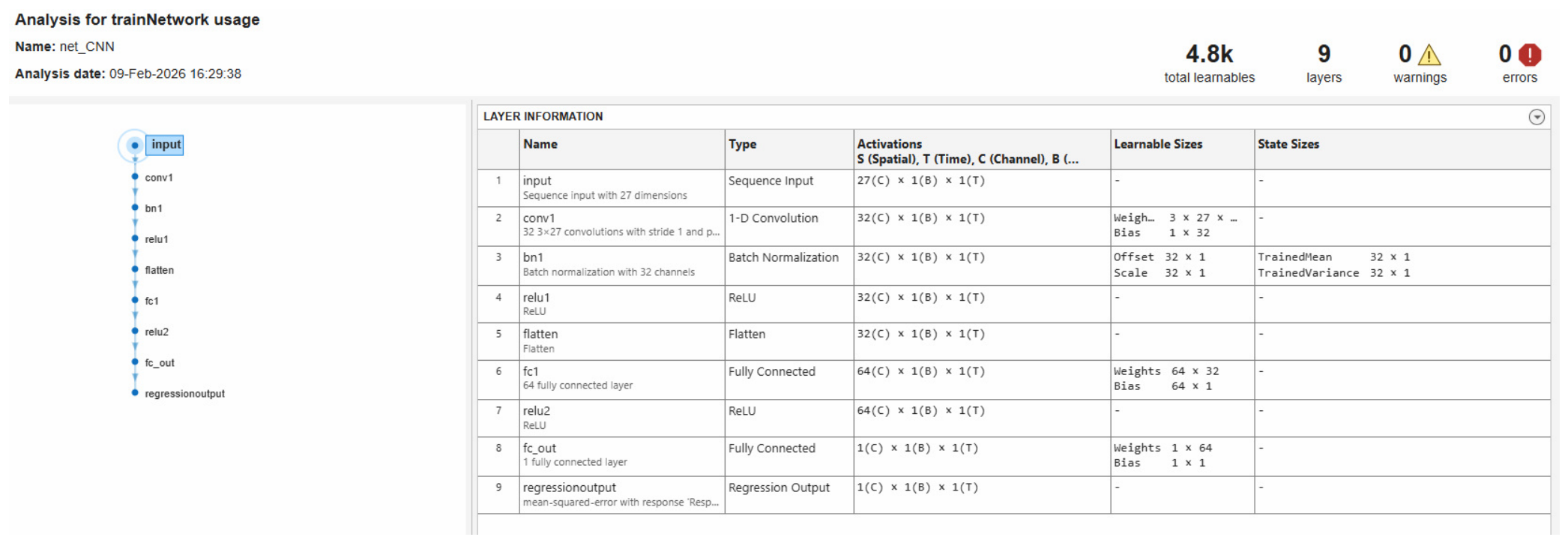
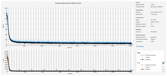
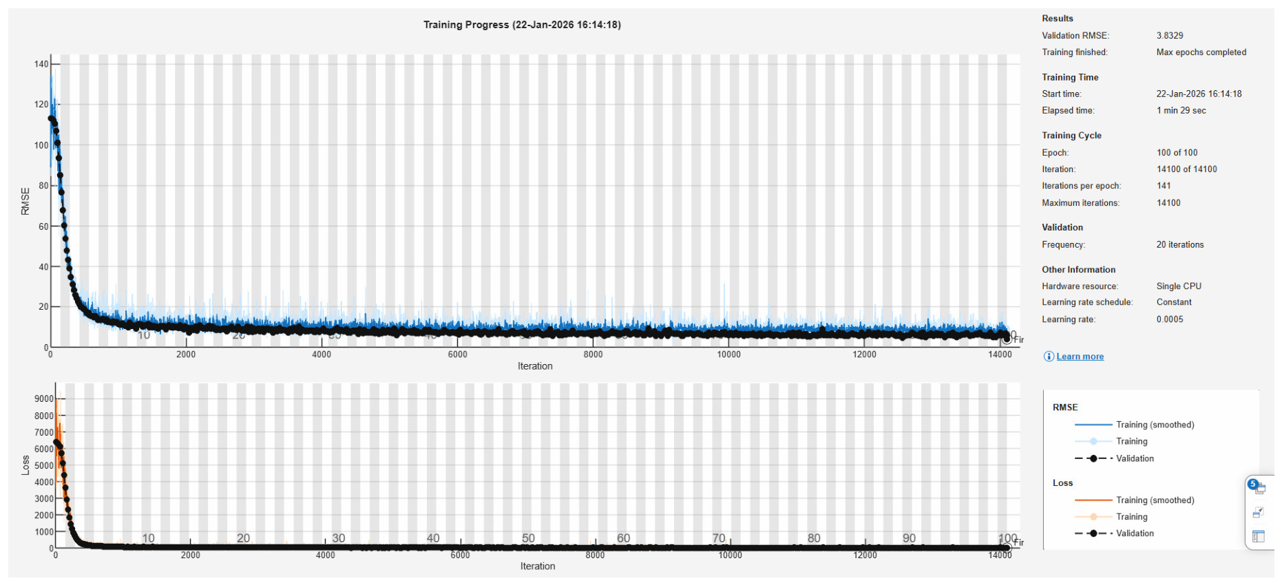
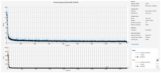
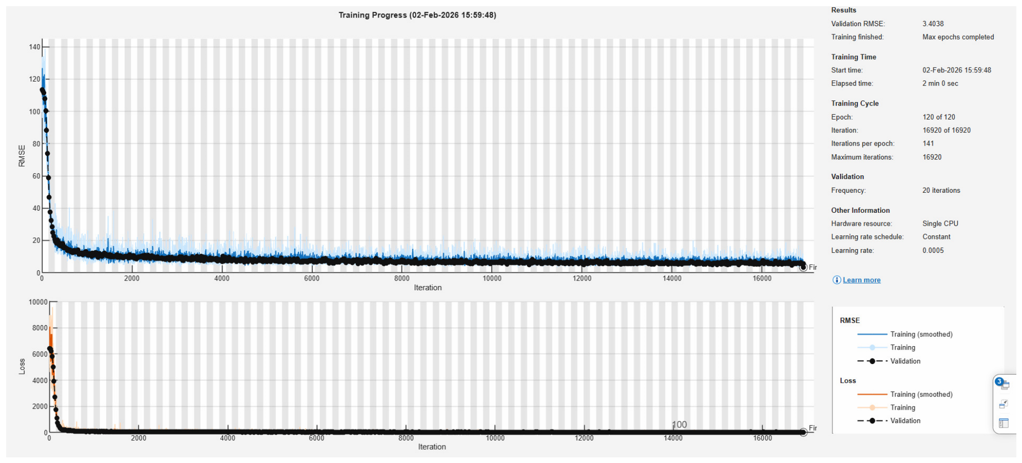
Machine learning and deep learning models are developed to test and compare fault location in the IEEE 9-bus system and IEEE 30-bus system. The proposed deep learning model is a CNN, which is used and modified to develop a relationship between different features of the fault and the fault location. CNNs are excellent for modeling complex mappings onto structured data, as they can be built with layers of connectivity that are sparse, and parameters are shared in terms of connectivity [30,31]. The CNN, with the DWT coefficients as the input, is able to achieve decent efficiency in learning the functional relationship between these computed features and the fault location without any loss of information, further breaking down the features into multiple scales [32]. To handle the original nine features and an augmented 18-feature vector made up of three-phase voltages, three-phase currents, and DWT coefficients, apparent power, magnitude for voltage and current, apparent impedance [33], transient energy, Clarke transform current component, Clarke transform voltage component, Clarke magnitude, current-voltage interaction index, impedance index calculated from fault current and voltage signal. The convolutional layer is able to capture the local relationships among voltage, current, and multi-scale DWT coefficients, which can be used for fault distance estimation by feeding the sequence of time-domain features as a 1D sequence. The CNN with different layers designed in this study is displayed in Figure 4. Each sample is represented by a 1 * 27 feature vector in the first sequential layer; the input of the network contains the nine original features, three phase currents and three voltages, as well as the DWT coefficient and 18 augmented features for a total of 27 features. The design is similar to the one adopted in the power system, where structured feature vectors are fed into the convolutional regression model [34]. A sequential layer is followed by a 32 × 3 1D Convolutional layer learning the transients of voltage and current from one phase to another, and correlations of DWT coefficients. Convolutional layers are good at capturing structured feature patterns; therefore, they are effective for fault analysis [35,36]. A batch normalization layer is employed to stabilize the internal features, which enhances the stability of training for the power system models. A ReLU and a flatten layer are used to make the model non-linear and to flatten the multi-channel convolutional output to a vector, thus allowing it to integrate and interpret the extracted features in the fully connected layers [37,38]. In addition, two convolutional layers with the ReLU activation function are added and, finally, a regression layer to minimize the mean squared error [39,40]. According to [41], for details of the Adam optimizer, which adaptively resets the learning rate for every parameter and has shown good convergence properties for approximating nonlinear electrical signals. We use four learning rates, 10⁻², 5 * 10⁻³, 10⁻³, 5 * 10⁻⁴ to prevent suboptimal convergence. An optimal search for the validation RMSE, as shown in the training progress graph in Figure 5, is fundamental in deep learning of power systems to prevent overfitting during hyperparameter optimization [42]. The CNN was configured with a kernel size of 3 and 32 filters and contained approximately 4.8K trainable parameters. These architectural settings were fixed during the experiments, while the validation set was used for optimization of the designated training hyperparameters.

Figure 4. CNN trained model and detailed layers [22].

Figure 5. CNN model training and validation progress [22].

3.2. LSTM-Based Fault Location

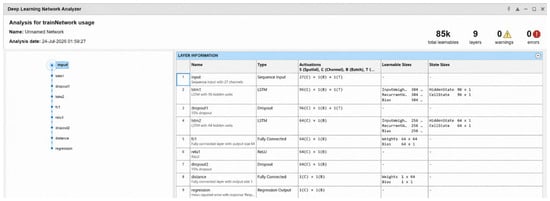
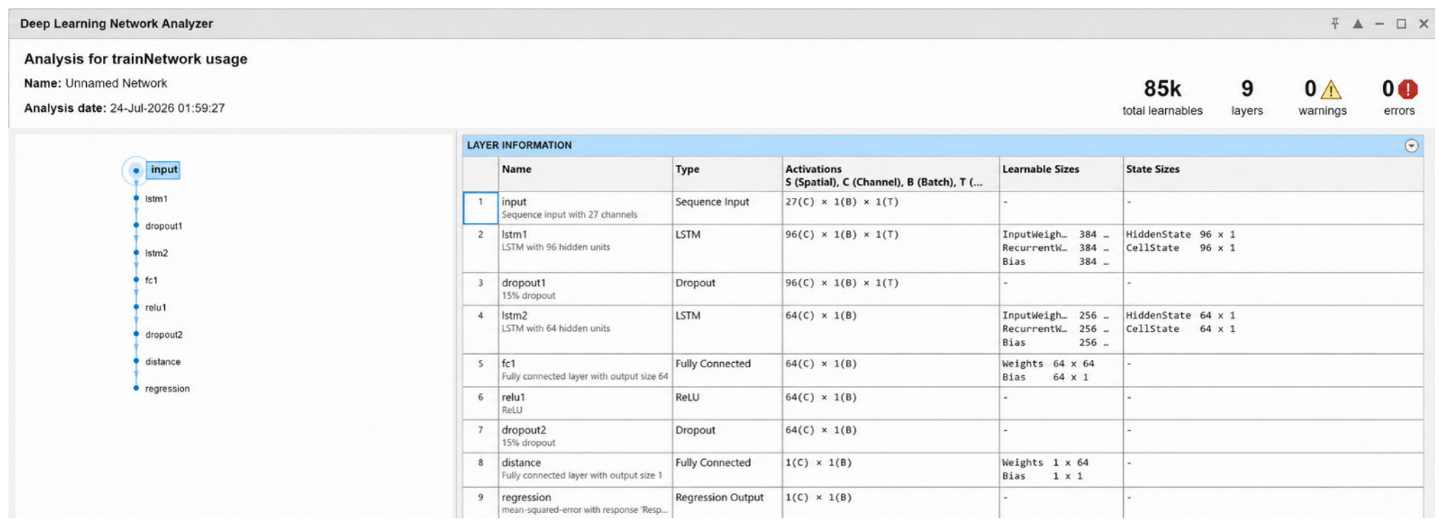
CNNs are very good at capturing local spatial interactions among the voltage, current, and all fault features. LSTMs are good at capturing the lengthy time features and nonlinear interactions among the components in a sequence [43,44]. This algorithm is able to learn patterns to identify a fault. The sequence to be processed is the feature vector of voltage, current and DWT. The local interactions between features become a sequential, mutually dependent chain of features and are interpreted by LSTM. Previous studies have shown that the LSTM is more effective in the literature for the transient analysis and fault detection of power systems [45,46,47]. As shown in Figure 6, the construction of the LSTM starts with the sequence input layer; it takes 1*27 features, including voltage, current and DWT coefficients and augmented 18 features, including apparent power, magnitude for voltage and current, apparent impedance, transient energy, Clarke transform current component, Clarke transform voltage component, Clarke magnitude and current-voltage interaction index. The impedance index is used as an input sequence [48]. Multiple LSTM layers are used. The second layer is the first LSTM layer with 96 memory units. Each unit has an input gate, forget gate, output gate, and cell state. This layer learns the patterns. LSTM has gained popularity with the great prospect of learning a hierarchy of short feature vectors [37,43]. The next layer is the first dropout layer, which looks after overfitting by reducing the activations during the process of training and improves generalization. The next layer is the second LSTM layer, which represents the patterns related to the fault location. This LSTM layer has 64 memory cells. The mathematical representation of the output is given as the forget cell, input cell, output cell, memory update and hidden gate and is mathematically represented as Equations (2)–(7).

$$f_t=\sigma \left(W_f{x}_t+W_f{h}_{t-1}+b_f\right)$$

(2)

$$i_t=\sigma \left(W_i{x}_t+W_i{h}_{t-1}+b_i\right)$$

(3)

$$o_t=\sigma \left(W_o{x}_t+W_o{h}_{t-1}+b_o\right)$$

(4)

$$a_t=tanh\left(W_a{x}_t+W_a{h}_{t-1}+b_a\right)$$

(5)

$$c_t=f_t\ast c_{t-1}+i_t\ast \sigma \left(W_c{x}_t+W_c{h}_{t-1}+b_c\right)$$

(6)

$$h_t=o_t\ast {\sigma }_h\left(c_t\right)$$

(7)

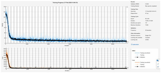
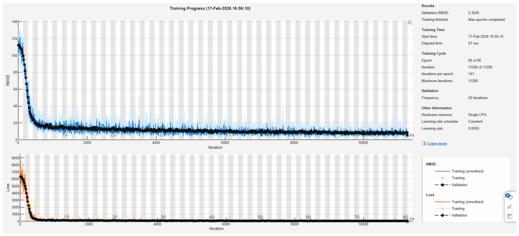
where $f_t$, ${\mathrm{i}}_{\mathrm{t}}$, ${\mathrm{o}}_{\mathrm{t}}$are forget, input, and output gate vectors, $a_t$is the internal vector, and $W_t$, $W_i$, $W_o$, $W_a$ are the weights of the respective input and output gates for training on the data. The $c_t$is the memory cell state and $h_t$ is the hidden state of the LSTM. The symbol $b_f, b_i, b_o, b_a,$represents the output bias values. The intent of this layer in this design is to learn the pattern of dependencies between voltage features, current features, DWT features, and voltage versus current versus DWT coefficient variations, as well as nonlinear conditional relationships. It gathers global contextual information, boosts generalization performance and enhances the stability of prediction. LSTMs are used in transient analysis [44,49,50]. The LSTM layer is followed by a fully connected layer. After this layer, ReLU is used for nonlinear activation of the network in order to train the network due to the removal of vanishing gradients [51]. This is then followed by a second dropout layer for further regularization. Next to this is another and final fully connected output layer to produce the predicted distance as the fault location. This is then followed by a regression layer as the output layer, which compares the previous layers’ predicted distance with the actual distance and generates and minimizes the MSE. The Adam optimizer is used in the LSTM; it is highly effective and adaptively learns the learning rates of all the parameters [41]. Learning rate normalization is set at different rates, such as 10⁻², 5 * 10⁻³, 10⁻³, 5 * 10⁻⁴ and the batch size is 32, with validation-based early stopping. To reduce overfitting. The trained LSTM structure is given in Figure 6; the training and validation are given in Figure 7.

Figure 6. LSTM trained model and detailed layers [22].

Figure 7. LSTM model training and validation progress [22].

3.3. BiLSTM-Based Fault Location

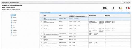
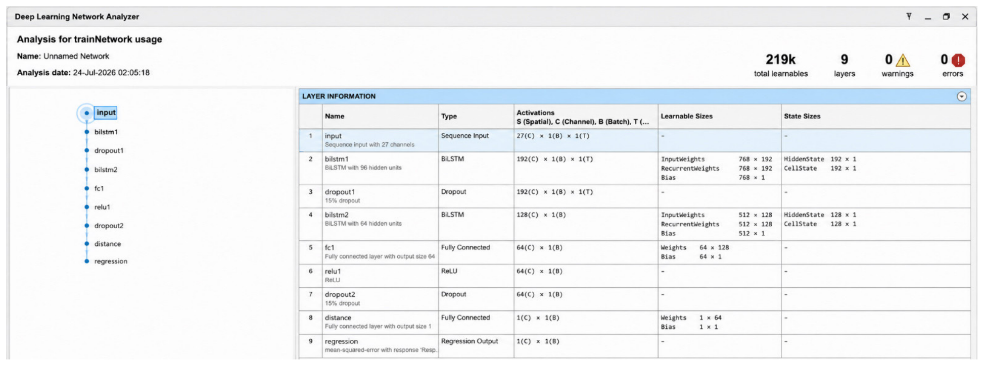
BiLSTM is a network that combines bidirectional LSTM, which learns forward and backward dependencies in the feature and learns local spatial correlations in the feature vector. BiLSTM layers study the forward and backward contexts, which is more comprehensive than a simple LSTM. The hybrid structure has been proven to be superior in the power system fault diagnosis (PSFD) tasks in various studies [43,44,45,46]. In this paper, we present an input layer of a 1×27 feature sequence. The total number of original features is 9 and the augmented features are 18. So the total number of features is 27, as mentioned in Figure 8. By considering the features as a sequence, the BiLSTM can learn the context dependency from the features, based on voltage and current features, thus achieving better mapping accuracy for locating fault positions. Our structure begins with an input layer, which takes nine original features: three voltages and three current profiles, and three initial DWT coefficients, as well as 18 augmented features. This first input sequence layer extracts the features’ correlations. Its mathematical representation can be written as shown below in Equation (8).

$$F_t=\sigma \left(W\ast X_{t:t+2}+b\right)$$

(8)

Figure 8. BiLSTM trained model and detailed layers [22].

During this layer, learning of the nonlinear relationship between spatial relationships is realized; feature intersections are captured, noise is reduced and fault information is enhanced. The feature extraction is employed in hybrid models for fault analysis [22,40]. It is followed by the first BiLSTM layer, which contains 96 memory units. This layer processes the input for all the samples using forward LSTM and backward LSTM and it combines the outputs; therefore, the output becomes twice the number of features it received at each unit. The next layer is a dropout layer, which improves generalization ability by overcoming overfitting. After this layer is the second BiLSTM layer with 64 forward memory units and 64 backward memory units. The main component in this layer is a bidirectional LSTM, which processes the input in both directions. In terms of mathematics, it is represented by the forward recurrence Equation (9).

$${\overrightarrow{h}}_t=LSTM\left(x_t,\overrightarrow{h_{t-1}}\right)$$

(9)

Equation (10) for the backward process is shown as

$${\overleftarrow{h}}_t=LSTM\left(x_t,\overleftarrow{h_{t+1}}\right)$$

(10)

The final hidden state can be represented as an Equation (11)

$$h_t=\left[{\overrightarrow{h}}_t:{\overleftarrow{h}}_t\right]$$

(11)

The advantages of BiLSTM are that it models dependencies with respect to both past and future and models all the dependencies between features. For complex nonlinear mapping, such as fault analysis, results have shown BiLSTM to be very effective [44,49,50]. A fully connected layer is added after the BiLSTM layer to combine the BiLSTM hidden state with the feature space. A fully connected layer is followed by another ReLU layer to map more precisely. A second dropout layer is added before the final fully connected layer for regularization. A fully connected layer is followed by the regression layer for the final fault prediction output. Lastly, the regression layer is employed to calculate and compare the RMSE and to minimize it. The trained structure of BILSTM is presented in Figure 8 and the training and validation details are shown in Figure 9. The input to the LSTM and BiLSTM networks consists of 27 feature channels derived from the measured voltage and current signals, DWT coefficients, and the corresponding engineered electrical features. The 27 features are not interpreted as 27 consecutive temporal steps. In the implemented network, they constitute the feature dimension of the sequence input. The recurrent layers are employed to learn dependencies within the ordered representations obtained from the fault-signal records and to map these representations to the continuous fault location target. Thus, the feature dimension and the sequence dimension are treated separately, avoiding the interpretation of heterogeneous electrical features as successive physical time instants.

Figure 9. BiLSTM model training and validation progress [22].

3.4. Backpropagation Neural Network

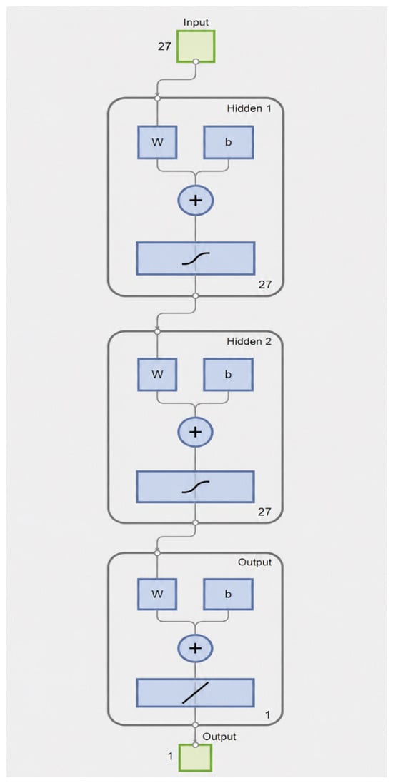
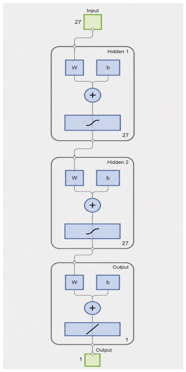
Artificial neural networks (ANNs) are known for their ability to provide robust solutions for fault detection and fault classification, and therefore, they have wide application in fault diagnosis in complex power systems. Their capability of learning and approximation is especially good for the problem of fault analysis involving non-linearity and complicated components. By learning from data, ANNs can adapt to changing operating conditions and make better decisions, which they would be able to do without training. Due to these characteristics, they are widely used in the area of fault identification [52]. Backpropagation neural networks work without having thorough expertise of the network, as it is simple, quick, and straightforward to implement [7,41]. The neural network we developed for this work is a Levenberg–Marquardt backpropagation neural network with an input layer and two hidden layers and one output layer, as shown in Figure 10. This network is designed using the nnstart tool in MATLAB. The data generated from the IEEE 9- and IEEE 30-bus systems is fed into the input layer, and the labeled output, which is the distance at which the fault is generated, is updated as output along with parameters such as each layer’s activation functions and neurons in the layers. Once we start the process of training, the RMSE and MAE are generated each time and compared with the target output; if the difference is too high, it adjusts the weights and bias values and runs again until it achieves the error target. That is when the model is ready to be tested with the test data. Once it is ready, it is tested with the unseen data from the IEEE 9-bus and IEEE 30-bus systems to generate the results and validate its performance. The mathematical expression for achieving the output at each epoch is given in Equation (12) [3].

$$y_j={\displaystyle \sum _{j=1}^n}{\omega }_{k,j }f\left(h_k\right)+{\beta }_j$$

(12)

Figure 10. ANN structure for fault location [22].

The ${\omega }_{k,j }$ is the weight of node k at epoch number j. ${\beta }_j$ is the bias value of the output node at epoch j. $f\left(h_k\right)$ is the output value of hidden node k. The fitness values can be calculated using the error in Equation (13) below.

$$Fitness\left(y_j\right)=minimum\left(RMSE\right)$$

(13)

The ANN consisted of 27 input features, two hidden layers containing 27 neurons each, and one output neuron. The hyperbolic tangent sigmoid (tansig) transfer function was employed in both hidden layers, while a linear (purelin) transfer function was used in the output layer for fault location. The network was trained using trainlm with MSE as the performance function, and training was terminated when the predefined performance goal of net.trainParam.goal = 1 × 10⁻³ was achieved, and the maximum number of training epochs was set to 1000.

3.5. Adaptive Neuro Fuzzy Inference System

ANFIS is a hybrid algorithm that uses the ANN for self-learning and fuzzy logic for knowledge-based learning [53]. Each node performs independently of other nodes; therefore, it is capable of differentiating each feature and generating the output for each input. Better generalization ability and better decision-making ability make it suitable for complex tasks like predicting the location of faults in power systems. The tuning in this technique was conducted for the membership functions and the number of membership functions. There are five layers in the ANFIS. Each layer performs some function to update the values of input and output. The layer description is given as follows: in layer 1, each node has a node function. It generates the membership grade as an output and it is given by Equation (14).

$$O_i^1=\mu A_i\left(x\right)$$

(14)

where A is the label connected to the node. $O_i^1$ is the membership function of $\mu A_{i }\left(x\right)$.

In layer 2, the nodes are fixed; each node performs a multiplier function. The symbol π denotes the multiplier. Each node in this layer multiplies the input signals to obtain the firing strength of each rule as output. Equation (15) is written as follows [54]

$$O_i^2=w_i={\pi }_{j=1}^m\mu A_i\left(x\right)$$

(15)

In layer 3, nodes are fixed in this layer as well. Normalization of the firing strength, which is the output from the previous layer, takes place. The equation for this layer is given as Equation (16).

$$O_i^3=\overline{w}={\displaystyle \frac{w_i}{w_1+w_2}}$$

(16)

At layer 4: each node in this layer is not fixed is an adaptive node, and the output parameters are changed in this layer. The output combines the first-order polynomial with the normalized firing strength; this is conducted for each node in the layer. As a result, each node at this layer outputs as in Equation (17).

$$O_i^4=y_i=\overline{W_i}{f}_i=\overline{W_i}\left(p_i{x}_1+q_i{x}_2+r_i\right),i=\mathrm{1,2},..$$

(17)

At layer 5, all the inputs from the previous layer are summed together to obtain the predicted output. The total sum of the output is given by Equation (18).

$$O_1^5={\sum }_i{y}_i={\sum }_i\overline{w_i}{f}_i=\overline{w_1}\left(p_1{x}_1)+{\overline{w_1}(q}_1{x}_2)+({\overline{w_1}r}_1\right)+\overline{w_2}\left(p_2{x}_2)+{\overline{w_2}(q}_2{x}_2)+({\overline{w_2}r}_2\right)$$

(18)

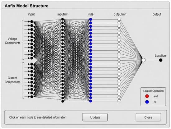
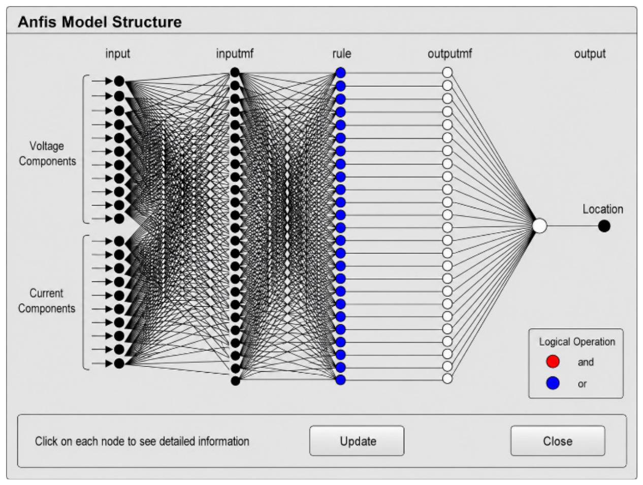
The following parameters are solved using a least-squares technique in this final layer. The final equation can be written as Equation (19). The ANFIS structure with all five layers are presented in Figure 11. The ANFIS model was implemented using a Sugeno-type fuzzy inference system generated using subtractive clustering.

$$y=\left[w_1{x}_1 w_1{x}_{2 }{ w}_1 w_2{x}_{2 } w_2\right]\left[\begin{array}{c}{p}_1\\ q_1\\ r_1\\ p_2\\ q_2\\ r_2\end{array}\right]=XW$$

(19)

Figure 11. ANFIS structure for fault location [22].

The input variables were represented using Gaussian membership functions. The subtractive clustering resulted in 50 clusters, with each cluster corresponding to one fuzzy rule. Therefore, the resulting FIS contained 50 fuzzy rules and 50 clusters with Gaussian membership functions for each input variable. The implemented FIS consisted of 27 input variables and one output representing the estimated fault location. The product operator was employed for the AND operations, probabilistic OR for the OR operation, sum for aggregation, and weighted average defuzzification was used to obtain the output.

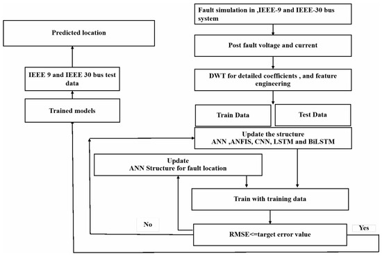
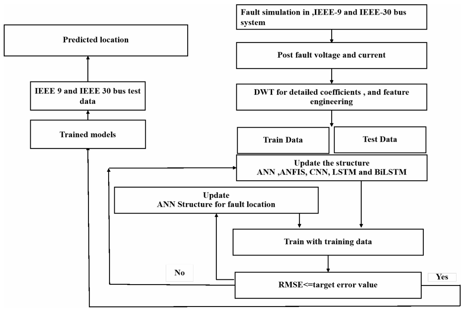
A Fault simulation is conducted at several locations on the transmission lines of the IEEE 30- and IEEE 9-bus systems, and the corresponding values of the voltage and the current at the buses are recorded. The post-fault current signal is subsequently decomposed by DWT to obtain the detailed coefficients. Moreover, these coefficients are added to the raw fault voltage and fault current values and processed to create other features. Based on this dataset, three deep learning architectures are built for fault detection. The data are split into two sets: training data and testing data. The parameters to be tuned are updated based on the RMSE value and the trained models are tested with the test data to check the model efficiency. The trained models are tested with the test data and random data generated from the IEEE 9-bus and IEEE 30-bus systems at various locations. The details of all the models are given in Table 3. The detailed results, including RMSE, MAE, and percentage error of the model, are shown in Table 4 and Table 5.

$$RMSE=\sqrt{{{\displaystyle \frac{1}{n}}{\displaystyle \sum _{i=1}^n} \left({Output}_{predicted}-{Output}_{actual}\right)}^2 }$$

(20)

$${ R}^2=1-{\displaystyle \frac{ {\displaystyle {\sum }_{i=1}^n}{\left({Output}_{predicted}-{Output}_{actual}\right)}^2 }{{\displaystyle {\sum }_{i=1}^n}{\left({Output}_{actual}-{Output}_{mean}\right)}^2 }}$$

(21)

$$MAE={\sum }_{i=1}^n{\displaystyle \frac{\left|{Output}_{predicted}-{Output}_{actual}\right|}{n}}$$

(22)

where RMSE is the root mean squared error value, “n” is the number of fault samples, Outputpredicted is the output predicted by the trained model, Outputactual is the actual location where the fault occurred. R2, Coefficient of determination; MAE, Mean Absolute error. The results are presented in Table 4, Table 5 and Table 6. The total flow diagram is presented in Figure 12.

Table 3. Details of all the models.

Model	Inputs	Structure	Activation/Membership	Output
ANN	27 input	2 hidden layers	Tangsig, purlin	Fault distance
ANFIS	27 input	Sugeno FIS	Gaussian MF	Fault distance
CNN	27 input	1D convolutional layers	Relu	Fault distance
LSTM	27 input	LSTM layers	LSTM gating function	Fault distance
BiLSTM	27 input	Bidirectional LSTM layers	Bidirectional gating function	Fault distance

Table 4. Predicted location for all the models.

	CNN Model	LSTM Model	BiLSTM Model	ANFIS Model	ANN Model
Location (km)	Predicted Values	Predicted Values	Predicted Values	Predicted Values	Predicted Values
33	33.78203	33.7509	33.03254	32.6084	37.9813
189	201.127	194.4289	193.6293	185.799	195.761
200	222.0626	177.8185	214.1661	190.7567	201.9821
148	154.8057	147.4427	150.4255	145.618	156.6013
53	57.46508	51.4237	55.66913	52.1079	58.8256
49	51.21882	48.5417	49.26891	45.6214	52.0056
154	160.0234	154.0382	156.5104	150.789	157.4233
33	35.47393	33.0105	33.38691	32.3125	33.9622
82	83.20344	84.3798	82.18963	81.2139	90.0898
190	198.3946	188.8426	191.2474	187.6938	191.12
52	52.0125	52.4017	51.98994	50.5854	52.9269
154	161.9972	149.1022	156.1307	153.7332	157.2184
144	155.1755	145.4483	145.4084	142.9587	149.4417
26	26.63717	28.185	26.31012	26.0434	34.1016
200	201.6444	196.7451	202.5677	199.2288	207.9825
94	97.3715	94.5737	95.29247	93.9374	98.3262
27	29.59614	26.0682	27.24185	25.9608	35.2038
93	93.60197	93.3886	95.75818	90.8833	98.4364
177	184.2056	180.292	181.0174	176.6392	178.9983
190	198.2984	190.6015	190.6634	187.3986	199.2038
200	200.3575	199.8702	205.1211	198.8085	208.9932

Table 5. Percentage error for all the models.

	CNN Model	LSTM Model	BiLSTM Model	ANFIS Model	ANN Model
Location (km)	Percentage Error (%)	Percentage Error (%)	Percentage Error (%)	Percentage Error (%)	Percentage Error (%)
33	2.369788	2.275455	0.098595	1.186667	15.09485
189	6.416402	2.872434	2.449341	1.693651	3.577249
200	11.0313	11.09075	7.08305	4.62165	0.99105
148	4.598446	0.376554	1.63888	1.609459	5.811689
53	8.424679	2.974151	5.0361	1.683208	10.9917
49	4.528204	0.935306	0.548788	6.895102	6.133878
154	3.911299	0.024805	1.630159	2.085065	2.222922
33	7.496758	0.031818	1.172449	2.083333	2.915758
82	1.46761	2.902195	0.231258	0.958659	9.86561
190	4.418211	0.609158	0.656511	1.213789	0.589474
52	0.024038	0.7725	0.019344	2.720385	1.7825
154	5.192987	3.18039	1.383577	0.173247	2.08987
144	7.760764	1.005764	0.978044	0.723125	3.778958
26	2.450654	8.403846	1.192758	0.166923	31.16
200	0.8222	1.62745	1.28387	0.3856	3.99125
94	3.586702	0.610319	1.37497	0.066596	4.60234
27	9.615333	3.451111	0.895738	3.848889	30.38444
93	0.64728	0.417849	2.96578	2.276022	5.845591
177	4.07096	1.859887	2.269736	0.203842	1.128983
190	4.367579	0.316579	0.349171	1.369158	4.844105
200	0.17875	0.0649	2.560536	0.59575	4.4966

Table 6. Training and testing results with IEEE 30-bus system.

	Training Results				Testing Results
Models	RMSE (km)	MSE (km2)	MAE (km)	R2	RMSE (km)	MSE (km2)	MAE (km)	R2
CNN	3.954	15.634	3.079	0.996	3.909	15.280	3.087	0.996
LSTM	3.166	10.024	2.098	0.998	3.353	11.243	2.223	0.997
BiLSTM	2.579	6.652	1.727	0.998	2.909	8.462	1.841	0.998
ANFIS	2.720	7.399	1.630	0.998	3.050	9.302	1.960	0.99
ANN	5.350	28.623	3.620	0.98	5.920	35.046	4.080	0.97

Figure 12. Flow diagram of the process [22].

4. Experimental Results and Discussion

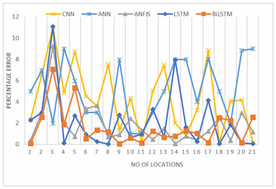
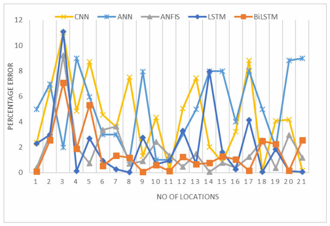
The IEEE 30- and 9-bus systems are simulated in MATLAB to develop fault location models. The various locations on the transmission lines are used to generate faults, and the post-fault current and voltage at one end of the bus in IEEE 9- and IEEE 30-bus systems are measured and used for generating further data in the form of DWT coefficients and all other voltage and current components. To verify the deep learning and machine learning models’ efficiency, RMSE, MAE, and R² are calculated and compared for both the IEEE 9- and 30-bus systems. Equations (20) and (21) give the RMSE and R2, and Equation (22) gives the MAE. The generated results are tabulated in Table 4 and Table 5, which present the predicted locations by the models and their corresponding percentage errors. The reference point for these tables is bus no. 6 in the IEEE 30-bus system and bus no. 7 in the IEEE 9-bus system. The plot is displayed in Figure 13.

Figure 13. Percentage error comparison for deep learning and machine learning models.

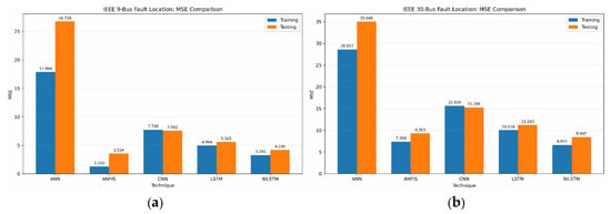
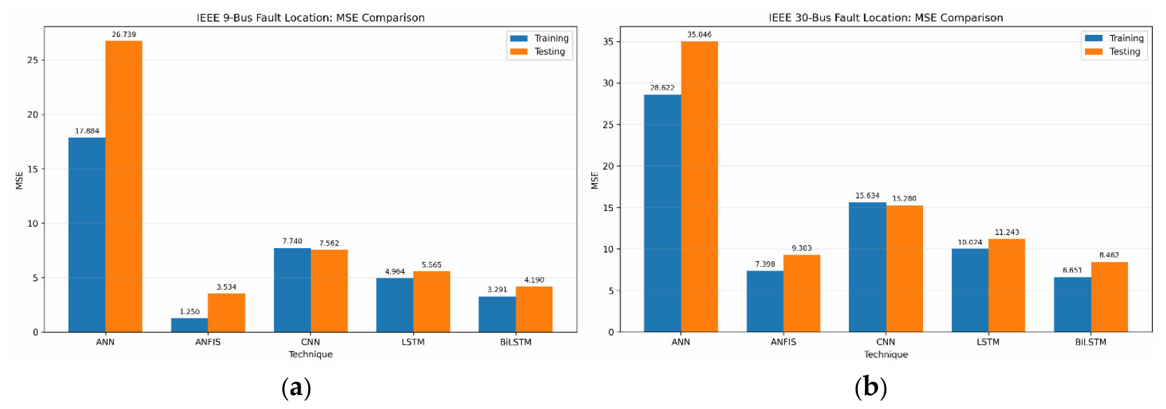
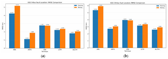
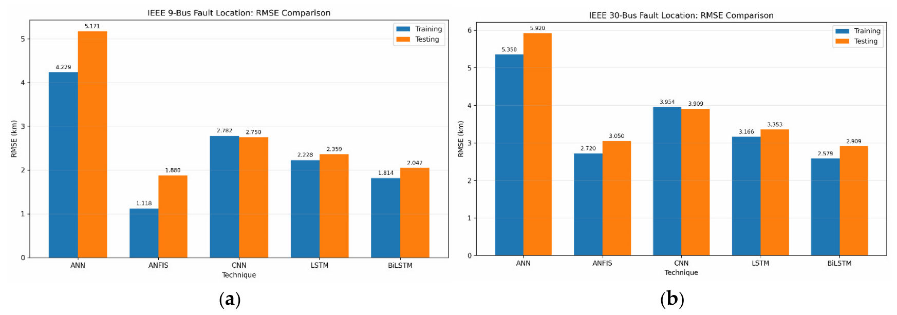
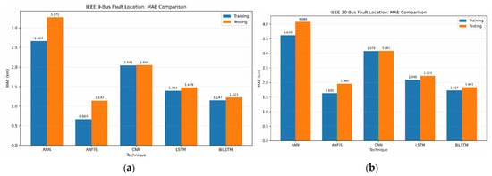
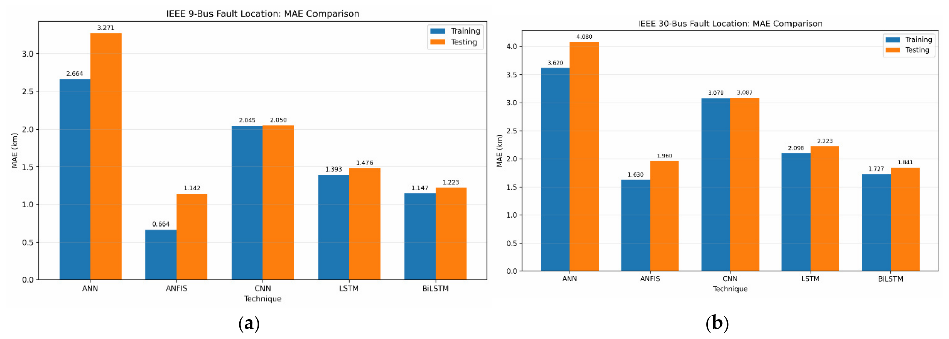
This shows the percentage error for each evaluated model. Further, the results in Table 6 and Table 7 reveal that ANFIS and BiLSTM offer comparatively better performance while achieving the RMSE of 1.880 km and 2.047 km, and MAE of 1.142 km and 1.223 km, respectively, for IEEE 9. In the case of IEEE 30, the performance of ANFIS and BiLSTM is achieved as 3.050 km and 2.909 km, with MAE as 1.960 km and 1.84 km, respectively. In the case of ANFIS, it is able to achieve this due to its capability of learning a relatively compact nonlinear fault-location relationship, using adaptive fuzzy rules. The advantage of BiLSTM’s bidirectional process is apparent in its performance, where the bidirectional recurrent processing was found to capture a greater degree of complex dependencies and scalability. The hybrid nature of both models also contributes to the overall performance compared with the plain models ANN, CNN and LSTM. Thus, it seems that the hybrid architecture for the system is good. Figure 14 shows the MSE comparison for fault location training and testing of ANN, ANFIS, CNN, LSTM and BiLSTM for the IEEE 9- and IEEE 30-bus systems. ANFIS self-based learning and logic decision helped in achieving better performance. In the case of ANN, performance is not better because backpropagation uses a global nonlinear mapping without using an accurate representation of the current condition and the structure’s relationship. Figure 15 represents RMSE for all the models’ training and testing results for fault location in the IEEE-9 and IEEE-30 bus systems, respectively. In the case of CNN and LSTM, there is a deviation between the actual fault location and the predicted fault location. BiLSTM is a deep learning technique as it builds on LSTM and it proceeds with the training and testing process on each signal in both forward and reverse directions. Figure 16 compares the mean absolute error for all the models in the IEEE-9 and IEEE-30 bus systems. ANFIS and BiLSTM demonstrated comparatively strong performance across both the IEEE-9 and IEEE-30 systems under the investigated experimental conditions. The influence of fault position was further investigated by comparing the actual and estimated fault distances at different locations in Table 4 and Table 5. Although prediction errors varied among individual fault positions, no uniform increase in error with increasing fault distance was observed. This suggests that the investigated models were able to identify fault-location characteristics over different portions of the line rather than being restricted to a particular distance range. Variations in error among locations indicate that fault position, together with the corresponding electrical characteristics and network configuration, affects the difficulty of the localization problem. Therefore, the overall RMSE and MAE values should be interpreted together with the location-wise error results. Comparison of results of different fault location models is displayed in Table 8. The results are limited to the data that have been generated online from MATLAB from the point at the bus system; in both systems, the results may vary with different systems.

Table 7. Training and testing results with IEEE 9-bus system.

	Training Results				Testing Results
Models	RMSE (km)	MSE (km2)	MAE (km)	R2	RMSE (km)	MSE (km2)	MAE (km)	R2
CNN	2.782	7.739	2.045	0.991	2.750	7.562	2.050	0.986
LSTM	2.228	4.964	2.228	0.994	2.359	5.564	1.476	0.992
BiLSTM	1.814	3.290	1.147	0.996	2.047	4.190	1.223	0.992
ANFIS	1.118	1.249	0.664	0.998	1.880	3.534	1.142	0.996
ANN	4.229	17.884	2.675	0.977	5.171	26.739	3.271	0.966

Figure 14. (a) MSE comparison for all models in IEEE 9-bus. (b) MSE comparison for all models in IEEE 30-bus fault location.

Figure 15. (a) RMSE comparison for all models in IEEE 9-bus fault location. (b) RMSE comparison for all models in IEEE 30-bus fault location.

Figure 16. (a) MAE comparison for all models in IEEE 9-bus fault location. (b) MAE comparison for all models in IEEE 30-bus fault location.

Table 8. Comparison of results of different fault location models.

Year (Ref)	System	Fault Location Models	Performance (RMSE) km
2025 [55]	Modified IEEE 34-node	Ensemble tree, Decision tree	2.45, 2.70
2026 [56]	400-kV, 300-km, 50-Hz series-compensated transmission line	Artificial Neural Network	3.493
2023 [57]	Transmission-line two-terminal fault location	KNN	2.729
Proposed	IEEE 9, IEEE 30 bus system	BiLSTM, ANFIS	1.841, 1.960

5. Conclusions

This study presents a single-ended fault location framework for transmission lines based on machine learning and deep learning techniques and evaluates its performance on the IEEE 9-bus and IEEE 30-bus systems. Faults were simulated under different fault types, locations, and operating conditions. Post-fault voltage and current signals measured at bus 7 of the IEEE 9-bus system and bus 6 of the IEEE 30-bus system were used to extract electrical and transient features relevant to fault location. A feature-fusion framework was developed by integrating measured voltage and current parameters, transient features obtained through Discrete Wavelet Transform (DWT) analysis, and physically meaningful parameters into a unified input representation. This approach enables the models to exploit complementary steady-state and transient information associated with fault distance. ANN, ANFIS, CNN, LSTM, and BiLSTM models were trained and evaluated using the same feature set and consistent training and testing procedures, allowing their fault-location performance to be compared under comparable conditions. The results demonstrate that the proposed feature-fusion approach provides effective information for accurate fault-location prediction across both test systems. Among the evaluated models, ANFIS and BiLSTM achieved the lowest location errors and demonstrated comparatively better generalization performance, followed by LSTM, CNN, and ANN. The results indicate that the nonlinear learning capability of ANFIS and the sequential learning capability of BiLSTM enable them to effectively capture the complex relationships between the extracted features and fault distance. Overall, the findings demonstrate the potential of combining multi-domain feature information with machine learning and deep learning techniques for accurate single-ended transmission-line fault location under diverse fault conditions.

References

- Leite, D.; Andrade, E.; Rativa, D.; Maciel, A.M. Fault detection and diagnosis in industry 4.0: A review on challenges and opportunities. Sensors 2024, 25, 60. [Google Scholar] [CrossRef] [Scilit]
- Kanwal, S.; Jiriwibhakorn, S. Artificial intelligence based faults identification, classification, and localization techniques in transmission lines—A review. IEEE Lat. Am. Trans. 2023, 21, 1291–1305. [Google Scholar] [CrossRef] [Scilit]
- Kanwal, S.; Jiriwibhakorn, S. Advanced fault detection, classification, and localization in transmission lines: A comparative study of ANFIS, neural networks, and hybrid methods. IEEE Access 2024, 12, 49017–49033. [Google Scholar] [CrossRef] [Scilit]
- Xu, J.; Lu, Y.; Zhao, C.; Liang, J. A model-based DC fault location scheme for multi-terminal MMC-HVDC systems using a simplified transmission line representation. IEEE Trans. Power Deliv. 2020, 35, 386–395. [Google Scholar] [CrossRef] [Scilit]
- Xu, X.; Zhou, F.; Nie, Y.; Xu, W.; Wang, K.; OuYang, J.; Zhou, K.; Chen, S.; Han, Y. Fault detection and location of 35 kV single-ended radial distribution network based on traveling wave detection method. Processes 2023, 11, 2494. [Google Scholar] [CrossRef] [Scilit]
- Li, L.; Yin, Q.; Wang, X.; Wang, H. Defects localization and classification method of power transmission line insulators aerial images based on YOLOv5 EfficientNet and SVM. IEEE Access 2025, 13, 74833–74843. [Google Scholar] [CrossRef] [Scilit]
- Kanwal, S.; Jiriwibhakorn, S. Fault detection in transmission lines using CNN. In Proceedings of the 2024 16th International Conference on Information Technology and Electrical Engineering (ICITEE), Bali, Indonesia, 23–25 October 2024; pp. 24–29. [Google Scholar] [CrossRef] [Scilit]
- Jiriwibhakorn, S.; Kanwal, S. Time series-based fault detection and classification in IEEE 9-bus transmission lines using deep learning. IEEE Access 2025, 13, 118135–118146. [Google Scholar] [CrossRef] [Scilit]
- Arpanahi, M.K.; Fini, M.H.; Nateghi, A. A novel single-end fault location method for double-circuit transmission lines. Int. J. Electr. Power Energy Syst. 2024, 158, 109984. [Google Scholar] [CrossRef] [Scilit]
- Banerjee, S.; Bhowmik, P.S.; Bohre, A.K. Detection and location of fault in microgrid using discrete wavelet transform based technique. In Proceedings of the 2022 IEEE 6th International Conference on Condition Assessment Techniques in Electrical Systems (CATCON), Durgapur, India, 17–19 December 2022; pp. 417–421. [Google Scholar] [CrossRef] [Scilit]
- Mosavi, M.R.; Tabatabaei, A. Traveling-wave fault location techniques in power system based on wavelet analysis and neural network using GPS timing. Wirel. Pers. Commun. 2016, 86, 835–850. [Google Scholar] [CrossRef] [Scilit]
- Yang, K.; Xue, L.; Zhang, W.; Sun, Y. Fault location method based on CNN-BiLSTM-Attention for locating single-phase ground fault in active distribution. In Proceedings of the IECON 2024—50th Annual Conference of the IEEE Industrial Electronics Society, Chicago, IL, USA, 3–6 November 2024; pp. 1–6. [Google Scholar] [CrossRef] [Scilit]
- Wan, W.; Qin, Z.; Deng, M.; Liu, Y. Traveling wave network location method based on adaptive waveform similarity. Heliyon 2024, 10, e37576. [Google Scholar] [CrossRef] [Scilit]
- Zeng, R.; Zhang, L.; Wu, Q.-H. Fault location scheme for multi-terminal transmission line based on frequency-dependent traveling wave velocity and distance matrix. IEEE Trans. Power Deliv. 2023, 38, 3980–3990. [Google Scholar] [CrossRef] [Scilit]
- Livani, H.; Evrenosoglu, C.Y. A machine learning and wavelet-based fault location method for hybrid transmission lines. IEEE Trans. Smart Grid 2014, 5, 51–59. [Google Scholar] [CrossRef] [Scilit]
- Wu, K.; Zhu, L.; Shi, W.; Wang, W.; Wu, J. Self-Attention Memory-Augmented Wavelet-CNN for anomaly detection. IEEE Trans. Circuits Syst. Video Technol. 2023, 33, 1374–1385. [Google Scholar] [CrossRef] [Scilit]
- Anderson, P.; Fouad, A. Power System Control and Stability, 2nd ed.; Wiley: New Delhi, India, 2003. [Google Scholar]
- Sauer, P.; Pai, M.A.; Chow, J.H. Power System Dynamics and Stability, 2nd ed.; Wiley: Hoboken, NJ, USA, 2017. [Google Scholar]
- Obi, O.E.; Ezechukwu, O.A.; Ezema, C.N. An extended ANN-based high-speed accurate transmission line fault location for double phase-to-earth fault on non-direct-ground. Int. J. Eng. Sci. Technol. 2017, 1, 1–7. [Google Scholar] [CrossRef] [Scilit]
- Elkheir, E.S.I.A.; Abd-Allah, M.A.; Hussien, S.A.; Omar, A.I. Real-time microgrid fault management: Leveraging hybrid deep learning for superior detection and classification performance. IEEE Access 2026, 14, 9606–9623. [Google Scholar] [CrossRef] [Scilit]
- Illinois Center for a Smarter Electric Grid (ICSEG). IEEE 30-Bus System. illinois.edu. Available online: https://icseg.iti.illinois.edu/ieee-30-bus-system/ (accessed on 1 October 2026).
- MATLAB, Version 9.7.0 (R2019b); The MathWorks, Inc.: Natick, MA, USA, 2022.
- PSCAD. IEEE 09 Bus System; PSCAD Knowledge Base; Manitoba Hydro International Ltd. Available online: https://www.pscad.com/knowledge-base/article/25 (accessed on 1 October 2026).
- PSCAD. IEEE 30 Bus System; PSCAD Knowledge Base; Manitoba Hydro International Ltd. Available online: https://www.pscad.com/knowledge-base/article/27 (accessed on 1 October 2026).
- Mohamed, S.A.; Anwer, N.; Mahmoud, M.M. Solving optimal power flow problem for IEEE-30 bus system using a developed particle swarm optimization method towards fuel cost minimization. Int. J. Model. Simul. 2025, 45, 307–320. [Google Scholar] [CrossRef] [Scilit]
- Lotfi-fard, S.; Faiz, J.; Iravani, R. Improved overcurrent protection using symmetrical components. IEEE Trans. Power Deliv. 2007, 22, 843–850. [Google Scholar] [CrossRef] [Scilit]
- Magnago, F.H.; Abur, A. Fault location using wavelets. IEEE Trans. Power Deliv. 1998, 13, 1475–1480. [Google Scholar] [CrossRef] [Scilit]
- Salehi, D.; Vafamand, N.; Soltani, S.; Kamwa, I.; Rabiee, A. Wavelet–deep learning framework for high-resolution fault detection, classification, and localization in WMU-enabled distribution systems. Smart Cities 2026, 9, 70. [Google Scholar] [CrossRef] [Scilit]
- Wang, M.-H.; Lu, S.-D.; Liao, R.-M. Fault diagnosis for power cables based on convolutional neural network with chaotic system and Discrete Wavelet Transform. IEEE Trans. Power Deliv. 2022, 37, 582–590. [Google Scholar] [CrossRef] [Scilit]
- Deng, F.; Zhong, Y.; Zeng, Z.; Zu, Y.; Zhang, Z.; Huang, Y.; Feng, S.; Zeng, X. A single-ended fault location method for transmission line based on full waveform features extractions of traveling waves. IEEE Trans. Power Deliv. 2023, 38, 2585–2595. [Google Scholar] [CrossRef] [Scilit]
- Zhang, M.; Gao, Q.; Liu, B.; Zhang, C.; Zhou, G. A method based on CNN–BiLSTM–Attention for wind farm line fault distance prediction. Energies 2025, 18, 3703. [Google Scholar] [CrossRef] [Scilit]
- Krizhevsky, A.; Sutskever, I.; Hinton, G.E. ImageNet classification with deep convolutional neural networks. Adv. Neural Inf. Process. Syst. 2012, 25, 1097–1105. [Google Scholar]
- Arumuga, M.; Reddy, M.J.B. Distance protection methodology for detection of faulted phase and fault along with power swing using apparent impedance. IEEE Access 2022, 10, 43583–43597. [Google Scholar] [CrossRef] [Scilit]
- Chen, Z.; Cai, S.; Meliopoulos, A.P.S. A real-time deep learning-based fault diagnosis framework in power distribution system with PVs. In Proceedings of the 2024 IEEE Power & Energy Society Innovative Smart Grid Technologies Conference (ISGT), Washington, DC, USA, 19–22 February 2024; pp. 1–5. [Google Scholar] [CrossRef] [Scilit]
- Wang, X.; Zhou, P.; Peng, X.; Wu, Z.; Yuan, H. Fault location of transmission line based on CNN-LSTM double-ended combined model. Energy Rep. 2022, 8, 781–791. [Google Scholar] [CrossRef] [Scilit]
- Shrestha, R.; Chamana, M.; Mohammadpourfard, M.; Souto, L.; Bayne, S. Fault detection isolation and localization (FDIL) scheme: A robust ML framework with novel architecture for fault localization. IEEE Access 2025, 13, 172371–172383. [Google Scholar] [CrossRef] [Scilit]
- Ioffe, S. Batch renormalization: Towards reducing minibatch dependence in batch-normalized models. Adv. Neural Inf. Process. Syst. 2017, 30, 1945–1953. [Google Scholar]
- Glorot, X.; Bordes, A.; Bengio, Y. Deep sparse rectifier neural networks. In Proceedings of the Fourteenth International Conference on Artificial Intelligence and Statistics (AISTATS), Fort Lauderdale, FL, USA, 11–13 April 2011; pp. 315–323. [Google Scholar]
- Minh, N.Q.; Khiem, N.T.; Giang, V.H. Fault classification and localization in power transmission line based on machine learning and combined CNN-LSTM models. Energy Rep. 2024, 12, 5610–5622. [Google Scholar] [CrossRef] [Scilit]
- IEEE Standard PC37.114/D8; IEEE Guide for Determining Fault Location on AC Transmission and Distribution Lines. IEEE: Piscataway, NJ, USA, 2014; pp. 1–72.
- Bock, S.; Goppold, J.; Weiß, M. An improvement of the convergence proof of the ADAM-Optimizer. arXiv 2018, arXiv:1804.10587. [Google Scholar]
- Ye, X.; Gao, L.; Li, X.; Wen, L. A new hyper-parameter optimization method for machine learning in fault classification. Appl. Intell. 2023, 53, 14182–14200. [Google Scholar] [CrossRef] [Scilit]
- LeCun, Y.; Bengio, Y.; Hinton, G. Deep learning. Nature 2015, 521, 436–444. [Google Scholar] [CrossRef] [Scilit]
- Hochreiter, S.; Schmidhuber, J. Long short-term memory. Neural Comput. 1997, 15, 1735–1780. [Google Scholar] [CrossRef] [Scilit]
- Khodayar, M.; Liu, G.; Wang, J.; Khodayar, M.E. Deep learning in power systems research: A review. CSEE J. Power Energy Syst. 2020, 7, 209–220. [Google Scholar] [CrossRef] [Scilit]
- Guo, M.F.; Zeng, X.D.; Chen, D.Y.; Yang, N.C. Deep-learning-based earth fault detection using continuous wavelet transform and convolutional neural network in resonant grounding distribution systems. IEEE Sens. J. 2018, 18, 1291–1300. [Google Scholar] [CrossRef] [Scilit]
- Moradzadeh, A.; Teimourzadeh, H.; Mohammadi-Ivatloo, B.; Pourhossein, K. Hybrid CNN-LSTM approaches for identification of type and locations of transmission line faults. Int. J. Electr. Power Energy Syst. 2022, 135, 107563. [Google Scholar] [CrossRef] [Scilit]
- Al-Malah, K.I.M. Machine and Deep Learning Using MATLAB: Algorithms and Tools for Scientists and Engineers; John Wiley & Sons: Hoboken, NJ, USA, 2023. [Google Scholar]
- Wang, Q.; Liang, X.; Qin, S. Research on power quality disturbance analysis and identification based on LSTM. Energy Rep. 2022, 8, 709–718. [Google Scholar] [CrossRef] [Scilit]
- Zhao, H.; Sun, S.; Jin, B. Sequential fault diagnosis based on LSTM neural network. IEEE Access 2018, 6, 12929–12939. [Google Scholar] [CrossRef] [Scilit]
- Li, Z.; Liu, F.; Yang, W.; Peng, S.; Zhou, J. A survey of convolutional neural networks: Analysis, applications, and prospects. IEEE Trans. Neural Netw. Learn. Syst. 2022, 33, 6999–7019. [Google Scholar] [CrossRef] [Scilit]
- Roy, B.; Adhikari, S.; Datta, S.; Devi, K.J.; Devi, A.D.; Alsaif, F.; Alsulamy, S.; Ustun, T.S. Deep learning based relay for online fault detection, classification, and fault location in a grid-connected microgrid. IEEE Access 2023, 11, 62674–62696. [Google Scholar] [CrossRef] [Scilit]
- Jang, J.-S.R. ANFIS: Adaptive-network-based fuzzy inference system. IEEE Trans. Syst. Man Cybern. 1993, 23, 665–685. [Google Scholar] [CrossRef] [Scilit]
- Reddy, M.J.B.; Mohanta, D.K. Performance evaluation of an adaptive-network-based fuzzy inference system approach for location of faults on transmission lines using Monte Carlo simulation. IEEE Trans. Fuzzy Syst. 2008, 16, 909–919. [Google Scholar] [CrossRef] [Scilit]
- Lopes, G.N.; Barbalho, P.I.N.; Vieira, J.C.M.; Coury, D.V. High Impedance Fault Location in Distribution Systems: A Novel Approach With Enhanced Metrics and Intelligent Algorithms. IEEE Access 2025, 13, 108466–108480. [Google Scholar] [CrossRef] [Scilit]
- Moparthi, J.R.; Bhukya, K.N.; Kethavath, R.N.; Kolhe, M.L.; Borut, J. Intelligent Ensemble Learning-Based Fault Diagnosis, Location, and Protection of Series-Compensated Transmission Lines for Smart Power Grid Applications. Energies 2026, 19, 3765. [Google Scholar] [CrossRef] [Scilit]
- Su, C.; Yang, Q.; Wu, X.; Lai, C.S.; Lai, L.L. A Two-Terminal Fault Location Fusion Model of Transmission Line Based on CNN-Multi-Head-LSTM with an Attention Module. Energies 2023, 16, 1827. [Google Scholar] [CrossRef] [Scilit]
Disclaimer/Publisher’s Note: The statements, opinions and data contained in all publications are solely those of the individual author(s) and contributor(s) and not of MDPI and/or the editor(s). MDPI and/or the editor(s) disclaim responsibility for any injury to people or property resulting from any ideas, methods, instructions or products referred to in the content. |
© 2026 by the authors. Licensee MDPI, Basel, Switzerland. This article is an open access article distributed under the terms and conditions of the Creative Commons Attribution (CC BY) license.