A Three-Level Global-Local Coupling Strategy with Non-Matching Interfaces for Crack Propagation Analysis in Beam-Solid Structures

Abstract

Global-local non-intrusive coupling is a well-established strategy for the analysis of structures with localised non-linear behaviour, but its practical applicability is limited by the requirement that the local patch coincides with a node of the global mesh. This work proposes a three-level non-intrusive global-local coupling strategy in which an intermediate 1D beam model is inserted between the global and the local domains, restoring full freedom in the placement of the local patch without modifying the global model. The formulation transfers displacements and reactions between two non-coincident interfaces through explicit projection operators, and the additional level introduces only three beam elements and four nodes per coupling region. The methodology is validated on a cantilever beam (linear, notched and crack-propagation variants) and on a three-storey framed structure with X-FEM crack propagation, against a monolithic 3D reference and against the standard matching-interface global-local method. For the framed structure, the non-matching scheme reduces the total degrees of freedom by 97.46% with respect to the monolithic solution and cuts the computation time by 68.19%, compared to 53.86% for the matching-interface version. Displacement errors remain below 10% and iteration counts drop by up to one third with respect to the matching scheme. The proposed formulation is therefore accurate, computationally efficient, and geometrically flexible in scenarios where the global model cannot be modified.

1. Introduction

Mechanical simulation of structures with localised non-linear behaviour: plasticity [1], contact [2] and crack propagation, is computationally demanding because of the iterative nature of the solvers [3] and the need to discretise the entire structure at the resolution required by the non-linear region [4,5]. Several families of strategies have been developed to alleviate this cost.

Domain decomposition methods [6,7,8,9,10] partition an a-priori monolithic model into subdomains coupled through Lagrange multipliers or balanced operators, and rely on parallel computing for efficiency. They assume that the complete model is available, and that all subdomains are discretised at compatible resolutions. Submodeling, sometimes referred to as top-down or descendant analysis [11,12], extracts a refined local model from the boundary conditions delivered by a coarser global model, but does not feed the non-linear effect back into the global solution, so any global redistribution of stresses caused by local damage is lost.

Non-intrusive global-local coupling [13,14,15,16] removes both restrictions. The global model, typically coarse and linear, is solved iteratively with a small non-linear patch by means of a primal-dual exchange of displacements and reaction forces at a common interface $\Gamma$. The method has been successfully applied to plasticity, phase-field damage and crack propagation [17,18,19,20,21,22,23], and converges to the solution of a fully refined monolithic problem without modifying the global model. The convergence rate, however, depends on the contrast between the local and the global stiffness and on the size of the local patch [24,25] and several relaxation and acceleration techniques have been used to increase the convergence rate [14,26,27,28,29].

Mixed-dimensional coupling has emerged as another avenue for combining computationally efficient reduced structural models with detailed 3D continuum descriptions. Mortar-type embedding of one-dimensional beams within 3D solid volumes is one example of this [30], as are the non-intrusive coupling of shell and solid models across three scales of analysis [31] and the coupling of full and reduced finite elements with non-matching meshes in mixed-dimensional configurations [32]. The issue of non-conforming meshes has also been addressed more generally, without resorting to a global-local iterative scheme: enriched interface formulation and mortar-based techniques allow for the enforcement of kinematic compatibility and the consistent transfer of interface forces between independently discretised regions [33,34,35].

A separate difficulty appears when the global model is a 1D beam representation of a civil structure and the local model is a fully 3D continuum [36,37]. The size of the local model that guarantees convergence (determined for instance by the discriminant criterion of [25]) does not generally coincide with the position of any node of the existing 1D mesh. Forcing coincidence either modifies the global model (and breaks non-intrusiveness) or restricts the local patch to a length that does not match the requirement, reducing the practical applicability of the method.

This work proposes a three-level nonm-intrusive global-local strategy in which an intermediate 1D beam model is inserted between the global and the local domains. The intermediate level inherits the cross-section and material of the global beam, includes the interface $\gamma$ matching the local 3D mesh, and transmits displacements and reactions between two non-coincident interfaces ($\Gamma$ between global and intermediate, $\gamma$ between intermediate and local). The cost of the additional level is negligible (three elements, four nodes per coupling region) but it restores full freedom in the choice of the local patch length without modifying the global model. The methodology is validated against a monolithic 3D reference and against the standard matching-interface global-local method on a cantilever beam and on a multi-storey framed structure, including X-FEM crack propagation. The formulation is stated in terms of explicit projection operators between the one-dimensional and three-dimensional kinematic representations, and the compatibility conditions on the two non-coincident interfaces are expressed as algebraic constraints on the coupled system.

The remainder of the paper is organised as follows. Section 2 presents the three-level formulation, including the projection operators that map kinematic quantities between the 1D and the 3D representations, and the cases of study used for validation. Section 3 reports the displacement, stress and crack-front results of the cantilever beam and of the framed structure, and quantifies the iteration and CPU savings obtained against the matching-interface method. Section 4 discusses the limitations and outlook of the approach.

2. Methodology

2.1. Three-Level Non-Intrusive Global-Local Formulation with Non-Matching Interfaces

Performing a 1D-to-3D global/local analysis consists of separating the real mechanical problem into a 1D global problem and a 3D local problem, capturing the nonlinearity.

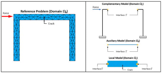
Considering that the structure occupies a domain ${\mathsf{\Omega }}_R$ (Figure 1), this domain is partitioned into two subdomains coupled through a one-dimensional interface $\Gamma$: the complementary domain ${\mathsf{\Omega }}_C$ and the local domain ${\mathsf{\Omega }}_L$, the latter possibly containing non-linearities. In the non-intrusive setting, the global model is not restricted to ${\mathsf{\Omega }}_C$ but is defined over the whole domain ${\mathsf{\Omega }}_G={\mathsf{\Omega }}_C\cup {\mathsf{\Omega }}_A$, where ${\mathsf{\Omega }}_A$ is an auxiliary subdomain that overlaps with ${\mathsf{\Omega }}_L$ and shares the linear behaviour of ${\mathsf{\Omega }}_C$. This overlap enables the primal-dual exchange of displacements and reactions on the shared interface $\Gamma$ without requiring any modification of the global mesh.

Figure 1. Real mechanical problem and its global/local decomposition for a framed structure.

In the matching-interface formulation of [36], the position of $\Gamma$ in the global model coincides with the position of $\Gamma$ in the local model. The proposed three-level extension introduces an intermediate domain ${\mathsf{\Omega }}_I$ that decouples this position constraint.

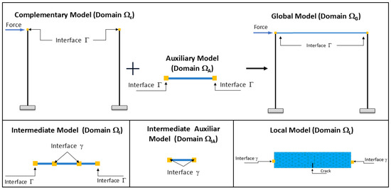
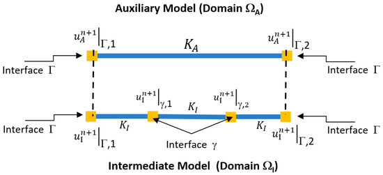
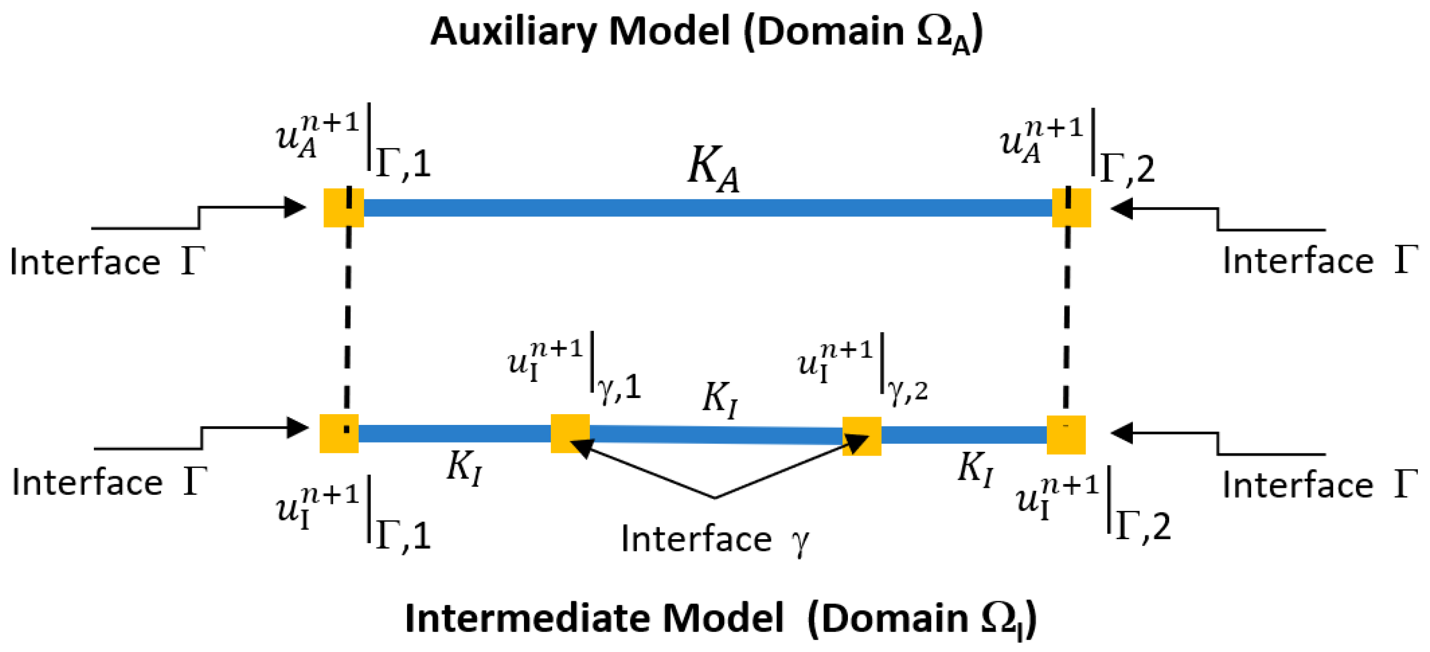
In this document, we studied the case when, unlike Figure 1, the interface $\Gamma$ does not match in the models. Consequently, a new intermediate 1D beam-type model is introduced with the same properties as the auxiliary part. Figure 2 illustrates the five domains involved in the formulation and their interface regions.

Figure 2. Domains of the three-level non-intrusive global/local methodology.

Each of the models is discretised as follows:

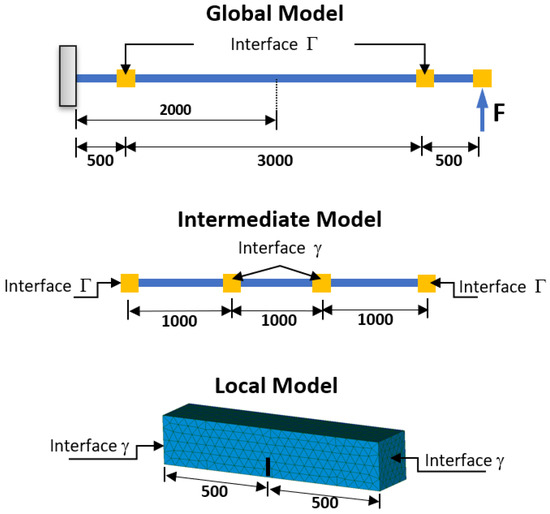
• Global Model, $\left({\mathsf{\Omega }}_G\right)$: 3 Linear Beam elements, with 4 nodes with 6 degrees of freedom each. 2 nodes are clampled, and the other 2 are connected to the Interface $\Gamma$.
• Intermediate Model, $\left({\mathsf{\Omega }}_I\right)$: 3 Linear Beam elements, with 4 nodes with 6 degrees of freedom each. The external nodes are connected to the Interface $\Gamma$, while the internal nodes are connected to the interface $\gamma$.
• Auxiliary Model, $\left({\mathsf{\Omega }}_A\right)$: 1 Linear Beam elements, with 2 nodes with 6 degrees of freedom each. The nodes are connected to the Interface $\Gamma$.
• Local Model, $\left({\mathsf{\Omega }}_L\right)$: Non-Linear 3D model of the local subdomain, connected to the interface $\gamma$.
• Intermediate Auxiliary Model, $\left({\mathsf{\Omega }}_{IA}\right)$: 1 Linear Beam elements, with 2 nodes with 6 degrees of freedom each. The nodes are connected to the Interface $\gamma$.

By including the intermediate model, the problem is solved by the iterative procedure described in detail in the steps that follow.

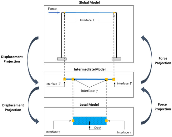
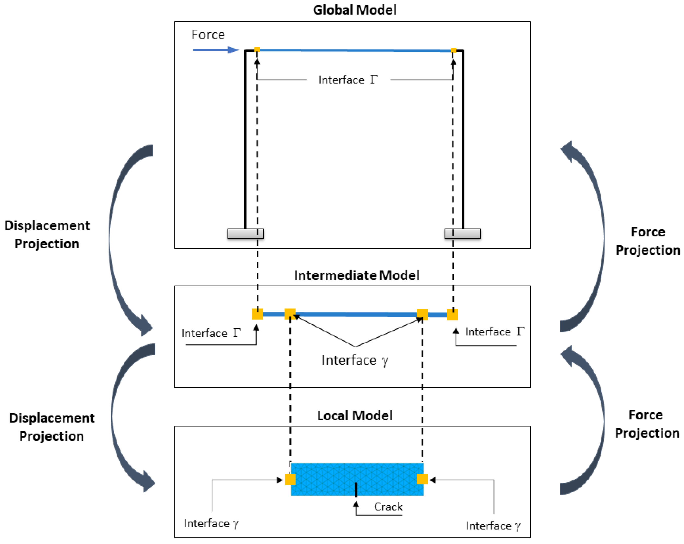
Figure 3 illustrates the methodology in a simplified manner, showing how displacements and rotations are projected from the global model to the local model, while forces are projected from the local model back to the global model.

Figure 3. Schematic of the three-level non-intrusive global/local methodology.

With the inclusion of this new interface zone, the resolution process consists of the following steps:

• Solve the global model to obtain the global displacements and rotations $u_G^{n+1}$:

  $$K_G{u}_G^{n+1}=f_d^G+C_G^T{P}^n$$

  (1)

  where $K_G$ is the stiffness matrix of the global model, $f_d^G$ is the vector of external forces, $C_G$ is a coupling operator for the global problem that relates the degrees of freedom of the interface to the degrees of freedom of the entire domain, enabling the application of correction forces at the nodes of the $\Gamma$ interface ($C_G$ has dimension $12\times 6n_G$, where $n_G$ is the number of nodes of the global model and 12 corresponds to the six degrees of freedom of each of the two nodes of $\Gamma$), and $P^n$ represents the correction forces from the previous iteration. In the first iteration, $P^n$ is a zero vector. The vector $P^n$, as well as all quantities defined at the two nodes of $\Gamma$ or $\gamma$ in the following steps (such as $u_A$, ${\lambda }_A$, ${\lambda }_{IA}$, ${\lambda }_{LI}$ and $P_I$), has dimension 12.
  Then, the displacements and rotations of the auxiliary model $u_A^{n+1}$ at the $\Gamma$ interface are calculated using the global displacements $u_G^{n+1}$ via:

  $$u_A^{n+1}=C_G{u}_G^{n+1}=u_G^{n+1}{|}_{\Gamma }$$

  (2)
• Solve the auxiliary problem by imposing displacements and rotations $u_A^{n+1}$ to calculate the reaction forces ${\lambda }_A^{n+1}$ at the $\Gamma$ interface:

  $${\lambda }_A^{n+1}=K_A{u}_A^{n+1}-f_d^A$$

  (3)

  where $K_A$ is the stiffness matrix of the auxiliary model and ${\lambda }_A^{n+1}$ represents the reaction forces at the interface $\Gamma$. The term $f_d^A$ is the equivalent nodal load vector (consistent fixed-end forces) of any distributed load acting along the physical segment represented by ${\mathsf{\Omega }}_A$; since this segment is an actual portion of the original structure, this term must be retained to keep ${\lambda }_A^{n+1}$ consistent with the loading already embedded in $f_d^G$.
• Relate the degrees of freedom of the auxiliary model to the nodes of the $\Gamma$ interface in the intermediate model:

  $$C_I{u}_I^{n+1}=u_I^{n+1}{|}_{\Gamma }=u_A^{n+1}$$

  (4)

  where $C_I$ is a coupling operator that relates the degrees of freedom of the interface to the degrees of freedom of the intermediate domain ($12\times 6n_I$, $n_I$ being the number of nodes of the meshed intermediate model), since the intermediate model has four interface nodes, while the auxiliary model only has two nodes. Figure 4 graphically illustrates the relationship between displacements and rotations from the auxiliary model to the intermediate model, where the auxiliary displacements and rotations vector is $u_A^{n+1}=(u_A^{n+1}{|}_{\Gamma ,1},u_A^{n+1}{|}_{\Gamma ,2})$, and the intermediate model vector at its interface nodes is $u_I^{n+1}=(u_I^{n+1}{|}_{\Gamma ,1},u_I^{n+1}{|}_{\gamma ,1},u_I^{n+1}{|}_{\gamma ,2},u_I^{n+1}{|}_{\Gamma ,2})$.
  

  Figure 4. Projection of displacements from the auxiliary model to the intermediate model at the $\Gamma$ interface.
• Impose the displacements and rotations on the intermediate model to calculate the displacements and rotations $u_I^{n+1}{|}_{\gamma }$ at the intermediate model’s $\gamma$ interface, with $u_I^{n+1}{|}_{\gamma }=(u_I^{n+1}{|}_{\gamma ,1},u_I^{n+1}{|}_{\gamma ,2})$ and $u_I^{n+1}{|}_{\Gamma }=(u_I^{n+1}{|}_{\Gamma ,1},u_I^{n+1}{|}_{\Gamma ,2})$, resulting in:

  $$\left[\begin{array}{cc}{K}_I^{\Gamma \Gamma }& K_I^{\Gamma \gamma }\\ K_I^{\gamma \Gamma }& K_I^{\gamma \gamma }\end{array}\right]\left[\begin{array}{c}{u}_I^{n+1}{|}_{\Gamma }\\ u_I^{n+1}{|}_{\gamma }\end{array}\right]=\left[\begin{array}{c}{f}_d^{I\Gamma }\\ f_d^{I\gamma }\end{array}\right]$$

  (5)

  where $K_I$ terms represent the stiffness matrix of the intermediate model at the $\Gamma$ and $\gamma$ interfaces, and $f_d^{I\Gamma }$ and $f_d^{I\gamma }$ are the external force vectors at these interfaces, respectively. Solving for the displacements and rotations $u_I^{n+1}{|}_{\gamma }$ in Equation (5) yields:

  $$u_I^{n+1}{|}_{\gamma }={\left(K_I^{\gamma \gamma }\right)}^{-1}\left(f_d^{I\gamma }-K_I^{\gamma \Gamma }{u}_I^{n+1}{|}_{\Gamma }\right)$$

  (6)

  where $K_I^{\gamma \gamma }$ corresponds to the condensed stiffness of the intermediate model at interface $\gamma$, and $u_I^{n+1}{|}_{\gamma }$ represents the displacements and rotations obtained at the $\gamma$ interface of the intermediate model, which are subsequently imposed as boundary conditions on the local model in the next step.
• The displacements and rotations $u_I^{n+1}{|}_{\gamma }$ of the intermediate model (1D) are projected onto the interface $\gamma$ of the local model (3D). Here, $u_L^{n+1}$ is the displacement vector for the entire domain ${\mathsf{\Omega }}_L$, while $u_L^{n+1}{|}_{\gamma }$ is the displacement vector of the local model at the interface $\gamma$. This relationship is expressed as:

  $$u_L^{n+1}{|}_{\gamma }=C_L{u}_L^{n+1}={\mathbf{Pr}}_{\mathbf{IL}}\left\{u_I^{n+1}{|}_{\gamma }\right\}$$

  (7)

  where $C_L$ is a coupling operator relating the degrees of freedom of the whole local 3D domain to those of the interface, in the same domain ($3n_{\gamma }\times 3n_L$, where $n_L$ is the number of nodes of the local model and $n_{\gamma }$ the number of its nodes on $\gamma$), and ${\mathbf{Pr}}_{\mathbf{IL}}$ is a projection operator mapping the displacements and rotations of the 1D nodes of $\gamma$ onto the nodes of the 3D interface. Each interface section is treated as a rigid, non-warping plane rotating about its centroid; the displacement imposed on a node of the 3D interface, in terms of the translations and rotations of the corresponding 1D node, is

  $$u=\left\{\begin{array}{c}{u}_x+{\Delta }_x({\theta }_y,{\theta }_z)\\ u_y+{\Delta }_y({\theta }_x,{\theta }_z)\\ u_z+{\Delta }_z({\theta }_x,{\theta }_y)\end{array}\right\}.$$

  (8)

  where each $\Delta$ term is the geometric displacement produced by the corresponding bending or torsional rotation about the section centroid, obtained from kinematic compatibility. A detailed description of the equations used is described in [36].
• The local problem (nonlinear 3D) is solved by imposing the displacements $u_L^{n+1}{|}_{\gamma }$ at the interface $\gamma$ of the local model and calculating the displacements at the internal nodes of the mesh, $u_{Li}^{n+1}$:

  $$\left[\begin{array}{cc}{K}_L^{\gamma \gamma }\left(u^{xFem}\right)& K_L^{\gamma i}\left(u^{xFem}\right)\\ K_L^{i\gamma }\left(u^{xFem}\right)& K_L^{ii}\left(u^{xFem}\right)\end{array}\right]\left[\begin{array}{c}{u}_L^{n+1}{|}_{\gamma }\\ u_{Li}^{n+1}\end{array}\right]=\left[\begin{array}{c}{f}_d^{L\gamma }\\ f_d^{Li}\end{array}\right]$$

  (9)

  where $f_d^{L\gamma }$ and $f_d^{Li}$ represent the equivalent nodal load vectors at the interface $\gamma$ and at the internal mesh nodes, respectively, obtained by integrating the body forces and the surface tractions acting on the local model, excluding the interface $\gamma$, with the shape functions of the 3D elements. The terms $K_L\left(u^{xFem}\right)$ denote the stiffness matrix of the local model, in which $u^{xFem}$ is the X-FEM enriched displacement field that represents the crack discontinuity. Since the local problem is non-linear, $K_L$ depends on $u^{xFem}$ through element weakening, and the system is solved iteratively using X-FEM.
• The reaction forces ${\lambda }_L^{n+1}$ of the local model are calculated, considering $u_L^{n+1}=(u_L^{n+1}{|}_{\gamma },u_{Li}^{n+1})$:

  $${\lambda }_L^{n+1}=K_L\left(u^{xFem}\right)u_L^{n+1}-f_d^L$$

  (10)
• The resultant reaction forces ${\lambda }_{LI}^{n+1}$ at the interface $\gamma$, which will be applied to the intermediate model, are computed as:

  $${\lambda }_{LI}^{n+1}={\mathbf{Pr}}_{\mathbf{LI}}\left\{C_L{\lambda }_L^{n+1}\right\}$$

  (11)

  where ${\mathbf{Pr}}_{\mathbf{LI}}$ is a projection operator mapping forces from the 3D model to the 1D model. The nodal reaction forces at the interface, ${\overrightarrow{f}}_i$, are summed component-wise in x, y and z to obtain the resultant force, and the moment generated by each nodal force about the section centroid is summed to obtain the resultant moment:

  $$\overrightarrow{F}=\sum _i{\overrightarrow{f}}_i,\overrightarrow{M}=\sum _i{\overrightarrow{r}}_i\times {\overrightarrow{f}}_i,$$

  (12)

  where ${\overrightarrow{r}}_i$ is the position vector of node i relative to the section centroid. This operation is computed in Code_Aster with the RESULTANTE/MOMENT/POINT operands of the function POST_RELEVE_T [38].
• The correction forces $P_I^{n+1}$ to be applied to the intermediate model are calculated as:

  $$P_I^{n+1}={\lambda }_{LI}^{n+1}-{\lambda }_{IA}^{n+1}$$

  (13)

  where ${\lambda }_{IA}^{n+1}$ are the reaction forces of the intermediate auxiliary model at the $\gamma$ interface. The subscript $IA$ refers to this model, ${\mathsf{\Omega }}_{IA}$, which plays at $\gamma$ the same role that ${\mathsf{\Omega }}_A$ plays at $\Gamma$: it is the segment of the intermediate model between the two nodes of $\gamma$, i.e., the undamaged 1D counterpart of the local model. This problem is solved, as for the Auxiliary model, for the displacements and rotations obtained at the intermediate model on interface $\gamma$, $u_I^{n+1}{|}_{\gamma }$:

  $${\lambda }_{IA}^{n+1}=K_{IA}{u}_{IA}^{n+1}-f_d^{IA}=K_{IA}{u}_I^{n+1}{|}_{\gamma }-f_d^{IA}$$

  (14)

  where $K_{IA}$ is the stiffness matrix of ${\mathsf{\Omega }}_{IA}$ and $f_d^{IA}$ is its equivalent nodal load vector, which represents in the 1D model the same loads that $f_d^L$ represents in the 3D local model.
• The forces $P_I^{n+1}$ are applied, and the displacements and rotations $u_I^{n+1}{|}_{\Gamma }$ are imposed on the intermediate model to compute the updated displacements and rotations $u_I^{n+1}{|}_{\gamma }$:

  $$\left[\begin{array}{cc}{K}_I^{\Gamma \Gamma }& K_I^{\Gamma \gamma }\\ K_I^{\gamma \Gamma }& K_I^{\gamma \gamma }\end{array}\right]\left[\begin{array}{c}{u}_I^{n+1}{|}_{\Gamma }\\ u_I^{n+1}{|}_{\gamma }\end{array}\right]=\left[\begin{array}{c}{f}_d^{I\Gamma }\\ f_d^{I\gamma }+P_I^{n+1}\end{array}\right]$$

  (15)
• The reaction forces ${\lambda }_I^{n+1}{|}_{\Gamma }$ corresponding to the interface $\Gamma$ of the intermediate model are computed as:

  $${\lambda }_I^{n+1}{|}_{\Gamma }=C_I(K_I{u}_I^{n+1}-f_d^I)$$

  (16)
• The correction forces $P^{n+1}$ at the interface $\Gamma$ to be applied to the global model are calculated as:

  $$P^{n+1}={\lambda }_I^{n+1}{|}_{\Gamma }-{\lambda }_A^{n+1}$$

  (17)
• The residual force $r^{n+1}$ is computed, and the error $\eta$ of the solution at the current iteration is estimated:

  $$r^{n+1}=P^{n+1}-P^n$$

  (18)

  $$\eta ={\displaystyle \frac{\Vert r^{n+1}{\Vert }_2}{\Vert r^0{\Vert }_2}}$$

  (19)
• Finally, an Aitken relaxation technique is applied to improve convergence [14]. The relaxation parameter is set to ${\mu }^{n+1}=1$ in the first two iterations and, from the third iteration onward, is updated from the last two residuals as

  $${\mu }^{n+1}=-{\mu }^n{\displaystyle \frac{{\left(r^n\right)}^T\left(r^{n+1}-r^n\right)}{\Vert r^{n+1}-r^n{\Vert }^2}},$$

  (20)

  resulting in the following correction force:

  $$P^{n+1}={\mu }^{n+1}{P}^{n+1}+(1-{\mu }^{n+1})P^n$$

  (21)

Given that the proposed methodology is an iterative process, the described steps are repeated until the error ($\eta$) falls below a user-defined tolerance. A tolerance of ${10}^{-6}$ is used. The same relaxation scheme and initialisation are used for both the matching and the non-matching interface cases, so that $\mu$ adapts automatically to the stiffness contrast and to the size of the local patch without case-specific tuning.

2.2. Study Cases

2.2.1. Fixed Beam

The case study used to test the methodology with the inclusion of the intermediate model is a cantilever steel beam subjected to a point load at its free end (10 KN), with a length of 4 m. The cross-section of the beam is rectangular with a side length of 200 mm, and the material is steel with an elastic modulus of 200,000 MPa and a Poisson’s ratio of 0.3.

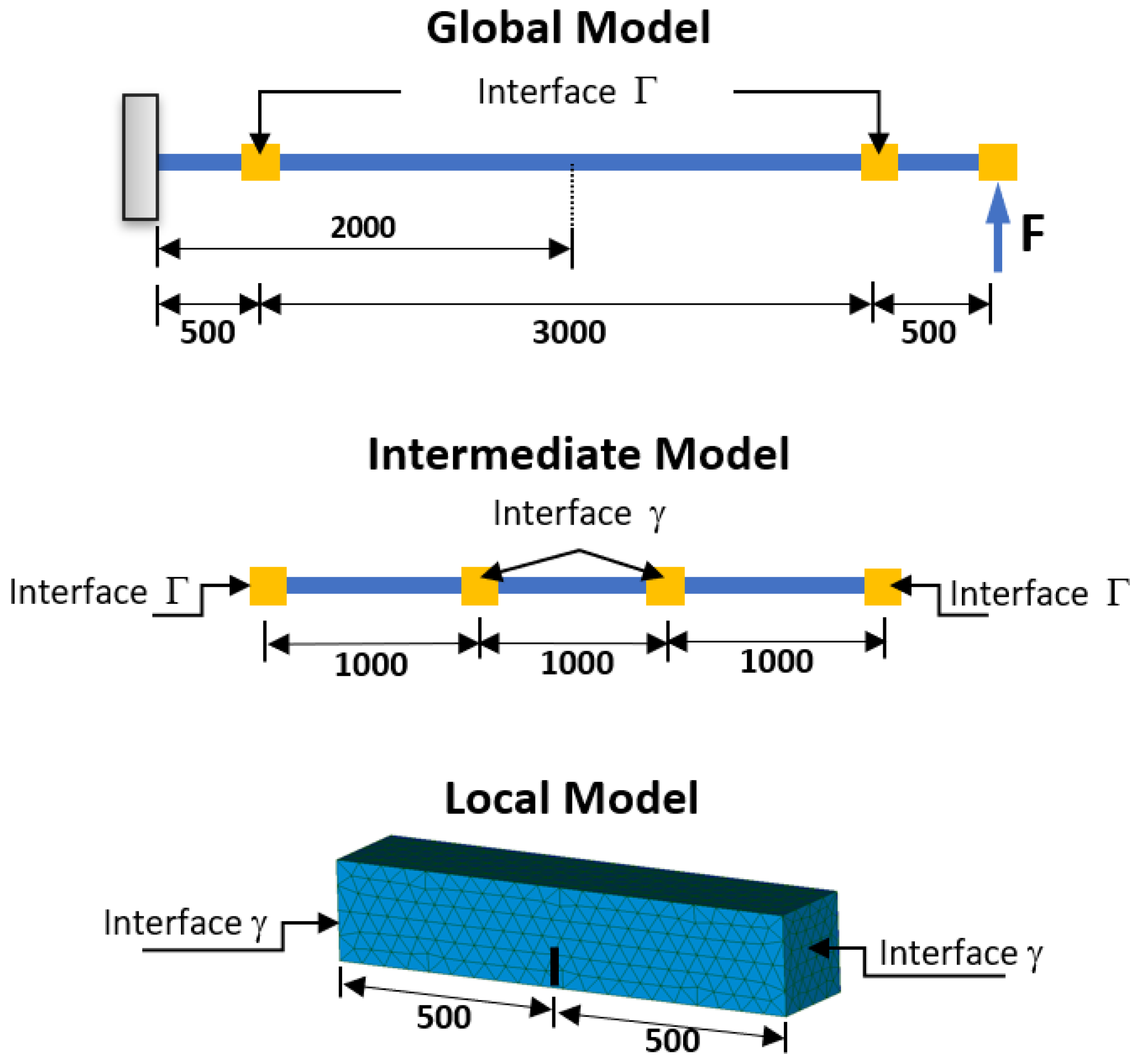
Figure 5 shows the three models into which the structure is discretized and identifies the interfaces of the methodology: $\Gamma$, from which displacements and rotations are extracted from the global model and applied at the $\Gamma$ interface of the intermediate model; and $\gamma$, where displacements obtained from the intermediate model are projected onto the local 3D model.

Figure 5. Cantilever beam case study: 1D global model (top), 1D intermediate model with four nodes and three elements (middle), and 3D local model (bottom).

The analysis considered three case studies:

• Linear problem: It represents a simple base case that allows for validation of the methodology and comparison with traditional analytical and numerical solutions. It facilitates the evaluation of the coupling between different models without the interference of complex geometric effects.
• Linear problem with a notch: It introduces a geometric discontinuity that generates stress concentrations and allows the performance of the method to be evaluated on this type of problem. The notch is assumed to be 50 mm high and 200 mm wide at the center of the beam (x = 2000 mm).
• Nonlinear problem of crack propagation: The ability of the method to model progressive damage and crack propagation within a structure is evaluated. This is a nonlinear problem that requires adequate information transfer between models. Furthermore, this phenomenon has been used in [36] to apply global/local analysis by coupling 1D and 3D beam models with a matching interface. The crack is located at the center of the beam (x = 2000 mm) with a length of 50 mm, and two propagation steps were considered.

The global and intermediate models are defined using Bernoulli-Euler beam theory and exhibit linear behavior, considering six degrees of freedom ($u_x$, $u_y$, $u_z$, ${\theta }_x$, ${\theta }_y$, ${\theta }_z$). For the local model, 3D tetrahedral elements with linear shape functions are used, considering three degrees of freedom ($u_x$, $u_y$, $u_z$), as in [36]. All models are solved using the Code_Aster software.

2.2.2. Framed Structure

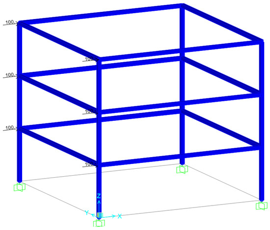
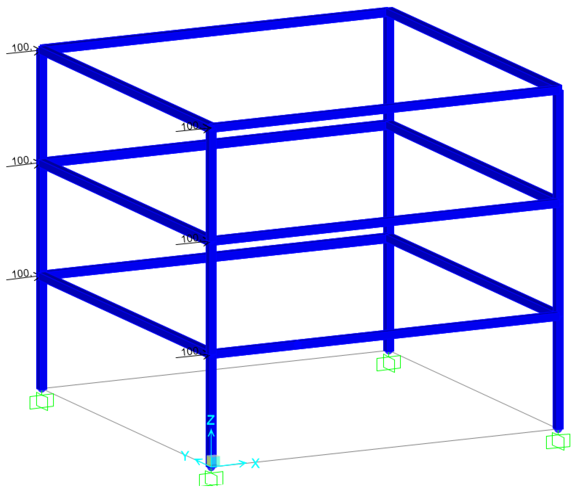
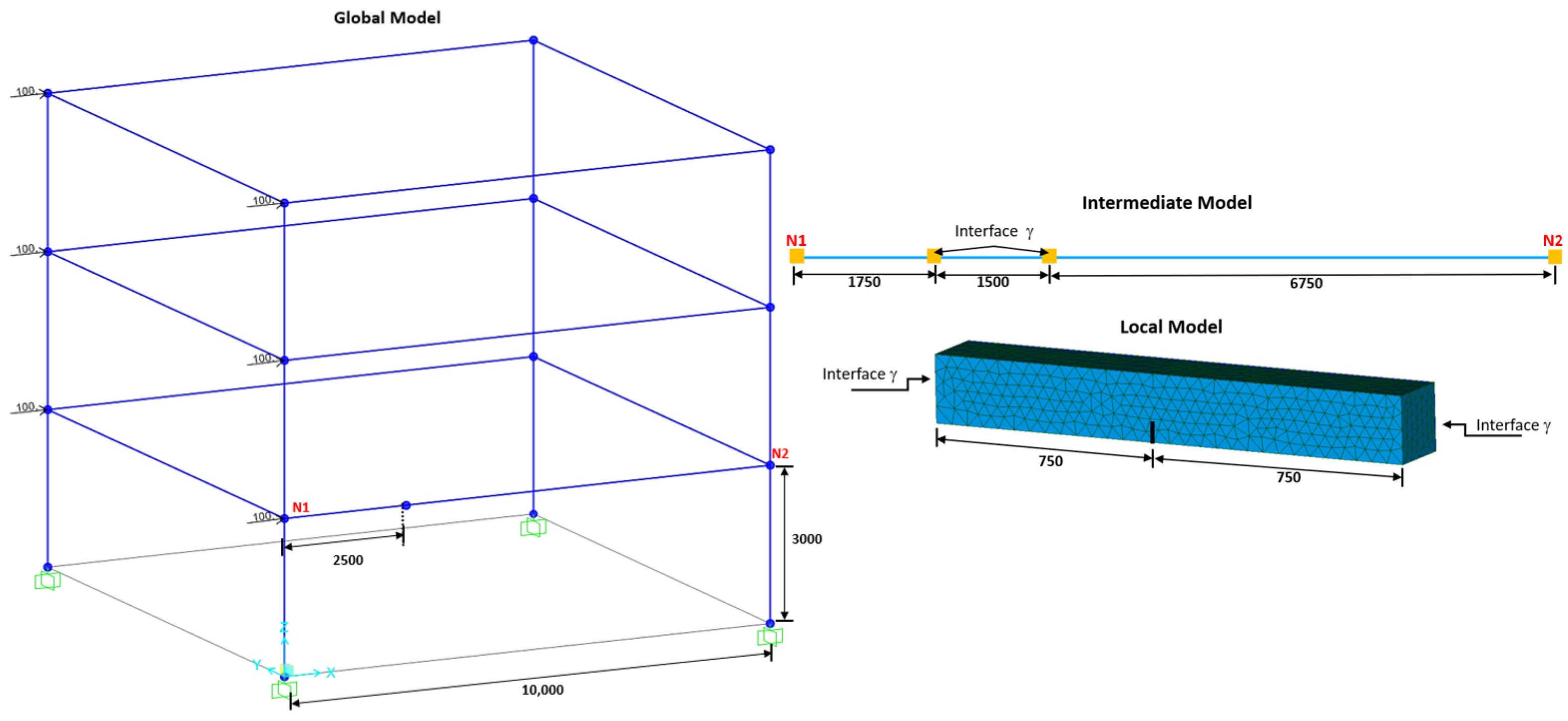
The second case study to test the proposed methodology is a three-story framed structure with a rectangular section subjected to a uniform lateral load pattern, as shown in Figure 6. The structure has a height of 3 m per story and a span of 10 m, while the cross-sections of the columns and beams are rectangular with a side length of 200 mm. The material considered is steel with an elastic modulus of 200,000 MPa and a Poisson’s ratio of 0.3. Horizontal static point loads of 100 kN are applied at the beam-column joints of each of the three story levels shown in Figure 6 (two joints per story, six load points in total). In both study cases, the loads are point loads applied outside the coupling region, so the equivalent nodal load vectors $f_d^A$, $f_d^I$, $f_d^{IA}$ and $f_d^L$ are zero; they are retained in the formulation for generality.

Figure 6. Framed structure under lateral loading.

Figure 7 presents the three models in which the structure is discretized. The nodes numbered N1 and N2 in the global model correspond to the interface $\Gamma$ to couple the global and intermediate models. Meanwhile, in the intermediate and local models, the $\gamma$ interface is shown to couple the intermediate and local models.

Figure 7. Discretization of the framed structure into global, intermediate and local models.

In this case, the ability of the proposed methodology to model damage induced by crack propagation and its effect on a structure specifically used in buildings is evaluated. As in the case of the beam (Section 2.2.1), this phenomenon is studied considering a coincident interface between the global and local models. The crack is located at x = 2500 on the first story.

Crack propagation in both case studies is implemented in Code_Aster: the crack is initialised with DEFI_FISS_XFEM, the energy-release rate and stress-intensity factors are computed with CALC_K_G, and the propagation of the front over a prescribed number of steps is driven by PROPA_FISS. In the local 3D model, the crack is represented as an X-FEM enrichment; the global and intermediate 1D models are unaffected by the crack representation.

3. Results Using Code_Aster with the Proposed Methodology

3.1. Validation of the Methodology Using the Fixed-Beam Results

The validation of the methodology is performed by comparing the displacements obtained from the non-intrusive non-matching global/local analysis with those from a monolithic model and the non-intrusive matching global/local analysis. It is worth mentioning that the analysis of the monolithic model and the matching non-intrusive model considers the same properties as the case studies presented in Section 2.2.1.

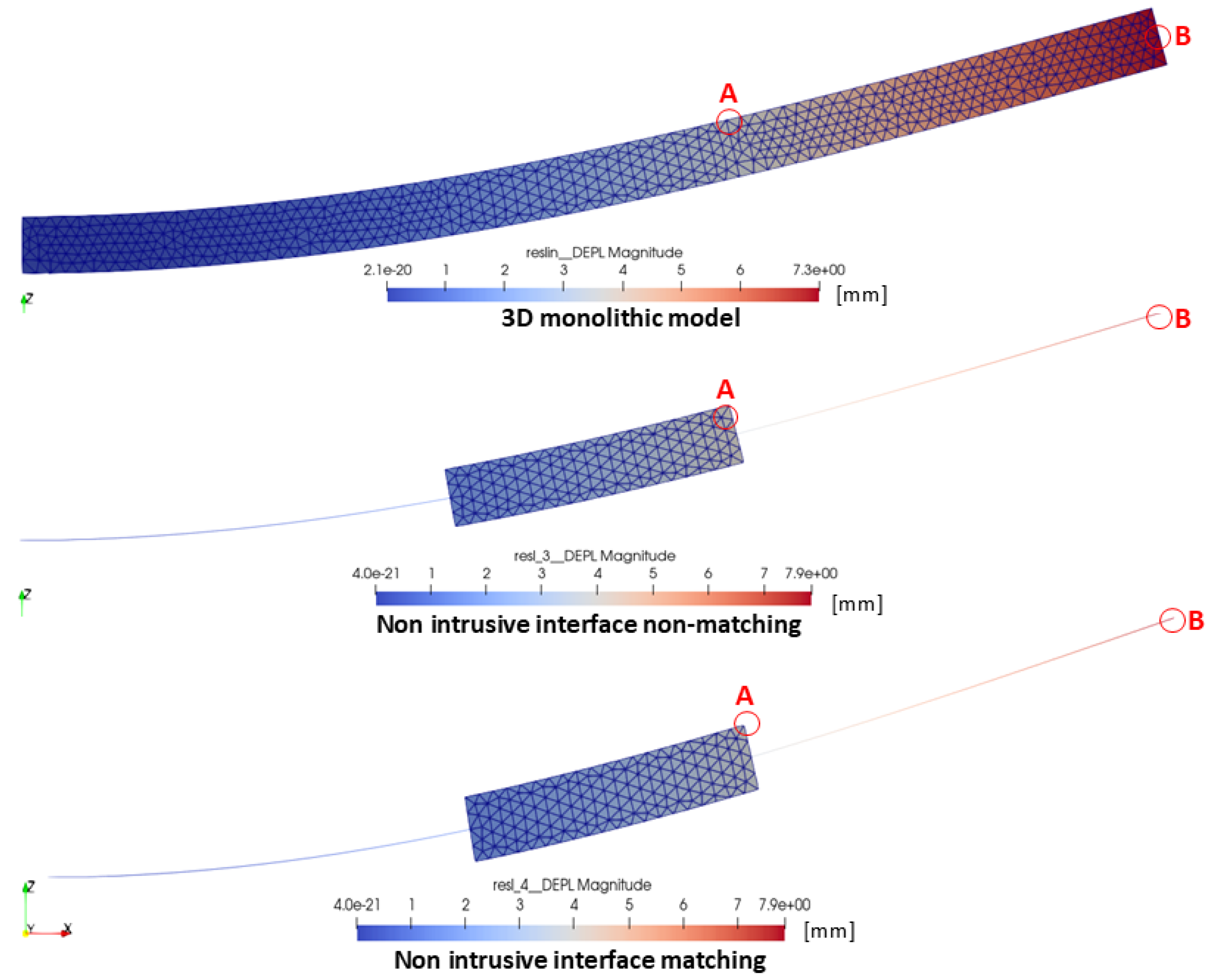
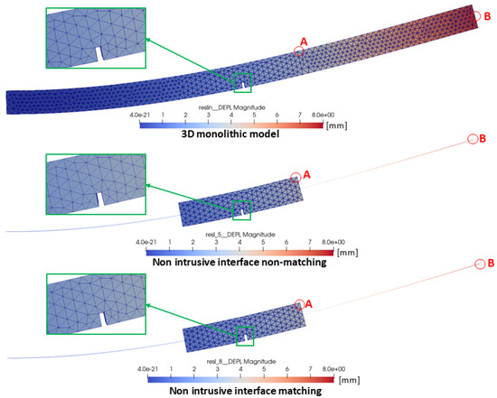
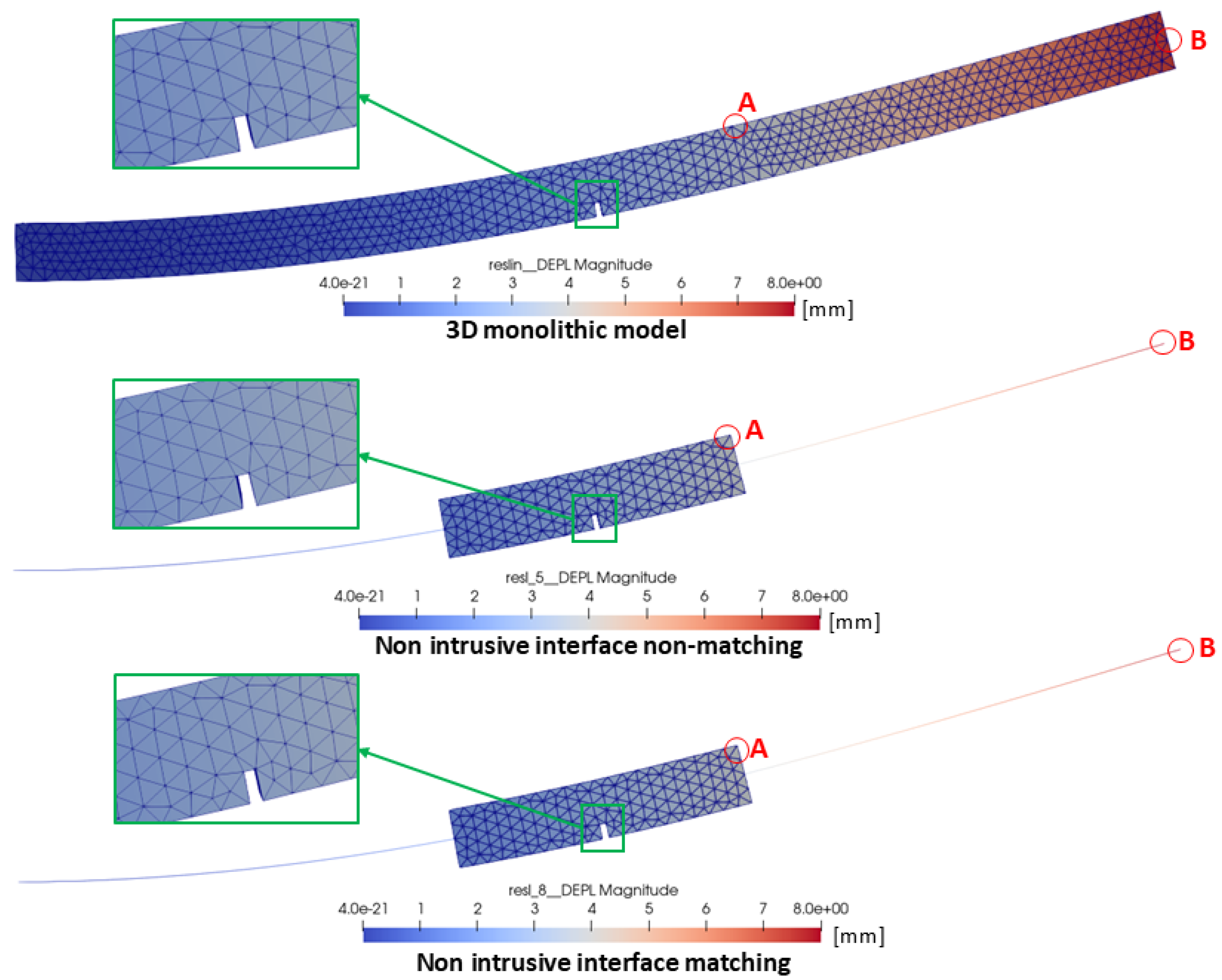
Figure 8 shows the deformation for the beam case under a linear state (without a crack) for the three simulations (top figure: monolithic beam, middle figure: non-intrusive non-matching interface, and bottom figure: non-intrusive matching interface), along with the displacements obtained at two points used for comparison to estimate the differences between the solutions.

Figure 8. Deformation of the cantilever beam: linear problem case.

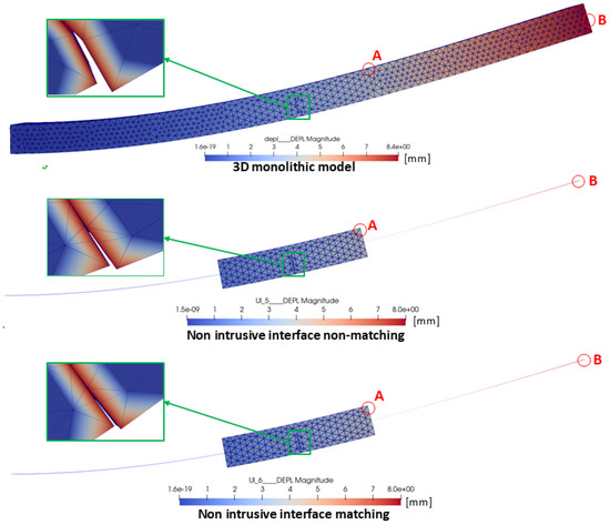
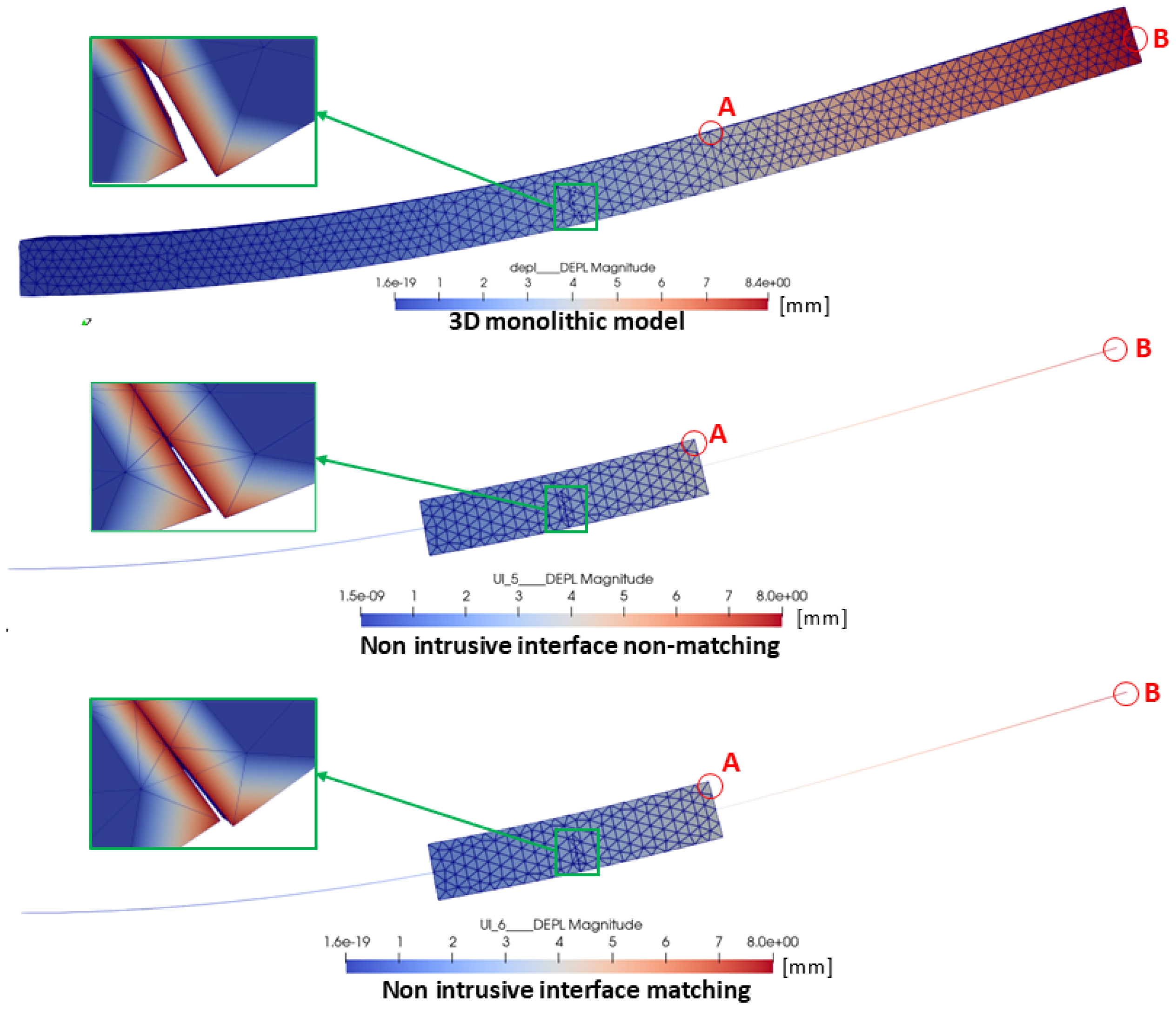
Figure 9 and Figure 10 present the deformation and the points where the displacements are compared for the cantilever beam case studies: linear with a notch and with crack propagation, respectively.

Figure 9. Deformation of the cantilever beam: linear problem with a notch.

Figure 10. Deformation of the cantilever beam: crack propagation problem.

Visual inspection of Figure 8, Figure 9 and Figure 10 confirms that the three methodologies produce qualitatively indistinguishable deformed shapes across the three variants: the maximum deflection at the free end is comparable, and no visible artifact appears at the boundary of the local domain in the non-matching case.

Two comparison points are used. Point A is located on the upper edge of the local model at the section where the local nonlinearity (notch or crack) is introduced ($x=2500$ mm, $y=-100$ mm, $z=200$ mm). Point B is located at the free end of the global beam ($x=4000$ mm, near the centroid of the section). These two points quantify the coupling accuracy locally (Point A, in the local model) and globally (Point B, in the global model).

To compare the displacements obtained from the different methodologies, the Euclidean norm was calculated, with the results presented in Table 1 and Table 2 for the displacements of the local and global models, respectively. The results show that the differences do not exceed 1 mm and are within the application of the Euler-Bernoulli deflection theory, which gives a deflection of 8 mm (Equation (22)).

$$\begin{array}{c}\hfill y={\displaystyle \frac{P{L}^3}{3EI}}\end{array}$$

(22)

Table 1. Norm of the displacements obtained using non-intrusive methodologies at the upper edge of the local model of the beam.

Methodology	Displacement Magnitude in the Local Beam Model
	Linear Beam	Beam with Notch	Cracked Beam
Monolithic 3D	3.403 mm	3.440 mm	3.894 mm
NI matching	3.684 mm	3.721 mm	3.713 mm
NI non-matching	3.669 mm	3.720 mm	3.710 mm

Table 2. Norm of the displacements obtained using non-intrusive methodologies at the free end of the beam.

Methodology	Displacement Magnitude at the Beam’s Free End
	Linear Beam	Beam with Notch	Cracked Beam
Monolithic 3D	7.33 mm	7.48 mm	8.38 mm
NI matching	7.86 mm	8.01 mm	7.98 mm
NI non-matching	7.85 mm	8.00 mm	7.97 mm

Meanwhile, Table 3 shows the percentage differences in the displacements at the upper edge of the local models compared to the norm of the displacement of the monolithic model (considered the most accurate solution) for the two non-intrusive methodologies and the three case studies. Table 4 does the same for the free end of the beam. The displacement error is calculated as shown in Equation (23).

$$\begin{array}{c}\hfill erro{r}_{desp}={\displaystyle \frac{\parallel u_m-u\parallel }{∥u_m∥}}\end{array}$$

(23)

where $∥u_m∥$ is the Euclidean norm of the displacement $(u_{mx},u_{my},u_{mz})$ of the monolithic model, and $\parallel u_m-u\parallel$ is the Euclidean norm of the difference between the displacements $(u_{mx},u_{my},u_{mz})$ and $(u_x,u_y,u_z)$ obtained from the corresponding local or global model.

Table 3. Normalized difference of the displacements obtained using non-intrusive methodologies at the upper edge of the local beam model.

Methodology	Displacement Difference in the Local Beam Model
	Linear Beam	Beam with Notch	Cracked Beam
% Diff. NI matching/mono.	8.255%	8.165%	4.649%
% Diff. NI non-matching/mono.	7.831%	8.132%	4.729%

Table 4. Normalized difference of the displacements obtained using non-intrusive methodologies at the free end of the beam.

Methodology	Displacement Difference at the Beam’s Free End
	Linear Beam	Beam with Notch	Cracked Beam
% Diff. NI matching/mono.	8.19%	8.07%	6.05%
% Diff. NI non-matching/mono.	8.08%	8.00%	6.08%

The relative errors reported in Table 3 and Table 4 stay below 10% in all variants. More importantly, the differences between the matching and the non-matching schemes themselves are below 0.5 percentage points (e.g., 8.255% vs. 7.831% on the upper edge of the local model in the linear case, 8.165% vs. 8.132% in the notched case), which shows that the introduction of the intermediate domain ${\mathsf{\Omega }}_I$ does not introduce a systematic error in the transferred kinematics. The proposed methodology therefore preserves the accuracy of the standard matching global/local analysis while removing the requirement that the local patch coincides with a node of the global mesh, restoring full freedom in the placement of the local domain.

Regarding the cracked beam, both non-intrusive schemes predict displacements very close to those of the notched beam. This is consistent with the geometry of the two configurations: the initial crack has the same depth as the notch (50 mm), and the crack fronts computed in the local model remained close to this initial depth, so the compliance introduced by the crack is similar to that of the notch. The larger increase observed in the monolithic model reflects that the crack evolution is computed in a different problem, the full 3D model instead of the local model driven by the coupling, in which the propagated crack geometry differs slightly, even though all analyses were performed with the same X-FEM settings (enrichment search, number of propagation steps and crack advance). In any case, the differences with respect to the monolithic solution remain below 10%, within the same range as for the linear and notched configurations. Since the X-FEM solver is used as a black box within the non-intrusive framework, this work focuses on validating the accuracy of the coupling methodology itself; a detailed assessment of the crack propagation predicted within the coupling is identified as a direction for future research.

3.2. Stress Comparison in the Notched Beam

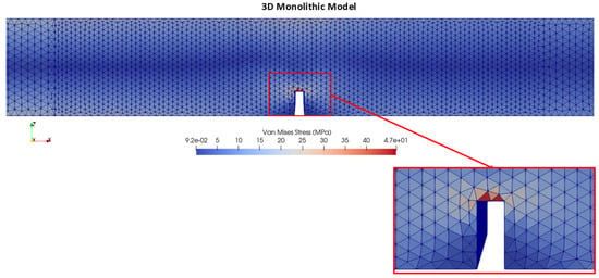
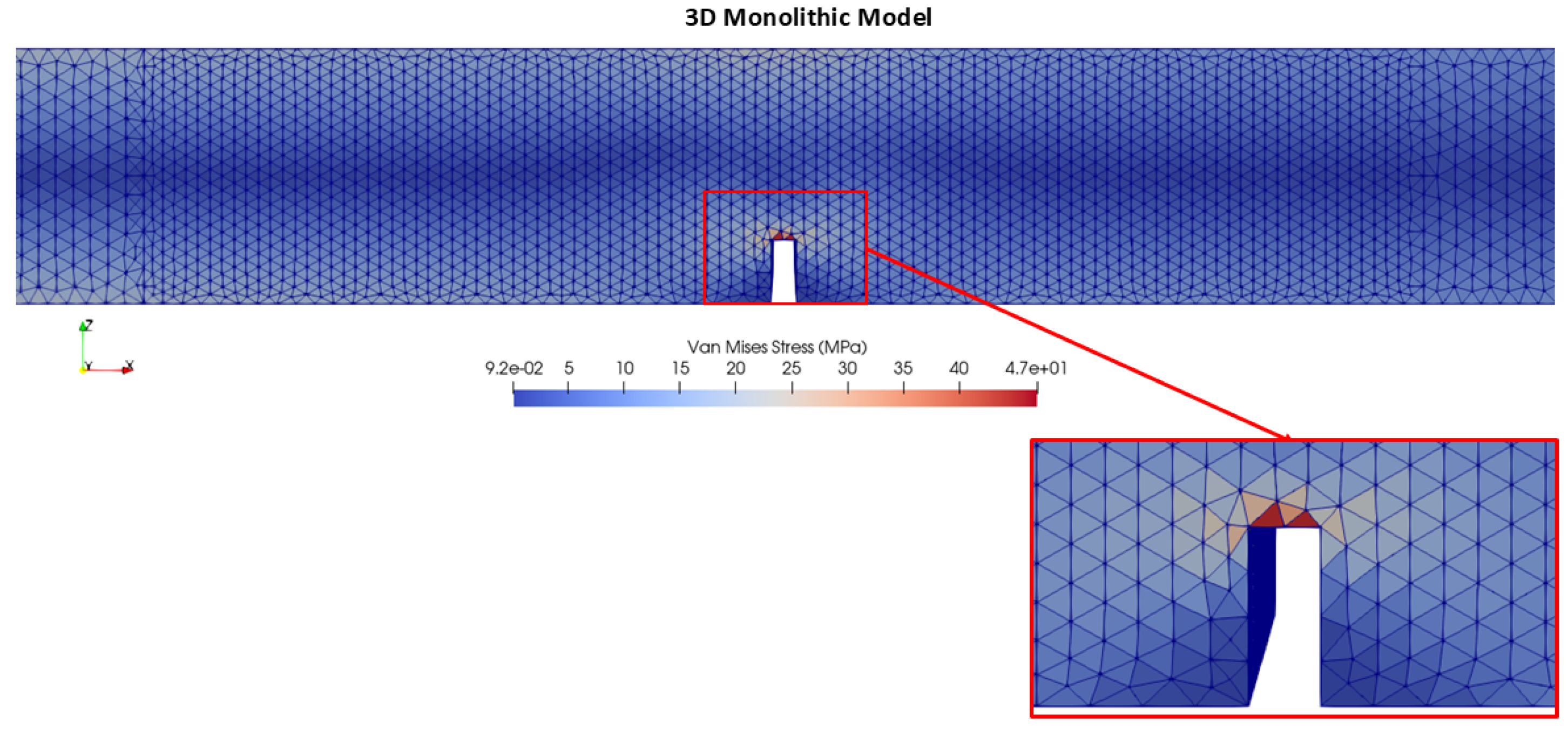
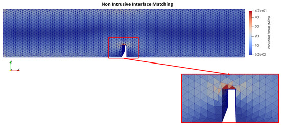
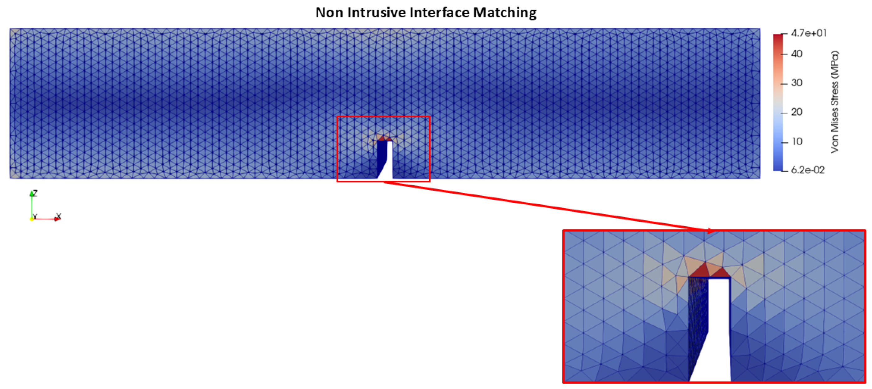
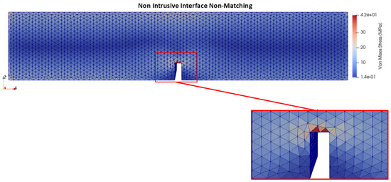
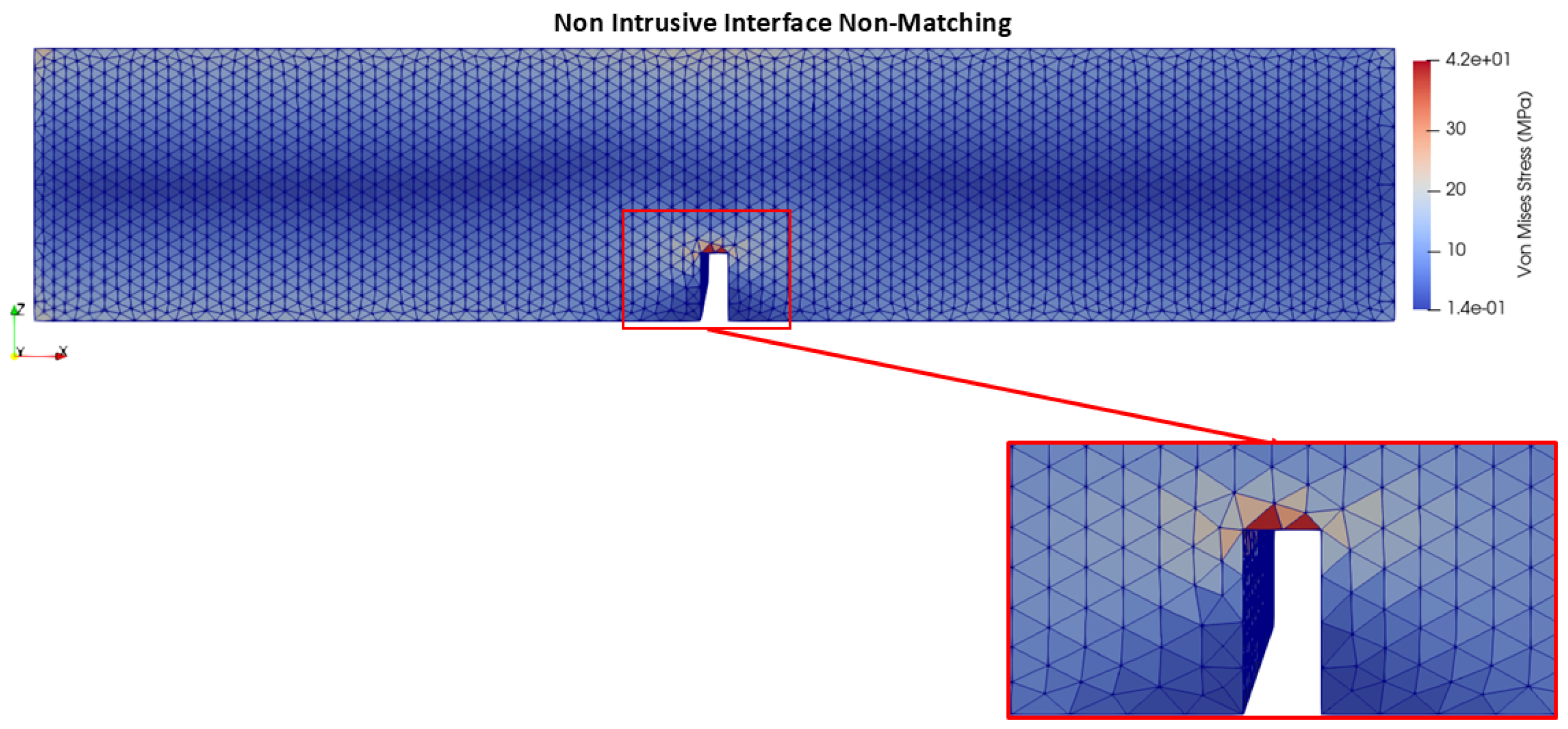
In order to observe the stress concentration effect in more detail, the local 3D model mesh was refined in the notch region, reaching a maximum edge length of 15 mm, with a total of 86,783 tetrahedral elements. This refinement was applied only to the local model ${\mathsf{\Omega }}_L$; the monolithic 3D model retains a coarser element size away from the notch, with local refinement limited to the same region for a consistent comparison. The resulting Von Mises stress distribution can be observed in Figure 11, Figure 12, and Figure 13 for the monolithic model, the global/local non-intrusive matching interface, and the global/local non-intrusive non-matching interface, respectively. In all cases, the maximum stress concentration occurs at the base of the notch, as expected due to the geometric discontinuity.

Figure 11. Von Mises stress distribution around the notch region for the 3D monolithic model.

Figure 12. Von Mises stress distribution around the notch region using the global/local non-intrusive matching interface.

Figure 13. Von Mises stress distribution around the notch region using the global/local non-intrusive non-matching interface.

Table 5 shows the maximum Von Mises stress obtained for each methodology, along with the percentage error with respect to the monolithic model.

Table 5. Maximum Von Mises stress obtained using non-intrusive methodologies for the notch problem.

Methodology	Maximum Von Mises Stress (MPa)	% Diff. w.r.t. Monolithic
3D Monolithic	46.8826	—
NI Matching	46.8712	0.02%
NI Non-matching	41.5297	11.42%

As shown in Table 5, the matching interface approach yields a maximum stress value very close to the monolithic model, with a difference of only 0.02%. The non-matching interface approach, on the other hand, results in a lower maximum stress value, with a difference of approximately 11.42% with respect to the monolithic model.

This difference is related to the way the inner interface $\gamma$ is handled in the proposed algorithm. At each iteration, the displacements imposed on the local model at $\gamma$ are obtained from the intermediate model solved only with the displacements of $\Gamma$ and the external loads (step 4), that is, from an elastic, undamaged beam segment. The correction forces $P_I$, which represent the non-linear behaviour of the local model, are applied to the intermediate model afterwards (step 10), where they update the reactions transferred to the global model at $\Gamma$; the displacements imposed at $\gamma$ are therefore determined before this correction is applied. Consequently, the convergence criterion ($\eta <{10}^{-6}$) enforces the balance at $\Gamma$, while the kinematics imposed at $\gamma$ correspond to those of the undamaged beam segment. Since the local model and its position are identical in both schemes, and the matching scheme reproduces the monolithic peak stress within 0.02%, the displacements of the matching global model at the same sections can be used as a reference. At the last iteration, the relative rotation between the two sections of $\gamma$ imposed on the local model in the non-matching scheme is 6.9% lower than in the matching scheme, whereas the intermediate model after applying $P_I$ differs by only 1.1%. The local model is therefore subjected to less bending across the notch than required, which reduces the peak stress, while integral quantities such as displacements, governed by the corrected global model, remain accurate. For the same reason, the discrepancy originates in the kinematics transferred through $\gamma$ rather than in the spatial discretisation of the local model, so refining its mesh would not be expected to reduce it.

Despite this difference, the overall stress distribution pattern remains consistent across all three approaches, and the location of the maximum stress concentration is correctly captured in every case.

3.3. Validation of the Methodology Using the Framed-Structure Results

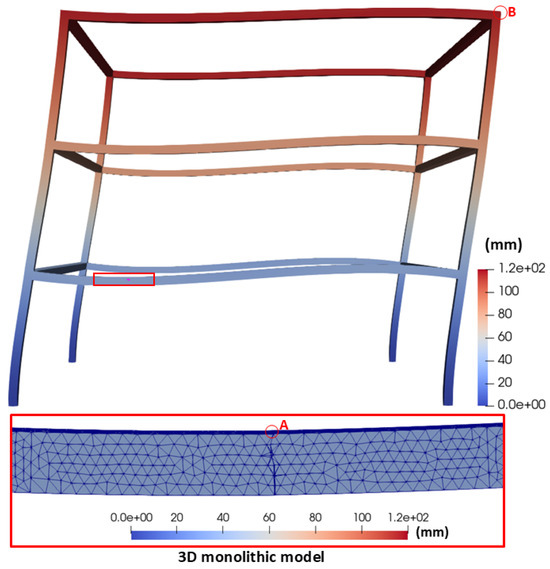
As in Section 3.1, the validation of the methodology for the case study of the frame structure is carried out by comparing the displacements obtained from the different methodologies at two points: near the crack and at the top of the frame. In this case, only the structure with crack growth is considered.

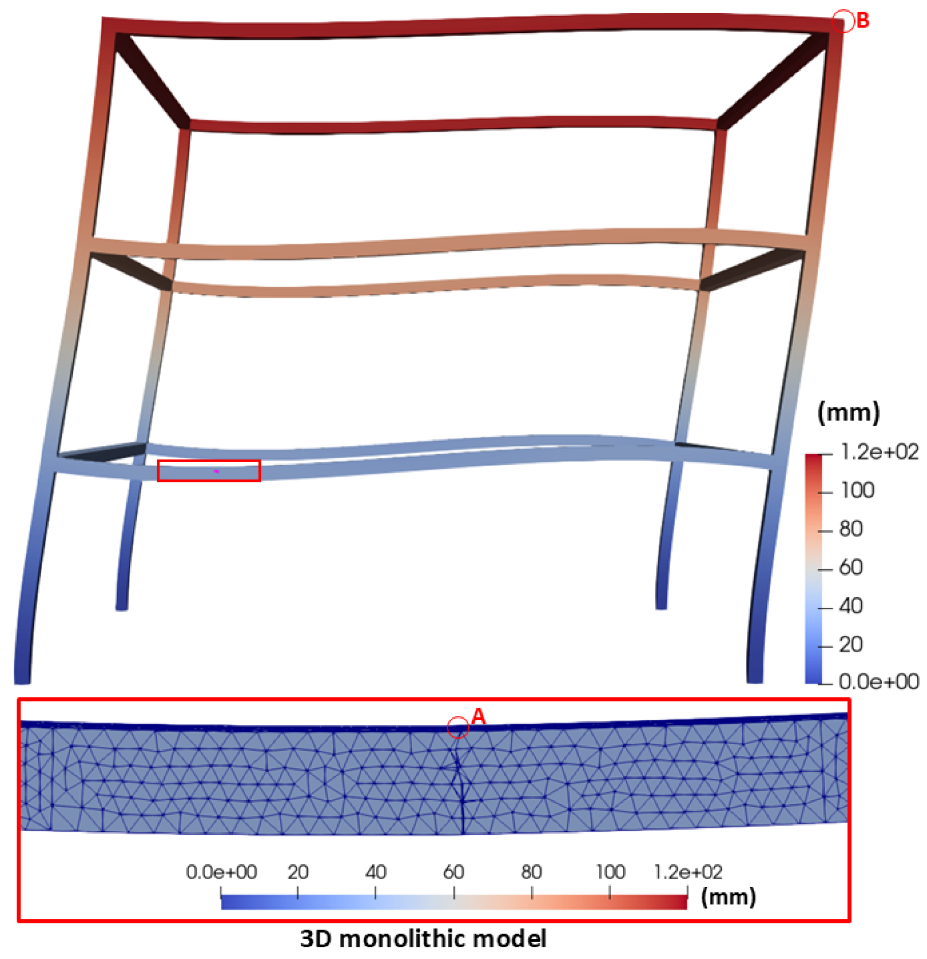
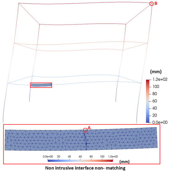
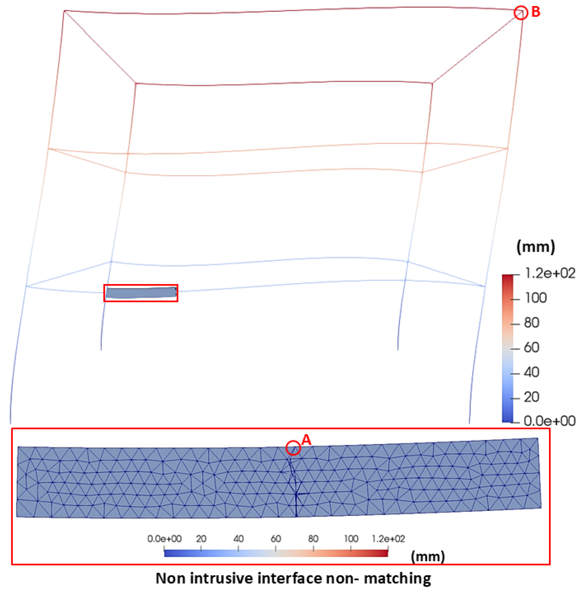
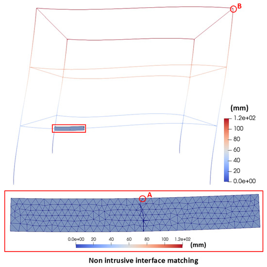
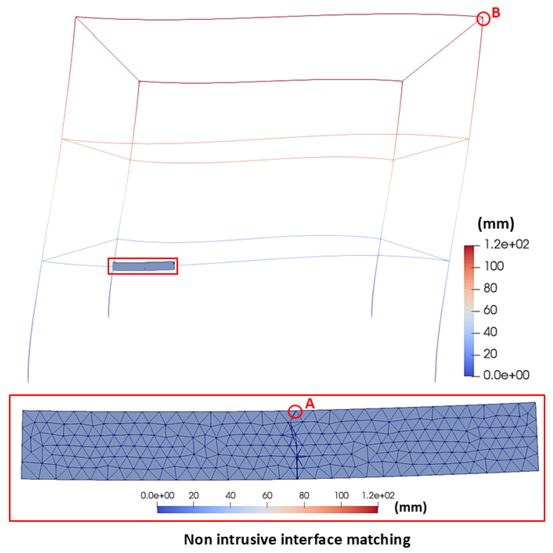
The deformed shape of the problem with crack growth can be seen in Figure 14, Figure 15, and Figure 16 for the monolithic model, global/local non-matching interface, and global/local matching interface, respectively. These figures also show the crack obtained in each simulation and the displacement at the comparison point.

Figure 14. Deformed shape of the monolithic frame model for the crack growth problem.

Figure 15. Deformed shape of the frame with a non-matching interface for the crack growth problem.

Figure 16. Deformed shape of the frame with a matching interface for the crack growth problem.

Table 6 shows the results of calculating the Euclidean norm of the displacements near the crack for the frame with crack growth. Similar to the clamped beam case, the results show a small variation among the different methodologies, with the absolute difference with respect to the monolithic model not exceeding 1 mm. To complement this local error assessment, the displacement was also compared at the top of the frame, the point farthest from the supports, following the same criterion used for the free end of the beam. Table 7 shows the corresponding results.

Table 6. Norm of displacements and normalized difference obtained using non-intrusive methodologies near the crack of the cracked frame model.

Methodology	Displacement Magnitude	% Diff. w.r.t. Monolithic
3D Monolithic	37.586 mm	—
NI matching	36.630 mm	2.967%
NI non-matching	38.304 mm	2.944%

Table 7. Norm of displacements and normalized difference obtained using non-intrusive methodologies at the top of the frame of the cracked frame model.

Methodology	Displacement Magnitude	% Diff. w.r.t. Monolithic
3D Monolithic	116.35 mm	—
NI matching	116.82 mm	0.76%
NI non-matching	119.48 mm	2.77%

The errors obtained in the crack growth case remain below 3% at both comparison points, for both non-intrusive schemes (2.967% and 2.944% near the crack, for matching and non-matching respectively; 0.76% and 2.77% at the top of the frame), confirming the consistency of the proposed methodology with the reference monolithic solution even in the presence of localized nonlinear damage. The two schemes perform similarly near the crack, whereas the matching scheme is more accurate than the non-matching scheme at the top of the frame. Overall, the non-matching scheme reproduces the reference solution within the same order of accuracy as the matching scheme, while offering the added flexibility of a coupling interface that does not need to coincide with a node of the global mesh, which is particularly relevant for practical applications where generating matching meshes between global and local models is not always feasible.

To further assess the predictive capability of the non-intrusive schemes for the global structural response, the force-displacement response at the top of the frame was obtained for the three models, keeping the crack geometry fixed at the converged configuration (initial crack length of 50 mm, three propagation steps). Table 8 shows this response for applied loads between 25 and 100 kN. As expected for a linear elastic fracture mechanics problem with a fixed crack geometry and predetermined 3 propagation steps, the response of each model exhibits nearly a linearized behavior over the entire load range, and the three schemes remain close to each other, confirming that the proposed methodology captures the global structural response of the cracked frame with good accuracy.

Table 8. Force-displacement response at the top of the cracked frame (crack length 50 mm, three propagation steps), for the three models.

Applied Load (kN)	3D Monolithic (mm)	NI Matching (mm)	NI Non-Matching (mm)
25	29.087	29.206	29.871
50	58.175	58.412	59.741
75	87.262	87.617	89.612
100	116.350	116.823	119.482

The loss of stiffness caused by the crack was compared for the three models at the top of the frame, the same point used above. The stiffness was computed as the secant stiffness $K=P/\delta$, using the converged displacement $\delta$ at the applied load $P=100$ kN, with and without the crack. Table 9 reports these values and the resulting stiffness loss. The matching scheme predicts a stiffness loss close to that of the monolithic reference (0.23% versus 0.31%), whereas the non-matching scheme overestimates it by nearly an order of magnitude (2.45%). This is consistent with the mechanism discussed in Section 3.2 and Section 3.4: since the kinematics imposed on the local model at $\gamma$ are not corrected for the non-linear behaviour of the crack, the non-matching scheme is more sensitive than the matching scheme to the presence of the crack, even though the two schemes are equally accurate in the absence of damage.

Table 9. Stiffness loss at the top of the frame caused by the crack (length 50 mm, three propagation steps), for an applied load of 100 kN.

Model	Linear Stiffness (kN/mm)	Stiffness Loss
3D Monolithic	0.8621	0.31%
NI matching	0.8579	0.23%
NI non-matching	0.8580	2.45%

3.4. Convergence Analysis

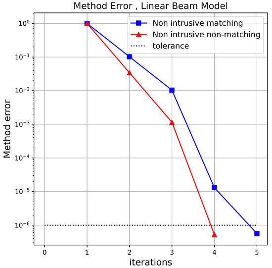
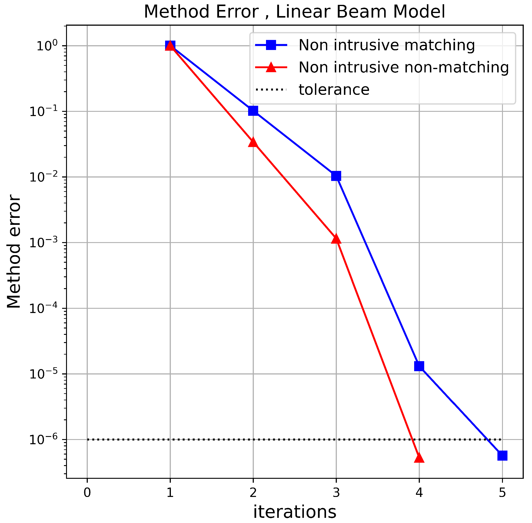
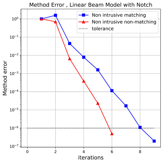
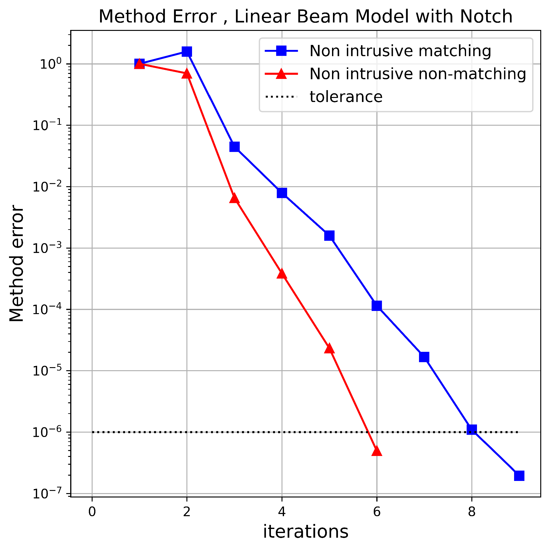
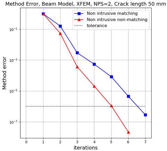
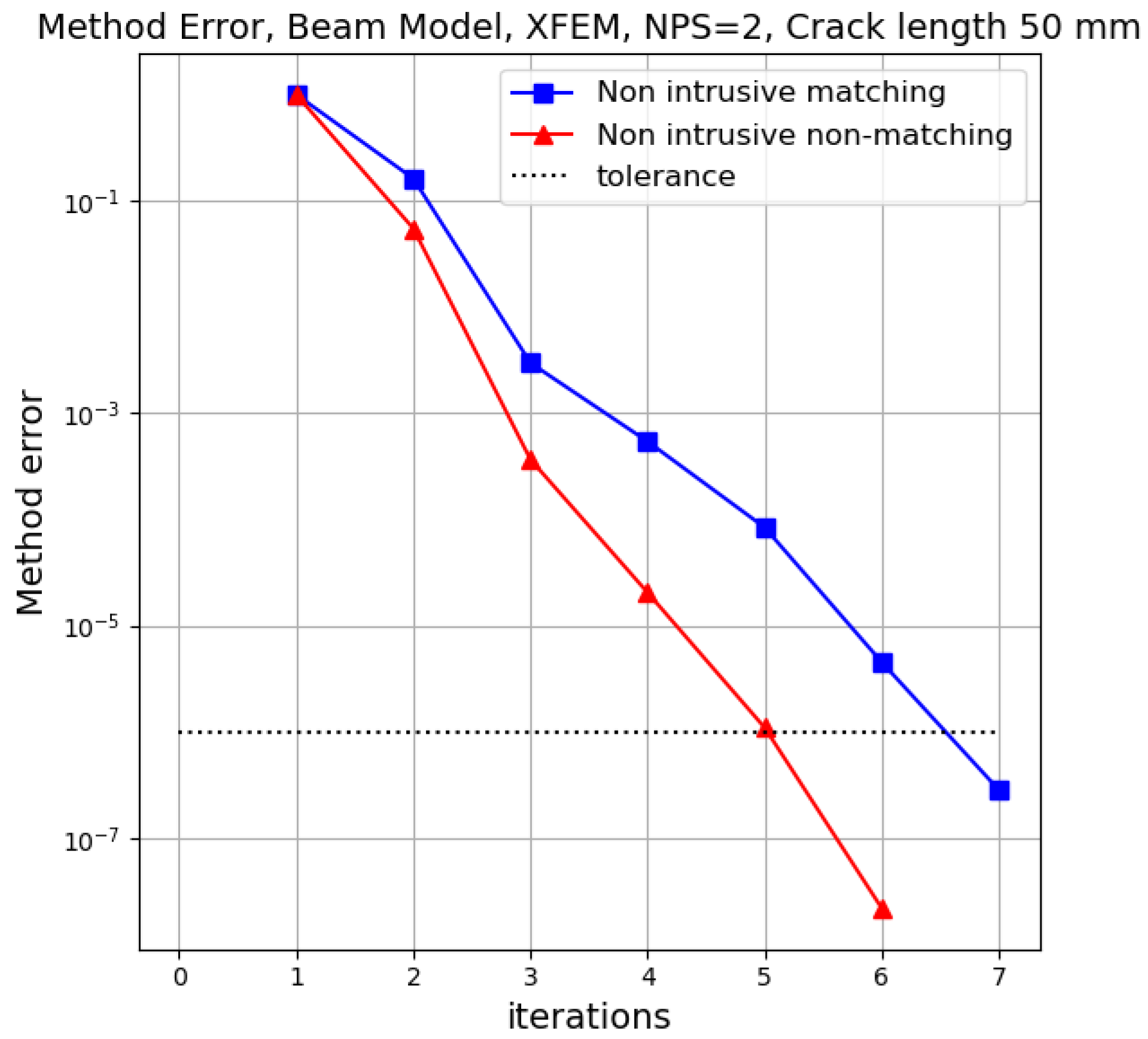
In Figure 17, Figure 18 and Figure 19, the number of iterations required for the global/local analysis to converge as a function of the methodology error ($\eta$) is shown.

Figure 17. Comparison of convergence in the linear beam problem.

Figure 18. Comparison of convergence in the notched beam problem.

Figure 19. Comparison of convergence in the cracked beam problem.

It can be observed that the global/local analysis with a non-matching interface converges in fewer iterations than the matching interface for all cases, with up to three fewer iterations in the notched beam case.

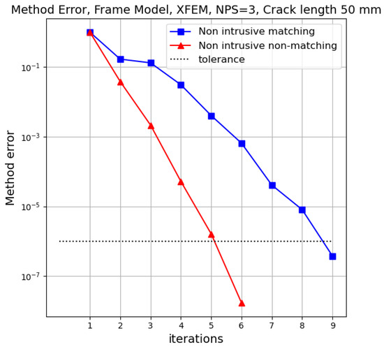
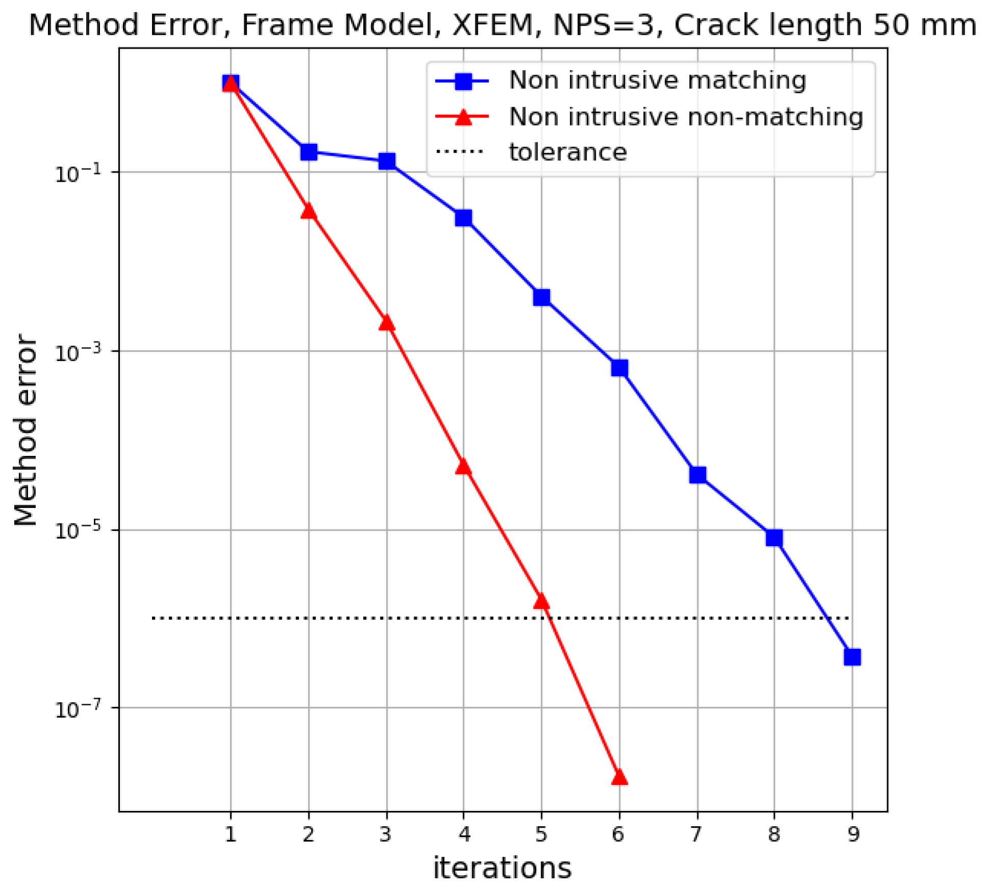
On the other hand, Figure 20 shows the iterations and methodology error for the frame structure with crack growth. In this case, the non-matching interface also converges in fewer iterations than the matching interface reducing the required iterations by 33%.

Figure 20. Comparison of convergence in the cracked frame problem.

This reduction is consistent across all cases. In non-intrusive global/local coupling, the convergence rate depends on the contrast between the local and the global stiffness [24,25]. In the matching scheme, the segment replaced at $\Gamma$ coincides with the local model, so the stiffness reduction caused by the notch or crack affects the whole replaced segment. In the non-matching scheme, the segment replaced at $\Gamma$ also includes the undamaged parts of the intermediate model between $\Gamma$ and $\gamma$, so the relative stiffness reduction seen by the global model is smaller than in the matching scheme, which is consistent with the smaller number of iterations. However, the faster convergence may also be partly related to how the algorithm enforces the balance only at $\Gamma$, while the kinematics at $\gamma$ follow directly from the intermediate model, as discussed in Section 3.2. The reduction in iterations should therefore be interpreted together with the local stress accuracy discussed there, since it comes together with the reduced accuracy of the local stress field.

The reduction in the number of iterations required for the global/local analysis to converge can be expressed in terms of computational time. Table 10 presents the time required to solve the crack propagation problem in the frame model.

Table 10. Computational time differences in global/local analysis with matching and non-matching interfaces.

Methodology	Computation Time (s)	Time Saved vs. Monolithic (%)
3D Monolithic	673.51 s	—
NI Matching	310.81 s	53.86%
NI Non-Matching	214.24 s	68.19%

As shown, using a non-matching global/local analysis reduces the computational time required to solve the problem by 68.19% compared to the monolithic model. The matching global/local analysis also reduces the computational time, albeit to a lesser extent, achieving a 53.86% reduction relative to the monolithic model. Notably, as the structure size increases, the matching interface analysis tends to achieve better performance, as seen in [36]. This indicates that using the methodology proposed in this work could further reduce analysis time, as it offers better performance without compromising the accuracy of the displacement field.

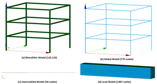
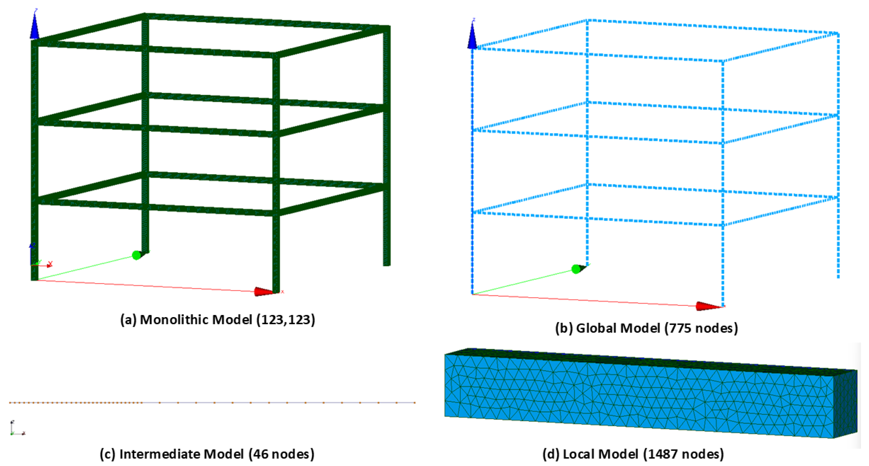
The reduction in computational time observed in the global/local approach can also be explained by the significant reduction in the number of degrees of freedom (DOF) involved in the analysis. Figure 21 shows the discretization of the four models involved in the frame structure analysis, illustrating the difference in mesh density and element type between the monolithic model and the global, intermediate, and local models used in the global/local coupling approach. Table 11 presents the total DOF for the monolithic model and for the two global/local coupling strategies.

Figure 21. Discretization of the frame structure: (a) monolithic model (123,123 nodes); (b) global model (775 nodes); (c) intermediate model (46 nodes); (d) local model (1487 nodes).

Table 11. Number of degrees of freedom (DOF) of the monolithic and global/local models for the frame structure.

Methodology	Total DOF	% Reduction w.r.t. Monolithic
3D Monolithic	369,369	—
NI Matching (Global + Local)	9111	97.53%
NI Non-matching (Global + Intermediate + Local)	9387	97.46%

While the 3D monolithic model has a total of 369,369 DOF, the matching interface approach, composed of the global and local models, requires solving a problem with only 9111 DOF, representing a reduction of approximately 97.53%. The non-matching interface approach, which additionally includes the intermediate model, results in a total of 9387 DOF, corresponding to a reduction of approximately 97.46%. The non-matching approach involves 276 additional DOF due to the intermediate model (46 nodes after meshing its three segments), i.e., a 3.03% increase with respect to the matching approach. This increment adds only a small overhead to the cost of each coupling iteration: the average time per iteration is 34.53 s for the matching approach and 35.71 s for the non-matching approach, a difference of 3.4%. At the same time, the number of iterations decreases from 9 to 6, so the total computation time is reduced by 31% (Table 10). In other words, the intermediate model adds a small, fixed cost to each iteration, while each iteration saved directly reduces the number of nonlinear solves of the local model, which is the most expensive step of the analysis. Overall, these results confirm that the much smaller problem solved at each iteration, compared with the monolithic model, is a key factor contributing to the lower computational cost of the global/local methodology.

4. Discussion

This work presented a three-level non-intrusive global–local coupling strategy, adding an intermediate 1D beam model between the global and local domains so that the local patch can be placed independently of the global mesh nodes. Two case studies were used for validation: a cantilever beam and a three-story framed structure, both analyzed under linear, notched, and crack-propagation conditions and compared against a 3D monolithic reference and the matching-interface approach from [36].

Displacement errors for the non-matching scheme stayed below 10% relative to the monolithic solution in every case, in line with what was previously reported for the matching interface [36]. The intermediate domain therefore does not compromise the accuracy of the transferred displacements, and removes the need for the local patch to coincide with an existing global node.

The stresses in the notched beam behaved differently. While the matching scheme reproduced the monolithic peak Von Mises stress within 0.02%, the non-matching scheme underestimated it by 11.42%. As discussed in Section 3.2, this is because the displacements imposed on the local model at $\gamma$ are obtained from the intermediate model solved with the displacements of $\Gamma$ only, that is, from the undamaged beam; the correction forces $P_I$ are applied afterwards to update the reactions transferred to $\Gamma$, which is the balance enforced by the convergence criterion. As a result, the relative rotation imposed across the notch is 6.9% lower than in the matching scheme. The effect is confined to the local stress field, while the displacement field and the location of the maximum stress remain accurate. Carrying $P_I$ over to the intermediate solve that provides the displacements at $\gamma$, or introducing a Robin-type condition on $\gamma$ [24], are natural ways to enforce the balance at both interfaces and will be addressed in future work. A detailed comparison of the convergence conditions of both schemes, including the effect of the convergence tolerance, is also left for future work.

The efficiency gains were clearer. For the frame model, the non-matching approach cut the computation time by 68.19% relative to the monolithic model, versus 53.86% for the matching interface. This is consistent with the drop in degrees of freedom: the monolithic model needed 369,369 DOF, while the non-matching system (global + intermediate + local) needed only 9387, a 97.46% reduction, close to the 97.53% obtained with matching. The intermediate model adds a small number of extra DOF compared to the matching scheme, but this is negligible next to the overall reduction and does not cancel out the gain from fewer iterations.

The faster convergence of the non-matching scheme can be related to the stiffness contrast at $\Gamma$, which governs the convergence rate of non-intrusive coupling [24,25]. Since the segment replaced at $\Gamma$ includes the undamaged parts of the intermediate model, the relative stiffness reduction seen by the global model is smaller than in the matching scheme. This benefit, however, may partly result from how the balance at $\gamma$ is enforced, which is also the origin of the lower peak stress obtained in Section 3.2. Enforcing the balance at both interfaces, as proposed above, would also allow the convergence gain to be assessed at equal local accuracy.

Compared to the matching-interface version in [36], this method adds one practical advantage: the local patch can be sized and placed without depending on the existing global discretization. This matters for real structures, such as an existing building modeled in commercial software, where remeshing the global model is often not an option. The added cost, one extra 1D domain per coupling region, is negligible in terms of both DOF and computational overhead, as shown in the frame case.

Future work could go in several directions: testing the method under sequential or cyclic loading to check how the force compensation scheme handles load reversal; applying the discriminant criterion from [25] to size the local and intermediate models within the three-level scheme; enforcing the balance at the inner interface $\gamma$, as discussed above; and implementing the method in commercial software, as done for the matching interface in [36], to test it in industrial settings and with other nonlinear behaviors such as plasticity.

5. Conclusions

This work presented and validated a three-level non-intrusive global-local coupling strategy with non-matching interfaces for crack propagation in beam-solid structures. Its main contribution is an intermediate 1D beam domain that restores full freedom in the placement of the local 3D patch, without requiring the local mesh to coincide with a node of the global model and without modifying the global model itself.

For the three-story framed structure, both non-intrusive schemes reduce the total number of degrees of freedom by more than 97% with respect to the 3D monolithic reference (97.53% for the matching scheme and 97.46% for the non-matching scheme), and the computation time by 53.86% and 68.19%, respectively, while keeping displacement errors below 3% at both the section near the crack and the top of the frame. The non-matching scheme converges in fewer iterations than the matching scheme (a 33% reduction), which is related to the lower stiffness contrast seen by the global model when part of the compensation forces are transferred through the undamaged segments of the intermediate domain.

This benefit comes together with a limitation: the algorithm enforces the equilibrium condition at the outer interface $\Gamma$, while the kinematics transferred to the local model at the inner interface $\gamma$ follow directly from the undamaged intermediate beam. This was found to underestimate the peak stress at the notch by 11.42% in the non-matching scheme, while the displacement field remained accurate. The formulation also relies on a rigid-section kinematic assumption at the beam-to-solid interfaces, and the validation was limited to two case studies with a single initial crack, under monotonic loading, within a linear elastic fracture mechanics framework.

Enforcing the equilibrium condition at both $\Gamma$ and $\gamma$ is identified as the main direction for future work to improve local stress accuracy, for instance by carrying the correction forces over to the intermediate solve, through a Robin-type coupling condition, or through a joint convergence criterion evaluated at both interfaces. A detailed comparison of the convergence conditions of the matching and non-matching schemes is also left for future work, in particular whether increasing the number of local-loop iterations or tightening the convergence tolerance reduces the discrepancy identified above. Extending the implementation to commercial software, such as SAP2000, would support its applicability to large structures with localized non-linearities using tools already available in industry; extending the approach to phase-field crack propagation models is another promising direction, given the potential of the proposed coupling to reduce the computational cost of such methods in large structures.

References

- Nonlinear Continuum Mechanics and Phenomenological Plasticity Models; Springer New York: New York, NY, 1998; pp. 240–275. [CrossRef] [Scilit]
- Wriggers, P.; Zavarise, G. Computational Contact Mechanics. In Encyclopedia of Computational Mechanics; Wiley: Hoboken, NJ, USA, 2004; Chapter 6; pp. 195–226. [Google Scholar] [CrossRef] [Scilit]
- Crisfield, M. Non-Linear Finite Element Analysis of Solids and Structures, Essentials; Non-Linear Finite Element Analysis of Solids and Structures; Wiley: Hoboken, NJ, USA, 1991. [Google Scholar]
- Bathe, K.J. Finite Element Procedures in Engineering Analysis; Prentice Hall: Upper Saddle River, NJ, USA, 2006. [Google Scholar]
- Belytschko, T.; Liu, W.; Moran, B.; Elkhodary, K. Nonlinear Finite Elements for Continua and Structures; Wiley: Hoboken, NJ, USA, 2014. [Google Scholar]
- Farhat, C.; Roux, F.X. A method of finite element tearing and interconnecting and its parallel solution algorithm. Int. J. Numer. Methods Eng. 1991, 32, 1205–1227. [Google Scholar] [CrossRef] [Scilit]
- Mandel, J. Balancing domain decomposition. Commun. Numer. Methods Eng. 1993, 9, 233–241. [Google Scholar] [CrossRef] [Scilit]
- Toselli, A.; Widlund, O. Domain Decomposition Methods-Algorithms and Theory; Springer Series in Computational Mathematics; Springer: Berlin/Heidelberg, Germany, 2005; Volume 34. [Google Scholar]
- Pebrel, J.; Rey, C.; Gosselet, P. A nonlinear dual domain decomposition method: Application to structural problems with damage. Int. J. Multiscale Comput. Eng. 2008, 6, 251–262. [Google Scholar] [CrossRef] [Scilit]
- Gosselet, P.; Rey, C. Non-overlapping domain decomposition methods in structural mechanics. Arch. Comput. Methods Eng. 2006, 13, 515–572. [Google Scholar] [CrossRef] [Scilit]
- Whitcomb, J.D. Iterative global/local finite element analysis. Comput. Struct. 1991, 40, 1027–1031. [Google Scholar] [CrossRef] [Scilit]
- Liu, Z.; Correia, J.A.F.O.; Carvalho, H.; Mourão, A.; de Jesus, A.M.P.; Calçada, R.; Berto, F. Global-local fatigue assessment of an ancient riveted metallic bridge based on submodelling of the critical detail. Fatigue Fract. Eng. Mater. Struct. 2019, 42, 546–560. [Google Scholar] [CrossRef] [Scilit]
- Gendre, L.; Allix, O.; Gosselet, P.; Comte, F. Non-intrusive and exact global/local techniques for structural problems with local plasticity. Comput. Mech. 2009, 44, 233–245. [Google Scholar] [CrossRef] [Scilit]
- Duval, M.; Passieux, J.c.; Salaün, M.; Guinard, S. Non-intrusive Coupling: Recent Advances and Scalable Nonlinear Domain Decomposition. Arch. Comput. Methods Eng. 2016, 23, 17–38. [Google Scholar] [CrossRef] [Scilit]
- Gosselet, P.; Blanchard, M.; Allix, O.; Guguin, G. Non-invasive global-local coupling as a Schwarz domain decomposition method: Acceleration and generalization. Adv. Model. Simul. Eng. Sci. 2018, 5, 4. [Google Scholar] [CrossRef] [Scilit]
- Allix, O.; Gosselet, P. Non Intrusive Global/Local Coupling Techniques in Solid Mechanics: An Introduction to Different Coupling Strategies and Acceleration Techniques. In Modeling in Engineering Using Innovative Numerical Methods for Solids and Fluids; De Lorenzis, L., Düster, A., Eds.; CISM International Centre for Mechanical Sciences Courses and Lectures; Springer Nature Switzerland AG: Cham, Switzerland, 2020; Volume 599, pp. 203–220. [Google Scholar] [CrossRef] [Scilit]
- Bouclier, R.; Passieux, J.C.; Salaün, M. Local enrichment of NURBS patches using a non-intrusive coupling strategy: Geometric details, local refinement, inclusion, fracture. Comput. Methods Appl. Mech. Eng. 2016, 300, 1–26. [Google Scholar] [CrossRef] [Scilit]
- Passieux, J.C.; Ladevèze, P.; Néron, D. A scalable time-space multiscale domain decomposition method: Adaptive time scales separation. Comput. Mech. 2010, 46, 621–633. [Google Scholar] [CrossRef] [Scilit]
- Liu, Y.J.; Sun, Q.; Fan, X.L. A non-intrusive global/local algorithm with non-matching interface: Derivation and numerical validation. Comput. Methods Appl. Mech. Eng. 2014, 277, 81–103. [Google Scholar] [CrossRef] [Scilit]
- Moës, N.; Dolbow, J.; Belytschko, T. A finite element method for crack growth without remeshing. Int. J. Numer. Methods Eng. 1999, 46, 131–150. [Google Scholar] [CrossRef] [Scilit]
- Guidault, P.; Allix, O.; Champaney, L.; Cornuault, C. A multiscale extended finite element method for crack propagation. Comput. Methods Appl. Mech. Eng. 2008, 197, 381–399. [Google Scholar] [CrossRef] [Scilit]
- Bourdin, B.; Francfort, G.A.; Marigo, J.J. The variational approach to fracture. J. Elast. 2008, 91, 5–148. [Google Scholar] [CrossRef] [Scilit]
- Birner, M.; Diehl, P.; Lipton, R.; Schweitzer, M.A. A multiscale fracture model using peridynamic enrichment of finite elements within an adaptive partition of unity: Experimental validation. Mech. Res. Commun. 2024, 137, 104275. [Google Scholar] [CrossRef] [Scilit]
- Gendre, L.; Allix, O.; Gosselet, P. A two-scale approximation of the Schur complement and its use for non-intrusive coupling. Int. J. Numer. Methods Eng. 2011, 87, 889–905. [Google Scholar] [CrossRef] [Scilit]
- Jaque-Zurita, M.; Hinojosa, J.; Castillo-Ibarra, E.; Fuenzalida-Henríquez, I. Discriminant Analysis Based on the Patch Length and Crack Depth to Determine the Convergence of Global–Local Non-Intrusive Analysis with 1D-to-3D Coupling. Symmetry 2023, 15, 2068. [Google Scholar] [CrossRef] [Scilit]
- Aitken, A.C. On Bernoulli’s numerical solution of algebraic equations. Proc. R. Soc. Edinb. 1926, 46, 289–305. [Google Scholar] [CrossRef] [Scilit]
- Irons, B.M.; Tuck, R.C. A version of the Aitken accelerator for computer iteration. Int. J. Numer. Methods Eng. 1969, 1, 275–277. [Google Scholar] [CrossRef] [Scilit]
- Fillmore, T.B.; Wu, Z.; Vega, M.A.; Hu, Z.; Todd, M.D. A surrogate model to accelerate non-intrusive global–local simulations of cracked steel structures. Struct. Multidiscip. Optim. 2022, 65, 208. [Google Scholar] [CrossRef] [Scilit]
- Bueno, A.; Silveira Filho, N.; Barros, F. A non-intrusive multiscale framework for 2D analysis of local features by GFEM—A thorough parameter investigation. Finite Elem. Anal. Des. 2024, 242, 104258. [Google Scholar] [CrossRef] [Scilit]
- Steinbrecher, I.; Mayr, M.; Grill, M.J.; Kremheller, J.; Meier, C.; Popp, A. A mortar-type finite element approach for embedding 1D beams into 3D solid volumes. Comput. Mech. 2020, 66, 1377–1398. [Google Scholar] [CrossRef] [Scilit]
- Li, H.; Avecillas-Leon, J.; Shauer, N.; Duarte, C. A non-intrusive iterative generalized finite element method for multiscale coupling of 3-D solid and shell models. Comput. Methods Appl. Mech. Eng. 2022, 402, 115408. [Google Scholar] [CrossRef] [Scilit]
- Bai, X.; Yang, J.; Huang, Q.; Huang, W.; Li, H.; Damil, N.; Hu, H. Coupling of data-driven and model-driven computing within non-matching meshes. Comput. Methods Appl. Mech. Eng. 2025, 441, 117959. [Google Scholar] [CrossRef] [Scilit]
- Becker, R.; Hansbo, P.; Stenberg, R. A finite element method for domain decomposition with non-matching grids. ESAIM Math. Model. Numer. Anal. 2003, 37, 209–225. [Google Scholar] [CrossRef] [Scilit]
- Liu, D.; van den Boom, S.J.; Simone, A.; Aragón, A.M. An interface-enriched generalized finite element formulation for locking-free coupling of non-conforming discretizations and contact. Comput. Mech. 2022, 70, 477–499. [Google Scholar] [CrossRef] [Scilit]
- Nordas, A.N.; Izzuddin, B.A.; Li, M. Full shell surface coupling along a line with non-conforming meshes. Comput. Mech. 2025, 76, 493–516. [Google Scholar] [CrossRef] [Scilit]
- Jaque-Zurita, M.; Hinojosa, J.; Fuenzalida-Henríquez, I. Global–Local Non Intrusive Analysis with 1D to 3D Coupling: Application to Crack Propagation and Extension to Commercial Software. Mathematics 2023, 11, 2540. [Google Scholar] [CrossRef] [Scilit]
- Hernández, R.; Hinojosa, J.; Fuenzalida-Henríquez, I.; Tuninetti, V. Implementation of a Non-Intrusive Primal–Dual Method with 2D-3D-Coupled Models for the Analysis of a DCB Test with Cohesive Zones. Appl. Sci. 2025, 15, 6924. [Google Scholar] [CrossRef] [Scilit]
- EDF R&D. Opérateur POST_RELEVE_T; Code_Aster v16 user documentation U4.81.21; Électricité de France: Paris, France, 2020; Available online: https://code-aster.org/doc/v16/man_u/u4/u4.81.21.pdf (accessed on 30 September 2026).
Disclaimer/Publisher’s Note: The statements, opinions and data contained in all publications are solely those of the individual author(s) and contributor(s) and not of MDPI and/or the editor(s). MDPI and/or the editor(s) disclaim responsibility for any injury to people or property resulting from any ideas, methods, instructions or products referred to in the content. |
© 2026 by the authors. Licensee MDPI, Basel, Switzerland. This article is an open access article distributed under the terms and conditions of the Creative Commons Attribution (CC BY) license.