


Featured Application
The developed surrogate models enable rapid prediction of motion resistance, supporting the design of omnidirectional tracked mobile robots. The proposed approach significantly reduces the computational effort of conventional physical modeling and facilitates the evaluation of roller design parameters during the early design stages. Furthermore, the models can be integrated into motion control systems to provide real-time estimates of motion resistance and enable adaptive adjustment of control inputs under varying operating conditions.
Abstract
Mobile robots with omnidirectional locomotion have attracted increasing attention owing to their superior maneuverability in confined environments. Although omnidirectional wheeled robots have been widely investigated, research on omnidirectional tracked robots remains limited. One of the key challenges in the design of such systems is the computationally efficient determination of the motion resistance resulting from the roller–surface interaction. Therefore, this study aims to develop surrogate models for predicting the longitudinal and lateral motion resistance of an omnidirectional tracked roller. A multibody dynamics model of a single roller was developed to simulate the contact interaction under different roller orientation angles, applied masses, coefficients of friction, and bearing friction torque. An experimentally validated model was subsequently employed to multiple regression surrogate models relating the operating and design parameters to the motion resistance forces. The developed surrogate models achieved coefficients of determination exceeding 99%, enabling rapid prediction of both longitudinal and lateral forces while preserving high predictive accuracy. The proposed surrogate models provide a computationally efficient alternative to repeated multibody dynamics simulations and support the design of omnidirectional tracked mobile robots.
1. Introduction
Mobile robots have become one of the key drivers behind the development of modern automation systems. Advances in sensing technologies, embedded computing, autonomous navigation, and intelligent control have significantly expanded their capabilities, leading to widespread adoption across numerous industrial and service applications [1,2,3,4,5,6,7,8].
Despite these developments, conventional mobile robots based on differential drive, Ackermann steering, or standard tracked locomotion remain subject to non-holonomic motion constraints. Such objects cannot generate lateral motion without changing their orientation, often requiring complex maneuvers and longer trajectories [9]. These limitations become particularly significant in applications involving narrow aisles, densely occupied workspaces, or frequent changes in travelling direction, where high maneuverability and precise positioning are essential [10]. To overcome these limitations, omnidirectional mobile robots have been developed. By employing specialized wheels or tracks, these objects can perform independent translational and rotational motion, allowing movement in any planar direction without prior reorientation. Such holonomic mobility enables more efficient operation not only in constrained environments [11], but also across challenging and uneven terrains [12]. Most omnidirectional mobile robots feature omni wheels or Mecanum wheels, whose kinematic and dynamic characteristics have been extensively investigated over the past decades [13,14,15]. However, wheeled omnidirectional robots exhibit several limitations when operating under increased loads or on surfaces requiring greater traction, including greater sensitivity to surface irregularities, reduced load distribution, and motion disturbances [16].
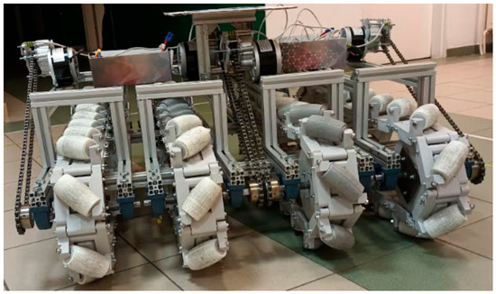
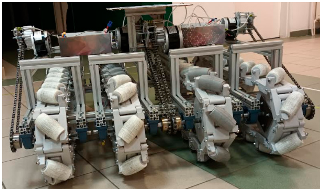
An alternative solution is provided by omnidirectional tracked mobile robots, which combine the maneuverability of omnidirectional motion with the inherent advantages of tracked locomotion. An example of such a vehicle is shown in Figure 1.
Figure 1.
Example of an omnidirectional tracked mobile robot.
Owing to their continuous contact with the supporting surface, tracked locomotion provides improved traction, enhanced load distribution, reduced ground pressure, and superior obstacle negotiation. These features render them highly effective for heavy-duty material handling, outdoor inspection, rescue operations, and other demanding applications that require both omnidirectional mobility and greater terrain adaptability [17]. Despite these advantages, the performance of an omnidirectional tracked robot is fundamentally governed by the complex interaction between its individual rollers and the supporting surface. The motion resistance generated at the roller–ground interface directly affects the driving torque requirements, energy consumption, traction characteristics, and overall dynamic behaviour. Consequently, accurate determination of longitudinal and lateral motion resistance constitutes an important prerequisite for drivetrain sizing, energy-efficient motion planning, and optimization of the robot’s mechanical design. Since the vehicle’s global behaviour originates from local contact at the roller level, understanding these interactions is essential for developing reliable design and modelling.
Over the past decade, numerous studies have addressed design challenges in omnidirectional mobility. Table 1 summarizes the representative literature in this field, considering locomotion type, level of analysis, used method, and primary research scope.
Table 1.
Summary of selected studies on the design of omnidirectional locomotion systems by locomotion type, level of analysis, methodology, and research scope.
A critical analysis of the literature reveals three major research gaps. First, existing studies focus overwhelmingly on wheeled configurations, leaving omnidirectional tracked robots considerably less investigated. Second, the majority of the research treats the robot as a complete macro-system rather than conducting a fundamental analysis of the mechanical behaviour at the level of individual components (e.g., the roller). Third, current modelling approaches rely primarily on computationally expensive physics-based models (e.g., full Multibody Dynamics), which are impractical for rapid iterative design or real-time control. In this context, surrogate models offer an alternative means of representing the response of computationally demanding simulations using simplified mathematical models. Their use has become increasingly common in robotics [33,34,35,36], particularly in applications that require repeated model evaluations, as they can substantially reduce computational time while maintaining satisfactory prediction accuracy.
Therefore, this study aims to develop computationally efficient surrogate models to determine the longitudinal and lateral motion resistance forces generated by an omnidirectional tracked roller as functions of its operating conditions and design parameters. First, a multibody dynamics model of a single roller is developed to reproduce the contact interaction between the roller and the supporting surface under different loading conditions, orientation angles, ground surface types, and bearing types. The numerical model is subsequently validated experimentally. The validated simulation model is then used to generate a comprehensive dataset describing the influence of selected design and operating parameters on motion resistance. Finally, multiple regression models are developed to provide a rapid determination of the resistance forces and to support the design process of omnidirectional tracked mobile robots. The main contributions of this study are the following:
- Development and experimental validation of a multibody dynamics model of an omnidirectional tracked roller for motion resistance determination;
- Quantitative identification of the influence of orientation angle, applied mass, surface type (through coefficient of friction consideration), and bearing type (through bearing friction torque consideration) on longitudinal and lateral motion resistance;
- Formulation of computationally efficient surrogate models that enable rapid determination of motion resistance forces to directly support the design and real-time control of omnidirectional tracked mobile robots.
2. Materials and Methods
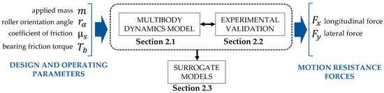
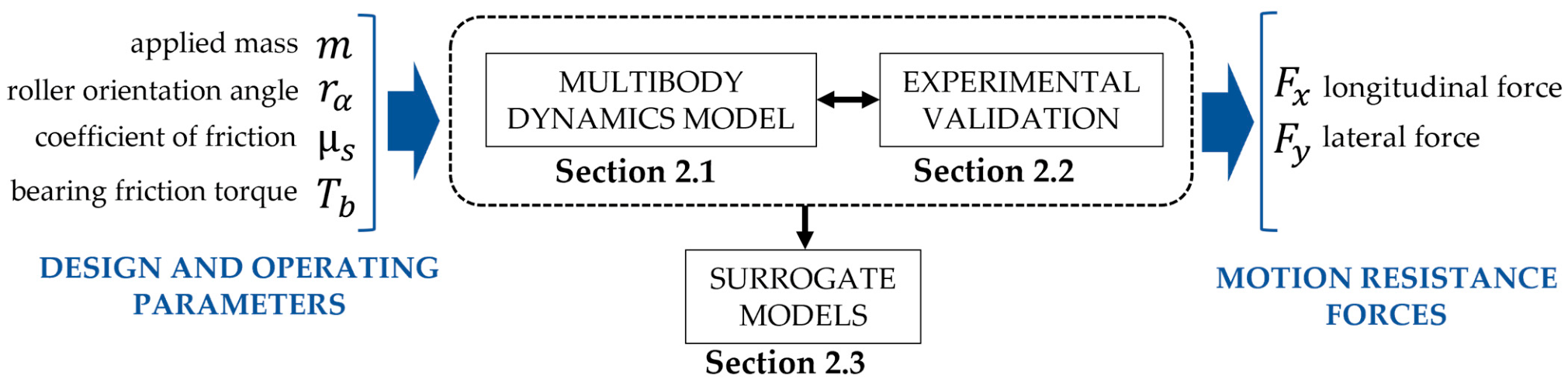
The adopted methodology combines physics-based modelling with data-driven surrogate modelling. A multibody dynamics model is first established to reproduce the roller–ground interaction and experimentally validated to ensure its predictive capability. The validated model is subsequently used to generate simulation data covering different combinations of design and operating parameters, which serve as the basis for constructing surrogate models of motion resistance. The overall workflow is summarized in Figure 2.
Figure 2.
Workflow of the proposed methodology.
2.1. Multibody Dynamics Model of Motion Resistance
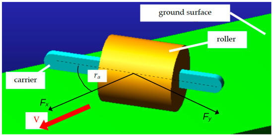
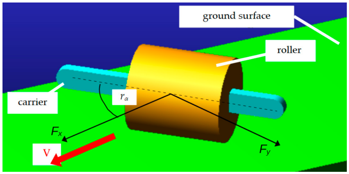
To investigate the motion resistance of the omni-track roller under various operating conditions, a three-dimensional multibody dynamics (MBD) model was developed in Hexagon Adams 2022. The model reproduces the rolling-sliding interaction between the roller and the ground surface, allowing the motion resistance forces (Fx and Fy) to be determined for different combinations of applied mass m, roller orientation angle rα (the angle between the roller’s rotational axis and the velocity vector), ground surface type (through coefficient of friction µ consideration), and bearing type (through bearing friction torque Tb consideration).
The numerical model consists of three rigid bodies: a fixed ground surface, the investigated omni-track roller, and a roller carrier to which the roller is connected through a frictionless revolute joint (Figure 3). The revolute joint allows free rotation of the roller about its longitudinal axis while constraining all other relative motions.
Figure 3.
Multibody dynamics model representation in Adams.
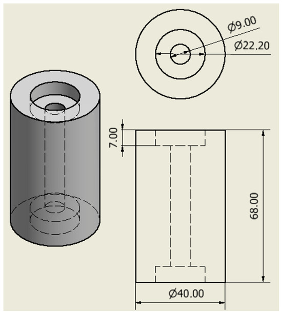
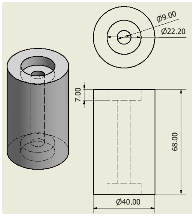
A cylindrical roller geometry was considered in the simulations with a diameter of 40 mm and a height of 68 mm. The geometry of the investigated roller is shown in Figure 4.
Figure 4.
3D model and technical drawing of the investigated omni-track roller (dimensions in mm).
The model is defined in a global Cartesian coordinate system. The roller carrier is prescribed to move at a constant velocity along the global X-axis, representing the robot’s translational motion. Lateral translation along the Y-axis is constrained, whereas vertical translation along the Z-axis remains unconstrained, allowing the roller to adjust its vertical position in response to the applied mass and contact forces. Rotations about the X- and Y-axes are constrained, while the rotation about the Z-axis defines the roller orientation angle rα with respect to the direction of motion.
The interaction between the roller and the ground surface is modelled using the Contact Force formulation available in the simulation environment. This contact model accounts for normal contact stiffness and damping, as well as friction, thereby reproducing rolling and sliding phenomena at the roller–ground interface. The contact parameters adopted in the simulations are summarized in Table 2.
Table 2.
Contact parameters used in the multibody dynamics model.
The coefficient of friction between the roller and the ground surface is treated as a variable simulation parameter to account for different surface conditions. Values of 0.60, 0.65, and 0.70 were selected to represent relatively high-friction contact conditions that may occur for elastomeric rollers operating on dry, relatively rough surfaces, such as concrete, asphalt, or textured industrial flooring.
The normal load acting on the roller is controlled by the applied mass, while the roller orientation angle varies to represent different design and operating conditions. In addition, the bearing friction torque is introduced via the revolute joint and varies with the investigated bearing type. Four torque levels were considered to represent different levels of bearing resistance associated with the sealing configuration. A value of 0.2 Nmm was assigned to an open bearing, while 1 Nmm was used for a metal-shielded bearing (ZZ). For sealed bearings with contact rubber seals (2RS), two friction torque levels were considered: 3 Nmm for a light seal contact and 6 Nmm for a higher seal contact pressure. The simulation input parameters and their ranges of investigation are summarized in Table 3.
Table 3.
Simulation input parameters.
For each combination of applied mass, roller orientation angle, coefficients of friction, and bearing friction torque, the model was simulated over a prescribed translational distance of 5 mm at a constant velocity of 10 mm/s.
2.2. Test Stand for the Experimental Validation of the Physical Model
Experimental tests were conducted to validate the developed multibody dynamics model and to assess its ability to reproduce the longitudinal and lateral motion resistance forces. The experiments were performed under controlled laboratory conditions. Three applied mass levels (0.385 kg, 0.65 kg, and 0.915 kg) and five roller orientation angles, ranging from 15° to 75° in 15° increments, were investigated.
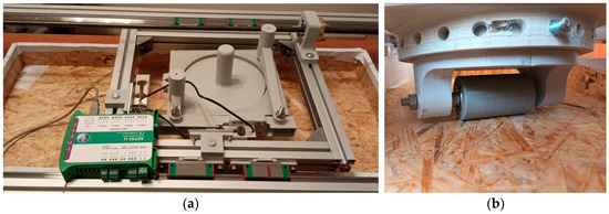
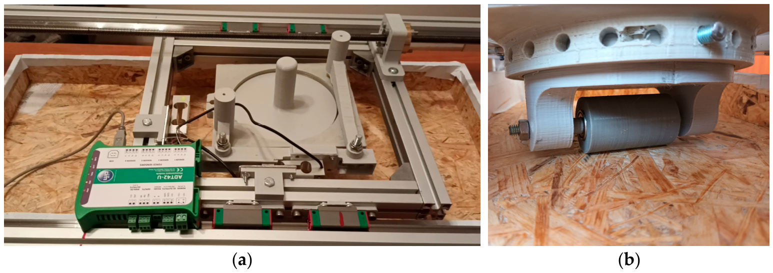
The experiments were conducted using a test stand (Figure 5) that enabled simultaneous measurement of the longitudinal force, acting along the direction of motion, and the lateral force, acting perpendicular to the direction of motion, generated during the translation of a passive roller over the ground surface.
Figure 5.
Top (a) and side (b) view of the developed test stand.
The measuring system consists of a linearly moving aluminum frame driven by a lead screw and guided by linear guides. The frame provides a maximum measurement distance of 400 mm and a maximum translational velocity of 20 mm/s. The longitudinal and lateral forces are measured using strain-gauge force sensors. An MAVIN NS6 sensor (produced by Hope Technologic (Xiamen) Co., Ltd., Xiamen, China) with a measurement range of 0–6 N is used to measure the longitudinal force, while an MAVIN NA27 sensor (produced by Hope Technologic (Xiamen) Co., Ltd., Xiamen, China) with a measurement range of 0–20 N is used to measure the lateral force. The signals from both sensors are acquired using an ADT42-U measuring unit (produced by WObit, Pniewy, Poland) at a sampling frequency of 80 Hz.
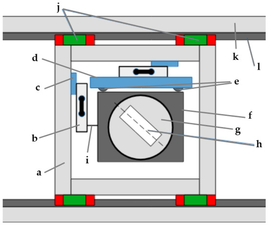
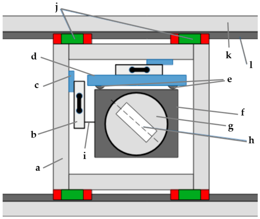
A measuring carriage is connected to the longitudinal strain-gauge sensor via an inextensible cable. The carriage contains the roller under test and the applied mass and is designed to allow adjustment of the roller orientation angle. A schematic representation of the test stand and its main components is presented in Figure 6.
Figure 6.
Schematic representation of the test stand: (a) aluminum frame, (b) strain-gauge force sensors, (c) sensor mountings, (d) measuring arm, (e) bearings, (f) measuring carriage, (g) rotary table for adjusting the roller orientation angle, (h) investigated roller, (i) inextensible cable, (j) linear guide carriages (k) aluminum frame (l) linear guide rail.
To ensure that the measured forces reflected steady-state motion resistance rather than transient effects associated with the initiation of motion, data recorded during the initial acceleration phase were excluded from the analysis.
2.3. Surrogate Modelling
A multibody dynamics model provides an accurate determination of motion resistance but requires repeated numerical simulations for every combination of design and operating parameters. Such an approach becomes computationally demanding when large numbers of design variants must be evaluated. To enable rapid prediction of motion resistance while preserving satisfactory accuracy, surrogate modelling was employed.
In surrogate modelling, results from a computationally expensive model are used to construct a computationally efficient approximation, referred to as a surrogate model. The surrogate reproduces the relationship between the model inputs and the corresponding outputs while substantially reducing the computational effort required for subsequent predictions. This reduction in computational time and resources is one of the main advantages of surrogate modelling and makes it particularly useful for engineering problems involving complex and nonlinear systems [37,38].
The general procedure for constructing a surrogate model consists of three main stages [39]:
2.3.1. Data Preparation and Selection of the Modelling Approach
The first stage involves identifying the relevant input variables, defining their ranges, and generating a set of input-output observations that adequately represents the investigated design space. Based on the characteristics of the investigated problem, an appropriate surrogate modelling approach is then selected. Surrogate modelling methods can be broadly divided into polynomial-based and machine learning-based approaches [40].
In this study, the input variables correspond to the design and operating parameters summarized in Table 3. Since the motion resistance is characterized by two response variables, namely the longitudinal force and the lateral force, two independent surrogate models were developed.
Among the various modelling techniques, Polynomial Response Surface (PRS) models were selected due to their simple mathematical formulation, low computational cost, and straightforward interpretation of the influence of individual input variables on the response [41]. In addition, PRS models provide explicit analytical equations that can be directly implemented in design optimization and real-time control algorithms.
The PRS employs regression analysis to establish the relationship between input variables and responses. The general form of a PRS model can be expressed as follows [42]:
where ε represents statistical error, xi denotes the i-th predictor variable, and β are the regression coefficients determined during the model fitting process.
The above formulation represents the surrogate as a linear combination of polynomial functions of the input variables, with linear and quadratic terms being most commonly used in the PRS approach.
2.3.2. Parameter Estimation and Model Fitting
In the second stage, the parameters of the selected surrogate model are estimated using the generated data. Given the selection of a polynomial response surface as the modelling approach, the model parameters were estimated using the ordinary least squares method [38] in Gretl 2022 software.
2.3.3. Model Testing
Finally, the model is tested on data not used during fitting to assess its predictive capability and verify its accuracy. The model performance is evaluated by comparing its predictions with the corresponding results of the original computational model using the adjusted coefficient of determination () and error metrics, including the mean absolute error (MAE), root mean square error (RMSE), and mean absolute percentage error (MAPE), defined as follows [42,43]
where x—actual values, y—predicted values, p—number of predictors, and n—number of observations.
To assess the predictive capability of the surrogate models, the complete MBD dataset was divided into a model-development dataset and an independent validation dataset. Rather than applying a random split, the validation set was defined by a combination of operating conditions that was not used during model estimation. The model-development dataset comprised 3240 simulation cases corresponding to all 90 investigated orientation angles and six mass levels, combined with two friction coefficients (μ = 0.6 and 0.65) and three bearing friction torque levels (0.2, 1, and 3 Nmm). The independent validation dataset comprised 540 cases covering the same range of orientation angles and mass levels, but with the friction coefficient and bearing friction torque simultaneously set to values excluded from model estimation, namely µ = 0.7 and Tb = 6 Nmm. This resulted in a validation set representing an unseen combination of operating conditions rather than a random subset of the simulation data. This approach was adopted to evaluate whether the surrogate models could generalize to previously unseen combinations of friction and bearing friction torque while retaining coverage of the full ranges of the investigated roller orientation angles and applied masses.
3. Results
The results obtained are presented in three stages, following the workflow adopted in the methodology. First, the results of the multibody dynamics simulations are presented, focusing on how the considered design and operating parameters affect the motion resistance of the omni-track roller. Next, the numerical model is experimentally validated using laboratory measurements obtained under selected operating conditions. Finally, based on the simulation results, surrogate models are developed to represent the motion resistance as a function of the investigated parameters.
3.1. Multibody Dynamics Simulation Results
The multibody dynamics model was used to investigate the influence of roller orientation angle, applied mass, bearing friction torque, and friction coefficient on the motion resistance of the omni-track roller. The simulations were performed for roller orientation angles ranging from 0° to 89° in 1° increments, six applied mass levels, four bearing friction torque variants, and three coefficients of friction. In total, 6480 simulation cases were analyzed, corresponding to all combinations of the investigated parameters. The complete simulation campaign required approximately five hours of computation.
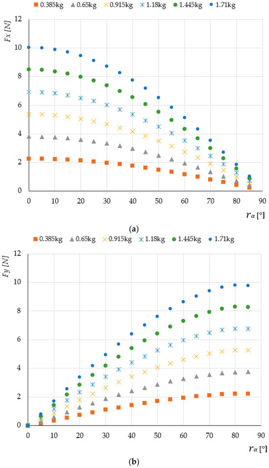
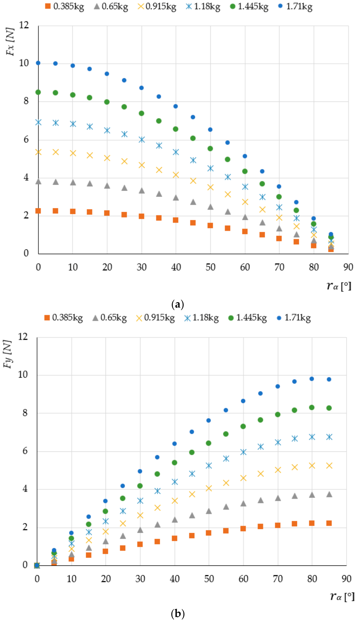
Figure 7 presents the variation in longitudinal and lateral resistance forces as a function of the roller orientation angle for different applied mass levels, using a bearing friction torque of 1 Nmm and a friction coefficient of 0.6.
Figure 7.
Influence of roller orientation angle on (a) longitudinal force Fx and (b) lateral force Fy for different applied masses (on the example of a bearing friction torque of 1 Nmm and a friction coefficient of 0.6).
As the orientation angle increases, the longitudinal resistance force decreases continuously, whereas the lateral resistance force increases. The opposite trends of Fx and Fy indicate that the orientation angle primarily determines the distribution of the resistance force between the longitudinal and lateral directions. The dependence on the orientation angle is clearly non-linear. The decrease in Fx and increase in Fy are not proportional to the angle itself, indicating that a linear representation of rα would not adequately describe the observed behaviour. The trends are consistent with the geometric decomposition of the resistance force into longitudinal and lateral components. In particular, the longitudinal and lateral components exhibit behaviour qualitatively corresponding to the cos(rα) and sin(rα) functions, respectively. These trends can be explained by the change in the direction of the contact reaction as the roller orientation angle increases. A larger orientation angle reduces the longitudinal component of the contact force while increasing its lateral component, resulting in a progressive redistribution of the resistance force between the Fx and Fy directions.
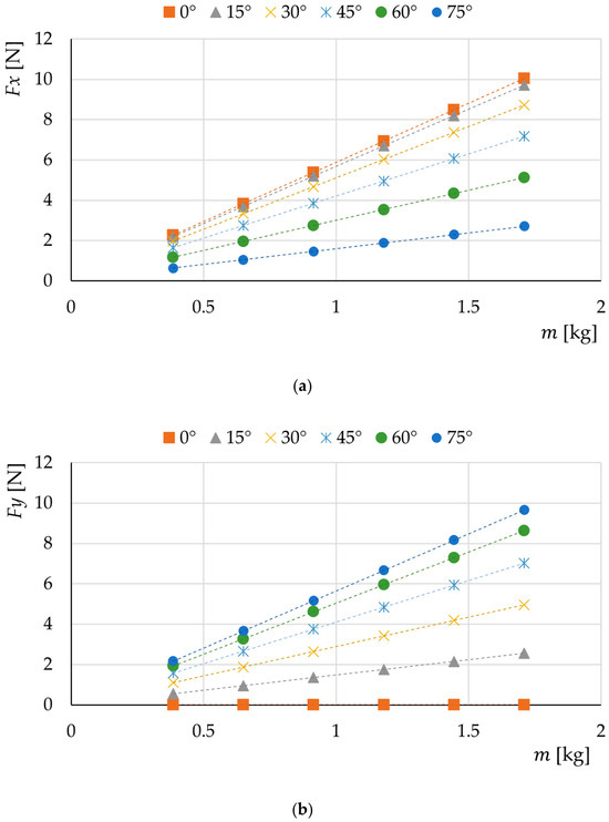
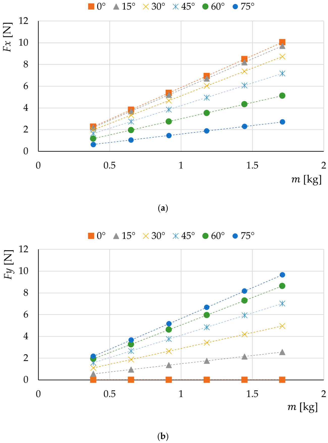
In addition to the angular dependence, both resistance force components increased with applied mass. For a given roller orientation angle, higher applied masses resulted in higher values of both Fx and Fy (Figure 8). The only exception occurred at a roller orientation angle of 0°, where the lateral force was zero regardless of the applied load, due to the absence of a lateral component of the contact force. The increase was approximately linear over the investigated range of applied masses. This behaviour was observed across the investigated angular range, although the magnitude of each force component depended strongly on the roller’s orientation angle. Thus, the applied mass primarily affected the magnitude of the resistance force, whereas the orientation angle determined its distribution between the longitudinal and lateral directions.
Figure 8.
Effect of applied mass on the motion resistance force components: (a) longitudinal force Fx; (b) lateral force Fy. Symbols represent simulation results, and dashed lines indicate linear trend lines.
The observed linear dependence arises from the adopted Coulomb friction model, in which the contact force is proportional to the normal reaction force. Consequently, increasing the applied mass proportionally increases the longitudinal and lateral force components, while the roller orientation angle determines the distribution of the motion resistance force between its longitudinal Fx and lateral Fy components. At a roller orientation angle of 0°, the contact force acts exclusively in the longitudinal direction, resulting in a zero lateral force component. The combined effect of applied mass and roller orientation angle indicates that their effects cannot be considered completely independently. An increase in applied mass scales the magnitude of the resistance force, while the orientation angle determines the proportion of this force acting in the longitudinal and lateral directions.
The coefficient of friction also exhibited a systematic influence on the resistance forces. Increasing the friction coefficient resulted in an approximately proportional increase in the force components for a given applied mass and roller orientation angle. This effect is consistent with the frictional nature of the contact resistance, for which the magnitude of the friction force depends on both the applied mass and the coefficient of friction.
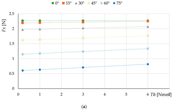
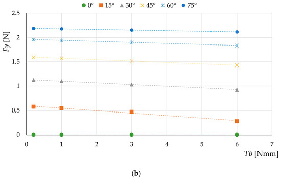
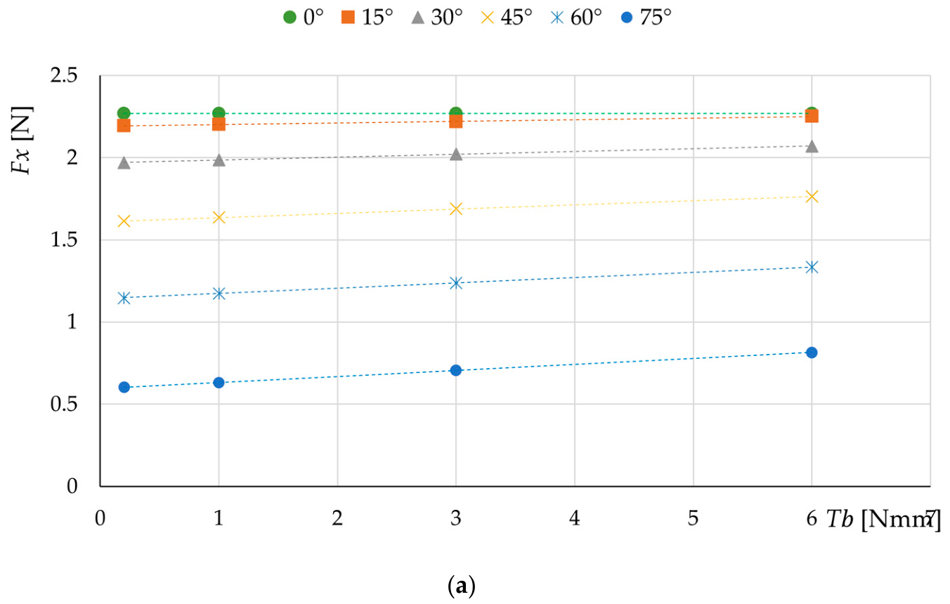
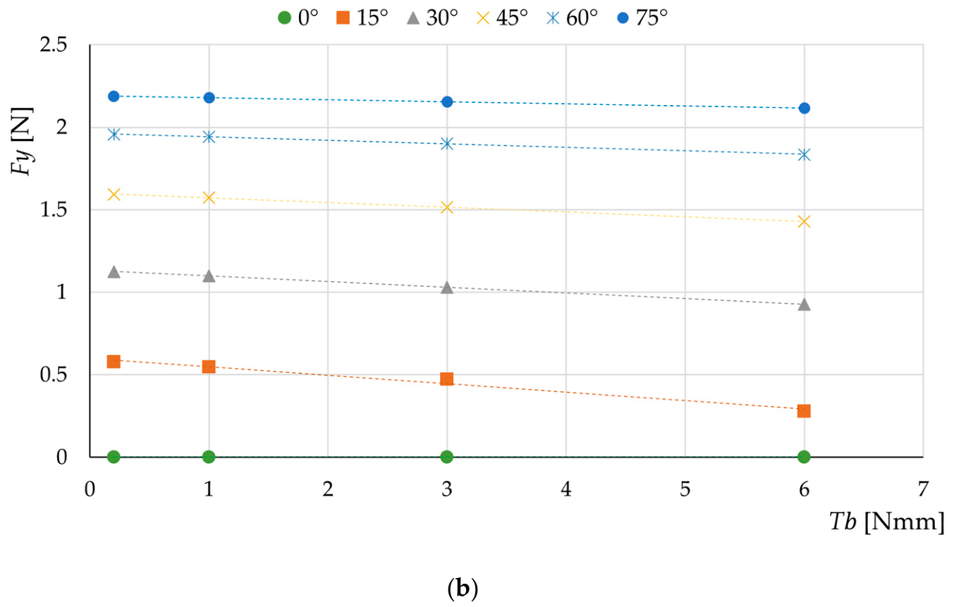
The bearing friction torque also affected the predicted motion resistance (Figure 9), although its contribution was substantially smaller than that associated with the applied mass and friction coefficient. For a given orientation angle, changes in bearing friction torque resulted in systematic changes in both force components. Importantly, the effect of bearing friction torque also depended on the roller orientation angle, indicating that its contribution to longitudinal and lateral resistance should be considered alongside the angular transformation.
Figure 9.
Influence of bearing friction torque on (a) longitudinal force Fx and (b) lateral force Fy for different roller orientation angles (on the example of applied mass 0.385 kg and a friction coefficient of 0.6). Symbols represent simulation results, and dashed lines indicate linear trend lines.
The preliminary analysis of the MBD results, therefore, identified two distinct groups of effects. The applied mass, coefficient of friction, and bearing friction torque primarily influenced the magnitude of the resistance forces, whereas the roller orientation angle governed their distribution between the longitudinal and lateral directions. The angular dependence was non-linear and was qualitatively consistent with cosine and sine functions for Fx and Fy, respectively. Moreover, the results indicated that the effects of applied mass and friction coefficient should be considered jointly, as their combined contribution determines the magnitude of the contact resistance. These observations were used to define the functional form of the subsequent surrogate models. Prior to this stage, the multibody dynamics model was experimentally validated to verify its accuracy.
3.2. Experimental Validation Results
To validate the developed multibody dynamics model, the simulation results were compared with the measurements obtained using the test stand described in Section 2.2. The numerical model was configured to reproduce the experimental conditions by considering five roller orientation angles (15°, 30°, 45°, 60°, and 75°) and three applied mass levels (0.385 kg, 0.65 kg, and 0.915 kg). The coefficient of friction between the roller and the ground surface was set to 0.6, based on the materials used in the experimental setup. Furthermore, the roller was modelled with bearings providing a constant friction torque of 1 Nmm, in accordance with the manufacturer’s specifications. A quantitative assessment of the numerical model accuracy was conducted based on the MAE, RMSE, and MAPE metrics determined for the Fx and Fy forces (Table 4).
Table 4.
Error metrics for the model validation.
The obtained mean absolute percentage errors (MAPE) were 11% for the longitudinal resistance force Fx and 8% for the lateral resistance force Fy, respectively. The mean absolute errors (MAE) did not exceed 0.24 N. The minor difference between the RMSE and MAE values confirms the absence of significant outliers and highlights the numerical stability of the developed model. The obtained metrics clearly demonstrate a high level of agreement between the model and experimental results, fully justifying its application to generate the dataset for surrogate modelling.
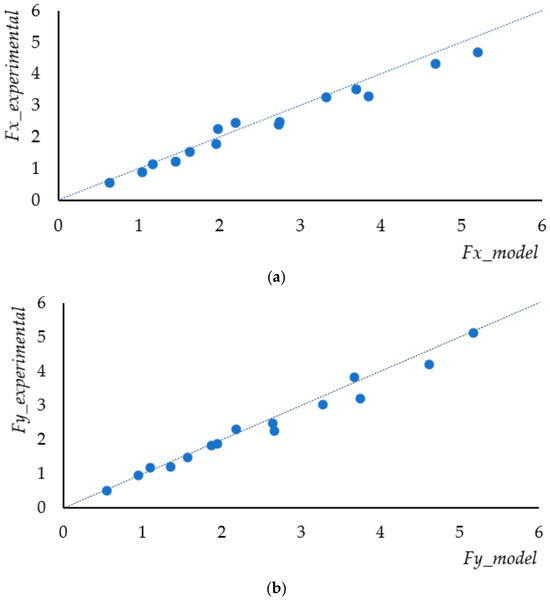
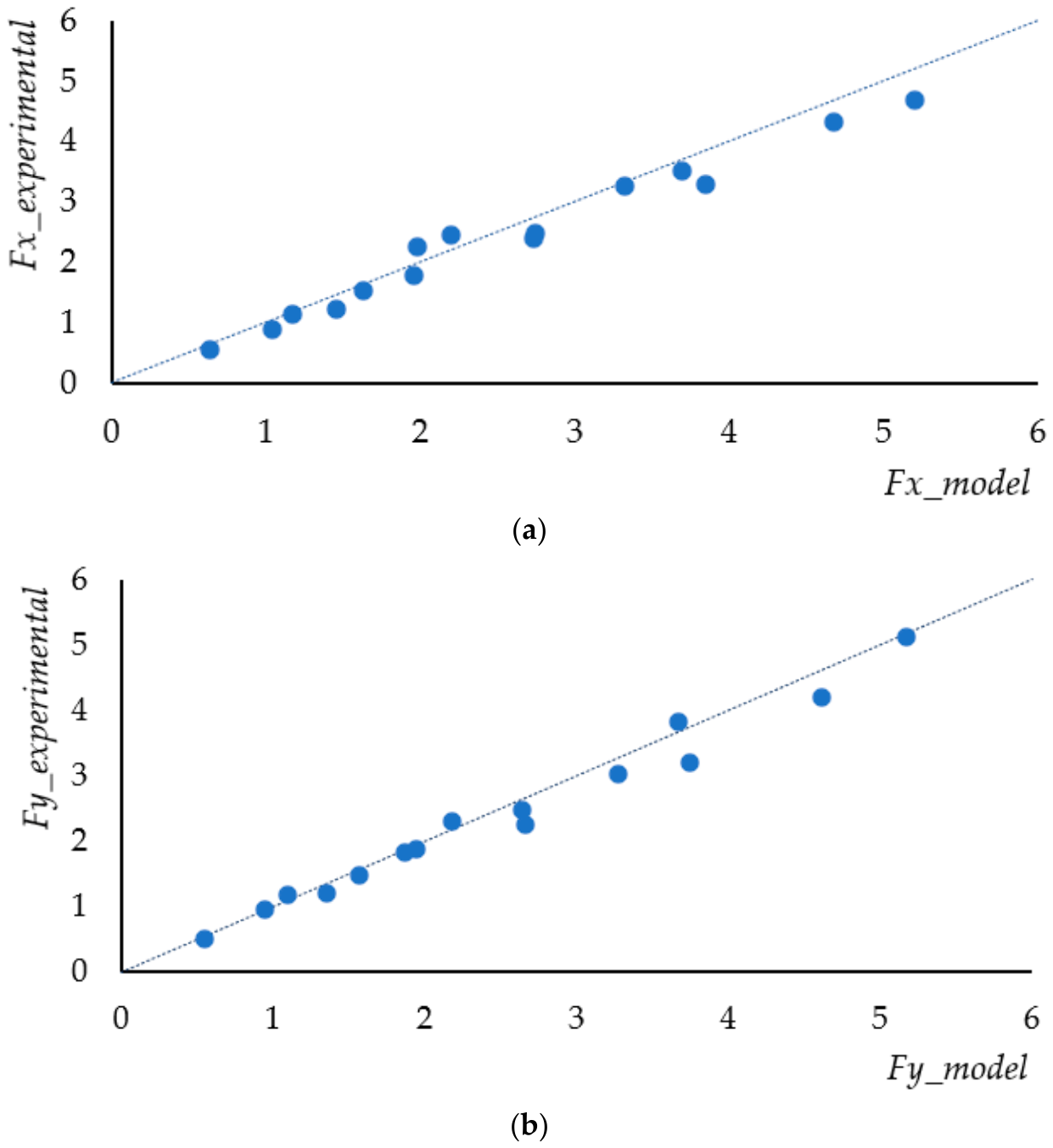
The scatter plots comparing the experimental and numerical model values for Fx and Fy demonstrate strong agreement across the analyzed operational range (Figure 10). The reference line represents the identity line (y = x), corresponding to ideal model accuracy.
Figure 10.
Scatter plots comparing experimental and numerical force values for: (a) longitudinal resistance force and (b) lateral resistance force. The dashed lines represent the lines of identity.
For both force components, the data points cluster tightly around the identity line, particularly in the low-to-medium force range (0–2.5 N), indicating high model accuracy. At higher load levels (>3 N), a slight systematic deviation is observed, with points lying marginally below the identity line. This reflects the model’s minor overestimation of forces, previously identified in the residual analysis. Overall, the minimal dispersion around the line of identity confirms a strong linear correlation between the model and physical measurements, validating the model for surrogate data generation.
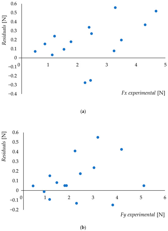
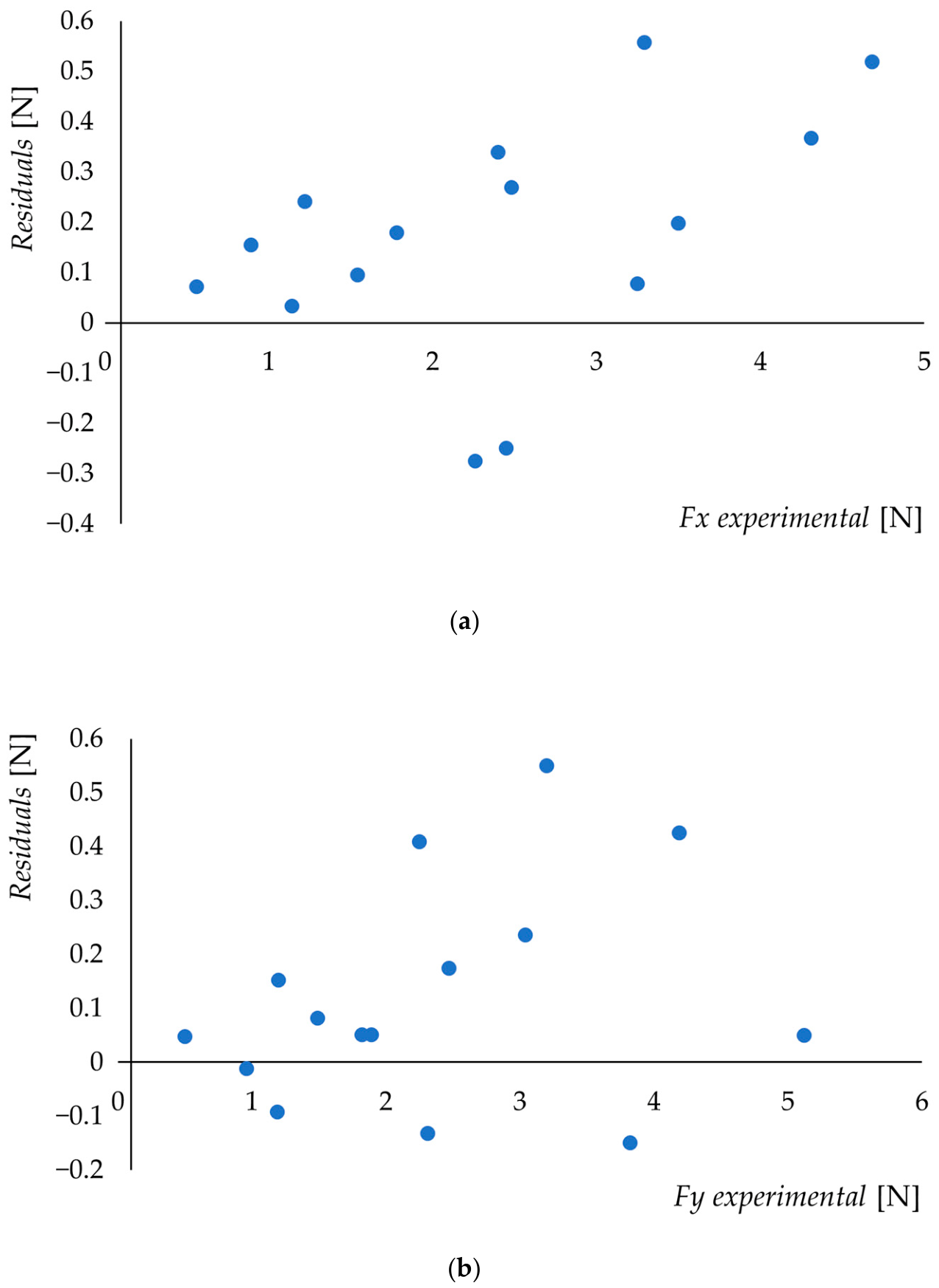
An analysis of the residual plots (Figure 11) for the longitudinal (Fx) and lateral (Fy) motion resistance forces reveals two key characteristics of the developed model. First, the positive sign of most residuals indicates a slight, systematic overestimation of force values by the model compared to experimental testing. Second, the residuals exhibit a proportional behaviour. Their absolute value increases with load, while the relative error remains constant (MAPE at 8–11%). This phenomenon stems from the idealization of contact geometry and the constant friction coefficient assumed in the simulation environment, whereas real-world conditions involve local micro-slip and nonlinear elastic deformations of the roller material.
Figure 11.
Residual plots (e = Fmodel − Fexperimental) as a function of experimental force values for: (a) longitudinal force Fx, and (b) lateral force Fy).
The results presented above confirm a high degree of agreement between the numerical model and the experimental data. Therefore, the validated model serves as a reliable tool for generating datasets to construct surrogate models.
3.3. Surrogate Motion Resistance Models
The surrogate modelling procedure comprised model development based on a dedicated subset of the MBD simulation data and subsequent model validation using independent MBD observations. Out of the total 6480 MBD simulation cases, comprising 12 parameter combinations of µ and Tb with 540 cases for each combination, 3780 cases were selected for surrogate modelling. Specifically, 3240 cases corresponding to six parameter combinations with µ values of 0.6 and 0.65 and Tb values of 0.2, 1 and 3 Nmm were used for model development, while 540 cases corresponding to the boundary combination of µ = 0.7 and Tb = 6 Nmm were reserved for independent validation of the model’s generalization capability. This parameter-based split was intentionally used instead of a conventional random split to assess the model’s ability to generalize to an unseen parameter combination at the boundary of the considered parameter domain, consistent with the rationale of boundary-aware data splitting discussed by [44].
3.3.1. Model Development
The surrogate models were developed using a dedicated subset of 3240 observations from the MBD simulation dataset, separated from the data used for subsequent model validation. Based on the relationships identified in the MBD simulations, two surrogate models were developed to predict the longitudinal and lateral motion resistance forces, Fx and Fy, respectively. Multiple linear regression was employed to construct the surrogate models.
The preliminary analysis presented in Section 3.1 indicated that the relationship between the roller orientation angle and the resistance forces was nonlinear. In particular, the variation of Fx and Fy with the roller orientation angle followed trends consistent with cosine- and sine-type dependencies, respectively. The analysis also indicated that the effect of the orientation angle should not be considered independently of the other model inputs, as the influence of the applied mass and friction coefficient changed with the roller orientation. Therefore, both nonlinear angular effects and interactions between the input variables were considered during model development. To account for the nonlinear angular dependence while retaining a linear regression framework, the roller orientation angle was transformed using the cosine function for the longitudinal force model and the sine function for the lateral force model. This transformation was motivated by the observed force decomposition: Fx decreased towards zero as the roller orientation angle approached 90°, whereas Fy increased towards its maximum. Accordingly, cos(rα) was used to represent the angular dependence of Fx, while sin(rα) was used for Fy.
In addition to the trigonometric transformation, interaction terms were introduced to account for the combined influence of the applied mass, friction coefficient, and roller orientation angle. As a conventional reference formulation, a linear regression model without interaction terms was also considered during the initial model development. Consistent with the relationships identified in Section 3.1, this formulation provided a substantially poorer fit to the MBD results, indicating that the effects of the input variables could not be adequately represented as independent contributions. For Fx, the model yielded = 0.89 with an RMSE of 0.93, while for Fy, = 0.88 and an RMSE of 0.95 were obtained. Introducing the trigonometric transformations without interaction terms improved these values to = 0.91 and 0.84 for Fx, and = 0.90 and 0.86 for Fy, respectively. Based on these results, for the longitudinal force, the transformed variables considered during model development included:
For the lateral force, the corresponding variables were defined as:
The functional forms defined in the equations above are derived from the kinematics and contact dynamics of the roller. The relative contact velocity is decomposed into a component along the passive roller axis, which leads to pure sliding, and an orthogonal component accommodated by passive rolling. According to Coulomb’s law of friction, the contact sliding force is proportional to the normal load and acts opposite to the slip vector. The cosine and sine functions arise from the projection of the slip-resisting force onto the longitudinal and lateral axes of the adopted coordinate system, respectively, as the direction of the slip vector changes with the roller orientation angle. This also gives rise to the interaction terms combining the applied mass and friction coefficient with the trigonometric orientation function. In contrast, the bearing friction torque operates through a distinct mechanism, acting via a tangential contact force directed opposite to the rolling direction. Because rolling is orthogonal to sliding, the corresponding force components are likewise dependent on the roller orientation angle.
The final model was obtained using the ordinary least-squares method combined with backward variable selection based on the statistical significance of the regression coefficients. At each step, the predictor with the highest p-value was removed, provided that its p-value exceeded the predefined significance level of 0.05. The procedure was repeated until all remaining predictors were statistically significant (p < 0.05). Equation (13) presents the surrogate model developed for predicting the longitudinal motion resistance Fx:
Fx = 0.135 − 0.172cos(rα) + 9.82mµcos(rα) + 0.024Tbcos(rα)
The model consists of an intercept and three physically interpretable terms. The first angular term, cos(rα), represents the direct contribution associated with the orientation of the roller. The mµcos(rα) term describes the combined effect of the applied mass and friction coefficient on the longitudinal resistance, while the Tbcos(rα) term represents the contribution of bearing friction torque projected onto the longitudinal direction. The positive coefficient of the mµcos(rα) term indicates that increasing either the applied mass or the friction coefficient increases the longitudinal resistance. The positive coefficient associated with bearing friction torque indicates an additional increase in Fx with increasing bearing friction torque. The intercept was retained to improve the numerical fit over the selected modelling domain of 0° ≤ rα ≤ 89°. At rα = 90°, Fx is physically near zero. However, this boundary point was excluded. Since 90° is outside this domain, the non-zero intercept should not be interpreted as a violation of the physical boundary condition at 90°.
The variables were used in their original physical units, as stated in Table 3. Accordingly, the intercept and the coefficient of cos(rα) have units of N, the coefficient of mµcos(rα) has units of N/kg, and the coefficient of Tbcos(rα) has units of mm−1.
Equation (14) presents the surrogate model developed for predicting the lateral motion resistance Fy:
Fy = 0.021sin(rα) + 9.69mµsin(rα) − 0.026Tbsin(rα)
The structure of the lateral force model is analogous to that of the longitudinal force model, but the cosine transformation is replaced by the sine transformation to reflect the opposite angular dependence of the two force components. The mµsin(rα) term represents the combined effect of the applied mass and friction coefficient on the lateral resistance, whereas Tbsin(rα) accounts for the contribution of bearing friction torque to the lateral force. In this model, the intercept term was omitted to satisfy the physical constraint that Fy = 0 N at rα = 0°. The constrained formulation also resulted in improved model fit compared with the unrestricted model, including an intercept. Thus, the physically constrained formulation was considered more appropriate for describing the lateral motion resistance.
The variables were used in their original physical units, as in the longitudinal motion resistance model. Accordingly, the intercept and the coefficient of sin(rα) have units of N, the coefficient of mµsin(rα) has units of N/kg, and the coefficient of Tbsin(rα) has units of mm−1.
Regression coefficients in both models were statistically significant at (p < 0.001) when evaluated using heteroskedasticity-consistent standard errors. The models also showed a very high goodness of fit to the development data. For the Fx model, = 0.999871, with a residual standard error of 0.031. For the Fy model, the corresponding values were = 0.9998, and a residual standard error of 0.05. Based on the F-test for overall model fit, the models were statistically significant for both Fx (F(3, 3236) = 12,944.825, p < 0.001) and Fy (F(3, 3237) = 12,605.867, p < 0.001).
Multicollinearity was assessed using variance inflation factors (VIF). The VIF values were low for both models, ranging from 1.261 to 2.238 for Fx and from 1.275 to 2.307 for Fy, indicating no substantial multicollinearity among the retained predictors. Residual diagnostics indicated statistically significant heteroskedasticity according to the Breusch–Pagan test (LM = 1422.439, p < 0.001 for Fx; LM = 744.792, p < 0.001 for Fy). This indicates that the residual variance was not constant across the investigated operating conditions. Therefore, heteroskedasticity-consistent HC1 standard errors were used for statistical inference. The Doornik–Hansen test rejected the null hypothesis of normally distributed residuals (χ2(2) = 221.199, p < 0.001 for Fx; χ2(2) = 541.593, p < 0.001 for Fy, which may be detected due to the large sample size. However, this deviation from normality does not substantially affect the adequacy of the models, as indicated by the very high values, low residual standard errors, and high overall statistical significance of the models.
The models were subsequently evaluated using the independent MBD observations excluded from model development. The results of the validation procedures are presented in Section 3.3.2.
3.3.2. Model Validation
The predictive performance of the developed surrogate models was evaluated using the remaining 540 MBD observations that were not included in the model development process. These observations represented combinations of operating conditions excluded from model fitting, including a different bearing friction torque and coefficient of friction from those used for model development. The previously estimated regression equations were applied directly to these observations without any further parameter estimation or model adjustment.
The validation results are summarized in Table 5.
Table 5.
Validation results of the surrogate models for longitudinal and lateral motion resistance forces.
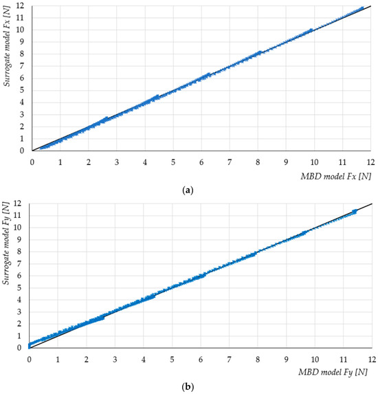
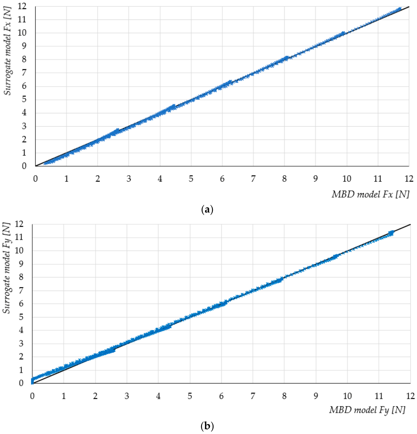
Both surrogate models showed a close agreement with the independent MBD results, with values exceeding 0.99. The model for Fx achieved a higher predictive accuracy, with an MAE of 0.087 N and an RMSE of 0.101 N, compared with 0.11 N and 0.137 N, respectively, for Fy. The maximum absolute residuals were 0.250 N for Fx and 0.338 N for Fy, indicating that the lateral force was more difficult to approximate than the longitudinal force. Nevertheless, the obtained values of 0.9989 for Fx and 0.9981 for Fy indicate that the surrogate models reproduced the variation in the corresponding MBD force components with high accuracy.
The validation results demonstrate a close agreement between the surrogate predictions and the independent MBD results for both force components. The slightly higher prediction errors observed for Fy indicate that the lateral force was more difficult to approximate than the longitudinal force, although the coefficient of determination remained above 0.99. The comparison between predicted and reference values is presented in Figure 12 as scatter plots, where the proximity of observations to the 1:1 line provides a visual assessment of prediction accuracy.
Figure 12.
Comparison of surrogate model predictions with MBD results for (a) longitudinal force and (b) lateral force.
The close clustering of the observations around the 1:1 line confirms the high agreement between the surrogate predictions and the independent MBD results.
4. Discussion
The results indicate that the proposed surrogate models provide a sufficiently accurate representation of the motion resistance predicted by the MBD model while substantially reducing the computational effort of repeated evaluations. The close agreement between the surrogate predictions and the independent MBD data used for their validation confirms that the proposed models can serve as a practical approximation of the motion resistance forces within the investigated operating range. The experimental results, in turn, confirm the adequacy of the MBD model under the selected representative conditions.
The developed models have direct potential for application in the design of mobile robotic platforms equipped with omnidirectional tracks. In particular, the predicted longitudinal resistance can be incorporated into the estimation of the required drive torque and motor power. The model can therefore support motor and drivetrain sizing by enabling evaluation of the resistance force under different roller orientations, loads, friction conditions, and bearing friction torque levels without repeatedly performing computationally expensive MBD simulations. The model can also support the selection and comparison of bearing solutions, as bearing friction torque constitutes an explicit input to the surrogate formulation. This may be particularly useful at the preliminary design stage, where many drivetrain configurations must be evaluated.
From a system design perspective, the model also enables consideration of the effects of individual design choices jointly. For example, reducing bearing friction torque may decrease the total motion resistance and consequently reduce the required drive torque, whereas changes in contact conditions or vehicle loading may have a substantially larger effect on the required driving force. The surrogate formulation, therefore, provides a computationally inexpensive means of assessing such design trade-offs before detailed mechanical design or full system simulation.
The low computational complexity of analytical surrogate models also enables their use in online control. Unlike an MBD model, the proposed equations require only a small number of arithmetic operations. This makes them suitable for implementation in embedded control systems, where computational resources and response time are limited. This computational advantage was also confirmed by a benchmark: the longitudinal-force equation required 29.61 ns per evaluation with direct trigonometric calculation and 13.88 ns with the trigonometric term precomputed, compared with more than 1 s for a single MBD simulation on the same computer. This corresponds to a speed-up of more than 34 million times and 72 million times, respectively.
The predicted longitudinal and lateral resistance could be incorporated into motion controllers to compensate for changes in roller orientation, payload, or estimated contact conditions. Such a model could potentially be used for feed forward compensation, torque allocation, or real-time estimation of the force demand associated with the omnidirectional drive. However, the applicability of the proposed models to online control should nevertheless be considered within the operating conditions investigated in this study. The present formulation was developed from simulations performed at a fixed velocity and does not explicitly account for acceleration, transient effects, or dynamically varying contact conditions. Therefore, although the low computational cost makes the models suitable for potential use as a feedforward resistance characteristic in real-time control, their application under transient operating conditions requires further validation. In this context, the motion resistance characterized in this study can be regarded as a state-dependent load disturbance acting on the drivetrain. Such disturbances can be addressed at the controller level using, for example, disturbance-rejection approaches based on state filtering and command-filtered backstepping [45], or learning-based approaches using an actor-critic mechanism [46]. These approaches address the online estimation and compensation of the aggregate effects of disturbances from measured system responses, whereas the present study characterizes one physical component of the motion resistance offline, before prototype-level implementation. The two approaches are therefore complementary: the proposed surrogate models can support early-stage drivetrain sizing and provide a physically interpretable feedforward term that may reduce the disturbance to be handled by feedback control. Their integration with disturbance-rejection or learning-based control strategies is left for future work.
Several limitations of the present study should be acknowledged. First, the models were developed for a single roller geometry and within a predefined range of operating conditions. The angular domain was limited to 0° ≤ rα ≤ 89°. Although the observed dependence of Fy on the orientation angle is well represented by the sine transformation within this range, the behaviour at exactly 90° is discontinuous, with the Fy resistance force dropping to zero. Consequently, the trigonometric formulation adopted in the present models should not be extrapolated to 90°, and the models should be regarded as valid only within the investigated angular range. Second, the investigation focused on a defined range of operating parameters. The experimental validation of the MBD model was performed for three mass levels, five roller orientation angles, one bearing friction torque level, and one coefficient of friction. Therefore, although the MBD model was validated against experimental measurements, the experimental validation did not cover the entire parameter space used for surrogate model development. The additional validation of the surrogate model was performed using independent MBD simulations and, therefore, primarily assessed its ability to reproduce the numerical model outside the training dataset. Finally, the present models do not explicitly account for parameters such as travelling velocity, acceleration, dynamic load transfer, surface irregularities, roller deformation, or changes in contact conditions during operation. These factors may become relevant when the model is transferred from controlled simulation conditions to a complete mobile robotic platform operating in realistic environments.
Future research should extend the proposed approach from an individual omni-track roller to the complete mobile robotic system. In a full-robot model, the interactions between multiple rollers, track geometry, load distribution, and the drive system could be considered simultaneously. Such an extension would allow the surrogate approach to be used not only for predicting the resistance of an individual roller but also for estimating the overall motion resistance and energy demand of the robotic platform. Further research could also investigate the influence of other drivetrain components and design parameters, including roller geometry, bearing characteristics, track material, contact stiffness, and surface properties. Extending the experimental campaign to a broader range of operating conditions would additionally enable more comprehensive validation of the surrogate models and assessment of their applicability under realistic operating scenarios. Ultimately, integrating such surrogate models with robot-level simulation and control frameworks could provide a computationally efficient link between mechanical design, energy aware motion planning, and real-time control of omnidirectional tracked robots.
5. Conclusions
This study presented a surrogate modelling approach for estimating the motion resistance forces of an omnidirectional tracked roller under varying operating conditions and design parameters. A multibody dynamics model was developed in Hexagon Adams to investigate the effects of roller orientation angle, applied mass, coefficient of friction, and bearing friction torque on the longitudinal and lateral force components. Based on the MBD simulation data, Polynomial Response Surface surrogate models were developed to provide a computationally efficient representation of the resistance forces. The surrogate models achieved a close agreement with the reference MBD results, demonstrating that the main relationships governing the force response can be captured without performing a full multibody simulation for each new combination of input parameters.
The proposed surrogate models provide a practical tool for rapid estimation of motion resistance during the preliminary design and analysis of omnidirectional tracked systems. Their use can facilitate repeated evaluations of different operating conditions and support the selection of drive and mechanical components without the computational cost associated with repeated MBD simulations. The approach can also serve as a basis for integrating resistance estimation into higher level robot design, optimization, and control.
Future research should extend the experimental validation to a broader range of operating conditions and investigate the applicability of the proposed approach to complete omnidirectional tracked robot systems.
The main contribution of the study is not only the development of the surrogate models, but also the demonstration that a computationally expensive MBD-based motion resistance analysis can be transformed into a fast predictive tool suitable for engineering applications.
Author Contributions
Conceptualization, M.F. and A.D.; methodology, M.F. and A.D.; software, M.F. and A.D.; validation, M.F.; formal analysis, M.F.; investigation, M.F.; resources, M.F.; data curation, M.F.; writing—original draft preparation, A.D.; writing—review and editing, A.D.; visualization, M.F. and A.D.; supervision, M.F.; project administration, M.F.; funding acquisition, A.D. All authors have read and agreed to the published version of the manuscript.
Funding
This research was funded by the Wroclaw University of Science and Technology, Faculty of Mechanical Engineering, Department of Technical Systems Operation and Maintenance, Poland (K53W10).
Institutional Review Board Statement
Not applicable.
Informed Consent Statement
Not applicable.
Data Availability Statement
The original contributions presented in the study are included in the article, further inquiries can be directed to the corresponding authors.
Conflicts of Interest
The authors declare no conflicts of interest.
Abbreviations
The following abbreviations are used in this manuscript:
| MBD | multibody dynamics simulation |
| PRS | Polynomial Response Surface |
| MAE | mean absolute error |
| RMSE | root mean square error |
| MAPE | mean absolute percentage error |
| VIF | Variance Inflation Factor |
References
- Raj, R.; Kos, A. A Comprehensive Study of Mobile Robot: History, Developments, Applications, and Future Research Perspectives. Appl. Sci. 2022, 12, 6951. [Google Scholar] [CrossRef] [Scilit]
- Li, P.; Wei, L.; Wu, D. An Intelligently Enhanced Ant Colony Optimization Algorithm for Global Path Planning of Mobile Robots in Engineering Applications. Sensors 2025, 25, 1326. [Google Scholar] [CrossRef] [Scilit]
- Giel, R.; Werbińska-Wojciechowska, S.; Malewicz, J. Autonomous Mobile Robot Navigation Issues in Terms of Obstacles Detection in Disrupting Operating Conditions—Case Study. In Proceedings of the Reliability and Statistics in Transportation and Communication; Springer: Cham, Switzerland, 2023. [Google Scholar]
- Werbińska-Wojciechowska, S.; Giel, R.; Winiarska, K. Digital Twin Approach for Operation and Maintenance of Transportation System—Systematic Review. Sensors 2024, 24, 6069. [Google Scholar] [CrossRef] [Scilit]
- Giel, R.; Werbińska-Wojciechowska, S.; Winiarska, K. Employing Digital Twins in Operation and Maintenance Management of Transportation Systems. In Proceedings of the Lecture Notes in Intelligent Transportation and Infrastructure; Springer: Cham, Switzerland, 2024. [Google Scholar]
- Alemu, Y.; Szrek, J. Locomotion of Tensegrity Robot through Bar-Length Modulation: Simulation and Dynamic Analysis. Arch. Mech. Eng. 2025, 72, 741–764. [Google Scholar] [CrossRef] [Scilit]
- Poskart, B.; Iskierka, G.; Krot, K.; Burduk, R.; Gwizdal, P.; Gola, A. Multi-Parameter Predictive Model of Mobile Robot’s Battery Discharge for Intelligent Mission Planning in Multi-Robot Systems. Sensors 2022, 22, 9861. [Google Scholar] [CrossRef] [Scilit]
- Sperzyński, P.; Bałchanowski, J. Dimensional Synthesis of Suspension System of Wheel-Legged Mobile Robot. J. Theor. Appl. Mech. 2025, 63, 633–644. [Google Scholar] [CrossRef] [Scilit]
- Ding, T.; Zhang, Y.; Ma, G.; Cao, Z.; Zhao, X.; Tao, B. Trajectory Tracking of Redundantly Actuated Mobile Robot by MPC Velocity Control under Steering Strategy Constraint. Mechatronics 2022, 84, 102779. [Google Scholar] [CrossRef] [Scilit]
- Taheri, H.; Zhao, C.X. Omnidirectional Mobile Robots, Mechanisms and Navigation Approaches. Mech. Mach. Theory 2020, 153, 103958. [Google Scholar] [CrossRef] [Scilit]
- Azizi, M.R.; Rastegarpanah, A.; Stolkin, R. Motion Planning and Control of an Omnidirectional Mobile Robot in Dynamic Environments. Robotics 2021, 10, 48. [Google Scholar] [CrossRef] [Scilit]
- Ishigami, G.; Iagnemma, K.; Overholt, J.; Hudas, G. Design, Development, and Mobility Evaluation of an Omnidirectional Mobile Robot for Rough Terrain. J. Field Robot. 2015, 32, 880–896. [Google Scholar] [CrossRef] [Scilit]
- Hijikata, M.; Miyagusuku, R.; Ozaki, K. Wheel Arrangement of Four Omni Wheel Mobile Robot for Compactness. Appl. Sci. 2022, 12, 5798. [Google Scholar] [CrossRef] [Scilit]
- Li, Y.; Dai, S.; Zheng, Y.; Tian, F.; Yan, X. Modeling and Kinematics Simulation of a Mecanum Wheel Platform in RecurDyn. J. Robot. 2018, 2018, 9373580. [Google Scholar] [CrossRef] [Scilit]
- Gfrerrer, A. Geometry and Kinematics of the Mecanum Wheel. Comput. Aided Geom. Des. 2008, 25, 784–791. [Google Scholar] [CrossRef] [Scilit]
- Tagliavini, L.; Colucci, G.; Botta, A.; Cavallone, P.; Baglieri, L.; Quaglia, G. Wheeled Mobile Robots: State of the Art Overview and Kinematic Comparison Among Three Omnidirectional Locomotion Strategies. J. Intell. Robot. Syst. 2022, 106, 57. [Google Scholar] [CrossRef] [Scilit]
- Bruzzone, L.; Nodehi, S.E.; Fanghella, P. Tracked Locomotion Systems for Ground Mobile Robots: A Review. Machines 2022, 10, 648. [Google Scholar] [CrossRef] [Scilit]
- Zhang, Y.; Huang, T. Research on a Tracked Omnidirectional and Cross-Country Vehicle. Mech. Mach. Theory 2015, 87, 18–44. [Google Scholar] [CrossRef] [Scilit]
- Mortensen Ernits, R.; Hoppe, N.; Kuznetsov, I.; Uriarte, C.; Freitag, M. A New Omnidirectional Track Drive System for Off-Road Vehicles. In Proceedings of the XXII International Conference MHCL’17, Belgrade, Serbia, 4–6 October 2017. [Google Scholar]
- Fang, Y.; Zhang, Y.; Li, N.; Shang, Y. Research on a Medium-Tracked Omni-Vehicle. Mech. Sci. 2020, 11, 137–152. [Google Scholar] [CrossRef] [Scilit]
- Fiedeń, M.; Bałchanowski, J. A Mobile Robot with Omnidirectional Tracks—Design and Experimental Research. Appl. Sci. 2021, 11, 11778. [Google Scholar] [CrossRef] [Scilit]
- Fiedeń, M. Kinematic Analysis of an Omnidirectional Tracked Vehicle. Appl. Sci. 2025, 15, 6111. [Google Scholar] [CrossRef] [Scilit]
- Fiedeń, M.; Bałchanowski, J. Simulation Studies and Experimental Research of Omnidirectional Tracked Vehicle. J. Theor. Appl. Mech. 2024, 62, 337–348. [Google Scholar] [CrossRef] [Scilit]
- Wang, C.; Liu, X.; Yang, X.; Hu, F.; Jiang, A.; Yang, C. Trajectory Tracking of an Omni-Directional Wheeled Mobile Robot Using a Model Predictive Control Strategy. Appl. Sci. 2018, 8, 231. [Google Scholar] [CrossRef] [Scilit]
- Yepez-Figueroa, J.J.; Victores, J.G.; Oña, E.D.; Balaguer, C.; Jardón, A. Design and Development of an Omnidirectional Three-Wheeled Industrial Mobile Robot Platform. Appl. Sci. 2025, 15, 5277. [Google Scholar] [CrossRef] [Scilit]
- Doroftei, I.; Grosu, V.; Spinu, V. Omnidirectional Mobile Robot–Design and Implementation. In Bioinspiration and Robotics Walking and Climbing Robots; Habib, M.K., Ed.; I-Tech Education and Publishing: Vienna, Austria, 2007; ISBN 978-3-902613-15-8. [Google Scholar]
- Bernardo, R.; Sousa, J.M.C.; Botto, M.A.; Gonçalves, P.J.S. A Novel Control Architecture Based on Behavior Trees for an Omni-Directional Mobile Robot. Robotics 2023, 12, 170. [Google Scholar] [CrossRef] [Scilit]
- Qian, J.; Zi, B.; Wang, D.; Ma, Y.; Zhang, D. The Design and Development of an Omni-Directional Mobile Robot Oriented to an Intelligent Manufacturing System. Sensors 2017, 17, 2073. [Google Scholar] [CrossRef] [Scilit]
- Palacín, J.; Martínez, D.; Rubies, E.; Clotet, E. Suboptimal Omnidirectional Wheel Design and Implementation. Sensors 2021, 21, 865. [Google Scholar] [CrossRef] [Scilit]
- Neaz, A.; Lee, S.; Nam, K. Design and Implementation of an Integrated Control System for Omnidirectional Mobile Robots in Industrial Logistics. Sensors 2023, 23, 3184. [Google Scholar] [CrossRef] [Scilit]
- Rojas-López, A.G.; Villarreal-Cervantes, M.G.; Rodríguez-Molina, A.; Paredes-Ballesteros, J.A. Efficient Online Controller Tuning for Omnidirectional Mobile Robots Using a Multivariate-Multitarget Polynomial Prediction Model and Evolutionary Optimization. Biomimetics 2025, 10, 114. [Google Scholar] [CrossRef] [Scilit]
- Duda, S.; Gembalczyk, G.; Machoczek, T.; Kowalik, Z. Experimental Evaluation of Rolling Resistance in Omnidirectional Wheels Under Quasi-Static Conditions. Sensors 2025, 25, 5026. [Google Scholar] [CrossRef] [Scilit]
- Bold, L.; Rosenfelder, M.; Eschmann, H.; Ebel, H.; Worthmann, K. On Koopman-Based Surrogate Models for Non-Holonomic Robots. IFAC-Pap. 2024, 58, 55–60. [Google Scholar] [CrossRef] [Scilit]
- Zargar, S.H.; Brown, N.C. Predicting Robotic Constructability in Early Design of a Panelized Structure: A Surrogate Model for a Mobile Robotic Arm. Proc. IASS Annu. Symp. 2024, 2024, 1–10. [Google Scholar]
- Yin, J.; Hu, Z.; Mourelatos, Z.P.; Gorsich, D.; Singh, A.; Tau, S. Efficient Reliability-Based Path Planning of Off-Road Autonomous Ground Vehicles Through the Coupling of Surrogate Modeling and RRT*. IEEE Trans. Intell. Transp. Syst. 2023, 24, 15035–15050. [Google Scholar] [CrossRef] [Scilit]
- Hsiao, J.C.; Shivam, K.; Chou, C.L.; Kam, T.Y. Shape Design Optimization of a Robot Arm Using a Surrogate-Based Evolutionary Approach. Appl. Sci. 2020, 10, 2223. [Google Scholar] [CrossRef] [Scilit]
- Yarmohammadian, R.; Put, F.; Van Coile, R. Physics-Informed Surrogate Modelling in Fire Safety Engineering: A Systematic Review. Appl. Sci. 2025, 15, 8740. [Google Scholar] [CrossRef] [Scilit]
- Kudela, J.; Matousek, R. Recent Advances and Applications of Surrogate Models for Finite Element Method Computations: A Review. Soft Comput. 2022, 26, 13709–13733. [Google Scholar] [CrossRef] [Scilit]
- Forrester, A.I.J.; Sóbester, A.; Keane, A.J. Engineering Design via Surrogate Modelling: A Practical Guide, 1st ed.; Wiley: Hoboken, NJ, USA, 2008; ISBN 978-0-470-06068-1. [Google Scholar]
- Liu, L.; Li, Z.; Kang, H.; Xiao, Y.; Sun, L.; Zhao, H.; Zhu, Z.Q.; Ma, Y. Review of Surrogate Model Assisted Multi-Objective Design Optimization of Electrical Machines: New Opportunities and Challenges. Renew. Sustain. Energy Rev. 2025, 215, 115609. [Google Scholar] [CrossRef] [Scilit]
- McBride, K.; Sundmacher, K. Overview of Surrogate Modeling in Chemical Process Engineering. Chem. Ing. Tech. 2019, 91, 228–239. [Google Scholar] [CrossRef] [Scilit]
- Jiang, P.; Zhou, Q.; Shao, X. Surrogate Model-Based Engineering Design and Optimization; Springer Tracts in Mechanical Engineering; Springer: Singapore, 2020; ISBN 978-981-15-0730-4. [Google Scholar]
- Seong, Y.; Park, C.; Choi, J.; Jang, I. Surrogate Model with a Deep Neural Network to Evaluate Gas–Liquid Flow in a Horizontal Pipe. Energies 2020, 13, 968. [Google Scholar] [CrossRef] [Scilit]
- Ambrosio Garcia, F.; Naets, F. Beyond Limits: Enhancing the Extrapolation Performance of Regression Models by Leaving the Boundary Out. Mach. Learn. 2025, 114, 285. [Google Scholar] [CrossRef] [Scilit]
- Yang, G. State Filtered Disturbance Rejection Control. Nonlinear Dyn. 2025, 113, 6739–6755. [Google Scholar] [CrossRef] [Scilit]
- Yang, G. Multilayer Neuroadaptive Reinforcement Learning of Disturbed Nonlinear Systems via Actor-Critic Mechanism. IEEE Trans. Autom. Sci. Eng. 2025, 23, 1372–1381. [Google Scholar] [CrossRef] [Scilit]

Disclaimer/Publisher’s Note: The statements, opinions and data contained in all publications are solely those of the individual author(s) and contributor(s) and not of MDPI and/or the editor(s). MDPI and/or the editor(s) disclaim responsibility for any injury to people or property resulting from any ideas, methods, instructions or products referred to in the content. |
© 2026 by the authors. Licensee MDPI, Basel, Switzerland. This article is an open access article distributed under the terms and conditions of the Creative Commons Attribution (CC BY) license.