


Abstract
Internet of Things (IoT) environmental monitoring systems continuously generate multivariate sensor data whose reliability depends on the effective detection of heterogeneous abnormal behavior. This paper proposes a Confidence-Aware Cooperative Expert Ensemble (CACE) for multivariate IoT time series anomaly detection. CACE decomposes the detection problem into four specialized Expert libraries targeting Spike, Drift, Flat-Line, and Dropout Expert anomalies. Candidate detectors are combined through reward-derived weighting and Expert confidence estimation, while selective reliability modulation and a class-balanced logistic Coordinator integrate complementary evidence into the final decision. Experiments use real temperature, relative humidity, and illuminance measurements with controlled anomaly injections, five fixed random seeds, nine sensor-board streams, and three anomaly load conditions. CACE achieved mean pointwise F1 scores of 0.331, 0.445, and 0.496, and Event F1 scores of 0.714, 0.638, and 0.513, under Low, Medium, and High loads, respectively. Paired analysis showed significant improvements over the Single-Expert reference across all loads, while comparisons with stronger deterministic, classical, and deep baselines revealed method-dependent trade-offs rather than uniform superiority. Ablation confirmed complementary contributions among specialized Experts, and sensitivity analysis indicated robustness to moderate perturbations of most parameters. On Raspberry Pi 5, the complete end-to-end pipeline required 0.01283 ms per sample, corresponding to approximately 77,994 samples/s, without thermal throttling. These results indicate that CACE provides an interpretable and computationally lightweight cooperative framework for heterogeneous anomaly detection at the IoT edge.
1. Introduction
Environmental Internet of Things (IoT) deployments now support continuous monitoring of urban spaces, buildings, agricultural environments, industrial processes, and critical infrastructure [1,2]. Their value not only depends on connectivity and sensing coverage but also on the integrity of the measurements that feed monitoring and decision-support systems. Environmental sensors are exposed to calibration Drift, hardware degradation, communication interruptions, power disturbances, and changing operating conditions; these effects can introduce abnormal values that are difficult to distinguish from legitimate environmental variation [3,4]. Reliable anomaly detection is therefore a data-quality requirement rather than a purely post-processing task.
Anomalies in sensor time series are heterogeneous in both shape and duration. An isolated Spike is an abrupt local deviation, whereas Drift develops progressively; a Flat-Line is characterized by an abnormal loss of variability, and a Dropout Expert or held-value failure may persist for an extended period. A detector tuned to one of these signatures may perform poorly on another. This problem becomes more pronounced in multivariate monitoring, where temperature, relative humidity, and illuminance can evolve at different rates and exhibit different dynamic ranges. Conventional statistical methods remain attractive because they are interpretable and computationally inexpensive, but fixed thresholds and a single temporal scale can limit their ability to cope with non-stationary and mixed anomaly patterns [3,4,5,6,7].
Machine-learning and deep-learning methods can model more complex temporal dependencies, but they usually require representative training data and, particularly for deep architectures, greater computational resources [6,7,8,9,10,11]. Reinforcement-learning approaches provide a different paradigm in which decision strategies can be optimized through interaction with an environment and reward-driven feedback [12,13,14,15,16]. These approaches demonstrate the potential of adaptive decision mechanisms for anomaly detection, but heterogeneous anomaly signatures can also motivate a different design strategy: decomposing the detection problem into specialized detector families and subsequently combining their complementary evidence. Such a formulation can retain the interpretability and computational efficiency of conventional detectors while allowing different temporal signatures to be handled explicitly.
Our previous study [17] followed a progressive path from statistical filtering to adaptive single-agent decision-making for IoT time series anomaly detection. The present work departs from the reinforcement-learning formulation and investigates whether heterogeneous anomaly patterns can instead be addressed through explicit detector specialization and confidence-aware cooperative fusion. To this end, we propose the Confidence-Aware Cooperative Expert Ensemble (CACE), comprising four specialized Experts targeting Spike, Drift, Flat-Line, and Dropout Expert anomalies. Within each Expert, multiple candidate detector actions are combined using reward-derived weights estimated from training performance, and the resulting evidence is converted into an Expert confidence score. Expert confidence is subsequently integrated through selective reliability modulation and a class-balanced logistic Coordinator, followed by a high-confidence hybrid decision rule. Accordingly, CACE is formulated as an offline reward-guided cooperative ensemble: the reward function provides a performance-based criterion for weighting candidate detectors, but the framework does not rely on environment interaction, state transition modeling, Bellman updates, Q-learning, or online reinforcement learning.
The study makes four specific contributions. First, it evaluates cooperative anomaly detection using real multivariate environmental background measurements, while controlled synthetic anomaly injection provides reproducible point- and event-level ground truth. Second, it decomposes heterogeneous anomaly detection into four anomaly-specialized Expert libraries rather than requiring a single-detector family to represent all fault signatures. Third, it introduces a confidence-aware cooperative ensemble that combines reward-derived detector weighting, Expert-level confidence estimation, selective reliability modulation, a class-balanced logistic Coordinator, and a high-confidence hybrid decision rule. Fourth, it evaluates the framework across three anomaly load conditions and five random seeds using pointwise, imbalance-aware, event-level, statistical, ablation, and computational measures.
The remainder of the paper is organized as follows. Section 2 reviews the methodological landscape and positions of the present work with respect to representative statistical, machine-learning, deep-learning, reinforcement-learning, and cooperative or ensemble-based anomaly detection approaches. Section 3 describes the dataset, controlled anomaly injection methodology, specialized Expert libraries, reward-guided weighting and confidence estimation, reliability mechanism, Coordinator, evaluation protocol, and computational analysis. Section 4 reports the experimental results. Section 5 discusses their implications and limitations, and Section 6 summarizes the main conclusions and future directions.
2. State of the Art and Related Work
This section places the proposed framework in context from three complementary perspectives. Section 2.1 summarizes the main methodological families used for multivariate IoT time series anomaly detection, from robust statistical filters to deep temporal models and reinforcement learning. Section 2.2 focuses on representative related studies and the progression from our previous single-agent work. Section 2.3 then identifies the research gap addressed by confidence-aware cooperation among anomaly-specialized Experts.
2.1. State of the Art in Multivariate IoT Time Series Anomaly Detection
Anomaly detection has become a fundamental component of modern IoT systems, particularly in environmental monitoring, industrial automation, smart cities, and critical infrastructure applications. The continuous acquisition of sensor measurements generates large volumes of time series data that must be analyzed to identify abnormal patterns associated with sensor faults, communication failures, environmental disturbances, and cyber-physical attacks. Recent surveys indicate that time series anomaly detection has evolved from traditional statistical approaches toward increasingly sophisticated machine-learning and deep-learning methods capable of handling complex multivariate data streams [5,6].
Statistical anomaly detection techniques remain widely used because of their simplicity, interpretability, and low computational requirements. Methods such as Z-score analysis, Interquartile Range (IQR) filtering, moving averages, and Hampel filters are particularly attractive for resource-constrained IoT devices and edge computing environments. However, these techniques generally rely on manually selected thresholds and may struggle to maintain performance under non-stationary operating conditions or when multiple anomaly types coexist within the same dataset [5].
To address these limitations, machine-learning approaches have been increasingly adopted. Algorithms such as Support Vector Machines (SVM), Random Forests, clustering methods, and one-class classifiers can learn representations or decision boundaries from historical observations and detect deviations without relying exclusively on fixed thresholds. These methods typically provide greater adaptability than purely statistical approaches but may require feature engineering and representative training data to achieve robust performance across different operating scenarios [5,6].
The rapid growth of computational resources and data availability has accelerated the adoption of deep-learning techniques for multivariate time series anomaly detection. Recent surveys identify autoencoders, recurrent neural networks, graph neural networks, generative adversarial networks, and transformer-based architectures among the major research directions. These approaches can capture complex temporal dependencies and inter-variable relationships that are difficult to model using conventional machine-learning techniques [6,7].
Among deep-learning approaches, advanced architectures have attracted considerable attention because of their ability to model complex temporal and multivariate relationships [6,7]. Recent studies have explored contrastive representation learning [8], graph neural networks [9], temporal attention mechanisms [10], and spatial–temporal graph attention networks [11] for multivariate time series anomaly detection. Collectively, these approaches demonstrate the potential of representation learning, graph-based modeling, and attention mechanisms for capturing complex dependencies among multiple sensor variables. More recent studies have further integrated graph-based and attention mechanisms to exploit temporal and inter-variable relationships, demonstrating their potential for complex multivariate monitoring scenarios [10,11].
Despite their strong modeling capabilities, many deep-learning architectures require substantial computational resources, large or representative training datasets, and comparatively complex optimization procedures. These requirements can constrain their practical deployment in resource-limited IoT and edge environments, particularly when interpretability, computational cost, and rapid adaptation are operational requirements [5,6].
Reinforcement learning (RL) represents a different methodological paradigm for adaptive anomaly detection. In RL-based formulations, an agent learns a decision policy through interaction with an environment and reward-driven feedback. This paradigm can be useful in dynamic monitoring scenarios in which detection decisions or strategy selection evolve according to observations and received rewards. Previous studies have investigated RL for anomaly detection, adaptive model selection, and decision-making in time series and IoT-related monitoring applications [12,13,14,15,16].
However, RL is not the only mechanism through which heterogeneous anomaly behavior can be addressed. Spike, Drift, Flat-Line, and Dropout Expert anomalies exhibit substantially different temporal signatures, suggesting that detector specialization and evidence fusion can provide an alternative to learning a single global decision policy. Under this perspective, multiple detectors can be designed for complementary anomaly characteristics and their outputs subsequently combined at the decision or confidence level. Such an ensemble-oriented formulation is particularly relevant when individual detectors provide complementary evidence and when computational interpretability is desirable.
The proposed CACE framework follows this latter perspective. Rather than formulating anomaly detection as a sequential reinforcement-learning problem, it decomposes heterogeneous anomaly detection into four specialized Expert libraries targeting Spike, Drift, Flat-Line, and Dropout Expert behavior. Candidate detectors within each Expert are weighted according to reward-derived training performance, producing continuous Expert confidence scores. These scores are subsequently integrated through selective reliability modulation and a class-balanced logistic Coordinator, with an additional high-confidence agreement mechanism in the final decision. CACE should therefore be understood as a Confidence-Aware Cooperative Expert Ensemble with reward-guided detector weighting, rather than as a reinforcement-learning or multi-agent reinforcement-learning architecture.
This position preserves the principal advantages sought in the present application: explicit anomaly specialization, interpretable detector components, cooperative evidence integration, and comparatively low computational complexity. It also separates the proposed framework from RL-based approaches that depend on environment interaction, state transitions, and iterative policy optimization. Section 2.2 examines representative methods in greater detail and positions CACE relative to the previous single-agent study and other anomaly detection paradigms.
2.2. Representative Related Work and Positioning
The development of anomaly detection methods for IoT time series data has progressed from statistical techniques toward machine-learning, deep-learning, and adaptive decision approaches. Early statistical frameworks focus primarily on identifying outliers and abnormal temporal patterns through deviations from expected signal behavior. Gao et al. [5] presented an anomaly detection framework for wireless sensor networks capable of identifying both point anomalies and abnormal temporal patterns. Such approaches remain attractive because of their interpretability and relatively low computational requirements, although their performance can depend strongly on predefined thresholds and temporal scales.
The increasing availability of sensing data subsequently motivated machine-learning and deep-learning approaches capable of representing more complex temporal and multivariate relationships. Reviews by Choi et al. [7], Wang et al. [4], and Yahya et al. [6] describe recurrent, autoencoder-based, graph-based, and transformer architectures as major methodological families for time series anomaly detection. Representative approaches include contrastive representation learning [8], graph-based modeling [9,11], and temporal attention mechanisms such as TSA-Net [10]. These methods can capture dependencies that are difficult to represent using fixed statistical rules, although their training complexity, data requirements, and computational cost may constrain deployment in resource-limited monitoring environments.
Reinforcement learning has also been investigated as an adaptive anomaly detection paradigm. RLAD, proposed by Wu and Ortiz [13], formulates anomaly detection through reward-driven interaction and active learning. Other studies have explored reinforcement learning for architecture optimization [14], calibrated unsupervised multivariate anomaly detection [15], hybrid reinforcement-learning and representation-learning schemes [16], and evolutionary deep reinforcement learning for anomaly detection in smart power distribution systems [12]. These studies illustrate the potential of reward-driven sequential decision mechanisms, but their methodological formulation differs from the framework proposed in this work, which does not learn a policy through environment interaction or Bellman-based optimization.
A complementary research direction combines multiple detectors, models, or anomaly scores rather than relying on a single global detector. Early outlier ensemble approaches such as Feature Bagging combine detectors operating on different feature subsets and aggregate their outlier scores to exploit complementary representations [18]. Rayana et al. subsequently proposed CARE, a sequential ensemble framework that combines sequential and parallel aggregation mechanisms to reduce both bias and variance in outlier detection [19]. Zhao et al. introduced LSCP, which selects locally competent base detectors and combines their outputs according to the neighborhood of each test instance [20]. Collectively, these studies demonstrate that detector diversity and output fusion can improve robustness compared with reliance on a single detector. However, their specialization is primarily driven by feature subspaces, iterative ensemble construction, or local detector competence rather than by explicit anomaly signature-specific Expert libraries. The present work builds on the general principle of complementary detector fusion but introduces explicit specialization for Spike, Drift, Flat-Line, and Dropout Expert patterns, followed by reward-guided within-Expert weighting and confidence-level cooperative fusion.
Our previous work [17] investigated a progressive anomaly detection framework for IoT sensor time series, moving from classical statistical filtering toward adaptive single-agent decision making. That study provided the methodological starting point for the present investigation but remained centered on a single decision mechanism and primarily univariate sensor observations. The current work changes this formulation substantially: rather than extending the previous approach into a multi-agent reinforcement-learning architecture, it decomposes heterogeneous anomaly detection into specialized Expert libraries and combines their outputs through confidence-aware cooperative fusion.
The proposed CACE comprises four Experts specialized in Spike, Drift, Flat-Line, and Dropout Expert behavior. Each Expert contains multiple candidate statistical detectors whose contributions are determined through reward-derived weighting estimated from the training partition. The resulting continuous Expert confidence scores are subsequently processed through selective reliability modulation and combined by a class-balanced logistic Coordinator. A high-confidence agreement mechanism complements the Coordinator in the final hybrid decision. Thus, specialization occurs at the detector library level, whereas cooperation occurs through confidence-level fusion rather than through communication among reinforcement-learning agents.
CACE therefore differs from the principal methodological families considered above in three respects. First, it explicitly decomposes heterogeneous anomaly detection according to anomaly signature rather than assigning all anomaly types to a single-detector or decision model. Second, it combines multiple candidate detectors within each Expert through reward-guided weighting and subsequently performs confidence-level fusion across Experts. Third, it retains a comparatively lightweight and interpretable statistical detection layer while introducing learned coordination through a low-dimensional logistic model. The experimental evaluation is conducted on real multivariate environmental background measurements, with controlled anomaly injections used to obtain reproducible ground truth labels.
Table 1 compares representative anomaly detection, reinforcement-learning, and ensemble approaches according to the characteristics most relevant to the present study. In particular, the comparison distinguishes general ensemble fusion from explicit anomaly signature specialization, in which detector components are designed to address distinct anomaly patterns.
Table 1.
Comparison of representative anomaly detection approaches.
2.3. Research Gap and Motivation
Recent advances in IoT time series anomaly detection have demonstrated the effectiveness of statistical, machine-learning, deep-learning, reinforcement-learning, and ensemble-based approaches. Statistical methods remain attractive because of their interpretability and low computational complexity, whereas machine-learning and deep-learning methods can capture more complex temporal and multivariate relationships [4,5,6,7,8,9,10,11]. Reinforcement-learning approaches provide adaptive decision mechanisms based on environment interaction and reward-driven optimization [12,13,14,15,16], while ensemble methods exploit detector diversity by combining multiple models, feature subspaces, or locally competent detectors [18,19,20].
Despite these advances, several challenges remain relevant for environmental IoT monitoring. First, heterogeneous anomaly types exhibit fundamentally different temporal signatures. Impulsive Spikes appear as abrupt isolated deviations, Drift anomalies evolve progressively, Flat-Line failures are characterized by persistent loss of variability, and Dropout Expert-related failures may produce sustained repeated or missing observations. A single-detector or monolithic decision model may therefore be poorly matched to all anomaly signatures simultaneously. Although existing ensemble approaches exploit diversity among detectors, their diversity is typically introduced through feature subspaces, iterative ensemble construction, or local detector competence rather than through explicit specialization according to anomaly signature [18,19,20].
Second, combining specialized detectors introduces a further problem: their output should not necessarily contribute equally to the final decision. Different detector configurations may exhibit substantially different sensitivity and false-positive behavior, and the reliability of anomaly-specific evidence can vary across operating conditions. This motivates a hierarchical fusion mechanism in which candidate detectors are first weighted according to their observed training performance and the resulting Expert-level evidence is subsequently integrated through confidence-aware coordination. Such a formulation preserves detector interpretability while allowing complementary evidence to influence the global anomaly decision.
Third, evaluation of realistic environmental measurements remains important. Public benchmark datasets are valuable for reproducibility and method comparison, but they do not necessarily reproduce the temporal variability and sensor-specific characteristics of a particular environmental IoT deployment. Conversely, real environmental datasets frequently lack exhaustive and reliable anomaly labels. This creates a methodological trade-off between realistic background measurements and controlled ground truth. The present study addresses this issue by retaining authentic multivariate environmental measurements and applying controlled anomaly injections to establish reproducible point- and event-level labels.
Our previous work [17] addressed adaptive anomaly detection by progressing from statistical filtering toward reinforcement-learning-based decision strategies, with the experimental analysis focused primarily on temperature observations. The present study investigates a different methodological direction rather than extending that formulation into a multi-agent reinforcement-learning architecture. Specifically, it examines whether explicit anomaly signature specialization and confidence-aware ensemble fusion can improve the detection of heterogeneous anomalies in a multivariate environmental setting. Four Expert libraries are therefore dedicated to Spike, Drift, Flat-Line, and Dropout Expert patterns, with candidate detectors weighted according to reward-derived training performance and their confidence outputs subsequently combined through selective reliability modulation and a class-balanced logistic Coordinator.
The motivation for CACE is consequently based on three complementary principles: anomaly signature specialization, so that heterogeneous temporal patterns are addressed by dedicated detector libraries; performance-informed confidence fusion, so that detector evidence contributes according to empirically derived utility rather than through uniform voting alone; and realistic yet reproducible evaluation, combining authentic multivariate environmental background measurements with controlled anomaly injection. Importantly, reward is used as an offline performance criterion for detector weighting and threshold selection; it does not define a reinforcement-learning process, and CACE does not rely on state transition modeling, Bellman updates, Q-learning, or online policy optimization.
Based on this research gap, the central research question investigated in this work is:
“Can confidence-aware cooperation among anomaly-specialized Experts improve the detection of heterogeneous anomalies in multivariate environmental IoT time series while maintaining computational efficiency suitable for practical deployment?”
The study addresses this question by comparing the proposed confidence-aware cooperative strategy with a common-library single-detector baseline, deterministic ensemble fusion rules, and intermediate Coordinator configurations, while evaluating both pointwise and event-level detection performance across multiple anomaly load conditions and random realizations.
3. Materials and Methods
This section describes the implementation and experimental evaluation of the CACE framework. The methodology follows the implemented processing pipeline from multivariate environmental data preprocessing and controlled anomaly injections to anomaly-specialized detection, reward-guided within-Expert weighting, confidence estimation, reliability-aware fusion, and global coordination. CACE is formulated as an offline cooperative ensemble rather than as a reinforcement-learning architecture. Reward functions are used as performance criteria for detector weighting and decision-threshold calibration, without environment interaction, state transition modeling, Bellman updates, Q-learning, or online policy optimization. The following subsections define the complete framework, experimental protocol, evaluation metrics, and reproducibility procedures.
3.1. Framework Overview and Methodological Workflow
The proposed CACE framework addresses heterogeneous anomaly detection in multivariate environmental IoT time series through explicit anomaly signature specialization and confidence-aware cooperative fusion. Rather than assigning different abnormal temporal patterns to a single generic detector, CACE decomposes the detection problem into four specialized Expert libraries targeting Spike, Drift, Flat-Line, and Dropout Expert anomalies.
Each Expert comprises a predefined library of candidate statistical detector configurations selected according to the temporal characteristics of its target anomaly signature. Candidate detectors are independently evaluated using the training partition, and their relative contributions within each Expert are determined through reward-guided weighting. The resulting weighted detector outputs are converted into continuous Expert confidence scores that represent anomaly-specific evidence. Cooperation subsequently occurs at the confidence fusion level, rather than through communication among reinforcement-learning agents.
For sensor stream j, the multivariate environmental observation at time t, together with the complete sequence of Nj observations, is defined as
Here, Tj,t, Hj,t, and Lj,t denote temperature, relative humidity, and illuminance, respectively. The three environmental variables are processed within the same multivariate framework while retaining their individual temporal characteristics.
Controlled anomaly injection provides anomaly-specific ground truth labels for the four anomaly categories considered in this study. The Expert-specific label vector and corresponding global binary anomaly label are defined as
The superscripts S, D, F, and O denote Spike, Drift, Flat-Line, and Dropout Expert anomalies, respectively, and 𝕀(⋅) is the indicator function. Consequently, the global label yj,t is equal to one whenever at least one anomaly-specific label is active.
The complete CACE processing pipeline can be expressed as
In Equation (3), Xraw denotes the original environmental measurements, Xprep denotes the preprocessed multivariate sequence, and Xinj denotes the sequence after controlled anomaly injection. The terms S, D, F, and O represent the four anomaly-specialized Expert libraries. The vector ct contains their continuous confidence scores, denotes the reliability-adjusted confidence vector, C is the global confidence-aware Coordinator, and is the final binary anomaly decision.
The framework therefore separates the anomaly detection process into three methodological levels. First, anomaly-specific evidence is generated by detector libraries explicitly specialized according to temporal anomaly signatures. Second, candidate detectors within each Expert contribute according to reward-derived weights estimated from their training performance. Third, the resulting Expert confidence scores are cooperatively integrated through reliability-aware confidence fusion and global coordination. In this formulation, reward is an offline performance criterion for detector weighting and threshold selection rather than a reinforcement-learning signal associated with sequential environment interaction.
To prevent temporal information leakage, each sensor stream is divided chronologically into mutually exclusive training, validation, and independent test partitions, without temporal shuffling:
= train ∪ val ∪ test, Ntrain:Nval:Ntest = 0.50:0.20:0.30
The first 50% of each stream forms the training partition, the subsequent 20% forms the validation partition, and the final 30% constitutes the independent test partition. Detector utilities, within-Expert weights, and Expert-specific decision thresholds are estimated exclusively from the training partition. The validation partition is used to estimate the reliability term and calibrate the global Coordinator decision threshold, whereas the independent test partition remains excluded from all parameter estimation and calibration procedures and is used only for final out-of-sample evaluation.
CACE should therefore be interpreted as an offline, Confidence-Aware Cooperative Expert Ensemble. It does not formulate anomaly detection as a sequential reinforcement-learning problem and does not employ state transition modeling, Bellman updates, Q-learning, or online policy optimization. Its adaptive component arises from performance-informed detector weighting, confidence estimation, validation-based reliability assessment, and learned low-dimensional coordination.
3.2. Real Multivariate Environmental Dataset
The experimental evaluation was conducted using the public “Sensor readings, with temperature, light, humidity every 5 min at 8 locations (trial, 2014 to 2015)” dataset released by the City of Melbourne [21]. The dataset originates from a real urban environmental sensing deployment and contains temperature, relative humidity, and illuminance measurements acquired at approximately 5-min intervals. The original dataset contains 56,570 observations, together with board identifiers, timestamps, location information, and the corresponding environmental measurements.
For consistency with the processing pipeline, the original variables temp_avg, humidity_avg, and light_avg were renamed temp_c, humidity, and light, respectively. Although the source dataset reports eight physical monitoring locations, preprocessing at board level resulted in nine valid sensor-board temporal streams satisfying the minimum-length requirement of 500 observations. Each resulting stream was processed independently in chronological order, thereby preserving its original temporal structure.
Before temporal regularization, clearly non-physical measurements were converted to missing values. The admissible physical domains used during preprocessing were
where T, H, and L denote temperature in degrees Celsius, relative humidity in percent, and illuminance, respectively. These limits were used exclusively as broad physical plausibility constraints during data cleaning and were not estimated from anomaly labels or optimized according to subsequent detection performance.
−20 ≤ T ≤ 60, 0 ≤ H ≤ 100, L ≥ 0,
Following plausibility filtering, each sensor-board stream was resampled onto a regular 5-min temporal grid. Short internal gaps were reconstructed using time-based linear interpolation. For a missing observation at time t, bounded by valid observations at ta and tb, the interpolated value of environmental variable k can be expressed as
Interpolation was restricted to a maximum of three consecutive missing samples and only to internal gaps bounded by valid observations. Given the 5-min sampling interval, the maximum continuously reconstructed interval was therefore 15 min. Remaining observations for which at least one of the three environmental variables was unavailable were removed from the synchronized multivariate sequence.
The resulting usable observations therefore satisfy
usable = {xj,t| Tj,t ≠ NaN ∧ Hj,t ≠ NaN ∧ Lj,t ≠ NaN}
Consequently, every observation supplied to the subsequent detection framework contains temporally aligned measurements for all three environmental variables. The preprocessing procedure is completed before controlled anomaly injection: physical plausibility filtering, temporal regularization, short-gap interpolation, and synchronization are first applied to the authentic environmental measurements, after which controlled anomalies are introduced to establish reproducible anomaly labels.
3.3. Controlled Multivariate Anomaly Injection
The real environmental dataset does not provide exhaustive ground truth labels identifying the occurrence, type, and temporal extent of sensor anomalies. Controlled anomaly injections were therefore applied to preprocessed authentic measurements to obtain reproducible point- and event-level ground truth while retaining the temporal structure and variability of the original environmental signals. The clean value of each environmental variable was additionally preserved during injection, allowing every modified observation to be traced to its corresponding original measurement.
Let denote the preprocessed clean observation of environmental variable k at time t. For anomaly type q, the corresponding injected observation can be represented as
where 𝒜q(⋅) denotes the anomaly injection operator associated with anomaly type q, and θq contains the parameters controlling its magnitude, duration, and temporal characteristics. Outside the selected anomaly intervals, the preprocessed environmental signal remains unchanged.
Four anomaly signatures were considered: isolated abrupt deviations (Spike), progressive deviations from the underlying signal trajectory (Drift), sustained loss of variability (Flat-Line), and persistent held- or zero-valued observations associated with acquisition or communication failure (Dropout Expert). These four anomaly categories provide distinct temporal signatures and correspond directly to the four anomaly-specialized Expert libraries described in Section 3.4.
Three controlled anomaly load conditions: Low, Medium, and High, were defined to evaluate the framework under progressively greater detection stress. The Medium condition preserves the nominal per-variable injection fractions adopted in the reference experimental configuration, whereas the Low and High conditions correspond to uniform scaling factors of 0.5 and 1.5, respectively. Table 2 reports the resulting nominal injection fractions for each anomaly category.
Table 2.
Nominal per-variable anomaly injection fractions for the three experimental load conditions.
The nominal fractions in Table 2 are applied independently to temperature, relative humidity, and illuminance. Spike anomalies are generated as randomly positioned point deviations, whereas Drift, Flat-Line, and Dropout Expert anomalies are generated as contiguous temporal intervals. Consequently, the nominal injection fractions do not correspond directly to the final global anomalous-point prevalence because anomaly intervals may overlap both across anomaly types and across environmental variables.
The realized global anomalous-point prevalence is therefore computed directly from the final binary labels as
Across the 45 sensor–seed realizations generated for each load condition, the resulting mean global anomalous-point prevalence was 20.09% for Low, 35.30% for Medium, and 47.77% for High. The corresponding mean proportions of observations simultaneously affected by at least two anomaly categories were 1.33%, 5.64%, and 10.95%, respectively. These realized values quantify the effective increase in anomaly density and the increasing contribution of overlapping anomaly events across the three stress conditions.
The Low, Medium, and High conditions are therefore controlled experimental stress levels and should not be interpreted as estimates of the natural prevalence of sensor faults in operational deployments.
Five master random seeds were used in the experimental protocol. For each master seed, deterministic sensor-specific random seeds were generated, producing reproducible but distinct anomaly realizations across sensor streams. For a given sensor stream, random seed, and anomaly load condition, the generated anomalous sequence and its labels were subsequently used unchanged by all compared detection and fusion strategies. Consequently, differences among methods cannot be attributed to different injected anomaly realizations.
The complete experimental protocol therefore comprises: 3 loads × 5 seeds × 9 sensor streams = 135 independently generated multivariate labeled sequences.
Controlled injection is used exclusively to establish reproducible evaluation labels and should not be interpreted as asserting that the generated perturbations reproduce the complete distribution of naturally occurring sensor faults. The environmental background dynamics remain those of the authentic sensing deployment, whereas the injected events provide controlled realizations of the four temporal anomaly signatures considered in this study.
3.3.1. Spike Anomaly Injection
A Spike anomaly represents an abrupt and localized departure from the surrounding temporal behavior. For an injected Spike at time ts, the modified observation is defined as
where s determines the randomly selected direction of the perturbation and Ak denotes its variable-specific magnitude. The implemented magnitude ranges are
Here, σT denotes the empirical standard deviation of temperature, while RL is a robust illuminance range determined from the 5th and 95th empirical percentiles. Temperature perturbations are therefore scaled according to the observed temperature variability, humidity perturbations are expressed directly in percentage points, and illuminance perturbations are scaled according to the robust dynamic range of the signal. Positive and negative perturbations are generated with equal probability.
3.3.2. Drift Anomaly Injection
A Drift anomaly represents a progressive departure from the underlying environmental trajectory. For an event beginning at t0 and extending over LD samples, the injected sequence is defined as
where Δv denotes the final displacement reached by environmental variable v. Its magnitude is sampled according to
with the direction of the displacement randomly selected with equal probability. The linear progression distinguishes Drift anomalies from the instantaneous perturbations introduced by Spike events.
3.3.3. Flat-Line Anomaly Injection
A Flat-Line anomaly represents an abnormal loss of sensor variability over a sustained interval. Rather than imposing an exact numerical constant, the affected observations are maintained close to the value immediately preceding the event:
where σv denotes the empirical standard deviation of variable v. The small Gaussian perturbation prevents the injected segment from becoming an artificially exact constant while preserving the characteristic near-zero variability of a frozen sensor response.
3.3.4. Dropout Expert Anomaly Injection
In the present framework, Dropout Expert represents the observable consequence of a sustained acquisition or communication failure rather than the presence of an unresolved missing value at the detector input. Since remaining missing observations are removed during preprocessing, Dropout Expert is represented by holding the preceding valid observation. For illuminance, an additional zero-output failure mode is included:
For the illuminance channel, the held-value and zero-output alternatives are selected with equal probability. Holding the preceding observation models a stalled acquisition path whose last valid value remains available to downstream processing, whereas the zero-output alternative represents an additional observable failure mode of the light channel. This formulation avoids introducing missing values after multivariate synchronization while retaining a temporally persistent failure pattern.
3.4. Anomaly-Specialized Expert Libraries
CACE decomposes heterogeneous anomaly detection into four Expert libraries specialized according to anomaly signature: Spike, Drift, Flat-Line, and Dropout Expert. Each Expert contains four candidate statistical detector configurations selected to provide complementary sensitivity to the temporal characteristics of its target anomaly type. All candidate detectors operate on the same synchronized multivariate input comprising temperature, relative humidity, and illuminance.
For a candidate detector d, the detector is independently applied to each environmental variable, and its multivariate binary output is obtained through an OR aggregation:
where denotes the binary response of detector configuration d for variable v at time t. Thus, a candidate detector produces a positive multivariate response whenever its detection criterion is satisfied by at least one environmental variable.
Importantly, the detector libraries are fixed a priori and are not generated or modified using the independent test partition. Training data are subsequently used to quantify the relative utility of the candidate configurations within each Expert, as described in Section 3.5 and Section 3.7.
3.4.1. Spike Expert
The Spike Expert targets abrupt and localized deviations. Its detector library combines two robust rolling-median configurations, a rolling Z-score detector, and a first-difference Z-score detector. The rolling-median detector follows a Hampel-type formulation based on the local median and Median Absolute Deviation (MAD) [22,23]. For variable v,
and a Spike candidate is flagged when
Two Hampel configurations are included: W = 21, κ = 3.0 and W = 31, κ = 2.5.
The rolling Z-score configuration uses the standardized deviation criterion, with the three-standard deviation rule providing a conventional reference for the selected threshold [24]
with a centered window of 21 samples. A complementary first-difference detector applies the same standardized criterion to
using the same 21-sample window and threshold of 3.0. The resulting Spike Expert library is therefore
S = {H21,3.0, H31,2.5, Z21,3.0, ΔZ21,3.0}
3.4.2. Drift Expert
The Drift Expert targets progressive deviations and sustained changes in local signal behavior. Its detector library contains two Exponentially Weighted Moving Average (EWMA) residual configurations, a rolling slope detector, and a short-to-long-term mean-shift detector. For the EWMA-based detector, the local baseline is defined recursively as
where s denotes the EWMA span. The absolute residual is
and is standardized using a rolling mean and standard deviation. A detection is produced when the standardized residual exceeds threshold κ. Two configurations are considered: s = 24, W = 48, κ = 2.5, and s = 48, W = 96, κ = 2.2.
The slope-based detector approximates the local rate of change over a window W as
followed by rolling Z-score normalization. The implemented configuration uses W = 36 and a standardized threshold of 2.2.
The mean-shift detector compares short- and long-term rolling means:
followed by rolling Z-score normalization over the long window and a threshold of 2.0.
3.4.3. Flat-Line Expert
The Flat-Line Expert targets sustained reductions in signal variability. Its library combines rolling low-standard deviation detectors, a low-range detector, and a repeated-value detector.
For the low-standard deviation detector, the rolling standard deviation and mean absolute first difference are computed as
A Flat-Line response is generated when both quantities fall below their corresponding low empirical quantiles:
Two configurations are used: W = 18, q = 0.035 and W = 36, q = 0.045.
The complementary low-range detector computes
and flags observations for which lies below the 4.5th empirical percentile, using W = 24.
Finally, a repeated-value detector evaluates the proportion of near-zero first differences over a 12-sample window. The Flat-Line Expert library is
F = {F, l, a, tStd18,0.035FlatStd36,0.045LowRange24,0.045Repeat12}
3.4.4. Dropout Expert
The dropout Expert targets persistent held-value behavior associated with stalled acquisition or communication. Its principal detector identifies sequences of identical or near-identical observations through the first-difference magnitude:
The first difference is classified as near-zero when
Over a rolling window W, the repeated-value proportion is
and a Dropout Expert response is generated when
Two repeated-value configurations are included, using W = 12 and W = 24. Because persistent low variability can manifest similarly under Flat-Line and held-value failures, the Dropout Expert library additionally includes the 18-sample low-standard deviation detector and the 24-sample low-range detector introduced in Section 3.4.3. Hence,
O = {R, e, p, eat12Repeat24FlatStd18,0.035LowRange24,0.045}
Table 3 summarizes the complete set of candidate detector configurations comprising the four anomaly-specialized Expert libraries.
Table 3.
Anomaly-specialized Expert libraries implemented in CACE.
The Expert libraries are intentionally not mutually exclusive. Flat-Line and Dropout Expert failures can produce partially overlapping temporal signatures, particularly sustained low variability and repeated observations. Shared detector configurations are therefore retained where their detection characteristics are relevant to both anomaly categories. Specialization arises from the complete detector composition, anomaly-specific training labels, reward-derived weighting, and Expert-specific threshold calibration rather than from requiring disjoint detector sets.
3.5. Reward-Guided Expert Confidence and Selective Reliability
Each anomaly-specialized Expert produces a continuous confidence score by combining the binary outputs of the candidate detector configurations defined in Section 3.4. The contribution of each candidate detector is determined exclusively from its performance on the training partition. Reward is therefore used as an offline utility criterion for detector weighting and threshold calibration and does not represent a reinforcement-learning signal.
For Expert i and candidate detector j, a base performance reward is computed as
where F1i,j, MCCi,j, Recalli,j, and FPRi,j are calculated from the binary output of candidate detector j against the anomaly-specific training labels of Expert i. The coefficients were fixed a priori to emphasize balanced detection performance while explicitly accounting for anomaly sensitivity and false alarms.
Ri,j = 0.45F1i,j + 0.30Recalli,j + 0.15Precisioni,j − 0.10FPRi,j
For within-Expert detector weighting, an additional false-positive penalty is applied:
where Ui,j denotes the resulting detector utility. Consequently, false-positive behavior influences both the base performance criterion and the subsequent weighting utility, discouraging candidate configurations whose apparent sensitivity is achieved at the expense of excessive false alarms. Detector utilities are transformed into normalized exponential weights:
where
and Mi = 4 is the number of candidate detectors in Expert i. Subtracting Ui,max provides numerical stability without changing the normalized weights. The fixed scaling factor β = 5 increases the contribution of higher-utility detectors while retaining information from the remaining candidates rather than imposing a hard winner-takes-all selection. The continuous confidence produced by Expert i at time t is then
where pi,j,t ∈ {0, 1} is the multivariate binary output of candidate detector j, as defined in Equation (16). Since the normalized weights satisfy , ci,t represents the weighted agreement among the candidate detectors belonging to Expert i. It should therefore be interpreted as an Expert confidence score rather than a calibrated posterior probability of anomaly.
Ui,j = Ri,j − 0.25FPRi,j
Although the continuous confidence score is subsequently used by the global Coordinator, an Expert-specific binary decision is also required for Expert-level evaluation, reliability estimation, and high-confidence agreement. For Expert i, the binary decision is defined as
The Expert-specific threshold is selected exclusively from the training partition according to
With = {0.05, 0.075, …, 0.95}.
The search grid therefore contains 37 candidate thresholds with a fixed increment of 0.025. Both the grid and the optimization criterion were defined independently of validation and test evaluation. This procedure allows each Expert to adopt a decision boundary consistent with the characteristics of its target anomaly signature while preventing validation or test information from influencing within-Expert detector weighting or threshold selection.
Selective Reliability Modulation
Expert-specific training thresholds provide fixed decision boundaries, but the reliability of the resulting anomaly-specific evidence may differ under temporally subsequent data. CACE therefore estimates an additional validation reliability term using the chronologically separate validation partition. For Expert i, validation reliability is defined as
where EDR denotes the Event Detection Rate. MCC receives the largest coefficient because it incorporates all four entries of the binary confusion matrix and provides a balanced assessment of binary classification performance [25], while F1 captures pointwise precision–recall balance, EDR captures event-level coverage, and specificity accounts for false-positive control.
In the final CACE configuration, reliability modulation is applied selectively to the Drift Expert:
Since rD ∈ [0.05, 1], the Drift modulation factor is bounded by 0.62 ≤ 0.60 + 0.40rD ≤ 1.00. Thus, validation evidence can attenuate unreliable Drift confidence but cannot suppress it completely. The Spike, Flat-Line, and Dropout Expert confidence scores remain unchanged in the final selective reliability configuration.
The final configuration applies reliability modulation selectively to Drift. The effect of this design choice is explicitly examined through the reliability ablation study reported in Section 4.6, comparing no-reliability modulation, Drift-only modulation, and modulation of all Experts.
3.6. Confidence-Aware Coordinator and Global Decision
After within-Expert detector weighting and selective reliability modulation, the four anomaly-specific confidence scores are combined to obtain a global anomaly decision. CACE evaluates both deterministic fusion rules and a learned low-dimensional Coordinator, allowing the contribution of confidence-aware coordination to be distinguished from simple Expert agreement. Let the reliability-adjusted confidence vector at time t be
where the four components correspond to the Spike, Drift, Flat-Line, and Dropout Expert Experts, respectively, and are obtained according to the selective reliability mechanism defined in Section 3.5.
Two deterministic fusion strategies are considered as cooperative baselines. Using the Expert-specific binary decisions defined in Equation (40), OR-all detects an anomaly whenever at least one Expert produces a positive decision:
Two-or-More Voting produces a positive decision when at least two of the four Experts produce positive decisions:
These rules provide non-learned references for assessing whether confidence-aware coordination offers an advantage over direct binary Expert fusion.
The primary confidence-aware Coordinator is implemented as a logistic regression model operating exclusively on the four-dimensional reliability-adjusted Expert confidence vector. Its linear score is
where b is the intercept and θS,θD,θF,θO are the coefficients learned from the Coordinator-fitting data. The corresponding Coordinator score is obtained through the logistic sigmoid:
Thus, the Coordinator learns how the four anomaly-specific confidence dimensions should contribute to the global decision rather than directly operating on the original temperature, humidity, and illuminance measurements. This produces a low-dimensional and interpretable fusion layer above the specialized detector libraries.
Because anomalous observations constitute the minority class, the logistic Coordinator is fitted using balanced class weighting (class_weight=‘balanced’). For class c, the corresponding weight is
where N is the total number of observations used to fit the Coordinator, Nc is the number belonging to class c, and K = 2 is the number of classes. Consequently, observations from the minority class receive greater contribution to the logistic regression fitting objective, reducing dominance by the more frequent normal class.
After fitting the logistic Coordinator, its binary decision threshold is calibrated exclusively on the chronologically separate validation partition. For each candidate threshold τC ∈ , the Coordinator score is converted into a binary decision and evaluated using the validation objective
where RC follows the multi-criteria performance criterion defined in Section 3.7. The final Coordinator threshold is
using the same predefined threshold grid = {0.05, 0.075, …, 0.95}.
JC(τC) = RC(τC) − 0.35FPRC(τC),
The resulting binary Coordinator decision is
The independent test partition is not used for Coordinator threshold selection.
High-Confidence Agreement and Final Hybrid Decision
Logistic coordination captures weighted combinations of Expert evidence, but strong simultaneous agreement among multiple specialized Experts may itself constitute relevant anomaly evidence. CACE therefore includes a complementary high-confidence agreement mechanism.
For each instance in time, the number of Experts whose reliability-adjusted confidence reaches the predefined high-confidence level τH = 0.65 is
High-confidence agreement is defined as
Gt = 𝕀(Vt ≥ 2)
The final confidence hybrid decision is then
Consequently, an anomaly is detected either when the calibrated logistic Coordinator produces a positive decision or when at least two specialized Experts simultaneously provide strong reliability-adjusted evidence. The hybrid rule therefore complements learned confidence fusion with an explicit agreement mechanism capable of preserving coincident high-confidence Expert evidence.
3.7. Training, Validation, and Decision Procedure
The CACE framework follows an offline chronological training, validation, and evaluation procedure designed to separate detector weighting, reliability estimation, Coordinator calibration, and final performance assessment. No iterative interaction with an environment or sequential policy-learning process is performed. Instead, all model parameters are estimated from fixed temporal partitions before evaluation on the independent test partition.
For each sensor-board stream, the chronological partitioning defined in Section 3.1 is preserved throughout the complete experimental pipeline. The first 50% of the observations constitute the training partition, the subsequent 20% constitute the validation partition, and the final 30% form the independent test partition. No temporal shuffling is applied. The same partition boundaries are used by all compared methods.
3.7.1. Expert Configuration
For each anomaly-specialized Expert i, the candidate detector configurations defined in Section 3.4 are applied to the training partition. Their binary outputs are compared with the corresponding anomaly-specific training labels, from which the performance metrics and detector utilities defined in Equations (35) and (36) are obtained. The normalized detector weights wi,j are then calculated according to Equations (37) and (38), producing the continuous Expert confidence ci,t defined in Equation (39). The Expert-specific decision threshold is subsequently selected from the predefined threshold grid using only training data, according to Equation (41). Consequently, the candidate detector composition is fixed a priori, whereas the relative contribution of each detector and the Expert-specific decision boundary are estimated exclusively from the training partition.
3.7.2. Validation-Based Reliability and Calibration
After the within-Expert weights and Expert-specific thresholds have been fixed, the chronologically subsequent validation partition is processed without modifying these parameters. Expert-level validation performance is used to estimate the reliability term defined in Equation (42). In the final selective reliability configuration, this term modulates the Drift confidence according to Equation (43), while the remaining Expert confidence scores are left unchanged.
The validation partition is also used to calibrate the global Coordinator decision threshold according to Equations (50) and (51). Neither Expert detector weights nor Expert-specific thresholds are re-estimated during validation.
3.7.3. Coordinator Fitting
After the within-Expert detector weights and Expert-specific thresholds have been estimated, the four Expert confidence scores form the low-dimensional input to the class-balanced logistic Coordinator described in Section 3.6. The logistic regression coefficients are estimated exclusively from the training partition, using the global binary anomaly labels associated with the same training observations. No validation or test observations contribute to coefficient estimation. The fitted Coordinator is subsequently applied to the validation partition, where its probability-to-decision threshold is selected according to Equations (50) and (51). The resulting logistic coefficients remain fixed during validation-threshold calibration and independent test evaluation.
3.7.4. Independent Test Evaluation
Once detector weights, Expert thresholds, reliability parameters, logistic Coordinator coefficients, and the Coordinator decision threshold have been fixed, the complete configuration is applied to the independent test partition without further parameter estimation or calibration. For each test observation, the four Expert libraries first generate their candidate detector outputs. These outputs are transformed into continuous Expert confidence scores using the fixed training-derived weights. Selective reliability modulation is then applied, and the resulting four-dimensional confidence vector is supplied to the fixed logistic Coordinator.
The Coordinator produces pC,t, which is converted into using the validation-selected threshold . In parallel, the high-confidence agreement mechanism evaluates whether at least two reliability-adjusted Expert confidence scores reach the fixed level τH = 0.65. The final confidence hybrid output is obtained according to Equation (55). No test labels are used to modify detector parameters, confidence weights, reliability terms, Coordinator coefficients, or decision thresholds.
The resulting offline estimation and evaluation sequence can be summarized as
where θC = {b, θS, θD, θF, θO} denotes the parameters of the class-balanced logistic Coordinator. Thus, detector weights, Expert-specific thresholds, and Coordinator coefficients are estimated from training data; Expert reliability and the global Coordinator decision threshold are estimated from validation data; and the independent test partition is used exclusively for final performance evaluation.
Here, train, val, and test denote the chronological training, validation, and independent test partitions, respectively. The notation emphasizes that information flows forward through the experimental procedure and that the independent test partition does not contribute to parameter estimation.
This procedure distinguishes CACE from reinforcement-learning-based anomaly detection. The framework does not maintain a state-action value function, update a policy through temporal interaction, or optimize cumulative discounted reward. Reward is used only as an offline performance criterion for within-Expert detector weighting and threshold selection. Adaptation therefore arises from performance-informed detector fusion, validation-based reliability assessment, and learned confidence-level coordination rather than from sequential reinforcement learning.
3.8. Experimental Protocol and Multi-Seed Validation
The experimental protocol was designed to evaluate CACE under different anomaly prevalence levels, quantify the contribution of its individual components, compare its performance against internal fusion strategies and external anomaly detection baselines, and assess the robustness of the reported results across independent random realizations. All methods follow the same chronological train/validation/test partitioning described in Section 3.1, and the independent test partition is used exclusively for final performance evaluation. Performance is evaluated using complementary pointwise, ranking, event-level, and detection timeliness metrics, formally defined in Section 3.9.
Three anomaly load scenarios are considered: Low, Medium, and High, corresponding to increasing levels of controlled anomaly injection. For each scenario, experiments are repeated using five independent random seeds, s ∈ {42, 123, 321, 777, 999}. The same seed-specific injected datasets and temporal partitions are shared by all competing methods, ensuring paired comparisons under identical experimental conditions. Results are therefore aggregated across sensor streams and random seeds rather than being inferred from a single anomaly realization.
The internal comparison evaluates the proposed CACE configuration against progressively more cooperative decision strategies. These include: (i) Single-Expert, representing detection without cooperative fusion; (ii) OR-all, in which an anomaly is declared whenever at least one Expert detects an anomaly; (iii) Two-or-More Voting, which requires positive decisions from at least two of the four Experts; (iv) the confidence-aware Coordinator, based exclusively on the class-balanced logistic fusion model; and (v) CACE denotes the complete confidence hybrid configuration defined in Section 3.6.
All internal variants use the same underlying Expert detector libraries and experimental partitions. Consequently, differences among these variants isolate the effect of cooperative confidence fusion rather than differences in preprocessing, anomaly generation, or detector availability.
To complement the internal comparisons, five external anomaly detection baselines are evaluated under the same chronological data partitions and anomaly realizations: Isolation Forest (IF), One-Class Support Vector Machine (OCSVM), Local Outlier Factor (LOF), LSTM Autoencoder (LSTM-AE), and TranAD [26]. The first three are established unsupervised machine-learning approaches with different assumptions regarding isolation, decision boundaries, and local density, respectively. LSTM-AE provides a sequence-based neural baseline, whereas TranAD represents a recent deep multivariate time series anomaly detection approach.
Baseline models are fitted without access to the independent test labels. Hyperparameter selection and decision-threshold calibration are restricted to the training and validation partitions, respectively. All final metrics are computed on the same independent test observations used to evaluate CACE. Performance is evaluated using complementary pointwise, ranking, event-level, and detection timeliness metrics, formally defined in Section 3.9.
Statistical comparisons are performed on paired results obtained under identical sensor stream, anomaly load, and random seed conditions. For each comparison between CACE and a competing method, the paired performance differences are evaluated using the two-sided Wilcoxon signed-rank test [27]. Statistical significance is assessed at α = 0.05. In addition to p-values, the analysis reports the number of paired wins, ties, and losses and the corresponding effect size, thereby separating statistical significance from the magnitude and consistency of the observed improvement.
Aggregate results are reported as mean ± standard deviation across the five random seeds and sensor streams. Where appropriate, 95% confidence intervals are additionally provided.
3.8.1. Sensitivity and Ablation Analysis
The robustness of CACE to its principal design choices is examined through controlled sensitivity experiments in which one parameter group is varied at a time while all remaining components are kept fixed. The analysis considers: (i) Expert detector window lengths and detector-specific thresholds; (ii) the coefficients used in the detector reward and utility functions; (iii) the high-confidence threshold τH; (iv) the minimum number of Experts required by the high-confidence agreement rule; and (v) the reliability modulation strategy.
Reliability is specifically evaluated under three configurations: no-reliability modulation, Drift-only reliability modulation, corresponding to the proposed CACE configuration, and all-Expert reliability modulation. This comparison determines whether the selective treatment of the Drift Expert provides a reproducible advantage over both the absence of reliability information and uniform reliability modulation.
Component-level ablation additionally evaluates the effect of removing each Expert individually from the cooperative architecture. These experiments quantify the contribution of Spike, Drift, Flat-Line, and Dropout Expert evidence separately at both point and event levels.
3.8.2. Coordinator Analysis
For each sensor stream, anomaly load condition, and random seed, the learned logistic Coordinator coefficients are retained and analyzed across experimental repetitions to characterize how the four Expert confidence dimensions contribute to the cooperative decision. The validation-selected Coordinator threshold is not interpreted as an independent performance result; its operational influence, together with the high-confidence threshold and minimum Expert agreement requirement, is evaluated through the controlled sensitivity analysis described below.
Sensitivity and ablation analyses examine the robustness of CACE to its principal design choices by varying one parameter group at a time while keeping the remaining configuration fixed. The analysis considers Expert detector window lengths and detector-specific thresholds, reward and utility coefficients, the high-confidence threshold, the minimum number of Experts required by the high-confidence agreement rule, and the reliability modulation strategy.
Reliability modulation is specifically evaluated under three configurations: no-reliability modulation, Drift-only reliability modulation corresponding to the proposed CACE configuration, and all-Expert reliability modulation. Component-level ablation additionally evaluates the effect of removing each Expert individually.
Computational complexity, edge platform benchmarking, and reproducibility procedures are described in Section 3.10.
3.9. Evaluation Metrics
A comprehensive set of complementary metrics is employed because anomaly detection performance cannot be characterized adequately by Accuracy or F1-score alone, particularly under class imbalance. Moreover, pointwise metrics may not fully characterize the detection of temporally extended anomaly events. The evaluation therefore considers pointwise classification performance, threshold-independent discrimination, cooperation gain, event-level detection, and timeliness.
At the point level, TP and TN denote correctly classified anomalous and normal observations, respectively, whereas FP denotes normal observations incorrectly classified as anomalous and FN denotes anomalous observations missed by the detector. Precision, Recall, F1-score, and Accuracy are defined as
False-positive rate and specificity are respectively defined as
Because conventional Accuracy may be dominated by the majority normal class, Balanced Accuracy is additionally computed as
The Matthews Correlation Coefficient (MCC) is used as an additional imbalance-aware metric because it simultaneously incorporates all four entries of the binary confusion matrix [25]:
MCC ranges from −1 to 1, where larger positive values indicate stronger agreement between the predicted and ground truth labels.
For methods producing continuous anomaly scores, threshold-independent discrimination is assessed using the area under the Receiver Operating Characteristic Curve (ROC-AUC) and the Area Under the Precision–Recall Curve (PR-AUC). ROC-AUC summarizes the relationship between the true-positive and false-positive rates across decision thresholds, whereas PR-AUC characterizes the precision–recall trade-off and is particularly informative when anomalous observations represent the minority class [27,28,29]. These metrics are computed directly from continuous anomaly scores rather than from thresholded binary predictions.
To quantify the relative improvement obtained through cooperative fusion with respect to the Single-Expert reference, cooperation gain is defined as
Positive values therefore indicate an improvement in F1-score relative to the non-cooperative Single-Expert reference.
Pointwise metrics are complemented by event-level evaluation because the injected temporal anomalies occupy contiguous time intervals, for which range-aware evaluation provides information that is not fully represented by conventional pointwise measures [28]. Let the e-th ground truth anomaly event be represented as
with duration
Consecutive positive predictions are similarly grouped into predicted anomaly events. Let the m-th predicted event be represented as
A predicted event is considered a candidate match to a ground truth event when their temporal intervals overlap:
Ee ∩ Pm ≠ ∅
Event matching follows a one-to-one rule: each predicted event can be associated with at most one ground truth event, and each ground truth event can contribute at most one true-positive event match. This procedure prevents multiple predicted fragments overlapping the same anomaly interval from artificially increasing event-level performance. Unmatched predicted events are counted as event-level false positives, whereas unmatched ground truth events are counted as event-level false negatives.
Let TPE denote the number of matched event pairs, FPE the number of unmatched predicted events, and FNE the number of unmatched ground truth events. Event Precision, Event Recall, and Event F1-score are then defined as
Event Detection Rate (EDR) is retained for consistency with the previous evaluation and corresponds to Event Recall under the defined one-to-one matching procedure: EDR = RecallE.
For every correctly detected ground truth event, detection delay is measured from the beginning of the ground truth event to the first positive prediction belonging to its matched predicted event
where denotes the first detected observation associated with event e. Mean detection delay (MDD) and median detection delay (MedDD) are computed over the set det of correctly detected events:
Early-detection performance is additionally evaluated to distinguish prompt event recognition from detections occurring only near the end of an anomalous interval. Event e is considered early detected when
De ≤ max(1, 0.20Le)
The corresponding Early Event Detection Rate is
where Nearly is the number of ground truth events satisfying Equation (78) and NE is the total number of ground truth events. The 20% criterion is fixed before independent test evaluation.
3.10. Computational Cost and Reproducibility
The proposed CACE framework was designed to maintain low computational complexity through fixed-window statistical detectors, weighted Expert confidence aggregation, selective reliability modulation, and a low-dimensional logistic Coordinator. Unlike deep temporal architectures requiring recurrent or attention-based processing, the principal CACE inference operations consist of rolling statistical calculations, weighted confidence aggregation, and low-dimensional linear operations.
The final CACE configuration contains E = 4 specialized Experts, each comprising Mi = 4 candidate detector configurations. The total number of candidate detectors is therefore
Let N denote the number of observations and K = 3 the number of monitored environmental variables. For fixed detector window lengths, fixed E, Mi, and K, the dominant detector-processing complexity is
The subsequent weighted Expert confidence aggregation requires
whereas inference by the four-dimensional logistic Coordinator requires (NE). Because K, E, and Mi are fixed in the implemented CACE configuration, the complete inference procedure therefore scales linearly with sequence length:
CACE(N) = (N).
The largest temporal window used by the detector library is Wmax = 96 observations, corresponding to 8 h at the 5-min sampling interval. For a streaming implementation, the rolling state required for the K monitored variables is therefore bounded by
rolling = (KWmax).
This expression characterizes the algorithmic rolling state requirement rather than the total memory allocated by a particular software implementation. Because K and Wmax are fixed, the required rolling state does not increase with the total duration of the monitored sequence.
Computational performance is evaluated on both the development platform and a resource-constrained Raspberry Pi 5 8G RAM edge platform. The same fixed CACE configuration used in the principal experiments is employed on both platforms. No detector parameters, Expert weights, reliability rules, Coordinator coefficients, or decision thresholds are re-estimated specifically for the Raspberry Pi implementation.
Two execution modes are considered. The end-to-end benchmark measures the complete processing pipeline, including data input, candidate detector execution, Expert confidence computation, reliability modulation, Coordinator inference, and final decision generation. The inference-only benchmark isolates execution after the fitted parameters and required model structures have been loaded.
Following five untimed warm-up executions for each sensor–seed–load case and execution mode, 30 timed repetitions are performed. On the development PC, a 150-s global warm-up precedes the benchmark, the 135 cases are processed in a randomized order using seed 20,260,923, and a 0.75-s inter-case pause is introduced to reduce systematic execution-order and sustained-load effects. For a sequence containing N observations and a measured wall-clock execution time Texec, the mean processing latency per observation is
Processing throughput is defined as
and is expressed in processed observations per second.
The benchmark covers the complete set of 135 sensor–seed–load cases generated by the three anomaly load conditions, five fixed master seeds, and nine processed sensor-board streams. For each case and execution mode, five untimed warm-up executions are followed by 30 timed repetitions. The same frozen CACE configuration is used across hardware platforms, allowing computational differences to be attributed to the execution environment rather than model re-estimation.
Computational performance is characterized by using execution time, latency per processed observation, throughput, peak resident memory, and processor utilization. Mean, standard deviation, and median statistics are retained from repeated executions. Because sub-millisecond wall-clock measurements may occasionally be affected by operating system scheduling, median timing is used as the primary statistic for direct cross-platform latency comparison, while arithmetic means are retained for completeness. Hardware configuration, operating system, Python version 3.14, relevant software library versions, and principal execution conditions are recorded to support reproducibility. For the Raspberry Pi 5 benchmark, processor temperature and throttling status are additionally monitored. Energy or power consumption is not reported because no direct hardware power measurement was performed.
Reproducibility is supported through five fixed master random seeds: = {42, 123, 321, 777, 999}.
Each master seed deterministically controls the stochastic components of the experimental pipeline, particularly the controlled generation and temporal placement of synthetic anomalies. The same seed-specific anomalous sequences are supplied unchanged to all competing methods, enabling paired comparisons under identical experimental realizations. Repeating the experiments across five independent seeds reduces dependence on a single injected anomaly realization and permits characterization of performance variability.
All chronological partition boundaries, anomaly injection configurations, candidate detector libraries, parameter grids, reward coefficients, Expert threshold-search grids, reliability configurations, baseline settings, and evaluation procedures are fixed before independent test evaluation. The chronological sequence of training (50%), validation (20%), and independent test (30%) is preserved throughout the complete experimental workflow.
The independent test partition is used exclusively for final out-of-sample evaluation and does not contribute to detector weighting, Expert-specific threshold selection, Coordinator coefficient estimation, reliability estimation, or Coordinator decision-threshold calibration. The implementation retains the intermediate quantities required to reconstruct the reported analyses, including Expert detector weights, Expert-specific thresholds, validation reliability values, logistic Coordinator coefficients, effective class weights, validation-selected Coordinator thresholds, continuous anomaly scores, binary predictions, event matches, and per-run evaluation metrics.
The complete revised implementation, experimental configurations, computational benchmark utilities, and result-generation scripts are made publicly available through the repository identified in the Data Availability Statement, enabling reproduction of the CACE experimental workflow and the analyses reported in Section 4.
4. Results
This section reports the results obtained on the independent test partition after all Expert detector weights, Expert-specific thresholds, validation reliability parameters, Coordinator coefficients, and decision thresholds had been fixed. No test labels were used for parameter estimation, calibration, or model selection. Results are aggregated over five fixed random seeds and nine processed sensor-board streams, yielding 45 paired sensor–seed observations for each anomaly load scenario.
The final test partitions contained mean anomaly prevalences of 20.09%, 35.30%, and 47.77% for the Low, Medium, and High anomaly load scenarios, respectively. The evaluation is organized progressively. Section 4.1 characterizes the experimental test conditions and anomaly prevalence. Section 4.2 evaluates the internal cooperative configurations, while Section 4.3 compares CACE with classical and deep anomaly detection baselines. Section 4.4 extends the analysis from pointwise classification to event-level detection and detection timeliness. Section 4.5 to Section 4.7 subsequently examine Expert and Coordinator behavior, component ablation and parameter sensitivity, and computational performance on both the development platform and Raspberry Pi 5 edge hardware.
4.1. Experimental Configuration and Generated Anomaly Loads
The final experimental evaluation comprised three controlled anomaly load conditions, five independent master random seeds, and nine processed sensor-board streams, resulting in 135 independently generated multivariate labeled sequences. For each anomaly load condition, 45 sensor–seed realizations were therefore available for paired evaluation. All competing methods were evaluated using the same generated sequence, anomaly labels, and chronological training/validation/test partition for each corresponding realization.
Although the Low, Medium, and High conditions were generated using the nominal per-variable injection fractions defined in Section 3.3, the effective anomalous-point prevalence was determined from the final global labels because injected events may overlap across anomaly categories and environmental variables. Table 4 summarizes the resulting effective anomaly characteristics.
Table 4.
Effective characteristics of the generated anomaly load conditions across the 45 sensor–seed realizations per anomaly load scenario. Global anomaly prevalence is computed from the final binary labels after accounting for temporal overlap among anomaly categories and monitored variables.
The mean global anomalous-point prevalence increased from 20.09% under Low load to 35.30% under Medium load and 47.77% under High load. Simultaneously, the proportion of observations affected by at least two anomaly categories increased from 1.33% to 5.64% and 10.95%, respectively. Thus, increasing the nominal injection fractions produced not only a progressively larger proportion of anomalous observations but also increasingly frequent overlap among heterogeneous anomaly signatures.
This distinction is relevant to the subsequent performance analysis. The High condition should not be interpreted merely as containing more isolated anomalies than the Low condition; it also represents a more complex detection environment in which different anomaly signatures increasingly coexist. Accordingly, the three conditions (Table 4) provide progressively demanding stress levels for evaluating both anomaly-specialized detection and cooperative evidence fusion.
The realized prevalence values are not expected to equal the sum of the nominal anomaly fractions because the latter are applied independently across the three monitored environmental variables and because temporal overlap can occur among anomaly categories. The reported effective prevalence is therefore calculated from the final global binary labels and represents the actual anomaly density presented to the detection methods.
4.2. Pointwise Detection Performance
Pointwise performance was evaluated independently for each of the 45 sensor–seed realizations within each anomaly load condition and subsequently aggregated as mean ± standard deviation. Table 5 compares the complete CACE configuration with the internal cooperative references and five external anomaly detection baselines under identical independent test observations.
Table 5.
Independent test pointwise performance of CACE, internal cooperative references, and external anomaly detection baselines across the 45 sensor–seed realizations per anomaly load condition (mean ± SD). Each metric is computed independently for each realization before aggregation.
CACE achieved mean F1 scores of 0.331, 0.445, and 0.496 under Low, Medium, and High anomaly loads, respectively. Relative to the Single-Expert reference, these values represent absolute improvements of 0.103, 0.067, and 0.174, demonstrating a consistent benefit from cooperative integration of anomaly-specialized evidence. The deterministic fusion strategies exhibited different operating characteristics. OR-all increased sensitivity but also false-positive activity, whereas Two-or-More provided a more conservative operating point, with F1 scores of 0.346, 0.478, and 0.502.
The external baselines confirm that no method uniformly dominated all operating conditions. OCSVM achieved F1 scores of 0.376, 0.482, and 0.519, while Isolation Forest reached 0.286, 0.459, and 0.490. The deep baselines also exhibited load-dependent behavior: LSTM-AE obtained 0.266, 0.429, and 0.440, whereas TranAD reached 0.306, 0.412, and 0.474. Under High load, several methods obtained higher Recall than CACE but generally at the cost of increased false-positive rates.
Threshold-independent metrics similarly reveal method-dependent trade-offs. CACE obtained ROC-AUC values of 0.641, 0.669, and 0.695 and PR-AUC values of 0.316, 0.573, and 0.663 from Low to High load. The increase in PR-AUC should be interpreted together with the increasing anomaly prevalence because precision–recall performance is prevalence-sensitive.
Overall, the pointwise results demonstrate a clear benefit of cooperation relative to the Single-Expert reference, while showing that CACE, deterministic fusion rules, and external baselines occupy different sensitivity–specificity operating points. The paired statistical analysis in Section 4.3 therefore examines whether these aggregate differences are systematic across the 45 matched realizations.
4.3. Statistical Comparison
Paired statistical comparisons were performed independently for each anomaly load condition using the 45 matched sensor–seed realizations. The two-sided Wilcoxon signed-rank test was complemented by wins/ties/losses (W/T/L) and matched-pairs rank-biserial correlation (RBC), as reported in Table 6.
Table 6.
Paired F1 comparison between CACE and the internal cooperative references and external baselines across the 45 sensor–seed realizations of each anomaly load condition. ΔF1 is calculated as CACE minus the comparison method. W/T/L denotes CACE wins/ties/losses, and RBC denotes the matched-pairs rank-biserial correlation.
The clearest and most consistent result concerns the Single-Expert reference. CACE increased mean F1 by 0.103, 0.067, and 0.174 under Low, Medium, and High loads, respectively. These differences were significant in all three conditions (p < 0.001), with RBC values of +0.828, +0.639, and +0.780 and CACE wins in 41/45, 38/45, and 38/45 paired realizations. This provides direct evidence that cooperative integration improves detection relative to relying on a single specialized Expert.
Comparisons with the stronger cooperative and external baselines were more balanced. Differences relative to Two-or-More, Isolation Forest, OCSVM, and TranAD were not statistically significant at the 0.05 level in any load condition. OR-all significantly exceeded CACE under Medium load, whereas CACE significantly exceeded LOF under Low and Medium loads. CACE also exceeded LSTM-AE in mean F1 under all three conditions, although the paired difference did not reach statistical significance.
The statistical analysis therefore does not support universal superiority of CACE. Instead, it demonstrates a robust cooperative gain over the Single-Expert reference and statistical competitiveness with several stronger deterministic, classical, and deep-learning alternatives. This distinction is relevant because aggregate F1 alone does not characterize the detection of temporally extended anomaly events, which is examined next.
4.4. Event-Level Performance
Pointwise metrics do not fully characterize operational anomaly detection when abnormal behavior occurs as temporally contiguous events. Table 7 therefore evaluates event precision, Event Detection Rate (EDR), Event F1, detection delay, and Early EDR using the one-to-one event matching procedure defined in Section 3.9.
Table 7.
Event-level detection and timeliness performance on the independent TEST partition across the three anomaly load conditions (mean ± SD across 45 sensor–seed realizations). EDR denotes Event Detection Rate, and Early EDR denotes the proportion of ground truth events detected within the predefined early-detection interval.
CACE achieved Event F1 scores of 0.714, 0.638, and 0.513, and corresponding EDR values of 0.870, 0.791, and 0.721, under Low, Medium, and High loads, respectively. Event Precision was 0.658, 0.644, and 0.573. The decrease in Event F1 with increasing load is consistent with the progressively greater anomaly prevalence and overlap reported in Section 4.1.
The deterministic cooperative rules illustrate the event-level sensitivity–precision trade-off particularly clearly. OR-all produced very high event coverage, with EDR values of 0.901, 0.893, and 0.889, but its low event precision substantially limited Event F1. Requiring agreement among multiple Experts reduced this behavior and produced a more selective operating point. Thus, high event coverage alone should not be interpreted as superior event detection when it is accompanied by excessive false-event generation.
Detection timeliness provides an additional operational perspective. For CACE, mean detection delay was 9.13, 10.66, and 19.56 samples under Low, Medium, and High loads, respectively. Early EDR remained close to overall EDR at 0.861, 0.787, and 0.718, indicating that most correctly detected events were identified within the predefined early-detection interval.
These results reinforce the distinction between pointwise and event-level evaluation. CACE does not maximize every individual event metric, but maintains a comparatively balanced combination of event precision, coverage, and early detection across increasingly demanding anomaly load conditions.
4.5. Expert Behavior and Coordinator Analysis
The behavior of the individual anomaly-specialized Experts provides insight into the complementary evidence subsequently integrated by CACE. Table 8 reports their pointwise and event-level performance, while Figure 1 summarizes the learned logistic Coordinator coefficients.
Table 8.
Individual Expert pointwise and event-level performance associated with the final CACE configuration on the independent TEST partition. Values are means across the 45 sensor–seed realizations per anomaly load condition.
Figure 1.
Mean logistic Coordinator coefficients associated with the four anomaly-specialized Experts under the nominal Drift-only reliability configuration. Error bars represent ±1 standard deviation across the 45 sensor–seed realizations within each anomaly load condition. Positive and negative coefficients indicate the direction of each Expert contribution to the learned Coordinator score.
The Spike Expert exhibited the strongest standalone pointwise discrimination, with F1 values of 0.953, 0.923, and 0.896 under Low, Medium, and High loads, respectively. Dropout Expert showed a stronger contribution as load increased, reaching F1 values of 0.631 and 0.600 under Medium and High loads. In contrast, Drift and Flat-Line exhibited substantially lower standalone pointwise F1 values.
Importantly, low pointwise F1 does not imply absence of useful event-level information. The Drift Expert achieved EDR values of 0.667, 0.756, and 0.711 despite pointwise F1 values of only 0.081, 0.144, and 0.161. This difference illustrates why the contribution of specialized Experts should be evaluated jointly at point and event levels rather than inferred from a single classification metric.
Figure 1 further shows that the logistic Coordinator assigns non-uniform and load-dependent coefficients to the four confidence dimensions. Spike retains a consistently positive contribution, while the relative influence of Flat-Line increases markedly under higher anomaly load, and the Dropout Expert coefficient changes substantially across conditions. The observed variability across sensor–seed realizations indicates that the Coordinator does not implement a fixed averaging rule; instead, it learns a low-dimensional combination of the available Expert confidence evidence.
The Expert-level and Coordinator analyses therefore support the architectural motivation of CACE: the specialized components exhibit different detection characteristics, and their evidence is integrated through learned confidence-level fusion rather than uniform voting.
4.6. Ablation and Sensitivity Analysis
Ablation and sensitivity experiments were used to determine whether CACE performance depends on a particular component or narrowly selected parameter configuration. The analysis considers reliability modulation, leave-one-Expert-out ablation, and controlled perturbation of the principal architectural and detector parameters. All variants use the same chronological partitions and sensor–seed realizations as the nominal CACE configuration.
4.6.1. Reliability Modulation
Three reliability configurations were compared: no-reliability modulation, the nominal Drift-only configuration, and reliability modulation applied to all Experts. As shown in Table 9, the differences were small across all anomaly load conditions.
Table 9.
Effect of validation-derived reliability modulation on CACE performance. The nominal CACE configuration applies reliability modulation selectively to the Drift Expert. Values are means across the 45 independent TEST realizations per anomaly load condition.
Under Low load, pointwise F1 ranged from 0.331 to 0.333 and Event F1 from 0.707 to 0.727. Under Medium load, F1 ranged from 0.442 to 0.446 and Event F1 from 0.635 to 0.644. Under High load, all configurations produced pointwise F1 values of approximately 0.496, while Event F1 ranged only from 0.510 to 0.514.
The nominal Drift-only configuration should therefore be interpreted as a selective architectural design rather than as an empirically dominant operating point. More importantly, the small performance variation demonstrates that the final cooperative decision is relatively insensitive to moderate rescaling of Expert confidence through the reliability mechanism. Reliability modulation is consequently not the principal source of the cooperative gain observed relative to the Single-Expert reference.
4.6.2. Leave-One-Expert-Out Ablation
The functional contribution of each specialized Expert was assessed by removing one Expert at a time, refitting the reduced Coordinator using train, selecting its decision threshold using validation, and evaluating the resulting configuration on the unchanged test partition. This procedure preserves the dimensional consistency of the reduced cooperative model and avoids artificially forcing a missing Expert input to zero.
The ablation results show that Expert contributions depend on both anomaly load and evaluation level. Under Low and Medium loads, removing Flat-Line produced the largest reduction in pointwise F1, while removal of Dropout Expert also caused substantial degradation. Under High load, Dropout Expert produced the largest pointwise reduction. These results indicate that persistent low-variability and held-value evidence becomes particularly important as anomaly density and overlap increase.
Spike exhibited a different contribution profile. Under Low load, its removal reduced Event F1 from 0.714 to 0.550 and EDR from 0.870 to 0.776, despite a smaller effect on pointwise F1. Drift removal produced comparatively small changes in aggregate pointwise F1 but affected event-level behavior, again showing that Expert contribution cannot be inferred solely from pointwise classification.
Overall, the leave-one-Expert-out analysis (Table 10) confirms that the four Expert libraries provide complementary rather than interchangeable evidence. The relative importance of each component varies with anomaly signature, load, and whether performance is assessed at point or event level.
Table 10.
Leave-one-Expert-out ablation of the final CACE configuration on the independent TEST partition. ΔF1 and ΔEvent-F1 are calculated relative to Full CACE within each anomaly load condition. For each ablation, the reduced Coordinator is refitted using train, its decision threshold is selected using validation, and test remains unchanged.
4.6.3. Parameter Sensitivity Analysis
Parameter sensitivity was evaluated by varying one parameter group at a time around the nominal configuration while keeping the remaining architecture unchanged. Table 11 summarizes the resulting pointwise F1, FPR, and Event F1 values.
Table 11.
Sensitivity of the final CACE configuration to cooperative decision, reliability, detector, reward, and utility parameters on the independent TEST partition. Values represent means across the 45 sensor–seed realizations per anomaly load condition. Nominal settings are predefined from TRAIN/VALIDATION and are not selected retrospectively using TEST performance.
Moderate perturbations of the high-confidence threshold, reliability exponent, detector reward and utility coefficients, and detector-specific windows and thresholds generally produced only small changes in aggregate performance. This indicates that the reported results do not depend on a narrowly selected value for most individual parameters.
Greater sensitivity was observed for parameters acting directly on the final cooperative decision. In particular, increasing the minimum high-confidence Expert agreement to three reduced F1, especially under Low and Medium loads. The Coordinator operating point penalty also produced clearer changes in FPR and Event F1, reflecting its direct control over the sensitivity–false-alarm trade-off.
Taken together with the reliability and leave-one-Expert-out experiments, the sensitivity analysis indicates that CACE is comparatively robust to moderate perturbations of most detector- and confidence-level parameters, while parameters governing the final cooperative operating point exert the expected stronger influence.
4.7. Computational Cost and Raspberry Pi 5 Validation
Computational performance was evaluated on both the development PC and a Raspberry Pi 5 edge platform using the same frozen CACE configuration employed in the main experiments. The benchmark covered all 135 sensor–seed–load cases resulting from the three anomaly load conditions, five master random seeds, and nine sensor-board streams. For each case, inference-only and end-to-end execution were evaluated using 30 timed repetitions after five warm-up executions. On the development PC, an additional 150-s global warm-up was applied before benchmarking; the 135 cases were executed in a randomized order using seed 20,260,923, and a 0.75-s pause was introduced between consecutive cases to reduce systematic execution-order and sustained-load effects. No detector parameters, Expert weights, reliability parameters, Coordinator coefficients, or decision thresholds were re-estimated for either hardware platform.
Table 12 summarizes the resulting computational performance. On the Raspberry Pi 5, inference-only execution required a mean latency of 0.00939 ms per sample, corresponding to a mean throughput of 106,582 samples/s. End-to-end execution, including candidate detector processing, Expert confidence computation, reliability modulation, Coordinator inference, and final decision generation, required 0.01283 ms per sample and achieved 77,994 samples/s. Mean peak resident memory was 97.51 MiB for inference-only execution and 120.56 MiB for the complete end-to-end pipeline.
Table 12.
Computational performance of the final CACE configuration on the development PC and Raspberry Pi 5. Each platform was evaluated over the complete set of 135 sensor–seed–load cases using 30 timed repetitions per case after five warm-up executions.
The development PC exhibited lower typical execution latency. The median of the per-case run medians was 0.00665 ms/sample for inference-only processing and 0.00899 ms/sample for end-to-end execution, compared with 0.00931 and 0.01269 ms/sample, respectively, on Raspberry Pi 5. The corresponding Raspberry Pi values represent approximately 1.40× the PC latency for inference-only execution and 1.41× for end-to-end processing. Despite this difference, the absolute computational cost remained very low on the edge platform.
Processor utilization provides additional evidence regarding deployment characteristics. On the four-core Raspberry Pi 5, total processor utilization remained approximately 25.2%, corresponding to approximately one fully utilized CPU core. The implementation therefore behaves predominantly as a single-core workload rather than requiring extensive parallel processing. Peak memory requirements also remain modest relative to the 8 GB RAM available on the device. The maximum processor temperature observed during the complete Raspberry Pi benchmark was 61.15 °C, with no thermal-throttling condition detected.
The development PC measurements occasionally exhibited operating system scheduling disturbances, including an isolated long-duration execution that disproportionately affected arithmetic means despite otherwise stable per-case timing distributions. Rather than selectively removing such executions, all measurements were retained. Consequently, the median of the per-case run medians is used as the principal measure for direct PC-to-Raspberry-Pi latency comparison, while mean values remain reported to characterize the complete benchmark. This approach is particularly appropriate for sub-millisecond workloads, for which background operating system activity can have a disproportionate effect on individual wall-clock measurements.
Figure 2 compares the typical inference-only and end-to-end latencies on both platforms. The Raspberry Pi 5 introduces only a moderate increase in processing latency relative to the development PC, while preserving sub-0.013-ms median processing time per observation for the complete pipeline. The difference between inference-only and end-to-end execution is also limited on both platforms, indicating that the additional data-processing and decision stages do not introduce a substantial computational burden.
Figure 2.
Median CACE processing latency on the development PC and Raspberry Pi 5 for inference-only and end-to-end execution. Values correspond to the median of the 135 per-case run medians, with each case evaluated using 30 timed repetitions after five warm-up executions.
From an operational perspective, the measured processing cost is negligible relative to the temporal resolution of the monitored environmental data. The largest detector window considered by CACE corresponds to 8 h at the 5-min sampling interval, as defined in Section 3.10. Even the complete Raspberry Pi 5 pipeline processes an individual observation in approximately 0.013 ms, several orders of magnitude below the sensor sampling interval. The edge benchmark therefore confirms that CACE can be executed directly on resource-constrained hardware without GPU acceleration or cloud-based inference. These measurements complement the algorithmic linear-complexity analysis of Section 3.10 and demonstrate that the proposed cooperative architecture remains computationally practical despite incorporating multiple specialized detector libraries, reliability modulation, and Coordinator-based evidence fusion.
5. Discussion
The results support the central premise of CACE: heterogeneous anomaly signatures can benefit from explicit detector specialization followed by confidence-aware cooperative fusion. The strongest evidence for this contribution is the consistent and statistically significant improvement over the Single-Expert reference across all anomaly load conditions. At the same time, comparisons with deterministic, classical, and deep-learning baselines show that CACE does not uniformly maximize every metric. Instead, different approaches occupy different sensitivity, specificity, and event detection operating points. This is particularly evident for OR-all, which achieves high event coverage at the cost of false-event generation, and for OCSVM and Two-or-More, which remain strong alternatives under several pointwise conditions.
The combined point- and event-level analyses also show why heterogeneous anomaly detection should not be assessed using F1 alone. Individual Experts contribute differently according to anomaly signature and evaluation level: Spike provides strong standalone discrimination and important event-level evidence, whereas Drift can exhibit low pointwise F1 while still detecting a substantial proportion of anomaly events. Leave-one-Expert-out ablation further confirms complementary contributions from Flat-Line and Dropout Expert, particularly as anomaly density and overlap increase.
Reliability and sensitivity experiments provide a complementary robustness result. Selective Drift reliability is not empirically superior to all alternative reliability configurations; rather, the small differences among no-reliability, Drift-only, and all-Expert variants indicate that the cooperative decision is relatively insensitive to this modulation. Most detector, confidence, reward, and utility perturbations similarly produced limited performance changes, whereas parameters directly controlling the final cooperative operating point had a stronger effect.
Computational benchmarking demonstrates that this additional specialization and fusion complexity remains compatible with edge deployment. The complete pipeline required approximately 0.01283 ms/sample on Raspberry Pi 5, corresponding to approximately 77,994 samples/s, without thermal throttling. This is negligible relative to the 5-min acquisition interval of the evaluated environmental monitoring system and does not require GPU acceleration.
The results remain subject to several limitations. Although the environmental background measurements are real, anomaly ground truth is generated through controlled injection and therefore cannot represent the full variability of naturally occurring faults. Evaluation is also restricted to temperature, humidity, and illuminance from one sensing deployment. Finally, CACE is an offline cooperative ensemble: its parameters remain fixed during independent test evaluation and do not adapt online to concept Drift. Future work should therefore prioritize independently annotated real faults, additional sensing domains and embedded platforms, longitudinal distribution-shift evaluation, controlled recalibration using validated operational feedback, and direct hardware energy measurements.
6. Conclusions
This study proposed the Confidence-Aware Cooperative Expert Ensemble (CACE) for heterogeneous anomaly detection in multivariate environmental IoT time series, combining specialized anomaly detectors through confidence-aware cooperative fusion. CACE combines four anomaly-specialized Expert libraries through reward-guided detector weighting, confidence estimation, selective reliability modulation, and a class-balanced logistic Coordinator, without relying on sequential reinforcement learning.
Across 135 reproducible sensor–seed–load cases, CACE achieved pointwise F1 scores of 0.331, 0.445, and 0.496 and Event F1 scores of 0.714, 0.638, and 0.513 under Low, Medium, and High anomaly loads. Paired statistical analysis demonstrated a consistent cooperative improvement over the Single-Expert reference, while comparisons with stronger baselines revealed complementary operating trade-offs rather than universal superiority. Ablation and sensitivity analyses further confirmed complementary Expert contributions and robustness to moderate perturbations of most design parameters.
Edge benchmarking showed that the complete pipeline can execute on Raspberry Pi 5 in approximately 0.01283 ms/sample, corresponding to approximately 77,994 samples/s, without thermal throttling. CACE therefore provides an interpretable and computationally lightweight framework for combining heterogeneous anomaly evidence at the IoT edge. Future work will focus on naturally occurring annotated faults, broader sensing domains, longitudinal concept Drift, controlled operational recalibration, additional embedded platforms, and direct energy measurements.
Author Contributions
Conceptualization, L.M.P. and V.F.; methodology, L.M.P. and V.F.; software, L.M.P.; validation, L.M.P. and V.F.; formal analysis, L.M.P. and V.F.; investigation, L.M.P. and V.F.; resources, L.M.P.; data curation, L.M.P. and V.F.; writing—original draft preparation, L.M.P. and V.F.; writing—review and editing, L.M.P. and V.F.; visualization, L.M.P. and V.F.; supervision, L.M.P. All authors have read and agreed to the published version of the manuscript.
Funding
This research received no external funding.
Institutional Review Board Statement
Not applicable.
Informed Consent Statement
Not applicable.
Data Availability Statement
The datasets, reproducible scripts, generated figures, benchmark evaluation utilities, and experimental configurations used in this work are publicly available in the repository indicated in reference [30].
Conflicts of Interest
The authors declare no conflicts of interest.
Abbreviations
The following abbreviations are used in this manuscript:
| IF | Isolation Forest |
| IoT | Internet of Things |
| IQR | Interquartile Range |
| LOF | Local Outlier Factor |
| LSTM-AE | Long Short-Term Memory Autoencoder |
| MAD | Median Absolute Deviation |
| MCC | Matthews Correlation Coefficient |
| MDD | Mean Detection Delay |
| MedDD | Median Detection Delay |
| OCSVM | One-Class Support Vector Machine |
| PR | Precision–Recall |
| PR-AUC | Area Under the Precision–Recall Curve |
| RBC | Rank-Biserial Correlation |
| RL | Reinforcement Learning |
| RLAD | Reinforcement Learning-Based Anomaly Detection |
| ROC | Receiver Operating Characteristic |
| ROC-AUC | Area Under the Receiver Operating Characteristic Curve |
| SD | Standard Deviation |
| TN | True Negative |
| TP | True Positive |
References
- Hassan, R.; Sagar, A.K.; Banda, L. Future Internet of Things: A framework for next generation smart cities. In Proceedings of the 2021 IEEE 6th International Conference on Computing, Communication and Automation (ICCCA), Arad, Romania, 17–19 December 2021; pp. 106–112. [Google Scholar] [CrossRef] [Scilit]
- Al-Fuqaha, A.; Guizani, M.; Mohammadi, M.; Aledhari, M.; Ayyash, M. Internet of Things: A survey on enabling technologies, protocols, and applications. IEEE Commun. Surv. Tutor. 2015, 17, 2347–2376. [Google Scholar] [CrossRef] [Scilit]
- Paparrizos, J.; Boniol, P.; Liu, Q.; Palpanas, T. Advances in time-series anomaly detection: Algorithms, benchmarks, and evaluation measures. In Proceedings of the 31st ACM SIGKDD Conference on Knowledge Discovery and Data Mining (KDD ’25), Toronto, ON, Canada, 3–7 August 2025; Association for Computing Machinery: New York, NY, USA, 2025; pp. 6151–6161. [Google Scholar] [CrossRef] [Scilit]
- Wang, F.; Jiang, Y.; Zhang, R.; Wei, A.; Xie, J.; Pang, X. A survey of deep anomaly detection in multivariate time series: Taxonomy, applications, and directions. Sensors 2025, 25, 190. [Google Scholar] [CrossRef] [Scilit] [PubMed]
- Gao, C.; Chen, Y.; Wang, Z.; Xia, H.; Lv, N. Anomaly detection frameworks for outlier and pattern anomaly of time series in wireless sensor networks. In Proceedings of the 2020 International Conference on Networking and Network Applications (NaNA), Haikou, China, 10–13 December 2020; pp. 229–232. [Google Scholar] [CrossRef] [Scilit]
- Yahya, M.A.; Moya, A.R.; Ventura, S. Deep learning for multivariate time series anomaly detection: An evaluation of reconstruction-based methods. Artif. Intell. Rev. 2025, 58, 400. [Google Scholar] [CrossRef] [Scilit]
- Choi, K.; Yi, J.; Park, C.; Yoon, S. Deep learning for anomaly detection in time-series data: Review, analysis, and guidelines. IEEE Access 2021, 9, 120043–120065. [Google Scholar] [CrossRef] [Scilit]
- Sun, J.; Chen, Z.; Qian, Y. A contrastive-representative-learning-based method for multivariate time series anomaly detection. In Proceedings of the 2024 International Conference on Image Processing, Computer Vision and Machine Learning (ICICML), Shenzhen, China, 15–17 November 2024; pp. 546–549. [Google Scholar] [CrossRef] [Scilit]
- Xue, Y. Research on time series anomaly detection based on graph neural network. In Proceedings of the 2023 IEEE International Conference on Electrical, Automation and Computer Engineering (ICEACE), Changchun, China, 15–17 December 2023; pp. 1670–1674. [Google Scholar] [CrossRef] [Scilit]
- Wu, H.; Le, W.; Jia, Z.-H.; Zhao, H.; Zhang, S.; Zhang, Z.-S. TSA-Net: Multivariate Time Series Anomaly Detection Based on Two-Stage Temporal Attention. Sensors 2026, 26, 1062. [Google Scholar] [CrossRef] [Scilit] [PubMed]
- Zhan, J.; Wang, S.; Ma, X.; Wu, C.; Yang, C.; Zeng, D.; Wang, S. STGAT-MAD: Spatial-temporal graph attention network for multivariate time series anomaly detection. In Proceedings of the ICASSP 2022—2022 IEEE International Conference on Acoustics, Speech and Signal Processing (ICASSP), Singapore, 23–27 May 2022; pp. 3568–3572. [Google Scholar] [CrossRef] [Scilit]
- Nevisi, M.M.S.; Shoeibi, M.; Hernando-Gallego, F.; Martín, D.; Khatami, S.S. An evolutionary deep reinforcement learning-based framework for efficient anomaly detection in smart power distribution grids. Energies 2025, 18, 2435. [Google Scholar] [CrossRef] [Scilit]
- Wu, T.; Ortiz, J. RLAD: Time series anomaly detection through reinforcement learning and active learning. In Proceedings of the 7th ACM SIGKDD Workshop on Mining and Learning from Time Series (MiLeTS’21), Virtual Event, Singapore, 14–18 August 2021. [Google Scholar]
- Dissem, M.; Amayri, M.; Bouguila, N. Neural architecture search for anomaly detection in time-series data of smart buildings: A reinforcement learning approach for optimal autoencoder design. IEEE Internet Things J. 2024, 11, 18059–18073. [Google Scholar] [CrossRef] [Scilit]
- Sanami, S.; Aghdam, A.G. Calibrated unsupervised anomaly detection in multivariate time-series using reinforcement learning. In Proceedings of the 2025 IEEE International Systems Conference (SysCon), Montreal, QC, Canada, 7–10 April 2025; pp. 1–6. [Google Scholar] [CrossRef] [Scilit]
- Golchin, B.; Rekabdar, B. Anomaly detection in time series data using reinforcement learning, variational autoencoder, and active learning. In Proceedings of the 2024 Conference on AI, Science, Engineering, and Technology (AIxSET), Laguna Hills, CA, USA, 24–26 September 2024; pp. 1–8. [Google Scholar] [CrossRef] [Scilit]
- Pires, L.M.; Fialho, V. From Statistical Filtering to Adaptive Reinforcement Learning: A Progressive Framework for IoT Time-Series Anomaly Detection. Appl. Sci. 2026, 16, 5608. [Google Scholar] [CrossRef] [Scilit]
- Lazarevic, A.; Kumar, V. Feature Bagging for Outlier Detection. In Proceedings of the Eleventh ACM SIGKDD International Conference on Knowledge Discovery in Data Mining (KDD ’05), Chicago, IL, USA, 21–24 August 2005; pp. 157–166. [Google Scholar] [CrossRef] [Scilit]
- Rayana, S.; Zhong, W.; Akoglu, L. Sequential Ensemble Learning for Outlier Detection: A Bias-Variance Perspective. In Proceedings of the 2016 IEEE 16th International Conference on Data Mining (ICDM), Barcelona, Spain, 12–15 December 2016; pp. 1167–1172. [Google Scholar] [CrossRef] [Scilit]
- Zhao, Y.; Nasrullah, Z.; Hryniewicki, M.K.; Li, Z. LSCP: Locally Selective Combination in Parallel Outlier Ensembles. In Proceedings of the 2019 SIAM International Conference on Data Mining (SDM), Calgary, AB, Canada, 2–4 May 2019; pp. 585–593. [Google Scholar] [CrossRef] [Scilit]
- DataVic. Sensor Readings with Temperature, Light, Humidity Every 5 Minutes at 8 Locations (2014–2015). Available online: https://discover.data.vic.gov.au/dataset/sensor-readings-with-temperature-light-humidity-every-5-minutes-at-8-locations-trial-2014-2015 (accessed on 21 May 2026).
- Hampel, F.R. The influence curve and its role in robust estimation. J. Am. Stat. Assoc. 1974, 69, 383–393. [Google Scholar] [CrossRef] [Scilit]
- Rousseeuw, P.J.; Croux, C. Alternatives to the median absolute deviation. J. Am. Stat. Assoc. 1993, 88, 1273–1283. [Google Scholar] [CrossRef] [Scilit]
- Pukelsheim, F. The three sigma rule. Am. Stat. 1994, 48, 88–91. [Google Scholar] [CrossRef] [Scilit]
- Chicco, D.; Jurman, G. The Advantages of the Matthews Correlation Coefficient (MCC) over F1 Score and Accuracy in Binary Classification Evaluation. BMC Genom. 2020, 21, 6. [Google Scholar] [CrossRef] [Scilit] [PubMed]
- Tuli, S.; Casale, G.; Jennings, N.R. TranAD: Deep Transformer Networks for Anomaly Detection in Multivariate Time Series Data. Proc. VLDB Endow. 2022, 15, 1201–1214. [Google Scholar] [CrossRef] [Scilit]
- Wilcoxon, F. Individual comparisons by ranking methods. Biom. Bull. 1945, 1, 80–83. [Google Scholar] [CrossRef] [Scilit]
- Tatbul, N.; Lee, T.J.; Zdonik, S.; Alam, M.; Gottschlich, J. Precision and Recall for Time Series. In Advances in Neural Information Processing Systems 31 (NeurIPS 2018); Curran Associates, Inc.: Red Hook, NY, USA, 2018; Volume 31, pp. 1920–1930. [Google Scholar]
- Saito, T.; Rehmsmeier, M. The Precision-Recall Plot Is More Informative than the ROC Plot When Evaluating Binary Classifiers on Imbalanced Datasets. PLoS ONE 2015, 10, e0118432. [Google Scholar] [CrossRef] [Scilit] [PubMed]
- Pires, L.M.; CACE. GitHub Repository. 2026. Available online: https://github.com/prof-luispires/CACE.git (accessed on 24 September 2026).
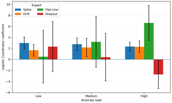
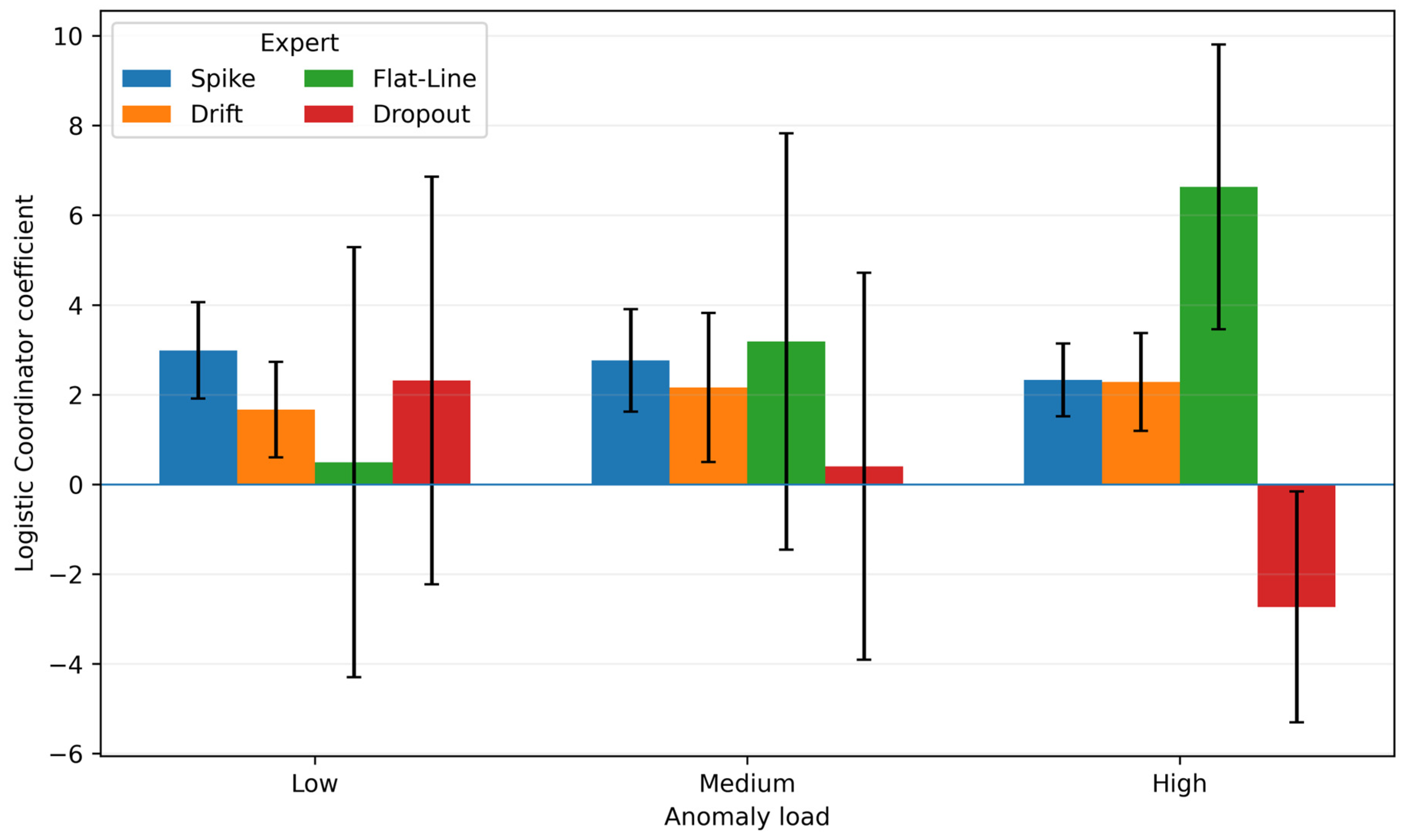
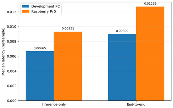
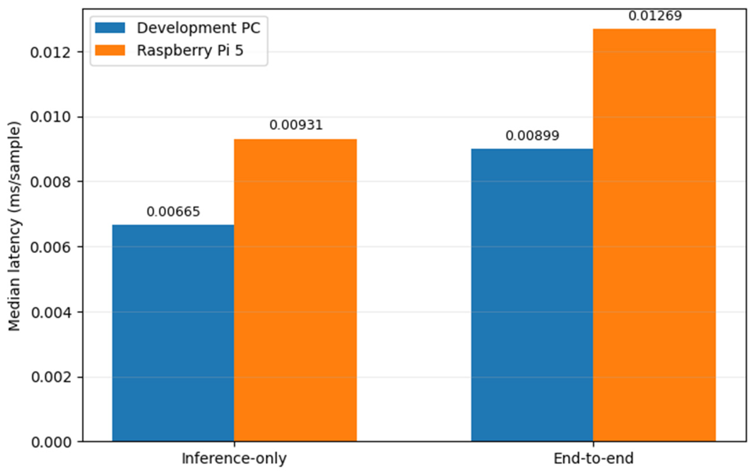

Disclaimer/Publisher’s Note: The statements, opinions and data contained in all publications are solely those of the individual author(s) and contributor(s) and not of MDPI and/or the editor(s). MDPI and/or the editor(s) disclaim responsibility for any injury to people or property resulting from any ideas, methods, instructions or products referred to in the content. |
© 2026 by the authors. Licensee MDPI, Basel, Switzerland. This article is an open access article distributed under the terms and conditions of the Creative Commons Attribution (CC BY) license.