Multi-Time-Scale GAT-Based Online Optimal Regulation Method for Distribution Networks Considering Novel Source-Load Integration

Abstract

The large-scale integration of distributed photovoltaic (PV) generation and electric vehicles (EVs) increases uncertainty in distribution-network source and load conditions and complicates system operation. Conventional optimization methods based on iterative solutions and day-ahead forecasts may not meet the real-time operating requirements of active distribution networks. Therefore, a multi-time-scale Graph Attention Network (GAT)-based online optimization and control method is proposed for distribution networks with emerging source-load resources. First, stochastic and time-varying source-load scenarios are generated using a PV output model and an EV charging-load model. Second, the reactive power optimization model is solved offline to construct a control-decision dataset that accounts for the different dynamic responses of the regulation devices. The GAT is then trained to learn the nonlinear mapping from distribution-network operating states to control decisions, forming a multi-time-scale online decision-making model. The long-time-scale model regulates discrete devices, whereas the short-time-scale model regulates continuous devices. For the IEEE 33-bus case study, the average GAT inference time is 0.0703 s, compared with 83.7667 s for PSO. The hour-level model achieves MAE/RMSE values of 0.0398/0.0407, while the 15 min model achieves 0.0374/0.0397; all bus voltages are maintained within 0.95–1.05 p.u. after optimization. The model is validated under the tested operating distribution; broader robustness and field applicability require further validation.

1. Introduction

As carbon-peaking and carbon-neutrality goals progress, the integration of distributed photovoltaic (PV) generation [1] and electric vehicles (EVs) [2] into distribution networks continues to increase. Although these resources provide additional operational flexibility, their large-scale deployment introduces substantial source-load uncertainty and can increase voltage deviations and network losses [3]. At the same time, coordinating heterogeneous reactive power regulation devices creates opportunities for operational optimization. However, the heterogeneous characteristics and response times of these devices substantially increase the complexity of reactive power optimization. Consequently, distribution-network operation involves a high-dimensional decision space, strong nonlinear coupling, and limited applicability of conventional online optimization methods [4].

Existing approaches to reactive power optimization in distribution networks mainly include mathematical optimization methods [5,6,7,8,9] and heuristic algorithms [10,11]. Mathematical approaches use techniques such as second-order-cone relaxation and linearization to obtain convex formulations for which a global optimum can, in principle, be found. However, large-scale distribution networks can incur high computational costs because of Jacobian-matrix inversion and can be sensitive to initial conditions, limiting adaptability to rapidly changing operating conditions. Heuristic algorithms improve global-search capability through population-based search. As the number of controllable units, including PV systems and reactive power regulation devices, increases, the search space expands exponentially and creates a substantial computational burden. Consequently, iterative solution procedures may not satisfy the time requirements of 15 min or even second-level online regulation.

Recent advances in machine learning have enabled data-driven approaches [12,13,14,15,16,17,18,19] for power-system optimization. By learning from historical dispatch data, these methods establish nonlinear mappings between operating states and control strategies, avoiding iterative optimization during online implementation and increasing decision-making speed. References [12,13,14] use XGBoost (Extreme Gradient Boosting), a Deep Extreme Learning Machine (DELM), and a Convolutional Neural Network (CNN), respectively, to approximate reactive power control strategies. However, these studies use conventional load profiles and therefore do not account for the stochastic, time-varying fluctuations introduced by emerging source-load resources or the reactive power capability of PV inverters as control variables. References [15,16,17,18,19] further use Graph Neural Networks (GNNs) and Reinforcement Learning (RL) to construct multi-time-scale hierarchical optimization models. Their decision inputs still depend heavily on day-ahead or intraday forecasts [20,21], and accumulated forecast errors can cause online control outputs to lag behind actual operating conditions, limiting the response to short-term source-load fluctuations.

Therefore, a multi-time-scale Graph Attention Network (GAT)-based online optimization and control method is proposed for distribution networks with emerging source-load resources. During the offline stage, PV-generation and EV charging-load models generate stochastic, time-varying source-load scenarios. A reactive power optimization model is then formulated while accounting for the distinct dynamic responses of the regulation devices. Solving this model offline produces a control-decision dataset covering a wide range of operating conditions. The GAT is subsequently trained to capture the nonlinear relationship between distribution-network operating states and the corresponding control decisions, thereby establishing a multi-time-scale online decision-making framework. During online operation, real-time measurements are provided to the trained GAT, which rapidly generates control decisions through forward inference according to device response characteristics. Results for the IEEE 33-bus test system demonstrate accurate online inference and computational feasibility, while broader real-time and field applicability remain to be validated.

Electric-vehicle charging is a time-varying and spatially distributed load rather than a fixed demand profile. Its coincidence or mismatch with PV generation can amplify net-load fluctuations, increase the risk of midday overvoltage and evening undervoltage, and make the coordination of discrete and continuous reactive power devices more difficult. The contributions of this study are the construction of source-load scenarios that include EV charging variability, the coordination of long- and short-time-scale reactive power devices, and the GAT-based online approximation of feasible control decisions.

2. Modeling of Distributed Photovoltaic Generation and Electric-Vehicle Loads

2.1. PV Output Model Based on Measured Meteorological Data

The active power output of distributed photovoltaic (PV) systems is primarily determined by solar irradiance (L) and ambient temperature (T). To represent the time-varying behavior of PV generation under realistic operating conditions, measured meteorological data are incorporated into the model, and the resulting power output is calculated according to the operating characteristics of PV generation [22].

Under steady-state conditions, the photovoltaic output power is given by Equation (1):

$$P_{\mathrm{PV}}=P_{\mathrm{PV},\mathrm{N}}{\displaystyle \frac{L}{L_{\mathrm{N}}}}\left[1+{\alpha }_{\mathrm{PV}}\left(T_{\mathrm{PV}}-T_{\mathrm{PV},\mathrm{N}}\right)\right]$$

(1)

where P_PV,N is the rated output power; L is the actual light intensity; L_N is the standard irradiation intensity (1000 W/m²); T denotes the ambient temperature; T_N represents the standard test temperature; and α_PV denotes the power temperature coefficient.

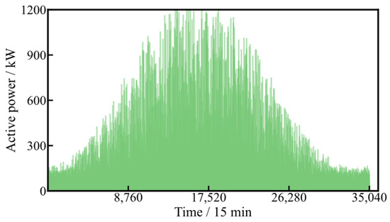
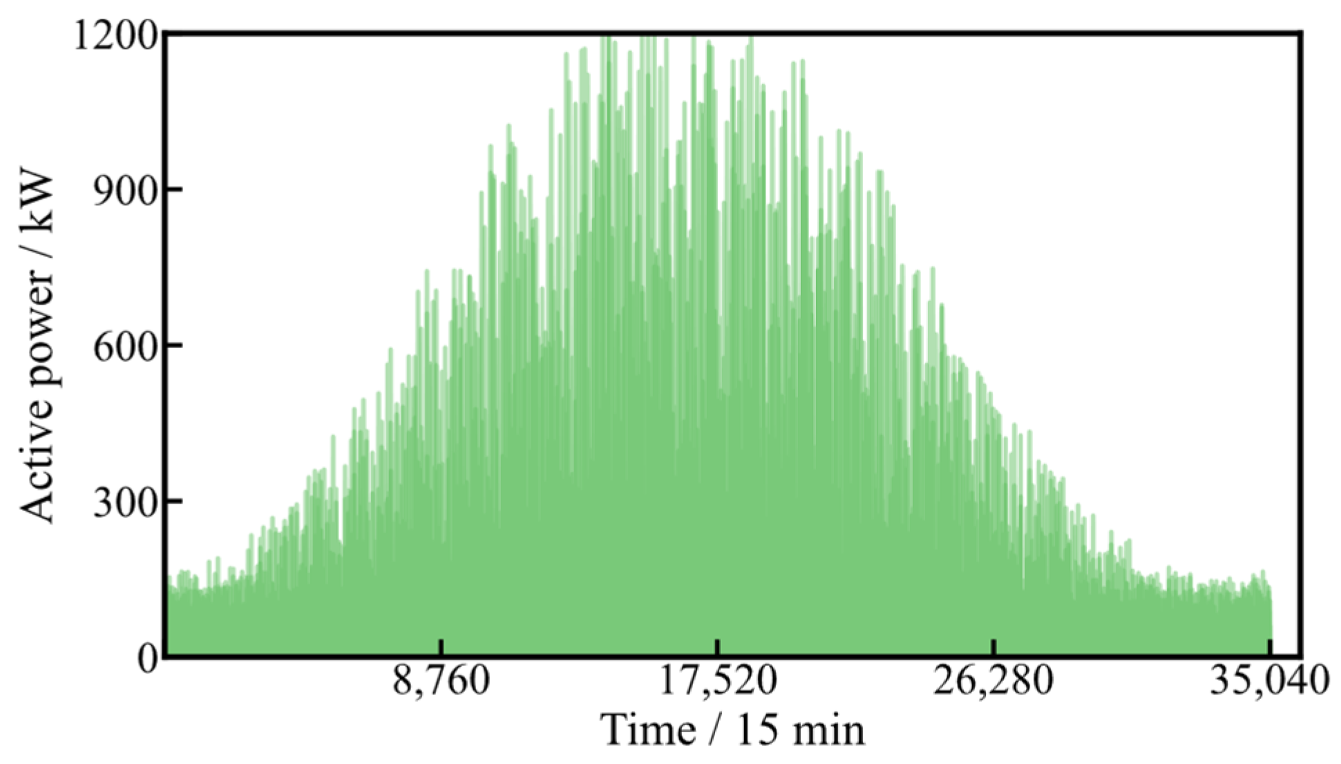
Using 15 min time-series data for solar irradiance L and ambient temperature T from the Meteonorm 7.3 meteorological database, the PV output is calculated using Equation (1). The resulting PV power time series is shown in Figure 1. The meteorological location is set to Shijiazhuang, Hebei, China (38.04 N, 114.51 E), and the sequence represents one typical meteorological year with 35,040 samples.

Figure 1. PV power time-series profile for Shijiazhuang, Hebei, China.

2.2. Stochastic EV Load Model Based on the Monte Carlo Method

EV charging demand is influenced by travel patterns, initial battery state of charge, and user charging preferences, resulting in substantial stochastic and temporal variability. To quantify the effect of EV penetration on distribution-network load profiles, we developed an aggregated EV charging-load model based on the statistical properties of user charging behavior. Probability distributions are specified for the initial state of charge (SOC) and charging start time of each vehicle category, and the charging demand of each EV is calculated from its battery capacity and charging power. By aggregating individual charging profiles, the regional EV charging load curve can be derived.

The EV charging start time is modeled as a normally distributed variable [23], whose probability density function is given by Equation (2):

$$f_T(t)={\displaystyle \frac{1}{\sqrt{2\pi }{\sigma }_T}}\exp [-{\displaystyle \frac{{(t-{\mu }_T)}^2}{2{\sigma }_T^2}}]$$

(2)

where μ_T is the mean charging start time and σ_T is the standard deviation.

Once charging begins, each EV is assumed to charge at constant power; its charging duration is given by Equation (3):

$$T_f={\displaystyle \frac{(1-S_{\mathrm{OC}})\times C}{P_{\mathrm{EV}}}}$$

(3)

where C is the battery capacity; S_OC is the initial state of charge, and P_EV corresponds to the charging power.

To capture the stochasticity of charging behavior across an EV fleet, the Monte Carlo method is used to generate charging-demand scenarios. For a system of m EVs, the charging parameters of each vehicle are sampled from the probability density functions of the initial SOC and charging start time, as given by Equation (4).

$$\begin{array}{l}{t}_{0,i} ~ f_T\left(x\right),\\ S_{\mathrm{OC}i} ~ f_{SOC}\left(x\right), i=1,2,\dots ,m\end{array}$$

(4)

where f_SOC(•), f_T(•) denote the probability distribution functions for S_OC and charging start time, respectively, and m represents the total vehicle count.

Using the sampled S_OC and charging start time, Equation (3) determines the charging duration and charging state of each EV on the discrete time-scale. Superimposing the charging power of all vehicles yields the aggregated EV load at time t, calculated using Equation (5):

$$L_t={\displaystyle \sum _{i=1}^N}{P}_{i,t}$$

(5)

where P_i,t denotes the charging power of the i-th EV at time step t.

3. Methodology: Multi-Time-Scale GAT-Based Online Decision-Making

This section presents the methodology of the proposed multi-time-scale GAT-based online optimization method. The procedure comprises four stages: formulation of the reactive power optimization problem and its operating constraints; generation of Particle Swarm Optimization (PSO)-derived control-decision labels at two time scales; continuous encoding and decoding of discrete device states; and supervised GAT training followed by coordinated hour-level and 15 min online inference. The hour-level model determines the baseline settings of discrete and continuous devices, whereas the 15 min model updates fast-response continuous resources using the latest operating measurements.

The methodological contribution lies in the coordination of three elements: state representation driven by real-time measurements, time-scale-aware updates of heterogeneous devices, and graph-attention learning of the operating-state-to-control-decision mapping. PSO is used offline to generate feasible control-decision labels, whereas GAT performs the online forward inference; thus, the framework is a coordinated surrogate-based optimization method rather than a simple aggregation of independent algorithms.

3.1. Reactive Power Optimization Problem Formulation

(1)

Objective function

To improve both operational economy and voltage quality, we formulate a reactive power optimization model that minimizes system active power loss and average nodal voltage deviation. The objective function is given by Equation (6):

$$\min F=P_{\mathrm{loss}}\left(Q_{\mathrm{PV}},Q_{\mathrm{SVC}},y_{\mathrm{SCB}},y_{\mathrm{OLTC}}\right)+\lambda {\displaystyle \frac{1}{N}}{\displaystyle \sum _{i=1}^N}\left|{\displaystyle \frac{U_i-U_{\mathrm{N}}}{U_{\mathrm{N}}}}\right|$$

(6)

where N denotes the number of buses; U_i denotes the voltage magnitude at bus i; U_N is the rated voltage, and λ is the penalty coefficient for voltage deviation; and the relevant control variables include PV reactive power output Q_PV, static var compensator (SVC) reactive power output Q_SVC, shunt capacitor bank (SCB) switching group number y_SCB and on-load tap-changing transformer (OLTC) gear y_OLTC. This formulation provides the mathematical basis for the subsequent time-scale-specific control decisions.

(2)

Constraints

(1) The allowable range for the reactive power output of the PV system is given by Equation (7):

$$Q_{\mathrm{PV}}=\pm \sqrt{{\left(1.1S_{\mathrm{N}}\right)}^2-P_{\mathrm{PV}}^2}$$

(7)

where S_N represents the rated power of the photovoltaic source.

(2) The power flow constraints of the distribution network are given by Equation (8):

$$\left\{\begin{array}{l}{P}_i-V_i{\displaystyle \sum _{j=1}^N}{V}_j(G_{ij}\cos {\theta }_{ij}+B_{ij}\sin {\theta }_{ij})=0\\ Q_i-V_i{\displaystyle \sum _{j=1}^N}{V}_j(G_{ij}\sin {\theta }_{ij}-B_{ij}\cos {\theta }_{ij})=0\end{array}\right.$$

(8)

where P_i and Q_i denote the injected active and reactive power, respectively; V_i and V_j denote the bus voltage magnitudes; G_ij and B_ij are the conductance and susceptance elements of the bus-admittance matrix; θ_ij denotes the phase angle difference between buses.

(3) System security constraints are given by Equation (9):

$$\left\{\begin{array}{c}{U}_{\min }\le U_i\le U_{\max }\\ \left|{\theta }_i-{\theta }_j\right|\le {\left|{\theta }_i-{\theta }_j\right|}_{\max }\end{array}\right.$$

(9)

where U_min and U_max denote the minimum and maximum bus voltage magnitudes, respectively; |θ_i−θ_j|_max is the maximum phase angle difference.

(4) Control variable limits are given by Equation (10):

$$\left\{\begin{array}{l}{Q}_{\mathrm{PVmin}}\le Q_{\mathrm{PV}}\le Q_{\mathrm{PVmax}}\\ Q_{\mathrm{SVCmin}}\le Q_{\mathrm{SVC}}\le Q_{\mathrm{SVCmax}}\\ y_{\mathrm{SCBmin}}\le y_{\mathrm{SCB}}\le y_{\mathrm{SCBmax}}\\ T_{\min }\le y_{\mathrm{OLTC}}\le T_{\max }\end{array}\right.$$

(10)

where Q_PVmax and Q_PVmin represent the maximum and minimum reactive power compensation capacities of the PV units, respectively; Q_SVCmax and Q_SVCmin denote the capacity bounds of the static var compensator, respectively; y_SCBmax and y_SCBmin stand for the upper and lower limits on the number of shunt capacitor switching groups, respectively; T_max and T_min correspond to the upper and lower tap positions of the OLTC, respectively.

Reactive power regulation devices differ substantially in response speed and permissible operating frequency. PV inverters and SVCs provide fast, continuous regulation, whereas SCBs and OLTCs operate in discrete steps and should not be switched frequently. Accordingly, control decisions are divided into two time scales: the long-time-scale layer sets the operating states of discrete devices, while the short-time-scale layer updates continuous reactive power outputs on a rolling basis. This hierarchy balances regulation performance with switching frequency and device lifetime.

3.2. Multi-Time-Scale Reactive Power Optimization Based on PSO

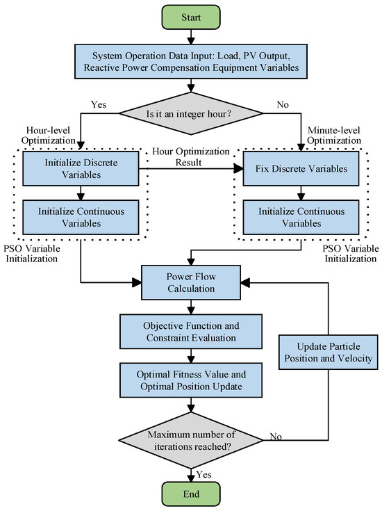
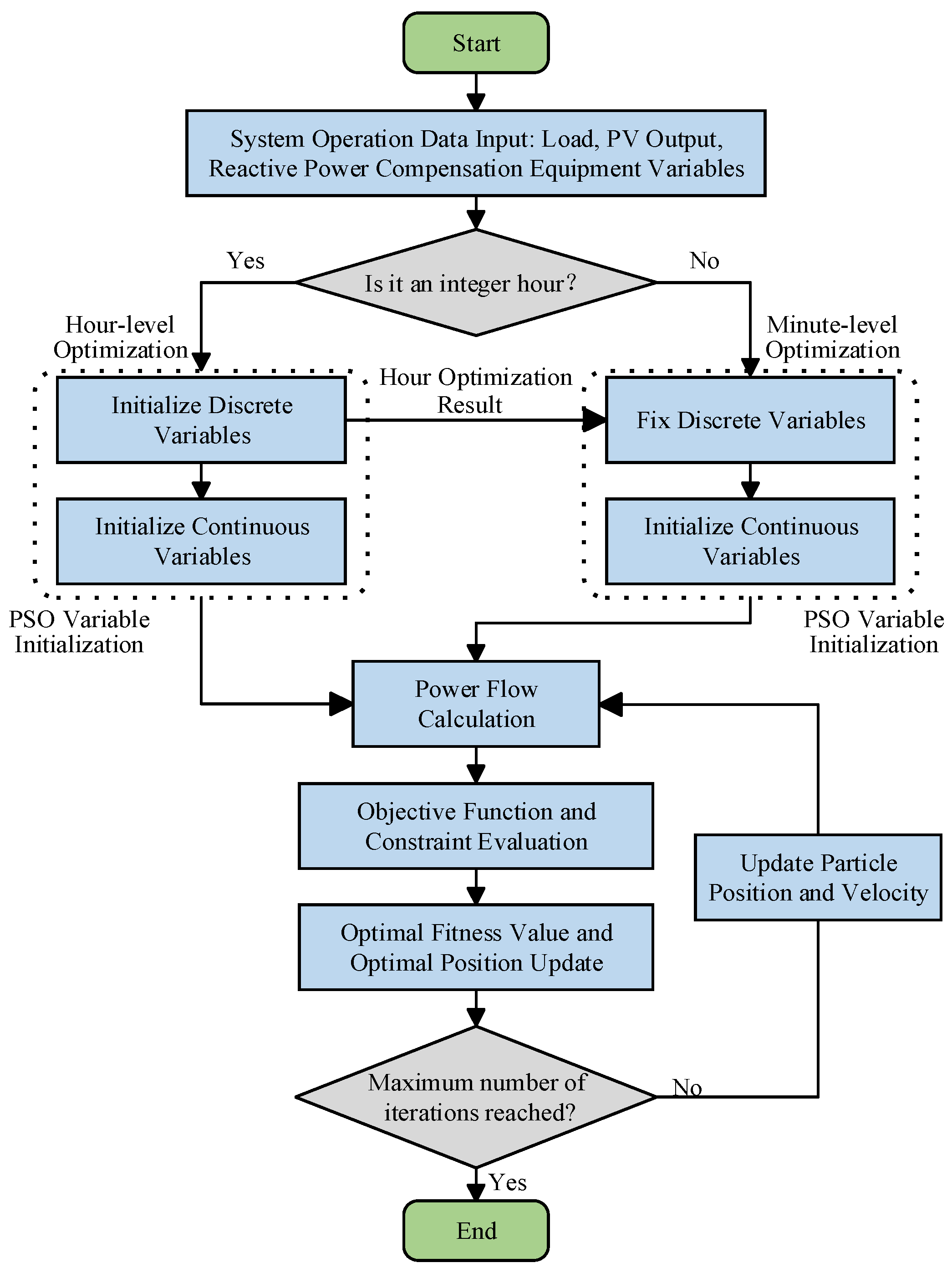
To enable multi-time-scale scheduling of reactive power regulation devices, we introduce a time-scale-dependent variable-update strategy within a unified PSO framework. The workflow of the proposed PSO-based reactive power optimization method is shown in Figure 2. The offline stage generates the operating-state and control-decision pairs used for subsequent GAT training. At the long time-scale, this optimization uses the common objective and constraint set defined in Section 3.1, namely, Equations (6)–(10).

Figure 2. PSO-based reactive power optimization workflow.

The procedure uses annual sequential load profiles and distributed-generation outputs as inputs. The operating horizon is partitioned chronologically, and each operating state is optimized using a rolling scheme. Different update rules are used for long- and short-time-scale devices. The procedure is as follows.

(1)

Operating data input: The inputs comprise load demand, PV generation output, and the parameters of the reactive power regulation devices.

(2)

Time-scale identification: The control layer is selected according to the current optimization instant. Long-time-scale optimization is executed at the beginning of each hour, whereas short-time-scale optimization is performed at 15 min intervals within the hour.

(3)

Optimization variable initialization: At the hour level, both discrete and continuous control variables are initialized according to the operating characteristics of long-time-scale devices. The discrete variables are the OLTC tap position and SCB switching state, whereas the continuous variables are the reactive power outputs of PV units and SVCs. During the 15 min optimization stage, the discrete variables remain fixed at their hour-level values, and only continuous variables such as PV reactive power and SVC reactive power output are initialized and iteratively adjusted to avoid excessive switching of discrete devices.

(4)

Power flow analysis and state assessment: For each particle, the associated reactive power control variables are passed to the distribution network power-flow solver. The resulting operating variables are used to evaluate the defined objectives and constraints and to compute the particle fitness.

(5)

Particle update: The personal-best and global-best solutions are updated according to particle fitness, and particle velocities and positions are then updated using the PSO rules.

(6)

Termination criterion: If the maximum number of iterations has not been reached, the algorithm returns to Step (4); otherwise, it outputs the best found reactive power control decision for the current operating condition.

This multi-time-scale strategy reflects the operating characteristics of long- and short-time-scale devices and prevents unnecessary switching of discrete devices under short-term fluctuations. However, PSO requires iterative optimization for each operating snapshot, which limits online decision-making speed. The resulting two-level dispatch scheme sets an hourly control baseline and applies 15 min rolling corrections, providing the basis for the GAT-based online decision-making model.

3.3. State Encoding of Reactive Power Devices

The regulation devices involve continuous and discrete control variables. In a data-driven reactive power optimization model, directly learning discrete variables can produce discontinuous outputs and infeasible control decisions. To address this issue, we used a continuous encoding method based on Roulette Wheel Selection [24] to map discrete states to normalized continuous scalar codes. Taking an on-load voltage-regulating transformer with m regulating gears as an example, the continuous code corresponding to the i-th gear is defined by Equation (11):

$$y_{\mathrm{e}}={\displaystyle \frac{2i-1}{2m}}$$

(11)

where y_e is the encoding value corresponding to the i-th tap position.

The discrete control gear y_d is recovered by decoding the continuous code y_e using Equation (12):

$$y_{\mathrm{d}}=\left\{\begin{array}{l}1,0\le y_{\mathrm{e}}\le {\displaystyle \frac{i}{m}}\\ i,{\displaystyle \frac{i-1}{m}}<y_{\mathrm{e}}\le {\displaystyle \frac{i}{m}}\end{array}\right.$$

(12)

This encoding converts discrete device states into learnable continuous variables, allowing the GAT to learn all control strategies in a unified output space. This encoding provides continuous regression targets for GAT training and supports gradient-based optimization of the network outputs. The decoded outputs are then converted into feasible discrete device states.

For a device with m discrete states, Equation (11) maps the i-th state to a normalized scalar code in the unit interval, with distinct states assigned distinct code positions. Equation (12) decodes the predicted scalar by identifying the corresponding ordered interval and returns one feasible discrete state. The code is therefore a normalized roulette-wheel-style representation rather than a probability vector. During training, the continuous code is used as the regression target, which allows gradient-based optimization of the GAT output; during inference, interval decoding is applied after the forward pass as deterministic post-processing, and the discrete decoding operation itself is not claimed to be differentiable.

3.4. GAT-Based Reactive Power Optimization

Nodal voltages and power flows in a distribution network are coupled through line impedances. Accordingly, the network is represented as a graph G(V,E), where V is the set of buses and E is the set of branches. Under the supervised learning framework, the initial node-feature vector h_i for bus i is formed from measured variables in the current operating snapshot, including distributed PV active power and load power. The output labels comprise the reactive power outputs of PV inverters and SVCs, the number of SCB groups in service, and OLTC tap positions. This graph representation provides the structural input for learning the mapping from operating states to control decisions.

A conventional Graph Convolutional Network (GCN) uses fixed adjacency weights, making it difficult to distinguish coupling strengths between buses. To address this limitation, we introduce a GAT, which learns node coupling adaptively through an attention mechanism and captures the nonlinear mapping from distribution network operating states to control decisions.

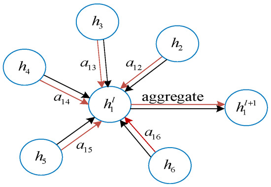
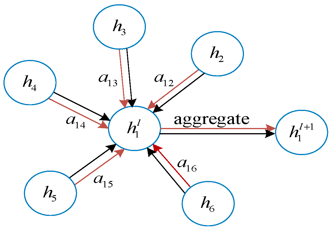
The core component of GAT is the Graph Attention Layer (GAL), shown in Figure 3.

Figure 3. Structure of the Graph Attention Layer.

For node i and its neighbor j, the attention coefficient is first calculated and normalized as given by Equations (13) and (14):

$$e_{ij}={\overrightarrow{a}}^T(W{\overrightarrow{h}}_i\parallel W{\overrightarrow{h}}_j)$$

(13)

$$a_{ij}=\mathrm{soft}\max (e_{ij})={\displaystyle \frac{\exp (\mathrm{LeakyReLU}({\overrightarrow{a}}^T[W{\overrightarrow{h}}_i\parallel W{\overrightarrow{h}}_j]))}{{\displaystyle \sum _{k\in N\left(i\right)}}\exp (\mathrm{LeakyReLU}({\overrightarrow{a}}^T[W{\overrightarrow{h}}_i\parallel W{\overrightarrow{h}}_k]))}}$$

(14)

where ${\overrightarrow{h}}_i$, ${\overrightarrow{h}}_j$ denote the node feature vectors; W is a shared weight matrix; ‖ denotes feature concatenation; ${\overrightarrow{a}}^T$ denotes the attention mapping function; N(i) denotes the set of neighboring buses of bus i, including the bus itself, and leaky ReLU represents the activation function.

The node features are then updated using the normalized attention weights, as given by Equation (15):

$$h_i^{(l+1)}=\sigma (\sum _{j\in N\left(i\right)}{a}_{ij}\cdot W\cdot h_j)$$

(15)

To improve the model’s ability to represent complex source-load conditions, we incorporate multi-head attention. Independent attention heads learn structural correlations in different feature subspaces, such as voltage rises caused by PV injection and voltage drops under heavy loading. The resulting features are fused to improve mapping stability, as given by Equations (16) and (17):

$$h_i^{(l+1)}={\Vert }_{k=1}^K\sigma \left(\sum _{j\in N\left(i\right)}{a}_{ij}^k{W}^k{h}_j\right)$$

(16)

$$h_i^{(l+1)}=\sigma \left({\displaystyle \frac{1}{K}}{\displaystyle \sum _{k=1}^K\sum _{j\in N\left(i\right)}{a}_{ij}^k{W}^k{h}_j}\right)$$

(17)

where K denotes the number of attention heads; ‖ denotes feature concatenation; $a_{ij}^k$ and $W^k$ represent the weight coefficients and weight parameters of the k-th attention mechanism, respectively. The architecture and training configuration of the network are summarized in Table 1.

Table 1. Architecture and hyperparameters of the GAT model.

Layer	Structure	Parameters	Activation Function	Output Size
Layer 1	Input Layer	--	--	X: 33 × F, A: 33 × 33
Layer 2	GATConv Layer	4 attention heads, dropout = 0.2	GeLU	33 × 64
Layer 3	GATConv Layer	4 attention heads, dropout = 0.2	GeLU	33 × 64
Layer 4	Flatten Layer	--	--	1 × 2112
Layer 5	Dense Layer	1024 neurons	GeLU	1 × 1024
Layer 6	Dense Layer	512 neurons	GeLU	1 × 512
Layer 7	Output Layer 1	7 neurons	Linear	1 × 7
Layer 8	Output Layer 2	3 neurons	Linear	1 × 3 (hour-level only)
Training	Optimizer	Adam	--	--
	Learning rate	1 × 10−3	--	--
	Batch size	64	--	--
	Max. epochs	300	--	--
	Early stopping	patience 30	--	--
	Loss function	MSE on normalized outputs	--	--

3.5. Multi-Time-Scale GAT-Based Online Decision-Making Model

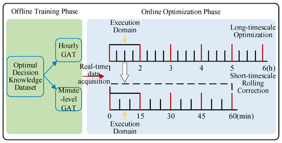
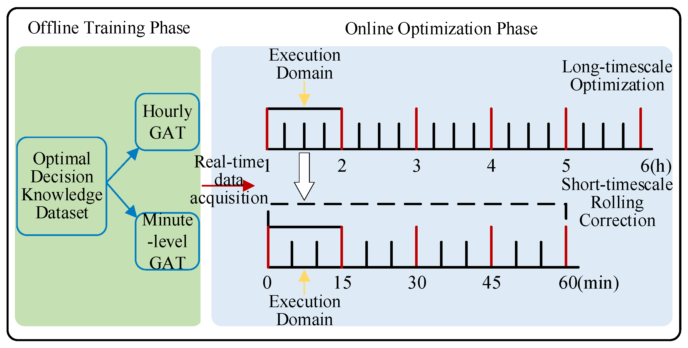
To address the high computational cost of PSO and prevent forecast errors from causing unnecessary discrete-device switching, we constructed a multi-time-scale GAT-based online decision-making model. The model uses real-time measurements rather than day-ahead or hourly forecasts. Short-term fluctuations are handled by rolling optimization at the short-time-scale, and the coordination between decision levels is shown in Figure 4. This stage connects the offline labels and trained GAT models to the online control workflow.

Figure 4. Schematic Diagram of the Proposed Multi-Time-Scale GAT-Based Online Decision-Making Framework.

(1)

Hour-Level Decision-Making Stage:

The hour-level GAT model provides the baseline decision at the long-time-scale. At the beginning of each hour, it receives the current distribution network operating state and outputs continuous and discrete control decisions. Because discrete devices have slower response times and should not be switched frequently, their states are held constant during the following hour. The continuous outputs initialize the 15 min rolling correction. Specifically, the hour-level decision variables include the continuous reactive power outputs of PV inverters and SVCs, together with the discrete switching states of SCBs and the tap position of the OLTC. These variables are optimized according to Equation (6) and subject to the constraints in Equations (7)–(10). The resulting discrete states remain fixed over the following four 15 min intervals, while the continuous decisions initialize the 15 min rolling correction.

(2)

15-Min Rolling-Correction Stage:

The 15 min GAT model performs short-time-scale rolling correction. At each update, the latest operating state is collected, the hour-level discrete decisions are held fixed, and only continuous reactive power resources are updated.

The coordinated long- and short-time-scale GAT decision model is given by Equations (18) and (19):

$$\left[Q_{\mathrm{PV}}^h,Q_{\mathrm{SVC}}^h,y_{\mathrm{SCB}}^h,y_{\mathrm{OLT}C}^h\right]=f_{GAT}^{\mathrm{h}}\left(P_{\mathrm{L}}^h,Q_{\mathrm{L}}^h,P_{\mathrm{PV}}^h,Y\right)$$

(18)

$$\left[\begin{array}{c}{Q}_{\mathrm{PV}}^t,Q_{\mathrm{SVC}}^t\end{array}\right]=f_{GAT}^t\left(P_{\mathrm{L}}^t,Q_{\mathrm{L}}^t,P_{\mathrm{PV}}^t,y_{\mathrm{SCB}}^{\mathrm{h}},y_{\mathrm{OLTC}}^h,Y\right)$$

(19)

where $Q_{\mathrm{PV}}^h$, $Q_{\mathrm{SVC}}^h$, $y_{\mathrm{SCB}}^h$, $y_{\mathrm{OLTC}}^h$ represent the PSO-derived PV reactive power output, PSO-derived SVC compensation capacity, PSO-derived shunt capacitor switching group number, and PSO-derived OLTC gear coding value derived from the hour-level model, respectively; $P_{\mathrm{L}}^h$, $Q_{\mathrm{L}}^h$ and $P_{\mathrm{PV}}^h$ correspond to the hour-level active load, reactive load, and PV active power output, respectively; $Q_{\mathrm{PV}}^t$ and $Q_{\mathrm{SVC}}^t$ denote the PSO-derived PV reactive power output and PSO-derived SVC compensation capacity produced by the 15 min model, respectively; $P_{\mathrm{L}}^t$, $Q_{\mathrm{L}}^t$ and $P_{\mathrm{PV}}^t$ signify the 15 min load and PV active output, respectively; Y represents the admittance matrix; and $f_{GAT}$ stands for the mapping function that relates the distribution network operating conditions to the PSO-derived reactive power decisions of the compensation equipment.

Under this coordinated framework, the hour-level model sets stable reference values for discrete devices, whereas the 15 min model continuously adjusts fast-response reactive power resources. This arrangement avoids frequent switching of discrete devices and accommodates short-term source-load fluctuations, enabling data-driven multi-time-scale online reactive power control.

4. Case Study

4.1. Case-Study Configuration

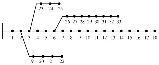
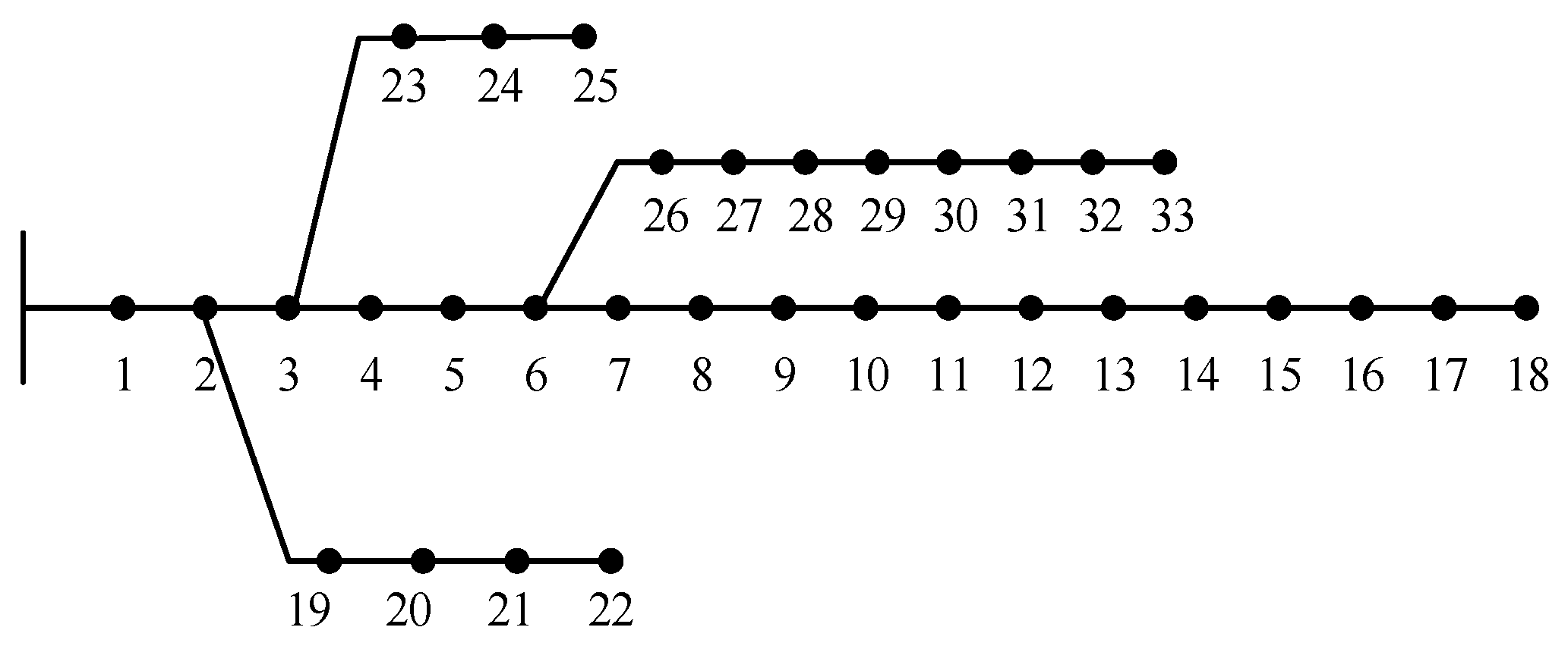
To evaluate the proposed multi-time-scale online optimization model based on the GAT, we conduct simulations on the IEEE 33-bus test system. The case study includes distributed generation (DG) and EV loads, and the resulting network topology is shown in Figure 5. The bus-number labels in Figure 5 have been corrected according to the standard IEEE 33-bus feeder topology, with bus 18 located at the terminal of the main feeder.

Figure 5. IEEE 33-bus model.

(1)

Distributed Resources and Adjustable-Device Allocation

PV units are connected at buses 5, 11, 18, 27, and 33, with capacities of 2 MW, 1 MW, 1 MW, 2 MW, and 1.5 MW, respectively. The maximum PV output is set to 1.1 times the rated capacity to account for short-term overload capability. EV charging loads are connected at buses 9, 16, and 33, with penetration ratios of 20%, 10%, and 10% of the original loads, respectively. The OLTC voltage range is 0.95–1.05 p.u., with a 1% tap step and 11 tap states (−5 to +5). SVCs are installed at buses 14 and 30, each with a capacity of 1000 kvar. SCBs are installed at buses 19 and 23, with 10 groups at each bus and a capacity of 100 kvar per group.

(2)

Time-Series Generation and Load Data

The simulation uses the distribution network’s monitoring interval of 15 min, yielding 35,040 time steps for one year. Base load profiles are generated from the rated IEEE 33-bus loads using typical daily profiles, seasonal factors, and a 5% Gaussian disturbance. EV charging loads are generated with the Monte Carlo model and added to the corresponding buses according to the specified penetration ratios. PV outputs are generated from measured meteorological data and scaled by the installed capacity at each bus. The resulting node-level load is calculated using Equation (20).

$$P_{\mathrm{load},i}=P_{\mathrm{base},i}+P_{\mathrm{EV},i}$$

(20)

where P_base,i and P_EV,i correspond to the base load at node i and the charging load of EVs, respectively.

(3)

Construction of the Control-Decision Dataset

PSO is executed for the generated operating conditions to obtain reactive power control decisions. The resulting operating-state and decision pairs are organized into a dataset. Before model training, the annual dataset is shuffled using a random seed and then divided into training and test sets at a ratio of 9:1. This sample-level random split is adopted because the proposed GAT learns a static mapping from each operating snapshot to its corresponding control decision, rather than a temporal forecasting model. Each sample is constructed from the operating state of a single 15 min interval, and historical or future samples are not used as model inputs; therefore, test labels or future temporal information are not directly used during training.

To generate the control-decision labels, PSO is configured with a population size of 50 particles and a maximum of 100 iterations; the inertia weight decreases linearly from 0.9 to 0.4, and the acceleration coefficients are set to $c_1$ = $c_2$ = 2.0. The search terminates when the change in the global-best fitness falls below 1 × 10⁻⁶ or the maximum number of iterations is reached. Each operating condition is solved with 10 independent runs initialized from different random seeds, and the best-found solution is retained.

(4)

Computational Environment

Model training and testing are performed on Windows using VS Code. Power flow calculations use the MATPOWER toolbox (version 7.1). The hardware comprises an AMD Ryzen 7 6800H processor operating at 3.20 GHz and 16 GB RAM.

4.2. Evaluation of Control-Decision Prediction Performance

To evaluate how well the GAT learns the mapping from operating conditions to control decisions, we used DELM [13] and GCN [15] as benchmark models. Performance is assessed using the reported error metrics. For a fair comparison, the network architectures and key hyperparameters of all models are optimized using Bayesian optimization [25]. The resulting GAT architecture and hyperparameter configuration are summarized in Table 1.

Table 1 summarizes the architecture and hyperparameters shared by the hour-level and 15 min GAT models. Although their architectures are identical, the models are trained independently. The hour-level model uses F = 3 input features and produces continuous and discrete outputs, whereas the 15 min model uses F = 5 input features and outputs only continuous variables.

After the architecture and key hyperparameters have been selected, the control-decision prediction performance of each model is summarized in Table 2.

Table 2. Comparison of control-decision prediction performance.

Model	Hour-Level Model MAE	Hour-Level Model RMSE	Hour-Level Model MDCE	15 Min Model MAE	15 Min Model RMSE	Average Computation Time (s)
PSO	--	--	--	--	--	83.7667
GAT	0.0398	0.0407	0.0412	0.0374	0.0397	0.0703
GCN	0.0588	0.0678	0.0638	0.0518	0.0624	0.0608
DELM	0.0705	0.0984	0.0943	0.0625	0.0847	0.0361

Mean absolute error (MAE) and root mean square error (RMSE) are used to evaluate each model on the corresponding test set. The RMSE is more sensitive to large errors and therefore emphasizes extreme deviations. Because the hour-level model outputs both continuous and discrete variables, the mean discrete control error (MDCE) is used to assess the discrete settings recovered from the continuous codes. It is defined by Equation (21):

$$M_{\mathrm{DCE}}={\displaystyle \frac{1}{N}}{\displaystyle \sum _{i=1}^N}|{\widehat{t}}_i-t_i|$$

(21)

where $t_i$ and ${\widehat{t}}_i$ are the true and predicted decoded gear settings of the discrete device, respectively, and N represents the sample size.

The GAT outperforms both the GCN and DELM at both time scales. At the hour level, the GAT achieves an MAE/RMSE of 0.0398/0.0407, corresponding to reductions of approximately 32.3%/40.0% and 43.6%/58.6% relative to the GCN and DELM, respectively. Its MDCE is 0.0412, which is also lower than those of the benchmark models. At the 15 min level, the GAT achieves an MAE/RMSE of 0.0374/0.0397. These results indicate that the attention mechanism captures non-uniform electrical coupling between buses and improves the learning of control decisions.

The GAT requires slightly more inference time than DELM because it computes attention weights, but it is substantially faster than iterative PSO. In the IEEE 33-bus simulation, the GAT therefore provides fast online inference while maintaining high prediction accuracy.

4.3. Evaluation of Reactive Power Optimization Performance

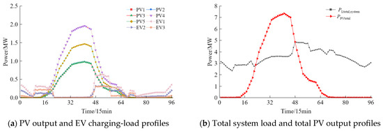
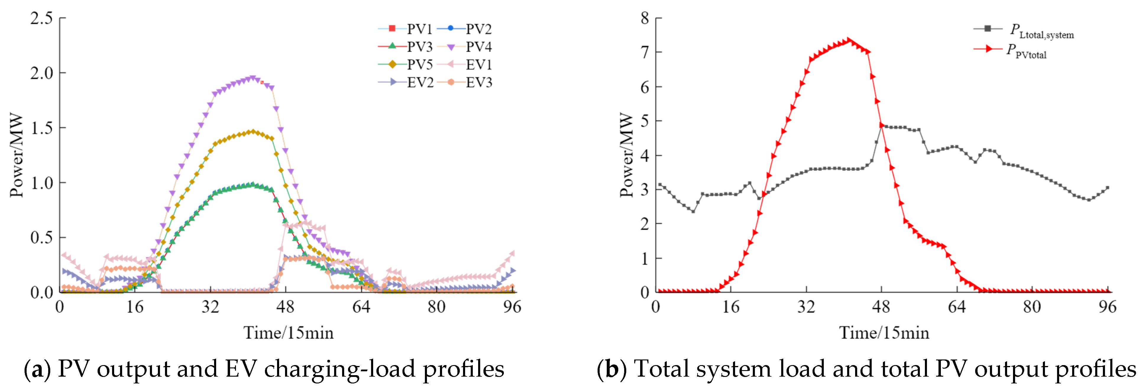
To further evaluate the proposed multi-time-scale rolling GAT model, we analyzed a typical summer day. Reactive power optimization results are examined over 96 intervals at 15 min resolution, and the total system load and PV generation profiles are shown in Figure 6.

Figure 6. Source-load fluctuation profiles.

As shown in Figure 6a, PV generation is concentrated around midday, whereas EV charging demand is distributed across multiple periods and partially overlaps with the PV profile. As shown in Figure 6b, the total system load remains relatively stable because EV charging is distributed over time. In contrast, total PV output peaks at midday and falls rapidly to zero in the evening, producing substantial net-load fluctuations. This temporal mismatch creates simultaneous risks of midday overvoltage and evening undervoltage and increases the complexity of reactive power regulation.

4.3.1. Analysis of the Optimization Objectives

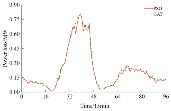
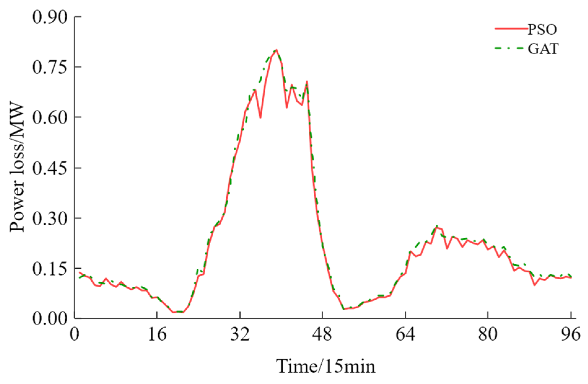
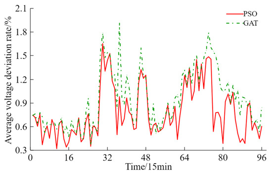
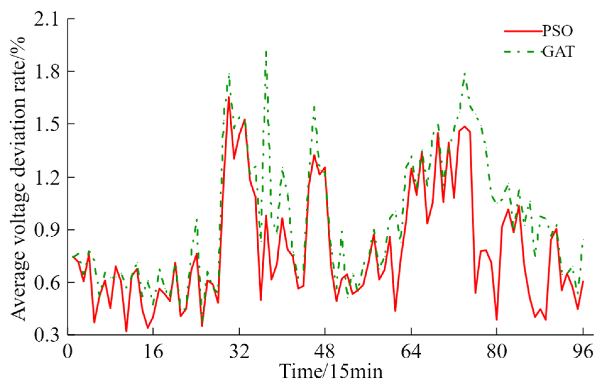
We compare the PSO and GAT models using system active power loss and average nodal voltage deviation, the two optimization objectives. The results are shown in Figure 7 and Figure 8.

Figure 7. Comparison of system active power loss.

Figure 8. Comparison of average system voltage deviation.

The average voltage deviation measures the overall deviation of bus voltages from the rated value. It is defined by Equation (22):

$$\Delta U_{\mathrm{average}}={\displaystyle \frac{1}{N}}{\displaystyle \sum _{i=1}^N}\left|{\displaystyle \frac{U_i-U_{\mathrm{N}}}{U_{\mathrm{N}}}}\right|\times 100\%$$

(22)

Across the 96 intervals, the two methods exhibit closely aligned control trends. The GAT’s active-power-loss curve closely follows the PSO curve, with only small deviations during the high-PV-output period at midday. The GAT’s average voltage deviation is slightly higher than the PSO value; the difference increases during periods of stronger fluctuation but remains limited.

To quantify the overall performance of both methods under identical operating conditions, we calculated the corresponding statistics over the evaluation periods; the results are summarized in Table 3.

Table 3. Comparison of reactive power optimization results for PSO and GAT.

Model	Average Voltage Deviation ∆Uaverage%	Average Network Loss (MW)	Average Objective Value
PSO	0.7839	0.2239	0.0526
GAT	0.9512	0.2331	0.0561

PSO yields lower values for all reported optimization metrics because it directly solves the optimization problem for each operating condition. The GAT approximates the PSO-derived decisions without online iterative optimization. The GAT’s average voltage deviation and network loss are 0.9512% and 0.2331 MW, respectively, compared with 0.7839% and 0.2239 MW for the PSO. These results show that the GAT reproduces the PSO-derived control behavior while substantially reducing online computation time.

4.3.2. Voltage-Regulation Performance at Source-Load Connection Buses

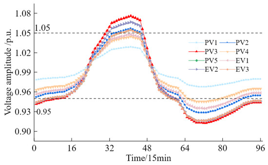
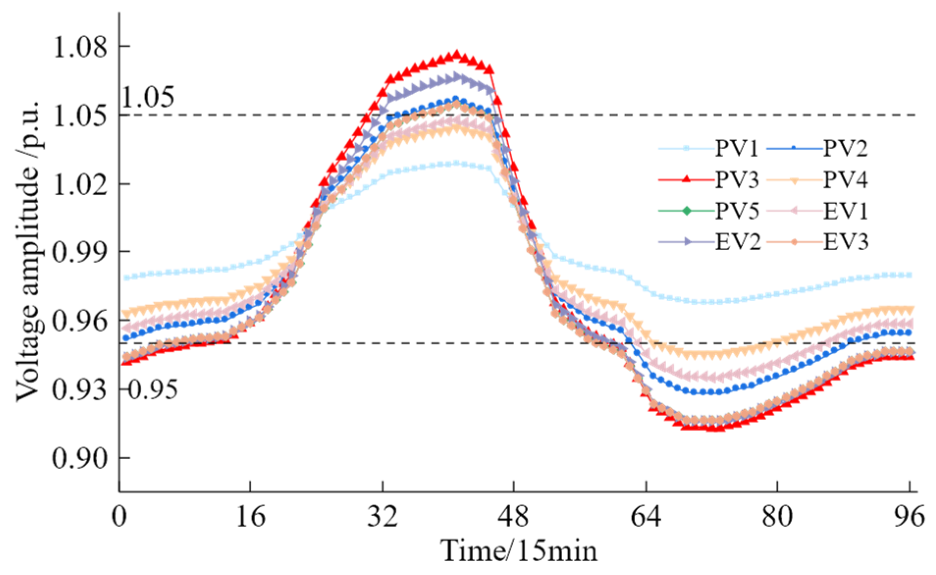
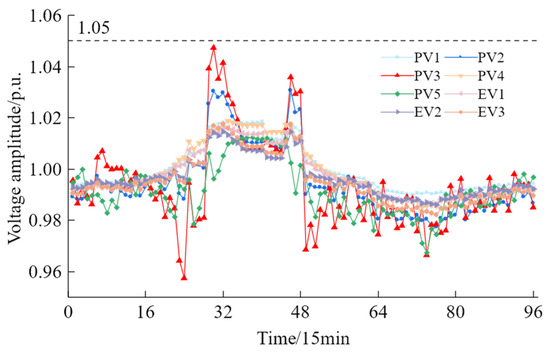
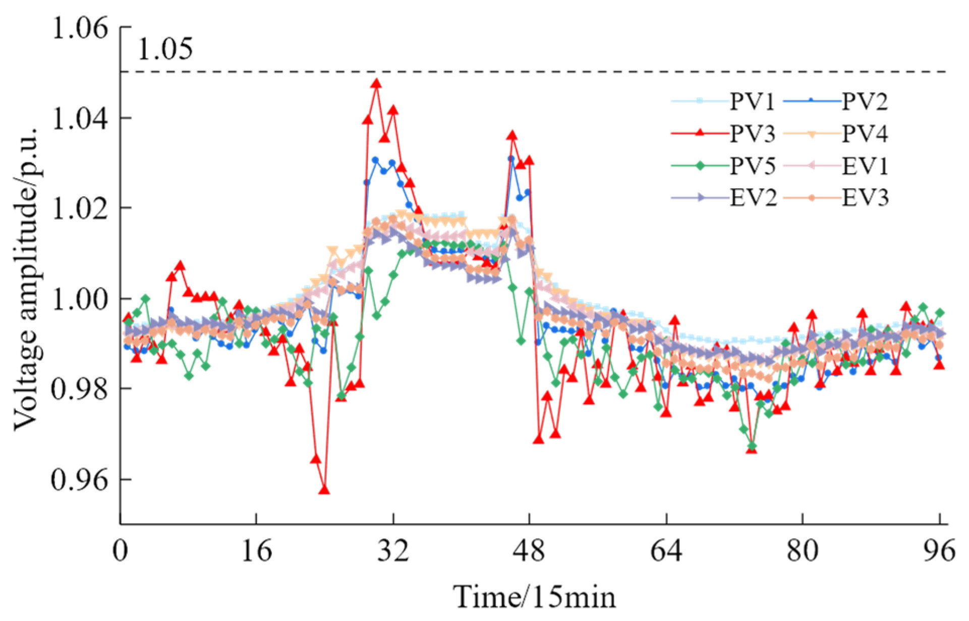
Source-load connection buses are strongly affected by variations in PV output and EV charging demand, resulting in pronounced voltage fluctuations. These buses are selected to evaluate the voltage-regulation performance of the GAT during representative periods. Bus voltages before and after optimization are shown in Figure 9 and Figure 10.

Figure 9. Voltages at source-load connection buses before optimization.

Figure 10. Voltages at source-load connection buses after optimization.

Before optimization, the source-load connection buses exhibit pronounced voltage fluctuations and risk violating the voltage limits. At 11:00, high PV generation increases power injection and drives several bus voltages above 1.05 p.u. Around the evening peak at 19:00, PV output falls to zero while the base load and EV charging demand increase, causing substantial voltage drops; some PV and EV connection buses approach 0.92 p.u. After applying the reactive power decisions generated by the GAT, these fluctuations are mitigated. Midday overvoltage is suppressed, with all bus voltages remaining below 1.05 p.u. During the evening peak, undervoltage is alleviated, and PV and EV connection-bus voltages rise above 0.95 p.u., with some reaching approximately 0.98 p.u. These results demonstrate coordinated voltage regulation under stochastic source-load fluctuations in the simulated network.

4.3.3. Spatiotemporal Distribution of System Voltage

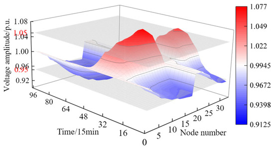
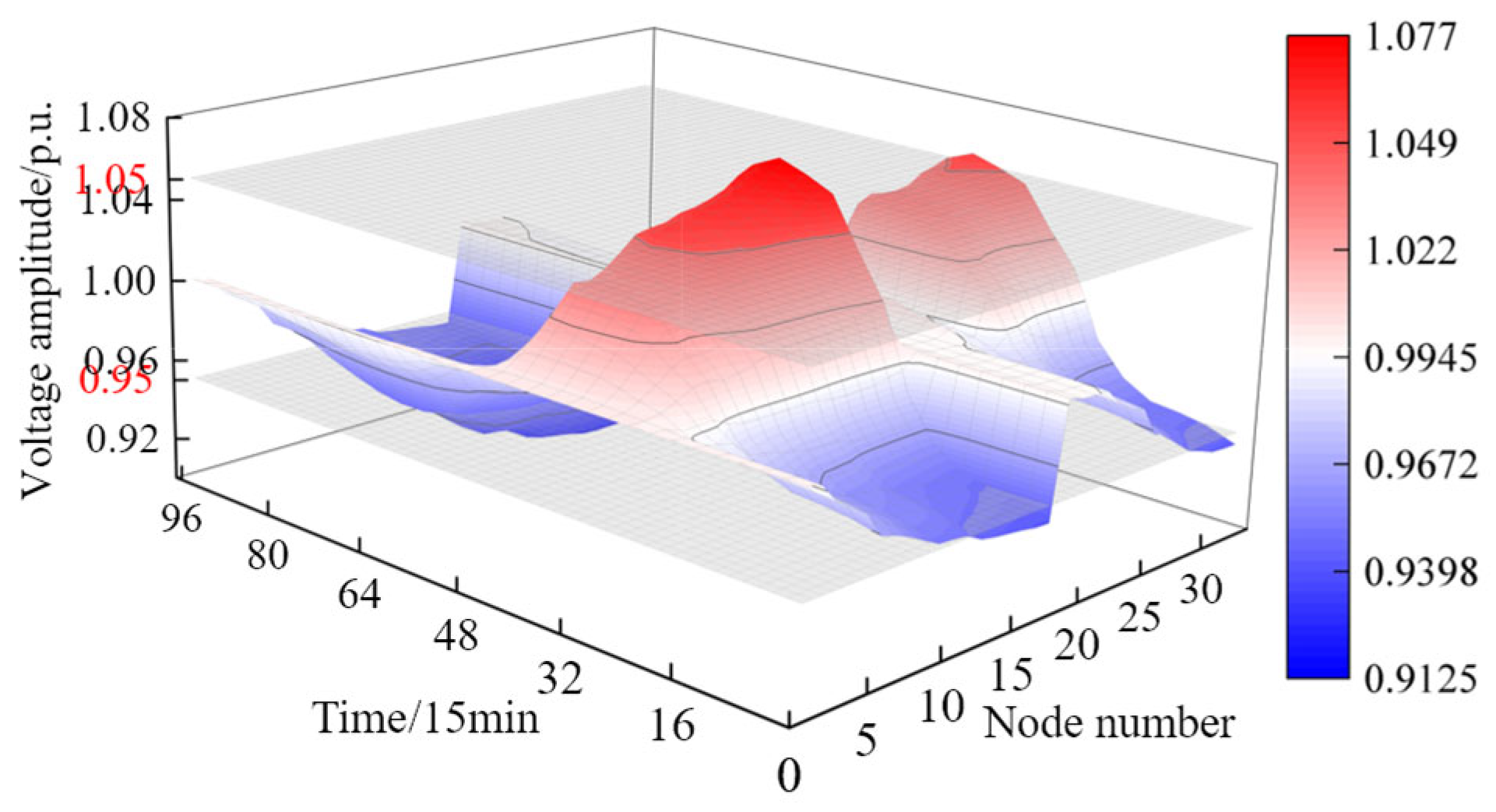
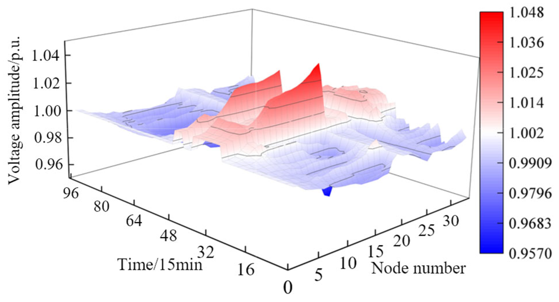
We further analyzed the spatiotemporal distribution of system voltage. The voltage of every bus throughout the day before and after optimization is shown in Figure 11 and Figure 12.

Figure 11. Spatiotemporal distribution of system voltage before optimization.

Figure 12. Spatiotemporal distribution of system voltage after optimization.

Before optimization, bus voltages fluctuate substantially across time and space. The maximum voltage is 1.077 p.u., whereas the minimum is 0.9125 p.u., indicating an uneven voltage profile and a pronounced peak-to-valley difference. After GAT optimization, all bus voltages are controlled within 0.95–1.05 p.u., eliminating voltage-limit violations. The voltage distribution also becomes more concentrated and the voltage profile smoother, indicating more coordinated reactive power regulation across the network. For clarity, the vertical-axis limits are set to 0.92–1.08 p.u. in Figure 11 and 0.95–1.05 p.u. in Figure 12 to cover the respective data ranges.

Overall, the proposed data-driven reactive power optimization model substantially reduces computation time while preserving optimization performance. The IEEE 33-bus simulation demonstrates the computational feasibility of rapid online decision-making for distribution network regulation.

4.3.4. Validation of the PSO-Derived Labels

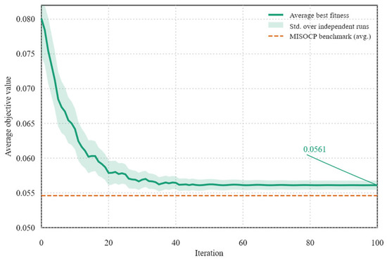
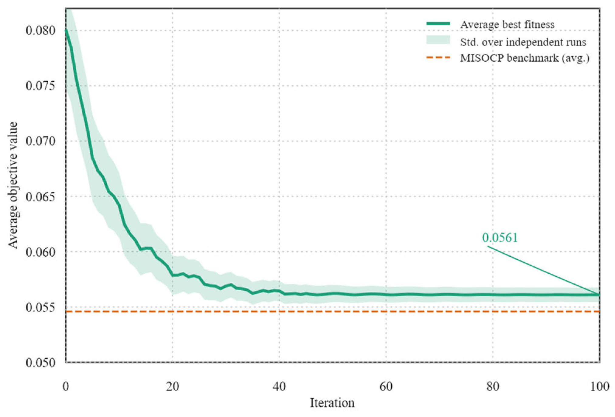
To assess the quality of the PSO-derived labels used for training, 20 representative operating conditions are additionally solved using a convexified mixed-integer second-order cone (MISOCP) benchmark implemented in Gurobi, and the resulting objective values are compared with the PSO labels in Table 4. The MISOCP benchmark provides a tractable convex reference for the original nonlinear, nonconvex reactive power optimization problem; it is therefore used as an independent benchmark rather than as a fully equivalent replacement for the original PSO formulation. The convergence of the average best fitness is shown in Figure 13.

Table 4. Comparison between the PSO-derived labels and the convex MISOCP benchmark.

Metric	PSO	MISOCP Benchmark	Relative Gap (%)
Average objective value	0.0561	0.0546	2.8
Maximum objective gap (%)	--	--	4.1
Average computation time (s)	83.7667	0.6	--

Figure 13. Convergence of the average best fitness of the PSO algorithm over representative operating conditions.

The MISOCP formulation replaces the original nonlinear and nonconvex power-flow constraints with a convexified second-order-cone representation that can be solved efficiently by Gurobi. Its shorter computation time and lower objective value in Table 4 therefore reflect the properties of the convex benchmark formulation and should not be interpreted as a direct speed or optimality comparison for the original PSO problem. The PSO is retained for full annual label generation because it directly handles the original mixed discrete-continuous optimization problem and the proposed multi-time-scale variable-update strategy across all 35,040 operating snapshots. The MISOCP formulation is applied only to representative operating conditions for an independent assessment of the PSO-derived labels.

4.3.5. Ablation Study and Comparison with Recent Methods

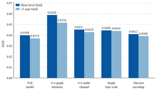
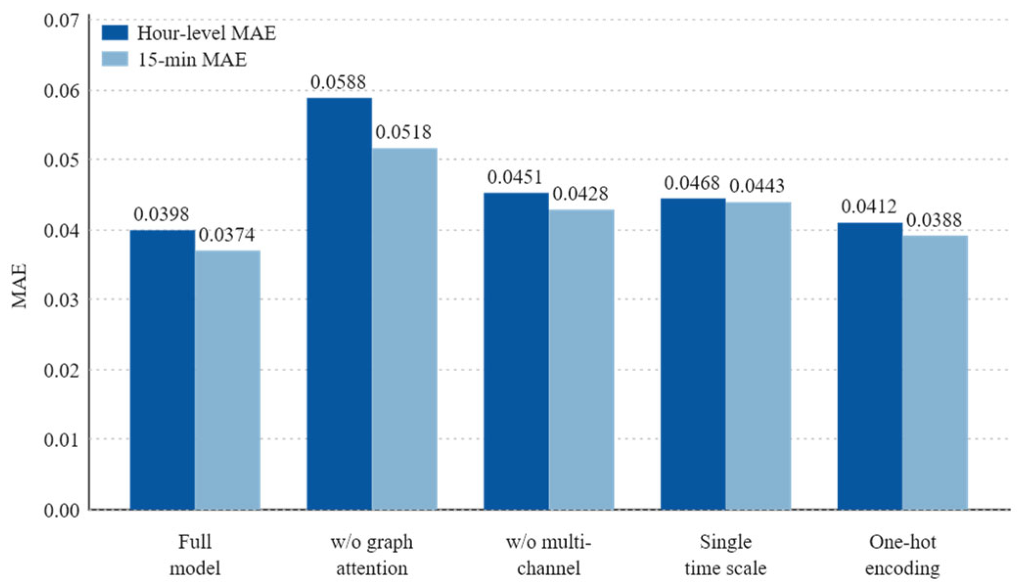
To isolate the contribution of each component, the graph-attention mechanism is replaced by a fixed-adjacency GCN, the multi-channel architecture is replaced by a single shared channel, the two-time-scale formulation is replaced by a single 15 min model, and the continuous encoding of discrete variables is replaced by one-hot encoding. The resulting performance is summarized in Table 5 and shown in Figure 14. Removing graph attention increases the hour-level MAE from 0.0398 to 0.0588, the single-channel variant to 0.0451, and the single-scale variant to 0.0468, whereas replacing the continuous encoding mainly increases the discrete-control error (MDCE) from 0.0412 to 0.0703.

Table 5. Ablation study of the proposed framework.

Variant	Hour MAE	Hour RMSE	Hour MDCE	15 Min MAE	15 Min RMSE
Full model (proposed GAT)	0.0398	0.0407	0.0412	0.0374	0.0397
w/o graph attention (fixed-adjacency GCN)	0.0588	0.0678	0.0638	0.0518	0.0624
w/o multi-channel architecture	0.0451	0.0509	0.0476	0.0428	0.0481
Single time-scale (15 min only)	0.0468	0.0522	0.0501	0.0443	0.0497
One-hot encoding of discrete variables	0.0412	0.0425	0.0703	0.0388	0.0410

Figure 14. Ablation study of the proposed framework at the hour-level and 15 min time scales.

The proposed method is also compared with a recent graph-based optimization method [8], which achieves an hour-level MAE/RMSE of 0.0487/0.0552; the proposed GAT remains more accurate at the hour level under the same test protocol.

4.4. Robustness Analysis

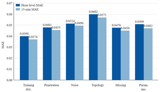
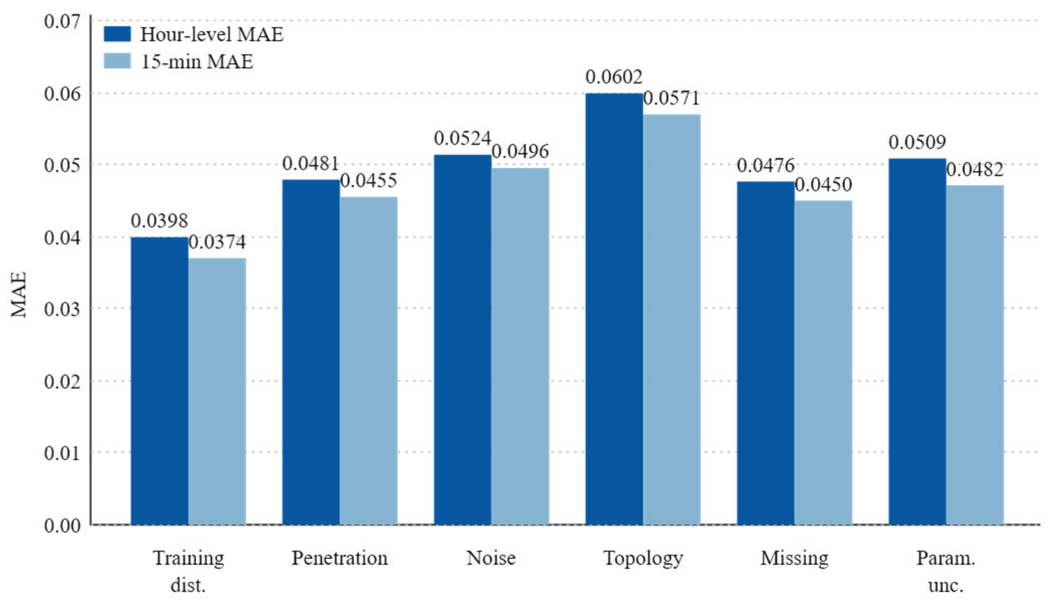
To assess robustness outside the training distribution, the trained GAT is evaluated under the following conditions: (1) PV and EV penetration levels changed to 30% and 25%, respectively; (2) Gaussian measurement noise with standard deviations of 0.5% and 1.0% added to the inputs; (3) single-line outages of branches 6–7 and 8–9; (4) random missing measurements at 5% of the buses; and (5) ±10% uncertainty in the line and load parameters. Here, the PV and EV penetration levels are implemented by scaling the aggregate PV generation and EV charging-load profiles relative to the corresponding base-load level, and the 0.5%/1.0% noise levels denote the standard deviations of zero-mean Gaussian noise normalized by the corresponding input-variable magnitudes. Table 6 summarizes the results, and Figure 15 visually compares the corresponding prediction errors at both time scales. Accuracy degrades gradually as the operating conditions move away from the training distribution, while a high proportion of intervals remains voltage-feasible, indicating acceptable robustness under moderate deviations.

Table 6. Robustness of the proposed GAT under out-of-distribution conditions.

Scenario	Hour MAE	Hour RMSE	15 Min MAE	15 Min RMSE	Voltage-Feasible (%)
Training distribution	0.0398	0.0407	0.0374	0.0397	100
PV/EV penetration 30%/25%	0.0481	0.0562	0.0455	0.0531	98.7
Measurement noise (0.5%/1.0%)	0.0524	0.0608	0.0496	0.0581	96.5
Topology change (line outage)	0.0602	0.0715	0.0571	0.0684	94.2
Missing measurements (5%)	0.0476	0.0554	0.0450	0.0527	97.8
Parameter uncertainty (±10%)	0.0509	0.0593	0.0482	0.0566	96.9

Figure 15. Robustness of the Proposed GAT under Out-of-Distribution Conditions at the Hour-Level and 15-Min Time Scales.

4.5. Additional Generalization Validation

The preceding experiments evaluate the learning accuracy, regulation performance, and robustness of the proposed framework under the primary sample-level random split. To supplement these results with an assessment of performance across a continuous time period, an additional chronological-block validation is conducted using test data that are not used during training.

The annual operating sequence is divided by complete months. The data from the first nine months are used for training, whereas the data from the subsequent three months are reserved as an independent test block. The same GAT architecture, hyperparameters, PSO-derived labels, and evaluation metrics are used as in the primary experiment. No samples from the test block are used during model training.

The results are summarized in Table 7. The random-split results characterize performance under the primary sample-level validation protocol, whereas the chronological-block results assess performance on an entirely unseen continuous time period. Under the chronological-block split, the hour-level model achieves an MAE/RMSE/MDCE of 0.0446/0.0489/0.0468, and the 15 min model achieves an MAE/RMSE of 0.0421/0.0455. Although the errors are higher than those obtained with the random split, the model maintains useful control-decision prediction accuracy on the unseen time block.

Table 7. Model performance under random-split and chronological-block validation.

Validation Protocol	Hour-Level MAE	Hour-Level RMSE	Hour-Level MDCE	15-Min MAE	15-Min RMSE
Random 9:1 split	0.0398	0.0407	0.0412	0.0374	0.0397
Chronological-block split	0.0446	0.0489	0.0468	0.0421	0.0455

This additional validation complements the primary learning and regulation analyses and indicates that the proposed framework retains useful performance when evaluated under a chronological data partition.

5. Conclusions

To address the complexity of reactive power optimization and the limited suitability of conventional methods for online implementation in active distribution networks with high penetration of emerging resources, including DG and EVs, we propose a multi-time-scale GAT-based online optimization and control method. The main conclusions are as follows:

(1)

A PSO-based multi-time-scale reactive power optimization method is developed. A time-scale-dependent variable-update strategy coordinates discrete and continuous control variables, while rolling optimization over successive operating snapshots generates a PSO-derived control-decision dataset that captures the relationship between operating states and control decisions. The annual dataset contains 35,040 operating snapshots with a 15 min resolution.

(2)

A GAT-based online decision-making model is developed for active distribution networks. By learning the nonlinear mapping from distribution network operating states to PSO-derived control decisions, the model replaces online iterative optimization with forward inference. The average GAT inference time is 0.0703 s, compared with 83.7667 s for the PSO. The hour-level MAE/RMSE values are 0.0398/0.0407, whereas the 15 min MAE/RMSE values are 0.0374/0.0397. The proposed model therefore balances online inference speed and prediction accuracy.

(3)

A two-level GAT-based online decision-making model operating at hour-level and 15 min time scales is developed. The model coordinates discrete control devices and continuous reactive power resources hierarchically, supporting rapid regulation in the simulated system under source-load fluctuations. In the typical-day case, the average network loss is 0.2331 MW, the average voltage deviation is 0.9512%, and all bus voltages are maintained within 0.95–1.05 p.u. These results correspond to the tested operating distribution; robustness under larger out-of-distribution deviations and field application remain to be further validated.

References

- Sun, X.; Qiu, J.; Zhao, J. Real-Time Volt/Var Control in Active Distribution Networks With Data-Driven Partition Method. IEEE Trans. Power Syst. 2021, 36, 2448–2461. [Google Scholar] [CrossRef] [Scilit]
- Cao, D.; Zhao, J.; Hu, W.; Ding, F.; Yu, N.; Huang, Q.; Chen, Z. Model-Free Voltage Control of Active Distribution System With PVs Using Surrogate Model-Based Deep Reinforcement Learning. Appl. Energy 2022, 306, 117982. [Google Scholar] [CrossRef] [Scilit]
- Kayacık, S.E.; Kocuk, B. An MISOCP-Based Solution Approach to the Reactive Optimal Power Flow Problem. IEEE Trans. Power Syst. 2021, 36, 529–532. [Google Scholar] [CrossRef] [Scilit]
- Zhang, T.; Yu, L.; Yue, D.; Dou, C.; Xie, X.; Hancke, G.P. Two-Timescale Coordinated Voltage Regulation for High Renewable-Penetrated Active Distribution Networks Considering Hybrid Devices. IEEE Trans. Ind. Inform. 2024, 20, 3456–3467. [Google Scholar] [CrossRef] [Scilit]
- Li, S.; Wu, W.; Lin, Y. Robust Data-Driven and Fully Distributed Volt/VAR Control for Active Distribution Networks With Multiple Virtual Power Plants. IEEE Trans. Smart Grid 2022, 13, 2627–2638. [Google Scholar] [CrossRef] [Scilit]
- Peng, H.; Liao, K.; Yang, J.; Pang, B.; He, Z. Deep Reinforcement Learning Based Multi-Timescale Volt/Var Control in Distribution Networks Considering Network Reconfiguration. IEEE Trans. Sustain. Energy 2025, 16, 2948–2958. [Google Scholar] [CrossRef] [Scilit]
- Sun, X.; Qiu, J.; Zhao, J. Optimal Local Volt/Var Control for Photovoltaic Inverters in Active Distribution Networks. IEEE Trans. Power Syst. 2021, 36, 5756–5766. [Google Scholar] [CrossRef] [Scilit]
- Lopez-Garcia, T.B.; Domínguez-Navarro, J.A. Optimal Power Flow With Physics-Informed Typed Graph Neural Networks. IEEE Trans. Power Syst. 2025, 40, 381–393. [Google Scholar] [CrossRef] [Scilit]
- Hu, D.; Ye, Z.; Gao, Y.; Ye, Z.; Peng, Y.; Yu, N. Multi-Agent Deep Reinforcement Learning for Voltage Control With Coordinated Active and Reactive Power Optimization. IEEE Trans. Smart Grid 2022, 13, 4873–4886. [Google Scholar] [CrossRef] [Scilit]
- Cao, D.; Zhao, J.; Hu, W.; Ding, F.; Huang, Q.; Chen, Z.; Blaabjerg, F. Data-Driven Multi-Agent Deep Reinforcement Learning for Distribution System Decentralized Voltage Control With High Penetration of PVs. IEEE Trans. Smart Grid 2021, 12, 4137–4150. [Google Scholar] [CrossRef] [Scilit]
- Nellikkath, R.; Chatzivasileiadis, S. Physics-Informed Neural Networks for AC Optimal Power Flow. Electr. Power Syst. Res. 2022, 212, 108412. [Google Scholar] [CrossRef] [Scilit]
- Liu, H.; Wu, W.; Wang, Y. Bi-Level Off-Policy Reinforcement Learning for Two-Timescale Volt/VAR Control in Active Distribution Networks. IEEE Trans. Power Syst. 2023, 38, 385–395. [Google Scholar] [CrossRef] [Scilit]
- Veličković, P.; Cucurull, G.; Casanova, A.; Romero, A.; Liò, P.; Bengio, Y. Graph Attention Networks. In Proceedings of the 6th International Conference on Learning Representations (ICLR), Vancouver, BC, Canada, 30 April–3 May 2018. [Google Scholar] [CrossRef] [Scilit]
- Sun, X.; Qiu, J.; Tao, Y.; Zhao, J. Data-Driven Combined Central and Distributed Volt/Var Control in Active Distribution Networks. IEEE Trans. Smart Grid 2023, 14, 1855–1867. [Google Scholar] [CrossRef] [Scilit]
- Huang, W.; Pan, X.; Chen, M.; Low, S.H. DeepOPF-V: Solving AC-OPF Problems Efficiently. IEEE Trans. Power Syst. 2022, 37, 800–803. [Google Scholar] [CrossRef] [Scilit]
- Yan, R.; Xing, Q.; Xu, Y. Multi-Agent Safe Graph Reinforcement Learning for PV Inverters-Based Real-Time Decentralized Volt/Var Control in Zoned Distribution Networks. IEEE Trans. Smart Grid 2024, 15, 299–311. [Google Scholar] [CrossRef] [Scilit]
- Yang, Q.; Wang, G.; Sadeghi, A.; Giannakis, G.B.; Sun, J. Two-Timescale Voltage Control in Distribution Grids Using Deep Reinforcement Learning. IEEE Trans. Smart Grid 2020, 11, 2313–2323. [Google Scholar] [CrossRef] [Scilit]
- Long, Y.; Kirschen, D.S. Bi-Level Volt/VAR Optimization in Distribution Networks With Smart PV Inverters. IEEE Trans. Power Syst. 2022, 37, 3604–3613. [Google Scholar] [CrossRef] [Scilit]
- Xu, R.; Zhang, C.; Xu, Y.; Dong, Z.; Zhang, R. Multi-Objective Hierarchically-Coordinated Volt/Var Control for Active Distribution Networks With Droop-Controlled PV Inverters. IEEE Trans. Smart Grid 2022, 13, 998–1011. [Google Scholar] [CrossRef] [Scilit]
- Chen, Z.; Cai, S.; Meliopoulos, A.P.S. Robust Deep Reinforcement Learning for Volt-VAR Optimization in Active Distribution System Under Uncertainty. IEEE Trans. Smart Grid 2025, 16, 4463–4474. [Google Scholar] [CrossRef] [Scilit]
- Li, P.; Wu, Z.; Zhang, C.; Xu, Y.; Dong, Z.; Hu, M. Multi-Timescale Affinely Adjustable Robust Reactive Power Dispatch of Distribution Networks Integrated With High Penetration of PV. J. Mod. Power Syst. Clean Energy 2023, 11, 324–334. [Google Scholar] [CrossRef] [Scilit]
- Cao, D.; Zhao, J.; Hu, J.; Pei, Y.; Huang, Q.; Chen, Z.; Hu, W. Physics-Informed Graphical Representation-Enabled Deep Reinforcement Learning for Robust Distribution System Voltage Control. IEEE Trans. Smart Grid 2024, 15, 233–246. [Google Scholar] [CrossRef] [Scilit]
- Yang, T.; Guo, Y.; Deng, L.; Sun, H.; Wu, W. A Linear Branch Flow Model for Radial Distribution Networks and Its Application to Reactive Power Optimization and Network Reconfiguration. IEEE Trans. Smart Grid 2021, 12, 2027–2036. [Google Scholar] [CrossRef] [Scilit]
- Sun, X.; Qiu, J. A Customized Voltage Control Strategy for Electric Vehicles in Distribution Networks With Reinforcement Learning Method. IEEE Trans. Ind. Inform. 2021, 17, 6852–6863. [Google Scholar] [CrossRef] [Scilit]
- Pan, X.; Chen, M.; Zhao, T.; Low, S.H. DeepOPF: A Feasibility-Optimized Deep Neural Network Approach for AC Optimal Power Flow Problems. IEEE Syst. J. 2023, 17, 673–683. [Google Scholar] [CrossRef] [Scilit]
Disclaimer/Publisher’s Note: The statements, opinions and data contained in all publications are solely those of the individual author(s) and contributor(s) and not of MDPI and/or the editor(s). MDPI and/or the editor(s) disclaim responsibility for any injury to people or property resulting from any ideas, methods, instructions or products referred to in the content. |
© 2026 by the authors. Licensee MDPI, Basel, Switzerland. This article is an open access article distributed under the terms and conditions of the Creative Commons Attribution (CC BY) license.