Prioritizing Beijing Subway Intervals for Field Review Using PS-InSAR and SBAS-InSAR

Abstract

Railway and metro inspection planning requires an ordered set of engineering intervals for follow-up investigation. This study combines persistent scatterer interferometric synthetic aperture radar (PS-InSAR) and small baseline subset interferometric synthetic aperture radar (SBAS-InSAR) to prioritize intervals by joint relative prominence and assess ranking uncertainty. The Shilihe–Bagou corridor of Beijing Subway Line 10 was analyzed using 48 ascending Sentinel-1A scenes from 2021 to 2024. Rates were centered on each product’s corridor median and aggregated into paired route bins. The smaller method-specific percentile rank defined joint prominence, while paired block bootstrap quantified rank variability. PS-only and SBAS-only rankings shared only two of their first five intervals. The joint same-direction shortlist comprised the two Huoqiying–Bagou units, Changchunqiao–Huoqiying, Cishousi–Chedaogou, and Lianhuaqiao–Gongzhufen. Spatial and representation tests retained four or five baseline members, and all three boundary-allocation tests retained all five. The main Huoqiying–Bagou interval had a baseline 95% rank interval of 1–3 and, together with Changchunqiao–Huoqiying, remained selected throughout the tested spatial settings. The short open-cut Huoqiying–Bagou unit remained prominent but changed to opposite relative directions under the 200 m grid. These results distinguish persistent priorities for targeted field review from intervals requiring closer examination of spatial sampling and cross-method differences.

1. Introduction

Time-series interferometric synthetic aperture radar (InSAR) provides repeated observations of surface displacement across extensive infrastructure networks [1,2]. Applications to metro systems and railways have demonstrated its value for identifying deformation patterns and locating potential anomalies [3,4]. Transport-monitoring studies also show that the usefulness of these observations depends on the observation conditions [5]. For inspection and maintenance planning, a deformation map must be linked to named engineering units and a manageable set of follow-up tasks. Macchiarulo et al. [6] addressed this interface by integrating InSAR measurements with infrastructure inventories in a geographic information system (GIS). An interval-level review order can support this workflow by directing limited inspection resources toward locations where the observations warrant closer examination.

Persistent scatterer interferometry (PS-InSAR) estimates deformation from temporally stable radar targets [7,8]. Small baseline subset interferometry (SBAS-InSAR) instead organizes observations through a network of short-baseline interferograms [9,10]. Differences in target selection and network construction can produce different spatial sampling and local rate estimates [11]. Processing-chain comparisons therefore examine agreement across products rather than assuming identical observations [12,13]. For engineering screening, these differences matter because an interval can appear prominent in one product and ordinary in the other. A shared interval representation is needed before their relative prominence can be combined.

Comparisons with Global Navigation Satellite System (GNSS) and leveling observations assess the accuracy of InSAR displacement estimates [14,15]. Such external measurements also support interpretation of metro-station deformation and tunneling responses [16,17]. Applications to geotechnical design compliance [18], construction-induced movement [19], and metro deformation patterns [20] extend this evidence toward engineering assessment.

Turning deformation observations into a review order requires identifying both the relevant signals and the engineering units to which they belong. Target characterization [21], time-series clustering [22], and integration with geospatial information [23] distinguish deformation behaviors; railway-tunneling frameworks organize such observations for settlement management [24]. A remaining practical question is how to select intervals for follow-up when two InSAR products assign different prominence to the same corridor. A single-product list reflects one processing chain, while a deformation map alone does not specify an order for reviewing engineering units. The present study addresses this selection step by combining method-specific prominence and testing whether the resulting priorities persist under changes in spatial representation.

Spatial support refers here to the area or route length over which observations are aggregated. Deformation varies across the Beijing Plain [25], and changing aggregation units can alter statistical relationships through the modifiable areal unit effect [26,27]. We therefore compare the products on common grid cells and fixed route bins before ranking engineering intervals. Using the Shilihe–Bagou section of Beijing Subway Line 10, we first compare the joint-prominence shortlist with single-product and mean-percentile rankings. We then examine whether the leading intervals persist under alternative spatial settings and boundary assignments. Paired resampling describes variation in their ranks. The outputs identify where field review should begin and where spatial sampling or cross-method differences require further examination.

2. Case Study and Data

2.1. Study Area, Data, and Engineering Intervals

The case study covers approximately 30.7 km of the Shilihe–Bagou section of Beijing Subway Line 10 within a 500 m buffer on either side of the route. Engineering records define 29 intervals, including station-to-station, station-to-vent-shaft, and open-cut sections. Their identifiers and chainages define the field-review units. The engineering boundaries include small overlaps between intervals 13 and 14 and between intervals 28 and 29. These management units are preserved in the analysis, allowing their spatial overlap to be considered when planning field visits.

A priority review interval is defined here by the prominence of its relative surface-deformation signal in both InSAR products. The analysis produces an ordered list of these engineering units together with information on their shared observations and rank variation.

The input dataset comprises 48 ascending Sentinel-1A interferometric wide-swath single-look complex scenes acquired during 2021–2024. Sentinel-1’s mission characteristics are described by the European Space Agency [28]. The same acquisition period, precise orbit products, digital elevation model (DEM), and study extent were used for the two processing chains. Their geocoded outputs contain mean line-of-sight (LOS) deformation rates and associated quality fields.

2.2. InSAR Processing and Quality Control

PS-InSAR and SBAS-InSAR were processed independently in SARscape 5.6.2. Table 1 documents the acquisition networks, filtering, unwrapping, inversion, atmospheric correction, and output-screening settings. Both chains used AUX_POEORB precise orbit products and the Shuttle Radar Topography Mission (SRTM) 3 arcsec DEM, conventionally described as approximately 90 m. The archived DEM header records a spacing of 0.0008333333° in both geographic coordinates. This DEM was an input to the completed InSAR processing chains, where it supported topographic-phase correction and geocoding; it is not the spatial resolution of the deformation measurements. Each product retained its internal reference during time-series processing. A corridor-relative reference was subsequently applied for interval comparison.

Table 1. Processing and output-screening settings for the two InSAR products.

Item	Persistent Scatterer InSAR (PS-InSAR)	Small Baseline Subset InSAR (SBAS-InSAR)
Common inputs	48 ascending Sentinel-1A IW-SLC scenes; 2021–2024; AUX_POEORB precise orbits; SRTM 3 arcsec DEM (approximately 90 m)	Same as PS-InSAR
Software	SARscape 5.6.2	SARscape 5.6.2
Image network	Master scene on 14 March 2023; 47 master–slave interferometric pairs	Perpendicular baseline ≤ 15%; temporal baseline ≤ 180 days; ≤8 consecutive scenes per connection; 191 differential interferometric pairs
Co-registration and interferometry	Orbit initialization; correlation threshold, 0.25; precise co-registration SNR threshold, 3.2	Range/azimuth multilooking 4/1; correlation threshold, 0.25; precise co-registration SNR threshold, 3.2
Filtering and unwrapping	Phase stability estimated using the PS time-series workflow	Goldstein filtering (window 32; overlap 80%); MCF–Delaunay unwrapping; first/second unwrapping coherence thresholds, 0.15/0.30
Time-series inversion	Velocity search, −25 to 25 mm yr−1 (step 1); residual-height search, −70 to 70 m (step 2)	Linear deformation model; Jacobi–SVD inversion; first- and second-order inversion coherence thresholds, both 0.15
Atmospheric correction	Spatial low-pass scale, 1200 m; temporal high-pass scale, 365 days	Spatial low-pass scale, 1600 m; temporal high-pass scale, 365 days
Reference and refinement	Reference-area parameters: coherence precision of 0.75 and mean PS count of 200; no external refinement GCP file was introduced	Automatic orbit refinement and re-flattening; no external refinement GCP file was introduced
Output screening	Final coherence threshold, 0.50; geocoded output interval, 15 m	Height precision threshold, 10 m; velocity precision threshold, 8 mm yr−1; temporal coherence threshold, 0.10
Valid points	283,989	118,155

The present analysis uses these completed products as its inputs. Although a finer SRTM 1 arcsec product is available, the upstream processing was not repeated with that DEM. The effect of changing DEM resolution is therefore distinct from the common-grid and route-bin sensitivity tests reported here and has not been quantified.

The PS network used the scene on 14 March 2023 as its master and comprised 47 master–slave pairs. The SBAS connection settings specified a 15% perpendicular-baseline limit, a 180-day temporal-baseline limit, and a maximum of eight consecutive scenes per connection, yielding 191 interferometric pairs. The percentage baseline limit is reported in the native SARscape parameter form. The two products were screened using the settings listed in Table 1 before spatial aggregation.

The archived point products also contain the software-reported velocity-precision field, Vprecision. For points inside the 500 m corridor buffer, its median and interquartile range are 0.530 and 0.437–0.607 mm yr⁻¹ for PS-InSAR (283,173 points), and 1.037 and 0.806–1.360 mm yr⁻¹ for SBAS-InSAR (118,155 points). These summaries describe internal point-level precision estimates. The SBAS velocity precision threshold of 8 mm yr⁻¹ in Table 1 is an output-screening limit, not the achieved accuracy of an interval rate. Spatial dependence and the shared reference prevent these point-level quantities from being treated directly as uncertainty bounds for the aggregated interval medians.

2.3. Spatial Coordinates and Engineering Boundaries

The common-grid dataset uses a local metric representation of geographic coordinates centered at 116.36198° E, 39.86399° N. Longitude and latitude offsets are converted using 111,320 cos(39.86399°) and 110,540 m per degree, respectively. For route projection, the representative coordinates supplied with the common-cell data are converted to Gauss–Krüger coordinates with a central meridian of 117° E and a false easting of 500,000 m, consistent with the engineering polyline. Chainage is the cumulative polyline distance to the nearest projected point, measured from the Shilihe end of the analyzed route.

Engineering boundaries are maintained at their original numerical precision during calculation and reported to 0.001 km. Interval 1 begins approximately 18 m before the route origin because the engineering and route chainage origins differ slightly. A fixed route bin belongs to an interval whenever their chainage ranges intersect. This rule retains partially intersecting boundary bins and permits a bin to belong to more than one engineering interval.

The spatial procedure provides two linked units: common grid cells for matching the two products and route bins for representing engineering intervals. Table 1 documents the input processing and quality-control settings. The interval statistics and their roles in ranking are defined below. The resulting interval values, names, and chainages are presented for comparison with engineering records.

3. Methods

3.1. Shared Spatial Support and Assessment Workflow

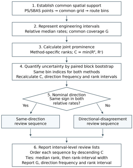
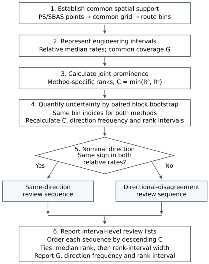
The assessment follows the workflow in Figure 1. Mean point rates are calculated separately for PS-InSAR and SBAS-InSAR within 100 m × 100 m cells. Cells containing both products constitute the common-grid population. The median of each product over that population is subtracted from its cell rates, establishing a corridor-relative reference. Common cells are then assigned to 100 m route bins; the median cell rate within each bin provides one paired observation for interval aggregation. This sequence gives each retained bin equal weight in the interval representative rate.

Figure 1. Workflow for interval representation, common-prominence assessment, paired resampling, and generation of the two review sequences.

The 100 m × 100 m grid and the 100 m route bins serve different purposes. The grid provides a shared areal unit for products with different target distributions; the bins provide repeated along-route observations within the engineering boundaries. The intervals span approximately 0.18–2.20 km, so the baseline represents most units with multiple bins while retaining the short open-cut units. These dimensions define the aggregation scale, not the spatial resolution of the original radar measurements or the size of a structural defect. Their effect on interval selection is examined using alternative grid and bin sizes in Section 3.4 and reported in Section 4.4.

$${\tilde{v}}_i^m=v_i^m-median\left(v_k^m\right),k\in commoncells.$$

Interval prioritization is based on joint prominence C, defined as the smaller of the two method-specific percentile ranks. Common coverage G records the fraction of expected route bins containing paired observations. Paired block bootstrap yields the resampled same-direction frequency Pdir and a rank interval U. Nominal direction separates same-direction and directional-disagreement review sequences, each ordered by C. The bootstrap median rank and rank-interval width resolve exact ties in C. Coverage and uncertainty accompany the resulting order as distinct information for field planning.

3.2. Metric Definitions

Let v_i^m denote the mean LOS rate in common grid cell i for method m, where P and S identify as PS-InSAR and SBAS-InSAR. The corridor-relative cell rate is obtained by subtracting the median over all common cells. Within each route bin, these centered cell rates are aggregated by their median. Table 2 defines the interval statistics using u_β^m for the resulting paired bin rates and V_j for the set of valid bins in interval j. The distinction between a cell, a route bin, and an engineering interval is maintained throughout the calculation.

Table 2. Definitions, interpretation, and use of the interval-level statistics.

Statistic	Definition	Value and Interpretation	Role
Representative relative rate	${\tilde{v}}_j^m=median(u_b^m:b\in V_j)$	Median paired bin rate; sign is relative to the corridor reference.	Basis for prominence and direction.
Method-specific percentile rank	$R_j^m={\displaystyle \frac{rank\left(\right|{\tilde{v}}_j^m\left|\right)}{N}}$	Ascending average rank divided by N; 1/N to 1. Larger values indicate greater within-method prominence.	Common relative scale for the two products.
Joint prominence	$C_j=min(R_j^P,R_j^S)$	Larger C requires larger percentile ranks in both products.	Sets the nominal order.
Nominal direction	$D_j=I({\tilde{v}}_j^P{\tilde{v}}_j^S>0)$	1: Same sign; 0: opposite signs or a zero rate. No zero representative rates occur in this case.	Separates the two review sequences.
Common coverage	$G_j={\displaystyle \frac{n_{valid,j}}{n_{expected,j}}}$	0–1; fraction of expected bins containing paired observations.	Reports shared spatial support.
Resampled same-direction frequency	$P_{dir,j}={\displaystyle \frac{1}{B}}{\sum }_{b=1\dots B}{D}_j^{\left(b\right)}$	0–1; near 1: consistently same direction; near 0: consistently different direction; intermediate values: varying direction.	Reports directional stability.
Rank interval and width	$U_j=[Q_{0.025}(r_j),Q_{0.975}(r_j)]$ $U_{R,j}=U_{j,upper}-U_{j,lower}$	Empirical 95% range of bootstrap ranks; smaller width indicates less rank variation.	Reports ranking uncertainty and breaks exact C ties after median rank.

The absolute value is taken after calculating the interval median. Thus, an absolute representative rate is the magnitude of a corridor-relative rate, not a rate measured against an externally fixed datum. Percentile ranks are calculated separately for the two methods across all 29 intervals, with average ranks for ties. This definition makes C large when both products assign an interval a high relative position. Table 2 also defines the nominal direction D from the signs of the relative rates.

Notations: m ∈ {P, S}; j indexes engineering intervals; V_j contains their valid route bins; N = 29. The indicator I equals 1 when its condition holds and 0 otherwise. D_j^(b) is D recalculated in bootstrap resample b. Q denotes an empirical quantile of the B = 1000 resampled ranks. R uses ascending average ranks; r uses descending competition ranks of C.

3.3. Paired Along-Route Block Bootstrap

To represent local dependence among neighboring bins, we use moving-block resampling following the block-bootstrap principle of Künsch [29]. Valid bins are arranged in route order within each interval. The baseline block contains two adjacent bins (200 m). Candidate starts are sampled with replacement from the available internal positions until the original number of valid bins is reached; excess indices are truncated without circular wraparound. The same sampled indices are applied to both products. Intervals with fewer than four valid bins use paired one-bin resampling. With 1000 resamples and random seed 20260713, all interval representative rates, method-specific percentile ranks, and C values are recalculated. In every resample, C is ranked in descending order across all 29 intervals, with tied values receiving the minimum occupied rank. The nearest observed 2.5th and 97.5th rank percentiles define U, and the nearest observed 50th percentile defines the median rank. Pdir is the fraction of resamples in which the two interval representative rates have the same sign. Resampling is performed within each interval; the resulting intervals describe rank variability conditional on the observed route-bin series.

The two-bin baseline resamples contiguous pairs rather than treating all neighboring bins as independent. At the baseline bin size, it preserves the observed pairing and local ordering within each 200 m block while allowing more resampling combinations than longer blocks in short engineering intervals. It is a working resampling scale, not an estimated spatial correlation length. The one-, two-, and three-bin comparison in Section 4.4 examines sensitivity to this choice. The paired one-bin fallback preserves cross-method pairing where too few bins are available for the baseline blocks. The resulting rank intervals quantify variability conditional on the available observations and the specified resampling scheme; they are not an independent validation of the priority order.

3.4. Ranking Comparisons and Sensitivity Tests

Four ranking rules are compared on the same 29 intervals: PS percentile rank, SBAS percentile rank, their arithmetic mean, and their minimum C. The first five positions under each rule form a fixed-shortlist-size comparison. We report the selected interval identities and their overlap, using the baseline tie-breaking order for exact score ties. All four rules use the absolute value of the signed interval median and the same centered paired observations.

Design sensitivity is evaluated by changing one setting at a time. The tested common-grid sizes are 60, 100, 150, and 200 m; the route-bin sizes are 50, 100, 150, and 200 m. Interval amplitude is represented by the absolute median, median absolute value, or absolute mean. Each setting is compared with the 100 m grid, 100 m bins, and absolute-median baseline. Representative rates, C, nominal direction, and paired bootstrap statistics are recalculated. The intervals are then assigned to the same-direction or directional-disagreement sequence and ordered using the rule below. We compare the first five members of each sequence with its baseline list. Spearman correlation of C across all 29 intervals and the unfiltered top-five list provide overall ranking diagnostics. Bootstrap block lengths of one, two, and three bins are compared through rank-interval widths. Intervals with fewer than four valid bins retain paired one-bin resampling.

Boundary sensitivity is tested with three alternative assignments: retain a bin when its representative chainage lies inside the interval; allocate an intersecting bin exclusively to the interval with the greatest overlap length; omit every bin shared by multiple intervals. Representative chainage is the median chainage of the common cells in that bin. Largest-overlap ties are resolved by interval identifier. These alternatives respectively test partially intersecting bins, unique allocation, and the contribution of shared observations. Signed medians, percentile ranks, C, and the paired bootstrap are recalculated for each assignment with the same settings as the baseline.

The same-direction sequence contains intervals with D = 1, meaning that the two signed corridor-relative representative rates have the same sign. The directional-disagreement sequence contains intervals with D = 0. In this dataset, these intervals have opposite signs; no representative rate is zero. A sequence is an ordered list of engineering intervals, not a temporal deformation sequence. Nominal D determines list membership, whereas Pdir describes the frequency of same-sign rates under resampling.

Within each sequence, intervals are sorted by descending C, then by ascending bootstrap median rank and ascending rank-interval width. Any remaining tie is displayed by interval identifier. G and Pdir are reported alongside this order without additional weighting or a coverage threshold. An interval without any paired bins has no defined representative rate and is reported as inevaluable. All 29 intervals in the present case contain paired bins.

Python 3 (https://www.python.org/, accessed on 22 September 2026) scripts implement spatial aggregation, interval ranking, paired resampling, and plotting from the InSAR products and engineering records. The scripts and derived analysis inputs are provided in the Supplementary Materials.

4. Results

4.1. Spatial Observations and Interval Representation

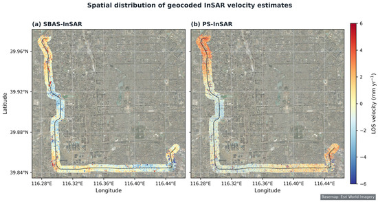
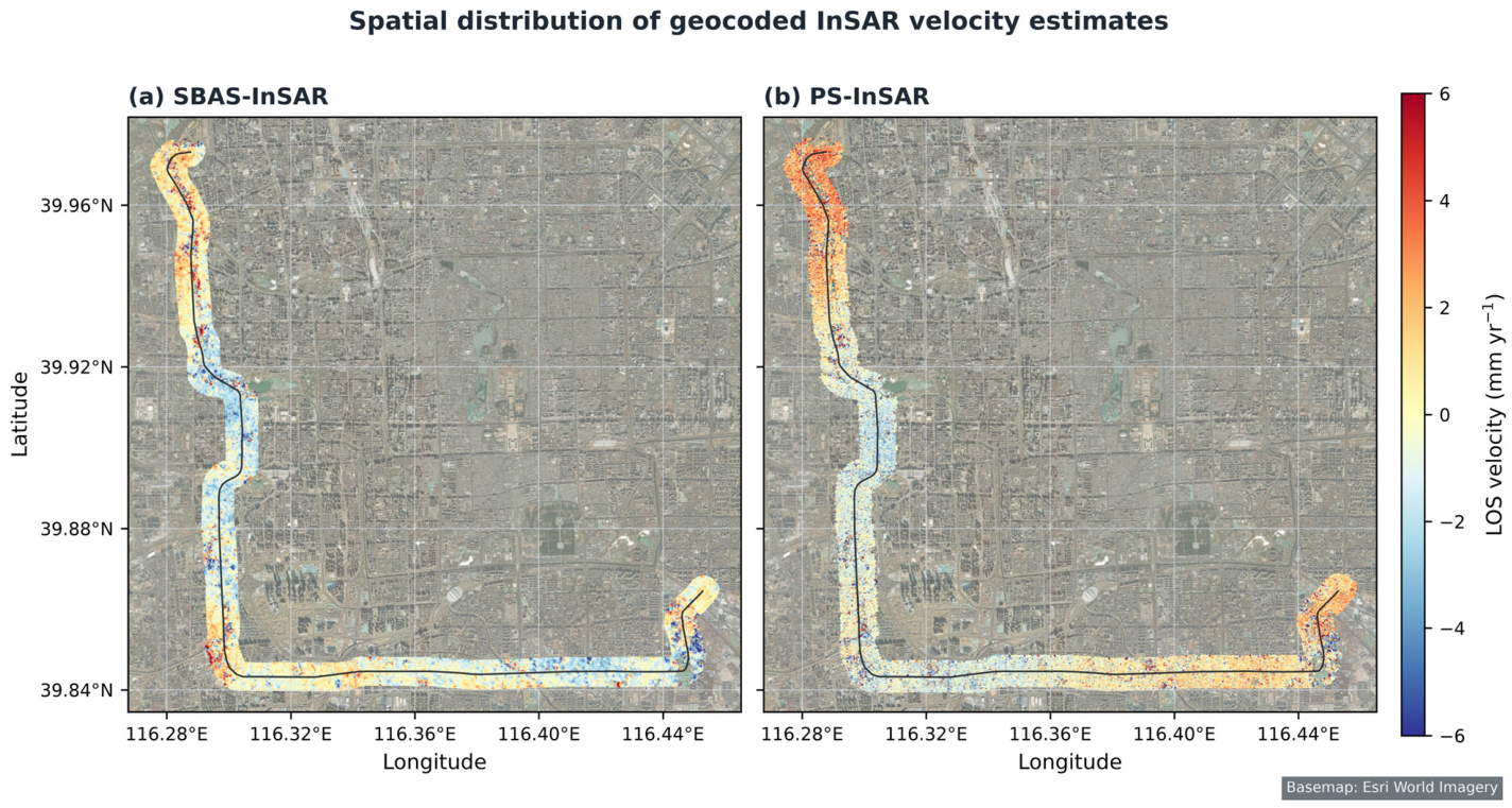
The geocoded products contain 283,989 PS points and 118,155 SBAS points. Their spatial distributions are shown in Figure 2. The 100 m common grid contains 2877 cells. Mapping route bins to the 29 engineering intervals yields 295 expected interval–bin memberships, of which 294 contain valid paired observations. These valid memberships represent 288 distinct bins; six boundary bins are each associated with two intervals. The single unfilled membership is the bin immediately before the route origin in interval 1.

Figure 2. Mean LOS deformation rates from (a) SBAS-InSAR and (b) PS-InSAR in the study corridor. The common color range describes the geocoded products before corridor-median centering. The route is overlaid on Esri World Imagery.

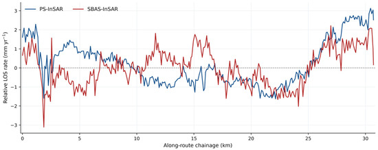
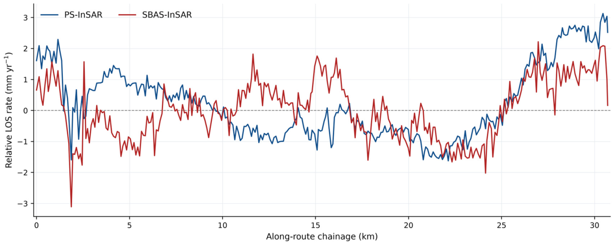
After corridor-median centering and route aggregation, the profiles retain both shared and contrasting spatial patterns (Figure 3). The northern intervals from Cishousi toward Bagou have positive relative representative rates in both products, while the Lianhuaqiao–Gongzhufen interval has negative relative rates in both. In the Songjiazhuang–Shiliuzhuang interval, the representative rates have opposite signs. These contrasts carry through to the interval-level prominence and direction statistics.

Figure 3. Corridor-relative LOS rates in fixed 100 m route bins. Each product is centered by its median over the common-grid population before route aggregation. The zero line denotes that relative reference.

4.2. Joint Prominence and Comparison with Alternative Rankings

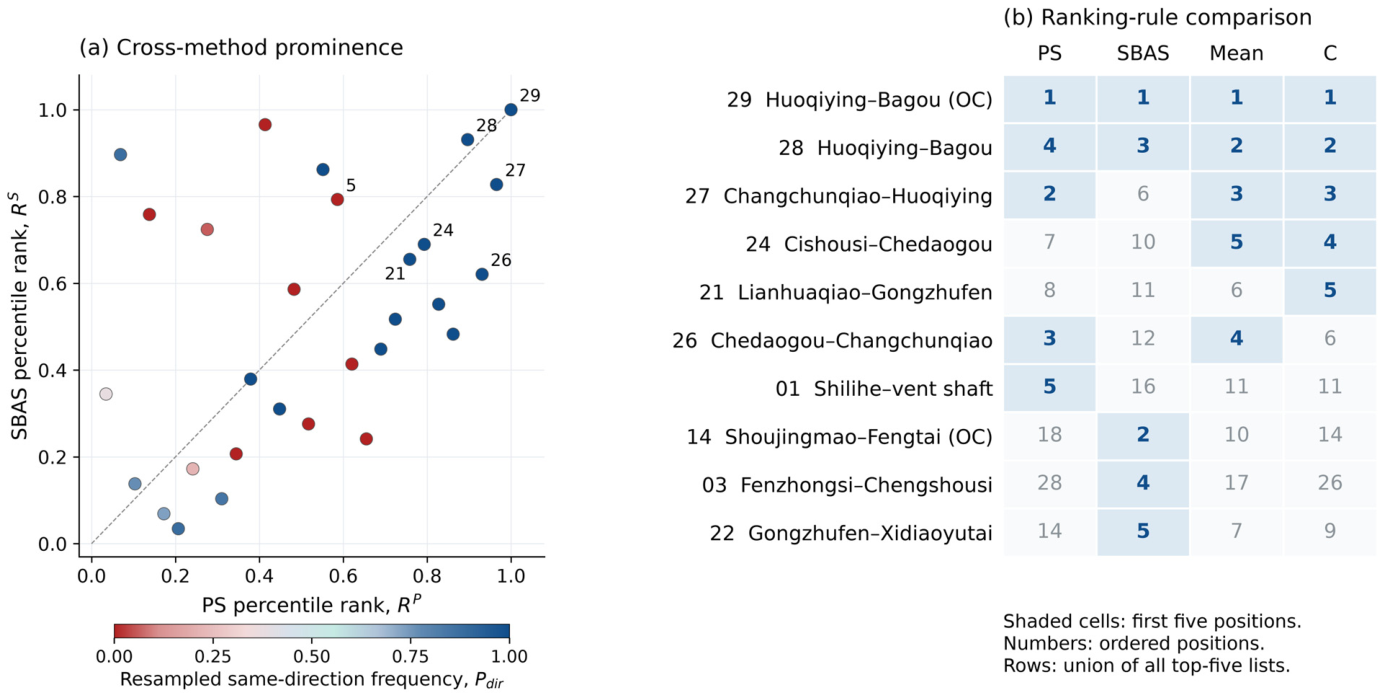
Intervals 29, 28, 27, 24, and 21 have the five largest C values and the same nominal relative direction in both products. Their C values are 1.000, 0.897, 0.828, 0.690, and 0.655, respectively. The magnitudes of the corridor-relative representative rates are 3.040/2.074 mm yr⁻¹ for interval 29 and 2.317/1.403 mm yr⁻¹ for interval 28 (PS/SBAS). Interval 21 is also jointly prominent, with signed relative rates of −1.466 and −1.017 mm yr⁻¹. These negative values indicate positions below the respective corridor medians, rather than independently verified absolute subsidence. The common-prominence ranking therefore includes both signs of deviation from the corridor reference.

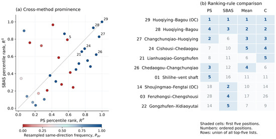
PS-only ranking selects intervals 29, 27, 26, 28, and 1, whereas SBAS-only ranking selects 29, 14, 28, 3, and 22. Only the two Huoqiying–Bagou units, 29 and 28, occur in both lists. Mean-percentile ranking gives 29, 28, 27, 26, and 24. Relative to that list, C moves interval 21 into the top five and interval 26 to sixth place (Figure 4). The PS/SBAS percentile ranks are 0.759/0.655 for interval 21 and 0.931/0.621 for interval 26, so the minimum-percentile rule favors the former despite the larger PS rank of the latter.

Figure 4. Joint prominence and alternative ranking rules. (a) Method-specific percentile ranks for all 29 intervals; joint prominence C is the smaller coordinate. Colors represent the resampled same-direction frequency Pdir, from 0 to 1. (b) Ordered positions under PS-only, SBAS-only, mean-percentile, and minimum-percentile ranking. Rows contain the union of the four top-five lists; shaded cells identify selected positions. Exact score ties use the same secondary ordering as the baseline. OC denotes open-cut.

Interval 5, Songjiazhuang–Shiliuzhuang, has C = 0.586 with signed rates of 0.871 and −1.179 mm yr⁻¹. It is the highest-C member of the directional-disagreement sequence. Full signed rates and directional classifications are reported in Table 3.

Table 3. Interval-level rates, prominence, coverage, direction, and bootstrap ranking results.

Engineering Interval (ID)	Chainage (km)	PS/SBAS (mm yr−1)	RP/Rs	C	V/E	G	D	Pdir	Rank/Median [95% Range]
Shilihe–Vent Shaft (1)	−0.018–0.685	1.761/0.659	0.862/0.483	0.483	7/8	0.875	1	1.000	11/10 [3–19]
Vent Shaft–Fenzhongsi (2)	0.700–1.579	1.611/0.784	0.828/0.552	0.552	9/9	1.000	1	0.999	8/8 [3–22]
Fenzhongsi–Chengshousi (3)	1.787–2.606	−0.120/−1.398	0.069/0.897	0.069	10/10	1.000	1	0.877	26/25 [19–28]
Chengshousi–Songjiazhuang (4)	2.775–4.316	0.914/−0.540	0.621/0.414	0.414	17/17	1.000	0	0.000	14/15 [10–22]
Songjiazhuang–Shiliuzhuang (5)	4.538–5.575	0.871/−1.179	0.586/0.793	0.586	11/11	1.000	0	0.000	7/8 [5–12]
Shiliuzhuang–Dahongmen (6)	5.730–6.814	0.751/−0.389	0.517/0.276	0.276	12/12	1.000	0	0.000	18/17 [10–23]
Dahongmen (OC)–Jiaomendong (7)	7.036–7.960	0.443/0.071	0.310/0.103	0.103	10/10	1.000	1	0.849	24/25 [21–28]
Jiaomendong–Jiaomenxi (8)	8.166–9.179	0.344/−0.134	0.241/0.172	0.172	11/11	1.000	0	0.217	22/22 [18–28]
Jiaomenxi–Caoqiao (9)	9.386–10.846	−0.226/−0.049	0.172/0.069	0.069	16/16	1.000	1	0.731	26/26 [22–28]
Caoqiao–Jijiamiao (10)	11.084–12.415	−0.732/0.865	0.483/0.586	0.483	15/15	1.000	0	0.000	11/13 [9–18]
Jijiamiao–Shoujingmao (11)	12.636–13.590	−0.932/0.336	0.655/0.241	0.241	10/10	1.000	0	0.000	20/19 [12–22]
Shoujingmao (OC)–Fengtai (12)	13.725–14.077	−0.301/−0.031	0.207/0.034	0.034	4/4	1.000	1	0.886	28/22 [18–28]
Shoujingmao–Fengtai (13)	14.083–14.924	−0.597/0.254	0.345/0.207	0.207	10/10	1.000	0	0.000	21/21 [13–26]
Shoujingmao–Fengtai (OC) (14)	14.909–15.253	−0.712/1.548	0.414/0.966	0.414	4/4	1.000	0	0.000	14/11 [5–17]
Fengtai–Niwa (15)	15.457–15.897	−0.351/1.071	0.276/0.724	0.276	5/5	1.000	0	0.062	18/21 [15–26]
Fengtai–Niwa (OC) (16)	15.897–16.278	−0.220/1.076	0.138/0.759	0.138	5/5	1.000	0	0.000	23/21 [5–26]
Niwa–Xiju (OC) (17)	16.451–16.986	−0.004/0.455	0.034/0.345	0.034	6/6	1.000	0	0.380	28/28 [25–28]
Xiju–Liuliqiao (OC) (18)	17.140–18.611	−0.718/−0.409	0.448/0.310	0.310	16/16	1.000	1	1.000	17/17 [11–22]
Liuliqiao–Lianhuaqiao (19)	18.746–20.744	−0.698/−0.491	0.379/0.379	0.379	21/21	1.000	1	1.000	16/15 [10–21]
Liuliqiao–Lianhuaqiao (OC) (20)	20.746–20.939	−1.343/−0.544	0.690/0.448	0.448	3/3	1.000	1	1.000	13/14 [10–28]
Lianhuaqiao–Gongzhufen (21)	21.129–21.980	−1.466/−1.017	0.759/0.655	0.655	9/9	1.000	1	1.000	5/5 [3–16]
Gongzhufen–Xidiaoyutai (22)	22.176–24.374	−0.826/−1.337	0.552/0.862	0.552	23/23	1.000	1	1.000	8/9 [5–17]
Xidiaoyutai–Cishousi (23)	24.543–25.576	−0.129/−0.109	0.103/0.138	0.103	11/11	1.000	1	0.769	24/24 [19–28]
Cishousi–Chedaogou (24)	25.770–27.211	1.478/1.059	0.793/0.690	0.690	16/16	1.000	1	1.000	4/5 [2–12]
Chedaogou (OC)–Changchunqiao (25)	27.376–27.653	1.454/0.687	0.724/0.517	0.517	4/4	1.000	1	1.000	10/11 [5–15]
Chedaogou–Changchunqiao (26)	27.657–28.405	2.349/0.916	0.931/0.621	0.621	9/9	1.000	1	1.000	6/6 [2–11]
Changchunqiao–Huoqiying (27)	28.620–29.233	2.654/1.192	0.966/0.828	0.828	7/7	1.000	1	1.000	3/3 [2–7]
Huoqiying–Bagou (28)	29.508–30.470	2.317/1.403	0.897/0.931	0.897	10/10	1.000	1	1.000	2/2 [1–3]
Huoqiying–Bagou (OC) (29)	30.448–30.630	3.040/2.074	1.000/1.000	1.000	3/3	1.000	1	1.000	1/1 [1–7]

V/E denotes valid/expected bin memberships; D = 1 denotes the same nominal relative direction. Rates retain their signs and are rounded to 0.001 mm yr⁻¹ for numerical reporting; this rounding does not specify measurement accuracy or precision. Rank and rank intervals refer to the full set of 29 intervals; rank 1 is the highest. OC denotes open-cut. Table values and all plots use the same centered common-grid and route-bin data.

4.3. Shared Coverage, Ranking Uncertainty, and Priority Lists

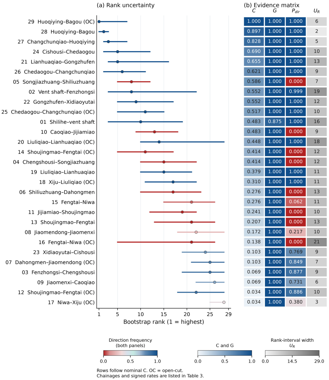
Common coverage G ranges from 0.875 to 1.000, with a median of 1.000; a total of 28 intervals have complete bin coverage. The nominal rates have the same sign in 18 intervals and opposite signs in 11. Pdir ranges from 0.000 to 1.000 and equals 1.000 for all five leading intervals. Interval 5 retains opposite signs in every resample (Pdir = 0.000), whereas some lower-prominence intervals show intermediate frequencies, including intervals 8 and 17 (0.217 and 0.380).

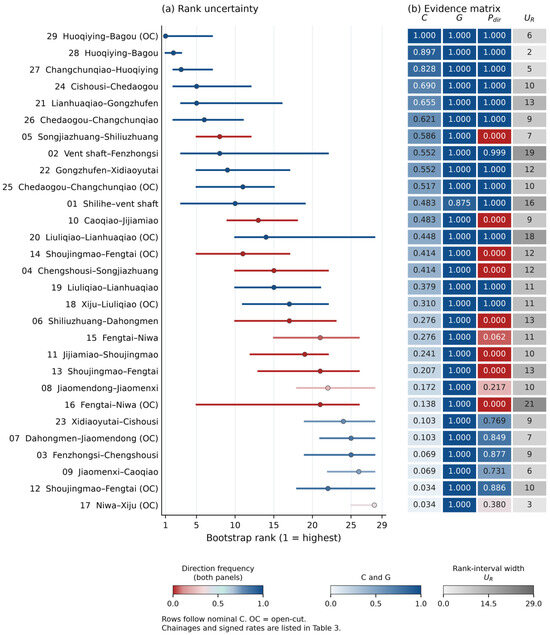
The bootstrap median ranks of intervals 29, 28, and 27 are one, two, and three, with 95% rank intervals of 1–7, 1–3, and 2–7, respectively (Figure 5). Interval 28 has the narrowest range among these leading intervals. Intervals 24 and 21 both have a median rank of five, with ranges of 2–12 and 3–16. The nominal ordering is consequently clearer than the separation of their resampled ranks. Interval 5 has a median rank of eight and a range of 5–12 across the full set of 29 intervals.

Figure 5. Bootstrap rankings and evidence indicators. (a) Median ranks and 95% rank intervals across all 29 intervals; rank 1 is the highest. Colors represent the resampled same-direction frequency Pdir. (b) Joint prominence C, common coverage G, Pdir, and rank-interval width U_R. The rows follow descending C, with ties resolved by median rank and width. C, G, and Pdir range from 0 to 1; U_R is expressed in rank positions. Separate continuous legends distinguish Pdir, the C/G columns, and U_R. OC denotes an open-cut interval.

Applying the stated ordering rule gives the same-direction sequence beginning with intervals 29, 28, 27, 24, and 21. The directional-disagreement sequence begins with intervals 5, 10, 14, and 4. The baseline top three same-direction intervals span Changchunqiao–Huoqiying and the two Huoqiying–Bagou engineering units. Table 3 retains the original identifiers and chainages so that these statistical results can be matched to field records.

4.4. Sensitivity to Spatial Settings and Boundary Assignment

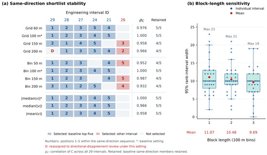
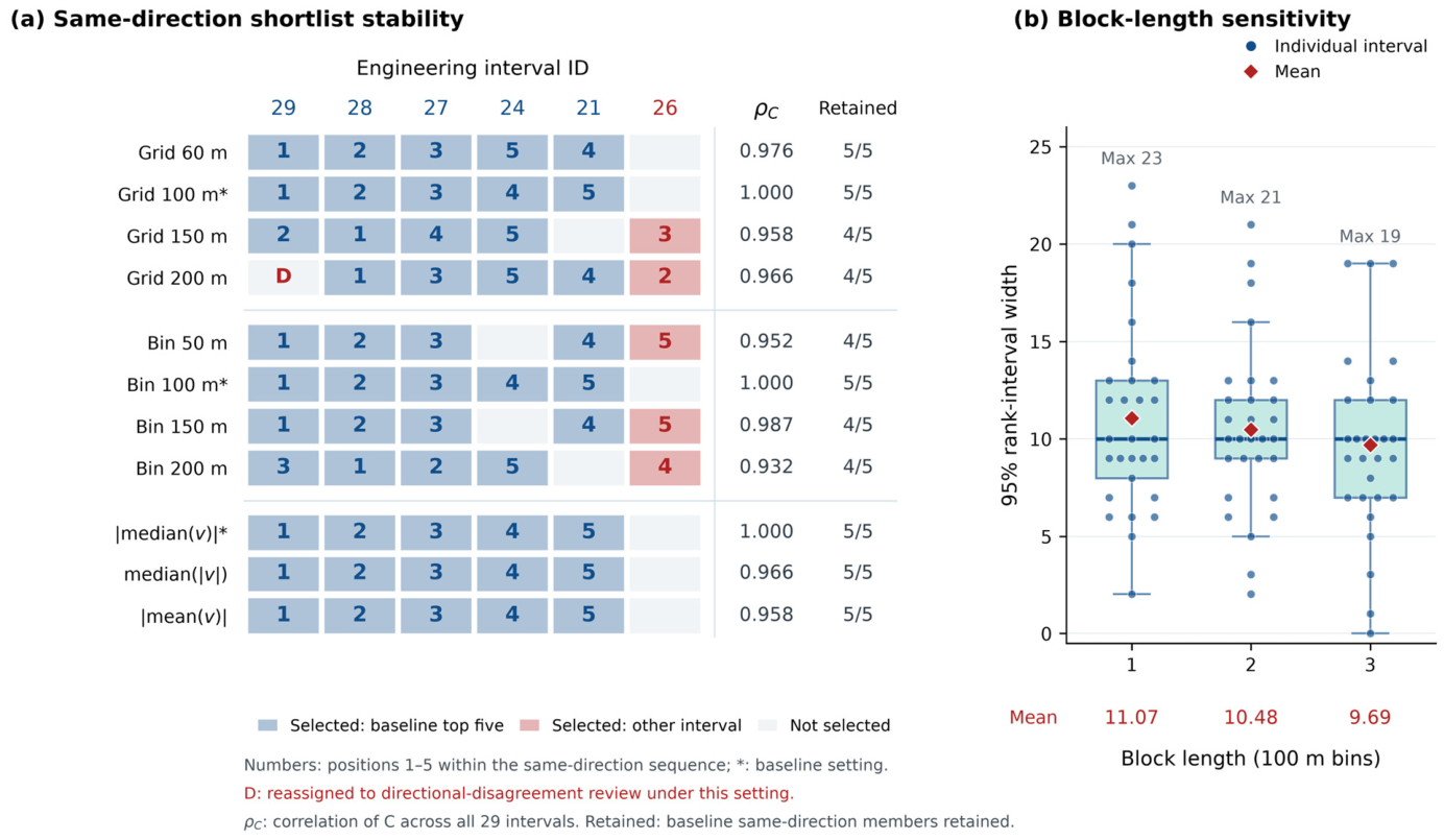
The same-direction shortlist retains four or five of its baseline members across the design tests (Figure 6a). Huoqiying–Bagou (28) and Changchunqiao–Huoqiying (27) remain in this shortlist throughout. The 150 m grid gives the sequence 28, 29, 26, 27, and 24; the 200 m grid gives 28, 26, 27, 21, and 24. In the latter setting, the short Huoqiying–Bagou open-cut unit (29) retains high joint prominence (C = 0.828), but its representative PS and SBAS rates are 1.732 and −1.151 mm yr⁻¹. It therefore moves to the directional-disagreement sequence. Across all 29 intervals, C’s correlations with the baseline range from 0.932 to 1.000.

Figure 6. Sensitivity of the same-direction review shortlist and ranking uncertainty. (a) Ordered positions among the first five same-direction intervals after recalculating direction and ranking for each setting. Blue cells identify selected baseline members; red cells identify other selected intervals, and gray cells indicate non-selection. D marks a unit reassigned to directional-disagreement review. The adjacent columns report C’s correlation across all 29 intervals and retention of baseline same-direction members; asterisks mark baseline settings. (b) Rank-interval widths for all 29 engineering intervals. Boxes span the 25th–75th percentiles; lines denote medians, and whiskers extend to observations within 1.5 interquartile ranges. Dots show individual intervals and red diamonds show means. Intervals with fewer than four bins retain one-bin resampling.

Using the median absolute rate or the absolute mean rate gives correlations of 0.966 and 0.958 with the absolute-median baseline and retains all five baseline same-direction shortlist members. Changing block length from one to three bins reduces the mean rank-interval width from 11.07 to 9.69 and the maximum width from 23 to 19 (Figure 6b). The baseline two-bin case has a mean width of 10.48; the median width is 10 for all three block lengths. The directional-disagreement shortlist also retains four or five baseline members across all settings. Songjiazhuang–Shiliuzhuang (5) remains in its first two positions. Full results for both sequences and the unfiltered ranking are provided in the Supplementary Materials.

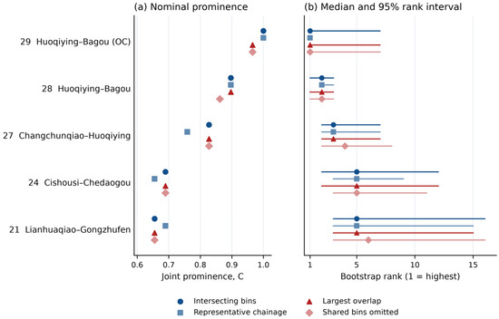
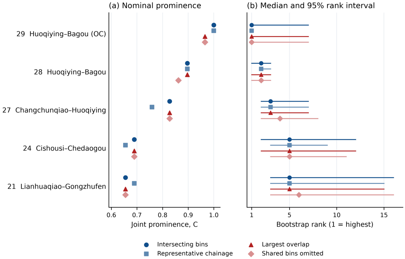
All three boundary assignments retain the baseline same-direction top-five membership (Figure 7). C’s correlations with the baseline are 0.987 for representative-chainage inclusion, 1.000 for largest-overlap allocation, and 0.980 when shared bins are omitted. Representative-chainage inclusion exchanges the fourth and fifth positions, giving 29, 28, 27, 21, and 24; the other two assignments retain 29, 28, 27, 24, and 21. No interval changes its nominal directional classification. The alternatives contain 265, 288, and 282 valid interval–bin memberships, respectively.

Figure 7. Boundary-allocation sensitivity for the five leading baseline intervals. (a) Recalculated C. (b) Median ranks and 95% rank intervals from paired resampling across all 29 units. Symbols distinguish the baseline and three allocation rules. A point without a visible line denotes an interval with coincident rank quantiles. OC denotes open-cut.

The Huoqiying–Bagou main interval (28) retains a median rank of two and a 95% range of 1–3 or 2–3 in every boundary test. The short open-cut interval (29) retains first place but is represented by two bins rather than three in each alternative. Its range becomes 1–1 under representative-chainage inclusion and remains 1–7 under both largest-overlap allocation and removal of shared bins. Complete results for all 29 intervals are provided in the Supplementary Materials.

5. Discussion

5.1. Effects of the Joint Criterion on Interval Selection

The ranking comparison shows why using two InSAR products changes the field-review list. PS-only and SBAS-only screenings share just two of their first five units, both at Huoqiying–Bagou. Their agreement identifies an immediate common focus, but their other selections differ. Combining the product-specific ranks retains that focus and brings Changchunqiao–Huoqiying into the leading group. This result connects the processing differences examined in cross-method comparisons [12,13] to a concrete management outcome: the set of engineering intervals selected at a fixed shortlist size.

The comparison with mean-percentile ranking clarifies the specific role of C. Averaging allows a high rank in one product to offset a lower rank in the other, whereas the minimum requires both to support the resulting prominence. Chedaogou–Changchunqiao illustrates this distinction: its PS percentile is 0.931 but its SBAS percentile is 0.621. Lianhuaqiao–Gongzhufen has a lower PS percentile of 0.759 and a higher SBAS percentile of 0.655, and therefore enters the top five of joint prominence. The two rules express different screening objectives. Mean-percentile ranking emphasizes combined relative magnitude; C emphasizes the level reached by both products. For a list intended to identify commonly expressed deformation signals, the latter provides a direct selection criterion. The component ranks preserve the stronger single-product signals for subsequent examination.

5.2. The Persistent Core and the Shortlist Boundary

Huoqiying–Bagou (28) and Changchunqiao–Huoqiying (27) form a persistent same-direction review core across the tested spatial settings. Their repeated selection supports retaining them at the start of the proposed field-review program. The short Huoqiying–Bagou open-cut unit remains prominent in both products, but its direction class changes under the 200 m grid. This unit merits attention alongside the main interval, with an initial check of target distribution and aggregation near its boundaries. Cishousi–Chedaogou and Lianhuaqiao–Gongzhufen lie nearer the shortlist boundary and may be replaced when aggregation changes. Their inclusion should therefore be considered alongside the bin-level profiles and existing engineering records, rather than decided from one nominal rank alone.

The boundary tests strengthen this interpretation. Assigning shared bins to one interval or omitting them altogether retains all five baseline same-direction units, and inclusion by representative chainage only exchanges the fourth and fifth positions. The leading group therefore persists after duplicated boundary contributions are removed. The larger changes under 150–200 m grids arise from changes in spatial aggregation across the corridor, consistent with the modifiable areal unit effect [26,27]. Shared coverage is nearly complete in this case, with G = 1.000 in 28 intervals, so its principal role is to document the observational basis of the ranking. The sensitivity results then identify where that ranking responds to the choice of spatial support.

5.3. Using Rank Uncertainty to Plan the Leading Review Group

Nominal prominence and rank stability contribute different information to the first field visits. The open-cut Huoqiying–Bagou unit has the highest baseline C, while the main Huoqiying–Bagou interval has the most concentrated leading baseline rank interval, at 1–3. The latter remains within ranks 1–3 or 2–3 across all three boundary tests and stays in the same-direction shortlist across the spatial settings. A coordinated visit to these nearby engineering units can therefore combine review of a stable common-direction target with examination of the short open-cut unit’s aggregation-sensitive direction. Retaining the original interval identifiers supports record matching. The baseline includes six bins shared by two intervals, whereas exclusive largest-overlap allocation and omission of shared bins leave 288 and 282 valid interval–bin memberships, respectively. Both alternatives retain the same five leading same-direction intervals. These tests separate statistical duplication at boundaries from the coordination of field visits.

The short open-cut unit shows why the number of observations must accompany a rank interval. Its representative-chainage assignment retains two similar paired observations and produces a rank of one in every resample; the other boundary assignments give a range of 1–7. The concentrated result reflects the limited combinations available from those two observations. Increasing block length from one to three bins reduces the observed mean rank-interval width from 11.07 to 9.69, with 10.48 for the two-bin baseline. Longer blocks restrict the available resampling combinations within short intervals. A narrow range in this setting describes conditional resampling stability, not independent confirmation of the deformation signal. For field planning, overlapping rank intervals support reviewing a leading group together, while small bin counts identify locations where additional spatial observations could improve discrimination among priorities.

5.4. Matching Follow-Up Tasks to the Observed Signals

The same-direction and directional-disagreement sequences guide different initial checks. The leading same-direction intervals have prominent relative representative rates of the same sign in both products. For the persistent Huoqiying–Bagou and Changchunqiao–Huoqiying intervals, the proposed first step is to match the chainages in Table 3 to inspection records and available deformation-monitoring records, then examine the local InSAR profiles and time series. Targeted field inspection can focus on the locations where these records and the satellite observations indicate a need for closer investigation. Songjiazhuang–Shiliuzhuang instead leads the directional-disagreement sequence, with C = 0.586 and Pdir = 0.000. Its initial review should examine target locations, time series, processing quality, and local reference behavior to identify why the two products give opposite relative directions.

The interval lists provide a selection step within the observation-to-management workflow. GIS-based monitoring [6] links observations to engineering objects, while studies of metro geohazards [3], railway anomalies [4], and geotechnical design compliance [18] connect the observations to engineering assessment. Here, an infrastructure manager can use Table 3 to locate the shortlisted units, review their observation coverage, and organize visits around nearby priorities. The main Huoqiying–Bagou interval and its adjacent open-cut unit can be considered in one coordinated visit while retaining their separate records and different uncertainty characteristics.

Follow-up monitoring can then be tailored to the unresolved question. An uncertain spatial pattern calls for closer examination of target locations and, where warranted, denser ground observations. Suspected differential movement calls for checks against available leveling, track-geometry, or tunnel-deformation records and targeted repeat measurements. Cross-method disagreement calls first for a review of the observation and processing differences. These are proposed uses of the screening outputs, rather than field actions evaluated in this study. Maintenance decisions would combine the resulting field evidence with the operator’s condition-assessment procedures.

The present evaluation establishes selection behavior and spatial stability for one corridor using two products derived from the same ascending image stack. Joint prominence indicates a common relative signal rather than agreement between independent measurement systems. The ranking prioritizes further investigation and does not assign structural safety or infrastructure-condition grades. Its operational effectiveness can be assessed by comparing subsequent inspection findings and resource use with the proposed review order.

Spatial resolution, point-level precision, and interval-rate accuracy describe different aspects of the observations. DEM spacing concerns the terrain representation used in processing, and common-grid dimensions concern aggregation. Neither determines a rate error in mm yr⁻¹. The internal Vprecision summaries in Section 2.2 provide point-level quality information, while the bootstrap rank intervals describe conditional sampling variability. No independent, co-located GNSS or leveling comparison was performed for these corridor-relative interval rates. Their external accuracy and total interval-level uncertainty, including residual atmospheric, topographic, and reference errors, therefore remain unquantified. Consequently, prominence and same-sign rates identify review candidates but do not establish that their motion differs significantly from zero.

6. Conclusions

This study develops an interval-level framework that converts paired PS-InSAR and SBAS-InSAR observations into ordered field-review lists. Joint prominence sets the nominal priority, and the signs of the relative representative rates separate same-direction and directional-disagreement review. Common coverage and paired block-bootstrap results describe the observation support and conditional ranking variability accompanying each interval.

For the Shilihe–Bagou corridor, the baseline same-direction sequence begins with Huoqiying–Bagou (open-cut), Huoqiying–Bagou, Changchunqiao–Huoqiying, Cishousi–Chedaogou, and Lianhuaqiao–Gongzhufen. Their joint prominence values are 1.000, 0.897, 0.828, 0.690, and 0.655, respectively. All three boundary-allocation tests retain these five units, while spatial and representation tests retain four or five. The main Huoqiying–Bagou and Changchunqiao–Huoqiying intervals remain selected throughout the tested spatial settings. The main Huoqiying–Bagou interval has a baseline 95% rank interval of 1–3. Under the 200 m grid, the short open-cut unit retains C = 0.828 but has PS/SBAS-relative rates of 1.732/−1.151 mm yr⁻¹. It therefore moves to the directional-disagreement list. This change identifies a need to examine the target distribution and aggregation near its boundaries.

The PS-only and SBAS-only top-five lists share only two intervals. Compared with mean-percentile ranking, the joint criterion selects Lianhuaqiao–Gongzhufen in place of Chedaogou–Changchunqiao because its minimum method-specific percentile is higher, with 0.655 versus 0.621. Songjiazhuang–Shiliuzhuang leads the directional-disagreement sequence, with C = 0.586 and Pdir = 0.000. The resulting lists distinguish persistent review targets from aggregation-sensitive or directionally inconsistent observations. They provide a reproducible starting order for follow-up investigation. Structural condition and maintenance needs are determined through the subsequent engineering assessment.

References

- Biggs, J.; Wright, T.J. How satellite InSAR has grown from opportunistic science to routine monitoring over the last decade. Nat. Commun. 2020, 11, 3863. [Google Scholar] [CrossRef] [Scilit] [PubMed]
- Osmanoğlu, B.; Sunar, F.; Wdowinski, S.; Cabral-Cano, E. Time series analysis of InSAR data: Methods and trends. ISPRS J. Photogramm. Remote Sens. 2016, 115, 90–102. [Google Scholar] [CrossRef] [Scilit]
- Solano-Rojas, D.; Wdowinski, S.; Cabral-Cano, E.; Osmanoğlu, B. Geohazard assessment of Mexico City’s Metro system derived from SAR interferometry observations. Sci. Rep. 2024, 14, 6035. [Google Scholar] [CrossRef] [Scilit] [PubMed]
- Bernhard, P.; Haener, D.; Frey, O. Detection of Railway Track Anomalies Using Interferometric Time Series of TerraSAR-X Satellite Radar Data. IEEE J. Sel. Top. Appl. Earth Obs. Remote Sens. 2024, 17, 11750–11760. [Google Scholar] [CrossRef] [Scilit]
- Piter, A.; Haghshenas Haghighi, M.; Motagh, M. Challenges and Opportunities of Sentinel-1 InSAR for Transport Infrastructure Monitoring. PFG—J. Photogramm. Remote Sens. Geoinf. Sci. 2024, 92, 609–627. [Google Scholar] [CrossRef] [Scilit]
- Macchiarulo, V.; Milillo, P.; Blenkinsopp, C.; Giardina, G. Monitoring deformations of infrastructure networks: A fully automated GIS integration and analysis of InSAR time-series. Struct. Health Monit. 2022, 21, 1849–1878. [Google Scholar] [CrossRef] [Scilit]
- Ferretti, A.; Prati, C.; Rocca, F. Permanent scatterers in SAR interferometry. IEEE Trans. Geosci. Remote Sens. 2001, 39, 8–20. [Google Scholar] [CrossRef] [Scilit]
- Crosetto, M.; Monserrat, O.; Cuevas-González, M.; Devanthéry, N.; Crippa, B. Persistent Scatterer Interferometry: A review. ISPRS J. Photogramm. Remote Sens. 2016, 115, 78–89. [Google Scholar] [CrossRef] [Scilit]
- Berardino, P.; Fornaro, G.; Lanari, R.; Sansosti, E. A new algorithm for surface deformation monitoring based on small baseline differential SAR interferograms. IEEE Trans. Geosci. Remote Sens. 2002, 40, 2375–2383. [Google Scholar] [CrossRef] [Scilit]
- Lanari, R.; Mora, O.; Manunta, M.; Mallorqui, J.J.; Berardino, P.; Sansosti, E. A small-baseline approach for investigating deformations on full-resolution differential SAR interferograms. IEEE Trans. Geosci. Remote Sens. 2004, 42, 1377–1386. [Google Scholar] [CrossRef] [Scilit]
- Hooper, A.; Bekaert, D.; Spaans, K.; Arıkan, M. Recent advances in SAR interferometry time series analysis for measuring crustal deformation. Tectonophysics 2012, 514–517, 1–13. [Google Scholar] [CrossRef] [Scilit]
- Sadeghi, Z.; Wright, T.J.; Hooper, A.J.; Jordan, C.; Novellino, A.; Bateson, L.; Biggs, J. Benchmarking and inter-comparison of Sentinel-1 InSAR velocities and time series. Remote Sens. Environ. 2021, 256, 112306. [Google Scholar] [CrossRef] [Scilit]
- Shanker, P.; Casu, F.; Zebker, H.A.; Lanari, R. Comparison of Persistent Scatterers and Small Baseline Time-Series InSAR Results: A Case Study of the San Francisco Bay Area. IEEE Geosci. Remote Sens. Lett. 2011, 8, 592–596. [Google Scholar] [CrossRef] [Scilit]
- Cigna, F.; Esquivel Ramírez, R.; Tapete, D. Accuracy of Sentinel-1 PSI and SBAS InSAR Displacement Velocities against GNSS and Geodetic Leveling Monitoring Data. Remote Sens. 2021, 13, 4800. [Google Scholar] [CrossRef] [Scilit]
- Herrera, G.; Tomás, R.; Lopez-Sanchez, J.M.; Delgado, J.; Vicente, F.; Mulas, J.; Cooksley, G.; Sanchez, M.; Duro, J.; Arnaud, A.; et al. Validation and comparison of Advanced Differential Interferometry Techniques: Murcia metropolitan area case study. ISPRS J. Photogramm. Remote Sens. 2009, 64, 501–512. [Google Scholar] [CrossRef] [Scilit]
- Halicioglu, K.; Erten, E.; Rossi, C. Monitoring deformations of Istanbul metro line stations through Sentinel-1 and levelling observations. Environ. Earth Sci. 2021, 80, 361. [Google Scholar] [CrossRef] [Scilit]
- Reinders, K.J.; Hanssen, R.F.; van Leijen, F.J.; Korff, M. Augmented satellite InSAR for assessing short-term and long-term surface deformation due to shield tunnelling. Tunn. Undergr. Space Technol. 2021, 110, 103745. [Google Scholar] [CrossRef] [Scilit]
- Reinders, K.J.; Giardina, G.; Zurfluh, F.; Ryser, J.; Hanssen, R.F. Proving compliance of satellite InSAR technology with geotechnical design codes. Transp. Geotech. 2022, 33, 100722. [Google Scholar] [CrossRef] [Scilit]
- Ramirez, R.A.; Lee, G.J.; Choi, S.K.; Kwon, T.H.; Kim, Y.C.; Ryu, H.H.; Kim, S.; Bae, B.; Hyun, C. Monitoring of construction-induced urban ground deformations using Sentinel-1 PS-InSAR: The case study of tunneling in Dangjin, Korea. Int. J. Appl. Earth Obs. Geoinf. 2022, 108, 102721. [Google Scholar] [CrossRef] [Scilit]
- Li, C.; Ding, L.; Guo, Z.; Wang, Z.; Wei, L.; Zheng, Y.; Cui, X.; Wang, J. Spatiotemporal evolution of surface deformation based on MT-InSAR and mechanism analysis along Zhengzhou Metro, China. Tunn. Undergr. Space Technol. 2025, 156, 106182. [Google Scholar] [CrossRef] [Scilit]
- Yang, M.; Wang, R.; Li, M.; Liao, M. A PSI targets characterization approach to interpreting surface displacement signals: A case study of the Shanghai metro tunnels. Remote Sens. Environ. 2022, 280, 113150. [Google Scholar] [CrossRef] [Scilit]
- Festa, D.; Novellino, A.; Hussain, E.; Bateson, L.; Casagli, N.; Confuorto, P.; Del Soldato, M.; Raspini, F. Unsupervised detection of InSAR time series patterns based on PCA and K-means clustering. Int. J. Appl. Earth Obs. Geoinf. 2023, 118, 103276. [Google Scholar] [CrossRef] [Scilit]
- Dong, Y.; Nava, L.; Palamà, R.; Monserrat, O.; Festa, D.; Floris, M.; Rosi, A.; Catani, F. Improving Ground Deformation Classification by Integrating InSAR Time Series with Geospatial Information. IEEE Trans. Geosci. Remote Sens. 2025, 63, 4709412. [Google Scholar] [CrossRef] [Scilit]
- An, J.B.; Kim, D.; Lee, C.; Kim, D. An InSAR-based monitoring framework for ground settlement management in urban railway tunneling. Transp. Geotech. 2026, 61, 102082. [Google Scholar] [CrossRef] [Scilit]
- Dong, J.; Guo, S.; Wang, N.; Zhang, L.; Ge, D.; Liao, M.; Gong, J. Tri-decadal evolution of land subsidence in the Beijing Plain revealed by multi-epoch satellite InSAR observations. Remote Sens. Environ. 2023, 286, 113446. [Google Scholar] [CrossRef] [Scilit]
- Fotheringham, A.S.; Wong, D.W.S. The Modifiable Areal Unit Problem in Multivariate Statistical Analysis. Environ. Plan. A 1991, 23, 1025–1044. [Google Scholar] [CrossRef] [Scilit]
- Dark, S.J.; Bram, D. The modifiable areal unit problem (MAUP) in physical geography. Prog. Phys. Geogr. 2007, 31, 471–479. [Google Scholar] [CrossRef] [Scilit]
- European Space Agency. Sentinel-1 Facts and Figures. Available online: https://www.esa.int/Applications/Observing_the_Earth/Copernicus/Sentinel-1/Facts_and_figures (accessed on 7 September 2026).
- Künsch, H.R. The Jackknife and the Bootstrap for General Stationary Observations. Ann. Stat. 1989, 17, 1217–1241. [Google Scholar] [CrossRef] [Scilit]
Disclaimer/Publisher’s Note: The statements, opinions and data contained in all publications are solely those of the individual author(s) and contributor(s) and not of MDPI and/or the editor(s). MDPI and/or the editor(s) disclaim responsibility for any injury to people or property resulting from any ideas, methods, instructions or products referred to in the content. |
© 2026 by the authors. Licensee MDPI, Basel, Switzerland. This article is an open access article distributed under the terms and conditions of the Creative Commons Attribution (CC BY) license.