SACE-Bi-RRT*: Sobol-Adaptive Connection-Gated Expansion with Tangent-Plane Deflection for Three-Dimensional UAV Path Planning

Abstract

Planning collision-free paths for unmanned aerial vehicles in cluttered three-dimensional environments requires balancing path length, smoothness, and consistency across repeated queries. However, existing bidirectional RRT* planners generally do not exploit two sources of information generated during the search: the length and visibility of the gap between the two trees, and the local obstacle geometry revealed when an extension is blocked. This paper proposes SACE-Bi-RRT*, a bidirectional RRT* planner that feeds the connection state and the collision geometry back into the search. A dual-tree guided expansion strategy regulates the probability and the target of the guided extension by the incrementally maintained closest node pair and its line-of-sight visibility. A tangent-plane deflection strategy projects the blocked extension onto the tangent plane of the hit obstacle, which converts the collision into a deterministic detour. The step length follows the local clearance; scrambled Sobol sequences with an in-obstacle-triggered bridge test supply the exploratory samples, and the trees merge with the pair of minimum seam cost. In 100 independent runs in each of three simulated environments, SACE-Bi-RRT* shortens the final path by 12.1% to 31.3% relative to five baselines, whose average turning angle is 1.3 to 2.6 times its own. The coefficient of variation of its path length stays below 1.9%, against 3.8% to 12.1% for the baselines, and the converged planning time remains below 0.7 s.

1. Introduction

Path planning is a fundamental capability of autonomous aerial systems, and its task is to connect given start and goal positions by a collision-free path of low cost [1,2]. In applications such as security patrol [3,4], aerial surveying [5], and post-disaster assessment [6], unmanned aerial vehicles (UAVs) operate in cluttered three-dimensional spaces such as urban canyons, forests of vertical structures [7,8], and building interiors. Such environments expose the vehicle to collision threats from all directions, hide obstacles of different heights behind one another, and often degrade or deny satellite positioning [9]. From an engineering perspective, these are complex planning problems in which obstacle geometry, visibility, clearance requirements, collision constraints, and path-quality objectives interact in a nonlinear and tightly coupled manner [10]. A path that is planned onboard is executed without a human check, so the planner is expected not only to find short and safe paths quickly but also to deliver this quality consistently across repeated queries. Designing planners that meet these requirements in cluttered three-dimensional environments has therefore become a key problem in UAV autonomy [11].

Existing path planning methods fall into three broad categories: graph-search methods, metaheuristic optimization methods, and sampling-based methods [12]. Graph-search methods such as A* [13], jump point search [14], and Lazy Theta* [15] discretize the environment into grids or graphs and obtain paths by heuristic search. They are efficient on regular two-dimensional grids, but the number of cells grows rapidly in three dimensions, and the solution quality depends on the map resolution. Metaheuristic optimization methods, such as particle swarm optimization, genetic algorithms, and ant colony optimization, search globally by iteratively updating a population of candidate solutions. In large search spaces, however, they are prone to becoming trapped in local optima and converge slowly toward an optimal path [16]. Sampling-based methods, such as rapidly-exploring random trees (RRT) [17] and the asymptotically optimal RRT* [18], sample the continuous configuration space directly. They avoid high-resolution discretization of the workspace and scale well to cluttered three-dimensional environments [19]. This paper therefore builds on the RRT* family, particularly its bidirectional form: two trees grow from the start and goal and are joined by a connection stage.

Sampling-side improvements mainly concern how samples are generated and how extension targets are selected. The simplest guidance mechanism is goal biasing, which steers a fixed fraction of extensions toward the goal. Zhu et al. proposed GAO-RRT* [20], which weights samples according to goal attraction and obstacle proximity. BIAP-RRT* [21] extends this idea by making the biasing fraction a function of the free-space ratio of the environment. A different approach is to shrink the region from which the samples are drawn. Informed-RRT* [22] draws samples from an ellipsoidal informed set once an initial solution is available. The set contracts as the cost of the current best solution falls. Agile-RRT* [23] and the improved Informed-RRT* [24] refine this construction with subset-informed sampling on a secondary tree and a dynamic shrinkage threshold for node selection, respectively. Other planners shape the sample distribution directly. GD-RRT* [25] concentrates samples in promising areas with a Gaussian mixture whose parameters are updated online. Zhong et al. replaced the pseudo-random generator with low-discrepancy Halton sequences in HB-RRT [26] and extended the sequence to three dimensions in HBC-RRT [27]. However, most of these methods determine the sampling bias from a fixed goal, the cost of the current best solution, or global map statistics. None of these signals describes the evolving length and visibility of the gap between the two trees.

RRT-Connect [28] alternately extends two trees rooted at the start and the goal, and Bi-RRT* [29] transfers this scheme to the asymptotically optimal setting. AORRTC [30] obtains the same guarantee in a different way. It repeatedly runs RRT-Connect in a state space augmented with a cost dimension and lowers the cost bound after each run to the best cost found so far. Later work couples the trees with the environment and with each other more tightly. MS-BI-RRT* [31] keeps several expansion modes and switches among them according to the feedback returned by the preceding extensions. AB-RRT* [32] determines its bias parameters from map-level descriptors at initialization and marks the zones where collisions have occurred so that the trees are guided through narrow passages. IRRT*-Connect [33] and Fast-IBi-RRT* [34] both confine sampling and reject candidates: the former discards samples whose estimated start-to-goal cost exceeds the cost of the current best solution, whereas the latter discards samples in already explored space. The cost information accumulated in the reverse tree serves as the heuristic that steers the forward search in GBRRT [35], which needs no direct edge between the two trees. Instead of aiming at the fixed root of the opposite tree, the target tree of PB-RRT [36] extends toward the node the start tree has just produced. G3T* [37] instead repairs a failed merge by grafting the two ends of the failed connection back onto the trees, allowing the search to continue from the point of failure. However, in these bidirectional variants, the connection stage is primarily used to evaluate a connection or complete the merge. Although it measures the length and visibility of the gap between the two trees, these measurements are generally not fed back to regulate the probability or target of the next extension.

To cope with extensions that approach or hit obstacles, hybrid planners in the P-RRT* family [38] superimpose artificial potential fields that push nodes away from obstacles and toward the goal. HP-APF-RRT* [39] draws several candidate points at each iteration and selects one with a probability derived from their heuristic values. The attractive and repulsive terms then guide the samples around the obstacles. The potential field brings defects of its own. In IAPF [40], a distance-weighted repulsive term secures terminal convergence, an exploration factor provides escape from local minima, and a directional weighting damps the oscillation of the path. Regulating the step length offers another response. ERRT* [41] turns the direction of each expansion with a potential field and sets the step size of that expansion through an adaptive update function. In ODSN-RRT [42], the safe step of each extension is set from the size of the obstacle ahead and the angle at which the node approaches it. Collision feedback is the mechanism that acts most directly on the collision event itself. Yu et al. [43] let the collisions met during expansion steer both the sampling and the extension of the tree, so that global exploration and local guidance stay in balance. However, collision responses in these methods generally either reject a blocked extension or redirect it with a heuristic field. The local contact geometry revealed by the collision is not explicitly used to construct a deterministic tangent-plane detour.

Taken together, the reviewed methods leave two unresolved limitations: connection information is not used to regulate subsequent cross-tree expansion, and collision geometry is not converted into a deterministic detour. To address these limitations, this paper proposes SACE-Bi-RRT*, a bidirectional RRT* planner for three-dimensional static environments that feeds both forms of information back into the search. The planner combines visibility-aware inter-tree guidance, collision-triggered tangent-plane deflection, clearance-adaptive extension, scrambled Sobol exploration, seam-cost connection, and greedy shortcutting.

This paper makes the following contributions:

(1) A dual-tree guided expansion strategy is proposed, in which the probability and the target of the guided extension are regulated by the incrementally maintained closest node pair between the two trees and its line-of-sight visibility, so the guidance is strengthened when extending toward the opposite tree is beneficial and withdrawn when the gap between the trees is blocked.

(2) A tangent-plane deflection strategy is proposed, which projects the blocked extension direction onto the tangent plane of the hit obstacle and thereby converts collisions into deterministic detours along the obstacle surface instead of discarding them.

(3) An environment-adaptive extension and sampling scheme is designed, which regulates the step length by the clearance of the expanding node and its distance to the extension target and supplies evenly distributed exploratory samples from scrambled Sobol sequences.

(4) A seam-cost connection mechanism is developed, which merges the two trees at the candidate pair minimizing the cost of the complete path through the seam rather than the pair distance, and a multi-round greedy shortcut is applied to the merged path.

The rest of this paper is arranged as follows. Section 2 formulates the three-dimensional path planning problem. Section 3 reviews RRT* and the baseline algorithms used for comparison. Section 4 presents the proposed SACE-Bi-RRT* algorithm. Section 5 reports the simulation experiments and their analysis, and Section 6 concludes the paper.

2. Problem Definition

The planning workspace is a bounded region $\mathcal{X}\subset {\mathbb{R}}^3$, within which obstacles occupy a subset ${\mathcal{X}}_{obs}\subset \mathcal{X}$; the free space is ${\mathcal{X}}_{free}=\mathcal{X}\setminus {\mathcal{X}}_{obs}$. The vehicle is treated as a point moving in ${\mathcal{X}}_{free}$; the physical dimensions and the required safety margin of a specific platform can be accounted for by inflating the obstacles accordingly. Given a start point ${\mathbf{x}}_{start}\in {\mathcal{X}}_{free}$ and a goal point ${\mathbf{x}}_{goal}\in {\mathcal{X}}_{free}$, the tuple $({\mathcal{X}}_{free},{\mathbf{x}}_{start},{\mathbf{x}}_{goal})$ defines a path planning problem.

A candidate solution is a piecewise-linear path, represented by an ordered sequence of waypoints $\sigma =\{{\mathbf{x}}_0,{\mathbf{x}}_1,\dots ,{\mathbf{x}}_K\}$ whose consecutive waypoints are joined by straight-line segments, where ${\mathbf{x}}_0={\mathbf{x}}_{start}$, ${\mathbf{x}}_K={\mathbf{x}}_{goal}$, and the number of segments $K\in \mathbb{N}$ is not fixed but may vary among candidate paths. The cost of a path is its total Euclidean length:

$$c\left(\sigma \right)={\displaystyle \sum _{k=0}^{K-1}}\parallel {\mathbf{x}}_{k+1}-{\mathbf{x}}_k\parallel .$$

(1)

Definition 1 

(Feasible Path). A path σ is feasible if it lies entirely within the free space, i.e., $\overline{{\mathbf{x}}_k{\mathbf{x}}_{k+1}}\subset {\mathcal{X}}_{free}$ for $k=0,1,\dots ,K-1$. The set of all feasible paths is denoted by Σ.

Definition 2 

(Optimal Path). Provided that the minimum exists, an optimal path is any feasible path of minimum cost,

$${\sigma }^{*}\in \underset{\sigma \in \Sigma }{arg\; min}c\left(\sigma \right).$$

(2)

3. Related Work

SACE-Bi-RRT* is developed by combining and refining the core mechanisms of RRT*, goal-biased RRT* (GB-RRT*), informed RRT* (Informed-RRT*) and bidirectional RRT* (Bi-RRT*) so as to plan high-quality paths in complex environments. These algorithms are reviewed in the following subsections.

3.1. RRT and RRT*

The planners reviewed in this section are all built on RRT [17]. It keeps a tree that starts from the single node ${\mathbf{x}}_{start}$ and enlarges it one node per iteration, as shown in Algorithm 1. Each iteration draws a random point from the space, finds the tree node nearest to it, and advances a short step from that node in the direction of the point. The candidate node so produced is admitted to the tree when its connecting edge avoids all obstacles, and it is dropped otherwise. Through repeated expansion, the tree attempts to reach the goal ${\mathbf{x}}_{goal}$ within the iteration cap $K_{max}$, the sampling budget of one query. If the goal is reached within this cap, a feasible path is traced back along the tree; otherwise, the planner returns ∅. The same cap is used for every planner compared in Section 5, and its value is specified with the shared stopping rule in that section. RRT usually finds a feasible path quickly, but that path is generally far from optimal.

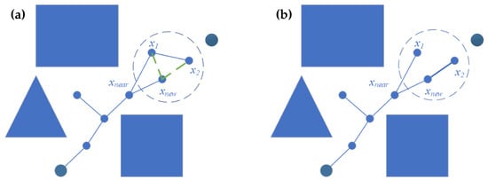
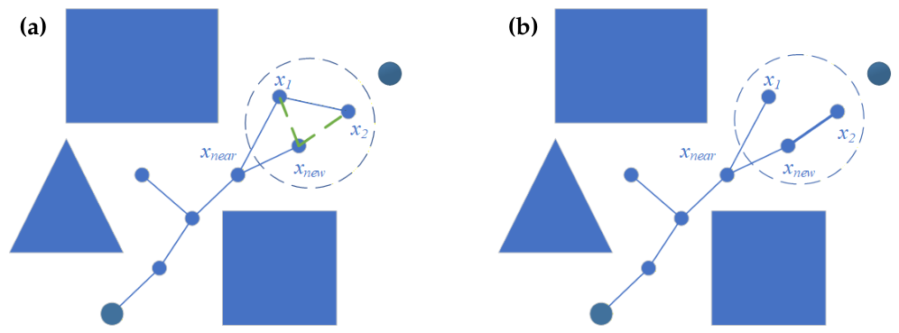
RRT* [18] augments each expansion of RRT with two cost-aware operations, so that path cost keeps decreasing as the tree grows. It retains the loop of Algorithm 1 but, after a collision-free extension, no longer attaches the new node ${\mathbf{x}}_{new}$ directly to the nearest node. Parent selection (Algorithm 2) instead inspects the nodes within a radius r of ${\mathbf{x}}_{new}$ and roots it at the collision-free neighbor that yields the lowest cost-to-come. Rewiring (Algorithm 3) then runs the same comparison in reverse: any nearby node that could reach the root more cheaply through ${\mathbf{x}}_{new}$ is re-parented to it. Figure 1 illustrates the two operations. Repeating these operations drives the tree toward the minimum-cost connection and, as sampling becomes dense, toward the globally optimal route.

Algorithm 1 RRT

Input:  ${\mathbf{x}}_{start}$, ${\mathbf{x}}_{goal}$, obstacle set O, step $\eta$, iteration cap $K_{max}$ Output:  a path from ${\mathbf{x}}_{start}$ to ${\mathbf{x}}_{goal}$, or ∅    1: $V\leftarrow \left\{{\mathbf{x}}_{start}\right\}$; $E\leftarrow \varnothing$    2: for $k=1$to $K_{max}$ do    3:     ${\mathbf{x}}_{rand}\leftarrow \mathit{Sample}\left({\mathcal{X}}_{free}\right)$    4:     ${\mathbf{x}}_{near}\leftarrow \mathit{Nearest}(V,{\mathbf{x}}_{rand})$    5:     ${\mathbf{x}}_{new}\leftarrow \mathit{Steer}({\mathbf{x}}_{near},{\mathbf{x}}_{rand},\eta )$    6:     if $\mathit{ObstacleFree}({\mathbf{x}}_{near},{\mathbf{x}}_{new},O)$ then    7:         $V\leftarrow V\cup \left\{{\mathbf{x}}_{new}\right\}$; $E\leftarrow E\cup \left\{({\mathbf{x}}_{near},{\mathbf{x}}_{new})\right\}$    8:         if $\mathit{Distance}({\mathbf{x}}_{new},{\mathbf{x}}_{goal})\le \eta$ and $\mathit{ObstacleFree}({\mathbf{x}}_{new},{\mathbf{x}}_{goal},O)$ then    9:            return $\mathit{ExtractPath}(V,E,{\mathbf{x}}_{new})$ with ${\mathbf{x}}_{goal}$ appended  10:         end if  11:     end if  12: end for  13: return ∅

Figure 1. Schematic of the RRT* extension. (a) ChooseParent selects, among the neighbors of ${\mathbf{x}}_{new}$ within the radius, the node connected to ${\mathbf{x}}_{new}$ by a collision-free edge that yields the lowest cost-to-come as its parent. (b) Rewire re-parents a nearby node to ${\mathbf{x}}_{new}$ when the connection through ${\mathbf{x}}_{new}$ lowers its cost. Blue polygons represent obstacles. The green dashed lines in (a) indicate candidate connections considered during parent selection. The larger dark-blue circles mark the start (lower left) and goal (upper right), while the smaller blue circles represent other tree nodes. Marker size distinguishes these roles and does not encode a numerical value.

Algorithm 2 ChooseParent

Input:  neighbor set $X_{near}$, nearest node ${\mathbf{x}}_{near}$, new node ${\mathbf{x}}_{new}$, obstacle set O Output:  parent node ${\mathbf{x}}_{par}$    1: ${\mathbf{x}}_{par}\leftarrow {\mathbf{x}}_{near}$    2: for each $v\in X_{near}$ do    3:     if $\mathit{ObstacleFree}(v,{\mathbf{x}}_{new},O)$ and $\mathit{Cost}\left(v\right)+\mathit{Distance}(v,{\mathbf{x}}_{new})<\mathit{Cost}\left({\mathbf{x}}_{par}\right)+\mathit{Distance}({\mathbf{x}}_{par},{\mathbf{x}}_{new})$ then    4:         ${\mathbf{x}}_{par}\leftarrow v$    5:     end if    6: end for    7: return ${\mathbf{x}}_{par}$

Algorithm 3 Rewire

Input:  tree $(V,E)$, neighbor set $X_{near}$, new node ${\mathbf{x}}_{new}$, obstacle set O Output:  updated tree $(V,E)$    1: for each $v\in X_{near}$ do    2:     if $\mathit{ObstacleFree}({\mathbf{x}}_{new},v,O)$ and $\mathit{Cost}\left({\mathbf{x}}_{new}\right)+\mathit{Distance}({\mathbf{x}}_{new},v)<\mathit{Cost}\left(v\right)$ then    3:         update the parent of v to ${\mathbf{x}}_{new}$    4:     end if    5: end for    6: return $(V,E)$

3.2. GB-RRT*

GB-RRT* introduces goal biasing into the sampling step. The preset probability $P_g$ takes the goal ${\mathbf{x}}_{goal}$ itself as the sample instead of a uniform draw, and it samples uniformly the rest of the time, while parent selection and rewiring remain as in RRT*. As shown in Algorithm 4, the goal-biased sampler replaces the sampling step of Algorithm 1. Sampling the goal at intervals directs the tree’s growth toward the target and reduces the effort spent on purely random exploration.

Algorithm 4 GoalBiasedSample

Input:  goal ${\mathbf{x}}_{goal}$, bias probability $P_g$ Output:  a sample ${\mathbf{x}}_{rand}$    1: if $\mathit{Rand}(0,1)<P_g$ then    2:     ${\mathbf{x}}_{rand}\leftarrow {\mathbf{x}}_{goal}$    3: else    4:     ${\mathbf{x}}_{rand}\leftarrow \mathit{Sample}\left({\mathcal{X}}_{free}\right)$    5: end if    6: return ${\mathbf{x}}_{rand}$

3.3. Informed-RRT*

Informed-RRT* [22] also acts on the sampler, taking effect once a first route is available. Until such a route exists, it samples the whole space, as in RRT*. Once a route of length $c_{best}$ is found, it restricts sampling to the prolate hyperspheroid whose foci are ${\mathbf{x}}_{start}$ and ${\mathbf{x}}_{goal}$ and whose transverse diameter is $c_{best}$, the set of points that can still shorten the route. Algorithm 5 draws a sample from this set by scaling, rotating, and translating a point of the unit ball. The point ${\mathbf{x}}_{ball}$ is drawn uniformly from the unit ball. The diagonal matrix $\mathbf{L}=\mathrm{diag}(r_1,r_2,\dots ,r_d)$ defines the hyperspheroid axes, where $r_1=c_{best}/2$ and $r_i=\sqrt{c_{best}^2-c_{min}^2}/2$ for $i=2,\dots ,d$. The rotation matrix $\mathbf{C}$ aligns the principal axis with the direction from ${\mathbf{x}}_{start}$ to ${\mathbf{x}}_{goal}$, and ${\mathbf{x}}_{center}=({\mathbf{x}}_{start}+{\mathbf{x}}_{goal})/2$ translates the hyperspheroid to the midpoint of the two foci. Thus, line 9 computes ${\mathbf{x}}_{rand}=\mathbf{C}\mathbf{L}{\mathbf{x}}_{ball}+{\mathbf{x}}_{center}$, which is a uniform sample in the informed set. The region contracts as $c_{best}$ decreases.

Algorithm 5 InformedSample

Input:  start ${\mathbf{x}}_{start}$, goal ${\mathbf{x}}_{goal}$, best path cost $c_{best}$ Output:  a sample ${\mathbf{x}}_{rand}$    1: if $c_{best}<\infty$then    2:     $c_{min}\leftarrow \mathit{Distance}({\mathbf{x}}_{start},{\mathbf{x}}_{goal})$    3:     ${\mathbf{x}}_{center}\leftarrow ({\mathbf{x}}_{start}+{\mathbf{x}}_{goal})/2$    4:     $\mathbf{C}\leftarrow \mathit{RotationToWorldFrame}({\mathbf{x}}_{start},{\mathbf{x}}_{goal})$    5:     $r_1\leftarrow c_{best}/2$    6:     $r_i\leftarrow \sqrt{c_{best}^2-c_{min}^2}/2$, for $i=2,\dots ,d$    7:     $\mathbf{L}\leftarrow \mathrm{diag}(r_1,r_2,\dots ,r_d)$    8:     ${\mathbf{x}}_{ball}\leftarrow \mathit{SampleUnitBall}\left(\right)$    9:     ${\mathbf{x}}_{rand}\leftarrow \mathbf{C}\mathbf{L}{\mathbf{x}}_{ball}+{\mathbf{x}}_{center}$  10: else  11:     ${\mathbf{x}}_{rand}\leftarrow \mathit{Sample}\left({\mathcal{X}}_{free}\right)$  12: end if  13: return ${\mathbf{x}}_{rand}$

3.4. Bi-RRT*

Bi-RRT* [29] accelerates the search structurally by running two trees at once, $T_{start}$ anchored at the start and $T_{goal}$ at the goal, and letting them advance in turn until they meet. On its turn, the active tree performs one RRT* growth step, inserting and locally re-optimizing ${\mathbf{x}}_{new}$ as above. In the original formulation, the new node is joined to the opposite tree through its neighbors inside a radius that shrinks as the trees grow, and the candidates are examined in ascending order of the cost of the resulting path. The baseline adopted here uses the simpler merge that is common in practice, in which the new node is matched to its nearest counterpart ${\mathbf{x}}_{connect}$ in the other tree, and the two branches are connected into a single start-to-goal path when the pair lies within a merge radius ${\eta }_c$, and no obstacle blocks the line joining them. Otherwise, the two trees swap roles for the next turn, and this alternation repeats until they connect or the sampling budget runs out. The full procedure is given in Algorithm 6, in which the growth primitive Extend carries out one RRT* growth step. Since neither tree has to span the whole start-to-goal distance but only reach the meeting point, the region each of them must explore is reduced.

Algorithm 6 Bi-RRT*

Input:  ${\mathbf{x}}_{start}$, ${\mathbf{x}}_{goal}$, obstacle set O, step $\eta$, radius r, merge radius ${\eta }_c$, iteration cap $K_{max}$ Output:  a path, or ∅    1: $T_a\leftarrow \left\{{\mathbf{x}}_{start}\right\}$; $T_b\leftarrow \left\{{\mathbf{x}}_{goal}\right\}$    2: for $k=1$ to $K_{max}$ do    3:     ${\mathbf{x}}_{new}\leftarrow \mathit{Extend}(T_a,O,\eta ,r)$    4:     if ${\mathbf{x}}_{new}\ne \varnothing$ then    5:         ${\mathbf{x}}_{connect}\leftarrow \mathit{Nearest}(T_b,{\mathbf{x}}_{new})$    6:         if $\mathit{Distance}({\mathbf{x}}_{new},{\mathbf{x}}_{connect})\le {\eta }_c$ and $\mathit{ObstacleFree}({\mathbf{x}}_{new},{\mathbf{x}}_{connect},O)$ then    7:            return $\mathit{Connect}(T_a,T_b,{\mathbf{x}}_{new},{\mathbf{x}}_{connect})$    8:         end if    9:     end if  10:     $\mathit{Swap}(T_a,T_b)$  11: end for  12: return ∅

4. The Proposed SACE-Bi-RRT* Algorithm

4.1. Overall Framework

This section presents SACE-Bi-RRT*, a bidirectional RRT* planner for three-dimensional static environments. Its design follows from two observations on existing bidirectional planners. First, in most of them, the connection module continually evaluates how far apart the two trees are and whether they can see each other, yet this information is not used in the extension decisions. Second, a colliding extension is discarded as a whole, although the collision exposes precisely the local geometry required to construct a detour. SACE-Bi-RRT* therefore lets the inter-tree gap and its visibility regulate the guided expansion, and turns the geometry exposed by a collision into a deterministic escape direction rather than discarding it.

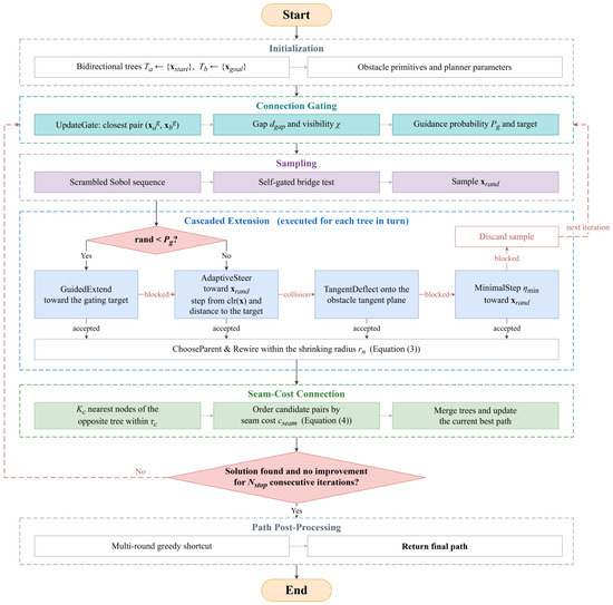
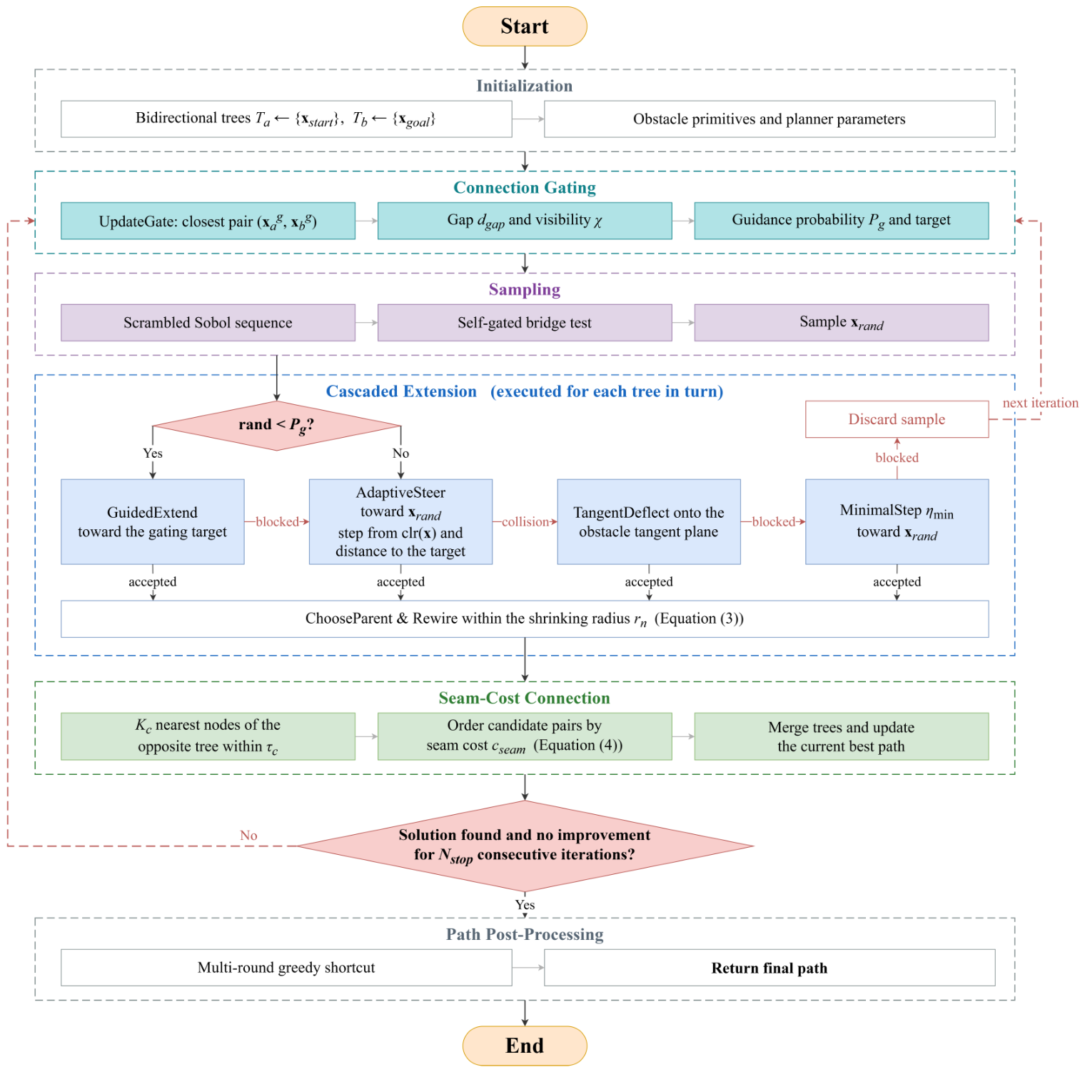
On this basis, the planner organizes its components into a connection-aware chain. An incremental query maintains the globally closest node pair between the two trees together with its line-of-sight visibility, and this information regulates the probability and the target of guided expansion toward the opposite tree (Section 4.2). When an extension collides, the direction toward the current guidance target is projected onto the tangent plane of the hit obstacle, which yields a deterministic sliding direction along the obstacle surface (Section 4.3). The extension step is adapted to the clearance of the expanding node and its distance to the extension target (Section 4.4). Global exploration is performed with scrambled Sobol sequences, reinforced by an in-obstacle-triggered bridge test for narrow passages (Section 4.5). Once the two trees are connected, the merged path is shortened by a multi-round greedy shortcut (Section 4.6). Figure 2 illustrates the overall workflow.

Figure 2. Overall workflow of SACE-Bi-RRT*. Colored blocks denote the components introduced in this work, and white blocks denote the operations inherited from Bi-RRT*. Solid arrows carry the forward flow, and dashed arrows return to the next iteration.

Both trees are grown as standard RRT* trees. An accepted node is connected to the minimum-cost parent among its neighbors within the shrinking radius.

$$r_n=min\left(\gamma {\left(\frac{logn}{n}\right)}^{1/3},{\eta }_{max}\right),$$

(3)

where n is the total number of nodes in the two trees, and $\gamma$ is the RRT* scaling constant. The bound ${\eta }_{max}$ is the upper limit of the extension step of Section 4.4. The neighbors are rewired through the new node whenever this lowers their cost.

After each insertion, the connection stage examines the $K_c$ nearest cross-tree neighbors of the newest node and keeps those within the connection tolerance ${\tau }_c$. The trees are merged at the first collision-free pair in ascending order of the seam cost:   

$$c_{seam}({\mathbf{x}}_i,{\mathbf{x}}_j)=g_a\left({\mathbf{x}}_i\right)+\parallel {\mathbf{x}}_i-{\mathbf{x}}_j\parallel +g_b\left({\mathbf{x}}_j\right),$$

(4)

where $g_a$ and $g_b$ are the cost-to-come functions of the start-rooted and goal-rooted trees, respectively. Specifically,

$$g_a\left({\mathbf{x}}_{start}\right)=0,g_b\left({\mathbf{x}}_{goal}\right)=0,g_q\left({\mathbf{x}}_{new}\right)=g_q\left({\mathbf{x}}_{par}\right)+\parallel {\mathbf{x}}_{new}-{\mathbf{x}}_{par}\parallel ,q\in \{a,b\}.$$

(5)

After parent selection and rewiring, $g_a\left({\mathbf{x}}_i\right)$ and $g_b\left({\mathbf{x}}_j\right)$ denote the current accumulated path lengths from the corresponding roots to these nodes. Since Equation (4) measures the cost of the complete path through the candidate pair rather than the pair distance alone, the connection favors pairs attached to low-cost branches in both trees over the geometrically closest pair.

The current best solution is replaced whenever a pair with a lower seam cost is found, and the search stops when a solution exists and no improvement has occurred for $N_{stop}$ consecutive iterations. Edge feasibility throughout the planner is verified by an exact segment-primitive intersection test on the parametric obstacles, whose closed-form clearance and normal queries are given in Section 4.3.

Algorithm 7 summarizes the main loop. Compared with Bi-RRT* (Algorithm 6), the modifications correspond to lines 4 and 5 (gating), line 7 (sampler), line 8 (guided expansion), lines 9 to 17 (cascaded extension), and line 22 (seam-cost connection in place of the nearest-pair merge). The following subsections describe each component in detail.

Algorithm 7 SACE-Bi-RRT*

Input:  ${\mathbf{x}}_{start}$, ${\mathbf{x}}_{goal}$, obstacle set O, iteration cap $K_{max}$, no-improvement bound $N_{stop}$ Output:  a collision-free path from ${\mathbf{x}}_{start}$ to ${\mathbf{x}}_{goal}$, or ∅    1: $T_a\leftarrow \left\{{\mathbf{x}}_{start}\right\}$; $T_b\leftarrow \left\{{\mathbf{x}}_{goal}\right\}$; initialize two scrambled Sobol streams    2: $(d_{gap},\chi )\leftarrow (\infty ,0)$    3: for $k=1$ to $K_{max}$ do    4:     $(d_{gap},\chi )\leftarrow \mathit{UpdateGate}(T_a,T_b)$    5:     $P_g\leftarrow \mathit{GatedProbability}(d_{gap},\chi )$; update the guidance target of each tree    6:     for each $T\in \{T_a,T_b\}$ do    7:         ${\mathbf{x}}_{sample}\leftarrow \mathit{SobolBridgeSample}\left(\mathcal{X}\right)$    8:         ${\mathbf{x}}_{new}\leftarrow \mathit{GuidedExtend}(T,P_g)$    9:         if ${\mathbf{x}}_{new}=\varnothing$ then  10:            ${\mathbf{x}}_{new}\leftarrow \mathit{AdaptiveSteer}(T,{\mathbf{x}}_{sample})$  11:            if the extension collided then  12:                ${\mathbf{x}}_{new}\leftarrow \mathit{TangentDeflect}(T,{\mathbf{x}}_{sample})$  13:            end if  14:            if ${\mathbf{x}}_{new}=\varnothing$ then  15:                ${\mathbf{x}}_{new}\leftarrow \mathit{MinimalStep}(T,{\mathbf{x}}_{sample})$  16:            end if  17:         end if  18:         if ${\mathbf{x}}_{new}\ne \varnothing$ then  19:            commit ${\mathbf{x}}_{new}$ to T by ChooseParent and Rewire within radius $r_n$  20:         end if  21:     end for  22:     $\mathit{TryConnect}(T_a,T_b)$  23:     if a solution exists and no improvement occurred for $N_{stop}$ iterations then  24:         break  25:     end if  26: end for  27: return the merged path after greedy shortcutting, or ∅ if no solution was found

4.2. Dual-Tree Guided Expansion Strategy

Goal biasing is a common method for accelerating RRT-type planners. In existing methods, however, the biasing probability is regulated by single-tree information only. It is either a constant probability, a probability decaying with the distance from one tree to the fixed goal, or an event-triggered switch driven by failure counts. In bidirectional search, the state that actually indicates whether a guided extension toward the opposite tree is beneficial, namely the gap between the two trees and the visibility across it, has not been coupled with the guidance decision. The dual-tree guided expansion strategy proposed here makes this coupling explicit: both the probability and the target of the guided extension are regulated by the inter-tree gap and its line-of-sight visibility.

Let $T_a,T_b\subset {\mathbb{R}}^3$ denote the node sets of the two trees. The gating pair is defined as the globally closest node pair between the two trees:

$$({\mathbf{x}}_a^g,{\mathbf{x}}_b^g)=\underset{{\mathbf{x}}_i\in T_a,{\mathbf{x}}_j\in T_b}{arg\; min}\parallel {\mathbf{x}}_i-{\mathbf{x}}_j\parallel ,d_{gap}=\parallel {\mathbf{x}}_a^g-{\mathbf{x}}_b^g\parallel .$$

(6)

Whether the two trees can see each other across this pair is described by the visibility flag

$$\chi =1\left[\overline{{\mathbf{x}}_a^g{\mathbf{x}}_b^g}\mathrm{is}\mathrm{collision}\text{-}\mathrm{free}\right]\in \{0,1\},$$

(7)

where $1[·]$ is the indicator function.

The pair is maintained incrementally. Every cross-tree pair created at iteration k involves a node inserted at that iteration, so comparing the newest node of each tree against all nodes of the opposite tree captures every new candidate. The record is updated only when a closer pair appears

$$d_{gap}^{\left(k\right)}=min\left(d_{gap}^{(k-1)},\underset{\mathbf{y}\in T_b}{min}\parallel {\mathbf{x}}_{new}^a-\mathbf{y}\parallel ,\underset{\mathbf{x}\in T_a}{min}\parallel \mathbf{x}-{\mathbf{x}}_{new}^b\parallel \right)\le d_{gap}^{(k-1)},$$

(8)

where ${\mathbf{x}}_{new}^a$ and ${\mathbf{x}}_{new}^b$ represent the nodes inserted at iteration k.

The update cost is of the same order as one nearest-neighbor query per tree. Equation (8) shows that $d_{gap}$ is non-increasing over the iterations, which makes it a stable regulating signal, and $\chi$ is re-evaluated only when the record pair is replaced, so each replacement incurs at most one additional collision check.

The gating pair regulates only the timing of the guided extension, whereas the trees are joined at the pair minimizing the seam cost of Equation (4) among the near neighbors of the newest nodes. That cost depends on the cost-to-come values, is not monotone, and changes under rewiring, which makes it unsuitable as a regulating signal.

A guided extension is most useful when the two trees are far apart and mutually visible. It brings no further benefit once the trees are already within the connection tolerance, where an aggressive bias only causes overshooting. It should be suppressed when the gating pair is occluded, since extending toward an invisible target repeatedly pushes the tree against the blocking obstacle. Accordingly, the guidance probability $P_g$ is defined first as

$$P_g=P_{min}+(P_{max}-P_{min})\chi S\left(z\right),$$

(9)

where $P_{min}$ and $P_{max}$ bound the probability from below and above, $\chi$ is the visibility flag of the gating pair, and $S\left(z\right)$ is a smoothstep function of the normalized gap z,

$$S\left(z\right)=3z^2-2z^3,z=clamp\left(\frac{d_{gap}-{\tau }_c}{d_h-{\tau }_c},0,1\right),$$

(10)

where ${\tau }_c$ denotes the connection tolerance and $d_h={\kappa }_h{\tau }_c$ with ${\kappa }_h>1$ the transition distance, so that z normalizes the gap over the transition band. The ceiling $P_{max}$ is kept moderate so that most iterations remain available for global sampling.

The polynomial $S\left(z\right)$ is the lowest-order polynomial satisfying $S\left(0\right)=0$, $S\left(1\right)=1$, and $S^{\prime }\left(0\right)=S^{\prime }\left(1\right)=0$. Compared with a linear map, it saturates smoothly at both ends of the transition band, so the sampling behavior does not switch abruptly when the gap crosses ${\tau }_c$ or $d_h$.

The guidance target follows the same visibility rule

$${\mathbf{x}}_{tgt}^{\left(a\right)}=\left\{\begin{array}{cc}{\mathbf{x}}_b^g,\hfill & \chi =1,\hfill \\ {\mathbf{x}}_g,\hfill & \chi =0,\hfill \end{array}\right.$$

(11)

and it is symmetrical for $T_b$, where ${\mathbf{x}}_g$ denotes the endpoint the tree grows toward.

With probability $P_g$, the tree performs a guided extension: it steers from its node closest to the guidance target toward that target, with the step clamped so as not to overshoot,

$${\mathbf{x}}_{new}={\mathbf{x}}_n^t+min\left(\eta \left({\mathbf{x}}_n^t\right),\parallel {\mathbf{x}}_{tgt}-{\mathbf{x}}_n^t\parallel \right){\displaystyle \frac{{\mathbf{x}}_{tgt}-{\mathbf{x}}_n^t}{\parallel {\mathbf{x}}_{tgt}-{\mathbf{x}}_n^t\parallel }},{\mathbf{x}}_n^t=\underset{\mathbf{x}\in T}{arg\; min}\parallel \mathbf{x}-{\mathbf{x}}_{tgt}\parallel ,$$

(12)

where $\eta (·)$ stands for the adaptive step.

If the guided extension is blocked, the iteration falls back to the sample-directed extension of the cascade in Algorithm 7, so no iteration is wasted. Four behaviors follow. When the two trees are far apart and mutually visible, $P_g$ approaches $P_{max}$, and the trees grow toward each other across the shrinking gap. When they are close and visible, $P_g$ falls to $P_{min}$, which avoids overshooting and leaves the merge to the connection stage. When the gating pair is occluded, the strategy degrades to a low-probability bias toward the tree’s endpoint, so that the tree does not repeatedly push against the blocking obstacle. The collisions that still occur are handled by the tangent-plane deflection. In all remaining iterations, the planner explores globally with the Sobol-based sampler. The complete procedure is summarized in Algorithm 8. In Algorithm 8, ${\mathbf{y}}_b$ and ${\mathbf{y}}_a$ are temporary nearest-node candidates used to update the record; the stored gating pair remains $({\mathbf{x}}_a^g,{\mathbf{x}}_b^g)$ throughout.

Algorithm 8 Gate update and guided extension

Input:  $T_a$, $T_b$, newest nodes ${\mathbf{x}}_{new}^a$ and ${\mathbf{x}}_{new}^b$, gate record $({\mathbf{x}}_a^g,{\mathbf{x}}_b^g,d_{gap},\chi )$, tree to extend T, obstacle set O Output:  a guided node ${\mathbf{x}}_{new}$ for tree T, or ∅    1: ${\mathbf{y}}_b\leftarrow \mathit{Nearest}(T_b,{\mathbf{x}}_{new}^a)$; ${\mathbf{y}}_a\leftarrow \mathit{Nearest}(T_a,{\mathbf{x}}_{new}^b)$    2: if $\mathit{Distance}({\mathbf{x}}_{new}^a,{\mathbf{y}}_b)<d_{gap}$ then    3:     $({\mathbf{x}}_a^g,{\mathbf{x}}_b^g)\leftarrow ({\mathbf{x}}_{new}^a,{\mathbf{y}}_b)$; $d_{gap}\leftarrow \mathit{Distance}({\mathbf{x}}_{new}^a,{\mathbf{y}}_b)$    4: end if    5: if $\mathit{Distance}({\mathbf{y}}_a,{\mathbf{x}}_{new}^b)<d_{gap}$ then    6:     $({\mathbf{x}}_a^g,{\mathbf{x}}_b^g)\leftarrow ({\mathbf{y}}_a,{\mathbf{x}}_{new}^b)$; $d_{gap}\leftarrow \mathit{Distance}({\mathbf{y}}_a,{\mathbf{x}}_{new}^b)$    7: end if    8: if the gating pair was replaced then $\chi \leftarrow \mathit{ObstacleFree}({\mathbf{x}}_a^g,{\mathbf{x}}_b^g,O)$    9: $z\leftarrow clamp\left((d_{gap}-{\tau }_c)/(d_h-{\tau }_c),0,1\right)$  10: $P_g\leftarrow P_{min}+(P_{max}-P_{min})·\chi ·(3z^2-2z^3)$  11: if $\chi =1$ then ${\mathbf{x}}_{tgt}\leftarrow$ the gating node of the tree opposite to T  12: else ${\mathbf{x}}_{tgt}\leftarrow$ the endpoint of T  13: if $\mathit{Rand}(0,1)\ge P_g$ then return ∅  14: ${\mathbf{x}}_n^t\leftarrow \mathit{Nearest}(T,{\mathbf{x}}_{tgt})$  15: ${\mathbf{x}}_{new}\leftarrow \mathit{Steer}({\mathbf{x}}_n^t,{\mathbf{x}}_{tgt},min(\eta \left({\mathbf{x}}_n^t\right),\mathit{Distance}({\mathbf{x}}_n^t,{\mathbf{x}}_{tgt})))$  16: if $\mathit{ObstacleFree}({\mathbf{x}}_n^t,{\mathbf{x}}_{new},O)$ then  17:     return ${\mathbf{x}}_{new}$  18: end if  19: return ∅

4.3. Tangent-Plane Deflection Strategy

The standard RRT* discards a sample whenever the extension toward it collides, although the collision itself reveals the local geometry of the blocking obstacle. Existing collision-exploiting strategies either deflect along one-dimensional obstacle boundaries in the plane, or, in three dimensions, draw K candidate directions inside a sampling cone that is unrelated to the goal direction, with K typically set to 8. To make direct use of the exposed geometry, a tangent-plane deflection strategy is proposed, in which the escape direction is derived from two explicit requirements. The direction should (i) leave the obstacle surface and, (ii) among all motions parallel to the surface, make the largest progress toward the current guidance target.

Since the obstacles are parametric primitives, namely spheres $[\mathbf{c},r]$, axis-aligned boxes $[\mathbf{c},\mathbf{h}]$ with half-extents $\mathbf{h}$, and z-axis cylinders $[\mathbf{c},r,H]$, the clearance of a query point $\mathbf{x}$ admits the closed form

$$\left\{\begin{array}{cc}\hfill \mathrm{clr}\left(\mathbf{x}\right)& =\underset{k}{min}{d}_k\left(\mathbf{x}\right),\hfill \\ \hfill d_k\left(\mathbf{x}\right)& =\left\{\begin{array}{cc}\parallel \mathbf{x}-{\mathbf{c}}_k\parallel -r_k,\hfill & \mathrm{sphere},\hfill \\ ∥max\left(|\mathbf{x}-{\mathbf{c}}_k|-{\mathbf{h}}_k,\mathbf{0}\right)∥,\hfill & \mathrm{box},\hfill \\ ∥\left[max\left(\parallel {\mathbf{x}}_{xy}-{\mathbf{c}}_{k,xy}\parallel -r_k,0\right),max\left(|x_z-c_{k,z}|-\frac{H_k}{2},0\right)\right]∥,\hfill & \mathrm{cylinder},\hfill \end{array}\right.\hfill \end{array}\right.$$

(13)

where $|·|$ and max are taken componentwise. The outward unit normal follows from the nearest surface point ${\mathbf{p}}^{*}$,

$$\hat{\mathbf{n}}\left(\mathbf{x}\right)={\displaystyle \frac{\mathbf{x}-{\mathbf{p}}^{*}}{\parallel \mathbf{x}-{\mathbf{p}}^{*}\parallel }},$$

(14)

evaluated analytically from the hit face, wall, or cap for a point lying on a surface.

When the extension from ${\mathbf{x}}_{near}$ collides, the last collision-free point ${\mathbf{x}}_{col}$ on the segment is located by bisection, and the outward unit normal $\hat{\mathbf{n}}$ of the hit obstacle at ${\mathbf{x}}_{col}$ is evaluated in closed form by Equation (14). Let ${\hat{\mathbf{u}}}_g=({\mathbf{x}}_{tgt}-{\mathbf{x}}_{col})/\parallel {\mathbf{x}}_{tgt}-{\mathbf{x}}_{col}\parallel$ denote the direction toward the guidance target of Equation (11). Requirement (ii) then takes the form of the constrained problem

$${\mathbf{t}}^{*}=\underset{\parallel \mathbf{t}\parallel =1,\mathbf{t}·\hat{\mathbf{n}}=0}{arg\; max}\left(\mathbf{t}·{\hat{\mathbf{u}}}_g\right).$$

(15)

The goal direction is decomposed into its normal and tangential components as follows:

$${\hat{\mathbf{u}}}_g=({\hat{\mathbf{u}}}_g·\hat{\mathbf{n}})\hat{\mathbf{n}}+{\mathbf{u}}_t,{\mathbf{u}}_t\perp \hat{\mathbf{n}}.$$

(16)

For every feasible $\mathbf{t}$, the Cauchy–Schwarz inequality gives

$$\mathbf{t}·{\hat{\mathbf{u}}}_g=\mathbf{t}·{\mathbf{u}}_t\le \parallel \mathbf{t}\parallel \parallel {\mathbf{u}}_t\parallel =\parallel {\mathbf{u}}_t\parallel ,$$

(17)

with equality if and only if $\mathbf{t}$ is aligned with ${\mathbf{u}}_t$. The solution of Equation (15) is therefore the normalized tangential projection of the goal direction

$${\mathbf{t}}^{*}={\displaystyle \frac{{\hat{\mathbf{u}}}_g-({\hat{\mathbf{u}}}_g·\hat{\mathbf{n}})\hat{\mathbf{n}}}{\parallel {\hat{\mathbf{u}}}_g-({\hat{\mathbf{u}}}_g·\hat{\mathbf{n}})\hat{\mathbf{n}}\parallel }},$$

(18)

which is well defined unless ${\hat{\mathbf{u}}}_g$ is parallel to $\hat{\mathbf{n}}$. In that degenerate case, an arbitrary tangential unit vector is used instead. Requirement (i) is met by mixing a fixed normal component into the sliding direction

$${\mathbf{d}}^{*}={\displaystyle \frac{{\lambda }_n\hat{\mathbf{n}}+{\lambda }_t{\mathbf{t}}^{*}}{\parallel {\lambda }_n\hat{\mathbf{n}}+{\lambda }_t{\mathbf{t}}^{*}\parallel }},{\lambda }_n,{\lambda }_t>0,$$

(19)

where ${\lambda }_n$ and ${\lambda }_t$ weight the surface-leaving and the goal-sliding components. Since ${\mathbf{t}}^{*}\perp \hat{\mathbf{n}}$, the denominator of Equation (19) equals $\sqrt{{\lambda }_n^2+{\lambda }_t^2}$, and the normal component of the escape direction is

$${\mathbf{d}}^{*}·\hat{\mathbf{n}}={\displaystyle \frac{{\lambda }_n}{\sqrt{{\lambda }_n^2+{\lambda }_t^2}}}>0,$$

(20)

so every escape direction points away from the surface.

A single direction may still be blocked in concave regions, where several obstacles jointly bound the free space around the collision point. Because $\{{\mathbf{t}}^{*},\hat{\mathbf{n}}\times {\mathbf{t}}^{*}\}$ is an orthonormal basis of the tangent plane, rotating ${\mathbf{t}}^{*}$ within the plane,

$${\mathbf{t}}_{\theta }=cos\theta {\mathbf{t}}^{*}+sin\theta (\hat{\mathbf{n}}\times {\mathbf{t}}^{*}),\theta \in \{0^{\circ },\pm {40}^{\circ },\pm {80}^{\circ }\},$$

(21)

yields a deterministic fan of five tangential candidates centered on the optimum of Equation (15). Substituting each candidate ${\mathbf{t}}_{\theta }$ into Equation (19) yields the escape direction ${\mathbf{d}}_{\theta }$. Each direction is extended from the collision point with the clearance-controlled saturated step

$${\eta }_{col}=max\left(min\left({\eta }_b\frac{\mathrm{clr}\left({\mathbf{x}}_{col}\right)}{d_{safe}},{\eta }_{max}\right),{\eta }_{min}\right).$$

(22)

This is the clearance factor of Section 4.4, kept above the same lower bound and without the target-approaching factor, because the purpose of the deflection is to leave the surface rather than to approach the target. Every candidate node ${\mathbf{x}}_{cand}={\mathbf{x}}_{col}+{\eta }_{col}{\mathbf{d}}_{\theta }$ is tested by the exact segment collision check from ${\mathbf{x}}_{near}$. Among the feasible candidates, the one minimizing

$$C=w_d\parallel {\mathbf{x}}_{near}-{\mathbf{x}}_{cand}\parallel +w_g\parallel {\mathbf{x}}_{cand}-{\mathbf{x}}_{tgt}\parallel +w_s{\displaystyle \frac{d_{safe}}{\mathrm{clr}\left({\mathbf{x}}_{cand}\right)+ϵ}}$$

(23)

is accepted, where the three terms penalize the extension length, the remaining distance to the guidance target, and the inverse clearance of the candidate node, respectively. The corresponding weights are $w_d$, $w_g$, and $w_s$.

The complete deflection procedure is summarized as follows.

Step 1. Locate the last collision-free point ${\mathbf{x}}_{col}$ on the blocked segment by bisection, and evaluate the outward unit normal $\hat{\mathbf{n}}$ of the hit obstacle at ${\mathbf{x}}_{col}$ by Equation (14).

Step 2. Project the direction ${\hat{\mathbf{u}}}_g$ toward the current guidance target onto the tangent plane and normalize it to obtain ${\mathbf{t}}^{*}$ by Equation (18). If ${\hat{\mathbf{u}}}_g$ is parallel to $\hat{\mathbf{n}}$, take an arbitrary tangential unit vector instead.

Step 3. Rotate ${\mathbf{t}}^{*}$ within the tangent plane by Equation (21) to generate the five tangential candidates, and mix the fixed normal component into each of them by Equation (19).

Step 4. Extend each candidate direction from ${\mathbf{x}}_{col}$ with the saturated step ${\eta }_{col}$ of Equation (22), and test every candidate node by the exact segment collision check from ${\mathbf{x}}_{near}$.

Step 5. Among the feasible candidates, accept the one minimizing the cost of Equation (23). If no candidate is feasible, report failure, and the cascade of Algorithm 7 falls back to the minimal-step extension toward the sample.

4.4. Adaptive Step Size

The free-space scale around an expanding node varies across the workspace by orders of magnitude, from narrow passages to open regions, yet the extension step of standard RRT* is one global constant. A constant step is thus mismatched with most of the workspace: it is too aggressive near obstacle surfaces and too conservative in open space. Adaptive step-size schemes have therefore been adopted in several RRT* variants. In the proposed planner, the step is required to scale with the clearance of the expanding node, so that the tree advances with small steps near obstacle surfaces and with large steps in free space. The step is further required to shrink as the node approaches the extension target, so that the extension does not overshoot. Both requirements are expressed as saturated factors of the clearance and of the target distance

$$\left\{\begin{array}{cc}\hfill f_{clr}& =min\left({\eta }_b\frac{\mathrm{clr}\left({\mathbf{x}}_{near}\right)}{d_{safe}},{\eta }_{max}\right),\hfill \\ \hfill f_{tgt}& =min\left(1,\frac{\parallel {\mathbf{x}}_{near}-{\mathbf{x}}_{tgt}\parallel }{{\eta }_{max}}\right),\hfill \end{array}\right.$$

(24)

where ${\eta }_b$ denotes the nominal step, $d_{safe}$ the reference clearance, and ${\mathbf{x}}_{tgt}$ the target of the current extension. For a guided extension, this target is the guidance target; otherwise, it is the sample point.

The step is their product, kept above a lower bound:

$$\eta =max\left(f_{clr}·f_{tgt},{\eta }_{min}\right).$$

(25)

Equation (25) confines $\eta$ to $[{\eta }_{min},{\eta }_{max}]$ and makes it non-decreasing both in the clearance and in the distance to the target. The two saturations give the step an explicit limiting behavior:

$$\eta =\left\{\begin{array}{cc}{\eta }_{min},\hfill & \mathrm{clr}\left({\mathbf{x}}_{near}\right)\le \frac{{\eta }_{min}}{{\eta }_b}{d}_{safe},\hfill \\ {\eta }_{max},\hfill & \mathrm{clr}\left({\mathbf{x}}_{near}\right)\ge \frac{{\eta }_{max}}{{\eta }_b}{d}_{safe}\wedge \parallel {\mathbf{x}}_{near}-{\mathbf{x}}_{tgt}\parallel \ge {\eta }_{max}.\hfill \end{array}\right.$$

(26)

That is, the step stays at the lower-bound value in the immediate vicinity of obstacle surfaces, reaches the full value in open space far from the target, and it varies linearly with the clearance between the two regimes. The step is applied in the steer operation toward the sample,

$${\mathbf{x}}_{new}={\mathbf{x}}_{near}+min\left(\eta ,\parallel {\mathbf{x}}_{sample}-{\mathbf{x}}_{near}\parallel \right){\displaystyle \frac{{\mathbf{x}}_{sample}-{\mathbf{x}}_{near}}{\parallel {\mathbf{x}}_{sample}-{\mathbf{x}}_{near}\parallel }},$$

(27)

where the inner minimum prevents the extension from overshooting the sample itself.

The guided extension applies the same rule toward the guidance target in Equation (12), and the tangent-plane deflection uses only the clearance factor in its saturated form in Equation (22). All four step parameters are tied to a single environment scale, the length L of the workspace diagonal, through the base step ${\eta }_b=L/40$. The remaining three are fixed multiples of this base step

$$d_{safe}=3{\eta }_b,{\eta }_{max}=\frac{8}{3}{\eta }_b,{\eta }_{min}=0.2{\eta }_b,$$

(28)

so the mapping transfers across environments of different sizes without retuning.

Very close to a surface, the lower bound ${\eta }_{min}$ may exceed the local clearance, so Equations (24)–(26) alone do not guarantee a collision-free extension. The feasibility of every candidate node and edge is enforced by the exact collision check, and the lower bound only prevents the step from vanishing.

4.5. Sobol-Sequence-Based Sampling Strategy

Pseudo-random sampling suffers from clusters and voids: some regions receive redundant samples while others remain uncovered for many iterations. These deficiencies directly lead to repeated exploration of covered regions and delayed discovery of uncovered ones, and low-discrepancy sequences have therefore been adopted in several planners to improve the coverage uniformity. Uniform coverage alone, however, rarely places samples inside narrow passages. The sampler of SACE-Bi-RRT* therefore combines two parts: a scrambled Sobol basis for global exploration, and a bridge test triggered by in-obstacle samples, which converts them into narrow-passage samples.

The Sobol sequence is a digital sequence in base 2. For coordinate j, a set of direction numbers $v_1^{\left(j\right)},v_2^{\left(j\right)},\dots \in [0,1)$ is generated from a primitive polynomial over $GF\left(2\right)$ assigned to that coordinate. The n-th sample is then assembled by XOR-combining the direction numbers selected by the binary digits of the index

$$n=\sum _{k\ge 1}{b}_k\left(n\right)2^{k-1},u_n^{\left(j\right)}=b_1\left(n\right)v_1^{\left(j\right)}\oplus b_2\left(n\right)v_2^{\left(j\right)}\oplus \cdots ,$$

(29)

where $b_k\left(n\right)\in \{0,1\}$ are the binary digits of n, and ⊕ denotes bitwise exclusive-or on the binary expansions.

To decorrelate the two trees without losing the low-discrepancy structure, each tree randomizes its own copy of the sequence by Owen–Matoušek scrambling. The scrambling applies a random nonsingular lower-triangular matrix ${\mathbf{C}}^{\left(j\right)}$ and a random digital shift ${\mathbf{e}}^{\left(j\right)}$ to the digit vector of every coordinate,

$${\tilde{\mathbf{u}}}^{\left(j\right)}={\mathbf{C}}^{\left(j\right)}{\mathbf{u}}^{\left(j\right)}\oplus {\mathbf{e}}^{\left(j\right)}\mathrm{over}GF\left(2\right).$$

(30)

A different scrambling seed is used per tree, so the two trees explore with two separately randomized low-discrepancy streams instead of tracing the same deterministic point set. The scrambled point ${\tilde{\mathbf{u}}}_n\in {[0,1]}^3$ is finally mapped affinely into the workspace

$${\mathbf{x}}_1={\mathbf{x}}_{lo}+{\tilde{\mathbf{u}}}_n\odot ({\mathbf{x}}_{hi}-{\mathbf{x}}_{lo}),$$

(31)

where ${\mathbf{x}}_{lo}$ and ${\mathbf{x}}_{hi}$ are the corners of the workspace, and ⊙ denotes the componentwise product.

The coverage uniformity of a point set $P=\{{\mathbf{u}}_1,\dots ,{\mathbf{u}}_N\}$ is assessed by two standard measures. The star discrepancy, which is highly sensitive to the point distribution near the corners and boundaries of the domain, is defined as

$$D_N^{*}\left(P\right)=\underset{\mathbf{t}\in {[0,1]}^d}{sup}\left|{\displaystyle \frac{1}{N}}{\displaystyle \sum _{i=1}^N}{1}_{[\mathbf{0},\mathbf{t})}\left({\mathbf{u}}_i\right)-t_1{t}_2\cdots t_d\right|.$$

(32)

The L2-star discrepancy replaces the supremum with an average over all anchored boxes

$$D_{L2}\left(P\right)={\left({\int }_{{[0,1]}^d}|{\displaystyle \frac{1}{N}}{\displaystyle \sum _{i=1}^N}{1}_{[\mathbf{0},\mathbf{t})}\left({\mathbf{u}}_i\right)-t_1{t}_2\cdots t_d{|}^2\mathrm{d}\mathbf{t}\right)}^{1/2},$$

(33)

where $[\mathbf{0},\mathbf{t})$ stands for the axis-aligned box anchored at the origin with upper corner $\mathbf{t}$, whose volume equals $t_1{t}_2\cdots t_d$.

Sobol sequences attain the low-discrepancy rate in dimension $d=3$,

$$\left\{\begin{array}{cc}\hfill D_N^{*}\left(\mathrm{Sobol}\right)& =O\left(\frac{{(logN)}^3}{N}\right),\hfill \\ \hfill D_N^{*}\left(\mathrm{random}\right)& =O\left(N^{-1/2}\right)\mathrm{in}\mathrm{probability},\hfill \end{array}\right.$$

(34)

so the deviation of the sampled set from the uniform measure shrinks at a nearly $N^{-1}$ rate, compared with the $N^{-1/2}$ rate of independent uniform points. Scrambling preserves this rate while randomizing the stream.

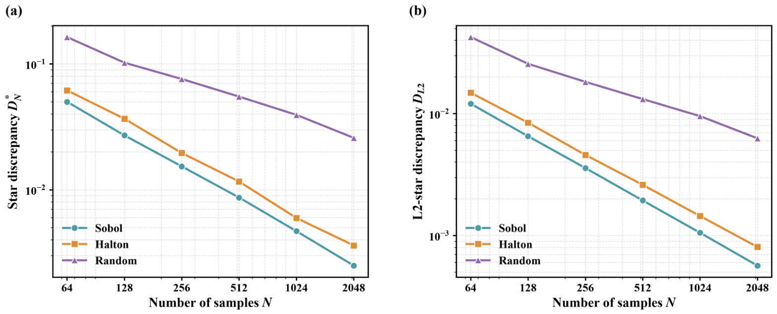
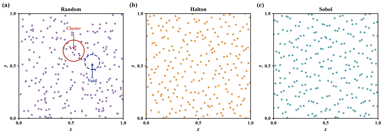
Figure 3 compares both measures of the employed scrambled Sobol points against Halton and pseudo-random points over the sample counts used by the planner, and the scrambled Sobol set attains the lowest discrepancy under both measures throughout. Figure 4 shows the corresponding point-distribution cross-sections, where the Sobol and Halton sets exhibit neither the clusters nor the voids that mark the pseudo-random set.

Figure 3. Discrepancy of the sampling sequences in dimension $d=3$ against the number of samples N. (a) Star discrepancy $D_N^{*}$. (b) L2-star discrepancy $D_{L2}$. Both axes are logarithmic.

Figure 4. Point-distribution cross-sections of the three sequences over a central slab of an $N=2048$ set. (a) Pseudo-random points, with a representative cluster and void marked. (b) Halton points. (c) Scrambled Sobol points.

The bridge test is triggered only when the Sobol sample ${\mathbf{x}}_1$ falls inside an obstacle, i.e., $\mathrm{clr}\left({\mathbf{x}}_1\right)\le 0$. A second point is then drawn along a random unit direction $\hat{\mathbf{v}}$ at the obstacle-gap scale,

$${\mathbf{x}}_2={\mathbf{x}}_1+{\ell }_b\hat{\mathbf{v}},{\ell }_b={\sigma }_b(0.5+1.5u),u\sim U(0,1),$$

(35)

where ${\sigma }_b$ is the bridge length scale, and ${\ell }_b$ is the sampled bridge-segment length. The midpoint ${\mathbf{x}}_m=({\mathbf{x}}_1+{\mathbf{x}}_2)/2$ is accepted if both endpoints lie inside obstacles while the midpoint keeps a clearance margin

$$\mathrm{clr}\left({\mathbf{x}}_1\right)\le 0\wedge \mathrm{clr}\left({\mathbf{x}}_2\right)\le 0\wedge \mathrm{clr}\left({\mathbf{x}}_m\right)\ge R_{safe},$$

(36)

where $R_{safe}$ denotes the required safety-clearance threshold at the bridge midpoint, specified in meters because it is a platform-level safety margin rather than a workspace-scale planning parameter, and ${\mathbf{x}}_2$ and ${\mathbf{x}}_m$ are additionally required to lie within the workspace.

Condition (36) constrains the accepted sample to a narrow passage bounded on both sides. The clearance margin guarantees a collision-free ball of radius $R_{safe}$ around ${\mathbf{x}}_m$, while the free chord through ${\mathbf{x}}_m$ along the bridge direction is contained between the two in-obstacle endpoints. Let $w\left({\mathbf{x}}_m\right)$ denote the extent of free space through ${\mathbf{x}}_m$ along $\hat{\mathbf{v}}$. The local passage width is then bounded on both sides,

$$2R_{safe}\le w\left({\mathbf{x}}_m\right)\le {\ell }_b\le 2{\sigma }_b,$$

(37)

which is exactly the narrow-passage regime that uniform sampling rarely reaches: open regions violate the upper bound, and gaps too tight for the planner violate the lower bound. The complete sampler returns

$${\mathbf{x}}_{sample}=\left\{\begin{array}{cc}{\mathbf{x}}_1,\hfill & \mathrm{clr}\left({\mathbf{x}}_1\right)>0,\hfill \\ {\mathbf{x}}_m,\hfill & \mathrm{condition}\left(36\right)\mathrm{holds},\hfill \\ {\mathbf{x}}_1^{\prime },\hfill & \mathrm{otherwise},\hfill \end{array}\right.$$

(38)

where ${\mathbf{x}}_1^{\prime }$ is a fresh Sobol point drawn by Equations (29)–(31).

As in standard uniform sampling, the fallback sample may still lie inside an obstacle. Feasibility is enforced by the subsequent steering and collision checks of Algorithm 7.

The in-obstacle trigger requires one clearance query per sample, and the bridge is rarely triggered in open regions, so the overhead remains small. The triggered bridge consumes only samples that would otherwise be discarded.

4.6. Path Post-Processing

The merged path inherits the zigzag redundancy typical of sampling-based planners, especially near the junction where the two trees join. The final path is therefore shortened by a multi-round greedy shortcut. Let $\mathrm{\Pi }=({\pi }_1,\dots ,{\pi }_N)$ denote the waypoint list. In each round, the procedure walks along the path once: from the current waypoint ${\pi }_i$, it connects directly to the farthest waypoint reachable by a collision-free straight segment,

$$j^{*}=max\left\{j>i+1:\overline{{\pi }_i{\pi }_j}\mathrm{is}\mathrm{collision}\text{-}\mathrm{free}\right\},$$

(39)

removes the intermediate waypoints ${\pi }_{i+1},\dots ,{\pi }_{j^{*}-1}$, and continues from ${\pi }_{j^{*}}$. If no such $j^{*}$ exists, it advances to ${\pi }_{i+1}$. At most three rounds are executed, and the procedure terminates early once a round removes no waypoint. Every replacement obeys the triangle inequality,

$$\parallel {\pi }_i-{\pi }_{j^{*}}\parallel \le {\displaystyle \sum _{k=i}^{j^{*}-1}}\parallel {\pi }_k-{\pi }_{k+1}\parallel ,$$

(40)

so the path length is monotonically non-increasing, and since every inserted segment passes the exact collision check, feasibility is preserved.

The cost of the shortcut, $O\left(N^2\right)$ collision checks per round on the sparse waypoint list, is negligible compared with that of the main loop.

5. Simulation Experiments and Analysis

This section evaluates SACE-Bi-RRT* by simulation. The contribution of the proposed components is isolated first; the full planner is then benchmarked against five baseline planners in two structured environments and in a large-scale mixed environment, and the mechanisms behind the observed results are examined at the end of the section. The baselines are RRT*, goal-biased RRT* (GB-RRT*), Informed-RRT*, Bi-RRT* and the artificial-potential-field guided bidirectional planner Bi-APF-RRT*. All planners are implemented in the same MATLAB framework and share the collision checking, the nearest-neighbor routine, the pre-allocated tree structure and the same anytime stopping rule, so each baseline also keeps optimizing after its first solution and terminates only after $N_{stop}$ iterations without improvement. Every run is executed in MATLAB R2025a on a computer equipped with an Intel Core i7-13700H processor and 16 GB of RAM.

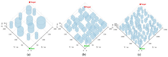
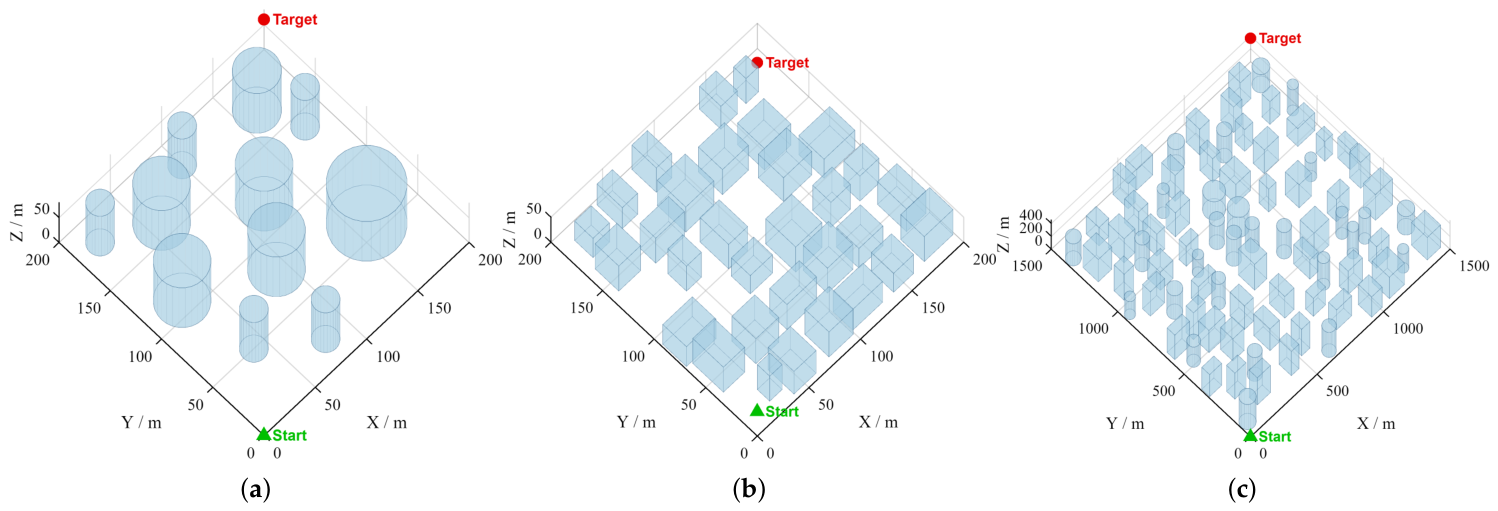
Three simulation environments were designed and are shown together in Figure 5. Environment 1 is a pillar forest of 200 m × 200 m × 80 m in which 11 full-height cylinders are placed in a staggered layout. A large-radius cylinder blocks the direct corridor near the diagonal, and another cylinder guards the goal region. The start and the goal are located at (0, 0, 0) and (200, 200, 60). The corridors of this scene are wide and few, so the result depends on how early a planner commits to one of them and on how it clears the obstacle at the end of the route. Environment 2 is a low-altitude urban block of 200 m × 200 m × 50 m in which 31 cuboid buildings are arranged on a jittered grid, and the gap between two neighboring buildings ranges from about 1 m to 13 m. Half of the buildings reach the ceiling of the workspace to prevent trivial flight over the scene, and the route runs from (10, 10, 10) to (190, 190, 10). The free space here is a street network whose direction changes are imposed by the intersections, which tests the ability of a planner to select streets without spending search time on the wrong ones. Environment 3 contains 80 obstacles, namely 52 cuboids and 28 cylinders, distributed over a 1500 m × 1500 m × 450 m workspace, and the start (0, 0, 0) and the goal (1490, 1490, 400) lie about 2.1 km apart along a straight line. Its search space is an order of magnitude larger than that of the two structured scenes. With a fixed sampling budget, the workspace receives fewer samples per unit volume, so the planner must maintain its behavior even though each detour spans a longer distance.

Figure 5. Three simulation environments. (a) Pillar forest. (b) Urban block. (c) Large-scale mixed environment.

All length-related parameters of SACE-Bi-RRT* are normalized by the diagonal length L of the workspace, so a single parameter set serves the three environments without per-scene tuning. The search stops after $N_{stop}=300$ iterations without improvement, and every run is capped at 5000 iterations. For the single-tree baselines, the goal-biasing probability is set to 0.1, and the extension step is fixed at ${\eta }_b$, and Informed-RRT* switches to ellipsoidal informed sampling once a first solution is available. Bi-RRT* grows two trees from the endpoints with the fixed step and merges them at the nearest node pair, and Bi-APF-RRT* additionally steers each extension by an artificial-potential-field resultant of goal attraction and obstacle repulsion. Neither bidirectional baseline applies post-processing. The complete values of the parameters of SACE-Bi-RRT*, together with the meaning of every symbol, are listed in Table A1 of Appendix A.

Each algorithm is run 100 times independently in every environment with the random seeds fixed to the run index. Two groups of indicators are recorded. The first group characterizes the first solution and consists of the first-solution time and the success rate within the iteration cap. The second group characterizes the converged result and consists of the final path length, the average turning angle, the number of iterations and the converged planning time. The average turning angle is the mean angle between consecutive segments of the returned path and quantifies its geometric smoothness, which the path length does not capture. All indicators are reported as the mean and the standard deviation over the 100 runs, except the number of iterations, which is reported as the mean. The success rate is 100% for every algorithm in every environment, so only the remaining indicators are tabulated.

5.1. Component Validation

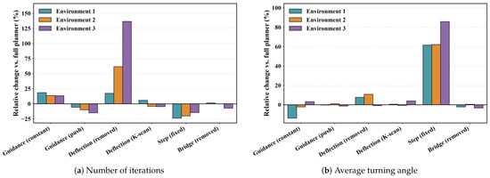
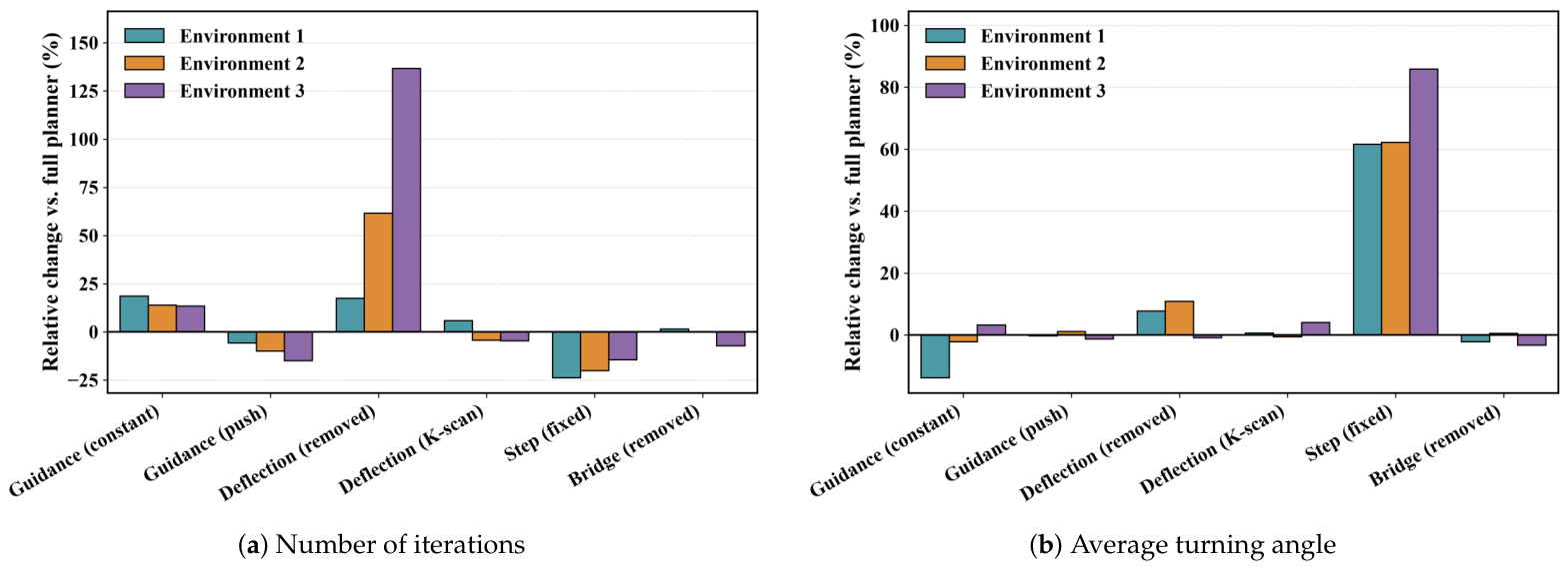
The proposed components act at successive stages of one extension, and each of them is examined separately before the full comparisons. Six variants are derived from the full planner, namely removing the bridge test from the sampler, replacing the gated guidance probability with the constant 0.1, replacing the visibility gate with a push-mode gate that keeps pursuing the opposite tree when the gap is blocked, removing the tangent-plane deflection, replacing the closed-form deflection direction with the K-direction scan, and removing the adaptive step. Each variant is run 30 times in every environment with the same fixed seeds. Table 1 reports the change in each affected metric relative to the full planner, and Figure 6 visualizes the changes in the number of iterations and in the average turning angle. Each variant modifies a single component, so the reported changes are marginal effects and are not additive, and each mean is taken over the successful runs of the variant.

Table 1. Ablation of the proposed components (a positive value denotes degradation). Each cell lists the change in Environment 1, in Environment 2 and in Environment 3.

Variant	Path Length (%)	Iterations (%)	Turning Angle (%)	Time (%)
Bridge (removed)	$+0.3$/$-0.2$/$-0.2$	$+1.6$/$-0.1$/$-7.2$	$-2.2$/$+0.5$/$-3.3$	$+8.5$/$-4.8$/$-16.2$
Guidance (constant)	$-0.9$/$-0.1$/$-0.3$	$+18.6$/$+14.0$/$+13.4$	$-13.8$/$-2.2$/$+3.2$	$+7.1$/$+4.8$/$+11.4$
Guidance (push)	$+0.6$/$-0.1$/$-0.3$	$-5.8$/$-9.9$/$-14.9$	$-0.3$/$+1.2$/$-1.3$	$+3.1$/$-13.3$/$-18.0$
Deflection (removed)	$+0.4$/$+3.3$/$+0.4$	$+17.5$/$+61.7$/$+136.6$	$+7.8$/$+10.8$/$-0.8$	$-12.2$/$+3.2$/$+67.9$
Deflection (K-scan)	$+0.3$/$+0.1$/$+0.2$	$+5.8$/$-4.3$/$-4.6$	$+0.7$/$-0.6$/$+4.0$	$-3.2$/$+4.6$/$+12.9$
Step (fixed)	$+2.6$/$+13.3$/$+9.8$	$-23.8$/$-20.1$/$-14.4$	$+61.6$/$+62.2$/$+85.9$	$-38.6$/$-35.0$/$+721.9$

Figure 6. Ablation results in the three environments. (a) Relative change in the number of iterations. (b) Relative change in the average turning angle.

The bridge test does not improve path quality in the three tested environments. None of the environments contains a passage that satisfies both bounds of Equation (37), so the test rarely yields an accepted sample, and removing it changes the path length by at most 0.3%, which remains within the run-to-run variation. Its timing effect is environment-dependent: removing it changes the planning time by $+8.5\%$, $-4.8\%$, and $-16.2\%$ in the three environments, respectively, with the reduction in the large-scale mixed environment being statistically significant. The bridge test is therefore retained as a safeguard for narrow passages that satisfy the bounds of Equation (37), rather than as a component responsible for the path-quality improvement.

The gated guidance mainly affects search effort rather than final path quality. Replacing it with a constant probability increases the number of iterations by 13.4–18.6% and the planning time by 4.8–11.4%, while changing the path length by less than 0.9%. The gate therefore improves the efficiency of the search without materially changing the final path quality.

The tangent-plane deflection is the component most critical to search robustness. Removing it increases the number of iterations by 17.5%, 61.7%, and 136.6% in the three environments, and reduces the success rate from 100% to 96.7% in the large-scale mixed environment. By contrast, replacing the closed-form direction with the K-direction scan produces no measurable path-quality gain: the two variants differ in path length by at most 0.3%, whereas the scan evaluates eight candidate directions instead of five and changes the planning time by $-3.2\%$, $+4.6\%$, and $+12.9\%$. The closed-form direction is therefore retained as the default.

The adaptive step primarily contributes to path quality. Replacing it with a fixed step reduces the number of iterations by 14.4–23.8% and shortens the planning time in the two structured environments by approximately 35–39%, but increases the final path length by 2.6–13.3% and the average turning angle by 61.6–85.9%. This result shows that the adaptive step trades additional search effort for shorter and smoother paths.

5.2. Structured Environments

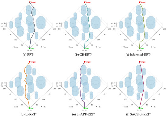
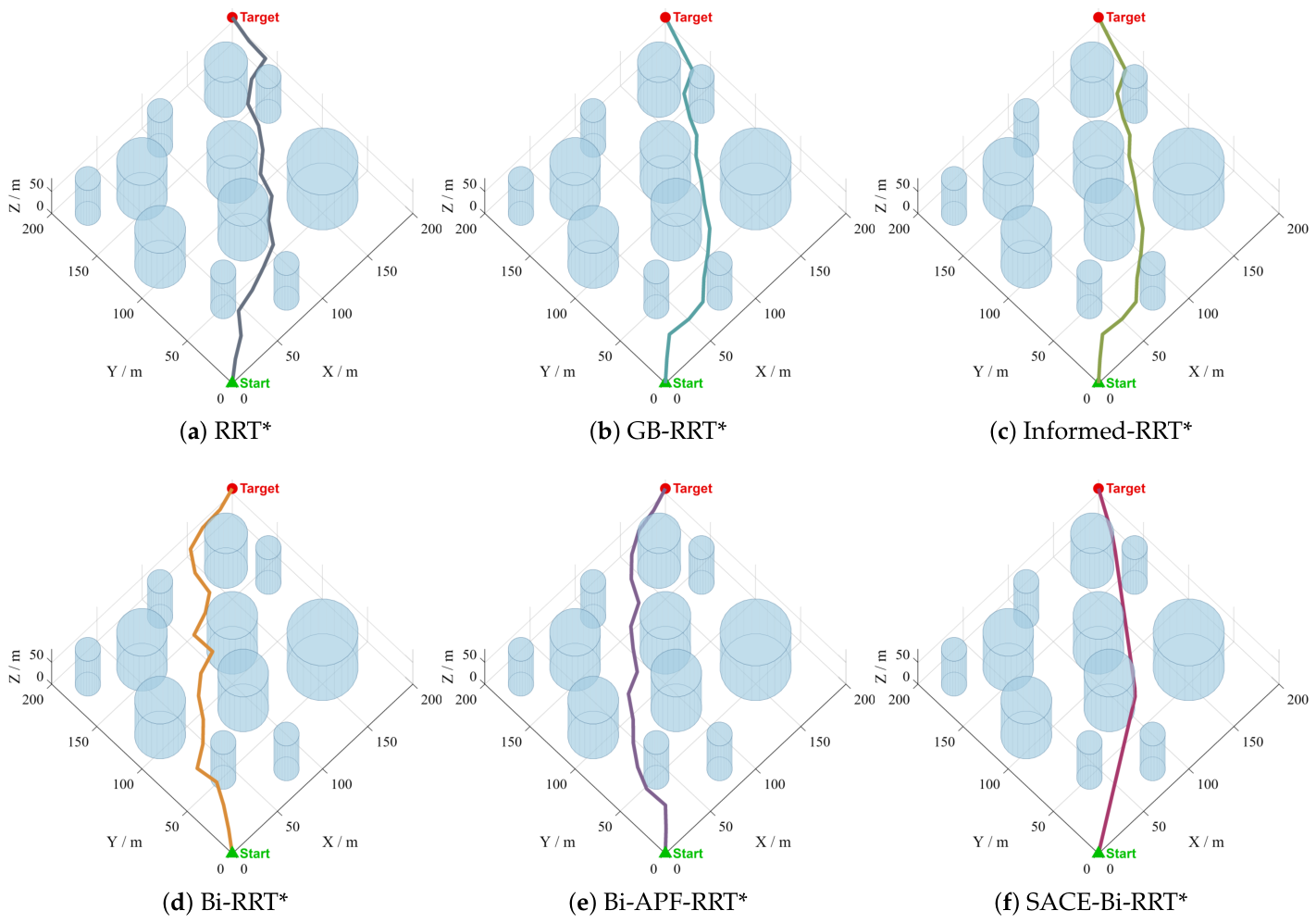
Figure 7 shows the planning results in the pillar forest. RRT*, GB-RRT* and Informed-RRT* change corridors several times before reaching the goal, and their paths change direction repeatedly between the pillars. Bi-RRT* keeps to one corridor and reaches the goal with fewer direction changes, but the merge at the nearest node pair leaves a visible kink. Bi-APF-RRT* straightens the long segments under the potential-field resultant, at the cost of rounding the large cylinder at a distance. SACE-Bi-RRT* stays in one corridor and turns where the corridor turns.

Figure 7. Planning results of the six planners in the pillar forest. The single-tree planners (a–c) change corridors several times between the pillars, Bi-RRT* (d) keeps to one corridor but shows a kink at the merge point of the two trees, Bi-APF-RRT* (e) straightens the long segments but bypasses the large cylinder at a wide margin, and SACE-Bi-RRT* (f) stays in one corridor and turns only where the corridor turns.

The data in Table 2 further show that the margin in this scene is concentrated in the turning angle. The average turning angle of SACE-Bi-RRT* is 20.4°, and those of the baselines are 1.9 to 2.6 times as large, the largest ratio among the three environments. Its final path length is 72.9%, 77.5%, 77.5%, 82.0% and 87.9% of that of RRT*, GB-RRT*, Informed-RRT*, Bi-RRT* and Bi-APF-RRT*, and its number of iterations is 64.9% to 93.6% of theirs. Its path-length standard deviation is 5.7 m, and that of the baselines is 2.3 to 6.4 times as large. Among the baselines, the average length of Bi-RRT* is 94.6% of that of GB-RRT*, while the averages of GB-RRT* and Informed-RRT* differ by 0.01 m. This indicates that, in a scene with only a few wide corridors, the second tree contributes more than the goal bias or the informed sampling. Its average converged planning time is 0.404 s, while the baselines require 0.017 s to 0.073 s.

Table 2. Simulation data of six algorithms in the three environments (proposed planner in bold). The three environments are the pillar forest, the urban block and the large mixed environment introduced above.

Environment	Algorithm	Path Length (m)	Turning Angle (∘)	Iterations	First-Solution Time (s)	Converged Time (s)
Pillar forest	RRT*	$413.48\pm 36.28$	$52.16\pm 5.43$	854	$0.014\pm 0.011$	$0.038\pm 0.019$
	GB-RRT*	$388.93\pm 31.92$	$44.46\pm 6.22$	636	$0.004\pm 0.002$	$0.017\pm 0.004$
	Informed-RRT*	$388.94\pm 31.88$	$44.40\pm 6.20$	638	$0.004\pm 0.003$	$0.024\pm 0.008$
	Bi-RRT*	$367.86\pm 17.32$	$45.60\pm 5.64$	592	$0.003\pm 0.001$	$0.038\pm 0.012$
	Bi-APF-RRT*	$342.89\pm 13.05$	$38.99\pm 5.83$	791	$0.004\pm 0.003$	$0.073\pm 0.033$
	SACE-Bi-RRT*	$\mathbf{301.50}\mathbf{\pm }\mathbf{5.68}$	$\mathbf{20.38}\mathbf{\pm }\mathbf{5.92}$	$\mathbf{554}$	$\mathbf{0.082}\mathbf{\pm }\mathbf{0.029}$	$\mathbf{0.404}\mathbf{\pm }\mathbf{0.136}$
Urban block	RRT*	$396.80\pm 44.42$	$53.97\pm 5.98$	1014	$0.016\pm 0.009$	$0.057\pm 0.022$
	GB-RRT*	$383.71\pm 46.22$	$50.35\pm 7.72$	1053	$0.013\pm 0.009$	$0.049\pm 0.022$
	Informed-RRT*	$381.29\pm 43.01$	$50.03\pm 7.23$	1097	$0.013\pm 0.009$	$0.075\pm 0.038$
	Bi-RRT*	$345.64\pm 20.45$	$48.24\pm 6.66$	1042	$0.009\pm 0.005$	$0.084\pm 0.027$
	Bi-APF-RRT*	$326.13\pm 12.26$	$44.15\pm 6.40$	1420	$0.015\pm 0.006$	$0.180\pm 0.075$
	SACE-Bi-RRT*	$\mathbf{272.74}\mathbf{\pm }\mathbf{3.43}$	$\mathbf{33.44}\mathbf{\pm }\mathbf{4.24}$	$\mathbf{527}$	$\mathbf{0.085}\mathbf{\pm }\mathbf{0.019}$	$\mathbf{0.408}\mathbf{\pm }\mathbf{0.104}$
Large mixed	RRT*	$3151.75\pm 260.90$	$52.97\pm 5.39$	1010	$0.027\pm 0.025$	$0.061\pm 0.036$
	GB-RRT*	$2970.24\pm 230.28$	$46.29\pm 6.77$	806	$0.011\pm 0.012$	$0.037\pm 0.018$
	Informed-RRT*	$2973.92\pm 235.68$	$46.10\pm 6.83$	796	$0.010\pm 0.010$	$0.044\pm 0.018$
	Bi-RRT*	$2763.14\pm 133.36$	$46.87\pm 5.68$	772	$0.004\pm 0.002$	$0.056\pm 0.022$
	Bi-APF-RRT*	$2570.85\pm 99.77$	$41.05\pm 5.72$	1247	$0.013\pm 0.007$	$0.210\pm 0.107$
	SACE-Bi-RRT*	$\mathbf{2215.22}\mathbf{\pm }\mathbf{20.34}$	$\mathbf{24.61}\mathbf{\pm }\mathbf{4.27}$	$\mathbf{540}$	$\mathbf{0.142}\mathbf{\pm }\mathbf{0.037}$	$\mathbf{0.622}\mathbf{\pm }\mathbf{0.169}$

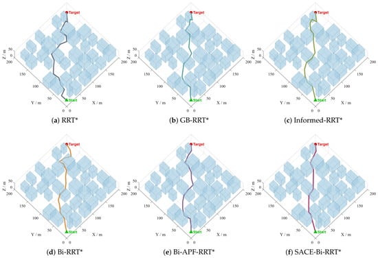
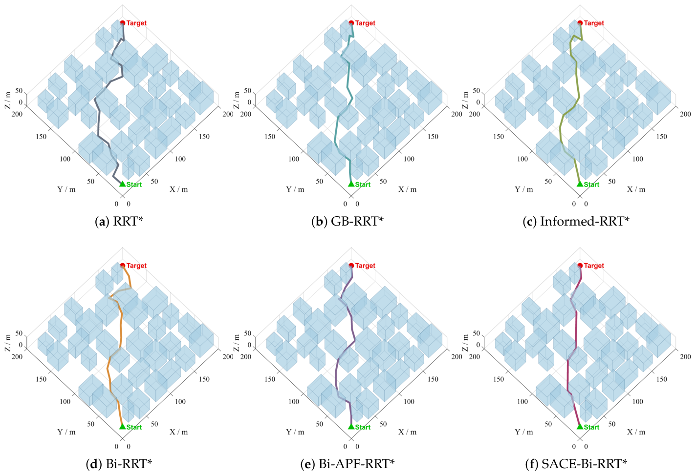
Figure 8 shows the planning results in the urban block. The three single-tree baselines enter and leave several streets before reaching the goal. Bi-APF-RRT* follows the street directions closely and deviates at the intersections, where the repulsion of the surrounding facades acts from both sides. SACE-Bi-RRT* crosses the network with its direction changes concentrated at the intersections.

Figure 8. Planning results of the six planners in the urban block. The single-tree planners (a–c) enter and leave several streets before reaching the goal; Bi-RRT* (d) passes between the buildings with several changes in direction; Bi-APF-RRT* (e) follows the street directions closely but deviates at the intersections, where the repulsion of the facades acts from both sides; and SACE-Bi-RRT* (f) traverses the street network with its direction changes concentrated at the intersections.

The number of iterations in Table 2 responds to this change in scene asymmetrically. Every baseline needs more iterations here than in the pillar forest, 1014 to 1420 compared with 592 to 854, and Bi-APF-RRT* needs 1420, the largest count of any algorithm in the three environments. SACE-Bi-RRT* converges in 527 iterations, which is 37.1% to 52.0% of the counts of the baselines and fewer than the 554 it needs in the pillar forest. Its final path length is 68.7% of that of RRT*, 71.1% and 71.5% of those of the two goal-directed single-tree baselines, 78.9% of that of Bi-RRT* and 83.6% of that of Bi-APF-RRT*. The margin is therefore wider against every baseline than in the pillar forest, while the ordering of the five baselines is unchanged. The dispersion gap is the wider of the two structured scenes, as the standard deviation of SACE-Bi-RRT* is 3.4 m and that of the baselines is 3.6 to 13.5 times as large. The average turning angle of SACE-Bi-RRT* is 33.4° here, more than the 20.4° of the pillar forest. This increase is not specific to the proposed planner. All six algorithms turn more sharply here than in the pillar forest, from 39.0° to 44.2° for Bi-APF-RRT* and from 52.2° to 54.0° for RRT*, since a path through a street network cannot avoid the turns that the network itself imposes. SACE-Bi-RRT* converges in 0.408 s on average, while the baselines need 0.049 s to 0.180 s.

5.3. Large-Scale Mixed Environment

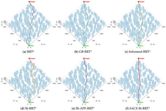
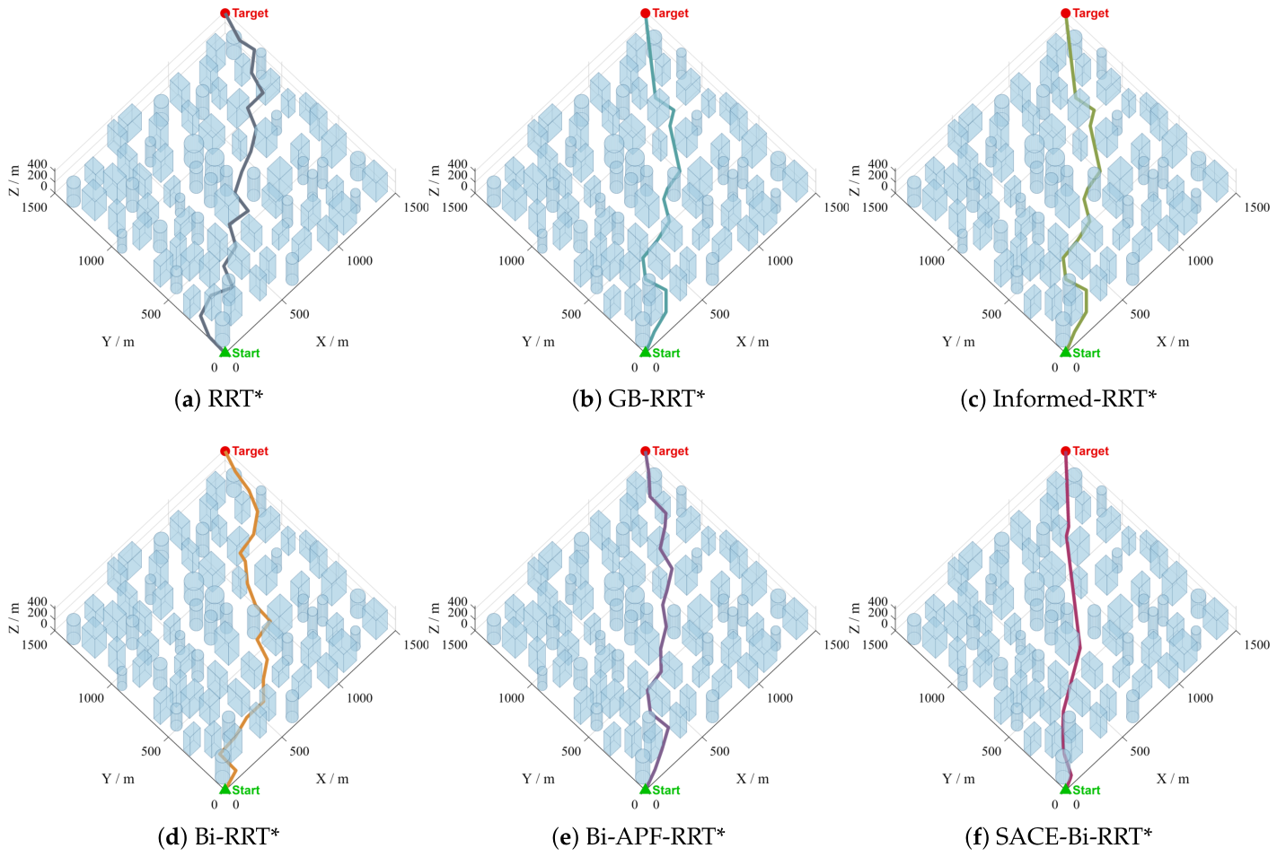
Figure 9 shows the planning results in the large mixed environment. The five baselines deviate at the clustered obstacle groups and recover their heading only after passing them, whereas the path of SACE-Bi-RRT* stays close to the start-to-goal direction between the groups.

Figure 9. Planning results of the six planners in the large-scale mixed environment. The paths of the five baselines (a–e) deviate at the clustered obstacle groups and recover their heading only after passing them, whereas SACE-Bi-RRT* (f) stays close to the start-to-goal direction between the groups.

The comparison in Table 2 turns on how the algorithms respond to the change in scale. Although the workspace is an order of magnitude larger, SACE-Bi-RRT* converges in 540 iterations, which lies within the range of 527 to 554 that it needs in the two structured scenes. The baselines need 772 to 1247 iterations, so its number of iterations is 43.3% to 70.0% of theirs. The average final path length of SACE-Bi-RRT* is 2215.2 m, which is 70.3% of that of RRT*, about 74.5% of those of the two goal-directed single-tree baselines, 80.2% of that of Bi-RRT* and 86.2% of that of Bi-APF-RRT*. Its average turning angle is 24.6°, and that of the baselines is 1.7 to 2.2 times as large. Convergence takes 0.622 s on average, against 0.037 s to 0.210 s for the baselines. These values indicate that the search effort of the proposed planner does not grow with the workspace at this scale, whereas that of every baseline does.

The baselines are dispersed here as well. Their path-length standard deviation grows to between 99.8 m and 260.9 m, which is 4.9 to 12.8 times the 20.3 m of SACE-Bi-RRT*.

5.4. Run-to-Run Stability

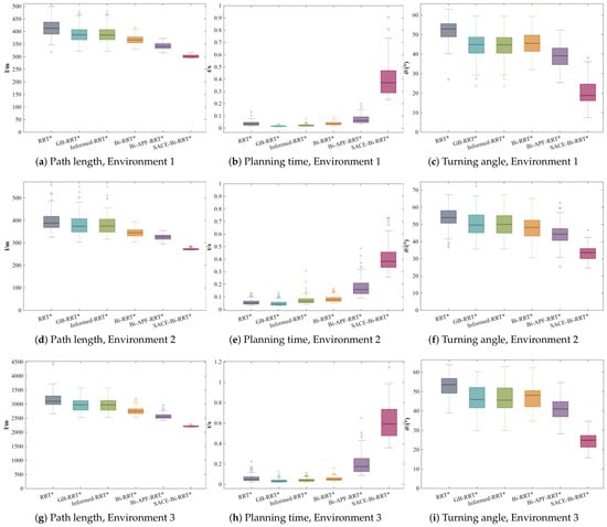
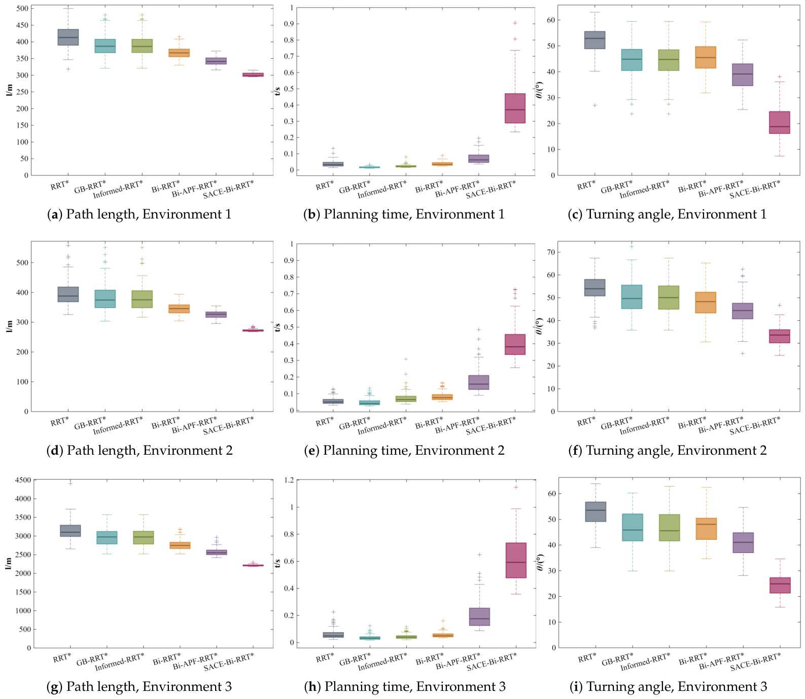
The preceding two subsections report each indicator as a mean and a standard deviation, and this subsection examines how the 100 runs are distributed around those means. Two views of the same data are used. Table 3 lists the coefficient of variation of the path length, defined as the ratio of the standard deviation to the mean, and Figure 10 gives the box plots of the path length, the planning time and the average turning angle for the six algorithms in the three environments.

Table 3. Coefficient of variation (%) of the path length over the 100 runs.

Algorithm	Environment 1	Environment 2	Environment 3
RRT*	$8.78$	$11.20$	$8.28$
GB-RRT*	$8.21$	$12.05$	$7.75$
Informed-RRT*	$8.20$	$11.28$	$7.93$
Bi-RRT*	$4.71$	$5.92$	$4.83$
Bi-APF-RRT*	$3.81$	$3.76$	$3.88$
SACE-Bi-RRT*	$1.88$	$1.26$	$0.92$

Figure 10. Box plots of the path length, the planning time and the average turning angle over the 100 runs. (a–c) Environment 1. (d–f) Environment 2. (g–i) Environment 3.

The coefficient of variation separates the six algorithms into three groups, and the same grouping holds in all three environments. It is 7.75% to 12.05% for the three single-tree baselines, 3.76% to 5.92% for the two bidirectional baselines and 0.92% to 1.88% for SACE-Bi-RRT*. Within the single-tree group, the three baselines exchange positions from one environment to another, whereas the order between the three groups is preserved. The distance to the most consistent baseline widens as the environment grows, since the coefficient of variation of Bi-APF-RRT* is 2.0 times that of SACE-Bi-RRT* in the pillar forest, 3.0 times in the urban block and 4.2 times in the large mixed environment.

To test whether the observed differences are statistically reliable, the runs are paired by seed, since run k of every planner uses the same random seed, and the final path length and the average turning angle of SACE-Bi-RRT* are compared with those of each baseline by the paired Wilcoxon signed-rank test. The Holm correction is applied to the five comparisons within each metric and environment. All 30 comparisons are significant at a Holm-adjusted $p<0.001$. Percentile bootstrap 95% confidence intervals of the means, based on 10,000 resamples, are reported in Table 4; the interval for SACE-Bi-RRT* does not overlap that of any baseline for either metric in any environment.

Table 4. Final path length and average turning angle over 100 runs (mean [95% CI]).

Environment	Algorithm	Path Length (m) Mean [95% CI]	Turning Angle (∘) Mean [95% CI]
Pillar forest	RRT*	$413.5[406.5,420.5]$	$52.2[51.1,53.2]$
	GB-RRT*	$388.9[382.9,395.3]$	$44.5[43.2,45.7]$
	Informed-RRT*	$388.9[382.8,395.3]$	$44.4[43.2,45.6]$
	Bi-RRT*	$367.9[364.5,371.3]$	$45.6[44.5,46.7]$
	Bi-APF-RRT*	$342.9[340.3,345.4]$	$39.0[37.8,40.1]$
	SACE-Bi-RRT*	$301.5[300.4,302.6]$	$20.4[19.2,21.6]$
Urban block	RRT*	$396.8[388.2,405.7]$	$54.0[52.8,55.1]$
	GB-RRT*	$383.7[374.9,393.0]$	$50.3[48.8,51.8]$
	Informed-RRT*	$381.3[373.2,389.9]$	$50.0[48.6,51.5]$
	Bi-RRT*	$345.6[341.6,349.6]$	$48.2[46.9,49.5]$
	Bi-APF-RRT*	$326.1[323.7,328.5]$	$44.1[42.9,45.4]$
	SACE-Bi-RRT*	$272.7[272.1,273.4]$	$33.4[32.6,34.3]$
Large mixed	RRT*	$3151.8[3102.2,3205.9]$	$53.0[51.9,54.0]$
	GB-RRT*	$2970.2[2925.0,3015.3]$	$46.3[45.0,47.6]$
	Informed-RRT*	$2973.9[2927.9,3020.3]$	$46.1[44.8,47.5]$
	Bi-RRT*	$2763.1[2737.4,2790.2]$	$46.9[45.8,48.0]$
	Bi-APF-RRT*	$2570.9[2551.4,2590.9]$	$41.1[40.0,42.2]$
	SACE-Bi-RRT*	$2215.2[2211.4,2219.3]$	$24.6[23.8,25.4]$

Figure 10 shows the same contrast run by run. The boxes of SACE-Bi-RRT* for the path length and the turning angle are the lowest and the most compact in every environment, and their whiskers stay short in the large mixed environment, where the boxes of all five baselines widen. The margins reported for the three environments are therefore carried by the whole distribution rather than by a subset of favorable runs. The planning-time boxes of SACE-Bi-RRT* lie above those of the baselines and stay narrow, so the additional computation listed in Table 2 varies little from one run to the next. For a planner that serves as the front end of a trajectory tracker, a path whose length and smoothness vary little across runs is as relevant as the average value of either quantity.

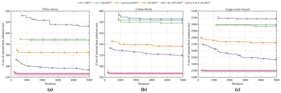
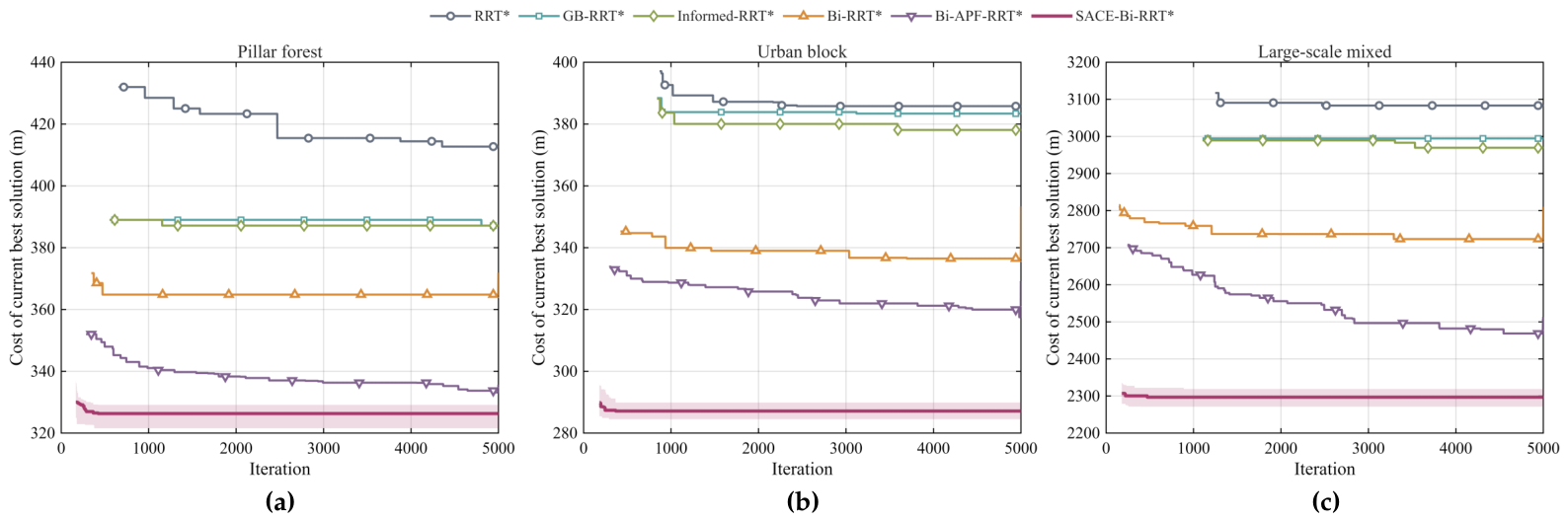
Figure 11 provides an empirical finite-iteration profile of the search. Each curve is the median cost of the current best solution over 30 seed-matched runs under a common 5000-iteration cap; for each planner, the curve begins at the first iteration at which all 30 runs have found a feasible solution. The shaded band shows the interquartile range for SACE-Bi-RRT*, and the plotted quantity is the best search-stage connection cost before the final shortcut post-processing. The proposed planner reaches a low cost early and then changes little, whereas the strongest baseline continues to improve gradually. This profile characterizes the observed anytime behavior within the tested iteration budget and is not a claim of asymptotic optimality.

Figure 11. Empirical evolution of the current best search cost under a common iteration cap of 5000. Each curve shows the median over 30 seed-matched runs, and plotting begins at the first iteration at which all runs of the corresponding planner have found a feasible solution. The shaded band shows the interquartile range of SACE-Bi-RRT*. The plotted cost is the current best connection cost before the final shortcut post-processing. (a) Pillar forest. (b) Urban block. (c) Large-scale mixed environment.

5.5. Discussion

The proposed components divide into two pairs. The gated guidance selects how often an extension aims at the opposite tree, and the tangent-plane deflection determines where that extension goes once it is blocked, so this pair fixes the direction. The bridge test selects which samples are worth an extension, and the adaptive step sets how far an accepted edge reaches, so this pair fixes its extent. A single extension of the full planner therefore carries the direction of the opposite tree, the local surface geometry of whatever blocks it, and the local clearance around it. A fixed-step random extension carries none of the three, which is consistent with the fewer iterations the planner needs to reach its stopping criterion in all three environments.

The tangent-plane deflection admits a direct comparison with the two nearest alternatives. The potential-field steering of Bi-APF-RRT* forms a resultant of goal attraction and obstacle repulsion at every extension, so its direction depends on the repulsion coefficient and on the distance to every obstacle in the neighborhood. In the street network of Environment 2, the facades on both sides of a street contribute opposing repulsions that can nearly cancel at an intersection. The tangent-plane deflection instead acts only when an extension is blocked, and it projects the intended direction onto the tangent plane of the contacted surface. The corrected direction is therefore determined by the geometry of the single surface that blocks the extension, rather than by a balance of forces over every obstacle in the neighborhood. The K-direction scan reaches the same result by sampling a fan of candidate directions around the blocked one and testing each, which returns the same path quality within 0.3% while evaluating eight candidates where the closed form evaluates five.

The final length advantage is next decomposed into the contribution of the search stage and that of the post-processing stage, over 30 runs per environment, and Table 5 reports both conditions as the mean and the standard deviation together with the reduction of SACE-Bi-RRT* relative to Bi-RRT*. In the raw condition, both planners return the merged path at the first connection, and the path of SACE-Bi-RRT* is 8.1%, 16.5% and 16.1% shorter in Environments 1 to 3, which isolates the effect of the guided expansion, the deflection, the adaptive step and the seam-cost connection. In the unified condition, the identical multi-round greedy shortcut is applied to both outputs. Except in the pillar forest, where the advantage narrows to 2.8%, the search-stage improvements survive the shortcut, and the advantage remains 13.8% and 10.2% in the urban block and in the large mixed environment. The pillar forest contains wide free corridors, so a large part of the redundancy of a raw path is recoverable by the shortcut alone, while in the street network and in the large mixed environment, the shortcut cannot move a path across an obstacle.

Table 5. Decomposition of the length advantage into the search stage and the post-processing stage (lengths in m).

Environment	Planner	Raw Length (m)	Unified Length (m)
Environment 1	Bi-RRT*	$354.06\pm 18.90$	$309.59\pm 10.62$
	SACE-Bi-RRT*	$325.22\pm 5.49$	$300.81\pm 5.48$
	Advantage	8.1%	2.8%
Environment 2	Bi-RRT*	$344.44\pm 18.35$	$316.55\pm 14.52$
	SACE-Bi-RRT*	$287.49\pm 4.49$	$272.97\pm 3.16$
	Advantage	16.5%	13.8%
Environment 3	Bi-RRT*	$2735.95\pm 123.41$	$2469.51\pm 120.94$
	SACE-Bi-RRT*	$2295.70\pm 32.81$	$2218.13\pm 18.77$
	Advantage	16.1%	10.2%

The guided extension is applied with probability at most $P_{max}=0.3$, leaving at least 70% of the iterations for global scrambled-Sobol sampling; the adaptive step is bounded below by ${\eta }_{min}>0$, and the rewiring radius follows Equation (3). These safeguards preserve a global-exploration branch that retains full support over the free space, together with a positive lower bound on the step, but they do not establish a formal probabilistic-completeness or asymptotic-optimality result for the complete planner. Accordingly, Figure 11 provides an empirical characterization of the search behavior within the tested finite iteration budget.

The higher planning time of SACE-Bi-RRT* is attributable to the additional operations introduced in its search and connection stages. During tree expansion, local clearance is queried to adapt the step size, and, when an extension is blocked, the surface normal is queried to compute a tangent-plane deflection. The planner also maintains the closest visible pair between the two trees. At the connection stage, it evaluates $K_c$ cross-tree candidate pairs using the seam cost and then applies a greedy shortcut to the merged path. Table 2 reports the resulting times: the mean first-solution times of SACE-Bi-RRT* are $0.082$, $0.085$ and $0.142$ s in Environments 1–3, respectively, and the mean converged times are $0.404$, $0.408$ and $0.622$ s. The five baselines require $0.003$–$0.027$ s for the first solution and $0.017$–$0.210$ s at convergence. Thus, the proposed planner incurs a higher planning-time cost in exchange for shorter and smoother paths. This trade-off makes it suitable for pre-flight global planning and low-rate global replanning, whereas high-frequency reactive avoidance is typically handled by a local planner. As an anytime planner, it can return the best path available when a prescribed iteration limit is reached.

6. Conclusions

In most existing bidirectional RRT* planners, the connection stage continuously measures the gap between the two trees and the visibility across it, yet this information is excluded from the extension decisions. At the same time, the local geometry exposed by a colliding extension is discarded outright. To overcome these deficiencies, this paper proposes the SACE-Bi-RRT* algorithm for path planning in three-dimensional static environments. In the guidance stage, a dual-tree guided expansion strategy is designed, in which the probability and the target of the guided extension are regulated jointly by the incrementally maintained closest node pair between the two trees and its line-of-sight visibility. During collision handling, a tangent-plane deflection strategy is introduced, which projects the blocked extension direction onto the tangent plane of the hit obstacle, thereby converting the collision into a deterministic detour along the obstacle surface. For the extension, an adaptive step-size strategy is employed to regulate the step length according to the clearance of the expanding node and its distance to the extension target. In the sampling stage, scrambled Sobol sequences are adopted to supply low-discrepancy exploratory samples, and an in-obstacle-triggered bridge test is incorporated to detect narrow passages. Finally, the two trees are merged at the candidate pair with the minimum seam cost, and a multi-round greedy shortcut is applied to shorten the merged path.

The planner is evaluated in three simulated three-dimensional environments, namely a pillar forest, an urban block scene, and a large-scale mixed map, with 100 independent runs per algorithm. In all three environments, SACE-Bi-RRT* returns shorter final paths than RRT*, goal-biased RRT*, Informed-RRT*, Bi-RRT* and the potential-field guided Bi-APF-RRT*, and the dispersion of its path lengths across repeated runs is markedly lower than that of every baseline. The planned paths also exhibit smaller average turning angles, so the improvement in length does not come at the expense of smoothness. The ablation study identifies the tangent-plane deflection strategy as the component most critical to the search efficiency, whereas the adaptive step-size strategy contributes mainly to the final path quality.

Nevertheless, several limitations remain in the present study, and the corresponding future research directions are outlined as follows:

(1) Computational overhead: The online geometric queries and the incremental maintenance of the connection information raise the per-iteration cost of SACE-Bi-RRT* above that of the lightweight baselines, which is reflected in the reported wall-clock times. Future research will reduce this overhead through spatial indexing and vectorized geometric queries and will profile the computational performance of the planner on embedded platforms.

(2) Problem scope: The planner treats the vehicle as a point mass in static environments composed of parametric primitives, and path smoothness is evaluated only a posteriori through the turning angle. Future research will incorporate kinematic constraints and curvature-continuous smoothing, introduce online replanning against dynamic obstacles, and extend the geometric queries to general obstacle representations such as triangle meshes and signed distance fields. Because the deflection uses only the clearance and normal queries, this extension requires replacing those two queries; future work will also investigate online adaptation of the deflection-score weights from local obstacle density.

(3) Simulation-based evaluation: All experiments were performed in MATLAB simulation, where the sensing errors, actuation delays, and external disturbances of a physical vehicle were not modeled. Future research will embed the planner in an onboard perception and control pipeline and validate it on a physical platform. The evaluation will also be extended to planner-compatible three-dimensional maps derived from public datasets such as the Newer College Dataset.

References

- Gugan, G.; Haque, A. Path Planning for Autonomous Drones: Challenges and Future Directions. Drones 2023, 7, 169. [Google Scholar] [CrossRef] [Scilit]
- Aggarwal, S.; Kumar, N. Path planning techniques for unmanned aerial vehicles: A review, solutions, and challenges. Comput. Commun. 2020, 149, 270–299. [Google Scholar] [CrossRef] [Scilit]
- Wang, D.; Zhang, M.; Huang, Z. A Path-Planning Method Recommended for Multi-UAV Police Patrols Based on the Wolf Pack Optimization Algorithm Using CDRS and DRSS. Symmetry 2025, 17, 208. [Google Scholar] [CrossRef] [Scilit]
- Liu, Y.; Liu, H.; Tian, Y.; Sun, C. Reinforcement learning based two-level control framework of UAV swarm for cooperative persistent surveillance in an unknown urban area. Aerosp. Sci. Technol. 2020, 98, 105671. [Google Scholar] [CrossRef] [Scilit]
- Colomina, I.; Molina, P. Unmanned aerial systems for photogrammetry and remote sensing: A review. ISPRS J. Photogramm. Remote Sens. 2014, 92, 79–97. [Google Scholar] [CrossRef] [Scilit]
- Fernandez Galarreta, J.; Kerle, N.; Gerke, M. UAV-based urban structural damage assessment using object-based image analysis and semantic reasoning. Nat. Hazards Earth Syst. Sci. 2015, 15, 1087–1101. [Google Scholar] [CrossRef] [Scilit]
- Liu, X.; Nardari, G.V.; Cladera, F.; Tao, Y.; Zhou, A.; Donnelly, T.; Qu, C.; Chen, S.W.; Romero, R.A.F.; Taylor, C.J.; et al. Large-Scale Autonomous Flight With Real-Time Semantic SLAM Under Dense Forest Canopy. IEEE Robot. Autom. Lett. 2022, 7, 5512–5519. [Google Scholar] [CrossRef] [Scilit]
- Chiella, A.C.B.; Machado, H.N.; Teixeira, B.O.S.; Pereira, G.A.S. GNSS/LiDAR-Based Navigation of an Aerial Robot in Sparse Forests. Sensors 2019, 19, 4061. [Google Scholar] [CrossRef] [Scilit]
- Mohta, K.; Watterson, M.; Mulgaonkar, Y.; Liu, S.; Qu, C.; Makineni, A.; Saulnier, K.; Sun, K.; Zhu, A.; Delmerico, J.; et al. Fast, autonomous flight in GPS-denied and cluttered environments. J. Field Robot. 2018, 35, 101–120. [Google Scholar] [CrossRef] [Scilit]
- Rashid, A.T.; Ali, A.A.; Frasca, M.; Fortuna, L. Path planning with obstacle avoidance based on visibility binary tree algorithm. Robot. Auton. Syst. 2013, 61, 1440–1449. [Google Scholar] [CrossRef] [Scilit]
- Kumar, P.; Pal, K.; Govil, M.C. Comprehensive Review of Path Planning Techniques for Unmanned Aerial Vehicles (UAVs). ACM Comput. Surv. 2026, 58, 1–44. [Google Scholar] [CrossRef] [Scilit]
- Goerzen, C.; Kong, Z.; Mettler, B. A Survey of Motion Planning Algorithms from the Perspective of Autonomous UAV Guidance. J. Intell. Robot. Syst. 2010, 57, 65–100. [Google Scholar] [CrossRef] [Scilit]
- Hart, P.E.; Nilsson, N.J.; Raphael, B. A Formal Basis for the Heuristic Determination of Minimum Cost Paths. IEEE Trans. Syst. Sci. Cybern. 1968, 4, 100–107. [Google Scholar] [CrossRef] [Scilit]
- Harabor, D.; Grastien, A. Online Graph Pruning for Pathfinding on Grid Maps. In Proceedings of the Twenty-Fifth AAAI Conference on Artificial Intelligence, San Francisco, CA, USA, 7–11 August 2011; AAAI Press: Menlo Park, CA, USA, 2011; pp. 1114–1119. [Google Scholar] [CrossRef] [Scilit]
- Nash, A.; Koenig, S.; Tovey, C. Lazy Theta*: Any-Angle Path Planning and Path Length Analysis in 3D. In Proceedings of the Twenty-Fourth AAAI Conference on Artificial Intelligence, Atlanta, GA, USA, 11–15 July 2010; AAAI Press: Menlo Park, CA, USA, 2010; pp. 147–154. [Google Scholar] [CrossRef] [Scilit]
- Jiang, Y.; Xu, X.-X.; Zheng, M.-Y.; Zhan, Z.-H. Evolutionary computation for unmanned aerial vehicle path planning: A survey. Artif. Intell. Rev. 2024, 57, 267. [Google Scholar] [CrossRef] [Scilit]
- LaValle, S.M. Rapidly-Exploring Random Trees: A New Tool for Path Planning; Technical Report TR 98-11; Department of Computer Science, Iowa State University: Ames, IA, USA, 1998. [Google Scholar]
- Karaman, S.; Frazzoli, E. Sampling-based algorithms for optimal motion planning. Int. J. Robot. Res. 2011, 30, 846–894. [Google Scholar] [CrossRef] [Scilit]
- Orthey, A.; Chamzas, C.; Kavraki, L.E. Sampling-Based Motion Planning: A Comparative Review. Annu. Rev. Control Robot. Auton. Syst. 2024, 7, 285–310. [Google Scholar] [CrossRef] [Scilit]
- Zhu, L.; Duan, P.; Meng, L.; Yang, X. GAO-RRT*: A path planning algorithm for mobile robot with low path cost and fast convergence. AIMS Math. 2024, 9, 12011–12042. [Google Scholar] [CrossRef] [Scilit]
- Guan, T.; Han, Y.; Kong, M.; Wang, S.; Feng, D.; Yang, W. An improved artificial potential field with RRT star algorithm for autonomous vehicle path planning. Sci. Rep. 2025, 15, 16982. [Google Scholar] [CrossRef] [Scilit]
- Gammell, J.D.; Srinivasa, S.S.; Barfoot, T.D. Informed RRT*: Optimal sampling-based path planning focused via direct sampling of an admissible ellipsoidal heuristic. In Proceedings of the 2014 IEEE/RSJ International Conference on Intelligent Robots and Systems, Chicago, IL, USA, 14–18 September 2014; IEEE: New York, NY, USA, 2014; pp. 2997–3004. [Google Scholar] [CrossRef] [Scilit]
- Huang, C.; Tang, B.; Guo, Z.; Su, Q.; Gai, J. Agile-RRT*: A Faster and More Robust Path Planner With Enhanced Initial Solution and Convergence Rate in Complex Environments. IEEE Access 2024, 12, 58703–58714. [Google Scholar] [CrossRef] [Scilit]
- Zhao, S.; Han, P.; Diao, Z.; He, Z.; Li, X.; Lou, T.; Jiang, L. Improved Informed RRT*: Based on Dynamic Shrinkage Threshold Node Selection Mechanism and Adaptive Goal-Biased Strategy. Electronics 2025, 14, 648. [Google Scholar] [CrossRef] [Scilit]
- Zhao, X.; Wang, K.; Zhang, P.; Kan, J. An improved RRT* path planning algorithm combining Gaussian distributed sampling and depth strategy for robotic arm of fruit-picking robot. Comput. Electron. Agric. 2026, 240, 111244. [Google Scholar] [CrossRef] [Scilit]
- Zhong, H.; Cong, M.; Wang, M.; Du, Y.; Liu, D. HB-RRT: A path planning algorithm for mobile robots using Halton sequence-based rapidly-exploring random tree. Eng. Appl. Artif. Intell. 2024, 133, 108362. [Google Scholar] [CrossRef] [Scilit]
- Zhong, H.; Du, Y.; Liu, D.; Wang, M.; Cong, M.; Tian, X. A fruit fly-inspired path planning algorithm for unmanned aerial vehicle in underground environments based on low-discrepancy sequences. Eng. Appl. Artif. Intell. 2025, 156, 111250. [Google Scholar] [CrossRef] [Scilit]
- Kuffner, J.J.; LaValle, S.M. RRT-Connect: An Efficient Approach to Single-Query Path Planning. In Proceedings of the 2000 IEEE International Conference on Robotics and Automation, San Francisco, CA, USA, 24–28 April 2000; IEEE: New York, NY, USA, 2000; pp. 995–1001. [Google Scholar] [CrossRef] [Scilit]
- Jordan, M.; Perez, A. Optimal Bidirectional Rapidly-Exploring Random Trees; Technical Report MIT-CSAIL-TR-2013-021; MIT Computer Science and Artificial Intelligence Laboratory: Cambridge, MA, USA, 2013. [Google Scholar]
- Wilson, T.S.; Thomason, W.; Kingston, Z.; Gammell, J.D. AORRTC: Almost-Surely Asymptotically Optimal Planning with RRT-Connect. IEEE Robot. Autom. Lett. 2025, 10, 13375–13382. [Google Scholar] [CrossRef] [Scilit]
- Huang, Y.; Jiang, W.; Xu, S. A multi strategy bidirectional RRT* algorithm for efficient mobile robot path planning. Sci. Rep. 2025, 15, 29501. [Google Scholar] [CrossRef] [Scilit]
- Chen, D.; Luo, K.; Wang, Z.; Fan, L.; Wang, C. An adaptive bidirectional optimal rapidly exploring random tree algorithm with dynamic adjustment and extended guidance strategy. Robot. Auton. Syst. 2026, 198, 105314. [Google Scholar] [CrossRef] [Scilit]
- He, X.; Zhou, Y.; Liu, H.; Shang, W. Improved RRT*-Connect Manipulator Path Planning in a Multi-Obstacle Narrow Environment. Sensors 2025, 25, 2364. [Google Scholar] [CrossRef] [Scilit]
- Zhang, M.; Liu, S.; Zhou, Q.; Han, X. A novel path planning scheme based on Fast-IBi-RRT* algorithm for industrial robots. Appl. Intell. 2025, 55, 785. [Google Scholar] [CrossRef] [Scilit]
- Nayak, S.; Otte, M.W. Bidirectional Sampling-Based Motion Planning Without Two-Point Boundary Value Solution. IEEE Trans. Robot. 2022, 38, 3636–3654. [Google Scholar] [CrossRef] [Scilit]
- Hu, Y.; Chen, X.; Tang, P.; Zhang, H.; Jin, J.; Mao, S. A Path Planning Framework for Robots Based on Improved Parallel Sampling RRT and Offset Guidance DWA. IEEE Sens. J. 2025, 25, 35597–35608. [Google Scholar] [CrossRef] [Scilit]
- Zhang, L.; Ling, Y.; Bing, Z.; Wu, F.; Haddadin, S.; Knoll, A. Tree-Based Grafting Approach for Bidirectional Motion Planning With Local Subsets Optimization. IEEE Robot. Autom. Lett. 2025, 10, 5815–5822. [Google Scholar] [CrossRef] [Scilit]
- Qureshi, A.H.; Ayaz, Y. Potential functions based sampling heuristic for optimal path planning. Auton. Robots 2016, 40, 1079–1093. [Google Scholar] [CrossRef] [Scilit]
- Zhang, X.; Wang, P.; Guo, Y.; Han, Q.; Zhang, K. Path Planning Algorithm for Manipulators in Complex Scenes Based on Improved RRT*. Sensors 2025, 25, 328. [Google Scholar] [CrossRef] [Scilit]
- Han, Q.; Ma, X.; Liu, H.; Xu, Y.; Xie, Y.; Yang, Q.; Meng, F. Improved Artificial Potential Field Method for UAV Path Planning. IEEE Access 2025, 13, 177537–177547. [Google Scholar] [CrossRef] [Scilit]
- Liu, C.; Xiao, F.; Ma, Y.; Chen, H.; Wu, Y.; Li, Z.; Guo, L. An enhanced RRT* algorithm with biased sampling and dynamic stepsize strategy for ship route planning in the high-risk areas. Ocean Eng. 2025, 332, 121466. [Google Scholar] [CrossRef] [Scilit]
- Wang, J.; Xiong, G.; Dang, B.; Chen, J.; Zhang, J.; Xie, H. Improved RRT-Based Obstacle-Avoidance Path Planning for Dual-Arm Robots in Complex Environments. Machines 2025, 13, 621. [Google Scholar] [CrossRef] [Scilit]
- Yu, Q.; Zhou, J.; Xue, Z. Path planning of manipulator considering obstacle avoidance based on improved RRT algorithm. J. Braz. Soc. Mech. Sci. Eng. 2025, 47, 505. [Google Scholar] [CrossRef] [Scilit]
Disclaimer/Publisher’s Note: The statements, opinions and data contained in all publications are solely those of the individual author(s) and contributor(s) and not of MDPI and/or the editor(s). MDPI and/or the editor(s) disclaim responsibility for any injury to people or property resulting from any ideas, methods, instructions or products referred to in the content. |
© 2026 by the authors. Licensee MDPI, Basel, Switzerland. This article is an open access article distributed under the terms and conditions of the Creative Commons Attribution (CC BY) license.