Feature Engineering for Queue Waiting Time Prediction: Temporal and Queue-State Reconstruction on the Theta Supercomputer

Abstract

Predicting queue waiting time for batch job schedulers in high-performance computing (HPC) systems is a critical research topic aimed at maximizing resource utilization efficiency and enhancing user experience. However, existing prediction approaches heavily rely on static job characteristics provided by users at submission time, exhibiting clear limitations in capturing the dynamic congestion state of the scheduling system. To address these limitations, a log-based feature engineering approach designed to significantly improve queue waiting time prediction accuracy is proposed in this study. Specifically, feature redundancy is eliminated through comparative analysis, and temporal features capturing periodic job submission patterns are generated. Furthermore, global and local (queue-level) waiting and running states at job submission time are reconstructed exclusively from historical job logs, thereby representing dynamic queue congestion in a fine-grained manner. The effectiveness of the proposed framework was validated using a large-scale job log dataset collected from the Theta supercomputer at the Argonne Leadership Computing Facility (ALCF) between 2017 and 2023, where queue waiting time was discretized into nine distinct intervals and formulated as a multi-class classification problem. Finally, an ablation study was conducted to quantitatively evaluate the performance contribution of each engineered feature group, and comparative experiments were carried out across multiple machine learning models, including Naïve Bayes, k-nearest neighbors (KNN), Random Forest, and XGBoost. Among the compared models, Random Forest achieved the best overall performance, with an accuracy of 88.89%, a balanced accuracy of 57.65%, a macro-averaged precision of 67.95%, and a macro-averaged F1-score of 61.71%. Compared with the baseline feature set, the proposed feature engineering strategy improved accuracy, balanced accuracy, and macro F1-score by 3.85, 7.28, and 9.82 percentage points, respectively, and the proposed RF model obtained a balanced accuracy 18 percentage points higher than the best-performing model reported in a comparable reference study on the same dataset, a cross-study difference not directly attributable to the proposed feature engineering alone.

1. Introduction

High-performance computing (HPC) systems, such as supercomputers, serve as essential infrastructure for a wide range of scientific and engineering domains that require large-scale computation, including weather forecasting, drug discovery, materials simulation, and artificial intelligence model training. These large-scale supercomputing systems are operated as clusters composed of numerous compute nodes, and their limited resources are shared among a large number of users. To enable fair and efficient resource utilization among multiple users, supercomputers are, in most cases, managed through a batch job scheduler. The batch job scheduler registers user-submitted jobs in a job queue and executes them in a determined order according to management policies. Specifically, the scheduler calculates job priorities based on scheduling policies applied by system administrators, such as first-in-first-out (FIFO) [1] or fairness-aware [2] scheduling, and sequentially dequeues jobs to be matched with available resources once sufficient resources become available, as determined through worker node status monitoring. The resulting queue waiting time, which inevitably arises from this process, is influenced by multiple factors acting in combination, including the scale of resources requested by the job (e.g., the number of nodes, cores, and the amount of memory), the applied queue policy, concurrent system load, and the processing status of preceding jobs. Owing to this combination of factors, queue waiting time exhibits substantial variability and is widely known to be difficult to predict [3,4].

Despite this difficulty, accurate prediction of queue waiting time is of considerable importance to both users and system administrators. From the user’s perspective, knowledge of the expected waiting time in advance enables proactive job planning, such as adjusting the job submission time or utilizing alternative resources. From the system administrator’s perspective, waiting time prediction information can be leveraged to improve scheduling policies and optimize resource allocation, ultimately enhancing overall system throughput and user satisfaction. Because queue waiting time prediction provides such valuable information to both users and administrators, numerous recent studies have addressed this problem using machine learning and deep learning techniques [5]. However, existing studies have largely relied on static job characteristics available at submission time, and have shown limitations in adequately capturing the dynamic congestion state of the scheduling system.

To overcome these limitations, a method is proposed in this study to improve prediction accuracy through various feature engineering techniques based on information available at job submission time. The central novelty of this study lies in the reconstruction of global and local queue-state information, that is, the number and resource footprint of jobs currently waiting and running, purely from historical job logs at the moment of submission, without requiring any scheduler-internal state or future information. Unlike prior feature-based studies, which have relied primarily on static job attributes declared by users at submission time, and prior time-based studies, which have modeled waiting time as a univariate temporal signal, the complementary information of these two perspectives is combined within a single feature engineering framework in this work. To the best of our knowledge, this is the first study to integrate periodicity-aware temporal features with fine-grained global and same-queue congestion reconstruction, and to quantify the contribution of each component through a controlled ablation study. Specifically, this study makes the following contributions:

• Periodicity-aware temporal feature generation: Temporal features at the year, month, day, day-of-week, hour, and minute granularity were derived from the job submission timestamp, enabling the prediction model to learn recurring job submission and resource utilization patterns that arise over annual, weekly, and daily cycles. Prior to this step, redundant features were removed through Pearson correlation analysis and mapping consistency analysis to obtain a compact baseline feature set.
• Log-based queue-state reconstruction: Queue states that are not explicitly recorded in scheduler logs were reconstructed as global and local (same-queue) waiting and running states. For each job, only the records of previously submitted jobs were referenced in a causal manner with respect to its submission time, from which 24 congestion features were derived, including the number of waiting jobs, the aggregated requested nodes and cores, and the requested walltime statistics. Queue congestion at job submission time is thereby represented in a more fine-grained manner.
• Quantitative attribution of feature group contributions: Through an ablation study in which the feature set was progressively expanded, the contribution of each feature group to prediction performance was isolated and quantified. In particular, it was experimentally confirmed that temporal and queue-state features improve not only the performance on the majority class, but also the detection of long-waiting minority classes, which are of greater operational importance.

The effectiveness of the proposed feature engineering approach was validated using large-scale job log data (DIM_JOB_COMPOSITE) collected from the Theta supercomputer at the Argonne Leadership Computing Facility (ALCF) between 2017 and 2023. Queue waiting time was further formulated as a multi-class classification problem by discretizing it into nine intervals, and the performance of multiple machine learning models, including Naïve Bayes (NB), k-nearest neighbors (KNN), Random Forest (RF), and Extreme Gradient Boosting (XGBoost) [6], was compared to provide useful information for selecting a prediction model suited to the target system.

The remainder of this paper is organized as follows. Section 2 reviews related work on queue waiting time prediction, categorized into feature-based, time-based, and deep learning-based approaches. Section 3 describes the proposed methodology, including the feature engineering process, the model training procedure, and the evaluation metrics employed in this study. Section 4 presents the experimental results, comprising a comparison of machine learning models, an ablation study on the contribution of each feature group, and an evaluation of sequence modeling and time-series applicability. Finally, Section 5 concludes the paper and discusses directions for future work.

2. Related Work

Queue waiting time provides highly useful information for both operators and users of HPC cluster systems, and extensive research has therefore been conducted on this topic. Studies on queue waiting time prediction can be broadly categorized into three streams, according to the nature of the information employed for prediction. The first is the feature-based approach, in which the attributes of individual jobs are utilized as features. The second is the time-based approach, in which the temporal pattern of variation in waiting time itself is treated as the object of analysis. The third is the approach incorporating novel model architectures, including deep learning.

First, studies belonging to the feature-based prediction approach construct features from attributes available at the time of job submission (e.g., the number of requested nodes, walltime, queue type, and user information) and employ these features to predict waiting time [3,7,8,9]. In [3], the authors investigated the impact of job characteristics—such as queue type and resource requirements—on job wait times in leadership-class HPC systems, including the Theta and Polaris systems at Argonne National Laboratory. The study evaluated various supervised learning algorithms for wait time prediction and comprehensively assessed how data preprocessing techniques, including outlier detection, Principal Component Analysis (PCA), and feature selection, influence model performance. In [7], an integrated framework was developed that uses job characteristics, along with queue state and processor occupancy, to identify and predict quick starters, while existing strategies are used to predict jobs with long queue waiting times. Experimental results demonstrated that the proposed prediction strategies can lead to the correct identification of up to 20 times more quick starters and provide tighter bounds for these jobs, resulting in up to 64% higher overall prediction accuracy than existing methods. In [8], a machine learning (ML)-based methodology was presented for predicting the time that jobs submitted to an HPC batch scheduler have to wait before execution. Specifically, both unsupervised learning (UL) and supervised learning (SL) techniques were applied to define the most effective features for the prediction task and to predict the actual queue waiting time. Experimental results showed a strong relationship between the performance of the SL models and the way the dataset was split. At the end of the prediction step, an uncertainty quantification approach was presented, in which prediction values were associated with reliability metrics based on variance estimation. In [9], a queue waiting time prediction framework for meta-scheduling in parallel batch systems was proposed. In this method, a hierarchical prediction strategy is adopted, whereby the point waiting time of a job is first predicted using dynamic kNN, followed by multi-class classification using a support vector machine (SVM) to compute probabilities for the predicted class and its neighboring classes, thereby providing a probability-weighted waiting time range. Overall, feature-based approaches capture the influence of individual job attributes on waiting time but rely predominantly on information declared at submission time, and generally do not represent the dynamic congestion state of the scheduling system as it evolves over time.

The second category of studies focuses not on the attributes of individual jobs, but on the temporal variation of waiting time; that is, on how the state of the queue evolves over time [4,10,11,12,13,14]. Downey [10,11] explored a log-uniform distribution to model the remaining lifetimes of the jobs. It was shown that it is possible to predict the queue waiting time with accuracy if the scheduling algorithm is known. In [12], the authors proposed a method for predicting queue waiting time based on run-time prediction techniques. The core idea of the proposed method is to first predict the execution time of an application and then combine this predicted value with a scheduling algorithm to simulate the behavior of the scheduler, thereby deriving when a given job would begin execution; that is, how long it would wait in the queue. In [13], the QBETS (Queue Bounds Estimation from Time Series) method was proposed, which, rather than producing a point estimate of the exact waiting time of an individual job, predicts an upper bound on waiting time accompanied by a statistical confidence level. This method consists of three components: a clustering procedure that groups jobs with similar characteristics, a change-point detector that identifies transitions between stationary intervals, and a percentile estimator based on the Binomial Method that estimates quantiles from the history within each cluster. In particular, the Binomial Method was presented as a non-parametric approach that infers directly from the data without distributional assumptions. In [14], the performance of job execution time and queue waiting time prediction techniques was systematically evaluated in a grid environment using a trace-based approach. In particular, prediction performance was evaluated for simple and widely used time-series prediction techniques such as Exponential Smoothing, Running Mean, Sliding Median, Last, and Last2. In addition, a method for estimating waiting time based on predicted execution time, as well as a non-parametric method for predicting an upper bound on waiting time accompanied by a confidence level, was presented. In [4], a method for predicting queue waiting time based on a Hidden Markov Model was proposed. Specifically, the prediction method is divided into three steps. First, outliers are detected and removed through statistical analysis. Second, the temporal transition pattern is modeled using logs prior to time t, and the parameters of the hidden states are computed. Third, the state at time $t+1$ is predicted using the computed hidden state parameters. Experimental results demonstrated that the proposed method achieves a prediction performance improvement of up to 60%. While these time-based approaches effectively model the temporal evolution of queue congestion, they largely disregard job-specific attributes such as requested resources and queue type, limiting their ability to differentiate waiting time across heterogeneous job types. In addition, conventional time-based approaches often rely on the assumption of stationarity, whereas queue waiting time in actual environments frequently fails to satisfy this assumption [4].

Finally, studies incorporating deep learning architectures, extending beyond traditional statistical techniques or tree-based models, have recently emerged [15,16]. In [15], a framework for estimating job wait times in HPC scheduling queues was presented, leveraging historical job scheduling data and real-time system metrics. High accuracy in predicting wait times was demonstrated, achieving 94.2% reliability within a 10-min error margin with RF and Multi-Layer Perceptron (MLP) models. In [16], TROUT (Two-tiered Regression Over Unbalanced Time), a hierarchical deep learning approach for predicting job queue waiting time, was proposed for Purdue University’s Anvil HPC cluster. To address the severe skew present in the data, the proposed method employed a hierarchical neural network architecture composed of a binary classifier and a regression model. Specifically, the binary classification model determines whether a job is a quick-starting job expected to begin within 10 min, and only for jobs predicted to exceed 10 min does the regression model predict the specific waiting time. Although deep learning-based approaches achieve strong predictive performance by combining historical scheduling data with real-time metrics, they typically require substantially more training data and computational resources, and their internal representations offer limited interpretability compared with feature-based tree ensemble methods.

In this paper, as in [3], correlation analysis between queue waiting time and job features, together with feature analysis and the prediction performance of various machine learning techniques such as RF and XGBoost, is presented. However, the present paper is distinguished from the previous study in the following important aspects. First, the effectiveness of explicit sequence modeling was investigated by comparing a Long Short-Term Memory (LSTM) model with the best-performing non-sequential machine learning model using a reconstructed historical sequence dataset. The experimental results show that the performance of LSTM and the proposed RF model is comparable; however, because the observable sequence construction evaluated in this study disproportionately excludes long-waiting jobs, this finding is restricted to the specific sequence construction evaluated here and should not be generalized to sequence modeling for queue waiting-time prediction as a whole. Second, it was demonstrated through experiments that prediction performance can be improved through feature engineering involving the generation of additional variables. Finally, under a similar random-split evaluation setting, the proposed RF model achieved a higher balanced accuracy than the best-performing model reported in the previous study; however, because the two studies employ different feature representations and model configurations, this difference is reported as a cross-study performance comparison rather than as an improvement attributable solely to the method proposed in this paper.

3. Methodology

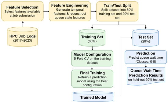
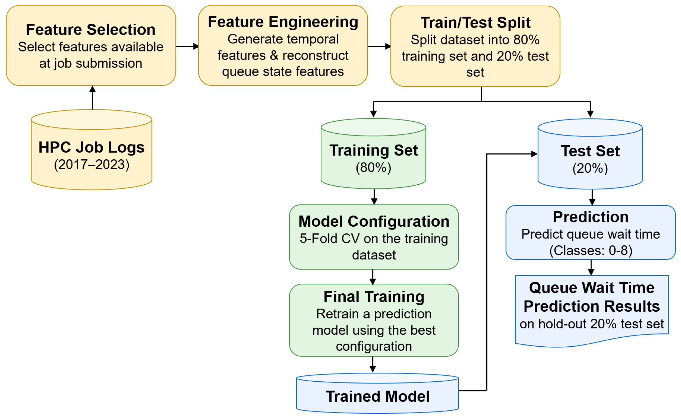
In this study, we investigated the impact of job characteristics and queue status on predicting queue waiting times for supercomputer jobs. We conducted a comparative analysis of multiple feature sets using historical supercomputer job log data, evaluating job characteristics available at submission time together with queue status information to identify the most informative features for improving prediction performance. The overall workflow of the proposed queue waiting time prediction framework is illustrated in Figure 1.

Figure 1. Overall workflow of the proposed queue waiting time prediction model.

3.1. Dataset

We utilized the DIM_JOB_COMPOSITE open dataset from the Theta supercomputer at the ALCF [17]. Theta is an 11.7-petaflop leadership-class HPC system based on the Intel-Cray XC40 architecture that supports large-scale scientific computing, data-intensive applications, and artificial intelligence workloads. This dataset contains historical job logs with job submission, start, and end timestamps, as well as job attributes such as requested resources and runtime information. These records allow us to derive temporal features (e.g., year, month, day of the week, hour of the day, and weekend indicator) and reconstruct the queue status at the time of job submission, thereby improving the prediction of queue waiting time. Table 1 presents the summary statistics of queue waiting times and requested computational resources for jobs submitted between 2017 and 2023. The dataset contains 540,503 jobs. Queue waiting time, which serves as the target variable in this study, shows large variation across all years. The overall mean waiting time is 577.84 min with a standard deviation of 3756.05 min, while the waiting time ranges from 0.02 to 296,908.20 min. The large standard deviation and the wide range between the minimum and maximum waiting times indicate that the target variable contains substantial variability and extreme waiting time values, making queue waiting time prediction a challenging task. In contrast, the requested computational resources, including nodes, cores, and walltime, remain relatively stable across different years.

Table 1. Annual summary statistics of submitted jobs and queue waiting times.

Year	Jobs	Mean Wait (min)	Wait SD (min)	Min Wait (min)	Max Wait (min)	Mean Requested Nodes	Mean Requested Cores	Mean Requested Walltime (min)
2017	54,801	156.30	1022.86	0.03	58,036.88	99.73	6382.42	165.60
2018	127,388	245.86	2313.57	0.03	296,908.20	110.00	7040.28	121.56
2019	91,342	507.58	3381.97	0.02	237,213.43	131.58	8420.95	106.76
2020	82,775	1222.37	5709.47	0.02	267,369.73	104.92	6714.76	107.54
2021	77,757	894.40	5470.28	0.02	272,749.33	124.65	7977.42	114.38
2022	62,520	623.10	3087.15	0.02	210,042.60	138.37	8855.54	115.59
2023	43,920	373.25	1861.55	0.25	80,750.20	138.01	8832.92	145.00
Overall	540,503	577.84	3756.05	0.02	296,908.20	119.49	7647.51	121.56

Only the information available at the time of job submission was considered as model input features to ensure that the proposed method can be deployed in real scheduling environments. Features requiring future information, such as the actual job start time, execution duration, and queue waiting time, were excluded. After removing features with more than 80% missing values and constant-valued features, 17 features remained as the baseline feature set. Table 2 summarizes the baseline features.

Table 2. Baseline features available at job submission.

Category	Feature	Description
Job Information	ALLOCATION_AWARD_CATEGORY	Allocation award category assigned to the job
	CAPABILITY	Job capability type
	MODE	The qsub command mode flag; script and interactive
	PROJECT_NAME_GENID	Project identifier
	QUEUE_NAME	Queue to which the job is submitted
	USERNAME_GENID	User identifier
Requested Resources	CORES_REQUESTED	Number of requested cores
	NODES_REQUESTED	Number of requested nodes
	WALLTIME_SECONDS	Requested walltime (s)
Application Information	IS_PYTHON	Whether the executable is a Python application
	REQUESTED_CORE_HOURS	Requested core-hours
	SCIENCE_FIELD	Sub Science field. The main science category with the sub category
	SCIENCE_FIELD_SHORT	The main science category without the sub category
	SIZE_BUCKETS3	Calculated job size bucket
	PERCENTILE	Percentile of job size
Submission Time	QUEUED_DATE_ID	Submission date identifier
	QUEUED_TIMESTAMP	Job submission timestamp

3.2. Feature Engineering

Feature engineering was performed to improve the model prediction performance of the queue waiting time. The process consisted of three main steps. First, feature redundancy analysis was conducted to identify and remove redundant features while retaining relevant information. Second, temporal features were generated from the job submission timestamp to capture temporal variations in job submission patterns. Third, queue state features were reconstructed from historical job records to represent the dynamic scheduling state at the time of job submission. The details of each step are described in the following subsections.

3.2.1. Feature Redundancy Analysis

Before training machine learning models, the feature redundancy analysis was conducted to identify highly correlated or semantically dependent features in the experimental HPC job log dataset. First, categorical variables were transformed into numerical representations to enable machine learning and statistical analysis. Binary features were encoded as 0/1 values, ordinal features were encoded according to their natural ordering, and nominal categorical features were label encoded. Different redundancy analysis methods were applied according to the characteristics of the features. Numerical feature redundancy was then evaluated using the Pearson correlation coefficient. Feature pairs with an absolute Pearson correlation coefficient greater than or equal to 0.9 were considered highly correlated and examined for redundancy. For nominal categorical features, Cramér’s V, a commonly used statistical measure for evaluating the strength of association between categorical variables [18], was used to avoid dependence on arbitrary numerical category labels. The association between SIZE_BUCKETS3 and CAPABILITY was evaluated using Cramér’s V. The resulting Cramér’s V was approximately 1.00, indicating an essentially perfect association between the two categorical variables. Therefore, SIZE_BUCKETS3 was considered redundant with CAPABILITY. The relationship between SCIENCE_FIELD and SCIENCE_FIELD_SHORT was evaluated using mapping consistency analysis. This analysis verified that each detailed scientific field mapped uniquely to a single broader scientific field, confirming that the two features represent the same semantic information at different levels. Table 3 summarizes the results of the mapping consistency analysis for SCIENCE_FIELD and SCIENCE_FIELD_SHORT, while Table 4 summarizes the redundant features identified through the different redundancy analyses.

Table 3. Mapping consistency analysis between SCIENCE_FIELD and SCIENCE_FIELD_SHORT.

Metric	Value
Unique SCIENCE_FIELD categories	46
Unique SCIENCE_FIELD_SHORT categories	15
Detailed fields mapped to multiple short fields	0
Many-to-one mapping verified	Yes

Table 4. Removed redundant features identified through feature redundancy analysis.

Removed Feature	Reason
SIZE_BUCKETS3	Perfect categorical association with CAPABILITY (Cramér’s $V\approx 1.00$).
PERCENTILE	Highly correlated with NODES_REQUESTED ($r=0.966$)
CORES_REQUESTED	Perfectly correlated with NODES_REQUESTED ($r=1.00$), indicating duplicate information.
SCIENCE_FIELD_SHORT	A grouped representation of SCIENCE_FIELD; mapping consistency analysis confirmed semantic redundancy.

Based on the redundancy analysis, SIZE_BUCKETS3, PERCENTILE, and CORES_REQUESTED were removed because they contained redundant information with other numerical features. The mapping consistency analysis further confirmed that SCIENCE_FIELD_SHORT is a grouped representation of SCIENCE_FIELD; therefore, only SCIENCE_FIELD was retained for model training.

3.2.2. Temporal Feature Generation

The submission timestamp of each job was used to derive temporal features that capture periodic patterns in job and resource utilization, which can differ across years, months, weekdays, and times of day, thereby influencing job waiting times. By incorporating temporal information, the prediction model can learn time-dependent variations in queue behavior that influence job waiting times. The generated temporal features from the QUEUED_TIMESTAMP feature are:

• YEAR: Submission year.
• MONTH: Submission month (1–12).
• DAY: Day of the month (1–31).
• DAY_OF_WEEK: Day of the week (Monday = 0, Sunday = 6).
• HOUR_OF_DAY: Hour of job submission (0–23).
• MINUTE: Minute of job submission (0–59).

3.2.3. Reconstruction of Queue State Features

In an operational HPC scheduling system, the current queue state, including which previously submitted jobs are waiting and which jobs are running, is directly observable by the scheduler when a new job is submitted. However, because such queue-state snapshots are not explicitly available in the historical workload log used in this study, we reconstructed the system state at each job submission time using the recorded submission, start, and completion events.

Specifically, for a target job submitted at time t, only previously submitted jobs were considered when constructing the queue-state features. The recorded START_TIMESTAMP and END_TIMESTAMP values of these previous jobs were used offline as event boundaries to determine whether each job was waiting, running, or completed at time t. These timestamps were therefore used to reconstruct the historical system state that existed at the target submission time and were not provided to the prediction model as input features. Instead, the prediction model receives aggregate features representing the reconstructed state, such as the numbers of waiting and running jobs and their requested nodes, cores, walltime, and related workload characteristics. This reconstruction is intended to reproduce the instantaneous queue-state information that would be directly observable from the scheduler in an online prediction setting.

Queue states were reconstructed by processing historical job records in ascending order of their submission timestamps. For each submitted job, the queue state at its submission time was reconstructed using only information from previously submitted jobs. These reconstructed features represent the dynamic state of the scheduling system at the time of job submission, allowing the prediction model to account for queue congestion and resource contention in addition to the current job attributes. To capture the dynamic state of the scheduling system at the time of job submission, four queue states were reconstructed: global waiting, global running, local waiting, and local running. The global states describe the overall status of the computing system, whereas the local states describe the status of the same queue (QUEUE_NAME) as that of the submitted job.

The local waiting and local running states were reconstructed using the same conditions as the corresponding global states, with the additional constraint that only jobs belonging to the same queue (QUEUE_NAME) as the current job were considered. The reconstructed queue state features are summarized in Table 5. The features are grouped according to their scope, either global or local.

Table 5. Reconstructed queue state features.

Feature	Description
Global queue state features
GLOBAL_WAITING_JOB_COUNT	Number of waiting jobs
GLOBAL_WAITING_NODES_SUM	Total requested nodes of waiting jobs
GLOBAL_WAITING_CORES_SUM	Total requested cores of waiting jobs
GLOBAL_WAITING_WALLTIME_MEAN	Mean requested walltime of waiting jobs
GLOBAL_WAITING_WALLTIME_MAX	Maximum requested walltime of waiting jobs
GLOBAL_WAITING_REQUESTED_CORE_HOURS_SUM	Total requested core-hours of waiting jobs
GLOBAL_WAITING_JOBS_GE_CURRENT_NODES	Number of waiting jobs requesting a number of nodes greater than or equal to that requested by the current job
GLOBAL_RUNNING_JOB_COUNT	Number of running jobs
GLOBAL_RUNNING_NODES_SUM	Total requested nodes of running jobs
GLOBAL_RUNNING_CORES_SUM	Total requested cores of running jobs
GLOBAL_RUNNING_WALLTIME_MEAN	Mean requested walltime of running jobs
GLOBAL_RUNNING_WALLTIME_MAX	Maximum requested walltime of running jobs
Local queue state features
LOCAL_WAITING_JOB_COUNT	Number of waiting jobs in the same queue
LOCAL_WAITING_NODES_SUM	Total requested nodes of waiting jobs in the same queue
LOCAL_WAITING_CORES_SUM	Total requested cores of waiting jobs in the same queue
LOCAL_WAITING_WALLTIME_MEAN	Mean requested walltime of waiting jobs in the same queue
LOCAL_WAITING_WALLTIME_MAX	Maximum requested walltime of waiting jobs in the same queue
LOCAL_WAITING_REQUESTED_CORE_HOURS_SUM	Total requested core-hours of waiting jobs in the same queue
LOCAL_WAITING_JOBS_GE_CURRENT_NODES	Number of waiting jobs in the same queue requesting a number of nodes greater than or equal to that requested by the current job
LOCAL_RUNNING_JOB_COUNT	Number of running jobs in the same queue
LOCAL_RUNNING_NODES_SUM	Total requested nodes of running jobs in the same queue
LOCAL_RUNNING_CORES_SUM	Total requested cores of running jobs in the same queue
LOCAL_RUNNING_WALLTIME_MEAN	Mean requested walltime of running jobs in the same queue
LOCAL_RUNNING_WALLTIME_MAX	Maximum requested walltime of running jobs in the same queue

To describe the reconstruction procedure formally, let $\mathcal{J}=\{1,\dots ,N\}$ denote the set of jobs sorted in ascending order of QUEUED_TIMESTAMP, and let job $c\in \mathcal{J}$ be the current job under consideration, submitted at time $t_c$. For any job j, let $q_j$, $s_j$, and $e_j$ denote its QUEUED_TIMESTAMP, START_TIMESTAMP, and END_TIMESTAMP, and let $n_j$, ${\mathrm{cr}}_j$, $w_j$, and ${\mathrm{ch}}_j$ denote its requested nodes, cores, walltime, and core-hours, respectively. The global waiting set $\mathcal{W}\left(c\right)$ and global running set $\mathcal{R}\left(c\right)$ at the submission time of job c are

$$\mathcal{W}\left(c\right)=\{j\in \mathcal{J}\left\{c\right\}:q_j<t_c,s_j>t_c\},\mathcal{R}\left(c\right)=\{j\in \mathcal{J}\left\{c\right\}:q_j<t_c,s_j<t_c,e_j>t_c\},$$

(1)

and the corresponding local sets, ${\mathcal{W}}_{\mathrm{loc}}\left(c\right)$ and ${\mathcal{R}}_{\mathrm{loc}}\left(c\right)$, are obtained by additionally requiring $\mathtt{QUEUE}\text{\_}{\mathtt{NAME}}_j=\mathtt{QUEUE}\text{\_}{\mathtt{NAME}}_c$. Every reconstructed feature in Table 5 is then an aggregate statistic over one of these four sets $\mathcal{S}\in \{\mathcal{W}\left(c\right),\mathcal{R}\left(c\right),{\mathcal{W}}_{\mathrm{loc}}\left(c\right),{\mathcal{R}}_{\mathrm{loc}}\left(c\right)\}$, computed using one of the following four operators:

$$\mathrm{Count}\left(\mathcal{S}\right)=\left|\mathcal{S}\right|,{\mathrm{Sum}}_x\left(\mathcal{S}\right)=\sum _{j\in \mathcal{S}}{x}_j,{\mathrm{Mean}}_x\left(\mathcal{S}\right)={\displaystyle \frac{1}{\left|\mathcal{S}\right|}}\sum _{j\in \mathcal{S}}{x}_j,{\mathrm{Max}}_x\left(\mathcal{S}\right)=\underset{j\in \mathcal{S}}{\max }{x}_j,$$

(2)

where $x_j\in \{n_j,{\mathrm{cr}}_j,w_j,{\mathrm{ch}}_j\}$ is the job-level attribute being aggregated (nodes, cores, walltime, or core-hours, respectively). For example, three representative features from Table 5 instantiate Equation (2) as follows:

$$\begin{array}{cc}\hfill \mathtt{GLOBAL}\text{\_}\mathtt{WAITING}\text{\_}\mathtt{JOB}\text{\_}\mathtt{COUNT}\left(c\right)& =\mathrm{Count}\left(\mathcal{W}\right(c\left)\right),\hfill \\ \hfill \mathtt{GLOBAL}\text{\_}\mathtt{WAITING}\text{\_}\mathtt{NODES}\text{\_}\mathtt{SUM}\left(c\right)& ={\mathrm{Sum}}_n\left(\mathcal{W}\left(c\right)\right),\hfill \\ \hfill \mathtt{LOCAL}\text{\_}\mathtt{RUNNING}\text{\_}\mathtt{WALLTIME}\text{\_}\mathtt{MAX}\left(c\right)& ={\mathrm{Max}}_w\left({\mathcal{R}}_{\mathrm{loc}}\left(c\right)\right).\hfill \end{array}$$

The single feature that is not a direct instance of Equation (2), GLOBAL_WAITING_JOBS_GE_CUR RENT_NODES (and its local counterpart), instead counts waiting jobs whose requested node count is at least that of the current job,

$$\mathtt{GLOBAL}\text{\_}\mathtt{WAITING}\text{\_}\mathtt{JOBS}\text{\_}\mathtt{GE}\text{\_}\mathtt{CURRENT}\text{\_}\mathtt{NODES}\left(c\right)=\sum _{j\in \mathcal{W}\left(c\right)}\mathbb{I}\left[n_j\ge n_c\right],$$

(3)

where $\mathbb{I}[·]$ is the indicator function, equal to 1 if the condition holds and 0 otherwise; this feature quantifies the number of comparably sized or larger jobs ahead of job c in the (global or local) queue, and is intended as a proxy for the resource contention that job c is likely to face.

3.2.4. Computational Complexity and Versatility

The queue-state reconstruction procedure described above operates entirely on job-level timestamps and requested-resource attributes and can be implemented as a single chronological pass over the job log. Given N historical jobs, the jobs are first sorted by QUEUED_TIMESTAMP, which requires $O\left(N\log N\right)$ time. The chronological pass then maintains the currently waiting and currently running jobs (globally, and separately per queue) in incrementally updatable data structures. Each job is inserted into the relevant waiting set when it is submitted and moved into the running set when it starts. Running aggregate statistics are updated incrementally as each job is inserted, transitioned, or evicted. Count and sum are updated in $O\left(1\right)$ time, while the maximum is maintained using a max-heap with lazy deletion. In this scheme, an evicted job is not removed from the heap immediately but is instead marked as stale in $O\left(1\right)$ time, and stale entries are discarded lazily from the top of the heap whenever the current maximum is queried. Consequently, each job is popped at most once over the course of the pass, and the amortized cost per insertion, transition, or eviction is $O\left(\log N\right)$. In addition, the count of waiting jobs requesting at least as many nodes as the current job is maintained using the binary indexed tree [19] indexed by requested node count, which supports both rank queries and updates in $O\left(\log N\right)$ time. Since each of the N jobs is inserted, transitioned, and evicted at most once, computing the full set of features requires $O\left(N\log N\right)$ time in total and $O\left(K\right)$ additional space.

In terms of versatility, the procedure requires only submission, start, and end timestamps, a queue or partition identifier, and the requested-resource fields (nodes, cores, walltime, and, where available, core-hours), information that is recorded by essentially all production batch schedulers (e.g., PBS, SLURM [20], and LSF), including the Theta scheduler logs used in this study. Because this procedure makes no assumption about the specific scheduling policy, queue configuration, or workload mix of the target system, it can be applied directly to job logs collected from other HPC systems.

3.2.5. Class Labeling

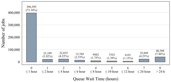
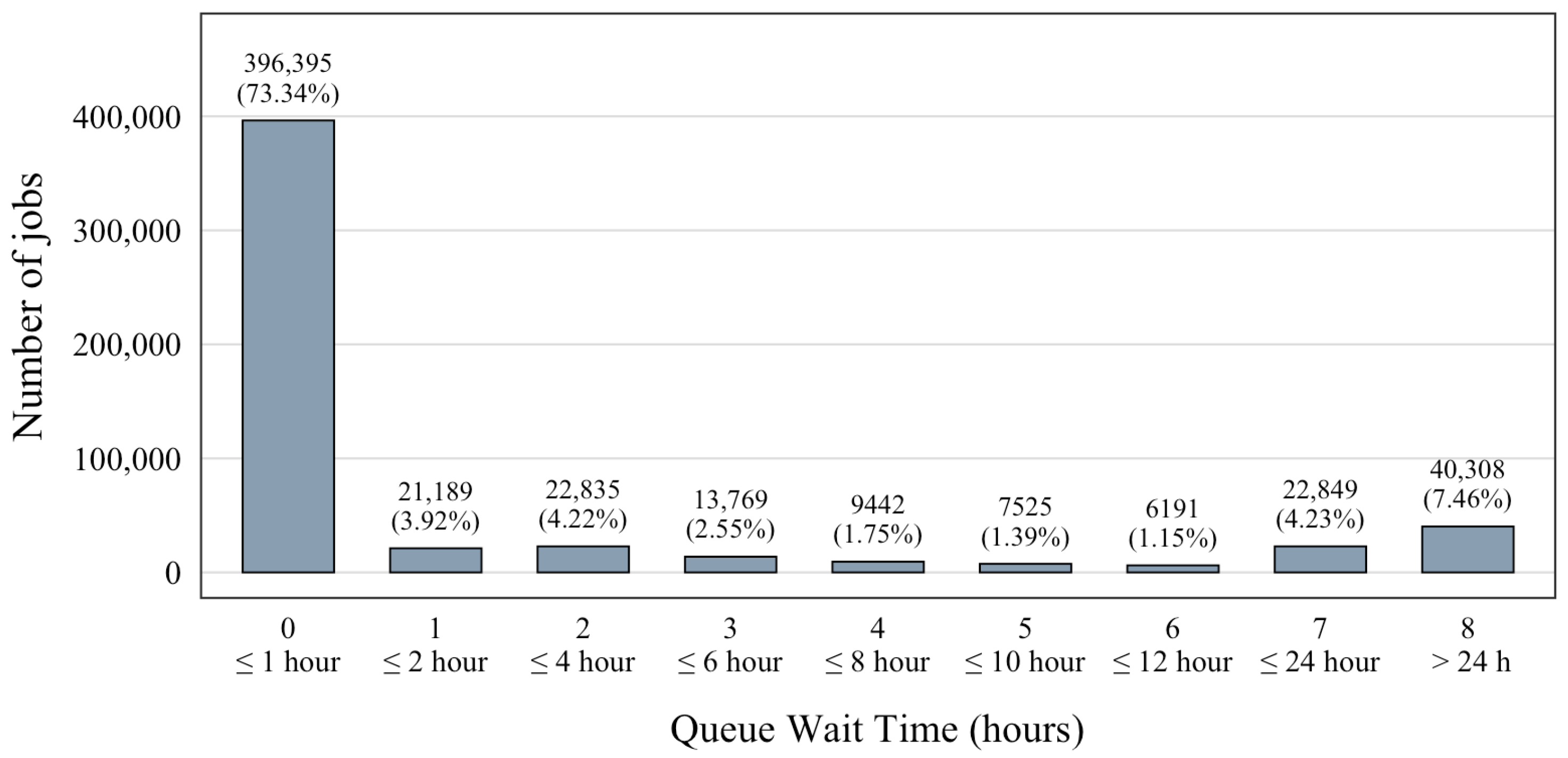
Queue waiting time (QUEUED_WAIT_SECONDS) was formulated as a multi-class classification problem. The continuous queue waiting time was converted from seconds to hours and partitioned into nine waiting time intervals, with each interval assigned a class label ranging from 0 to 8, as summarized in Table 6. The number and proportion of jobs in each class are listed in Table 6, and the corresponding class distribution is illustrated in Figure 2. The dataset presents a highly imbalanced class distribution, with Class 0 (≤1 h) containing the largest proportion of jobs, while the remaining classes contain relatively fewer jobs.

Table 6. Queue waiting-time class labels and class distribution.

Class	Wait Time (h)	Jobs	Proportion (%)
0	≤ 1	396,395	73.34
1	>1–≤2	21,189	3.92
2	>2–≤4	22,835	4.22
3	>4–≤6	13,769	2.55
4	>6–≤8	9442	1.75
5	>8–≤10	7525	1.39
6	>10–≤12	6191	1.15
7	>12–≤24	22,849	4.23
8	>24	40,308	7.46
Total		540,503	100.00

Figure 2. Distribution of jobs across the queue waiting time intervals.

As summarized in Table 6, the nine-class discretization scheme was adopted to match the interval boundaries used in [3], the most closely related prior work addressing the queue waiting time prediction task on the same Theta logs, thereby enabling a direct and fair comparison of classification performance between the two studies. Because classification performance is inherently sensitive to the granularity and placement of discretization boundaries, an independently derived binning scheme would have confounded differences in reported performance with differences in label definition rather than differences in modeling approach. Accordingly, the same nine intervals were adopted in the present study to ensure that the performance improvements observed relative to that prior work are attributable to the proposed method itself, rather than to a more favorable class definition.

3.2.6. Predictive Model Training

As shown in Figure 1, the processed dataset was divided into training and test sets using a random 80%/20% split. The training set was used for model configuration through five-fold cross-validation to determine the optimal hyperparameter configuration for the predictive model. After the optimal configuration was identified, the prediction model was retrained using the entire training set to obtain the final trained model. The trained model was then applied to the hold-out test set to predict the queue waiting time range based on class labels from 0 to 8. Finally, the prediction performance was evaluated using the performance metrics described in Section 3.2.7.

3.2.7. Evaluation Measurements

Due to the imbalanced class distribution of the HPC job log dataset, prediction performance was evaluated using accuracy, balanced accuracy, macro-averaged precision, and macro-averaged F1-score to assess overall classification performance across all classes.

Class 0 accounts for 73.34% of the observations, whereas the least represented class, Class 6, accounts for only 1.15%. No explicit resampling or class-balancing technique was applied during model training. Conventional accuracy measures the overall proportion of correctly classified samples. In contrast, balanced accuracy computes the average recall across all classes, making it less affected by class imbalance because each class contributes equally to the final score. Macro-averaged precision and macro-averaged F1-score were additionally used to evaluate model performance by computing the metric independently for each class and then averaging the resulting values across all classes. The prediction performance of the proposed model was evaluated using overall performance metrics (Accuracy, Balanced Accuracy, Macro-averaged Precision, and Macro-averaged F1-score) and per-class performance metrics (Precision, Recall, and F1-score). The evaluation metrics are described as follows:

• Accuracy: Conventional accuracy measures the proportion of correctly classified samples among all samples.

  $$\mathrm{Accuracy}={\displaystyle \frac{{\sum }_{i=1}^{C}T{P}_i}{N}}$$

  (4)

  where C is the total number of classes, $T{P}_i$ is the number of true positive predictions for class i, and N is the total number of samples.
• Balanced Accuracy: Balanced accuracy is defined as the average recall across all classes. Compared with conventional accuracy, balanced accuracy is less affected by class imbalance because each class contributes equally to the final score.

  $$\mathrm{Balanced} \mathrm{Accuracy}={\displaystyle \frac{1}{C}}{\displaystyle \sum _{i=1}^C}{\displaystyle \frac{T{P}_i}{T{P}_i+F{N}_i}}$$

  (5)

  where $F{N}_i$ is the number of false negative predictions for class i.
• Macro-averaged Precision: Macro-averaged precision is computed by calculating the precision for each class independently and then averaging the resulting values across all classes.

  $$\text{Macro-averaged} \mathrm{Precision}={\displaystyle \frac{1}{C}}{\displaystyle \sum _{i=1}^C}{\mathrm{Precision}}_i$$

  (6)
• Macro-averaged F1-score: Macro-averaged F1-score is computed by calculating the F1-score for each class independently and then averaging the resulting values across all classes.

  $$\text{Macro-averaged} \mathrm{F}1={\displaystyle \frac{1}{C}}{\displaystyle \sum _{i=1}^C}\mathrm{F}{1}_i$$

  (7)
• Precision, Recall, and F1-score: Precision, recall, and F1-score evaluate the prediction performance of each individual class. Precision measures the proportion of samples predicted as class i that are correctly classified. Recall measures the proportion of actual samples belonging to class i that are correctly classified. The F1-score is the harmonic mean of precision and recall.

  $${\mathrm{Precision}}_i={\displaystyle \frac{T{P}_i}{T{P}_i+F{P}_i}},$$

  (8)

  $${\mathrm{Recall}}_i={\displaystyle \frac{T{P}_i}{T{P}_i+F{N}_i}},$$

  (9)

  $$\mathrm{F}{1}_i={\displaystyle \frac{2\times {\mathrm{Precision}}_i\times {\mathrm{Recall}}_i}{{\mathrm{Precision}}_i+{\mathrm{Recall}}_i}}$$

  (10)

  where $F{P}_i$ is the number of false positive predictions for class i.

4. Experimental Analysis

To comprehensively evaluate the proposed approach, four complementary experiments were conducted. First, four machine learning algorithms, namely NB, KNN, RF, and XGBoost, were evaluated using the proposed feature set, which consisted of job characteristics, temporal features, and reconstructed queue state features, in order to identify the most suitable prediction model. Second, an ablation study was conducted to evaluate the contribution of individual feature groups. Third, the effectiveness of explicit sequence modeling was investigated by comparing a LSTM model with the best-performing non-sequential model using a reconstructed historical sequence dataset. Finally, the applicability of conventional time-series modeling to queue waiting-time prediction was investigated through individual-job and daily aggregated analyses.

4.1. Comparison with Classification Models

To identify the most suitable prediction model for queue waiting time prediction on the proposed feature set, we compared four representative machine learning algorithms: NB, KNN, RF, and XGBoost. Each model was trained using its optimal hyperparameter configuration determined during the model configuration process described in Section 3.2.6.

Hyperparameter optimization was performed using grid search with five-fold stratified cross-validation on the training data. Balanced accuracy was used as the model-selection criterion. Table 7 summarizes the evaluated hyperparameter values, the selected settings, and the corresponding best mean five-fold cross-validation balanced accuracy.

Table 7. Hyperparameter search ranges and selected settings for the evaluated machine learning models.

Model	Hyperparameter	Search Range	Selected Value	Best CV Score
NB	Variance smoothing	${10}^{-12}$, ${10}^{-11}$, ${10}^{-10}$, ${10}^{-9}$, ${10}^{-8}$, ${10}^{-7}$	${10}^{-12}$	0.2317
KNN	Number of neighbors k	3, 5, 7, 9, 11, 13, 15, 17, 19, 21, 23, 25	3	0.4720
XGBoost	Number of estimators	100, 150, 200, 250, 300	300	0.4989
RF	Number of trees	100, 150, 200, 250, 300	250	0.5574

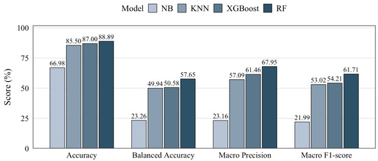
As depicted in Figure 3, the RF model achieved the highest performance across all evaluation metrics, including accuracy (88.89%), balanced accuracy (57.65%), macro precision (67.95%), and macro F1-score (61.71%).

Figure 3. Performance comparison of machine learning models for queue waiting time prediction.

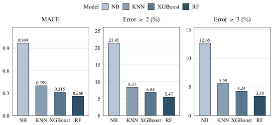
Ordinal error analysis: Although the prediction task was formulated as nine-class classification, the waiting-time classes are inherently ordered. Conventional multiclass classification metrics do not explicitly account for the distance between the actual and predicted classes. Therefore, additional ordinal error measures were calculated to evaluate the magnitude of prediction errors. The mean absolute class error (MACE) was calculated as:

$$\mathrm{MACE}={\displaystyle \frac{1}{N}}{\displaystyle \sum _{i=1}^N}\left|y_i-{\widehat{y}}_i\right|,$$

(11)

where $y_i$ and ${\widehat{y}}_i$ denote the actual and predicted class indices, respectively, and N is the number of test samples.

MACE represents the average distance, in number of classes, between the actual and predicted waiting-time classes. A lower MACE therefore indicates that the predicted classes are, on average, closer to the actual classes. In addition, severe-misclassification rates were calculated as the percentages of test samples for which the absolute class error was at least two classes ($|y_i-{\widehat{y}}_i|\ge 2$) and at least three classes ($|y_i-{\widehat{y}}_i|\ge 3$).

As shown in Figure 4, RF achieved the lowest MACE and the lowest severe-misclassification rates among the evaluated classifiers, followed by XGBoost. RF obtained a MACE of 0.260, while 5.47% and 3.38% of its predictions differed from the actual class by at least two and three classes, respectively. In comparison, XGBoost achieved a MACE of 0.315, with corresponding severe-error rates of 6.84% and 4.24%. The substantially larger errors obtained by NB are also reflected in its MACE of 0.969 and severe-error rates of 21.45% and 12.65%. Thus, the relative advantage of RF observed using the conventional classification metrics is also retained when the ordinal magnitude of prediction errors is considered.

Figure 4. Ordinal error analysis of the machine learning models.

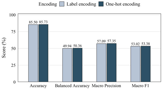
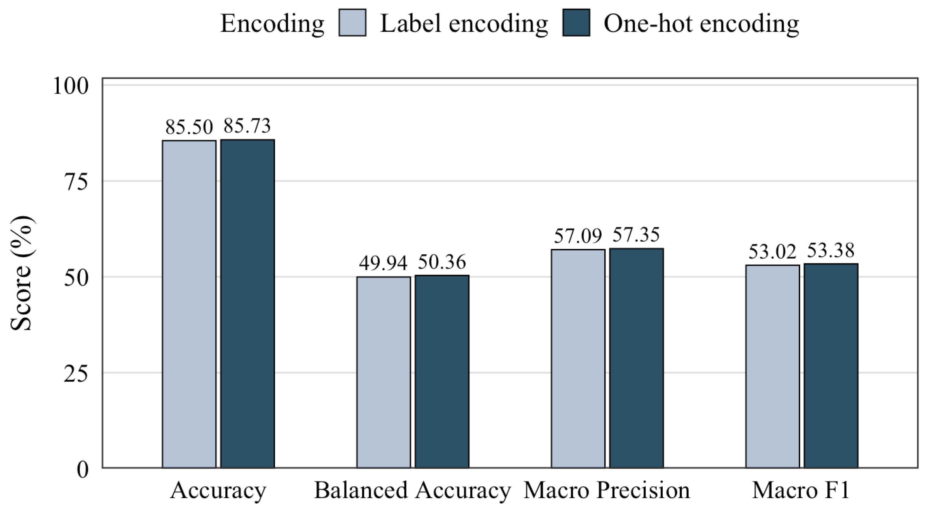
Sensitivity to categorical encoding: To examine the effect of categorical encoding on the distance-based KNN model, an additional experiment was conducted using one-hot encoding for categorical features. To isolate the effect of the encoding method, the same random 80/20 train–test split and the same number of neighbors ($k=3$) as in the original KNN experiment were retained. As shown in Figure 5, one-hot encoding resulted in only small improvements across the evaluated performance metrics, indicating that the overall KNN performance was relatively stable with respect to the categorical encoding method. Although one-hot encoding avoids the artificial numerical distances between nominal categories introduced by label encoding, it increased the transformed feature space to 2680 features, resulting in substantially higher computational and memory requirements for the distance-based KNN procedure.

Figure 5. KNN performance comparison using different categorical encoding methods.

Sensitivity to identity features: To evaluate the contribution of user- and project-specific identity information to the prediction performance, an additional feature ablation analysis was conducted using the RF model. The same random 80/20 train-test split and model configuration as in the original experiment were retained, while USERNAME_GENID and PROJECT_NAME_GENID were removed individually and jointly. As shown in Table 8, the model performance remained relatively stable across all feature configurations. In particular, balanced accuracy ranged from 57.65% to 57.71%, while macro F1-score ranged from 61.48% to 61.71%. Removing both identity variables resulted in only minor changes in the evaluated metrics. These results indicate that the contribution of the identity variables to the overall prediction performance is limited and that the model performance is primarily supported by the remaining job, resource-request, temporal, and queue-state features.

Table 8. Random Forest ablation analysis of user- and project-identity features.

Feature Configuration	Accuracy	Balanced Accuracy	Macro Precision	Macro F1
Full feature set	88.89%	57.65%	67.95%	61.71%
Without USERNAME_GENID	88.91%	57.71%	67.20%	61.48%
Without PROJECT_NAME_GENID	88.93%	57.71%	67.39%	61.55%
Without both identity features	88.91%	57.71%	67.18%	61.48%

Regression baseline: To provide an additional baseline that directly accounts for continuous queue waiting time, a Random Forest regression model was also evaluated. The regression model predicted queue waiting time in minutes using the same feature set and train-test partition as the classification experiment. It achieved a mean absolute error of 265.42 min.

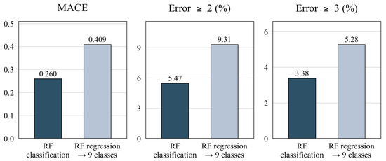
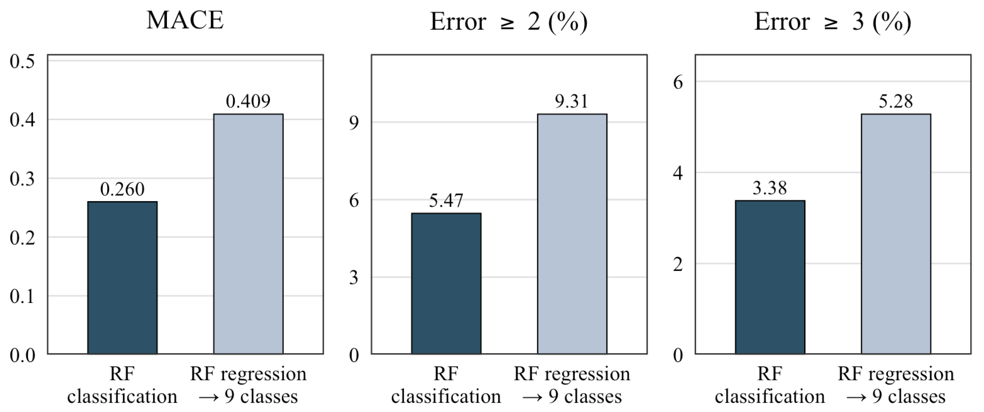
For comparison with the classification approach in the same ordinal class space, the continuous regression predictions were subsequently mapped to the same nine waiting-time intervals, after which MACE and the severe-misclassification rates were calculated. The results are presented in Figure 6.

Figure 6. Ordinal error comparison between RF classification and RF regression.

As shown in Figure 6, the RF classification model produced smaller ordinal errors than the RF regression baseline. The classification model achieved a lower MACE (0.260 versus 0.409), as well as lower severe-misclassification rates for errors of at least two classes (5.47% versus 9.31%) and at least three classes (3.38% versus 5.28%).

Temporal generalization evaluation: To assess temporal generalization, an additional chronological evaluation was conducted. All jobs were ordered according to QUEUED_TIMESTAMP, with the earliest 80% (432,402 jobs; June 2017–December 2021) used for model training and the latest 20% (108,101 jobs; December 2021–December 2023) retained for final model testing. Hyperparameter optimization was performed exclusively within the training portion using five-fold expanding-window cross-validation without shuffling.

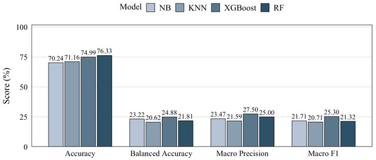
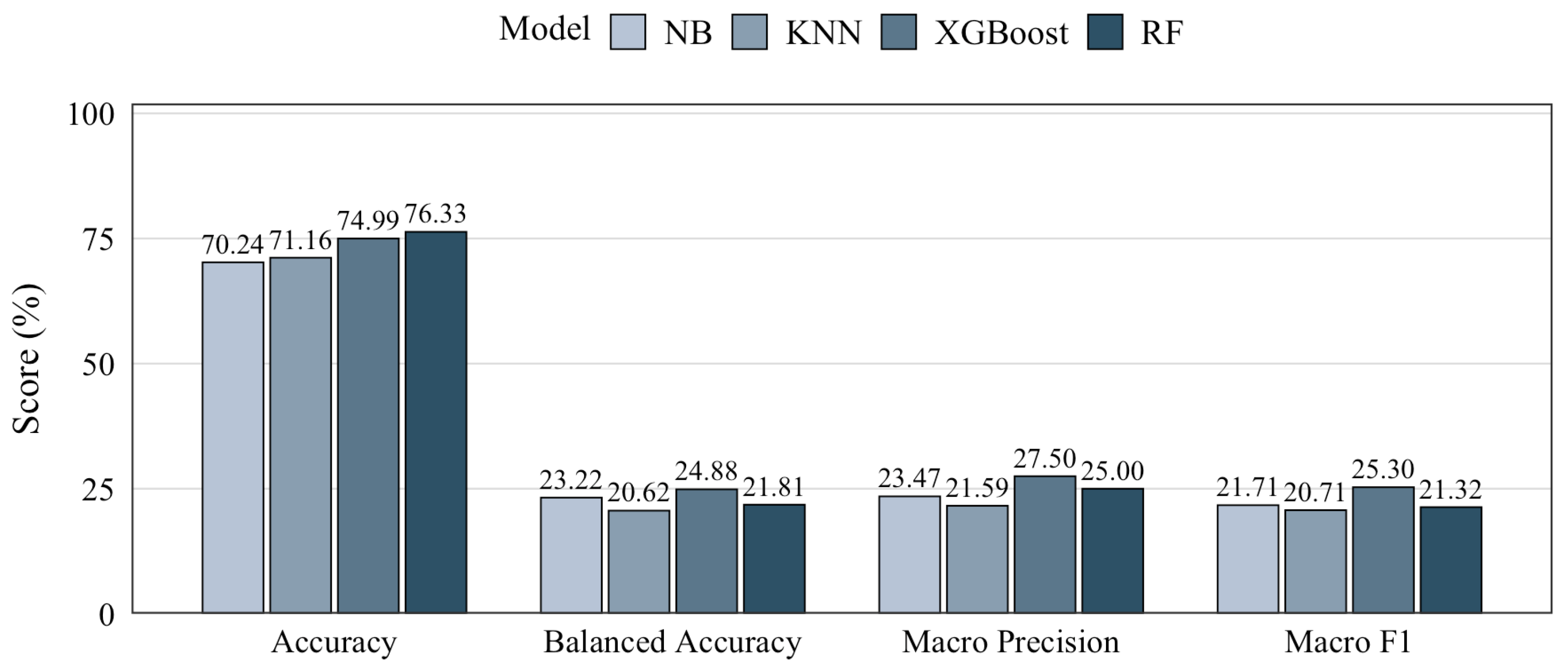
As shown in Figure 7, performance under the chronological evaluation was substantially lower than under the random-split evaluation, indicating that temporal changes in the workload affect out-of-time generalization. In addition, XGBoost achieved the highest balanced accuracy under the chronological setting, whereas RF achieved the highest performance in the random-split evaluation. This result indicates that the relative performance of the models is sensitive to temporal workload variation.

Figure 7. Performance comparison of machine learning models under chronological evaluation.

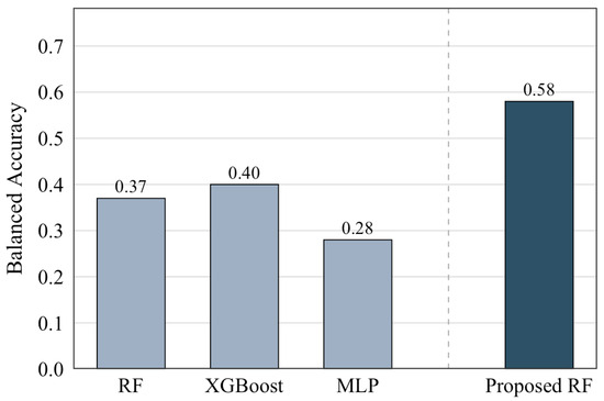
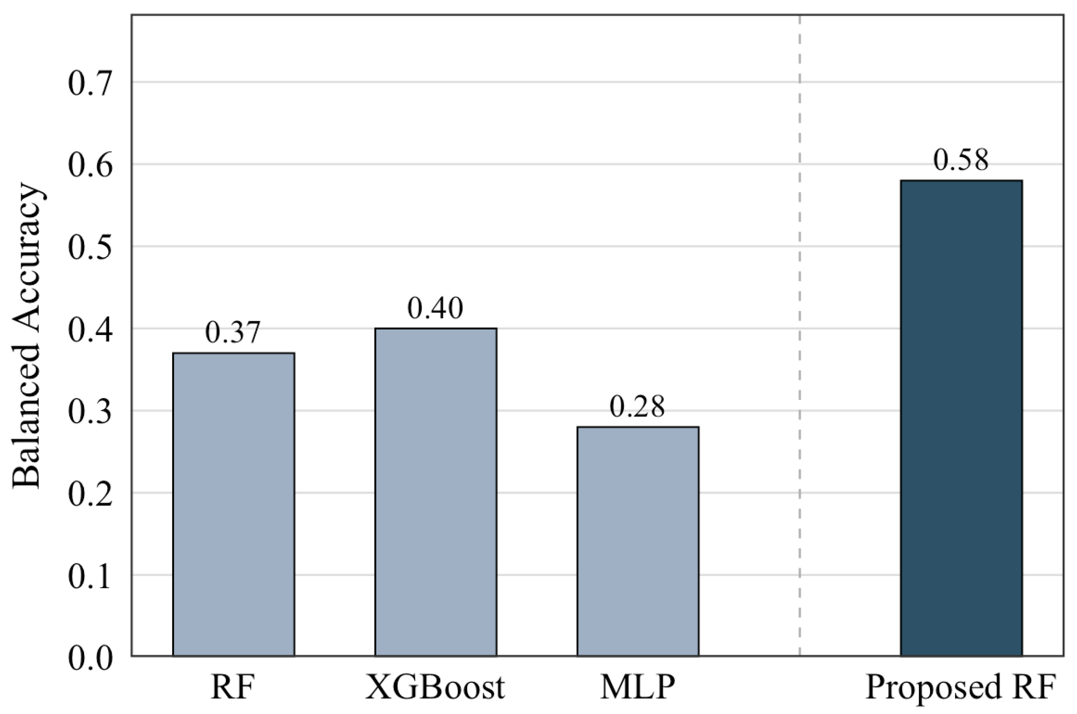
Comparison with the reference study: The performance of the proposed approach was compared with the results reported in [3]. Both the present study and [3] use the same Theta workload dataset, the same nine waiting-time class definitions, balanced accuracy as an evaluation metric, and random data partitioning with 20% of the data retained for testing. The proposed RF model achieved a balanced accuracy of 0.58, compared with 0.40 reported for the best-performing XGBoost model in [3], corresponding to an 18-percentage-point difference. However, because the two studies employ different train/test samples and model configurations, this difference should be interpreted as a cross-study performance comparison rather than as an improvement attributable solely to the proposed feature engineering. Figure 8 presents the reported balanced accuracy values from the two studies.

Figure 8. Comparison of balanced accuracy between the proposed RF model and the best-performing model reported in [3].

4.2. Feature Analysis Ablation Study

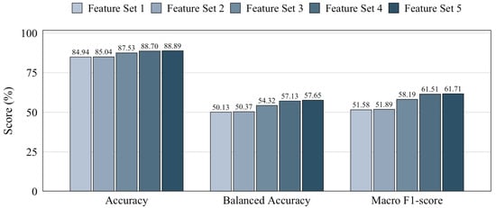
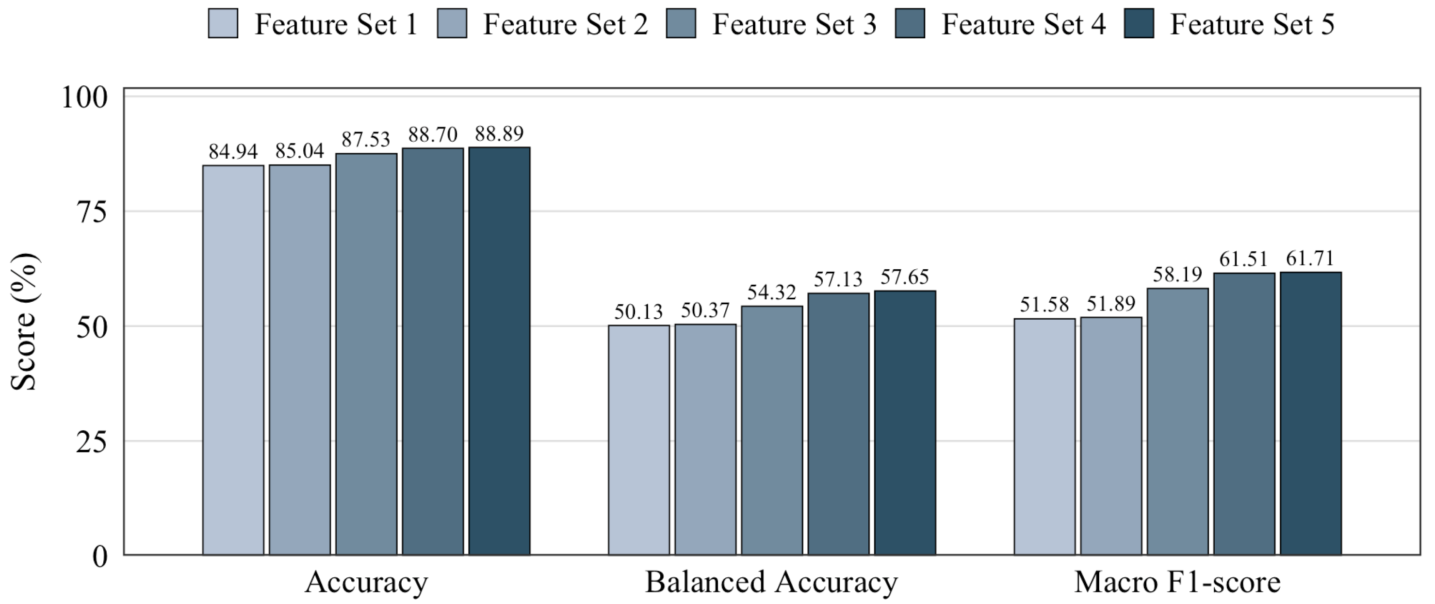
To evaluate the contribution of each feature set, we conducted an ablation study using five progressively enhanced feature sets shown in Table 9. Feature-Set 1 consists of the original features available at job submission time, as listed in Table 2. Feature-Set 2 removes highly correlated features (Pearson correlation > 0.9 and mapping consistency analysis) from Feature-Set 1. Feature-Set 3 combines Feature-Set 2 with temporal features generated from the job submission timestamp. Feature-Set 4 further incorporates global queue state features, while Feature-Set 5 (the proposed feature set) includes both global and local queue state features.

Table 9. Feature sets used in the ablation study.

Feature Set	Description
Feature-Set 1	Original features available at job submission time.
Feature-Set 2	Set 1 after removing highly correlated features.
Feature-Set 3	Set 2 + temporal features.
Feature-Set 4	Set 3 + global queue state features.
Feature-Set 5 (Proposed)	Set 4 + local queue state features.

Figure 9 illustrates the overall classification performance obtained using the five feature sets. Feature-Set 1, which contains the original features available at job submission time, achieved an accuracy of 84.94%, a balanced accuracy of 50.13%, and a macro F1-score of 51.58%. After removing features with high correlation, Feature-Set 2 produced nearly identical results. Accuracy increased slightly from 84.94% to 85.04%, while balanced accuracy and macro F1-score also improved from 50.13% to 50.37% and from 51.58% to 51.89%, respectively. These modest improvements suggest that removing highly correlated features reduced feature redundancy without losing predictive information. Although the performance gains were relatively small, the reduced feature set provides a more compact representation and was therefore selected as the baseline feature set for the subsequent experiments.

Figure 9. Overall classification performance for different feature sets in the ablation study.

The addition of temporal features in Feature-Set 3 resulted in a clear improvement in classification performance. Balanced accuracy and macro F1-score increased by 3.95% and 6.30%, respectively, indicating that temporal information contributed to improved discrimination of minority classes rather than only enhancing predictions for the dominant class. Feature-Set 4 further incorporated global queue state features. Compared with Feature-Set 3, this corresponds to improvements of 1.17% in accuracy, 2.81% in balanced accuracy, and 3.31% in macro F1-score. These results demonstrate that the global state of the queue provides useful contextual information for classification. Finally, Feature-Set 5, representing the complete proposed feature configuration, added local queue state features to Feature-Set 4. It achieved the highest performance across all metrics, with an accuracy of 88.89%, a balanced accuracy of 57.65%, and a macro F1-score of 61.71%. Compared with Feature-Set 4, the performance improvements were relatively small. Nevertheless, the consistent improvements across all evaluation metrics indicate that local queue state information provides complementary information beyond the global queue state. Overall, Feature-Set 5 improved accuracy by 3.85%, balanced accuracy by 7.28%, and macro F1-score by 9.82% compared to Feature-Set 2 (baseline). The larger improvements in balanced accuracy and macro F1-score indicate that the proposed feature-engineering strategy particularly enhanced performance across classes, including minority classes. Among the added feature groups, temporal and global queue state features provided the largest individual improvement, while local queue state features produced additional incremental gains.

Table 10 shows that the proposed Feature-Set 5 consistently outperforms the baseline Feature-Set 2 across all waiting-time classes. Averaged over the nine classes, precision, recall, and F1-score increase by approximately 14.19%, 7.28%, and 9.82%, respectively. This indicates that the additional engineered features improve the model’s ability to identify jobs belonging to each waiting-time category.

Table 10. Class-wise comparison between the baseline (Feature Set 2) and the proposed method (Feature Set 5). The difference ($\mathsf{\Delta }$) denotes the absolute improvement of the proposed method over the baseline.

Class	Precision (%)			Recall (%)			F1-Score (%)
	Baseline	Proposed	$\mathbf{\Delta }$	Baseline	Proposed	$\mathbf{\Delta }$	Baseline	Proposed	$\mathbf{\Delta }$
0	94.00	94.45	+0.45	96.63	98.86	+2.23	95.30	96.60	+1.31
1	43.68	68.14	+24.46	33.53	40.28	+6.75	37.94	50.63	+12.69
2	50.21	65.72	+15.51	44.78	54.57	+9.79	47.34	59.62	+12.29
3	44.27	62.55	+18.29	38.13	47.68	+9.55	40.97	54.11	+13.14
4	40.37	58.48	+18.11	35.54	42.37	+6.83	37.80	49.14	+11.34
5	36.57	56.02	+19.44	31.76	39.60	+7.84	34.00	46.40	+12.40
6	37.66	56.76	+19.10	35.62	39.34	+3.72	36.61	46.47	+9.86
7	57.95	68.86	+10.91	53.37	65.03	+11.66	55.56	66.89	+11.33
8	79.21	80.61	+1.40	84.00	91.12	+7.12	81.54	85.54	+4.01

The improvement in recall is particularly important because higher class labels represent longer queue waiting times. Correctly identifying these classes helps provide earlier warnings of long queue delays. For Classes 6–8, the proposed feature set improves recall by an average of approximately 7.50%. Class 7 recall increases from 53.37% to 65.03%, while Class 8 recall increases from 84.00% to 91.12%. These results demonstrate that the proposed approach effectively improves the detection of jobs that are likely to encounter long waiting times. The improved F1-score indicates that the increase in recall was achieved without a large loss in precision. Therefore, Feature-Set 5 provides a better balance between precision and recall for the operationally important long-waiting classes.

For precision, it increases by 19.10% for Class 6 and by 10.91% for Class 7. This means that jobs predicted as belonging to these long-waiting categories are more likely to be correctly classified. Although the precision improvement for Class 8 is small, its high precision is retained while recall increases substantially. This is important because Class 8 represents the most severe waiting-time condition, for which missing a truly delayed job is more costly than producing a limited number of false delay predictions.

Overall, the class-wise results suggest that incorporating temporal and queue state features is especially beneficial for distinguishing jobs with moderate-to-long queue waiting times. The improved recall and F1-score in the higher classes support the practical usefulness of the proposed feature set for the early detection of severe queue delays and more reliable waiting-time prediction.

4.3. Evaluation of Sequence Modeling

Although the proposed feature set already incorporates temporal and queue-state information, it does not explicitly model sequential dependencies. Therefore, an additional experiment was conducted to investigate whether explicit sequence modeling provides additional predictive benefits over the proposed feature-based non-sequential approach.

To evaluate the effectiveness of sequence modeling, an observable queue waiting-time sequence dataset was reconstructed from the original Theta HPC job log dataset. The jobs were first ordered chronologically according to their submission times. For each submitted job, only the waiting times of previously submitted jobs that had already begun execution by the current job’s submission time were considered observable. The waiting times of the three most recent observable jobs were arranged chronologically to form the input sequence (Lag-1 to Lag-3), which served as the sequential input to the LSTM-based classification model, together with the job features available at the current job’s submission time. The model was trained using the Adam optimizer with the sparse categorical cross-entropy loss function. The reconstructed dataset was divided into training and testing sets using an 80/20 chronological train-test split. The model was trained for 100 epochs using a batch size of 64.

Based on its superior performance in the previous experiments, RF was selected as the representative non-sequential baseline. RF was trained on the reconstructed dataset with and without the historical lag features to enable a fair comparison with the LSTM model.

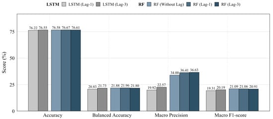
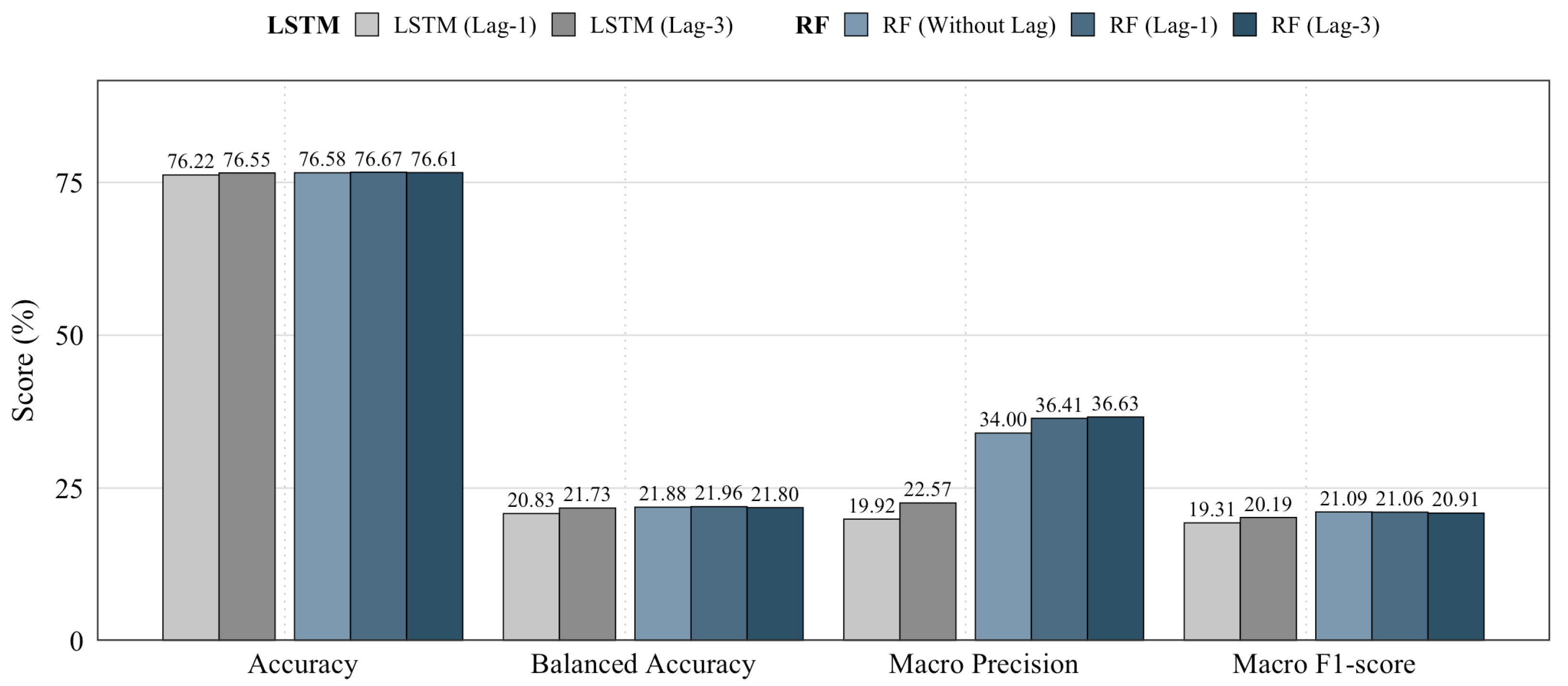
Figure 10 summarizes the performance of the LSTM and RF models on the reconstructed dataset. The results indicate that incorporating historical queue waiting-time information provides only marginal performance improvements for both models. For the LSTM model, increasing the sequence length from Lag-1 to Lag-3 slightly improved Accuracy (76.22% to 76.55%), Balanced Accuracy (20.83% to 21.73%). Similarly, RF exhibited only negligible performance changes after incorporating the historical lag features, with the Lag-1 configuration achieving the highest Accuracy (76.67%) and Balanced Accuracy (21.96%).

Figure 10. Performance comparison of LSTM and RF using different historical sequence lengths.

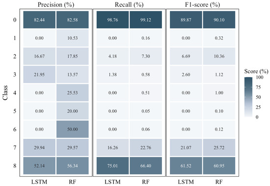
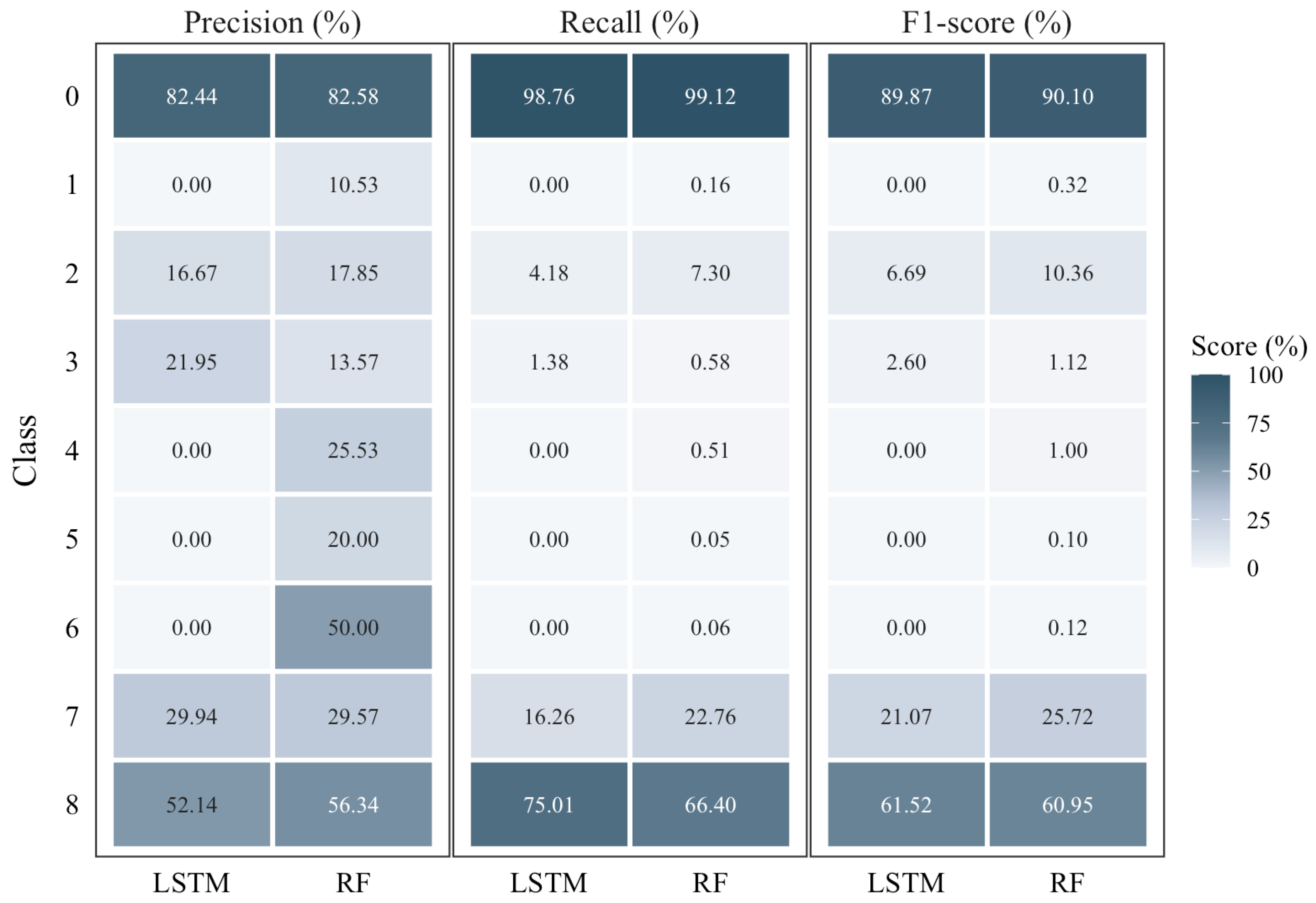
Figure 11 presents the class-wise prediction performance of the LSTM and RF models. Although both models achieve comparable overall accuracy, RF generally provides better performance on the minority queue waiting-time classes. In particular, RF achieves higher precision, recall, and F1-scores for most minority classes, including Classes 1, 2, 4, 5, and 6. In contrast, the LSTM model fails to correctly identify instances from several minority classes (Classes 1, 4, 5, and 6), resulting in zero scores. LSTM performs slightly better for Class 3, achieving higher precision and F1-score than RF; however, the overall performance on this class remains low for both models due to the very low recall.

Figure 11. Class-wise performance comparison between LSTM (Lag-3) and RF (without Lag).

Under the observable historical waiting-time sequence construction evaluated in this study, the LSTM models did not outperform the feature-based RF model. In particular, RF without lag features achieved higher Macro Precision (34.00%) and Macro F1-score (21.09%) than the best-performing LSTM configuration (22.57% and 20.19%, respectively). However, requiring historical waiting times to be observable at the target job’s submission time alters the waiting-time distribution by disproportionately excluding long-waiting jobs. Therefore, the observed results are specific to the sequence construction evaluated in this study and should not be interpreted as evidence that sequence modeling is generally ineffective for queue waiting-time prediction.

4.4. Time-Series Applicability Analysis

We further investigated the applicability of conventional time-series models that rely solely on historical waiting-time observations without incorporating the proposed job submission and queue-state features. We first examined time-series modeling at the individual-job level, where each observation represents one submitted job and its queue waiting time. Jobs were ordered chronologically according to their submission times. For each newly submitted job, only the waiting times of earlier submitted jobs that had already started were known and could therefore be used as historical observations. Earlier jobs that were still waiting in the queue could not be included because their final waiting times were not yet known. This filtering disproportionately removed long-waiting jobs and produced a highly imbalanced time-series dataset. Of the retained observations, 290,770 (99.82%) belonged to Class 0 (≤1 h), while only 373 and 119 observations belonged to Class 1 (≤2 h) and Class 2 (≤4 h), respectively. Only a very small number of observations remained in the higher waiting-time classes. Therefore, the resulting sequence did not adequately represent the original waiting-time distribution, particularly for long-waiting jobs, limiting the applicability of conventional time-series models to individual-job waiting-time prediction. This limitation is particularly relevant because accurate prediction of long-waiting jobs is important for identifying severe queue delays.

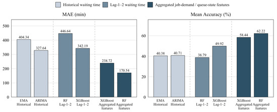
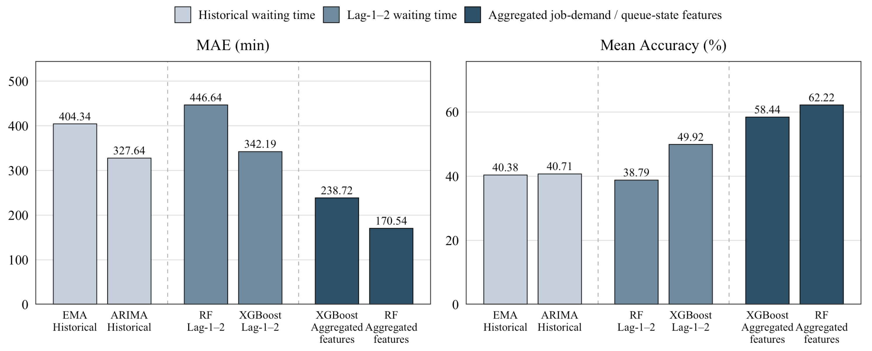
To provide an alternative time-series evaluation, we constructed a daily aggregated dataset. Jobs were ordered by submission time and grouped by submission date. The daily mean queue waiting time was used as the prediction target, while job-demand and queue-state information were aggregated into daily features. For the non-feature-based time-series evaluation, we employed Exponential Moving Average (EMA) and Autoregressive Integrated Moving Average (ARIMA). EMA predicts future waiting times by assigning greater importance to recent historical observations, while ARIMA models temporal dependencies in the historical waiting time sequence using autoregressive, differencing, and moving-average components. Both models rely only on historical daily mean waiting times and do not use the proposed job submission and queue-state features. For comparison, RF and XGBoost regressors were trained using the aggregated daily job-demand and queue-state features. The last 60 days were used as the common hold-out test period for all models.

The prediction performance was evaluated using mean absolute error (MAE) and mean prediction accuracy [14]. MAE is defined as

$$\mathrm{MAE}={\displaystyle \frac{1}{N}}{\displaystyle \sum _{i=1}^N}\left|y_i-{\widehat{y}}_i\right|,$$

(12)

where $y_i$ and ${\widehat{y}}_i$ denote the actual and predicted queue waiting times, respectively. Lower MAE indicates better performance.

The prediction accuracy for each observation is calculated as

$$A_i={\displaystyle \frac{\min (y_i,{\widehat{y}}_i)}{\max (y_i,{\widehat{y}}_i)}},$$

(13)

and the mean prediction accuracy is

$$\mathrm{Mean} \mathrm{Accuracy}={\displaystyle \frac{1}{N}}{\displaystyle \sum _{i=1}^N}{A}_i\times 100\%.$$

(14)

A higher mean accuracy indicates better prediction performance.

To separate the effect of the prediction model from that of the available input information, an additional controlled experiment was conducted in which the RF and XGBoost regressors were restricted to historical daily mean waiting-time information only. Specifically, the two most recent daily mean waiting times (Lag-1 and Lag-2) were used as input features. The same final 60-day period was retained as the hold-out test set. During the hold-out period, predictions were generated recursively so that actual waiting-time observations within the test period were not used as lag inputs.

Figure 12 illustrates the controlled comparison. When restricted to historical waiting-time information, RF and XGBoost did not consistently outperform ARIMA. In contrast, both regressors achieved substantially lower MAE and higher mean prediction accuracy when provided with the aggregated job-demand and queue-state features. RF achieved the best overall performance, with an MAE of 170.54 min and a mean prediction accuracy of 62.22%. These results indicate that the additional job-demand and queue-state information is an important contributor to prediction performance, rather than the observed improvement being explained solely by the choice of RF or XGBoost.

Figure 12. Daily mean queue waiting-time prediction results using the aggregated feature-based RF and XGBoost models compared with EMA and ARIMA.

5. Conclusions and Future Work

In this study, a log-based feature engineering method was proposed for predicting queue waiting time in batch job schedulers of HPC systems, utilizing information available at the time of job submission. Unlike existing studies, which have relied predominantly on static job characteristics at submission time and have shown limitations in adequately capturing the dynamic congestion state of the scheduling system, prediction performance was improved in this study through a range of feature engineering techniques, including the removal of redundant features via Pearson correlation coefficient, Cramér’s V, and mapping consistency analysis, the generation of temporal features capturing periodic submission patterns from the job submission timestamp, and the reconstruction of global and local waiting and running states at the time of job submission. The effectiveness of the proposed approach was validated using large-scale job log data collected from the Theta supercomputer at the ALCF. A comparison of multiple machine learning models, including NB, KNN, RF, and XGBoost, confirmed that the Random Forest model achieved the highest performance, with an accuracy of 88.89%, a balanced accuracy of 57.65%, a macro precision of 67.95%, and a macro F1-score of 61.71%.

This study is significant in that it proposes a feature engineering framework capable of meaningfully improving queue waiting time prediction performance using only information available at the time of job submission. Nevertheless, several limitations remain. Although substantial improvements were achieved relative to the baseline and the reference study, the overall balanced accuracy and macro F1-score remain at moderate levels, at 57.65% and 61.71%, respectively. In particular, prediction performance for the intermediate waiting-time classes (Classes 4–6) remains comparatively low, indicating that further improvement is required before the proposed approach can be considered reliable for practical deployment in operational environments. In addition, the proposed method was validated on a single HPC system (Theta), and its generalizability to systems with different scales, scheduling policies, or workload characteristics has not yet been established.

The sequence-modeling experiment is also limited by the construction of the observable historical waiting-time sequences, which alters the waiting-time distribution by disproportionately excluding long-waiting jobs. Therefore, the sequence-modeling results are specific to the sequence construction evaluated in this study and should not be generalized to sequence models in general.

In addition, the waiting-time class boundaries used in this study were adopted from [3] to maintain consistency with prior work. Although the ordinal-error analysis considers the magnitude of misclassification errors and the regression experiment provides a continuous-target baseline, the sensitivity of the results to alternative class-boundary definitions was not systematically evaluated. Alternative class definitions may change the class distribution and consequently affect model performance.

Future work will therefore focus on verifying the generalization performance of the proposed method across different HPC systems and diverse scheduling policies, as well as further improving prediction performance for minority waiting-time classes, evaluating robustness under alternative waiting-time class definitions.

References

- Qian, J.; Srisa-An, W.; Seth, S.; Jiang, H.; Li, D.; Yi, P. Exploiting FIFO scheduler to improve parallel garbage collection performance. In Proceedings of the 12th ACM SIGPLAN/SIGOPS International Conference on Virtual Execution Environments (VEE’16), Atlanta, GA, USA, 2–3 April 2016; pp. 109–121. [Google Scholar] [CrossRef] [Scilit]
- Yao, Y.; Zhou, N.; Yao, S.; Liang, X.; Deng, W.; Yang, C.; Gui, W. Fairness-aware deterministic joint offloading and scheduling for industrial edge computing. IEEE Trans. Ind. Inform. 2026, 22, 4032–4043. [Google Scholar] [CrossRef] [Scilit]
- Okafor, N.; Lusch, B.; Vishwanath, V. Queue wait time prediction in high performance computing (HPC) systems. J. Supercomput. 2026, 82, 90. [Google Scholar] [CrossRef] [Scilit]
- Park, J.W.; Kwon, M.W.; Hong, T. Queue congestion prediction for large-scale high performance computing systems using a hidden Markov model. J. Supercomput. 2022, 78, 12202–12223. [Google Scholar] [CrossRef] [Scilit]
- Brown, N.; Gibb, G.; Belikov, E.; Nash, R. Predicting accurate batch queue wait times on production supercomputers by combining machine learning techniques. Concurr. Comput. Pract. Exp. 2024, 36, e8112. [Google Scholar] [CrossRef] [Scilit]
- Chen, T.; Guestrin, C. XGBoost: A Scalable Tree Boosting System. In Proceedings of the 22nd ACM SIGKDD International Conference on Knowledge Discovery and Data Mining (KDD ’16), San Francisco, CA, USA, 13–17 August 2016; pp. 785–794. [Google Scholar] [CrossRef] [Scilit]
- Kumar, R.; Vadhiyar, S. Identifying quick starters: Towards an integrated framework for efficient predictions of queue waiting times of batch parallel jobs. In Proceedings of the 16th Workshop on Job Scheduling Strategies for Parallel Processing (JSSPP’12), Held in Conjunction with IPDPS 2012, Shanghai, China, 25 May 2012; pp. 196–215. [Google Scholar] [CrossRef] [Scilit] [PubMed]
- Vercellino, C.; Scionti, A.; Varavallo, G.; Viviani, P.; Vitali, G.; Terzo, O. A machine learning approach for an HPC use case: The jobs queuing time prediction. Future Gener. Comput. Syst. 2023, 143, 215–230. [Google Scholar] [CrossRef] [Scilit]
- Kumar, R.; Vadhiyar, S. Prediction of queue waiting times for metascheduling on parallel batch systems. In Proceedings of the 18th Workshop on Job Scheduling Strategies for Parallel Processing (JSSPP’14), Held in Conjunction with IPDPS 2014, Phoenix, AZ, USA, 23 May 2014; pp. 108–128. [Google Scholar] [CrossRef] [Scilit]
- Downey, A.B. Predicting queue times on space-sharing parallel computers. In Proceedings of the 11th International Parallel Processing Symposium (IPPS’97), Geneva, Switzerland, 1–5 April 1997; pp. 209–218. [Google Scholar] [CrossRef] [Scilit]
- Downey, A.B. Using queue time predictions for processor allocation. In Proceedings of the 3rd Workshop on Job Scheduling Strategies for Parallel Processing (JSSPP’97), Held in Conjunction with IPPS’97, Geneva, Switzerland, 5 April 1997; pp. 35–57. [Google Scholar] [CrossRef] [Scilit] [PubMed]
- Smith, W.; Taylor, V.; Foster, I. Using run-time predictions to estimate queue wait times and improve scheduler performance. In Proceedings of the 5th Workshop on Job Scheduling Strategies for Parallel Processing (JSSPP’99), Held in Conjunction with IPPS/SPDP’99, San Juan, PR, USA, 16 April 1999; pp. 202–219. [Google Scholar] [CrossRef] [Scilit] [PubMed]
- Nurmi, D.C.; Brevik, J.; Wolski, R. QBETS: Queue bounds estimation from time series. ACM SIGMETRICS Perform. Eval. Rev. 2007, 35, 379–380. [Google Scholar] [CrossRef] [Scilit]
- Sonmez, O.; Yigitbasi, N.; Iosup, A.; Epema, D. Trace-based evaluation of job runtime and queue wait time predictions in grids. In Proceedings of the 18th ACM International Symposium on High Performance Distributed Computing (HPDC’09), Garching, Germany, 11–13 June 2009; pp. 111–120. [Google Scholar] [CrossRef] [Scilit]
- Gaikwad, B.; Simakov, N.A.; Furlani, T.; White, J.P.; Patra, A. Predictive modeling of HPC job queue times: Improving user decision-making and resource utilization. In Proceedings of the Practice and Experience in Advanced Research Computing 2025: The Power of Collaboration (PEARC’25), Columbus, OH, USA, 20–24 July 2025; pp. 1–4. [Google Scholar] [CrossRef] [Scilit]
- Lovell, A.; Wisniewski, P.; Rodenbeck, S.; Ashish. A hierarchical deep learning approach for predicting job queue times in HPC systems. In Proceedings of the SC24-W: Workshops of the International Conference for High Performance Computing, Networking, Storage and Analysis, Atlanta, GA, USA, 17–22 November 2024; pp. 621–628. [Google Scholar] [CrossRef] [Scilit]
- Argonne Leadership Computing Facility. ALCF Public Data. 2026. Available online: https://reports.alcf.anl.gov/data/ (accessed on 14 August 2026).
- Cramér, H. Mathematical Methods of Statistics; Princeton University Press: Princeton, NJ, USA, 1946. [Google Scholar]
- Fenwick, P.M. A new data structure for cumulative frequency tables. Softw. Pract. Exp. 1994, 24, 327–336. [Google Scholar] [CrossRef] [Scilit]
- Yoo, A.B.; Jette, M.A.; Grondona, M. SLURM: Simple Linux Utility for Resource Management. In Proceedings of the Job Scheduling Strategies for Parallel Processing: 9th International Workshop, JSSPP 2003, Seattle, WA, USA, 24 June 2003; Revised Paper; Lecture Notes in Computer Science; Feitelson, D., Rudolph, L., Schwiegelshohn, U., Eds.; Springer: Berlin/Heidelberg, Germany, 2003; Volume 2862, pp. 44–60. [Google Scholar] [CrossRef] [Scilit]
Disclaimer/Publisher’s Note: The statements, opinions and data contained in all publications are solely those of the individual author(s) and contributor(s) and not of MDPI and/or the editor(s). MDPI and/or the editor(s) disclaim responsibility for any injury to people or property resulting from any ideas, methods, instructions or products referred to in the content. |
© 2026 by the authors. Licensee MDPI, Basel, Switzerland. This article is an open access article distributed under the terms and conditions of the Creative Commons Attribution (CC BY) license.