


Abstract
To reveal the full-process characteristics of landslide stability with deformation evolution, this paper proposes a novel progressive failure stability analysis method based on the improved slice method. By analyzing the force distribution characteristics of thrust-type and traction-type landslides along the sliding surface, the dynamic evolution laws of the unstable zone, critical state zone, and stable zone on the sliding surface are clarified. Based on the stress–strain discontinuity of the sliding surface, parameters such as failure rate, failure area ratio, and friction resistance variation coefficient are introduced to construct a point–surface–body multi-dimensional stability evaluation index system, including Comprehensive Shear Resistance Method (CSRM), Comprehensive Displacement Method (CDM), Surplus Displacement Method (SDM), and Main Thrust–Main Tension Method (MTM). A new unbalanced thrust method is derived to realize the quantitative simulation of the whole progressive failure process of landslides. The Kaziwan large bedrock landslide is taken as an example for verification. The results show that the critical state slice (slice No. 29) determined by the new method is completely consistent with the investigation results; the calculated displacements are in good agreement with the measured values of multiple inclinometers; the four stability coefficients show regular attenuation with the forward movement of critical slices, which can effectively describe the catastrophe process of landslides from local initiation to overall penetration. This method provides reliable support for dynamic stability evaluation and catastrophe mechanism research of landslides.
1. Introduction
Landslides represent one of the most widespread and destructive geological hazards worldwide, affecting mountainous regions under the combined influences of tectonic activity, extreme precipitation, climate variability, and human disturbance [1]. According to global landslide inventories, more than 90% of rainfall- and earthquake-induced landslides occur in developing countries, with Asia accounting for the largest proportion of reported landslide events due to its extensive mountainous terrain and intense monsoon activity. The Himalayan–Tibetan orogenic belt, the most tectonically active region in the world, together with densely populated mountainous areas in China, Nepal, India, and Southeast Asia, constitutes one of the global hotspots of landslide disasters. Previous studies have indicated that thousands of fatalities and substantial economic losses occur annually worldwide due to landslides, while Asia contributes a dominant share of both landslide occurrence and associated casualties [2,3].
China is particularly vulnerable to landslide hazards because approximately 69% of its territory consists of mountainous and plateau regions, where active tectonics, complex geological structures, steep terrain gradients, and intensive rainfall events frequently trigger slope instability [4]. Historical records show that large-scale landslide disasters in southwestern China have caused considerable casualties and economic impacts, highlighting the urgent need for reliable stability assessment and failure prediction methods for complex slopes [4,5].
Many scholars have conducted long-term research on slope engineering. On the premise of the assumption that all points along the sliding surface are in a critical state, slope stability analysis methods, including limit equilibrium approaches and strength reduction techniques, have been widely developed, and the movement modes of slopes after overall failure and instability have been classified. The ratio of frictional resistance (or stress) to downslope driving force (or stress) at the critical state of the sliding surface is defined as the safety factor (or stability factor). The basic characteristics of the existing methods are as follows: the reduction factor is taken as the overall stability index of the slope; the stability factor in the slice method is independent of deformation; the numerical calculation of strength reduction mostly adopts an ideal elastoplastic constitutive model and assumes stress–strain continuity, and local strength reduction is carried out under constant boundary conditions. Moreover, a sufficient comparative analysis between numerical results and slice method results is still lacking. Nevertheless, collapse accidents still occur frequently in practical engineering applications when adopting these traditional methods [6,7,8,9,10].
In fact, there are significant differences in displacement and stress distribution at different positions during landslide failure. Landslide stability is closely related to parameters such as displacement and stress. The entire evolutionary mechanism of landslides, from local initiation and sliding surface expansion, connection and penetration to overall instability, is all associated with displacement. Traditional landslide stability analysis theories generally adopt global safety factors and critical state assumptions, which may not fully describe progressive failure evolution, fail to consider the progressive evolution process of catastrophic failure, and lack a constitutive model that can describe the full failure process of rock and soil mass. Essentially, catastrophic landslide failure is a progressive damage process involving stress redistribution, deformation accumulation, strength degradation, and sliding surface propagation [9,10,11,12,13].
Existing studies have the following major limitations. The description and quantification of landslide stability merely depend on the overall stability factor, lacking dynamic interpretation of the whole evolutionary process of failure [14]. Most current investigations on failure mechanisms focus on shear–compression failure and adopt strength criteria for judgment. Few studies have involved the process description and analysis of point-by-point propagation (forward or backward migration) of the landslide sliding surface [15,16]. The failure process is closely related to boundary conditions and geological features, which can trigger composite failure modes such as compression–shear, tension, and tension–shear failure. There is insufficient analysis on the disaster-forming mechanism of parameters including failure area, pressure, thrust force, and frictional resistance, as well as the corresponding deformation during landslide progressive failure. No existing research has revealed the stress–displacement discontinuity characteristics within the progressive failure zone of landslides [17]. Moreover, landslide stability evaluation adopts a single index that only relies on the stability coefficient, without systematic characterization of multi-parameter evolution throughout the entire failure process.
In summary, it is of great necessity to construct a point–surface–volume multi-parameter evaluation system that can characterize the progressive failure process of slope stability and establish a constitutive model covering the entire failure process of rock and soil mass. This work is essential for the comprehensive stability assessment of landslides considering full-cycle progressive failure characteristics. In addition, the theoretical assumptions and engineering limitations of the proposed indices are explicitly discussed to clarify their applicability in practical landslide assessment.
To address the above limitations, this study aims to establish a progressive failure stability evaluation framework for landslides by coupling an improved slice method with a shear stress–strain constitutive model. The main objectives are: (1) to characterize the spatial evolution of unstable, critical, sub-stable and stable zones along the sliding surface; (2) to develop a multi-parameter stability evaluation system considering stress failure rate, strain failure rate, failure area ratio, displacement evolution and frictional resistance variation; and (3) to quantitatively describe the whole process of landslide instability from local failure initiation to complete sliding surface penetration.
The scientific novelty of this study lies in shifting landslide stability evaluation from a single global safety factor toward a progressive, deformation-related and multi-parameter description. Unlike conventional limit equilibrium or strength reduction methods, which usually assume that the sliding surface reaches a critical state simultaneously, the proposed framework considers the non-uniform stress–strain state and discontinuous deformation evolution along the sliding surface. The main contributions of this work are as follows: first, a point–surface–body multi-dimensional stability index system is constructed; second, a new unbalanced thrust calculation procedure is derived to track the migration of the critical state slice; third, four complementary stability coefficients, namely CSRM, CDM, SDM, and MTM, are introduced to evaluate progressive failure from different mechanical perspectives; and finally, the proposed method is validated using the Kaziwan landslide case, demonstrating its ability to capture the evolution of landslide instability more explicitly than traditional stability analysis methods.
The remainder of this paper is organized as follows. Section 2 introduces the failure modes of thrust-type and retrogressive landslides and analyzes the stress–strain evolution characteristics along the sliding surface. Section 3 establishes the two-dimensional stability analysis framework for landslide progressive failure, including the description of stability states, force distribution characteristics, slice division procedure, and multi-parameter stability indices. Section 4 presents the shear stress–strain constitutive model and the improved unbalanced thrust calculation method for simulating the progressive failure process. Section 5 applies the proposed framework to the Kaziwan landslide and describes the engineering geological conditions, calculation model, and parameter determination. Presents and discusses the stability evaluation results, critical state evolution, and displacement verification. Finally, Section 6 summarizes the main conclusions, discusses the limitations of the proposed method, and outlines future research directions.
2. Failure Modes of Slopes
2.1. Thrust-Type Landslide
Landslide stability is closely related to the mechanical properties of local points on the sliding surface, where stress–strain evolution and strength degradation characteristics control failure development. The full shear load–displacement curves of rock and soil masses exhibit Type I and Type III characteristics (Figure 1) [18]. The stress–strain evolution of a single point on the sliding surface sequentially undergoes elastic, elastoplastic, peak failure, and residual stages. Points and correspond to the stress state points in the post-failure zone, and point is defined as the critical state point. Points and represent the transitional stress states between the peak stress and the elastic limit stress of the sliding mass, and point represents the elastic limit stress state. These state points represent four typical stress conditions: post-failure stress, peak stress, elastoplastic stress, and elastic stress. The sliding mass may fail along the weak sliding surface , along the weak sliding surface , or within the front-edge sliding mass . The failure modes of geotechnical materials are significantly controlled by shear stress–strain behavior [19].
Figure 1.
Shear stress–shear strain diagram of thrust-type landslide.
2.2. Retrogressive Landslide
In the two-dimensional retrogressive landslide shown in Figure 2, points and represent the stress state points in the post-failure zone, point represents the peak stress state point, and points can represent elastoplastic or elastic stress state points. These stress state points correspond to four stability states, namely unstable, critical, sub-stable, and stable. Among them, point is the peak stress state point, while points and have already undergone the peak stress stage. The landslide failure modes include failure along the weak sliding surface (), Type II failure where the front edge fails along the weak sliding surface and the rear edge fails within the sliding mass , as well as Type III failure caused by tensile failure of the sliding mass ).
Figure 2.
Shear stress–shear strain diagram of retrogressive landslide.
3. Two-Dimensional Stability Analysis of Landslides
3.1. Description of State and Variation
During the evolution process of deformation and failure of a landslide mass, its stability gradually attenuates until eventual instability and failure. To further interpret this evolutionary process, several key concepts are established to characterize the mechanical response and state evolution of the landslide mass.
The failure of a landslide originates in local areas and expands progressively. When the driving shear stress at a certain point of the sliding mass exceeds its shear strength, failure occurs at that point. The downslope force at the rear edge of the sliding mass is generally greater than the anti-sliding force, causing this area to first enter a failure state (unstable zone) or a critical failure state (sub-stable zone). The boundary between the two states is the critical state when the driving stress reaches the ultimate strength of the geomaterial. It is worth noting that the critical state does not necessarily correspond to the peak stress. For instance, the stress corresponding to the critical state can be a specific stress state. After the landslide undergoes overall failure and tends to be stable following movement, secondary failure may occur in the rear edge region. This indicates that the critical state and mechanical critical value may present coupled or deviated mechanical characteristics. By contrast, the front edge of the sliding mass is usually in a stable state (stable zone) due to its relatively small downslope force.
With temporal evolution, mechanical parameters of the landslide mass, including anti-sliding force, driving force, tangential displacement, normal displacement, and normal pressure, change dynamically. To quantitatively characterize such evolutionary processes, variation coefficients of each parameter are introduced. Among them, the variation coefficient of frictional resistance is defined as the ratio of the current vector sum of frictional resistance to its initial vector sum; the variation coefficient of driving force is defined as the ratio of the current vector sum of driving force to its initial value. These coefficients can effectively reflect the transformation of mechanical characteristics of the landslide mass at different evolutionary stages.
3.2. Characteristics of Force Distribution
When the slope undergoes progressive deformation and failure, the generation mechanism of sliding surface displacement originates from the downward stresses () applied above the sliding block. While the sliding surface stresses act on the sliding bed, the sliding bed exerts opposite stresses () on the sliding surface elements beneath the sliding surface (as shown in Figure 3). Among them, the downslope force at the rear edge of the sliding surface is generally greater than the anti-sliding force. In the critical state, the downslope force equals the anti-sliding force and the anti-sliding force reaches its peak value. At the front edge of the sliding surface, the downslope force equals the anti-sliding force, which is less than the critical value. Figure 4 is a schematic diagram of forces acting on a two-dimensional thrust-type landslide, where Pi and Ni represent the downslope force and pressure of the sliding mass, respectively, and Fi and represent the frictional resistance and counter pressure of the sliding bed. The frictional resistance Nm at the critical point is the critical value. The upper region becomes an unstable zone because the downslope force of the sliding surface is greater than the frictional resistance, while the lower region forms a stable zone because the downslope force equals the frictional resistance. Force analysis shows that the sliding mass is in a non-equilibrium state during progressive deformation and failure: the downslope force is always greater than or equal to the frictional resistance, and the normal pressure equals the counter pressure, with the frictional resistance at the critical point reaching the maximum value.
Figure 3.
Stress distribution diagram of sliding surface element.
Figure 4.
Force distribution diagram of thrust-type landslide.
When the landslide mass reaches the critical stress state, the stress evolves gradually until the last slice (or element) exhibits a critical mechanical response, thereby revealing the stress–strain distribution characteristics of the sliding surface. The stresses and strains at this moment are defined as the normal stress at failure (), frictional shear stress at failure (), shear strain at failure (), and driving downslope stress at failure ().
3.3. Description of Stability
3.3.1. Slice Description
In the slice method, the slope mass is divided into discrete slices to satisfy equilibrium conditions, which forms the basis of classical slope stability analysis [20,21,22]. Taking a trapezoidal slice as an example, assume that the coordinates of the four vertices of the m-th trapezoidal slice are , , , and in sequence, and the inclination angle of the slice is . If there exists an unbalanced thrust force from the (m − 1)-th slice, the original m-th slice is re-divided into the m-th and (m + 1)-th slices. Point constitutes the re-divided m-th slice (as shown in Figure 5 and Figure 6). The method for solving the coordinates of point is as follows:
Figure 5.
Coordinate diagram of slice division.
Figure 6.
Schematic diagram of slice division.
The equations of the straight lines formed by points and are as follows:
It can be seen from this that points and represent the point coordinates and . The side length lm and weight Wm of trapezoid can be calculated based on the coordinates. Therefore, there is only one unknown variable in the above equations.
3.3.2. Stability Description of Sliding Surface Points
The stress failure rate is defined as the ratio of the driving shear stress to its peak shear stress. When this ratio is greater than 1, the point is judged to have undergone stress failure, and the value is set to 1. If the ratio is less than 1, it represents the corresponding possibility of stress failure at that point. The strain failure rate can also be described using a similar definition.
In the formula, and represent the driving shear stress and strain of the sliding surface point in the i direction, respectively. Correspondingly, and represent the peak shear stress and strain in the i direction, respectively.
3.3.3. Stability Description of Sliding Surface
The stress failure area ratio of the entire sliding surface is defined as the ratio of the sum of the areas of slices before the critical state to the total area of all slices during the propagation of the landslide mass along the potential failure surface, which is used to characterize the proportion of the area in the failure state. When is greater than or equal to 1, it indicates that stress failure has occurred along the entire sliding surface. When the ratio is less than 1, it reflects the possibility of impending stress failure of the landslide along the sliding surface. The expressions of the stress failure area ratio in the X direction, Y direction, and the resultant vector direction are as follows:
Similarly, the strain failure area ratios (, , ) in the X direction, Y direction, and the resultant vector direction can be defined.
The frictional resistance variation coefficient is defined as the ratio of the current frictional resistance vector sum to the reference frictional resistance vector sum. The expressions of the variation coefficients along the X direction, Y direction, and the resultant vector direction are as follows:
The driving downslope force variation coefficient is defined as the ratio of the current driving downslope force vector sum to the initial driving downslope force vector sum. The expressions of the variation coefficients along the X-axis, Y-axis, and the resultant vector direction are as follows:
The normal pressure variation coefficient is defined as the ratio of the current normal pressure vector sum to the reference normal pressure vector sum. The expressions of the variation coefficients along the X-axis, Y-axis, and the resultant vector direction are as follows:
The tangential displacement variation coefficient is defined as the ratio of the current tangential displacement vector sum to the reference tangential displacement vector sum. The expressions of the variation coefficients along the X-axis, Y-axis, and the resultant vector direction are as follows:
The coefficients defined by the above formulas all encompass the X and Y directional components and vector characteristics. Slices 1 to m are in the post-failure zone state, while slices m + 1 to n are in the pre-peak state.
In the above expressions:
—Inclination angle of the slice;
m—Number of slices in critical stress state;
li—Base length of the slice sliding surface;
—Current shear strain;
n—Total number of slices;
—Current driving shear stress;
—Current frictional resistance stress;
—Current normal stress.
4. Description of Progressive Failure of Landslides
4.1. Stress and Strain Distribution of Sliding Surface by Shear Stress Model
To quantitatively describe the progressive failure characteristics of slopes, basic equations for slices are established based on the proposed shear stress model and the shear stress–shear strain relationship curve in Figure 7 [23].
Figure 7.
Constitutive model curve.
This constitutive model (Equation (22)) can uniformly describe three types of mechanical behavior of geotechnical materials: strain softening, strain hardening, and ideal plasticity [24,25,26]. When the parameter combination satisfies condition , the model exhibits strain softening characteristics: the shear stress rises to a peak value first and then decreases to the residual value with increasing shear strain. This mode is suitable for describing the progressive failure process of softening materials such as loess and structural clay. When condition is satisfied, the model presents strain hardening characteristics and is applicable to hardening materials such as dense sand. When condition is satisfied, the model degenerates into an ideal elastoplastic model. By adjusting the values of and , the model can continuously characterize the transition behavior from brittle to ductile.
In this equation, is the initial shear modulus of the i-th slice (with the same dimension as stress), denotes the shear strain (dimensionless), and are dimensionless model parameters, and is a dimensionless material constant. controls the steepness of the post-peak stress drop for the i-th slice: a larger leads to a sharper post-peak decline and higher material brittleness, while a smaller results in a more gradual post-peak degradation. , together with and , governs the morphological characteristics of the post-peak softening segment and affects the magnitude of critical strain via Equation (23), with its value calibrated by fitting the stress–strain curves from ring shear tests. Parameter regulates the rate of post-peak stress drop: the closer is to 0, the slower the post-peak stress decreases and the stronger the material ductility; the closer is to −1, the steeper the post-peak stress drops and the stronger the material brittleness. The value of is adopted in this study, and the rationality of this constraint is reflected in three aspects: mathematically, when condition is satisfied, Equation (22) may exhibit singularity or non-physical divergence under condition , failing to ensure the asymptotic behavior that shear stress approaches the residual value as strain increases infinitely; physically, the above value range exactly covers the complete response spectrum from highly brittle behavior to near-ideal plasticity ; and in terms of experimental calibration, according to the fitting results of ring shear test curves for various soil types in this work, the value of generally ranges from −0.99 to −0.3, and the constraint of covers all measured cases.
The critical strain space satisfies the following expression:
In the formula: —Critical strain corresponding to the critical stress
In the formula:
—Normal stress;
—Cohesion, where the units of and are Pa, kPa, or MPa;
—Friction angle of the sliding surface.
In the formula: —Constant coefficient.
In the formula:
—Value of under the corresponding condition;
and are constant coefficients;
is a dimensionless parameter;
has the dimension of Pa−1, kPa−1 or MPa−1.
For parameter , it can be expressed with reference to the reference soil-water characteristic curve as follows:
In the formula:
—Value of ρi when the normal stress is zero;
—Value of ρi under any normal stress when equals ;
—Parameter of the constant coefficient equation (which can be determined by solving the stresses obtained from shear tests).
4.2. New Unbalanced Thrust Method
The basic assumptions are as follows: (1) the slices are assumed to be elastic and are divided at vertical intervals; (2) the force exerted by the (i + 1)-th slice on the i-th slice is parallel to the base of the (i + 1)-th slice and acts at the geometric center of the i-th slice; (3) the shear interaction between adjacent slices is neglected; (4) the rotational effect of the slices is not considered; (5) the anti-sliding force at the base of each slice satisfies the corresponding constitutive equation; and (6) the strain of the i-th slice along the landslide base is approximately equal to the vector sum of the strains of the (i + 1)-th slice in the directions parallel and perpendicular to the base, as shown in Figure 8.
Figure 8.
Strain relationship between adjacent slices.
The solution procedures for the stress state and strain state along the sliding surface are as follows:
This expression can be simplified as follows:
The expression for normal stress is as follows:
The expression for frictional stress is as follows:
The expression for anti-sliding frictional resistance is as follows:
The expression for critical frictional stress is as follows:
The expression for critical frictional resistance is as follows:
The expression for driving sliding force is as follows:
The expression for driving shear stress is as follows:
The expression for residual sliding force is as follows:
The expression for unbalanced thrust is as follows:
In the above expressions:
, and —Weight, base shear strain and normal stress of the slice, respectively;
and —Horizontal and vertical uniformly distributed loads;
—Base length of the slice;
—Angle between the slice base and the horizontal plane;
and —Corresponding friction angle and cohesion parameters..
When the m-th slice is in the critical state, the unbalanced thrust of the m-th slice shall be set to zero, and the unbalanced thrust exerted by the (m − 1)-th slice on the m-th slice is .
Under the failure mode of the shear stress model, if the calculation determines that the (m + 1)-th slice is in the peak stress state, the displacement of the failed slice shall be increased (taking the displacement of the 1st slice of the landslide as an example). As the shear strain continues to increase, the frictional stress shows a decreasing trend. When the calculation proceeds to the m-th slice, it is common that the unbalanced thrust of the m-th slice is not zero.
At this point, it is necessary to calculate the unbalanced thrust exerted by the m-th slice on the (m + 1)-th slice. Based on the obtained unbalanced thrust , the new normal stress, peak frictional stress, and peak shear strain of the (m + 1)-th slice of the landslide are further calculated. In addition, the same method as above is applied to the (m + 2)-th to n-th slices of the landslide until the unbalanced thrust of the final n-th slice is zero. The finally calculated stress and strain values are the stress and strain at the time of landslide failure, denoted, respectively, as failure driving sliding stress , failure frictional shear stress , failure shear strain , and failure normal stress .
4.3. Landslide Stability Evaluation Method
The stability evaluation methods developed in this section are established on the basis of classical limit equilibrium theory, slice-based slope stability analysis, progressive failure theory, and deformation-dependent shear constitutive descriptions [27,28,29]. Conventional slice methods, such as the Bishop, Morgenstern–Price, and Spencer methods, provide the mechanical basis for decomposing the landslide body into slices and evaluating the balance between driving and resisting forces. However, these methods generally adopt a global safety factor and usually assume that the potential sliding surface reaches a critical state simultaneously. Progressive failure studies have shown that the mobilized shear strength and displacement along a sliding surface are spatially non-uniform, and that failure may propagate gradually from a local zone to the whole sliding surface. Therefore, the present study extends the conventional force-based evaluation into a multi-parameter framework by incorporating stress, strain, displacement, and failure-propagation characteristics [30,31].
It should be emphasized that the proposed indices are not intended to replace classical limit equilibrium or numerical methods in all engineering situations. Instead, they provide complementary indicators for describing the progressive failure process under the assumptions of a predefined sliding surface, two-dimensional analysis, and shear stress–strain parameters obtained from tests or back analysis. The theoretical basis, applicable conditions, and limitations of each index are discussed below.
4.3.1. Comprehensive Sliding Force–Anti-Sliding Force Stability Coefficient (CSRM)
The Comprehensive Sliding Force–Anti-Sliding Force Method (CSRM) is conceptually derived from the classical limit equilibrium definition of the safety factor, in which slope stability is evaluated by the ratio between resisting forces and driving forces along a potential sliding surface. In contrast to conventional slice methods that commonly use a single global safety factor, CSRM introduces the stress state obtained from the shear stress–strain model and calculates the vector relationship between the current driving shear stress and the mobilized frictional resistance. Thus, CSRM can be regarded as a deformation-dependent extension of the conventional force–equilibrium stability coefficient.
Based on the shear stress–strain model, the current normal stress , driving shear stress , frictional stress , and shear strain are obtained, and the overall stability evaluation index of the landslide mass is expressed as follows:
The components of the residual sliding force of each slice in the X and Y directions are calculated as follows:
is the minimum angle formed between the x-axis and the vector :
The components in the X and Y directions and the resultant vectors of the frictional resistance and normal stress of each slice along the sliding surface in the failure state are as follows:
is the minimum angle formed between the X-axis and the resultant vector T:
The definition of CSRM in the X-axis direction is as follows:
The definition of CSRM in the Y-axis direction is as follows:
The definition of CSRM in the driving force direction is as follows:
The main theoretical limitation of CSRM is that it still inherits the equilibrium assumption of conventional slice methods and therefore cannot independently determine the initiation position or propagation direction of local failure. In practical applications, CSRM is suitable for overall stability evaluation when displacement monitoring data are insufficient, but its reliability depends strongly on the accuracy of the predefined sliding surface, slice division, unit weight, pore-water pressure, and shear strength parameters. Therefore, CSRM should be used together with propagation-based or displacement-based indices when progressive deformation data are available.
4.3.2. Main Thrust–Main Tension Method Stability Coefficient (MTM)
The Main Thrust–Main Tension Method (MTM) is developed from the unbalanced thrust method and the mechanical interpretation of progressive failure propagation in thrust-type and retrogressive landslides. The traditional unbalanced thrust method evaluates the transfer of residual sliding force between adjacent slices and is widely used in landslide stability analysis. However, the conventional formulation mainly focuses on the final equilibrium state and pays limited attention to the migration of the critical slice during progressive failure. In this study, MTM extends the unbalanced thrust concept by vectorially synthesizing the residual sliding forces before and after the critical slice, so that the dominant direction and propagation tendency of landslide failure can be identified.
At present, the main thrust method is commonly used to evaluate the stability of thrust-type landslides: the residual sliding force of each element along the sliding surface from the initial landslide slice (the 1st slice) to the critical slice (the m-th slice) is vectorially synthesized in the X and Y directions, and then the horizontal vector , vertical vector and the minimum angle between the resultant vector and the horizontal axis are obtained, respectively.
is the minimum angle formed between the X-axis and the resultant vector :
From the (m + 1)-th slice to the n-th slice, the components in the X and Y directions and the resultant vectors of the differences between the frictional stress at failure and the current frictional stresses and for each landslide slice along the sliding surface are, respectively, as follows:
is the minimum angle formed between the X-axis and the resultant vector:
MTM in the X-axis direction is as follows:
MTM in the Y-axis direction is as follows:
MTM along the main sliding direction is as follows:
For the stability evaluation of retrogressive landslide masses, the main tension method with a similar definition to the main thrust method can be adopted, and its calculation logic is consistent with that of the main thrust method for thrust-type landslides. The theoretical limitation of MTM is that the method requires a clear judgment of the landslide type and the location of the critical slice. If the failure mechanism changes from a typical thrust-type or retrogressive mode to a compound mode involving tension cracking, lateral spreading, or multi-stage sliding, the interpretation of the main thrust or main tension direction may become uncertain. In engineering practice, MTM is sensitive to the spatial discretization of slices and to the estimation of residual sliding forces between adjacent slices. Therefore, MTM is most suitable for landslides with a relatively clear propagation direction and should be interpreted cautiously for slopes with multiple potential sliding surfaces or strong three-dimensional constraints.
4.3.3. Comprehensive Displacement Method Stability Coefficient (CDM)
The Comprehensive Displacement Method (CDM) is based on the deformation-controlled interpretation of landslide stability. Previous studies on progressive failure and landslide monitoring have indicated that displacement and shear strain are more sensitive than a single safety factor in identifying the transition from local deformation to global instability [32,33]. Therefore, CDM evaluates landslide stability by comparing the current cumulative shear displacement or shear strain state with the displacement state corresponding to failure.
In the X and Y axis directions and the resultant vector direction, the current shear strain of each slice is as follows:
The resultant vector is , and the minimum angle formed between it and the X-axis is :
The failure displacement of each slice in the x-direction, y-direction, and its resultant vector can be defined by similar methods, specifically as follows:
The resultant vector is S, and the minimum angle formed between it and the X-axis is :
CDM in the X-axis direction is as follows:
CDM in the Y-axis direction is as follows:
CDM along the main displacement sliding direction is as follows:
The theoretical advantage of CDM is that it directly reflects deformation evolution, whereas its limitation is that the critical displacement or failure strain must be defined in advance. In practice, this value may vary with lithology, normal stress, water content, shear rate and the degree of previous deformation. CDM is therefore more reliable when laboratory shear tests, inclinometer data or back-analysis results are available. Without sufficient displacement monitoring data, CDM may introduce large uncertainty and should not be used as the only criterion for stability judgment.
4.3.4. Surplus Displacement Method Stability Coefficient (SDM)
The Surplus Displacement Method (SDM) is proposed to quantify the remaining deformation capacity from the current state to the failure state. Its basic idea is consistent with deformation-based early-warning approaches, in which the safety reserve of a landslide is evaluated not only by force equilibrium but also by the residual displacement or strain capacity before failure [34]. Compared with CDM, SDM focuses on the difference between the current displacement state and the critical displacement state, and is therefore more suitable for evaluating the remaining safety margin.
After selecting the sliding mass, the displacement of each unit failing along the sliding surface is calculated within the range of the divided 1st to n-th slices. The displacement vectors in the X and Y directions are summed, respectively, obtaining the displacement vector sums in the X and Y directions as and , and the resultant vector as .
is the minimum angle formed between the x-axis and the resultant vector :
Within the interval of the divided slices from m = 2 to n, when the sliding mass undergoes overall failure along the sliding surface, the difference between the current displacement and the critical displacement of each landslide slice along the sliding surface at that moment needs to be calculated. By vectorially summing the displacement differences in the X and Y directions, respectively, the displacement difference vector sums in the X and Y directions are obtained as and , and the resultant vector is obtained as . Then the minimum angle formed between the resultant vector and the x-axis is calculated as .
The stability coefficient of SDM in the X-axis direction is as follows:
The stability coefficient of SDM in the Y-axis direction is as follows:
The stability coefficient of SDM along the main displacement sliding direction is as follows:
The theoretical limitation of SDM is that the remaining displacement capacity is not a material constant but a state-dependent quantity affected by stress path, hydrological condition, strain-softening behavior, and boundary constraints. In practical applications, SDM requires continuous or repeated displacement monitoring and a reasonable definition of the critical displacement. When monitoring records are short, discontinuous, or affected by construction disturbance and rainfall-induced pore-pressure fluctuation, the calculated surplus displacement may not represent the true remaining deformation capacity. Therefore, SDM is recommended for early-warning analysis only when it is combined with field monitoring, hydrogeological interpretation, and other stability indices.
Based on an in-depth investigation of the landslide failure mechanism, a novel analysis method is constructed by integrating the traditional slice method within the framework of the shear stress model, and a multi-dimensional stability evaluation index system is proposed. Among them, the sliding surface point–surface stability evaluation indices include the stress failure ratio, stress failure rate, and stress–strain variation coefficient; the sliding mass stability evaluation methods cover the landslide comprehensive Sliding Force–Anti-Sliding Force Method (CSRM), landslide Surplus Displacement Method (SDM), landslide Comprehensive Displacement Method (CDM), landslide tensile failure method, and landslide Main Thrust–Main Tension Method (MTM), etc. The flowchart of the comprehensive stability evaluation method for the whole-process progressive failure characteristics of landslides shown in Figure 9 demonstrates that these evaluation approaches comprehensively consider multi-source parameters of the landslide mass such as force field, stress, strain, and displacement from different dimensions, achieving a comprehensive characterization of landslide stability from the point–surface–body multi-dimensional perspective.
Figure 9.
Flowchart of the stability evaluation method for landslide progressive failure characteristics.
4.3.5. Applicable Conditions, Selection Principles, and Limitations of the Four Stability Evaluation Methods
The four stability evaluation methods described above characterize the stability state of landslides from different physical dimensions. Each method has its unique applicable conditions and advantages; they are not redundant but complementary to one another. According to their physical essence, they can be classified into two categories: force-based methods (CSRM and MTM) and displacement-based methods (CDM and SDM). CSRM evaluates the overall stability of landslides from the perspective of global equilibrium, with a physical meaning closest to the traditional safety factor and is suitable for basic evaluation when monitoring data are unavailable. MTM is specifically developed for thrust-type/retrogressive landslides and can describe the propagation process of failure from the trailing edge to the toe (or vice versa). CDM directly adopts field displacement monitoring data and is applicable to the validation of landslides with inclinometer records. SDM provides information on the safety margin from the current state to displacement failure, which is appropriate for the determination of early warning thresholds. The applicable conditions and unique advantages of the four methods are summarized in Table 1.
Table 1.
Theoretical Basis, Applicable Conditions, Advantages, and Limitations of the Four Stability Evaluation Methods.
The four methods, namely CSRM, MTM, CDM and SDM, complementarily describe landslide stability from four dimensions: force (global equilibrium), force (failure propagation), displacement (state comparison) and displacement (safety margin). CSRM is applicable to overall stability evaluation in the absence of monitoring data; MTM is suitable for distinguishing the failure direction of thrust-type and retrogressive landslides; CDM and SDM are applicable to landslide validation and early warning when monitoring data are available. It is recommended to select the corresponding method according to Table 1 based on landslide type and data availability.
Although the proposed multi-parameter evaluation framework provides a more comprehensive description of landslide progressive failure than a single global safety factor, its limitations should be clearly recognized from both theoretical and practical perspectives.
First, all four indices are established within a two-dimensional slice-based framework. Therefore, the three-dimensional effects caused by lateral confinement, spatially variable lithology, irregular sliding surface geometry, and local topographic constraints are simplified [35]. This limitation is particularly important for large bedrock landslides with complex boundaries.
Second, the proposed framework assumes that the potential sliding surface can be identified in advance [36]. In slopes where new failure surfaces may initiate, bifurcate or coalesce during deformation, the calculated progressive failure path may deviate from the actual failure mechanism.
Third, the shear stress–strain relationship is a key input for the proposed method [37]. The calculated critical slice, failure strain, residual strength and displacement-based stability coefficients depend on laboratory or back-analyzed parameters. These parameters may vary with normal stress, water content, shear rate, particle crushing and repeated shear history, which introduces uncertainty into engineering applications.
Fourth, force-based indices and displacement-based indices have different limitations. CSRM and MTM are convenient for mechanical interpretation and comparison with conventional limit equilibrium results, but they cannot fully represent time-dependent deformation when monitoring data are unavailable. CDM and SDM can directly incorporate displacement evolution, but they require reliable monitoring data and a reasonable definition of critical displacement. Therefore, displacement-based indices should not be used alone when monitoring records are short or when the landslide is strongly affected by rainfall infiltration, reservoir water-level fluctuation or construction disturbance.
Finally, the four indices should be interpreted as complementary rather than independent failure criteria. For practical engineering assessment, CSRM may be used for preliminary global stability evaluation, MTM for identifying the dominant propagation tendency, CDM for validating deformation evolution, and SDM for estimating the remaining deformation reserve and early-warning threshold. A more reliable judgment can be obtained only when the four indices show consistent evolutionary trends.
5. Case Study
5.1. Project Overview
The Kaziwan landslide is located in Pengjiapo Village, Zigui County, western Hubei Province, on the left bank of the Guizhou River, a tributary of the Yangtze River. It is 1.9 km from the mouth of the Guizhou River and 44 km from the Three Gorges Dam, with geographic coordinates of 31°0′48″ N and 110°41′37″ E. The area belongs to the subtropical monsoon climate zone, with a mild and humid climate and abundant rainfall. The annual average rainfall reaches 1492.2 mm. Rainfall is characterized by temporal concentration and frequent rainstorms, mainly occurring from April to October, with monthly average rainfall ranging from 150 to 457.6 mm. The maximum daily rainfall reaches 358 mm, with an annual average of 3–4 rainstorms. Rainstorms exceeding 100 mm are mainly concentrated in June and July [38].
The Kaziwan landslide is situated in the Zigui synclinal structural basin, which developed on the Precambrian crystalline basement of the western limb of the Huangling Anticline in the Yangtze Paraplatform. After comprehensive folding and uplift during the Indosinian movement, large-scale continental clastic rock formations of the Ziliujing, Shaximiao, Suining and Penglaizhen Formations were deposited in the Jurassic period. Since the Middle-Late Pleistocene, the basin has experienced intermittent uplift, and the Yangtze River and its tributary the Guizhou River have undergone intense downcutting, forming multi-level river terraces (Q3al, Q4al) and depositing multiple phases of eluvial-deluvial and alluvial–proluvial loose deposits (Q2−3el+dl, Q4al+pl). The distribution of Jurassic clastic rocks, Quaternary loose deposits and river terraces is largely influenced by regional geological structures and neotectonic movements. The effects of tectonism in the area are manifested in the asymmetric morphology of the two limbs of the Zigui Syncline, significant differences in the attitudes of rock masses on both sides of the landslide, and differential development of gullies and topography on the northern and southern sides of the landslide.
The exposed strata of the landslide are mainly the Quaternary Holocene landslide deposits (Q4del), consisting of surface loose gravelly soil and lower cataclastic rock. Local Quaternary Holocene alluvial–proluvial deposits (Q4al+pl) are distributed in the floodplain and first terrace of the Guizhou River and at the bottom of gullies on the northern and southern sides of the landslide area. The bedrock strata are mainly the Upper Jurassic Suining Formation (J3s), which consists of interbedded gray-purple mudstone, argillaceous siltstone, sandstone, and calcareous siltstone, with local conglomerate lenses and mudstone interlayers (see Figure 10 for details).
Figure 10.
Geographic location of the Kaziwan landslide: (a) inset map showing the location of the study area within China; (b) detailed local map of the Kaziwan landslide.
Landslide classification. Based on the landslide classification framework adopted in this study, the Kaziwan landslide can be classified as a deep-seated bedrock landslide with a complex movement mechanism. In terms of movement type, the landslide is mainly characterized by a deep-seated rotational slide with a translational component, accompanied by localized shallow flow-like deformation in the surface layer. In terms of material type, the landslide mainly involves interbedded mudstone, argillaceous siltstone, sandstone, and calcareous siltstone of the Upper Jurassic Suining Formation, and therefore can be classified as a bedrock landslide. According to the observed deformation rate and long-term monitoring records, the landslide shows extremely slow to very slow movement characteristics. In terms of activity, it is an active reactivated landslide, and its deformation has been strongly affected by reservoir impoundment, reservoir water-level fluctuation, and seasonal rainfall. In terms of spatial distribution, it can be regarded as a single complex landslide with a retrogressive deformation component.
Deformation history. The Kaziwan landslide is a large-scale paleo-landslide mass, and its reactivation and subsequent deformation are closely related to the impoundment and water-level fluctuation of the Three Gorges Reservoir [39]. The landslide was first reactivated in June 2003, immediately after the first impoundment of the Three Gorges Reservoir from 70 m to 135 m. During this stage, reservoir water inundated the toe of the landslide for the first time, which softened the sliding mass and the slip zone and reduced the resisting capacity of the slope. Specialized deformation monitoring targeting surface displacement, groundwater level, and other indicators has been conducted since 2003. During the flood seasons of 2004–2005, the deformation intensified significantly. In particular, after the onset of the 2004 flood season and especially in early August, the landslide mass underwent intense deformation, with three cracks developing in the area and a maximum crack opening of approximately 70 cm. Since 2006, the landslide has remained in a sustained creep deformation state, and its deformation rate has been closely correlated with seasonal rainfall and reservoir water-level fluctuations.
Triggering factors. The inducing factors of the Kaziwan landslide can be divided into pre-existing geological and topographic conditions and external triggering factors. As a large-scale paleo-landslide mass located on a dip slope within the Zigui Syncline, the landslide inherently possesses geological conditions prone to reactivation. In addition, the front edge of the landslide has been incised by the Guizhou River, forming a free face and providing favorable topographic conditions for sliding. Reservoir water-level fluctuation is considered the primary external trigger. During reservoir drawdown, the rapid lowering of the external water level produces an outward hydraulic gradient, increases seepage force toward the free face, alters the internal hydrodynamic balance of the slope, and weakens the stability of the sliding mass. Heavy rainfall infiltration acts as a secondary trigger [40]. Rainfall during the flood season raises the groundwater level, increases pore water pressure, increases the unit weight of the sliding mass, and reduces the shear strength of the rock–soil mass and slip-zone soil. The combined action of reservoir water-level fluctuation and heavy rainfall is therefore likely to induce accelerated deformation and even local instability of the landslide mass.
The overall morphology of the Kaziwan landslide is shown in Figure 11. Specifically, the surface landslide (early warning zone) has a maximum longitudinal length of approximately 800 m, a maximum burial depth of approximately 30 m, a volume of approximately 1.650 × 10⁷ m3, and a main sliding direction of 296°. The average thickness of its sliding mass is approximately 15 m, the dip angle of the sliding surface at the trailing edge is approximately 25°, and the dip angle of the sliding surface in the main sliding section is approximately 10°.
Figure 11.
Panoramic view of the Kaziwan landslide.
The deep-seated landslide (deformation-affected zone) has a maximum longitudinal length of approximately 1100 m, a maximum burial depth of approximately 110 m, a volume of approximately 1.0350 × 10⁸ m3, and the same main sliding direction as the surface landslide (296°). The average thickness of its sliding mass is approximately 85 m, the dip angle of the sliding surface at the trailing edge is approximately 30°, and the dip angle of the sliding surface in the main sliding section is approximately 8°.
The main section I-I’ of the landslide (shown in Figure 12) was selected as the calculation section. First, macroscopic signs such as tensile cracks at the trailing edge, central shear scarps, and bulging deformation at the toe were identified through surface engineering geological mapping to delineate the planar boundary and approximate extent of the sliding surface. Then, relying on multiple deep borehole drillings deployed in the landslide area, the unique characteristics of the sliding zone were directly identified, including mudstone interlayers, slickensides, cataclastic rock cores, as well as phenomena such as hole shrinkage, caving, and sudden changes in drilling rate during the drilling process. Meanwhile, in-hole resistivity logging, wave velocity testing and water content testing were combined to verify the abnormal characteristics of low resistivity, low velocity and high water content at the sliding zone position. On this basis, combined with the bedding-parallel structural background of the axial part of the Zigui Syncline, the development laws of interlayer shear zones in the interbedded sandstone and mudstone of the Upper Jurassic Suining Formation were analyzed, and the genesis of the deep sliding surface developing along weak mudstone layers was clarified. Finally, the sliding surface was accurately determined to be located in the interlayer shear zone between cataclastic rock and intact bedrock, with a burial depth of 70–110 m, a trailing edge dip angle of approximately 30°, and a main sliding section dip angle of approximately 8°.
Figure 12.
Engineering geological profile of section I-I’ of the Kaziwan landslide.
According to the investigation data, the critical state point of the landslide is located 240 m above the bank of the Guizhou River, that is, the critical state slice is slice No. 29. The progressive failure simulation analysis was carried out using the progressive failure stability evaluation indices. The I-I’ section was divided into slices, and the divided profile is shown in Figure 13.
Figure 13.
Slice division and inclinometer location distribution map of section I-I’.
5.2. Calculation Parameters
Based on the boreholes, geophysical exploration, and field tests conducted by the on-site geological survey team in the preliminary stage, the physical parameter characteristics of the obtained soil samples are shown in Table 2.
Table 2.
Rock Strata Void Ratio and Permeability Coefficient.
The model-related parameters can be obtained through ring shear tests. Undisturbed soil samples were collected at a depth of 20 m from the toe, middle, and trailing edge of the landslide, and prepared into ring specimens with a height of 20 mm and an outer diameter of 150 mm. Taking the ring shear test at the middle part of the landslide as an example (see Figure 14), after measuring the soil-water characteristic curve (SWCC), different normal stresses were applied to the specimens, and different shear rates were controlled. The peak stress intensity was extracted from the stress-strainstress–strain curves obtained from the tests.
Figure 14.
Stress–strain curves of ring shear test at the middle part of the Kaziwan landslide.
Through the relationship between normal stress and peak stress: , the value of is back-calculated using and from the data. Combined with the investigation report, the soil cohesion is comprehensively determined to be 20 kPa and the internal friction angle is 25°. The peak strain is extracted from the test data, and the coefficients in the formula are solved by the least squares method combined with the initial shear modulus under different normal stresses according to and the peak stress . Based on the comprehensive analysis of the investigation report and field experience, the unit weight of the landslide mass is taken as 18.4 kN/m3. The values of model parameters are shown in Table 3.
Table 3.
Model Parameters.
5.3. Analysis of Landslide Progressive Failure Process
Based on the Complete Process Shear Stress–Strain Constitutive Mode (recommended abbreviation: CPCM), the initial critical state slice number (Critical Slice Number, CSN) was obtained as slice No. 29 during the calculation. As the critical state of the landslide mass moves forward, the entire landslide mass will enter a failure state until the last slice reaches the critical state.
During the progressive failure process of the landslide mass, 8 critical state slices with CSN = 29, 30, 31, 32, 33, 34, 35, and 36 were selected. Figure 15a–h shows the driving force, frictional resistance, and residual downsliding force corresponding to each slice. Figure 16 shows the slice stress failure rate (point description) corresponding to the 8 critical state slices. Figure 17a–f shows the stress failure area ratio, stress failure ratio, frictional resistance variation coefficient, driving downsliding force variation coefficient, normal pressure variation coefficient, and tangential displacement variation coefficient (surface description) corresponding to the 8 critical state slices. Figure 18a–d presents the variation laws of the four stability coefficients (CSRM, MTM, CDM, SDM) with the change in critical state slices.
Figure 15.
Forces on each slice under different CSN values: (a) forces on each slice when CSN = 29; (b) forces on each slice when CSN = 30; (c) forces on each slice when CSN = 31; (d) forces on each slice when CSN = 32; (e) forces on each slice when CSN = 33; (f) forces on each slice when CSN = 34; (g) forces on each slice when CSN = 35; (h) forces on each slice when CSN = 36.
Figure 16.
Stability coefficient at model landslide points.
Figure 17.
Stability coefficient of the model sliding surface: (a) model stress failure area ratio; (b) model stress failure ratio; (c) model frictional resistance variation coefficient; (d) model driving downsliding force variation coefficient; (e) model normal pressure variation coefficient; (f) model tangential displacement variation coefficient.
Figure 18.
Stability coefficient of the model landslide mass: (a) model CSRM stability coefficient; (b) model MTM stability coefficient; (c) model CDM stability coefficient; (d) model SDM stability coefficient.
As shown in Figure 15a–f, with the change in the critical state position, the driving force and residual downsliding force of the potential sliding surface continue to increase before reaching the potential failure state. Meanwhile, in the post-peak stress state region, the frictional resistance shows a gradual softening trend; while under the possible failure state of frictional resistance, the frictional resistance will gradually increase and finally return to the pre-peak stress state region.
It can be seen from Figure 16 that the stress failure rate of pre-peak stress state points gradually increases with the forward movement of the critical state position. When the stress failure rate of the last stress point reaches 1, all other points have entered the post-peak stress state, and the landslide will undergo complete failure at this time. Figure 17a–f shows that all coefficients show a gradual increasing trend with the change in the critical state position. When the toe of the landslide mass reaches the critical state, the penetration of the potential sliding surface can be characterized by the increase of all surface-scale description coefficients to 1. Figure 18a–d shows that the stability decreases with a slight forward movement of the critical state. If the last point reaches the critical state, the landslide will be in an overall failure state.
5.3.1. Comparison with Conventional Stability Analysis Methods
To objectively verify the effectiveness of the proposed new unbalanced thrust method based on the CPCM model, the same profile (Profile I-I′) was selected for comparative calculation using several representative conventional stability analysis methods. These methods include classical limit equilibrium methods, namely the simplified Bishop method, Spencer method, Morgenstern–Price method, and transfer coefficient method, as well as the finite element strength reduction method (SRM). The Bishop, Spencer, and Morgenstern–Price methods are widely used slice-based limit equilibrium methods for slope stability analysis, while the SRM has been commonly adopted in numerical slope stability assessment. In this comparison, all methods adopted the same geometric model, stratum division, and strength parameters (Table 3), so that the differences in the calculated results mainly reflect the theoretical characteristics of each method rather than differences in input parameters.
- (1)
- Comparison of Safety Factors
The safety factors calculated by each method are summarized in Table 4. The safety factors yielded by the simplified Bishop method, Spencer method, Morgenstern–Price method and transfer coefficient method are 1.047, 1.056, 1.052 and 1.030, respectively. The results of the four limit equilibrium methods are generally consistent, with a difference of 0.026 between the maximum and minimum values, indicating good reliability of the parameter selection and model establishment.
Table 4.
Comparison of Factors of Safety Calculated by Different Methods.
The safety factor calculated by the two-dimensional strength reduction method (SRM) is approximately 1.05, and that of the three-dimensional version is approximately 1.10, both slightly higher than the limit equilibrium results. This conforms to the general rule that the strength reduction method normally produces conservative upper-bound solutions. The safety factor obtained by the CPCM method is 1.043, which falls within the result range of the limit equilibrium methods (1.030–1.056) and shows the closest agreement with the Bishop method, with a deviation of only 0.4%, verifying the reliability of the proposed method in safety factor calculation.
- (2)
- Comparison of Critical State Slice Positions
The profile is divided into 36 slices in total (Figure 13). The initial critical state slice determined by the CPCM method is Slice No. 29, which is fully consistent with the critical state position inferred from field investigation data. The critical state position identified by the two-dimensional strength reduction method through the penetration zone of equivalent plastic strain lies in the middle-lower part of the slip zone, corresponding approximately to the interval between Slice No. 28 and Slice No. 29, which is generally in agreement with the results of the CPCM method.
The comparison indicates that the global safety factor obtained by the proposed CPCM-based method is consistent with those obtained from classical limit equilibrium methods and the two-dimensional SRM. This agreement suggests that the proposed method does not deviate from the conventional mechanical stability judgment at the overall equilibrium level. However, unlike conventional methods, which mainly provide a single global factor of safety, the proposed method further identifies the critical state slice and describes the migration of the failure zone during progressive failure. Therefore, the advantage of the proposed method is not only reflected in the consistency of the final safety factor, but also in its ability to provide additional process-oriented information on the spatial evolution of instability.
5.3.2. Comparison of Stability Coefficients of the Four Stability Evaluation Methods
To intuitively compare the calculation results of the four stability evaluation methods (CSRM, MTM, CDM, SDM) proposed in this paper, calculation data under the initial critical state (Slice No. 29) of Profile I-I’ were selected. The stability coefficients were calculated separately using the four methods, and the results are presented in Table 5.
Table 5.
Comparison of Calculated Factors of Safety from Four Stability Evaluation Methods.
As shown in Table 5, the factors of safety derived from the four methods range from 0.956 to 1.043, all fluctuating around 1.0, indicating that the landslide is generally in a sub-stable state, which is fully consistent with the field investigation conclusion that the landslide presents an overall sub-stable to unstable condition; the four methods assess slope stability from different dimensions, and their numerical discrepancies reflect varied evaluation perspectives rather than contradictory conclusions. Specifically, the CSRM yields a factor of safety of 1.043, slightly above 1.0, meaning that from the standpoint of global force equilibrium, the total anti-sliding force of the landslide remains marginally greater than the downslope driving force and global failure has not occurred, yet the safety reserve is extremely limited; the MTM gives a factor of safety of 0.982, below 1.0, indicating that from the perspective of failure propagation, the residual downslope driving force at the trailing edge has surpassed the residual frictional resistance at the leading edge, with local failure already developed at the trailing edge, which is in good agreement with the field-observed development of trailing edge cracks, and the failure is progressively propagating toward the leading edge; the CDM returns a factor of safety of 1.021, slightly higher than 1.0, suggesting that the current displacement has not yet reached the failure displacement but is already relatively close to this threshold; while the SDM produces a factor of safety of 0.956, lower than 1.0, implying that the available displacement margin is smaller than the current displacement, the safety reserve is inadequate, and the landslide is liable to further deterioration at any time. A comprehensive analysis of the four indicators leads to the conclusion that the landslide is currently in a hazardous state characterized by overall sub-stability, local failure at the trailing edge, and insufficient safety margin, with the evaluation results mutually corroborated across multiple physical dimensions to verify their reliability.
5.4. Comparison Between Monitored Displacement and Constitutive Model Displacement
Based on the shear stress constitutive model, it was found through calculation using the slice analysis method that the critical state slices corresponding to the initial monitoring moments of different inclinometers were different. Inclinometer JC-1 started monitoring on 10 September 2016, with the initial critical state set at slice No. 29. The initial monitored displacement at the starting moment was recorded as 0 mm. The theoretical displacements at the layout point of Inclinometer JC-1 under different critical states were calculated, and then the displacement change differences in each state relative to the initial critical state were obtained, namely the calculated displacement values. Subsequently, the displacement changes under different critical states were calculated and compared with the monitoring data [41].
Inclinometers JC-2, JC-3, JC-10, JC-11, JC-12 and JC-13 started monitoring on 4 October 2016, 29 June 2017, 15 July 2017, 29 June 2017, 1 July 2017 and 2 November 2016, respectively. Their corresponding critical state slices were CSN = 20, 21, 22, 22, 24 and 26, respectively. The theoretical displacement values under subsequent different critical states were all calculated and compared with the measured displacement data. The results show that the overall trends of the two are relatively consistent, as shown in Figure 19a–g.
Figure 19.
Comparison between monitored displacement and model-calculated displacement: (a) comparison between monitored and model-calculated displacements for inclinometer JC-1; (b) comparison between monitored and model-calculated displacements for inclinometer JC-10; (c) comparison between monitored and model-calculated displacements for inclinometer JC-2; (d) comparison between monitored and model-calculated displacements for inclinometer JC-3; (e) comparison between monitored and model-calculated displacements for inclinometer JC-11; (f) comparison between monitored and model-calculated displacements for inclinometer JC-12; (g) comparison between monitored and model-calculated displacements for inclinometer JC-13.
5.5. Discussion and Comparative Analysis
This section discusses the reliability and applicability of the proposed method from three aspects: quantitative error evaluation between calculated and monitored displacements, analysis of error sources and parameter sensitivity, and comparison with representative studies related to slope progressive failure, conventional stability analysis, deformation monitoring, and shear constitutive modeling.
To quantitatively evaluate the displacement calculation accuracy of the CPCM model, three metrics, namely mean absolute error (MAE), root mean square error (RMSE), and Mean Relative Error (MRE), are employed to perform statistical analysis on the monitored displacement from each inclinometer and the model-calculated displacement. The calculation formulas are given as follows:
where: is the measured displacement at the i-th monitoring time point (mm); is the CPCM model-calculated displacement at the corresponding time point (mm); n is the total number of samples; and n′ is the number of valid samples after excluding the initial zero points, which is set to avoid division by zero when the displacement equals zero.
To further quantitatively assess the calculation performance of the CPCM-model for all monitoring points, the mean absolute error (MAE), root-mean-square error (RMSE), and mean relative error (MRE) defined above are computed for each inclinometer. The detailed error statistics are summarized in Table 6.
Table 6.
Summary Table of Error Calculation Results for All Monitoring Samples from 7 Inclinometer Boreholes (98 Groups in Total).
5.5.1. Analysis of Calculation Results
Overall, the CPCM model satisfactorily reproduces the long-term evolution pattern of landslide displacement. The calculated displacements from seven inclinometer boreholes are highly consistent with the field-monitored displacements in terms of growth trend; both exhibit typical creep development characteristics of slow growth in the initial phase, gradual acceleration in the middle phase, and stabilization in the later phase, which aligns with the evolution process of progressive landslide failure.
In terms of numerical magnitude, the overall mean absolute error (MAE) of all measuring points is 1.12 mm, and the root mean square error (RMSE) is 1.42 mm. The model-calculated values match well with the field-measured values at the displacement scale, with no order-of-magnitude deviation or systematic offset observed. The relatively high relative error in the initial deformation stage, caused by the small displacement base effect, is a normal statistical phenomenon. As deformation progresses and enters the stable stage, the relative error of most measuring points converges to 10–20%. For large-scale landslides with a sliding length of hundreds of meters and a sliding mass tens of meters thick, this calculation accuracy can meet the engineering-scale requirements of landslide deformation trend prediction, stability state assessment, and risk classification early warning [42]. The above results fully verify the rationality of the analytical framework based on the improved slice method coupled with the shear stress constitutive model and also demonstrate that the CPCM model has favorable applicability and engineering application value in displacement simulation of the entire progressive failure process of landslides.
5.5.2. Analysis of Error Sources
As illustrated in Figure 19a–g, the displacements calculated by the CPCM model are in good general agreement with the monitoring data from each inclinometer, but certain differences exist at specific local time points and for some monitoring points. The main reasons are as follows:
- (1)
- Discreteness of monitoring data: Field inclinometer monitoring data inherently contains noise and discreteness (e.g., multiple stepwise abrupt changes in JC-2 after December 2018 shown in Figure 19c), which is caused by factors including monitoring instrument accuracy, ambient temperature variations, and manual reading errors. These discrete points inevitably affect the statistical results of error evaluation.
- (2)
- Simplification of model parameters: The CPCM model adopts homogenized parameters (Table 2), whereas the actual landslide mass exhibits pronounced spatial heterogeneity (such as variations in loess thickness and differences in mudstone weathering degree). Such simplification leads to deviations between locally calculated displacements and measured values.
- (3)
- Idealization of boundary conditions: Boundary conditions (e.g., groundwater level and confined water pressure distribution) are simplified in the calculation model, while actual hydrogeological conditions vary both temporally and spatially, which also introduces certain prediction errors.
- (4)
- Limitations of the constitutive model: Although the CPCM model can describe complex mechanical behaviors such as strain softening, any constitutive model is an approximate representation of real material behavior and cannot fully capture all detailed characteristics.
5.5.3. Discussion on Parameter Sensitivity and Overfitting Risk
The CPCM model proposed in this paper includes several model parameters (Table 2). These parameters are determined through ring shear tests with clear physical meanings, rather than being derived from empirical fitting based on displacement data of a single case. Parameters such as shear modulus and peak strain coefficient are calibrated via the least squares method based on stress–strain curves of ring shear tests under different normal stresses, and each parameter is directly associated with the physical and mechanical properties of the rock–soil mass. Therefore, the parameter calibration method adopted in this study is essentially different from the empirical fitting approach of data-driven models (e.g., neural networks and support vector machines) that rely on a large number of training samples, and thus bears a significantly lower overfitting risk.
To further assess the extent of influence of model parameters on calculation results, four parameters () from Table 2 that exhibit the highest sensitivity to calculated displacement are selected for single-parameter perturbation analysis within a range of ±20% of their reference values. Taking the final cumulative displacement of the JC-1 inclinometer as the response variable, the displacement change rate induced by each parameter perturbation is calculated, with the results presented in Table 7.
Table 7.
Results of Model Parameter Sensitivity Analysis (Final Cumulative Displacement of JC-1).
To further evaluate the influence of model parameters on calculation results, four parameters most sensitive to calculated displacement in Table 2 are selected for single-parameter perturbation analysis within a range of ±20% of their reference values. Taking the final cumulative displacement of the JC-1 inclinometer as the response variable, the displacement change rate induced by each parameter perturbation is calculated, with the results presented in Table 7.
As shown in Table 7, within the ±20% variation range of each parameter, the change rate of the final cumulative displacement of JC-1 ranges from 5.4% to 11.5%, all of which are smaller than the perturbation amplitude of the parameters themselves. This indicates that the model is insensitive to parameter perturbations, and the calculation results exhibit favorable robustness. Among them, has the relatively highest sensitivity (11.5%), while has the lowest sensitivity (5.4%), yet both remain within a controllable range.
It should be noted that the objective of this study is to establish a theoretical framework and methodological system for evaluating landslide progressive failure. The Kaziwan landslide, characterized by large scale, an ultra-deep sliding surface, complex geological conditions, and long-term monitoring records, provides a suitable case for preliminary validation of the proposed method. However, a single case cannot fully demonstrate the general applicability of the method to all landslide types. Therefore, the present validation should be regarded as a case-based verification under complex engineering conditions, and further applications to more landslides with different geological settings, deformation mechanisms, and hydrological conditions are still required.
A comprehensive comparison was conducted between the monitoring data and the calculation results of multi-parameter indices, showing that the overall state of the landslide has gradually approached the critical failure state. As of the monitoring node on 24 December 2018, the predicted critical state point of the landslide determined based on the shear stress constitutive model had migrated to slice No. 34, and the calculated displacement values of the model had a high degree of agreement with the measured displacement values in order of magnitude.
5.5.4. Comparison with Similar Studies
To further strengthen the validation of the proposed method, the results obtained in this study are discussed in comparison with representative studies and commonly used methods related to landslide stability evaluation, progressive failure analysis, deformation monitoring, and shear constitutive modeling. This comparison is necessary because the proposed framework is not only intended to calculate a global factor of safety, but also to describe the progressive evolution of landslide instability from local failure initiation to complete sliding-surface penetration.
Classical limit equilibrium methods, including the simplified Bishop method, Spencer method, and Morgenstern–Price method, have been widely used in slope stability analysis because of their clear mechanical basis and convenient engineering application. These methods evaluate slope stability mainly through a global factor of safety defined by the ratio between resisting and driving effects along a potential sliding surface. In the present study, the same profile, geometric model, stratigraphic division, and strength parameters were used to compare the proposed CPCM-based method with conventional limit equilibrium methods and the finite element strength reduction method. The calculated factor of safety of the CPCM method is 1.043, which falls within the range obtained by the classical limit equilibrium methods, namely 1.030–1.056, and is also close to the two-dimensional strength reduction result of approximately 1.05. This agreement indicates that the proposed method is consistent with conventional stability analysis methods at the level of global mechanical equilibrium.
However, the contribution of the proposed method is not limited to reproducing a comparable global factor of safety. Conventional limit equilibrium methods usually assume that the potential sliding surface reaches the critical state as a whole, and therefore they provide limited information on the spatial migration of local failure. By contrast, the proposed method introduces a shear stress–strain constitutive relationship into the slice-based framework and identifies the critical state slice during the progressive failure process. In the Kaziwan landslide case, the initial critical state slice determined by the proposed method is Slice No. 29, which is consistent with the critical state position inferred from field investigation data and approximately agrees with the plastic strain concentration zone obtained from the two-dimensional strength reduction analysis. This comparison suggests that the proposed method is mechanically compatible with conventional methods, while providing additional process-oriented information on critical-slice migration and progressive failure development.
Previous studies on progressive failure have emphasized that slope failure is generally not an instantaneous overall instability process, but a gradual process involving local strength mobilization, strain softening, stress redistribution, and progressive expansion of the failure surface [43,44]. These studies provide an important theoretical basis for interpreting the local-to-global failure mechanism of slopes. Nevertheless, many progressive failure studies focus mainly on mechanism explanation or numerical simulation, and their direct application in routine engineering stability evaluation may be limited by complicated model construction, parameter calibration, and boundary condition assumptions. Compared with these studies, the method proposed in this paper retains the engineering operability of the slice method while incorporating the deformation-dependent shear stress–strain response. Therefore, the progressive failure theory is transformed into a set of calculable stability indices, including CSRM, MTM, CDM and SDM, which can describe the stability state from the perspectives of global force equilibrium, failure propagation, displacement evolution and remaining deformation reserve.
Compared with improved slice methods and unbalanced thrust methods reported in previous studies, the present method further extends the force-transfer analysis by coupling it with displacement- and strain-based evaluation. Traditional unbalanced thrust methods can effectively describe the transfer of residual sliding force between adjacent slices, especially for thrust-type landslides, but they mainly focus on force equilibrium and residual thrust. In this study, MTM inherits the mechanical interpretation of force transfer, while CSRM, CDM, and SDM are introduced to provide complementary stability information. The results show that the four stability coefficients fluctuate around 1.0 under the initial critical state, but their physical meanings are different. CSRM reflects the overall balance between anti-sliding force and driving force; MTM indicates the propagation tendency of residual thrust or tension; CDM evaluates the relationship between current displacement and failure displacement; and SDM quantifies the remaining displacement margin. Therefore, the four indices are not contradictory but complementary, and their combined interpretation provides a more complete representation of the progressive failure state than a single safety factor.
In comparison with studies based on deformation monitoring, the proposed method also shows practical advantages in linking mechanical calculation with field-observed displacement evolution. Deformation-monitoring studies have demonstrated that displacement and shear strain are sensitive indicators for identifying the transition from local deformation to overall instability. In this study, the calculated displacements were compared with long-term monitoring data from seven inclinometer boreholes. The results show that the model-calculated displacement curves generally reproduce the monitored deformation trends, including the slow-growth stage, gradual acceleration stage, and later stabilization stage [22]. The overall MAE and RMSE of all monitoring samples are 1.12 mm and 1.42 mm, respectively, indicating that the calculated displacement is consistent with the measured displacement at the engineering scale. Although some monitoring points show relatively large relative errors in the early deformation stage, this is mainly related to the small displacement base and the discreteness of field monitoring data. As deformation develops, the relative errors of most monitoring points gradually converge, which supports the applicability of the proposed method for displacement trend prediction and progressive failure evaluation.
Compared with shear constitutive model studies of slip-zone soils, the present study not only establishes or adopts a stress–strain relationship but further embeds the constitutive response into the stability evaluation process. Previous constitutive model studies have shown that the strain-softening behavior and residual strength characteristics of slip-zone soils are essential for describing the full deformation and failure process of landslides [45]. However, constitutive models alone usually describe material behavior at the element or test scale, and additional mechanical frameworks are required to connect them with the overall stability of an engineering slope. In this study, the shear stress–strain model is coupled with the improved slice method, so that the point-scale constitutive response can be linked with surface-scale sliding-zone evolution and body-scale stability assessment. This coupling enables the proposed framework to interpret both the local mechanical degradation of slip-zone materials and the global progressive failure behavior of the landslide mass.
Overall, the comparison with similar studies indicates that the proposed CPCM-based stability evaluation framework is consistent with classical limit equilibrium methods and strength reduction methods in terms of global stability assessment, while it provides additional information on critical-slice migration, progressive failure zoning, displacement evolution, and remaining deformation reserve. The monitoring-data comparison further supports the reliability of the method for reproducing the deformation trend of the Kaziwan landslide. Nevertheless, the present validation is still based on a single engineering case. Therefore, the proposed method should be regarded as a case-validated and mechanism-oriented framework at the current stage, and further applications to landslides with different geological structures, material compositions, hydrological conditions and failure modes are needed to evaluate its general applicability.
6. Conclusions
In this study, the progressive failure characteristics of landslide masses—from initial cracking to mechanical failure—were comprehensively investigated. By integrating an improved slice method with a shear stress–strain constitutive model, a novel multi-parameter stability evaluation framework was developed. This research provides a more precise quantitative interpretation of the catastrophic evolutionary mechanism of landslides compared with traditional strength reduction methods. The main conclusions are summarized as follows:
- (1)
- Development of a Novel Progressive Failure Analysis Framework:
Traditional limit equilibrium methods, which rely on the assumption of a simultaneously reaching critical state along the sliding surface, fail to account for the spatial and temporal evolution of failure. By proposing a framework based on the stress–strain discontinuity of geotechnical media, this study successfully describes the non-simultaneous propagation of failure. The derived new unbalanced thrust method enables quantitative simulation of the full process of landslide progressive failure, capturing the distinct mechanical behaviors of the sliding mass during different evolutionary stages.
- (2)
- Mechanical Mechanism and Zoning Evolution:
The force distribution characteristics of thrust-type and retrogressive landslides were systematically analyzed. The study clarified that the sliding surface is not in a uniform state; rather, it evolves into distinct zones: the unstable zone, the critical state zone, and the stable zone. The dynamic migration of these zones—and the resulting redistribution of driving forces and frictional resistance—reveals the underlying mechanism of landslide catastrophic failure, providing a physical basis for predicting landslide progression.
- (3)
- Multi-dimensional Stability Evaluation Index System:
To overcome the limitations of using a single overall safety factor, this study constructed a point–surface–body multi-dimensional evaluation system. New indices, including the stress–strain failure rate, failure area ratio, and variation coefficients for frictional resistance, driving force, normal pressure, and tangential displacement, were introduced. These parameters provide a systemic characterization of landslide stability, offering more sensitive and reliable indicators for identifying the onset and acceleration of slope instability.
- (4)
- Validation and Engineering Application:
The proposed method was validated through the case study of the Kaziwan landslide. The calculated critical slice number (CSN = 29) and the predicted failure progression were found to be highly consistent with field investigation results and long-term inclinometer monitoring data. The results demonstrate that the established stability coefficients (CSRM, MTM, CDM, and SDM) show regular attenuation as the critical state migrates, effectively mapping the landslide’s evolution from local initiation to overall penetration. This methodology serves as a robust tool for dynamic stability assessment in practical engineering applications.
- (5)
- Limitations and Future Perspectives:
Although the proposed model provides a significant advancement in interpreting progressive landslide failure, its application is still limited by the two-dimensional slice-based assumption, the requirement of a predefined sliding surface, the uncertainty of shear stress–strain parameters, and the availability of reliable displacement monitoring data. In particular, the present framework does not fully capture three-dimensional spatial effects or hydro-mechanical coupling driven by rainfall infiltration and fluctuating pore water pressure. Future research will focus on extending the multi-parameter evaluation system into a three-dimensional hydro-mechanical coupled probabilistic framework and validating it using more landslides with different geological settings and failure mechanisms.
Author Contributions
Conceptualization, Z.W. and Y.L.; methodology, Z.W.; software, Z.W.; validation, Z.W.; formal analysis, Z.W.; investigation, Z.W.; resources, Z.W.; data curation, Z.W.; writing—original draft preparation, Z.W.; writing—review and editing, Y.L.; visualization, Y.L.; supervision, Y.L.; project administration, Y.L.; funding acquisition, Y.L. All authors have read and agreed to the published version of the manuscript.
Funding
This research was funded by the National Natural Science Foundation of China (NSFC) General Program, grant number 42071264; the National Natural Science Foundation of China (NSFC) General Program, grant number 41372363; the National Natural Science Foundation of China (NSFC) Youth Science Fund Program, grant number 41641027; the Major Special Project of the Scientific Research Program of Hubei Provincial Department of Science and Technology, grant number 2017ACA188; the Project Funded by Other National Ministries and Commissions of China, grant number SX2016007; and the Project Funded by Other Provincial Departments and Bureaus of Hubei Province, grant number ZWWH-22ZC-FW217.
Institutional Review Board Statement
Not applicable.
Informed Consent Statement
Not applicable.
Data Availability Statement
The original contributions presented in this study are included in the article. Further inquiries can be directed to the corresponding author.
Acknowledgments
I am very grateful to Yingfa Lu for his theoretical guidance. The authors have reviewed and edited the output and take full responsibility for the content of this publication.
Conflicts of Interest
The authors declare no conflicts of interest. The funders had no role in the design of the study, in the collection, analyses, or interpretation of data, in the writing of the manuscript, or in the decision to publish the results.
Abbreviations
The following abbreviations are used in this manuscript:
| CDM | Comprehensive Displacement Method |
| CPCM | Complete Process Shear Stress–Strain Constitutive Mode |
| CSRM | Comprehensive Shear Resistance Method |
| CSN | Critical Slice Number |
| MTM | Main Thrust–Main Tension Method |
| SDM | Surplus Displacement Method |
| SWCC | Soil-Water Characteristic Curve |
References
- Fan, X.; Scaringi, G.; Korup, O.; West, A.J.; van Westen, C.J.; Tanyas, H.; Hovius, N.; Hales, T.C.; Jibson, R.W.; Allstadt, K.E.; et al. Earthquake-induced chains of geologic hazards: Patterns, mechanisms, and impacts. Rev. Geophys. 2019, 57, 421–503. [Google Scholar] [CrossRef] [Scilit]
- Wang, G.; Sassa, K.; Fukuoka, H. Downslope volume enlargement of a debris slide–debris flow in the 1999 Hiroshima, Japan, rainstorm. Eng. Geol. 2003, 69, 309–330. [Google Scholar] [CrossRef] [Scilit]
- Petley, D.N.; Higuchi, T.; Petley, D.J.; Bulmer, M.H.; Carey, J. Development of progressive landslide failure in cohesive materials. Geology 2005, 33, 201–204. [Google Scholar] [CrossRef] [Scilit]
- Keefer, D.K. Investigating landslides caused by earthquakes—A historical review. Surv. Geophys. 2002, 23, 473–510. [Google Scholar] [CrossRef] [Scilit]
- Iverson, R.M. The physics of debris flows. Rev. Geophys. 1997, 35, 245–296. [Google Scholar] [CrossRef] [Scilit]
- Bishop, A.W. The use of the slip circle in the stability analysis of slopes. Géotechnique 1955, 5, 7–17. [Google Scholar] [CrossRef] [Scilit]
- Morgenstern, N.R.; Price, V.E. The analysis of the stability of general slip surfaces. Géotechnique 1965, 15, 79–93. [Google Scholar] [CrossRef] [Scilit]
- Spencer, E. A method of analysis of the stability of embankments assuming parallel inter-slice forces. Géotechnique 1967, 17, 11–26. [Google Scholar] [CrossRef] [Scilit]
- Griffiths, D.V.; Lane, P.A. Slope stability analysis by finite elements. Géotechnique 1999, 49, 387–403. [Google Scholar] [CrossRef] [Scilit]
- Dawson, E.M.; Roth, W.H.; Drescher, A. Slope stability analysis by strength reduction. Géotechnique 1999, 49, 835–840. [Google Scholar] [CrossRef] [Scilit]
- Duncan, J.M. State of the art: Limit equilibrium and finite-element analysis of slopes. J. Geotech. Eng. 1996, 122, 577–596. [Google Scholar] [CrossRef] [Scilit]
- Zou, Z.; Yan, J.; Tang, H.; Wang, S.; Xiong, C.; Hu, X. A shear constitutive model for describing the full process of the deformation and failure of slip zone soil. Eng. Geol. 2020, 276, 105766. [Google Scholar] [CrossRef] [Scilit]
- Cuomo, S.; Di Perna, A.; Martinelli, M. Modelling the spatio-temporal evolution of a rainfall-induced retrogressive landslide in an unsaturated slope. Eng. Geol. 2021, 294, 106371. [Google Scholar] [CrossRef] [Scilit]
- Leroueil, S. Natural slopes and cuts: Movement and failure mechanisms. Géotechnique 2001, 51, 197–243. [Google Scholar] [CrossRef]
- Carlà, T.; Gigli, G.; Lombardi, L.; Nocentini, M.; Casagli, N. Monitoring and analysis of the exceptional displacements affecting debris at the top of a highly disaggregated rockslide. Eng. Geol. 2021, 294, 106345. [Google Scholar] [CrossRef] [Scilit]
- Alonso, E.E.; Zervos, A.; Pinyol, N.M. Thermo-poro-mechanical analysis of landslides: From creeping behaviour to catastrophic failure. Géotechnique 2016, 66, 202–219. [Google Scholar] [CrossRef] [Scilit]
- Zhang, W.; Puzrin, A.M. How Small Slip Surfaces Evolve Into Large Submarine Landslides—Insight From 3D Numerical Modeling. J. Geophys. Res. Earth Surf. 2022, 127, e2022JF006640. [Google Scholar] [CrossRef] [Scilit]
- Wang, Y.; Zhang, H.; Li, J.; Zhang, L. Progressive failure analysis of soil slope with strain softening behavior based on peridynamics. Adv. Civ. Eng. 2023, 2023, 6816673. [Google Scholar] [CrossRef] [Scilit]
- Chen, X.; Zhang, L.; Zhou, Y.; Ye, G.; Guo, N. Modelling rainfall-induced landslides from initiation of instability to post-failure. Comput. Geotech. 2021, 129, 103877. [Google Scholar] [CrossRef] [Scilit]
- Janbu, N. Slope stability computations. In Embankment Dam Engineering Casagrande Volume; Wiley: New York, NY, USA, 1973; pp. 47–86. [Google Scholar]
- Chen, Z.Y.; Morgenstern, N.R. Extensions to the generalized method of slices for stability analysis. Can. Geotech. J. 1983, 20, 104–119. [Google Scholar] [CrossRef] [Scilit]
- Skempton, A.W. Long-term stability of clay slopes. Géotechnique 1964, 14, 77–102. [Google Scholar] [CrossRef] [Scilit]
- Fredlund, D.G.; Morgenstern, N.R.; Widger, R.A. The shear strength of unsaturated soils. Can. Geotech. J. 1978, 15, 313–321. [Google Scholar] [CrossRef] [Scilit]
- Mroz, Z.; Norris, V.A.; Zienkiewicz, O.C. Application of an anisotropic hardening model in soil plasticity. Géotechnique 1979, 29, 1–34. [Google Scholar] [CrossRef] [Scilit]
- Potts, D.M.; Kovacevic, N.; Vaughan, P.R. Delayed collapse of cut slopes in stiff clay. Géotechnique 1997, 47, 953–982. [Google Scholar] [CrossRef] [Scilit]
- Alonso, E.E.; Gens, A.; Hight, D.W. Special problem soils: General report. In Proceedings of the 9th European Conference on Soil Mechanics and Foundation Engineering, Dublin, Ireland, 31 August–3 September 1987; pp. 1087–1146. [Google Scholar]
- Michalowski, R.L.; Drescher, A. Three-dimensional stability of slopes and excavations. Géotechnique 2009, 59, 839–850. [Google Scholar] [CrossRef] [Scilit]
- Potts, D.M.; Zdravković, L. Accounting for partial material factors in numerical analysis. Géotechnique 2012, 62, 1053–1065. [Google Scholar] [CrossRef] [Scilit]
- Mohammadi, S.; Taiebat, H. Finite element simulation of an excavation-triggered landslide using large deformation theory. Eng. Geol. 2016, 205, 62–72. [Google Scholar] [CrossRef] [Scilit]
- Fredlund, D.G.; Krahn, J. Comparison of slope stability methods of analysis. Can. Geotech. J. 1977, 14, 429–439. [Google Scholar] [CrossRef] [Scilit]
- Li, A.J.; Lyamin, A.V.; Merifield, R.S. Seismic rock slope stability charts based on limit analysis methods. Comput. Geotech. 2009, 36, 135–148. [Google Scholar] [CrossRef] [Scilit]
- Hoek, E.; Brown, E.T. Practical estimates of rock mass strength. Int. J. Rock Mech. Min. Sci. 1997, 34, 1165–1186. [Google Scholar] [CrossRef]
- Tang, H.; Wasowski, J.; Juang, C.H. Geohazards in the Three Gorges Reservoir Area, China—Lessons learned from decades of research. Eng. Geol. 2019, 261, 105267. [Google Scholar] [CrossRef] [Scilit]
- Hungr, O.; Leroueil, S.; Picarelli, L. The Varnes classification of landslide types, an update. Landslides 2014, 11, 167–194. [Google Scholar] [CrossRef] [Scilit]
- Zheng, H.; Liu, D.F.; Li, C.G. Slope stability analysis based on elasto-plastic finite element method. Int. J. Numer. Methods Eng. 2005, 64, 1871–1888. [Google Scholar] [CrossRef] [Scilit]
- Yamagami, T.; Ugai, K. A survey of stability and deformation analysis of slopes. Landslides 2001, 38, 169–179. [Google Scholar] [CrossRef] [Scilit] [PubMed][Green Version]
- Hammah, R.E.; Yacoub, T.E.; Corkum, B.C.; Curran, J.H. The Shear Strength Reduction Method for the Generalized Hoek-Brown Criterion. In Proceedings of the 40th U.S. Rock Mechanics Symposium, Anchorage, AK, USA, 25–29 June 2005. [Google Scholar]
- Casagli, N.; Catani, F.; Del Ventisette, C.; Luzi, G. Monitoring, prediction, and early warning using ground-based radar interferometry. Landslides 2010, 7, 291–301. [Google Scholar] [CrossRef] [Scilit]
- Casagli, N.; Intrieri, E.; Tofani, V.; Gigli, G.; Raspini, F. Landslide detection, monitoring and prediction with remote-sensing techniques. Nat. Rev. Earth Environ. 2023, 4, 51–64. [Google Scholar] [CrossRef] [Scilit]
- Wasowski, J.; Bovenga, F. Investigating landslides and unstable slopes with satellite multi temporal interferometry: Current issues and future perspectives. Eng. Geol. 2014, 174, 103–138. [Google Scholar] [CrossRef] [Scilit]
- Liu, Y.; Xu, C.; Huang, B.; Ren, X.; Liu, C.; Hu, B.; Chen, Z. Landslide displacement prediction based on multi-source data fusion and sensitivity states. Eng. Geol. 2020, 271, 105608. [Google Scholar] [CrossRef] [Scilit]
- Fell, R.; Corominas, J.; Bonnard, C.; Cascini, L.; Leroi, E.; Savage, W.Z. Guidelines for landslide susceptibility, hazard and risk zoning for land use planning. Eng. Geol. 2008, 102, 85–98. [Google Scholar] [CrossRef] [Scilit]
- Corominas, J.; van Westen, C.; Frattini, P.; Cascini, L.; Malet, J.P.; Fotopoulou, S.; Catani, F.; Van Den Eeckhaut, M.; Mavrouli, O.; Agliardi, F.; et al. Recommendations for the quantitative analysis of landslide risk. Bull. Eng. Geol. Environ. 2014, 73, 209–263. [Google Scholar] [CrossRef] [Scilit]
- Jin, Y.F.; Yin, Z.Y.; Yuan, W.H. Simulating retrogressive slope failure using two different smoothed particle finite element methods: A comparative study. Eng. Geol. 2020, 279, 105870. [Google Scholar] [CrossRef] [Scilit]
- Handwerger, A.L.; Rempel, A.W.; Skarbek, R.M.; Roering, J.J.; Hilley, G.E. Rate-weakening friction characterizes both slow sliding and catastrophic failure of landslides. Proc. Natl. Acad. Sci. USA 2016, 113, 10281–10286. [Google Scholar] [CrossRef] [Scilit] [PubMed]
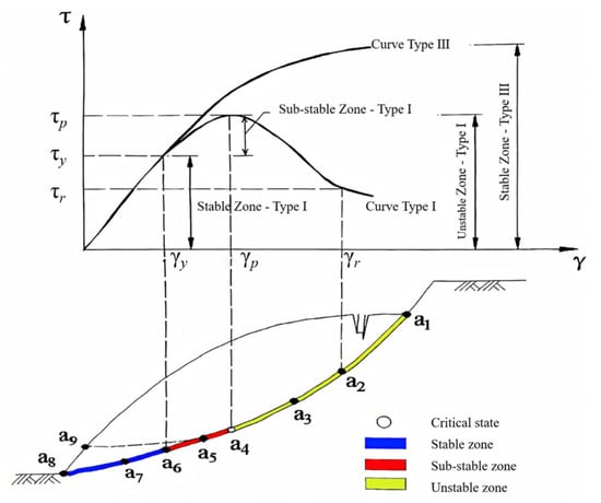
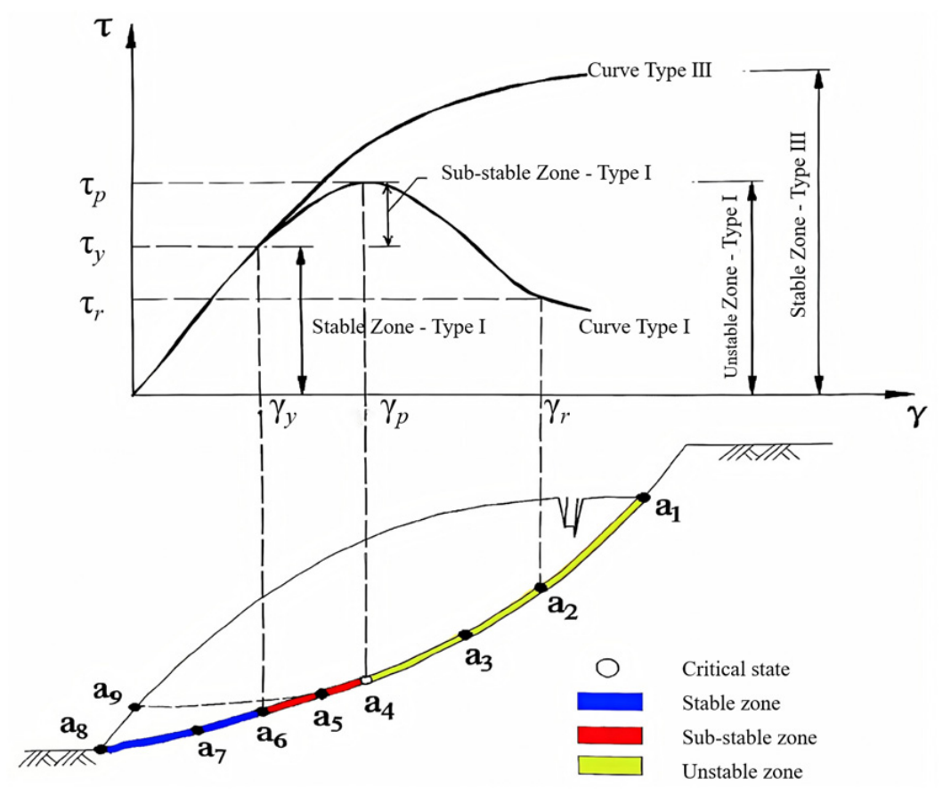
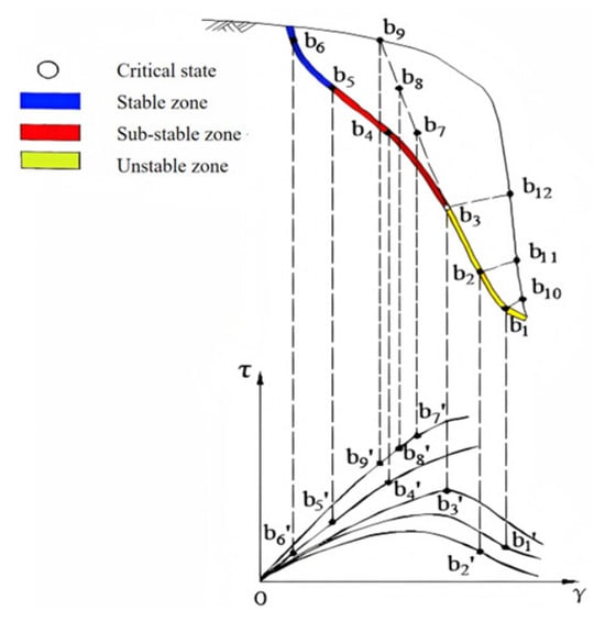
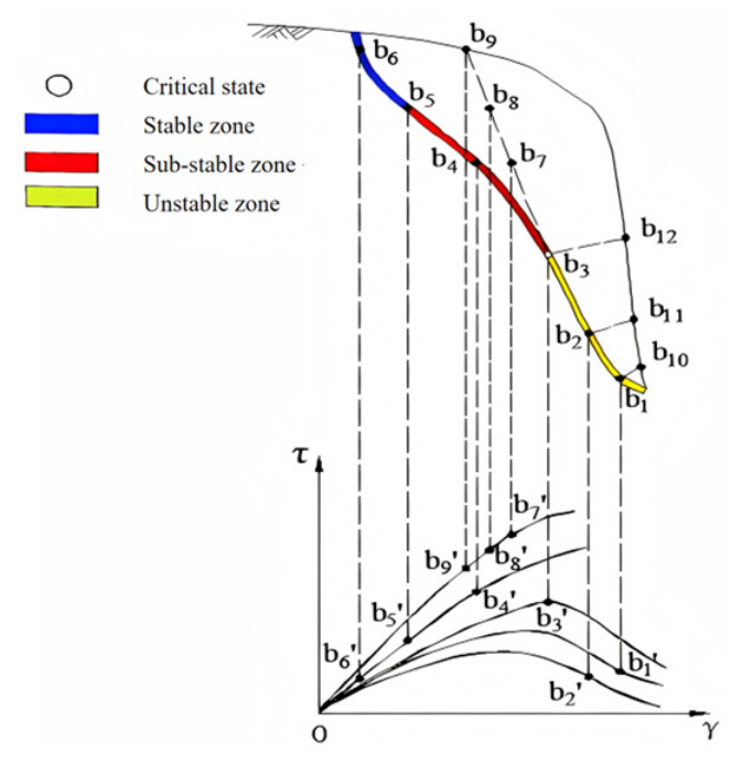
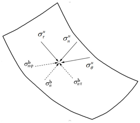
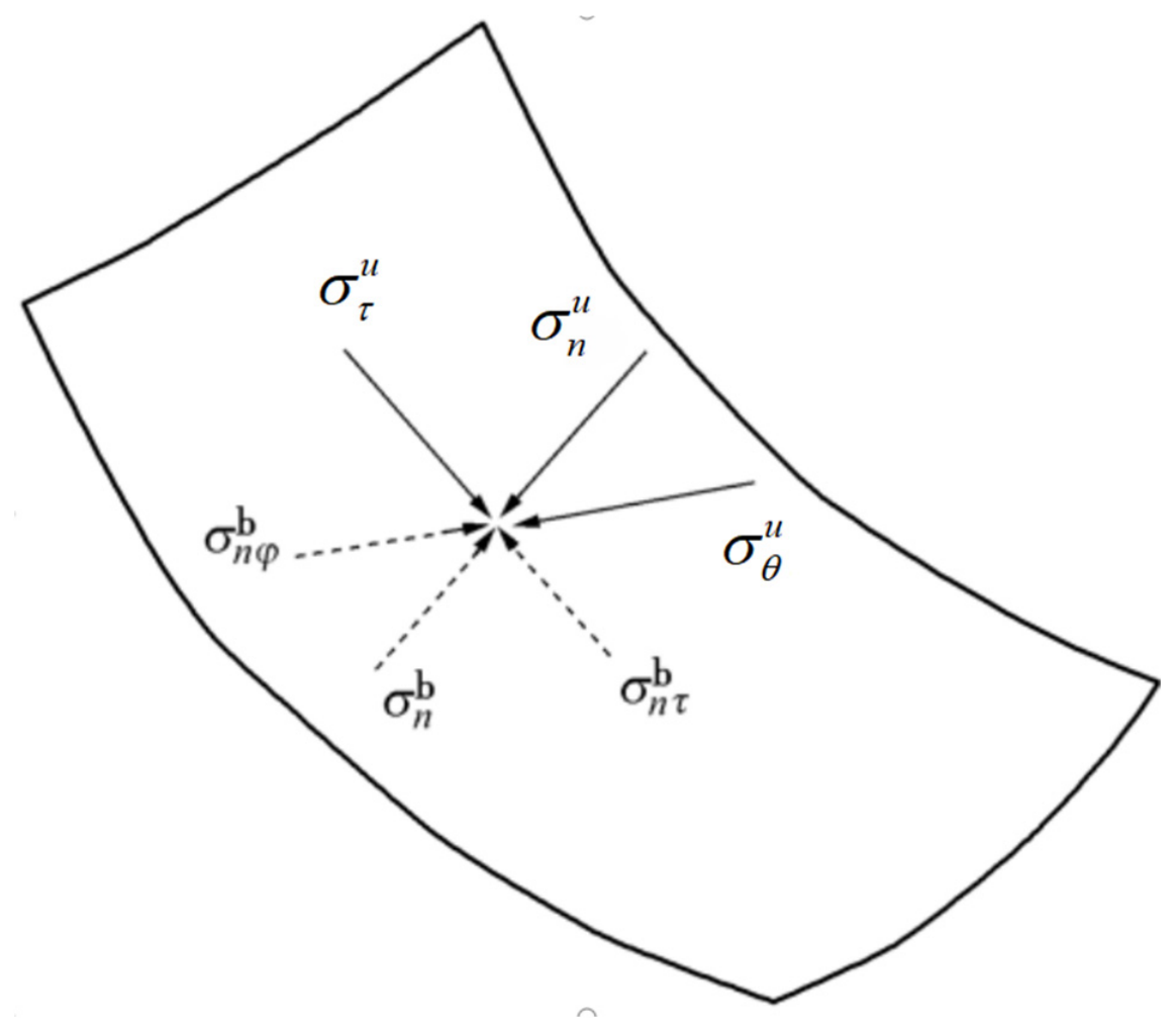
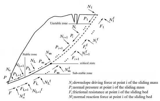
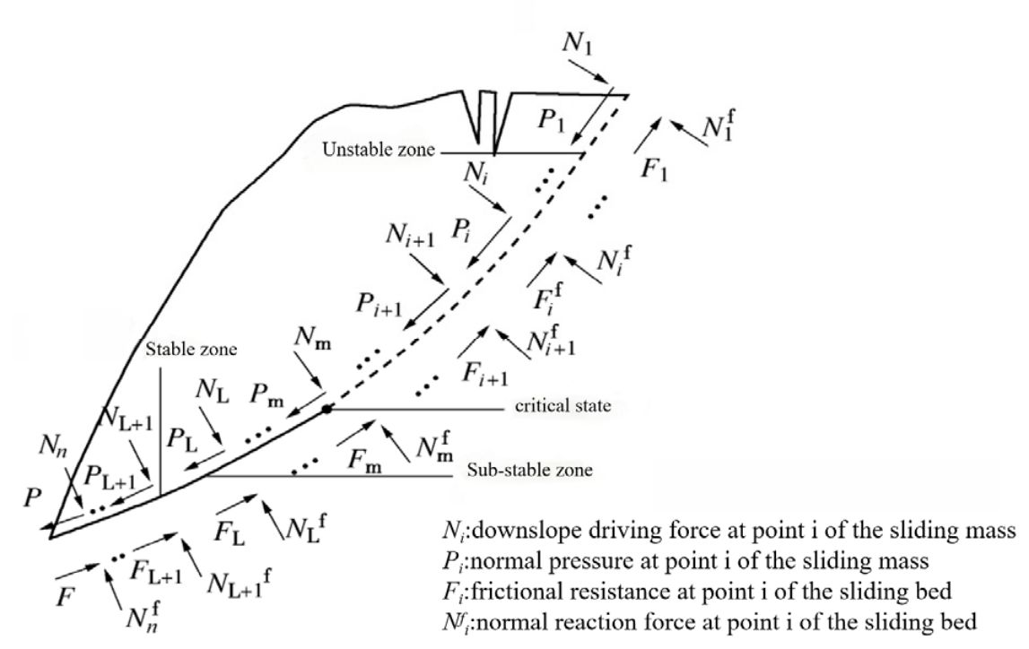
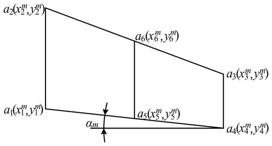
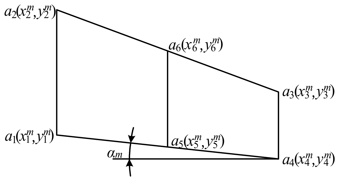
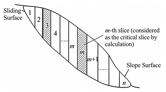
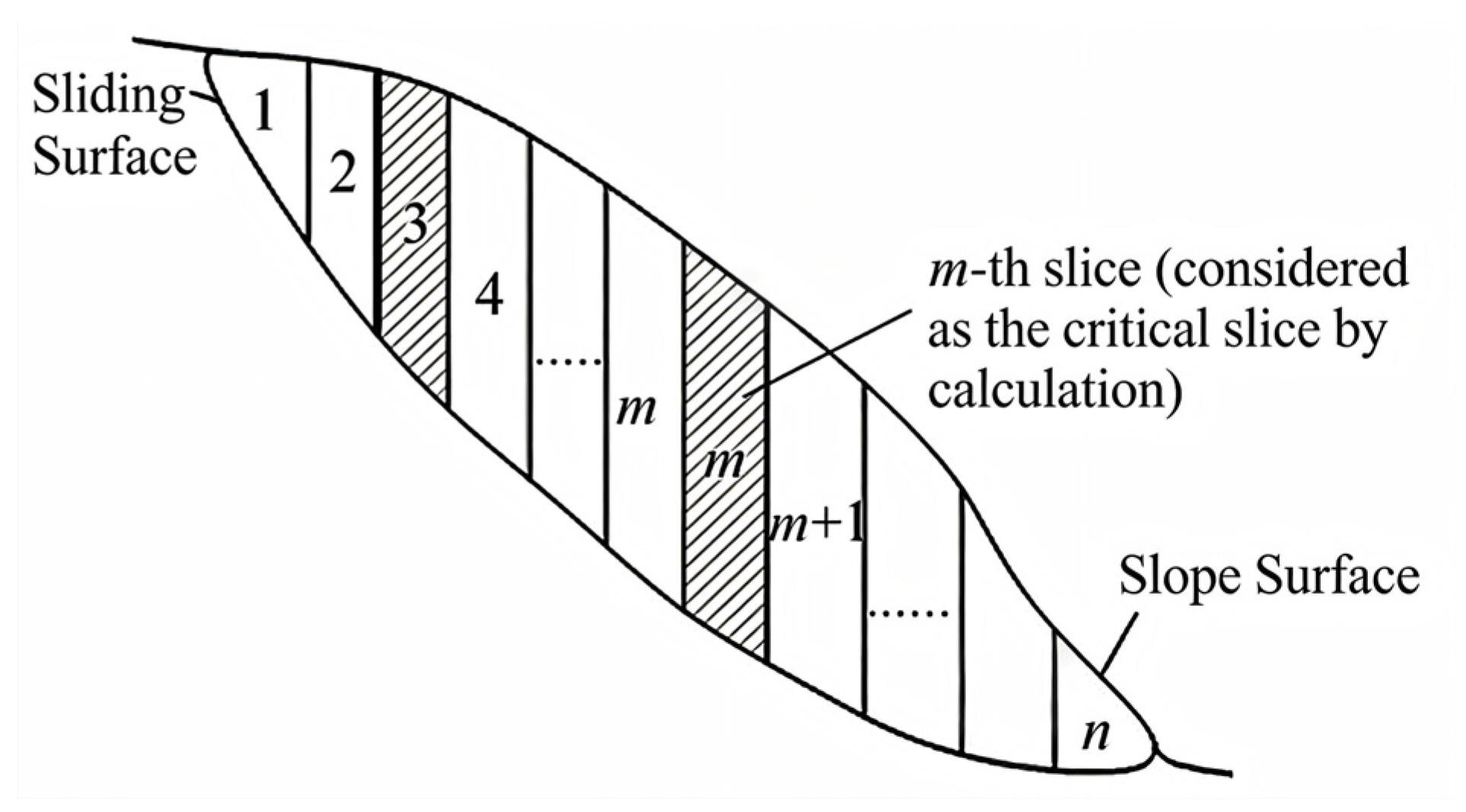
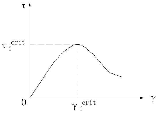
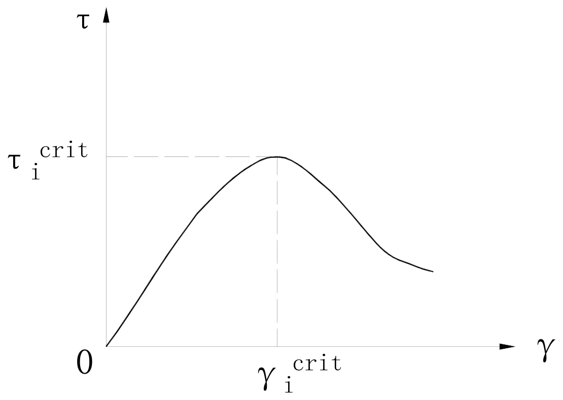
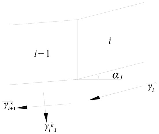
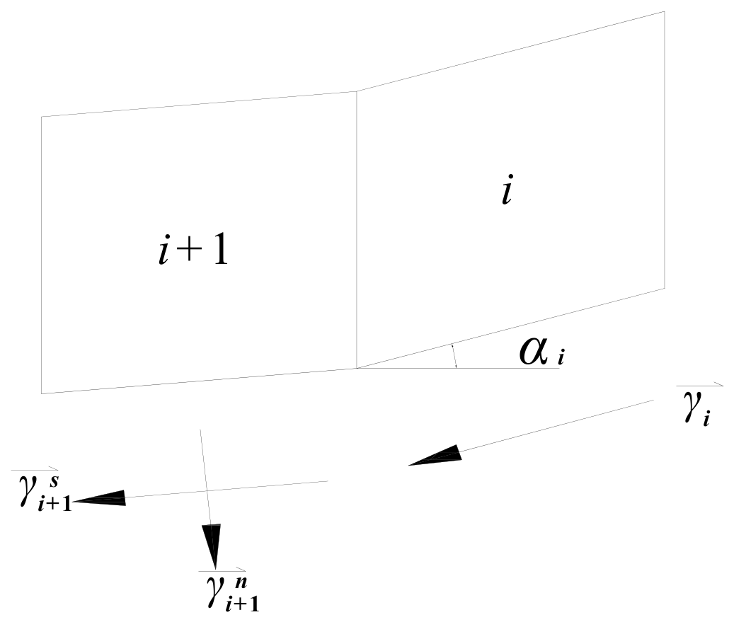
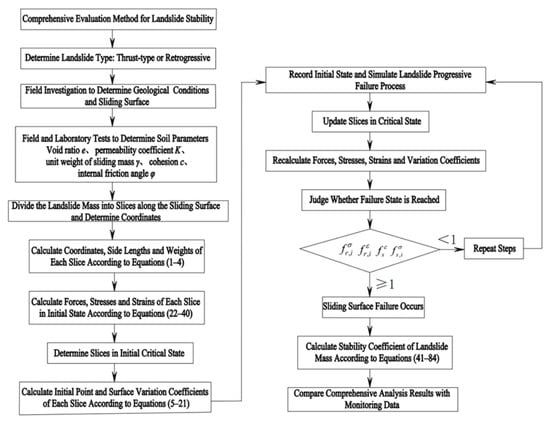
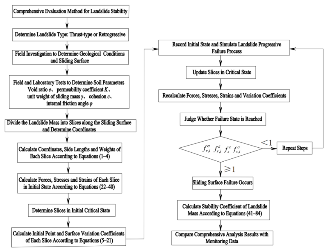
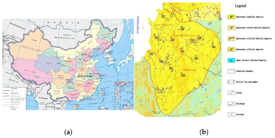
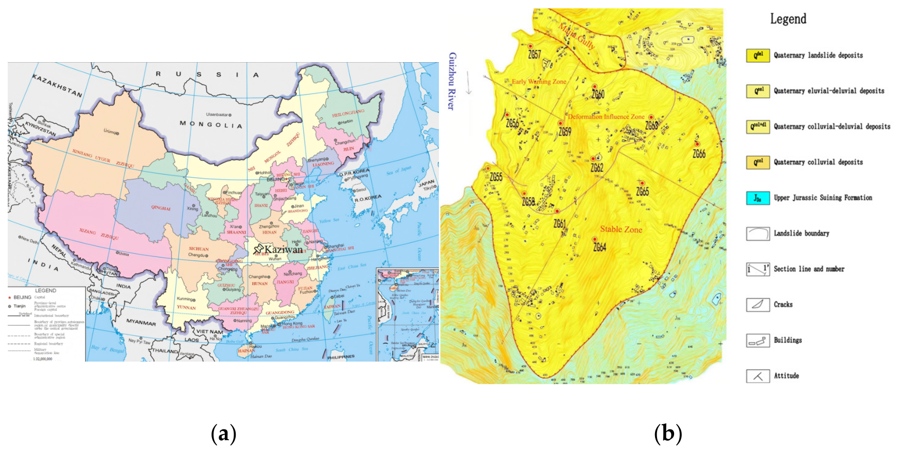
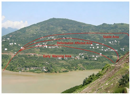
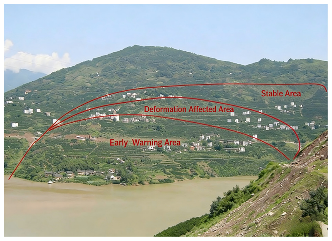
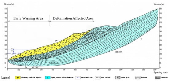
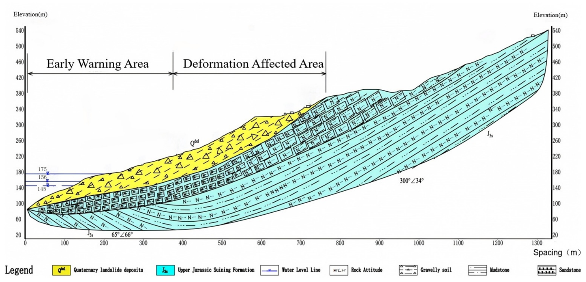
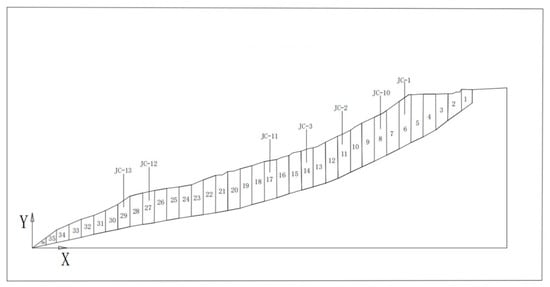
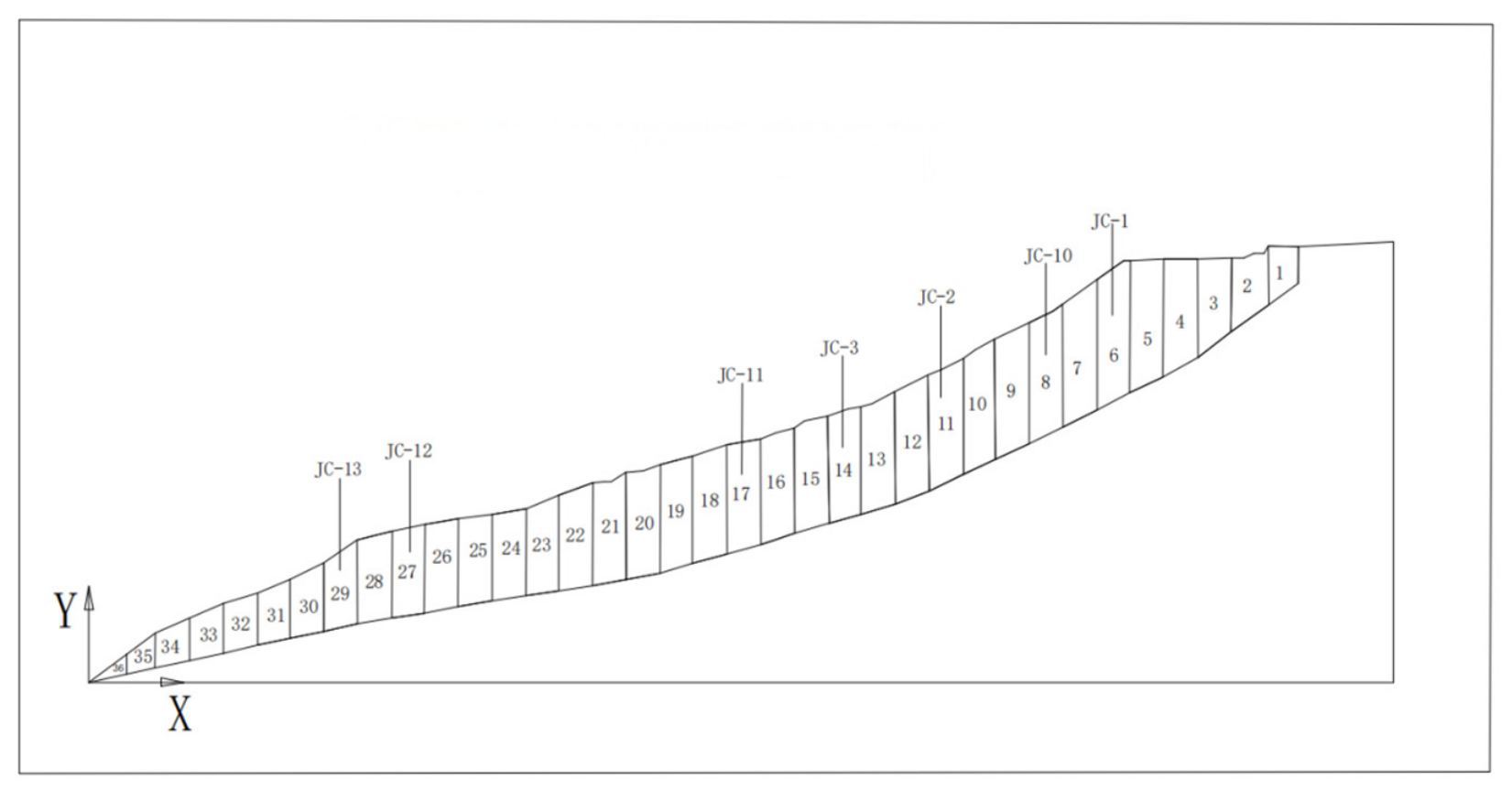
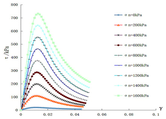
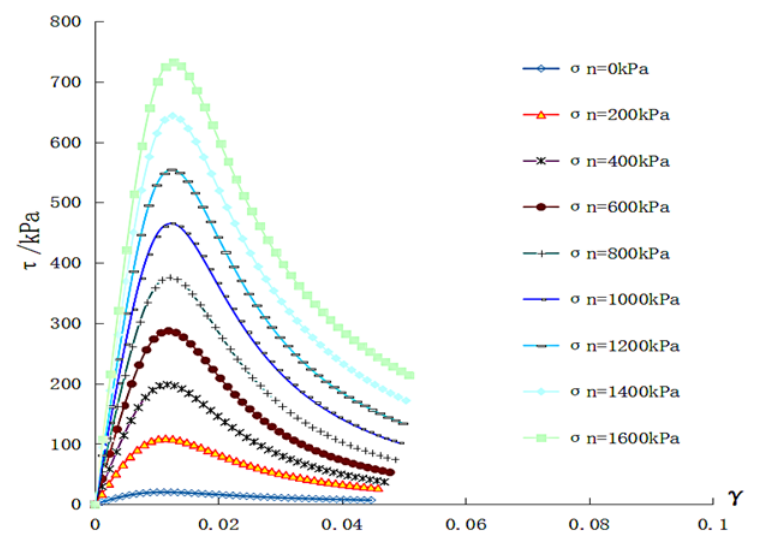
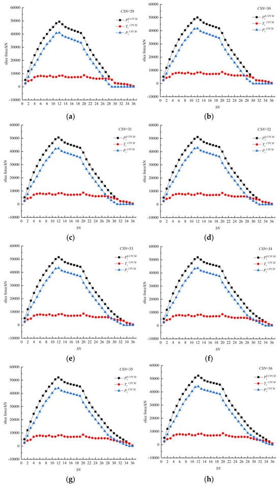
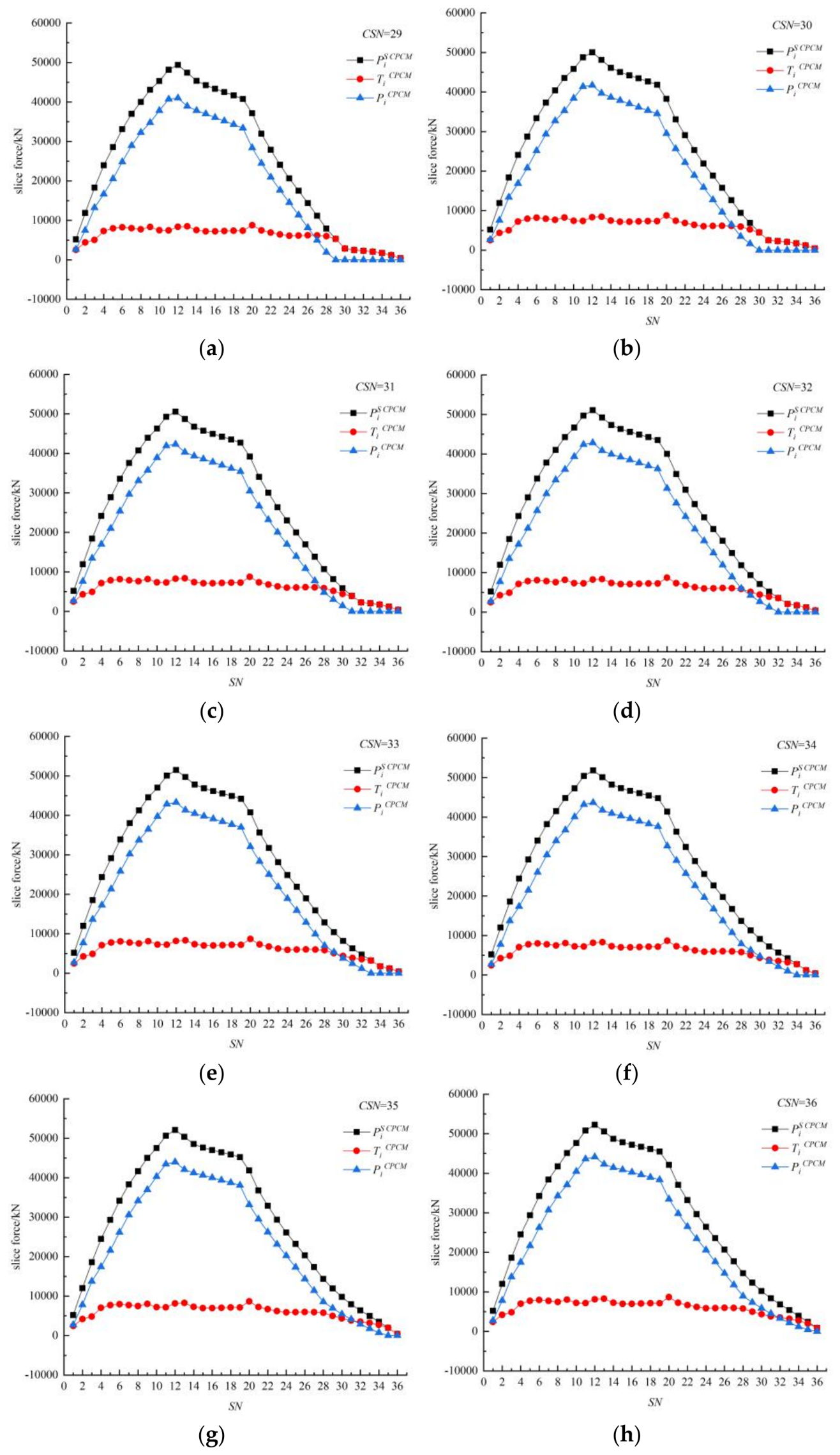
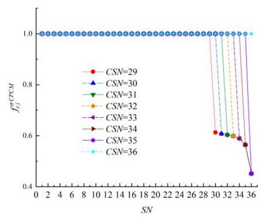
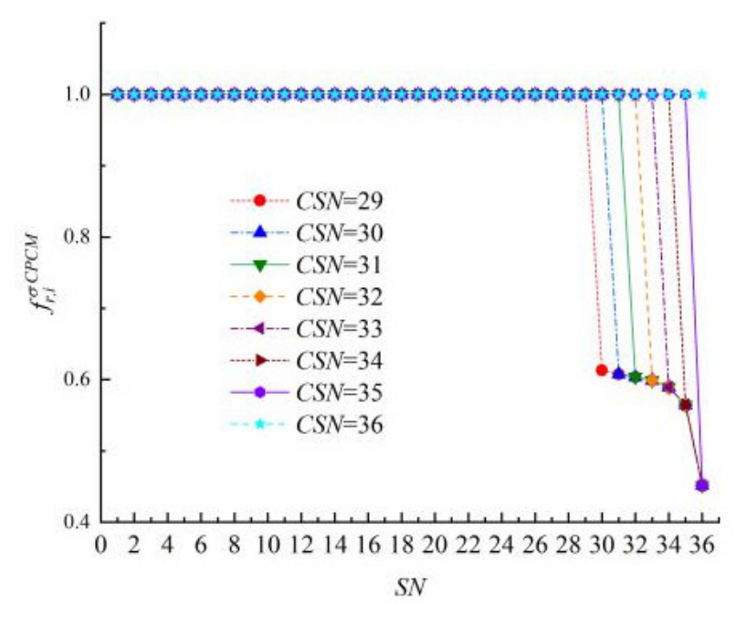
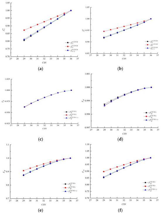
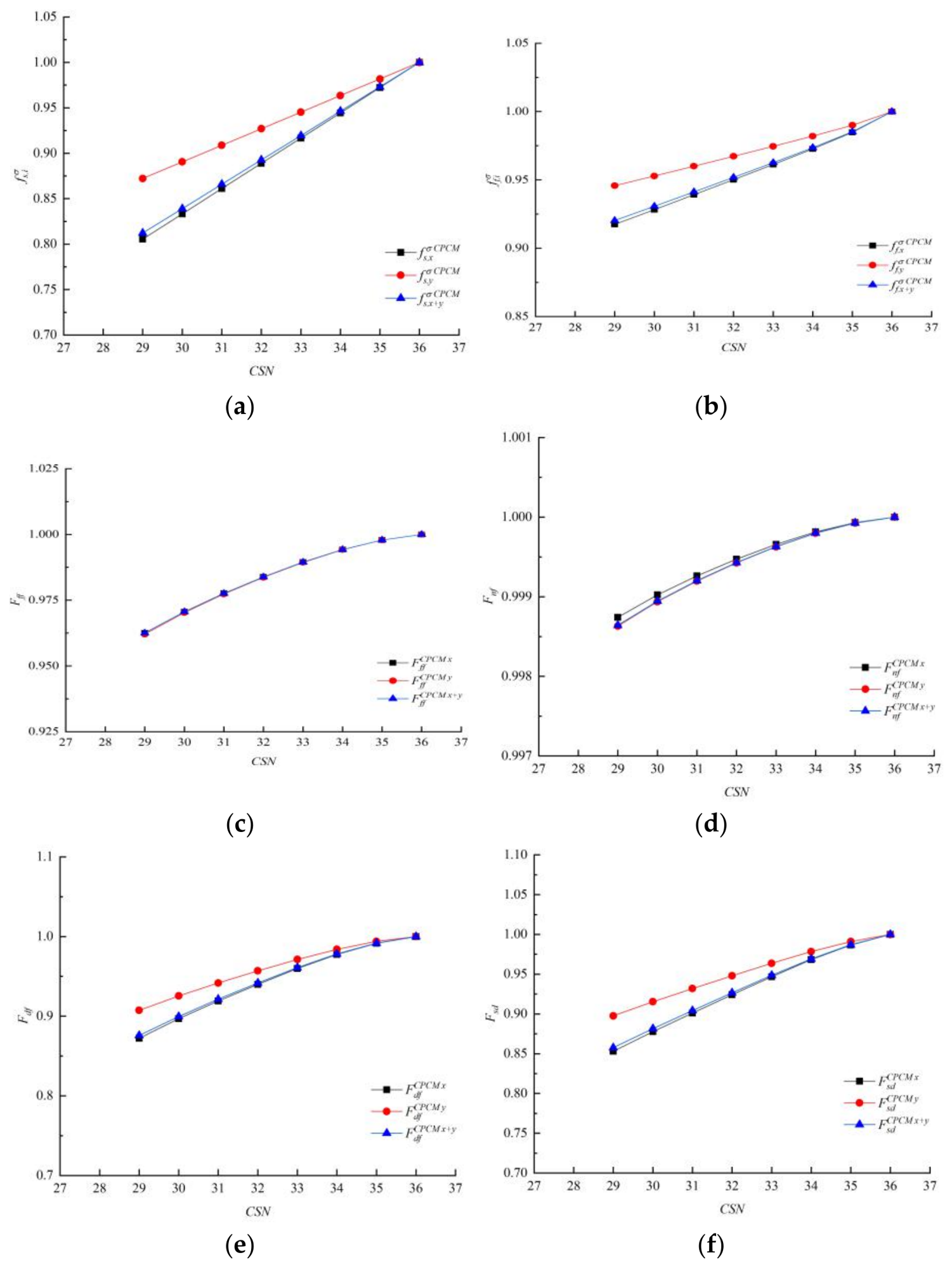
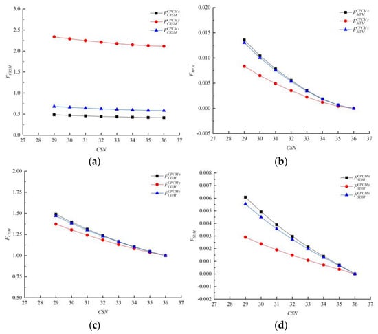
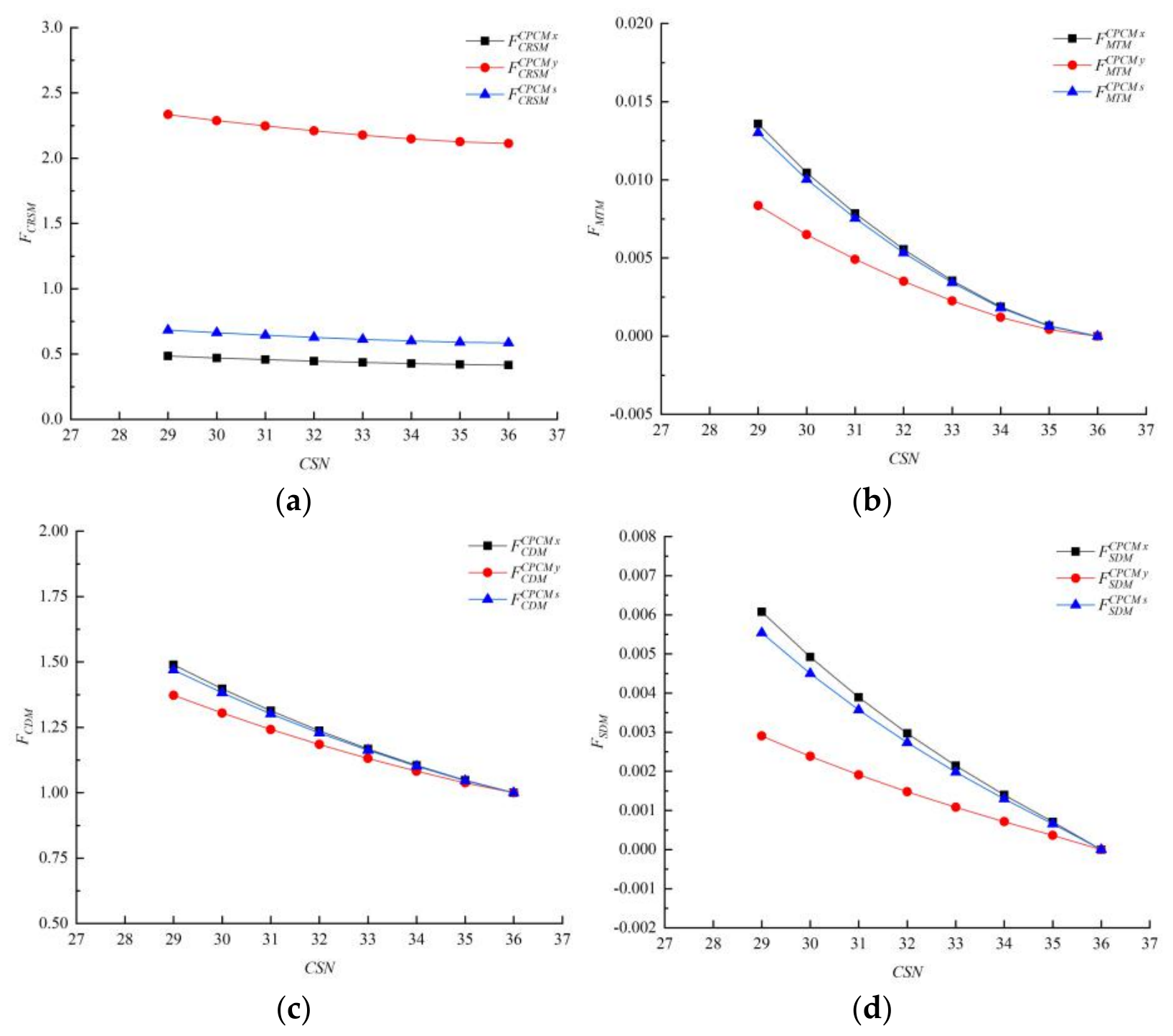
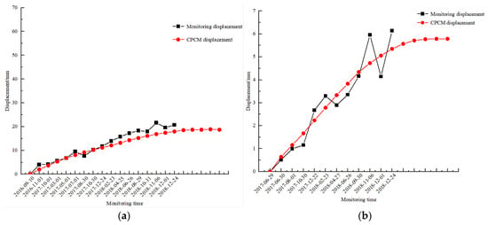
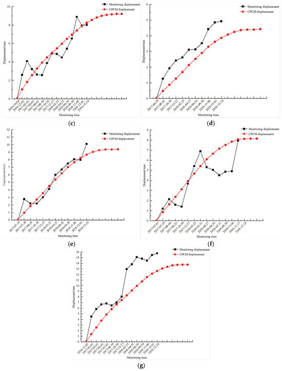
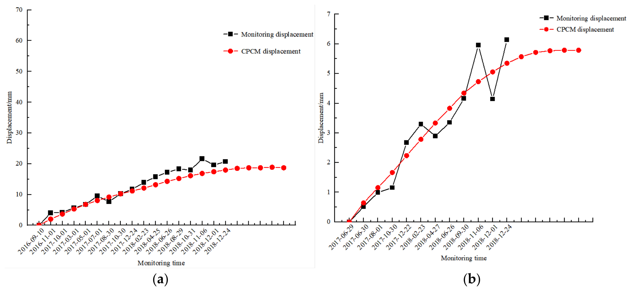
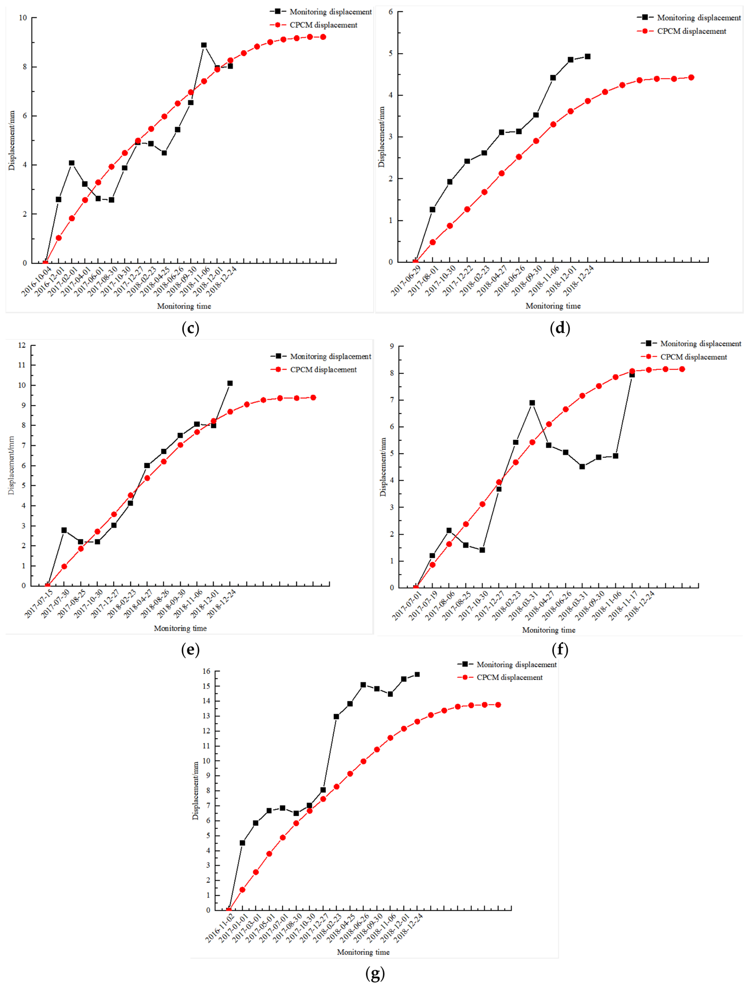

Disclaimer/Publisher’s Note: The statements, opinions and data contained in all publications are solely those of the individual author(s) and contributor(s) and not of MDPI and/or the editor(s). MDPI and/or the editor(s) disclaim responsibility for any injury to people or property resulting from any ideas, methods, instructions or products referred to in the content. |
© 2026 by the authors. Licensee MDPI, Basel, Switzerland. This article is an open access article distributed under the terms and conditions of the Creative Commons Attribution (CC BY) license.