Landscapes in the Critical Zone: Towards Geo(Morphic) Large Language Models in the Digital Earth

Abstract

Geomorphology lies at the center of the ‘Critical Zone’ (CZ) that hosts the complex interactions of weathering, soils, and the organisms in and on landscapes, reflecting geology, hydrology, slope behavior, erosion, and denudation. Many disciplines, including economics and planning, require extensive information about the CZ. This paper presents some first steps towards developing models for landscape and CZ descriptions for use within a Digital Earth framework, with the aim of promoting FAIR (findable, accessible, interoperable, and reusable) data. Fundamental to this approach is the appendage of geolocating information to digital object identifiers (DOIs) using decimal latitude–longitude ([dLL]) tuples. This enables information and data to be made digitally accessible across disciplines, as illustrated through the use of [dLL] geolocation examples of this protocol using Google Earth images. Data and image metadata are appended to a [dLL] location, creating ‘geomorphic information fields’. This schema can be easily implemented within published papers, reports, and books (Article+) using the POLE+O ontology. Appended ‘geomorphic information surfaces’ can be used to report events (such as soil loss and slope failures) that occur on these surfaces. Points with a [dLL] tuple can act as token identifiers in language/data models, as well as improve statistical analysis and the use of knowledge graphs. This paper also demonstrates ways in which data can be configured to address specific geomorphic and ecological problems and ways that digital information surfaces might contribute to the amalgamation of data from DEMs, maps, GIS, and emerging LLMs and World View Models.

1. Introduction

The progress of geoscience, as with other landscape-orientated sciences, relies on the communication of information and distilled knowledge between participants. The practitioners of the present use past information to extend knowledge bases for the future. This communication is evident in knowledge networks set up by research teams or by an individual student researcher examining library texts and online journals. Wikipedia is an open and trusted source of information and knowledge with a ‘neutral point of view’ that has been used in Large Language Models (LLMs). However, LLMs do not, despite their size, contain much detailed geoscience information, although a centralized recipient of knowledge could be Gore’s [1] ‘Digital Earth’, a ‘digital future where … all the world’s citizens … could interact with a computer-generated three-dimensional spinning virtual globe and access vast amounts of scientific and cultural information to help them understand the Earth and its human activities’ [2]. Geolocation is central to Gore’s concept. This paper promotes a simple device, decimal latitude–longitude [dLL], that can be used for digital geolocation. A [dLL] location can be used in a variety of ways that promote the identification and labeling of data and information in an ever-cluttered and often-disorganized world. Geoscience forms only a part of the information world, where ‘open’ knowledge systems are important, together with FAIR (findable, accessible, interoperable, and reusable) data. The Earth’s Critical Zone (CZ) involves geoscientists in the development of systems thinking that studies the few uppermost meters of the Earth’s crust to the top of the tree canopy [3]. This zone involves geomorphology as a study of land surfaces, which is linked to the CZ via soil science, hydrology, meteorology, and ecological sciences [4], as well as to planning and socio-political decision-making. These ever-extending knowledge bases may not be easily digitized, and thus searched, preventing information from being recognized by those with diverse interests. Scientific publishing is a knowledge field which is potentially accessible to researchers. Unfortunately, only a basic form, such as an author list, publication date, title, journal source, perhaps with keywords, and abstract, may be available after a Google Scholar search. However, problems with the ‘open’ model of publishing have recently been raised by Anderson and Moore [5] and reviewed by Montague-Hellen [6].

Geoscience knowledge bases involve images, photographs, diagrams, and data plots, as well as tabulated data and borehole logs, all with associated metadata. A problem, therefore, is how to enable this growing body of knowledge to be searched and digitized. The GeoSciML [7] provides an ‘XML-based data transfer standard for the exchange of digital geoscientific information. It accommodates the representation and description of features typically found on geological maps, as well as being extensible to other geoscience data such as drilling, sampling, and analytical data’. This is restricted to geological maps, while GeoMinLM is used for mining [8].

Searching ecological data can be aided by taxonomies, most commonly the binomial classification of Carl Linnaeus, with slightly different rules for plants and animals, then enlarged to give the six kingdoms of Carl Woese. Viruses have their own classification schemes. A different approach to organizing biological classification is cladistics, which examines shared evolutionary history rather than physical similarities or differences. Cladistics and the Linnaean classification system can be viewed as different ontologies. An ontology is a way of agreeing about language: rules noting the things—entities—that exist, how they are related, and providing an ‘explanation’ of relationships between entities. As Garcia et al. [9] noted, ‘Domain ontologies assume the role of representing, in a formal way, a consensual knowledge of a community over a domain. This task is especially difficult in a wide domain like Geology, which is composed of diversified science resting on a large variety of conceptual models that were developed over time’.

Geoscience knowledge bases encompass the persistent knowledge of entities and relationships as well as conceptual models. It is important to link these relationships to other databases, each with its own entities and ontologies of the Critical Zone, such as ecology, hydrology, and soil science, that are important in tracking and evaluating climate and environmental changes, hazards, and risks. These diverse, complex, poorly integrated and structured data and data sets and information, often with variable data quality, can be considered as part of a ‘data mesh’ or ‘data fabric’. Data fabrics are associated with accessing data, managing lifecycles and compliance and privacy, as well as data analysis and explanations. However, as Kneib and Shi [10] have noted in general, and in astronomy in particular, ‘artificial intelligence (AI) is rapidly becoming an important driver of scientific discovery’. We might reasonably ask if AI can help in earth science data evaluation, and as Large Language Models, LLM, operate on the digital literature, want to consider how these might be employed. The paper shows how some simple devices may aid data integration for searching and analysis in the context of AI and LLMs, and the ways in which ‘context engineering’—the design of systems that can assemble the ‘right’ information from institutional knowledge with tools and instructions—can fit data to the ‘context window’ of an AI system such as an LLM. The geolocation aspect of Digital Earth provides a very simple means of employing data via FAIR data strategies.

The next section contains a brief overview of words and tokens in LLMs and the idea of ‘out-of-vocabulary’ terms and the generalized structure of an academic paper, Article +. The [dLL] method for geolocation is then placed within some concepts of ‘information’. Examples of use are then illustrated and extended to suggest possible ways of operating text digitization within the realms of artificial intelligence, AI, machine learning, ML, Large Language Models, LLMs, the accompanying concept of Retrieval-Augmented Generation, RAG, and AI agents (Agentic AI). The paper also incorporates and is related to the ideas of:

• OPEN data [11,12,13,14];
• ICON Science: Integrated, Coordinated, Open, Networked [15];
• FAIR data: findable, accessible, interoperable and reusable data [14,16,17,18,19,20,21]

especially within the realms of:

• ‘Big data’ [22,23,24,25,26,27] and its stewardship [28];
• Networks and data linking [29,30].

These ideas and protocols are indicative and are not discussed in detail.

2. Methodology and Methods

This section makes some brief comments about various devices that can be used to help integrate the scientific literature, particularly applied to field sciences and the Critical Zone, into a digital world, and its utilization in AI structures such as LLMs and RAGs.

2.1. Language Structures and POLE+O

Natural language processing (NLP) is the processing of natural language information by a computer, and includes knowledge representation, information retrieval and classifications, as noted in the previous section.

Words are units of language that humans understand, but tokens are units of language that LLMs work with. Tokenization is a crucial preprocessing step in LLM training that divides text into indivisible units, tokens. Depending on the specific tokenization method, these tokens may represent characters, sub-words, symbols, or entire words.

Tokens are produced by a LLMs ‘tokenizer’, which may be different from generation to generation in any LLM, such as Claude 3 and 4. Some of the technicalities and decisions involved are discussed by Lukác et al. [31]. Responses to questions posed to LLMs depend on how questions are stated to avoid ‘hallucinations’; assertions not justified from searched information. However, there may be terms, such as abbreviations, acronyms and particularly technical terms and jargon, that may be out of vocabulary for the LLM. Typically, these are domain-specific, and some have been mentioned with respect to taxonomies. The hallucination problem has long been recognized in vision representations and, to avoid this, geological LLM versions will require the specification of typologies and ontologies, especially in the generation of Retrieval-Augmented Generation (RAG) and AI agents. A RAG is an AI framework that enables facts from ‘external sources’ to be added to an LLM’s vocabulary to reduce hallucinations.

POLE+O is a general ontology that originated in police and intelligence communities to connect disparate data, standing for Person, Organization, Location, Event plus Object. The device has been used to build general relationships and structures to tackle particular problems. The elements of a scientific paper as a citation, (author, date, title, source) or (adts), can be viewed as an information ‘chunk’ that needs to be considered as a single unit as a label in a large digital vocabulary. An (adts) chunk might be the result of a search, located by Google Scholar, within the paper itself, that the object downloaded. An author can be located by a name label or digitally using an orcid alphanumeric code as a persistent identifier. The date of the publication is usually explicit, as well as the title and keywords, included with the paper along with a reference list. The source is the journal; the issue and pages are usually given a digital object identifier, DOI. In POLE+O, the +O is an entity ‘anything else’, and we might consider it in this context as a paper’s substantive information. However, the location, L, is not generally specified digitally. It may be a mythical location such as ‘221b Baker Street’ or a mountain summit, again usually specified by a name label.

This paper uses the existing scientific literature and additions, such as images and their metadata, as a base for investigations; as Mons [28] termed it, the ‘Article(+) approach’:

‘Let’s define it as the old-fashioned scholarly communication practice upholding the tenet that the principle (sic) unit of scientific communication is the textual article with some stuff added to it (+). Figures and tables are typically still part of the paper, but supplementary data are frequently linked to it and stored in a separate location. It does not require a lot of imagination to picture how we thus create an outright nightmare for machines. Already, for example, in text-mining, the problem is imminent.’

Below, a suggestion is made that tables and figures, information entities within a paper or book, be given their own DOI, but we can combine the POLE+O idea with that of the Article(+)—whether it be an article, report, book or thesis, in paper or digital form. Linked information may be included as Supplementary Materials as Mons suggested, or in a separate repository, such as Zenodo.

2.2. Geolocation and Decimal Latitude–Longitude [dLL]

Managing information loads, data content and communication flows can be aided by simple entity digital geolocation, [dLL], as part of the Digital Earth concept [1,2]. This device and its extensions, developed below, will enable LLMs and data sets to be interrogated more flexibly. AI models will improve digital storytelling of the Earth’s surface [32] and in data management tasks. We will be able to progress beyond the use of geographical information systems, GIS, for the prediction of events on the Earth’s surface, such as landslides [33]. The use of knowledge graphs [34] towards proposals for digital twin earth [35,36] will help improve model building overall [37]. This paper explores some of these possibilities by extending the previous work on geolocation [20], within the ideas and technologies of Digital Earth [1,2] and LLM developments.

Two simple digital devices, geolocation and [dLL] [20], explained more fully below, and digital object identifiers (DOI), in addition to the traditional article reference {author, date, title, source} data set (adts), act as word-based labels linked to a DOI. The paper also develops the use of traditional nominal labels, such as ‘specimen’, ‘sample’, ‘borehole’, landscape identifiers such as ‘mountain’, and place label toponyms, such as ‘Everest’, to be digitally geolocated. This simple expedient will be meaningful for future researchers, data users, miners and analysts, as well as for general AI implementation and development [38,39,40,41] and the better use of text and images in LLM vocabularies.

3. Application of Decimal Geolocation Devices

This section provides introductions of the various ways of using decimal geolocation and using it as a ‘token’ or label to relate to other information entities such as names, place labels and authorship in the ‘information domain’.

3.1. Geolocation

If we want to know something about ‘Mt Everest’, we can interrogate the Wikipedia page; this returns 27°59′18″ N 86°55′31″ E as the summit geolocation. The conversion page gives 27.988333, 86.925278 as a six-figure decimal degree value (with an approximate ellipse of precision ~ 0.1 m). A [dLL] rounded to four figures, [27.9883,86.9252], with an ellipse of precision ~ 10 m will usually be sufficient to identify a location for most purposes. The square brackets identify the csv tuple, treated as a single value entity or primitive, that is digitally/machine searchable. A -ve latitude designates southern hemisphere and a -ve longitude as west of the prime meridian, and is elaborated in [42,43]. The general practicality of [dLL] can be seen on the AGU Landslide Blog [44] where landslide events are geolocated, usually via Google Earth, and at a specified time of observation or date of the landside event.

For Everest, the label ‘Everest’ might be replaced, or searched for, as Chomolungma, Qomolangma, Sagarmāthā, Sagar-Matha, or Peak XV; all are ‘local labels’ for the summit. A generalized label for any summit SU, a two-letter label (2LL), can be added to the [dLL]; SU[27.9883,86.9252]. For this value, a variety of associated information can be attributed as a data set and appended to the 2LL plus [dLL] labels. Such information might relate to diversity of the local names and socio-political regimes, surveying history, altitude, mountaineering history, geological and geomorphological information. This diversity can be brought together as an information set; {SU[27.9883,86.9252] {diverse information, Wikipedia entry, W*}}. Here, the local label, SU, is one of several that can be applied to mountain areas and associated with its geomorphology. This is shown in subsequent examples. In summary, the use of [dLL] geolocation allows:

1.  

Location identification and tagging supporting reader viewing and understanding.

2.  

Location identification repeat observations, especially by new methods.

3.  

Backwards compatibility and forward compatibility for locations, data and knowledge transfer.

4.  

New methods of observation used on recorded sites of interest for diverse subjects.

5.  

Data analysis and re-analysis by augmented reality in multi-dimensional spaces.

6.  

Comparisons and establishing of relations between locations, label and observations.

7.  

Comparison of data in data sets; for example, for meta-analysis.

8.  

Validity testing of theories and ideas within and across disciplines.

9.  

Integration with and extension of the FAIR and ICON concepts.

10.

Building physical landscapes and models from [dLL]-tagged data using Al/ML tools, as elaborated below.

A suite of geomorphic 2LL landform labels is being developed from several sources, including the use of [dLL] to map features, material paths and continuity in remote mountain areas [45,46,47,48] and in geoheritage [49,50]. The 2LL used below are declared in the figures and captions, and examples are used to elaborate these points subsequently.

3.2. Astronomy–Celestial Location and Information and Knowledge Networks

Astronomers have long since used a celestial system based on Declination, dec, and Right Ascension, RA, of observed objects. A mention in an article by Prescod-Weinstein [51] of the recently discovered distant galaxy known as MoM-z14, imaged in 2025 by the NIRcam instrument aboard the James Webb Space Telescope (JWST), prompted a Wikipedia search for the label MoM-z14. This gave basic information as well as its celestial coordinates: 10 h 00 m 22.40 s, +02°16′23.19 in the constellation Sextans. The NASA website [52] provides more information and metadata about the image and object. Prescod-Weinstein [51] also provided a nominal link to the original paper [53], which was identified via a Google Scholar search. The (adts) reference was downloaded, and a pdf copy was stored within my personal bibliographic database. Another paper mentioned by Prescod-Weinstein [51,54] provided a further list of authors and their orcid labels, and a browser toolbar search for the label MoM-z14 revealed yet more information. These searches produced a rapidly developing information network, independent of formal astronomical–cosmological communities. Notably, astronomical data are held in object catalogs, such as variable stars, double stars, and asteroids, and compiled in various ways, but using celestial coordinates. Geoscience has very few landform catalogs, with perhaps the most complete being GLIMS (Global Land Ice Measurement from Space) and the associated Randolph Glacier Inventory (RGI) [55].

3.3. A Geomorphological Example of [dLL] Geolocation

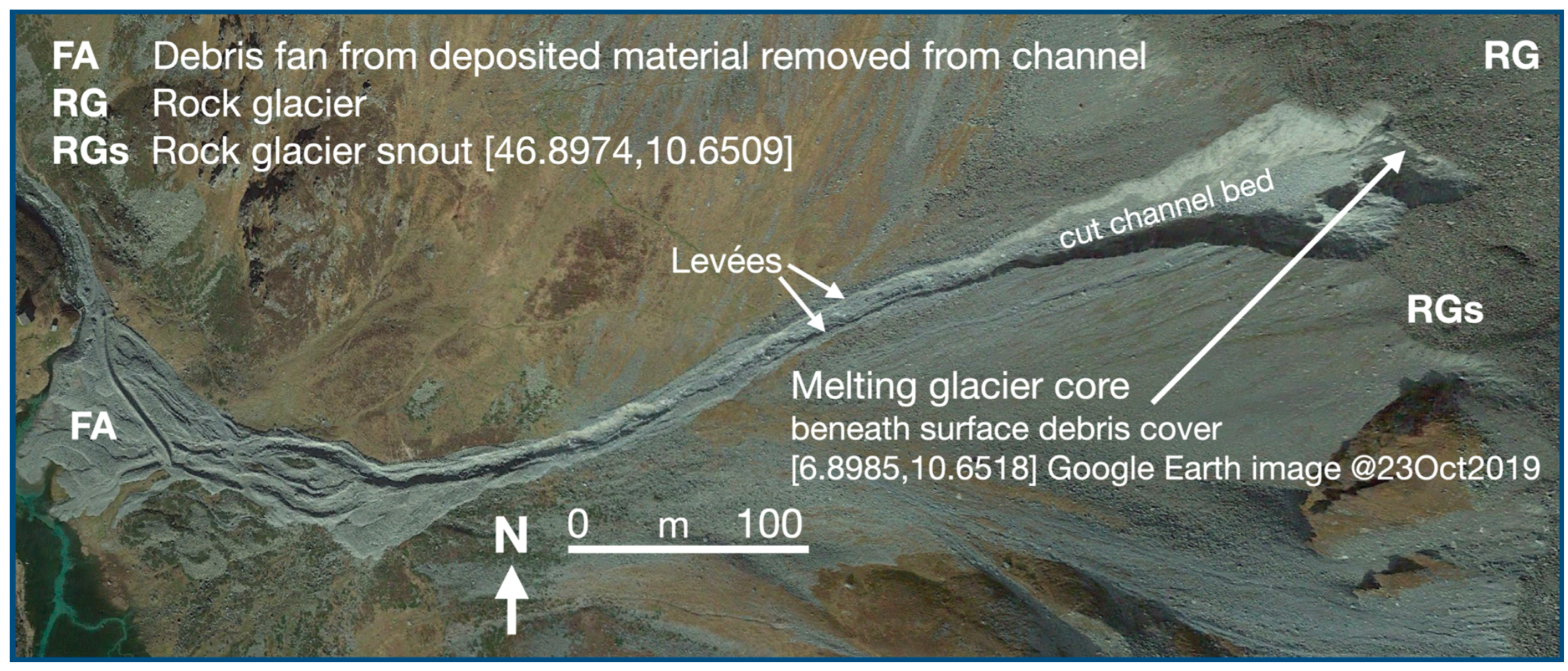
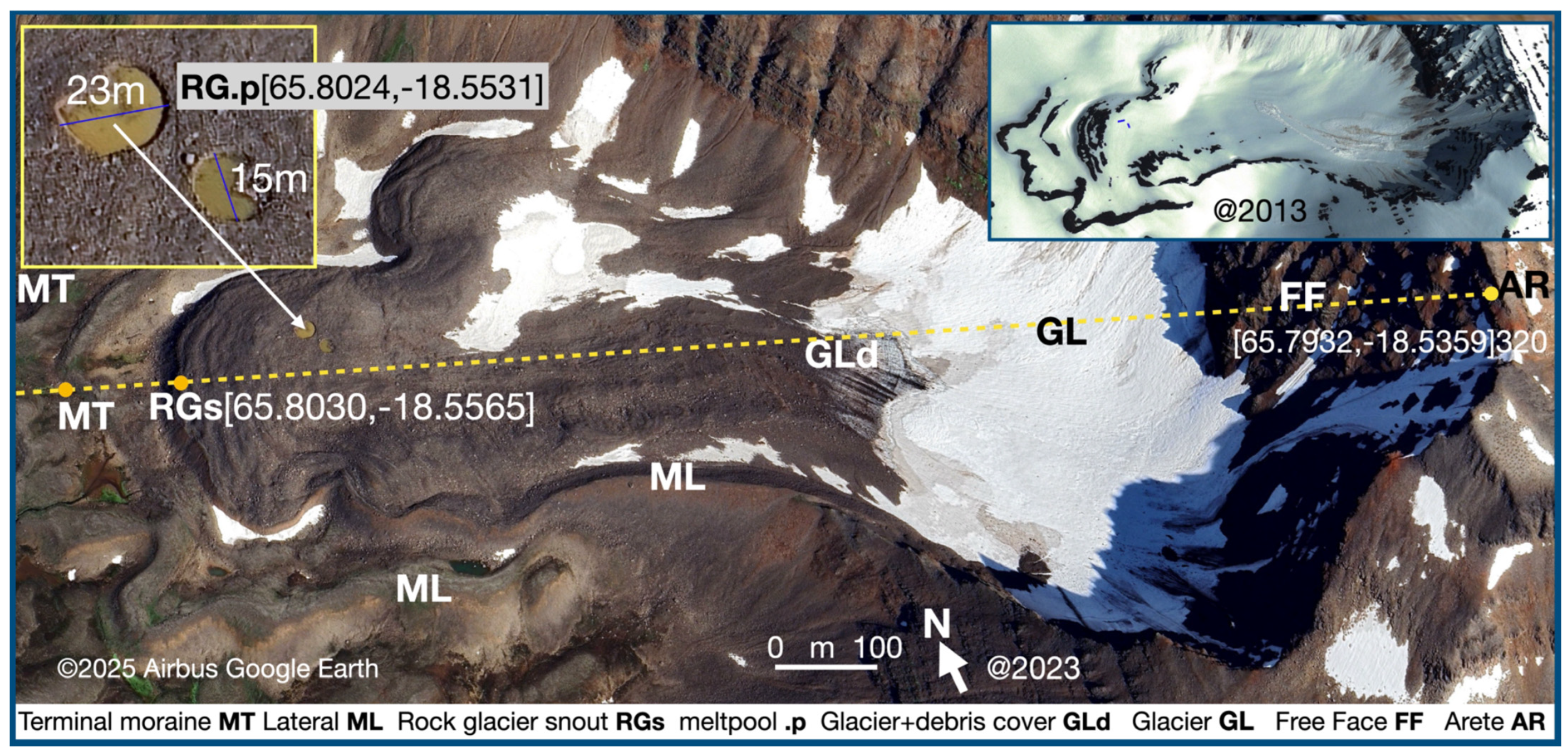
The [dLL] geolocation technique was originally developed to examine remote mountain fieldwork sites using Google Earth imagery that have become available in the last 10 years. Figure 1 gives two examples, with more data available in [42].

Papers and Article(+) referring to the rock glacier site are mentioned in the image and the caption metadata of Figure 1. Both the image and metadata might have their own DOI, although this is rare in most journals at present; an exception is PLOS One. However, although location information of the data set {Glockturmferner-Glockturm RG [46.893,10.665] {data about, [42] 10.4461/GFDQ.2021.44.4, [56]}} should turn up the image in Figure 1, the paper by Kerschner (1983), with its map, might prove elusive, even if you could track the information object in a journal in German. A Google Scholar and Cross-Ref search could not locate it, although it exists as a digitized PDF of the original paper copy in my personal bibliographic database. This raises the interesting question about the curation of information, the need for translation, and the nature of information as concept, content, digital or physical, and digital legacy of orcid scholars. ResearchGate entries may provide one postmortem data resource.

A similar situation to Figure 1 is seen in Figure 2, where an aerial and field photogaph in the literature are again compared to a recent Google Earth image with added information. The caption and metadata of the image provide much information for FAIR data requirements via the use of [dLL], 2LL annotations, and the addition of DOI.

In Figure 2, the caption shows that an annotated Google Earth image provides an open data source from which basic measurements can be taken. The .p diameters are from @2023 imagery. These could be tracked as further images are added or a field campaign planned with perhaps UAV and geophysical transects add more specific data to Figure 2 plus its caption, especially if given its own DOI.

3.4. The Nature of Information and the Digital World

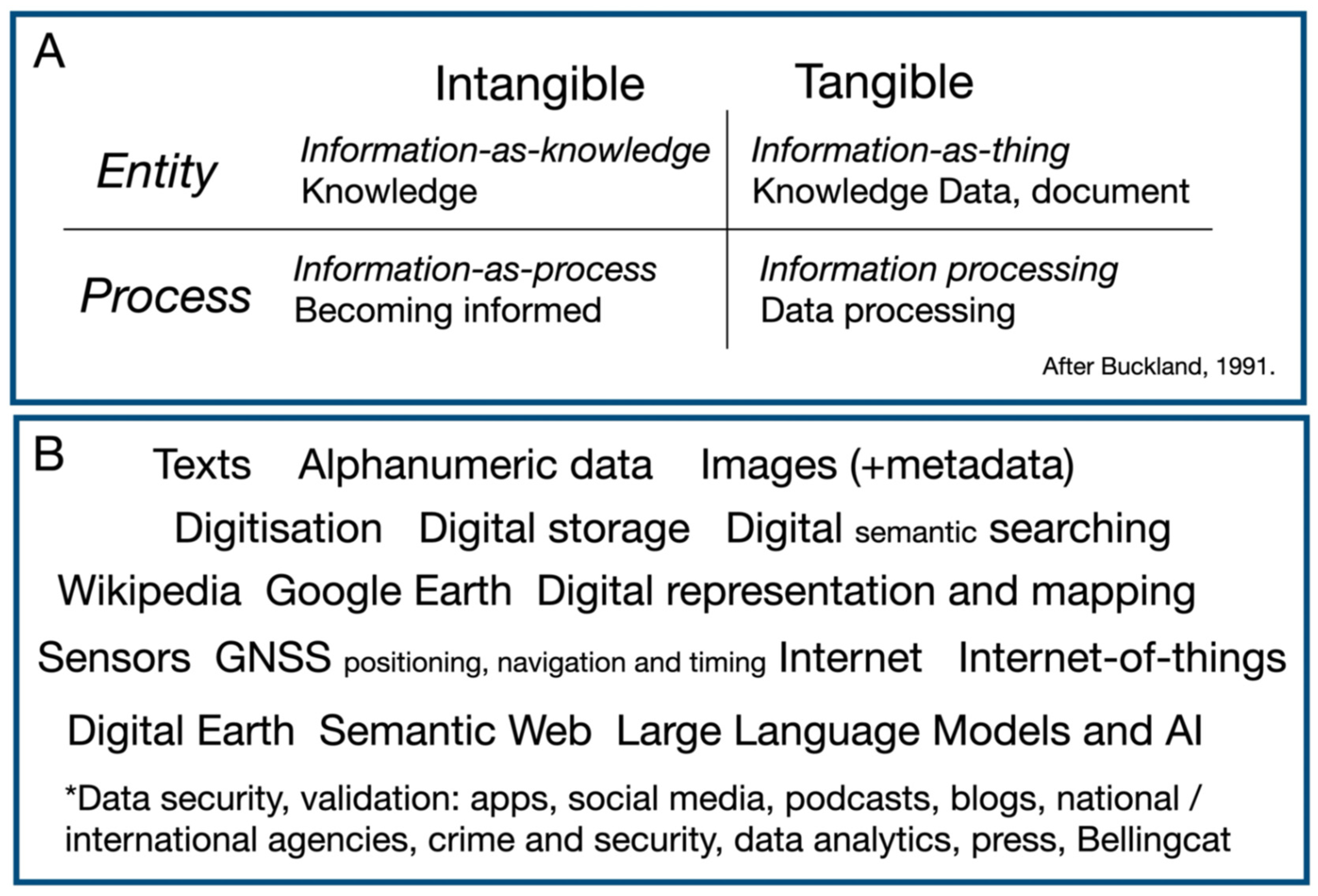
A little earlier than Gore’s ideas [1], Buckland [58] discussed ‘information as thing’ (Figure 3A). The communicated object, however, is ‘information’—information as ‘thing’, as opposed to information-as-process and information-as-knowledge [58], as in Figure 1 and Figure 2. Since Buckland, the digital world has expanded greatly, as in Figure 3B, but with the corresponding questions: Where is …? What do you mean by …? Are you certain …?. Data testing and veracity may be significant currently, as well as in LLM hallucinations.

Typically, data and information, and consequent knowledge gain, are found in papers and books that are processed and archived; a book is an example of tangible information of the Article(+) type, but such collected information may not be in a digital format and thus be digitally inaccessible.

A textbook is one form of the class, ‘book’, that can be identified and searched for on library shelves as a physical object or as meta information in a library’s searchable catalog. This catalog can be differentiated from a mere list of objects in the library, even if this is a digital library. Typically, an Article(+) entity is referenced via varying formats of author, date, title, source, or {adts}, where the curly brackets denote the set of information about the book. A book may have an ISBN, International Standard Book Number. As an example, used subsequently, the ISBN of the book ({adts}, Oliva et al., 2023 [63], Periglacial Landscapes of Europe, Springer Nature) is 3031148959 but also has a DOI: 10.1007/978-3-031-14895-8. A chapter may be specified within this as, for example, 10.1007/978-3-031-14895-8_16, which can be found in a Cross-Ref search. Although not easily digested by humans, the machine-readable format offers a way of accessing and storing information.

The kernel of an information search is the ‘current state’ of knowledge, whereas old ideas become abandoned, modified or replaced. When a new paper is published, it generally includes ‘previous work’ on the topic with some form of (adts), citation in the text and bibliography and now, a DOI can be added. But the very volume of material will only be touched up by a selected, and selective, group of references, or perhaps the first page of a Google Scholar search. This selectivity may introduce information loss: sins of omission, important material to not be cited, or even information ‘sin of commission’ to a wrong or incorrect piece of work, and, variously, such selectivity is also applicable to images [64]. Previously, the self-correcting nature of science was said to operate, but this may take some time with the pace and productivity of science. In geoscience, the acceptance of J Haren Bretz’s notion of glacial floods from Lake Missoula is an example of eventual correction [65]. There is a related problem of access for the study of old materials in geological surveys, books and theses, as well as non-English sources. Because geoscience is essentially visible, these old, non-cited or non-accessible Article(+) can include maps, diagrams, field notes and images, whether photographic, sketched, or, perhaps increasingly, videoed. The example in Figure 1 and Figure 2 and some of the issues involved in data management (Figure 3) indicate the intricacies involved.

Truth and trust are part of the scientific endeavor, but, as we become more digitally oriented into social media and the introduction of errors and ‘hallucinations’ into LLM implementation at an everyday level, thought now needs to be given to open geoscience and communication with others (Figure 3B). In other words, the data should be FAIR, otherwise the questions asked may be distorted by the digitized data available.

The operation of LLMs depends upon the splitting of words into components or tokens to produce a fundamental unit for LLM operation. Encoded tokens act as links between normal human language and the numerical values that are weighted within the LLM. For example, in an earth science context, ‘glacial’ might be one token from words split from geomorphologically common terms such as periglacial, paraglacial, epiglacial, non-glacial, pro-glacial, former-glacial, glaciated and glacierized. Different LLMs will usually have different vocabularies within which they operate and may not include all the other possible word parts that can be tokenized. The character size of a token will depend roughly on how common the word to be tokenized is in that vocabulary. Neglecting the hyphen, which might have its own token, these words are not going to be commonly found in most LLMs. For computational efficiency, the fewer tokens in a stated word the better, so a specific ‘geomorphological tokenizer’ should be better than those used by versions of ChatGPT or Claude. There is a further problem in that these words may be loosely or imperfectly defined, even in geomorphology. They may generate ‘what do you mean by…?’ questions in the geomorphological literature. Even for commonly used landform labels, we may have unclear or indistinct meanings. The case of a ‘tor’ has been used as an example [66]. But if we give any ‘tor-like feature’ (‘What I am seeing/thinking of is a tor’) the two-letter label, 2LL, TO, then its location can be specified by a [dLL]. As an example, the information set {Vixen Tor TO[50.5497,−4.0591] is a granite tor on Dartmoor that has no public access for rock climbing, W*} says a great deal about that entity and differentiates it from many other tors on Dartmoor.

Another geographical example of unnecessary tokenization is the ‘English Lake District’, often just ‘Lake District’. This is one area geographical entity with many associations (romantic poetic, William Wordsworth, tourism, geoheritage, hill farming, ecology, etc.) is best treated as {Lake District [54.428,−2.964], information about W*}. In this citation, the geolocation of three decimals suffices, and the W* is a shortform for a Wikipedia citation. The website WikiNearby, when prompted by the [dLL], but without the brackets, generates a list of other W* entries for ’nearby’ locations.

Our ‘geomorphological tokenizer’ can use, via its own vocabulary, tokens of the type [dLL] and 2LL, to which a DOI could be added. The purpose of this paper is not to invent such a piece of software but rather to show the utility of token types such as [dLL], 2LL and DOI placeholders in the literature. Other aspects of encoding, such as Huffman coding, as used in .zip, are important in building any LLM storage system, but are not considered here.

3.5. FAIR Data in the Extant Literature

Despite the commercialization of science and the publishing industry, there are moves towards ‘open science’ in data stewardship [11,12,13,28,67,68]. Taking one issue briefly, the current paradigm of scientific research—which can be taken back to the Second World War via J. D. Bernal (W*) [69,70], Eugene Garfield (W*) and the Science Citation Index [71]—is associated with the influence of Vannevar Bush [72] (W*) and his ‘memex’. Journals and books may be behind paywalls, and few university libraries will have the access to satisfy the needs of all researchers. There are also technical issues, as outlined by Mons [28]:

In open science, open access to articles is obviously desirable. However, it is a major misconception to assume that open access articles will automatically support and empower the process of open science. Data-driven science in particular can still be enormously hampered by the current Article(+) approach in scholarly communication.

The problems with the traditional print on paper text, whether textbook/encyclopedia or PDF journal, is its searchability. Although ‘AI aided’ searches, as well as the traditional Google Scholar approach, are frequently used, they tend to be semantic searches of complete Article(+) in ‘the literature’. Searches are by way of (adts) plus abstract, keywords and, in some cases, a list of supplied references. The nature of the collected data in the current and recent volumes of the ‘World Geomorphological Landscapes’ series are collections of Article(+) papers about, for example, selections of Scotland’s scenery [73]. Although they may have indexes that are useful for internal, book-specific searching, the Periglacial Landforms of Europe [63] has no index. Such books have been called ‘messy bundles’ [66] because a reference to a geomorphological site has no geolocation, and illustrations are not geolocated to where the data came from. The geomorphological landscapes are sparsely described and digital searching is inhibited. No matter how good the review and compendious the collection, the lack of georeferencing, let alone digital referencing of citations, does not allow the volume to be FAIR compliant.

There are associated difficulties in the vague use of many geomorphological terms, especially for knowledge of processes either being somewhat imprecise, ‘chemical weathering’ or vague, such as ‘nivation’, or the even vaguer ‘periglacial weathering’. To some extent, this vagueness can be moderated by more specifically looking at the geolocation and digital, DOI citation: do the answers relate to the data provided? Hence, we may return to a potential hallucination problem, ‘what do you mean by …?’. These general problems of ‘information validity’ (Figure 3B) apply particularly when many sciences are looking at landscapes, as with the Critical Zone, perhaps using different names for the same feature or phenomenon. The biosciences have an advantage over geosciences here in their use of binomial classifications and relatively rigid taxonomies. Ecological scientists may have field identification problems, as do geomorphologists.

3.6. Geomorphological Entities and the Critical Zone

The notion of the ‘Earth’s Critical Zone’ was mentioned previously. More specifically, it is the ‘heterogeneous, near-surface environment in which complex interactions involving rock, soil, water, air, and living organisms regulate the natural habitat and determine the availability of life-sustaining resources’ [74]. Gail Ashley [75] noted that,

‘The Critical Zone was originally visualized in 1998 as a way to integrate the research of the four scientific spheres (lithosphere, hydrosphere, biosphere, and atmosphere) at the surface of Earth and to study the linkages, feedbacks, and records of processes. In 2001, the National Research Council recommended that a high-priority research opportunity be established. As a concept, it was intended to be both very specific as to its context (i.e., the surface of Earth), but very broad in scope as to its potential applications. Exploration of the Deep Time variability of Critical Zones was explicitly anticipated. The Critical Zone concept represents the spirit of system science.’

Rather than closeting studies by a variety of disciplines into their respective pigeonholes, the CZ perspective provides a symbiotic framework from which the tendrils of improved understanding can radiate outward to new disciplines and/or feedback into the component disciplines. The previous discussion about geolocation and FAIR data and searches unfortunately still apply.

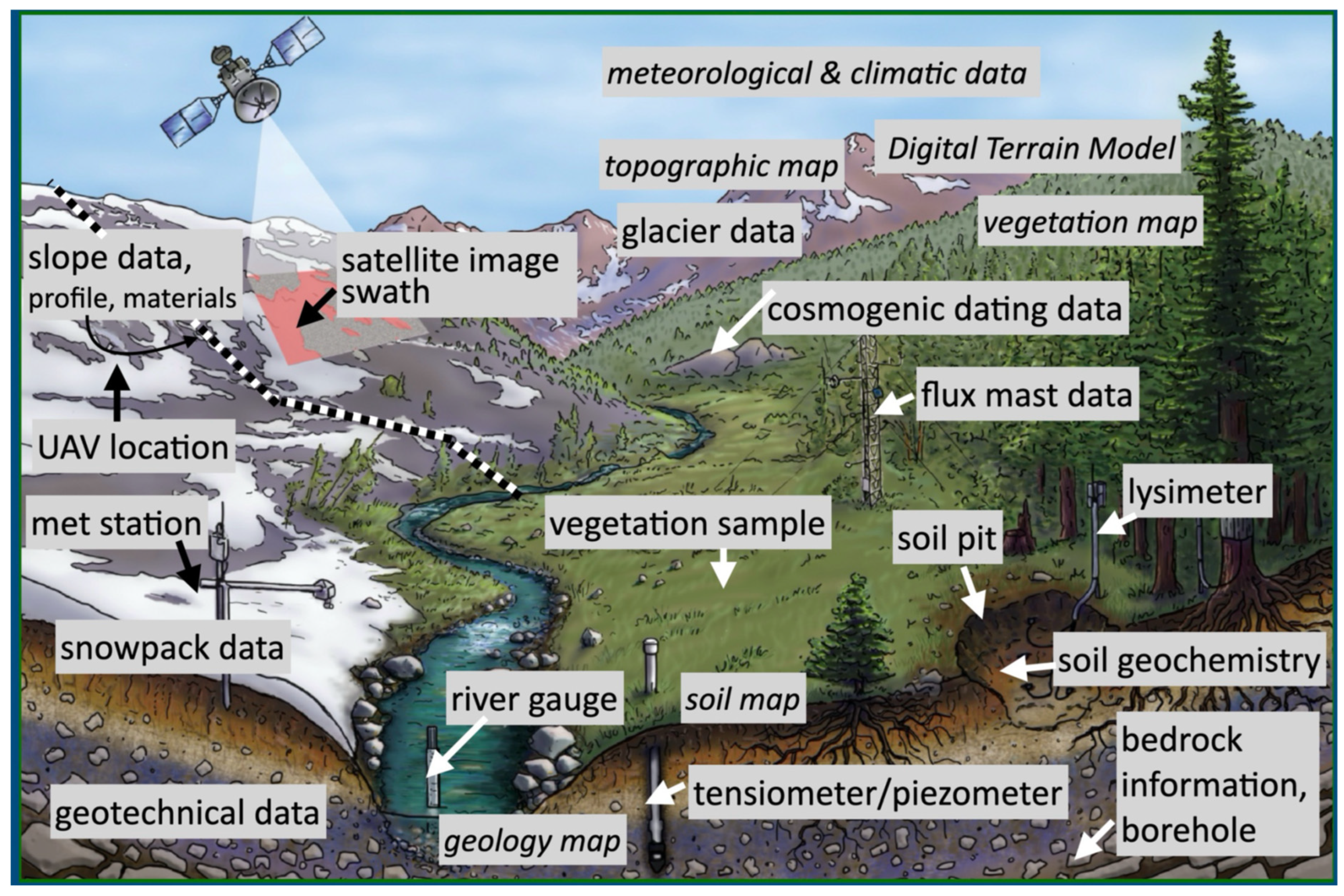
Geomorphological examination of landscapes, as in Figure 4, provides the skin on which many other studies can be based, from botany, ecology and soils to bedrock weathering, leading to hydrology and runoff chemistry. Planning and risk assessments are also significant factors, especially in light of the climate change and environmental effects of anthropogenic activity, incorporating data from many sources, as shown in Figure 4. To this might be added the literature in applied subjects, planning, risk assessment and anthropogenic change. The social scientist/philosopher, Bruno Latour, has also viewed the Critical Zone from a political perspective [76]. Some CZ data might be for the length of a project, such as lysimeter data, and incorporated into long-standing data sources such as maps and interpreted from long runs of climate data or short-term satellite data. Within scientific communication networks, an additional requirement is the appropriate integration of units, especially when dealing with areal measurements. Coordinating data gain and sharing requires the development and sharing of typologies and ontologies across several disciplines.

As each of these areas, as well as many others, are accumulating data, information and ideas in their own realms, the question need to be asked of them and by them, especially under the OPEN and FAIR doctrines: how can these information and data sets be linked? Traditionally, this is done by each Article(+) providing its own acknowledgement to the ‘previous’ literature. However, this ‘previous’ is becoming self-selective as the data lakes grow and authors use Google Scholar’s algorithm [77,78,79]. We can enquire if there are means to better collect and amalgamate these data and information. In the era of burgeoning Large Language Models (LLMs), we might ask how these might help in searching the literature. One problem to be tackled is the integration of the various ontologies for dealing with data across several study areas. For example, there are ontologies for soils [80], geology [9,81,82], soil geochemistry [83], and ecology [84,85], as well as landscapes and landforms [86,87].

The breadth of studies of these complex interactions in scientific spheres is considerable, and results are published in ever-increasing amounts, not only concerning the CZ but in related fields that may be important, especially in times of climate and environmental change. The diagram in [83] illustrates these complex inter-relationships. As well as the science per se, there are political, economic and social issues to consider, especially with respect to policy development at the local, national and international scales. The sophistication of measurement devices in the field and laboratory, as well as remote sensing and geophysical techniques in general, also add to the volumes of results in journals, theses, reports, books and from conferences. An immediate question is, how are these data to be gathered, assimilated and used effectively? Literature searches will need to operate on Article(+) with language models, but guided via agents.

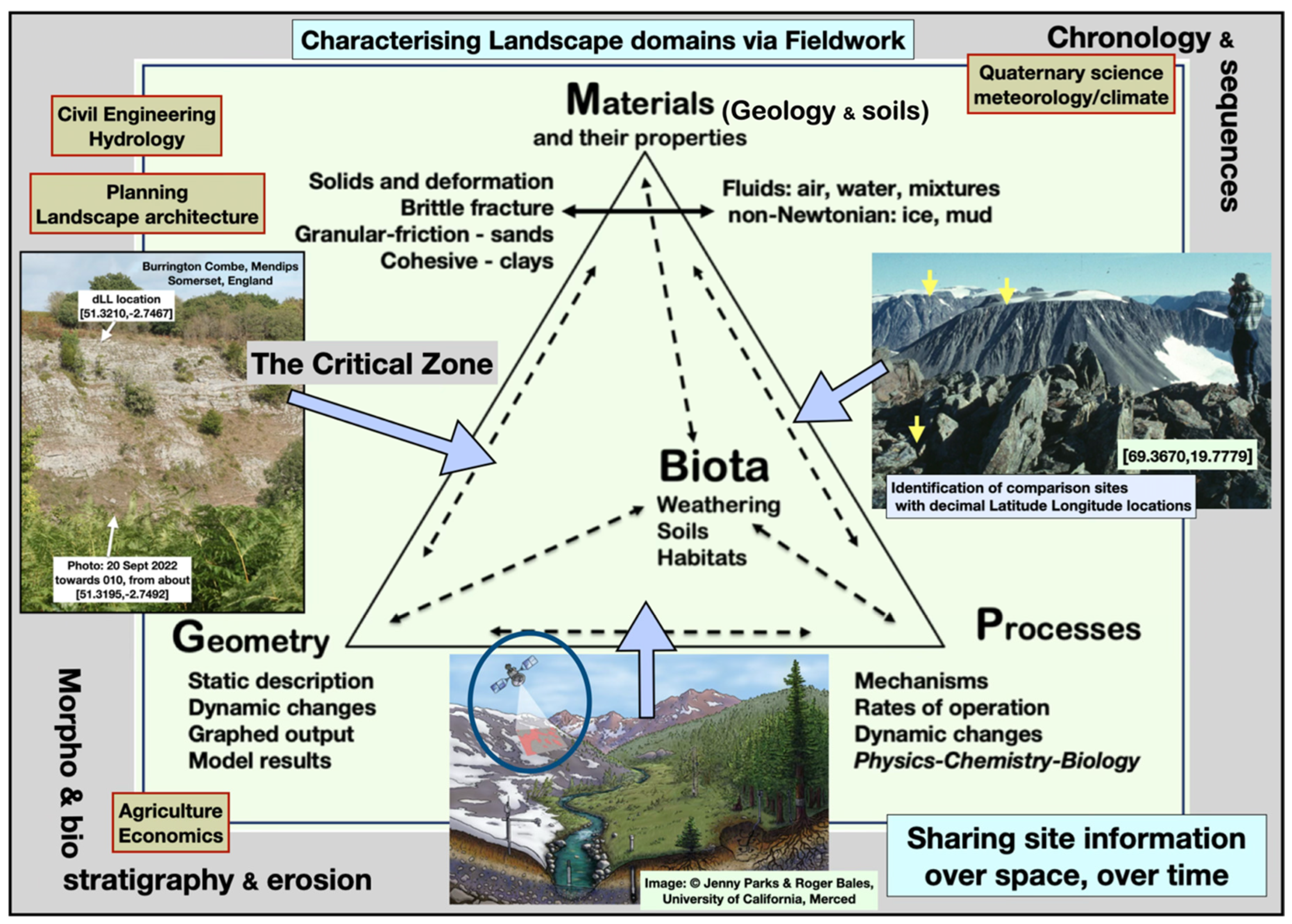
Figure 5 shows the CZ sampling point illustration with the context of the landform descriptors: Materials, Processes, Geometry and Biota—elaborated on below.

It is not shown here, but, implicit in the interrogation of landscapes by diverse sciences, is the problem of units, not least to the modelers of soil geochemistry. This is mentioned in [88], and to quote from their abstract:

‘To improve the outcomes of modeling efforts, considerations related to data accessibility and transparency in modeling practices must be addressed. Recent advancements in artificial intelligence (AI), including machine learning (ML) and deep learning (DL), have revolutionized the modeling of these interactions. This research contributes to the existing body of knowledge by identifying gaps in the literature, addressing common shortcomings in model implementation, and emphasizing the critical role of modeling in the development of sustainable water management strategies.’

The FAIR data movement is being promoted as part of ‘open data’ [14,19,89,90,91]. The complexities of coordinating searches and amalgamating data sets have only been touched upon in this paper but suggest where research targets lie in the widest geoscience remit. For FAIR data to operate effectively in mountain watersheds, for example, in Figure 4, units for chemical and solid denudation of the basin that are important for geomorphologists may differ from those used by hydrologists and soil scientists.

3.7. Decoding the Geoinformation Landscape

Earth scientists try to decode or interpret the Earth, in space and time, by using various techniques. The generalized landscape portion in Figure 3 suggests gaining information from a point that we can record as a five-decimal [dLL] as a 1 m square or circle center, of radius 1 m. This device allows us to encode elements of the landscape, which can then be built up. This 1-m-partitioned landscape has various properties but, frequently, we just use one name as a reference to such a particular landform, such as a ‘tor’. Many tors, such as Vixen Tor, have names, but others may not include the name as a label, which is why a 2LL plus a [dLL] is important in specifying a feature in a landscape or an image of a landscape. Now the area, in m², of the feature, tor for instance, is generally going to be much greater than unit square meter, although we might sample the landform at this size or smaller. As such, and like a token in an LLM, the landform is part of a vocabulary about the landscape. The larger the vocabulary, the fewer unit meter square tokens, [dLL], are required to describe the landscape. However, describing a feature, including taking an image of it, does not explain it—which is where state properties of the landform need to be investigated.

We can state that a full geomorphic description, necessary before analysis, requires describing the properties of the feature in addition to what it looks like (and is referred to in a textbook index). Calling those properties P, a description is some function of the materials, processes, as well as its geometry; P = f{M,P,G,B}, where M relates to the materials, P the processes involved and G the geometry, what it looks like, but also its size, length and area, and B relates to the biota involved. Their inter-relationships can be seen in Figure 5.

Some site data can be gleaned from a map or DEM, essentially geometric (G) slope angle and direction facing, but also from geomorphological and geotechnical maps and sections as well as field measurements. Some properties of the materials (M) are simply described, although quantitative description may still be problematic. Processes (P) are also geomorphic–geological properties and their study has become commonplace in landform studies. In summary, and in Figure 5:

Materials, M: soil type, mineralogy, weathering materials and dissolved chemicals, but may be more complex involving concepts of strength, fluid flow and rheology.

Processes, P: physico-chemical mechanisms (being integrated over time).

Geometry, G: visual form as well as size, slope angles and changes over time.

Biota, B: Natural elements which might be relevant, from bacteria to plants and a variety of animal habitats as well as interactions.

Unfortunately, geomorphic terminology can be rather imprecise and comes in three inter-related aspects: vagueness, inexactness and imprecision [92]. We have already met this with respect to glacial, periglacial, and paraglacial terms and questions about what constitutes a tor or rock glacier. This is more than an arbitrary definition and a word out of vocabulary. For example, an engineering geomorphologist will need to know the nature of the materials on a slope as these define its stability and potential hazards. A farmer and slope geomorphologist may require information with respect to soil erosion and gullying and soil losses according to seasonal rainfall on toposequences.

At a first level, these problems can be seen as a lack of knowledge of a process. Weathering is complex and complicated, and even the traditional mechanical, biological and chemical weathering are only, for the most part, terms that hide our lack of knowledge. Weathering almost always involves geochemistry, not just in carbonate rocks, but with respect to crack tip exploitation [93] and the production of clay minerals over time. As with soil development, the time period involved may be very much greater than the relatively short-term glacial history generally considered [94].

Thus, materials are intimately related to processes, and this can be seen with respect to geotechnics and engineering geomorphology. Clay slopes behave differently to granular ones such as scree. In simple terms, materials respond to applied stresses through the Mohr–Coulomb stress model. For rocks, we can consider the Hoeck–Bray model and other criteria such as Tresca but, at a crack-development, weathering scale, the Griffith criterion may be required [93,95].

The properties summarized by {M,P,G,B} can be considered as a set of state variables of a landform or a system of several landforms—a land system. State variables help define a system at a point in space or time. External, environmental variables are short-term weather/meteorological, and, together with long-term, climate ‘controls’, are classical fields. Temperature and air pressure are scalar fields and wind, from pressure differentials, is a vector. Wind speeds above a critical value can move and deposit sands in a desert. High wind speeds can abrade angular grains to give rounded grains and loess [96]. Slopes move from stable to unstable if soil stress deviators are increased by high pore water pressures from intense rainfall. These meteorological fields therefore affect the state properties at a location.

Slopes can be considered as land systems with landforms linked by the downslope movement of materials. Thus, Figure 2 shows a transect from a [dLL] starting location on a stated bearing. The transect can be shown on a map or, as it is here, a Google Earth image, with features identified over its 1700 m length covering an altitude range of ~380 m. The states of the system can be seen at @7 August 2023 and (inset) @14 June 2013. The effects of environmental fields are evident as precipitation of snow and its melt. State changes are evident as rockfalls and avalanches and the formation of meltwater pools, RG.p. The states of the system between the original observations [57] and that in Figure 2 clearly show that the constitutive expression, in continuum mechanics, for the rock glacier is that of glacier ice, the Glen–Steinemann flow law [97]. The input of glacier ice, being a continuum body, becomes overlain by insulating accumulated rock debris. The permafrost model of rock glacier flow promoted by some authors [98,99] is not applicable. The permafrost model invokes the formation of permafrost, that is, frozen soil, to be formed by mean annual temperatures < −3 °C. This is a field property integrated over time. The mechanics of the slow flow are governed by the constitutive equations. For frozen soils, even if ice-rich, the shear strength is increased by freezing—its adfreeze strength [100]. Only when scree slopes contain ice wedges thicker than ~20 m [101] will slope deformation be seen. The low-deformation creep rates, shown by rock glaciers, are easily explained by thin glaciers being protected by debris covers of around 1 m thickness. A location of [46.1761,7.9701] at Gruben RG[46.1710,7.9606] shows the rock glacier surface today, but the Swisstopo, Maps though Time, shows glacier ice with no debris cover at the turn of the 19–20 centuries [47], clearly disproving the ‘permafrost model’. These examples show the importance of relating [dLL]-specified locations with M,P,G,B properties and state conditions with changes monitored through time. Another major advantage of using this methodology is the using of the Lagrangian methodology for tracking and modeling slope conditions, including glaciers [97].

4. Discussion Using the [dLL] Geolocation

4.1. Complex Inter-Relationships in the Critical Zone

The previous section has shown the complex inter-relationships associated with even a simple section of a landscape, such as the view in Figure 4, and a geomorphologically oriented viewpoint for analysis (Figure 5). We can generally agree on calling this scene part of a topographic domain, or here, a mountain domain. Garcia et al. [9], in their investigation of a geological ontology, described some of the problems that are also relevant to the present paper:

‘In view of the data that they collect on the rocks present in the Earth surface and subsurface, geologists identify various kinds of geological objects, specify their mutual relationships and try to specify the succession of physical and chemical processes that were at work through geological times for generating and transforming rock material. Various interpretations of one geological site can be produced depending on the fields of interest of the interpreters and on the data available. Direct observation is only possible on a restricted portion of the Earth surface. It must be complemented by indirect information (seismic or well logs data), which needs to be “mapped” to the geological reality. Various scales must be considered, ranging from millimeters to thousands of kilometers. However, these technical difficulties are not the only to be considered.’

4.2. Complicated Data and Emergent Structures

Despite the landscape component complexities and possibilities for emergent structures and phenomena [102], some simplification can be achieved by considering geolocated places, [dLL], and giving features in and on the landscape identifiable labels with 2LL. The previous sections have shown how a simple and digital geolocation device [dLL] can be used to identify places, features and any identity in the field, whether using earth sciences or as locations in the Critical Zone. To this token, others, labels and DOIs can also be related to ‘tokenizing’ the landscape and can be referred to for the identifying of features for analysis or discussion. Within this arrangement, we can also consider state variables to describe the inter-relations at any point as a function of properties: {M,P,G,B}. This provides the basis for investigating and, with some forthcoming effort, combining the ontologies of the Critical Zone.

Locations identified by [dLL] can also be used to locate ‘past’ as well as current points of interest on maps, aerial photographs, and other images (Figure 2). Such ‘old’ images may be useful for the future modeling and predictions of change and response to environmental pressure within the interactions of the Critical Zone and the influence of climatic/meteorological fields.

The use of LLMs for astronomy has been indicated by, for example [103], and in molecular biology and chemistry [104]. Such advantages in using LLMs are still being discussed and developed, although a common approach for astronomy, for example in [10], still needs to be established. The present paper has mentioned some of the advantages in establishing communication groups within the geosciences, especially those studies associated with the CZ.

Digital object identifiers (DOI) have already gained a place in scientific information identification in addition to the (adts) statement for an Article(+). However, as shown in this paper, individual images and graphs, as repositories of data and information, have considerable importance; they can contain tokenized and labeled data sources. For example, the image in Figure 2 has [dLL], 2LL, data, image copyright and explanation of the 2LL used, and the caption metadata has additional, [dLL], (adts) and DOI. Text on the image can be machine readable and on the whole have its own DOI. This nesting of information using tokenized data allows for considerable progression of the FAIR concepts and data sharing.

4.3. Data Searching

Traditional data searching involves the keywords usually given in an Article(+). To this the (adts), DOI and [dLL] may be added. This may approximate searching in a ‘bag of words’ from document classifiers using natural language processing and information retrieval. Although word order is not generally important, the choice of words and what they mean can be critical, as discussed above. We also have a ‘bag of images’ and ‘bag of literature information’. Putting these bags together in meaningful ways allows semantic searching, such as with Google Search and Bing. It should be possible to collect and assimilate the large quantities of data derived from studies in the CZ. Digesting and interpreting the data will require somewhat different methods than the current bivariate regression models, even when using Bayesian methods. Without identifying a data point with its accompanying [dLL], we are likely not to use information as efficiently as we might nor make data accessible for others. When we have ‘big data’ but also expensive data, not making the data FAIR is an impediment to progress.

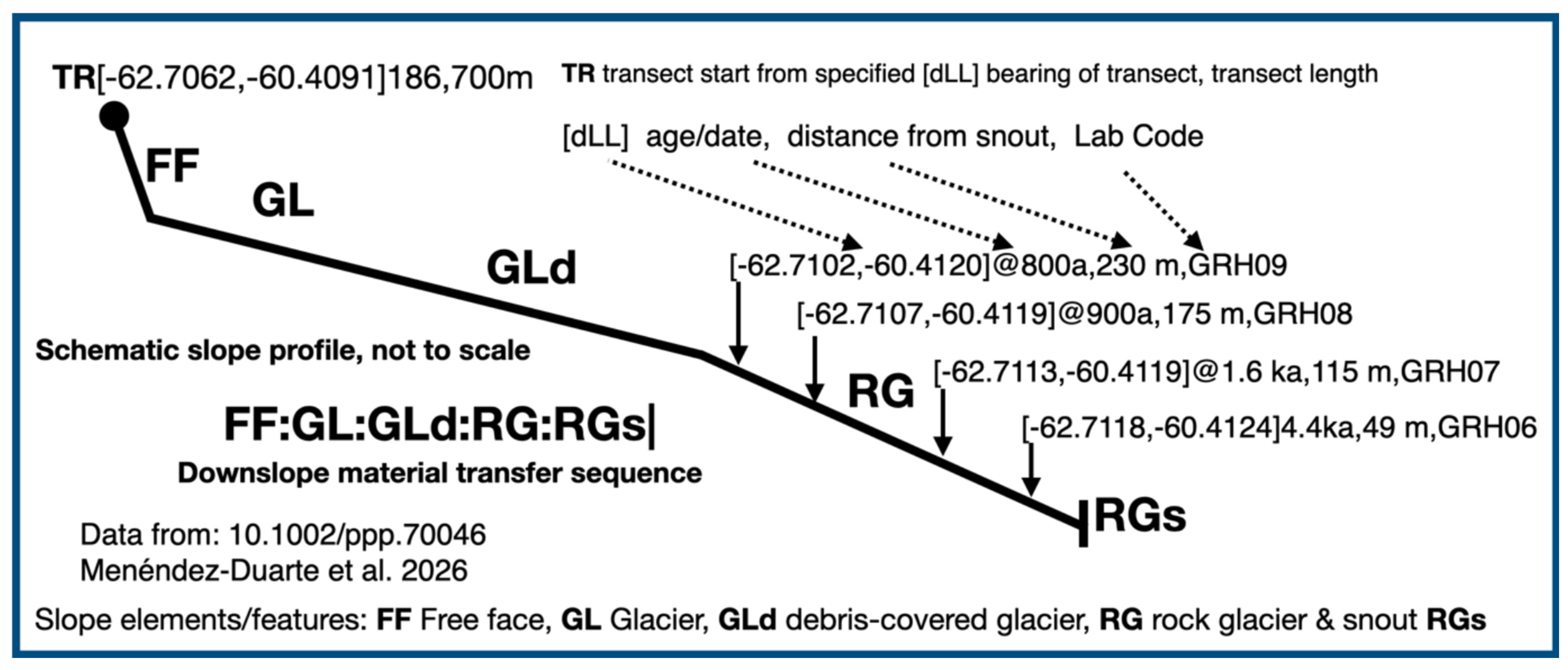
Figure 6 illustrates a simplified slope coding system mapped from Google Earth with a specified slope transect, indicated together with cosmogenic age data derived from the paper and its tabulated data. Most data tables, whether of accelerator mass spectrometry, AMS, ratios or geochemical data, have the first, or index, row value of a table as a laboratory or sample code such as GRH, standing for ‘Hurd Rock Glacier’ [105]. Here, GRH is a local label, specific to the paper, and is no use for geolocation. None of the field photographs or maps are [dLL]-geolocated and thus not FAIR compliant, and so are not helpful for the sharing of information for further investigations. The failure to geolocate sites and especially ground truth for remote sensing studies is a major problem in being FAIR compliant [21].

4.4. Agricultural Practices and the Critical Zone

The use of agricultural data is not immediately evident from the mountain domain considered in Figure 4. However, the inclusion of biota as part of geomorphological analyses of the Earth’s surface suggests that agricultural practices are very important, especially with respect to food security, international trade and climatic-weather effects. Soil loss by flooding has long been studied by geomorphologists with respect to land use [106,107] and flood routing relating to DEM data [108]. More generally, investigations [109] have looked at land use management and the need for a ‘coordinated approach to working with sensing data used to characterize and monitor agricultural land has significant potential to benefit farmers and landowners, managers, researchers, and professionals working in related domains’ [109]. Although they mention the FAIR data principles and data availability, Opitz et al. [109] also noted that substantial data sets are generated by ‘commercial and private organizations’. However, they do not consider the importance of geolocation of sites and on sites, or for communication with the Internet-of-Things [110]. For example, the use of satellite geolocation, GNSS (GPS), in precision agriculture and ‘no plough’ schemes using GNSS to reduce soils’ carbon loss are well known [111]. Detailed investigations via soil mapping and the complex processes of pedogenesis [112], including the use of soil mycorrhizal fungi, are continuing lines of research [113] that require good geolocation. Effective data sharing, especially of control trials and inter-crop comparisons, suggest that geolocation and the use of communication via Article(+) is a major area of research requiring investigation and application for policymakers.

4.5. Ways Forward with Data Structures and Representations–Knowledge Graphs

This paper has presented aspects of FAIR data and information gathering and sharing in the geosciences and CZ. However, in an age of ‘big data’ acquisition, little has been said about data analysis and data science, especially in cross-disciplinary settings. Geostatistics has long been an important part of the geosciences [114]. Although this is too big a topic to consider in detail, it is worth indicating that some methods associated with machine learning and LLMs are being employed. Tools such as knowledge graphs, in particular [115], can be helpful in investigating complex data. Knowledge graphs in the geosciences have been considered by, amongst others [116,117] and, as a commercial concern (Neo4j), has suggested that ‘The world is changing; Organizations need to transform from data to insights to knowledge’.

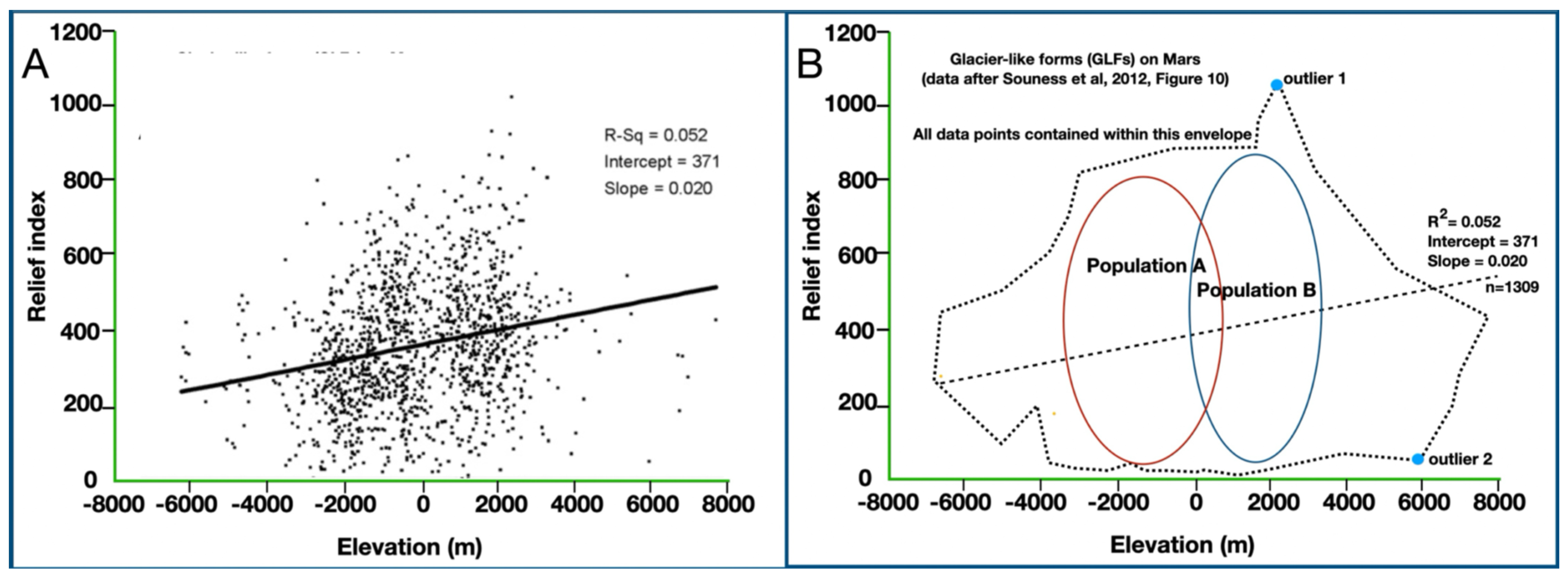
Many of the results from the ML identification of rock glaciers for the production of local inventories plot data via scattergrams, violin plots, etc. However, these graphical devices summarize descriptive data rather than explore the complex inter-site variables of materials, geometries and processes. Identification of specific features, as geolocated outliers for example, would be valuable, but, generally, such analyses are not undertaken. The data points may not in fact be independent, and confounding variables are hidden in the plotted data. Figure 7A illustrates a data set relating to surface features on Mars where nothing can be gained by simple descriptive statistics. The same point distribution is in B with an envelope containing all 1309 data points, but where ‘heat maps’, perhaps via identifying two hidden populations by canonical addition, might be useful. The geolocations of, for example, the two outliers shown, might reveal new ideas to test. Point identification by [dLL] should be an important way to visualize data sets before formal model testing.

This section has involved the notion of labels in various ways. We use the term generally rather loosely in the earth sciences, for labels of specimens collected in the field and deposited in laboratory for analysis identification. As with ‘Everest’, labels are used to denote topographic features and places: Londinium is the same ‘place’ as in Roman times, developing by the amalgamation of small villages to become the sprawling metropolitan area of London it is today. With a university such as ‘Cambridge’ (England), the question ‘where is the university?’ in one sense has no meaning other than the name given to a collection of colleges in and around the city. There are different labels here, again depending on ‘what do you mean by…?’ Nevertheless, some labels, those concerning places, do require geolocation; others may not. The following can be identified:

• General labels: landform names, soil types, landscapes, climatic types and phenomena.
• Local labels: specific, often named, features such as mountain tops, tors, glaciers that may be given a 2LL.
• Non-locational labels: laboratory identification tag on physical specimen or data result.
• Site-specific labels: linking a label, usually a local label to a [dLL] to get paired information, {label name + [dLL]}. A non-local label may need to have place information added, for example {sample of hematite, from [dLL]}.

  Table 1. Summary of main information tokens of geological features in figures of this paper. [dLL] items are header rows so that they can be used as the row identifiers. This simple device allows information to be shared, and thereby enhanced. Typically, in a paper, Article(+), the row header, is just a field or laboratory identifier specific to that paper, and does not allow for data sharing.

  [dLL]	Place Label	2LL Descriptor 1	DOIs	Figure
  [46.8974,10.6509]	Glockturmferner, Austria	RG, FA	10.4461/GFDQ.2021.44.4	1
  [65.8030,−18.5565]	Iceland	GL, RG, MT, FF	This paper	2
  [65.4933,−18.3664]	Nautárdalur, Iceland	RG	10.1080/04353676.2021.1986304	2
  [51.3210,−2.7467]	Burrington Combe, England		This paper	5
  [69.3670,19.7779]	Troms, Norway		This paper	5

  ¹ RG—rock glacier; GL—glacier; FF—free face; FA—fan; MT—terminal moraine.

  shows the main sites referred to in this paper, with the [dLL] placed first in the row. Each row can be considered an information set about that location.

4.6. Using the [dLL] Token in Information Practice

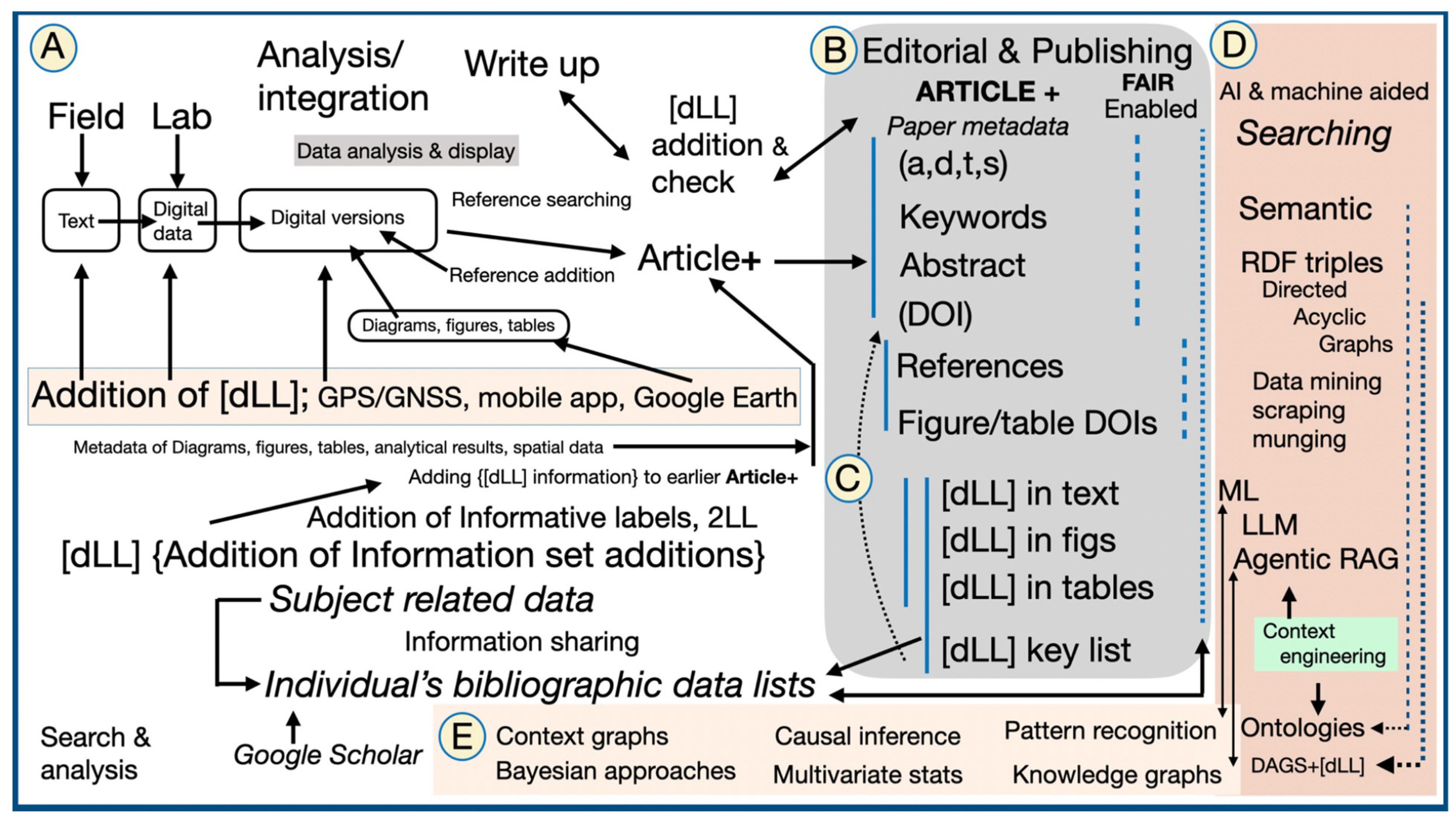
The examples used in this paper indicate how a simple geolocation primitive, [dLL], can be used to assist in the interpretation of Earth surface features, and that land systems can be analyzed by amalgamating positions with satellite-gathered information. Both can be incorporated into scientific papers, Article(+), to enhance the value of the paper. Furthermore, data sharing in Large Language Models can contribute to wider and deeper explanatory power [41]. Figure 8 summarizes, and simplifies, some of these stages.

The key to a comprehensive world model of geosciences, from landscape evolution models [119], to landscapes and landforms and their inter-relationships, {M,P,G,B}, is some way off. The Digital Earth includes the CZ, as well as related subjects of critical importance to a changing world: soils and erosion, slope stability and risk management (and its subsidiaries insurance and re-insurance), water resources, flooding, fire management and farming. These are all geomorphologically related (Figure 5) but may require data analysis in near ‘real time’. These data flows are likely to come from Earth Observation, EO, and satellite-derived and shared sources as discussed by Tuia et al. [120]. The geosciences need to encompass LLMs and incorporate the Digital Earth together with specialized LLMs in geology [8]. Geomorphological, Earth-surface-process information using ‘physics-based’ models [121] and spatially referenced information can add information into the Digital Earth for the greater good. The quirks of Earth science ontologies and classifications have been touched upon above and show that LLMs alone are insufficient. With LLMs, we already have RAGs and agents to do things, such as import data from a variety of sources and repositories. More recently, context engineering via Model Context Protocol, MCP, tools acts to accommodate these advances in AI. The nature of earth surface data requires more uniformity of access and application of the FAIR data principles.

Figure 8 highlights some of the main aspects of information addition to a basic Article(+) at stages in its preparation and beyond. The importance of locational, [dLL] information is noted in particular.

Figure 8 illustrates the complex nature of writing an Article(+). The digital attributes and addition of geolocation and other information tokens can enhance its utility in the digital information domain. The main sections are related:

• Where considered important, [dLL] from appropriate sources can be added to field and laboratory data as part of the overall data analyses. [dLL] are added to tables and diagrams, as well as a key location list.
• Journal requirements and article compilation are part of the editorial process for the article, in addition to (authors, date, title, source), keywords, abstract and DOI, which are digitally searchable and FAIR compliant.
• [dLL] are added as appropriate in text, figures, and tables and, ideally, should have their own DOI. A key location list acts as keywords and, in time, becomes searchable and digitally identified if [dLL]s are used as row identifiers or indexes.
• Machine-based searching, perhaps to produce LLM vocabularies, where [dLL], along with DOIs and orcids, act as tokens with no further subdivision. Semantic searching is aided by RDF, resource description framework, and protocols/schemas that can produce DAGs, Directed Acyclic Graphs. Data munging (wrangling) is cleaning data converting unprocessed data for use in some other form as part of data mining and scraping from websites. Context engineering places these information sources and associated data into AI structures, (LLMs and agentized RAG, Retrieval-Augmented Generation). Ontologies are part of this machine learning context engineering, an area of continued research in Knowledge Discovery in Databases (KDD).
• Areas of research and the use of ‘actionable knowledge’ in the production of AI fields such as the pattern recognition of visual and auditory information and displays, perhaps in knowledge graphs and other aspects of data science. It is in this area that there promises to be the development of ‘world models’, which, in a Critical Zone context, could include data from Earth Observation (EO) satellite data.

One aspect of geomorphology in its widest remits is the development of landscape evolution models. Despite the complexities involved with accommodating a wide variety of past and present data streams from diverse field sources, Large Language Models and machine learning offer the possibilities of accommodating them to collect, search and integrate data and information. Some of these ideas have been indicated in this present paper. One major innovation can be identified as a common means of site, landform and data geolocation; the decimal latitude–longitude tuple, [dLL]. This simple device has been shown in operation in several use cases in this paper showing current research. This paper also suggests that [dLL] geolocation should be used commonly as a major part of Article(+) and in the literature generally. In particular, the development of specialized LLMs that incorporate earth science and CZ ontologies should be promoted. For example, data fusion from its diversity and growth will be used to improve modeling [122,123].

4.7. Digital Geolocation and World View Models

The examples of use of [dLL] suggest ways to supplement traditional information components (adts) in Article(+). The examples show and link to the nature of the Earth’s surface at a point, the property set {M,P,G,B}. These state properties are easily explored and defined through fieldwork, laboratory analyses and areal compilations of data. As with [dLL] mapping, state properties and their responses to climatic fields provide rich static and dynamic models for investigating the Critical Zone. However, there are complex inter-relationships according to the intensity and duration of interacting fields, such as precipitation. Storms passing through a drainage basin that produce slope failures, soil loss and landscape degradation are typical interactions.

In its most general sense, a measurement primitive such as a [dLL], is a basic, usable protocol for coupling a physical system to an observable one to extract actionable information about system. As Willard et al. [124] stated:

‘Scientific problems often exhibit a high degree of complexity due to relationships between many physical variables varying across space and time at different scales. Standard ML models can fail to capture such relationships directly from data, especially when provided with limited observation data. This is one reason for their failure to generalize to scenarios not encountered in training data. Researchers are beginning to incorporate physical knowledge into loss functions to help ML models capture generalizable dynamic patterns consistent with established physical laws.’

Figure 8 suggests that [dLL] can be added to an Article(+) and increase the vocabulary of LLMs. But, also, in the progression from D to E, a wide variety of computational and data-display possibilities can be used to bring field data and weather–climate interactions together to allow the rapid processing of dynamic models. These may be deterministic or use physics-based models to guide best-guess, prior probabilities, and Bayesian methods for more rapid computation and data analysis. The use of causal inference methods [125] promises to be important in dealing with cross-discipline data, for example, in the digital georeferencing of epidemiological data, such as tracking ‘bird flu’, H5N1 virus cases. Examples are starting to appear in the geosciences [126]. The computational power provided by graphics processing units, GPUs, could be one way to produce World View Models using Earth science and environmental data.

4.8. Summary and Implication of [dLL] Geolocation

Geolocated dated and related devices as suggested in this paper provide a means of extending the versatility of geoscience observations, findings and data sets. Using [dLL] as a single device would assist readers of academic papers (including the general public and policymakers), as well as those sharing knowledge and data. This paper has illustrated the way journals and books, Article(+), could present enhanced information and metadata. The following is a list of suggested information protocols that would enhance information mobility, as well as making it easier for readers and reviewers to assess data and information. They apply to authors in providing the necessary FAIR data but also to assist interpretation by reviewers and readers. Journals and their editorial boards should aid information dissemination by providing tables (as in Table 1) of searchable information for AI tools on par with abstract, keyword and DOI references.

• Including appropriate geolocations of study areas, sample points, etc., with standardized [dLL] in addition to any local labels; an example is ‘Everest’. Precision to four decimal places is generally sufficient.
• Images, especially those showing sample points, ground truth sites, to be [dLL]-annotated in both the image and in metadata.
• Published data in tables to have [dLL] as row headers, thus making them digitally accessible and FAIR. Laboratory and site labels can be included as supplementary to the site [dLL]. With the sampled data points, it may be necessary to provide [dLL] to five decimal places.
• Diagrams, where feasible, to show [dLL] geolocation, such as meteorological and river gauging stations (Figure 4).
• Diagrams and tables should, if possible, have their own DOI, allowing better data searching and data integration.

5. Conclusions

The probabilistic nature of Large Language Models has allowed great advances in verbal and textual predictive power. However, LLMs operate on available text rather than the full range of data in scientific articles. The simple POLE+O ontology provides a simple structure to enable digitized tokens that encompass bibliographic data (adts), orcid personal identifiers, geolocation with [dLL] and entity labels, 2LL. The location, when given by a simple geolocation primitive of a [dLL] provides a unique and digitally convenient form to digitize locations. This paper suggests several ways in which this might be achieved via FAIR data procedures within the usual academic reporting procedures. It also suggests that further work is needed in the amalgamation of Earth Observation; other earth science data might be used in the production of World View Models. With the explosion of big data in many disciplines, especially those concerned with the Critical Zone, the introduction of simple devices to handle and search digital data and text information will become increasingly important.

References

1. Gore, A. The Digital Earth: Understanding our planet in the 21st century. Aust. Surv. 1999, 43, 89–91. [Google Scholar]
2. Guo, H.; Goodchild, M.F.; Annoni, A. (Eds.) Manual of Digital Earth; Springer: Berlin/Heidelberg, Germany, 2020. [Google Scholar]
3. Brantley, S.L.; Goldhaber, M.B.; Ragnarsdottir, K.V. Crossing disciplines and scales to understand the critical zone. Elements 2007, 3, 307–314. [Google Scholar] [CrossRef] [Scilit]
4. Giardino, J.R.; Houser, C. (Eds.) Principles and Dynamics of the Critical Zone; Elsevier: Amsterdam, The Netherlands, 2015. [Google Scholar]
5. Anderson, K.; Moore, J. How the Internet Disrupted Science; Prometheus: Essex, CT, USA, 2026. [Google Scholar]
6. Montague-Hellen, B. Change comes for science publishing paradigms. Science 2026, 393, 570. [Google Scholar] [CrossRef] [Scilit]
7. Boisvert, E. GeoSciML; IUGS Commission for the Management and Application of Geoscience Information (CGI): Ottawa, ON, Canada, 2020; Available online: https://cgi-iugs.org/project/geosciml/ (accessed on 12 July 2026).
8. Fu, Y.; Wang, M.; Wang, C.; Dong, S.; Chen, J.; Wang, J.; Yu, H.; Huang, J.; Chang, L.; Wang, B. GeoMinLM: A large language model in geology and mineral survey in Yunnan Province. Ore Geol. Rev. 2025, 182, 106638. [Google Scholar] [CrossRef] [Scilit]
9. Garcia, L.F.; Abel, M.; Perrin, M.; dos Santos, R.A. The GeoCore ontology: A core ontology for general use in Geology. Comput. Geosci. 2020, 135, 104387. [Google Scholar] [CrossRef] [Scilit]
10. Kneib, J.-P.; Shi, J. Al + Astronomy: Models, Data, Discovery. Nat. Astron. 2026, 10, 926–927. [Google Scholar] [CrossRef] [Scilit]
11. Crüwell, S.; van Doorn, J.; Etz, A.; Makel, M.C.; Moshontz, H.; Niebaum, J.C.; Orben, A.; Parsons, S.; Schulte-Mecklenbeck, M. Seven easy steps to open science. Z. Für Psychol. 2019, 227, 237–248. [Google Scholar] [CrossRef] [Scilit]
12. Dienlin, T.; Johannes, N.; Bowman, N.D.; Masur, P.K.; Engesser, S.; Kümpel, A.S.; Lukito, J.; Bier, L.M.; Zhang, R.; Johnson, B.K. An agenda for open science in communication. J. Commun. 2021, 71, 1–26. [Google Scholar] [CrossRef] [Scilit]
13. UNESCO. Understanding Open Science; UNESCO: Paris, France, 2022; Available online: https://unesdoc.unesco.org/ark:/48223/pf0000383323 (accessed on 12 July 2026).
14. Hasnain, A.; Rebholz-Schuhmann, D. Assessing FAIR data principles against the 5-star open data principles. In Proceedings of The Semantic Web: ESWC 2018 Satellite Events: ESWC 2018 Satellite Events, Heraklion, Crete, Greece, 3–7 June 2018; Springer: Berlin/Heidelberg, Germany, 2018; pp. 469–477. [Google Scholar]
15. Burberry, C.M.; Flatley, A.; Gray, A.; Guilinger, J.; Hamshaw, S.; Hill, K.; Mu, Y.; Rowland, J.C. Earth and planetary surface processes perspectives on integrated, coordinated, open, networked (ICON) science. Earth Space Sci. 2022, 9, e2022EA002414. [Google Scholar] [CrossRef] [Scilit]
16. Lehnert, K.; Wyborn, L.; Klump, J. FAIR geoscientific samples and data need international collaboration. Acta Geol. Sin.-Engl. Ed. 2019, 93, 32–33. [Google Scholar] [CrossRef] [Scilit]
17. Kinkade, D.; Shepherd, A. Geoscience data publication: Practices and perspectives on enabling the FAIR guiding principles. Geosci. Data J. 2022, 9, 177–186. [Google Scholar] [CrossRef] [Scilit]
18. Wyborn, L. One Geoscience: Providing FAIR Global Access to all Geoscience Data-Are We There Yet? NCI Australia: Acton, Australia, 2023. [Google Scholar]
19. Jacobsen, A.; de Miranda Azevedo, R.; Juty, N.; Batista, D.; Coles, S.; Cornet, R.; Courtot, M.; Crosas, M.; Dumontier, M.; Evelo, C.T. FAIR principles: Interpretations and implementation considerations. Data Intell. 2020, 2, 10–29. [Google Scholar] [CrossRef] [Scilit]
20. Whalley, W.B. Enhancing the Digital Earth via digital decimal geolocation and the FAIR data principles. Earth Sci. Syst. Soc. 2024, 4, 10110. [Google Scholar] [CrossRef] [Scilit]
21. Whalley, W.B. Remote Sensing and Landsystems in the Mountain Domain: FAIR Data Accessibility and Landform Identification in the Digital Earth. Remote Sens. 2024, 16, 3348. [Google Scholar] [CrossRef] [Scilit]
22. Hampton, S.E.; Strasser, C.A.; Tewksbury, J.J.; Gram, W.K.; Budden, A.E.; Batcheller, A.L.; Duke, C.S.; Porter, J.H. Big data and the future of ecology. Front. Ecol. Environ. 2013, 11, 156–162. [Google Scholar] [CrossRef] [Scilit]
23. Gattiglia, G. Think big about data: Archaeology and the Big Data challenge. Archäologische Informationen 2015, 38, 113–124. [Google Scholar] [CrossRef] [Scilit] [PubMed]
24. Chen, L.; Wang, L.; Miao, J.; Gao, H.; Zhang, Y.; Yao, Y.; Bai, M.; Mei, L.; He, J. Review of the application of big data and artificial intelligence in geology. J. Phys. Conf. Ser. 2020, 1684, 012007. [Google Scholar] [CrossRef] [Scilit]
25. Xiong, L.; Yuan, M.; Wu, J. Application of big data technology in ecological environment: A review. Ecol. Environ. 2019, 28, 2454. [Google Scholar]
26. Tamiminia, H.; Salehi, B.; Mahdianpari, M.; Quackenbush, L.; Adeli, S.; Brisco, B. Google Earth Engine for geo-big data applications: A meta-analysis and systematic review. ISPRS J. Photogramm. Remote Sens. 2020, 164, 152–170. [Google Scholar] [CrossRef] [Scilit]
27. Li, X.; Feng, M.; Ran, Y.; Su, Y.; Liu, F.; Huang, C.; Shen, H.; Xiao, Q.; Su, J.; Yuan, S. Big Data in Earth system science and progress towards a digital twin. Nat. Rev. Earth Environ. 2023, 4, 319–332. [Google Scholar] [CrossRef] [Scilit]
28. Mons, B. Data Stewardship for Open Science: Implementing FAIR Principles; CRC: Boca Raton, FL, USA, 2018. [Google Scholar]
29. Allison, L.M.; Gundersen, L.C.; Richard, S.M.; Dickinson, T.L. Implementation Plan for the Geoscience Information Network (GIN). In Proceedings of Geoinformatics 2008—Data to Knowledge, Postdam, Germany, 11–13 June 2008; USGS Publications Warehouse: Reston, VG, USA, 2008; pp. 9–11. [Google Scholar]
30. Deng, C.; Jia, Y.; Xu, H.; Zhang, C.; Tang, J.; Fu, L.; Zhang, W.; Zhang, H.; Wang, X.; Zhou, C. GAKG: A multimodal geoscience academic knowledge graph. In Proceedings of the 30th ACM International Conference on Information & Knowledge Management, Gold Coast, Australia, 1–5 November 2001; pp. 4445–4454. [Google Scholar] [CrossRef] [Scilit]
31. Lukác, M.; Duchoň, F.; Ivan, J.; Dekan, M.; Zelenay, E.; Kocúr, M.; Trepácová, I.; Jurov, T.; Pšenka, R. Large Language Models: From Internal Architecture and Distributed Training Optimisation to Adaptation Strategies. Appl. Sci. 2026, 16, 7849. [Google Scholar] [CrossRef] [Scilit]
32. Whalley, W.B. Geographical Storytelling: Towards Digital Landscapes in the Footsteps of Cuchlaine King. Geographies 2025, 5, 25. [Google Scholar] [CrossRef] [Scilit]
33. Van Westen, C.; Rengers, N.; Soeters, R. Use of geomorphological information in indirect landslide susceptibility assessment. Nat. Hazards 2003, 30, 399–419. [Google Scholar] [CrossRef] [Scilit]
34. Wang, C.; Ma, X.; Chen, J.; Chen, J. Information extraction and knowledge graph construction from geoscience literature. Comput. Geosci. 2018, 112, 112–120. [Google Scholar] [CrossRef] [Scilit]
35. Wang, Y.; Wang, L.; Han, W.; Yan, J. Digital twin of earth: A novel information framework for managing a sustainable earth. Innov. Geosci. 2024, 2, 100092. [Google Scholar] [CrossRef] [Scilit]
36. Barros, A.P. Digital Twin Earth: The next-generation Earth Information System. Front. Sci. 2024, 10, 1383659. [Google Scholar] [CrossRef] [Scilit]
37. Bowden, R.A. Building Confidence in Geological Models. Geol. Soc. Lond. Spec. Publ. 2004, 239, 157–173. [Google Scholar] [CrossRef] [Scilit]
38. Zhao, T.; Wang, S.; Ouyang, C.; Chen, M.; Liu, C.; Zhang, J.; Yu, L.; Wang, F.; Xie, Y.; Li, J.; et al. Artificial intelligence for geoscience: Progress, challenges, and perspectives. Innovation 2024, 5, 100691. [Google Scholar] [CrossRef] [Scilit] [PubMed]
39. Yan, W.; Yang, C.; Shen, P.; Zhou, W.-H. Efficient probabilistic tunning of large geological model (LGM) for underground digital twin. Eng. Geol. 2025, 350, 107996. [Google Scholar] [CrossRef] [Scilit]
40. Tuia, D.; Roscher, R.; Wegner, J.D.; Jacobs, N.; Zhu, X.; Camps-Valls, G. Toward a collective agenda on AI for earth science data analysis. IEEE Geosci. Remote Sens. Mag. 2021, 9, 88–104. [Google Scholar] [CrossRef] [Scilit]
41. Hadid, A.; Chakraborty, T.; Busby, D. When geoscience meets generative AI and large language models: Foundations, trends, and future challenges. Expert Syst. 2024, 41, e13654. [Google Scholar] [CrossRef] [Scilit]
42. Whalley, W.B. Mapping small glaciers, rock glaciers and related features in an age of retreating glaciers: Using decimal latitude-longitude locations and ‘geomorphic information tensors’. Geogr. Fis. Din. Quat. 2021, 44, 55–67. [Google Scholar]
43. Whalley, W.B. Landscape domains and information surfaces: Data collection, recording and citation using decimal latitude-longitude geolocation via the FAIR principles. Earth Surf. Process. Landf. 2023, 48, 2141–2151. [Google Scholar] [CrossRef] [Scilit]
44. Petley, D. The Landslide Blog. 2025. Available online: https://eos.org/thelandslideblog/snake-pass-2?utm_campaign=ealert (accessed on 12 July 2026).
45. Whalley, W.B. Glacier–rock glacier interactions in the eastern Hindu Kush, Nuristan, Afghanistan [35.92,71.13] in the period 1976–2019. Geogr. Ann. Ser. A Phys. Geogr. 2024, 105, 91–120. [Google Scholar] [CrossRef] [Scilit]
46. Whalley, W.B. The glacier–rock glacier mountain landsystem: An example from North Iceland. Geogr. Ann. Ser. A Phys. Geogr. 2021, 103, 346–367. [Google Scholar] [CrossRef] [Scilit]
47. Whalley, W.B. Gruben glacier and rock glacier, Wallis, Switzerland: Glacier ice exposures and their interpretation. Geogr. Ann. Ser. A Phys. Geogr. 2020, 102, 141–161. [Google Scholar] [CrossRef] [Scilit]
48. Whalley, W.B.; Marangunic, C. Landscapes and Landsystems: Rock glaciers in the mountain slope domain of South America. J. South Am. Earth Sci. 2025, 167, 105759. [Google Scholar] [CrossRef] [Scilit]
49. Gordon, J.E.; Kubalíková, L.; Vaněk, J.; Whalley, W.B. Geopoetic Practice and Emotional Experience of Nature and Landscape Can Enable Rediscovery of a Sense of Wonder about Geoheritage and Foster Geoconservation. Geoheritage 2026, in press. [Google Scholar]
50. Whalley, W.B. Earth science, art and coastal engineering at the seaside: Envisioning an open exploratorium or geo-promenade at Weston-super-Mare, Somerset, United Kingdom. Geoheritage 2022, 14, 113. [Google Scholar] [CrossRef] [Scilit]
51. Prescod-Weinstein, C. A cosmic case of mistaken identity that can only be solved right now. New Sci. 2026, 270, 19. Available online: https://www.newscientist.com/article/2529145-a-cosmic-case-of-mistaken-identity-that-can-only-be-solved-right-now/ (accessed on 12 July 2026).
52. NASA. COSMOS Field MoM-z14 Galaxy (NIRCam Image). 2026. Available online: https://science.nasa.gov/asset/webb/cosmos-field-mom-z14-galaxy-nircam-image/ (accessed on 12 July 2026).
53. Naidu, R.P.; Oesch, P.A.; Brammer, G.; Weibel, A.; Li, Y.; Matthee, J.; Chisholm, J.; Pollock, C.L.; Heintz, K.E.; Johnson, B.D. A Cosmic Miracle: A Remarkably Luminous Galaxy at zspec = 14.44 Confirmed with JWST. arXiv 2025, arXiv:2505.11263. [Google Scholar]
54. Bradač, M.; Judež, J.; Willott, C.; Rihtaršic, G.; Martis, N.S.; Harshan, A.; Felicioni, G.; Asada, Y.; Desprez, G.; Clowe, D. Star Formation under a Cosmic Microscope: Highly magnified z= 11 galaxy behind the Bullet Cluster. Astrophys. J. Lett. 2025, 995, L74. [Google Scholar] [CrossRef] [Scilit]
55. Raup, B.; Racoviteanu, A.; Khalsa, S.J.S.; Helm, C.; Armstrong, R.; Arnaud, Y. The GLIMS geospatial glacier database: A new tool for studying glacier change. Glob. Planet. Change 2006, 56, 101–110. [Google Scholar] [CrossRef] [Scilit]
56. Kerschner, H. Zeugen der Klimageschichte im Oberen Radurschltal. Alpenvereinsjahrbuch der DÖAV 1983, 82, 23–28. [Google Scholar]
57. Meyer, H.; Venzke, J. Der Klængshóll-Kargletscher in Nordisland. Nat. Mus. 1985, 115, 29–46. [Google Scholar]
58. Buckland, M.K. Information as thing. J. Am. Soc. Inf. Sci. 1991, 42, 351. [Google Scholar] [CrossRef] [Scilit]
59. Chen, S.; Xiao, L.; Kumar, A. Spread of misinformation on social media: What contributes to it and how to combat it. Comput. Hum. Behav. 2023, 141, 107643. [Google Scholar] [CrossRef] [Scilit]
60. Abid, O.; Jamoussi, S.; Ayed, Y.B. Deterministic models for opinion formation through communication: A survey. Online Soc. Netw. Media 2018, 6, 1–17. [Google Scholar] [CrossRef] [Scilit]
61. Wager, E. Publishing ethics and integrity. In Academic and Professional Publishing; Elsevier: Amsterdam, The Netherlands, 2012; pp. 337–354. [Google Scholar]
62. Latham, K.F. Museum object as document: Using Buckland’s information concepts to understand museum experiences. J. Doc. 2012, 68, 45–71. [Google Scholar] [CrossRef] [Scilit]
63. Oliva, M.; Nývlt, D.; Fernández-Fernández, J.M. Periglacial Landscapes of Europe; Springer Nature: Cham, Switzerland, 2023. [Google Scholar]
64. Martin, C.; Blatt, M. Manipulation and misconduct in the handling of image data. Plant Cell 2013, 25, 3147–3148. [Google Scholar] [CrossRef] [Scilit] [PubMed]
65. Waltham, T. Lake Missoula and the Scablands, Washington, USA. Geol. Today 2010, 25, 152–158. [Google Scholar] [CrossRef] [Scilit]
66. Whalley, W.B. The geolocation of features on information surfaces and the use of the open and FAIR data principles in the mountain landscape domain and geoheritage. Permafr. Periglac. Process. 2024, 35, 98–108. [Google Scholar] [CrossRef] [Scilit]
67. Murphy, F. Open access, open data, FAIR Data and their implications for life sciences researchers. Emerg. Top. Life Sci. 2018, 2, 759–762. [Google Scholar] [CrossRef] [Scilit] [PubMed]
68. Williams, J.; Kaufman, D.; Newton, A.; Von Gunten, L. Building open data: Data stewards and community-curated data resources. Past Glob. Changes Mag. 2018, 26, 50–51. [Google Scholar] [CrossRef] [Scilit]
69. Bernal, J.D. Information service as an essential in the progress of science. In Proceedings of the 20th Conference of Aslib, London, UK, 15–16 September 1945; pp. 20–45. [Google Scholar]
70. Bernal, J.D. Scientific information and its users. Aslib Proc. 1960, 12, 432–438. [Google Scholar] [CrossRef] [Scilit]
71. Bernal, J. Science citation index. Sci. Prog. 1965, 53, 455–459. [Google Scholar]
72. Bush, V. As we may think. Atl. Mon. 1945, 176, 101–108. Available online: https://cdn.theatlantic.com/media/archives/1945/07/176-1/132407932.pdf (accessed on 12 July 2026).
73. Ballantyne, C.K.; Gordon, J.E. (Eds.) Landscapes and Landforms of Scotland; Springer: Cham, Switzerland, 2021. [Google Scholar]
74. National Research Council. Basic Research Opportunities in Earth Science; National Reserach Council: Washington, DC, USA, 2001.
75. Ashley, G.M. Forword. In Principles and Dynamics of the Critical Zone; Giardino, J.R., Houser, C., Eds.; Elsevier: Amsterdam, The Netherlands, 2015; p. xxiii. [Google Scholar]
76. Latour, B.; Weibel, P. Critical Zones: The Science and Politics of Landing on Earth; MIT Press: Cambridge, MA, USA, 2020. [Google Scholar]
77. Beel, J.; Gipp, B. Google Scholar’s ranking algorithm: An introductory overview. In Proceedings of the 12th International Conference on Scientometrics and Informetrics (ISSI’09), Rio de Janeiro, Brazil, 14–17 July 2009; pp. 230–241. [Google Scholar]
78. Boeker, M.; Vach, W.; Motschall, E. Google Scholar as replacement for systematic literature searches: Good relative recall and precision are not enough. BMC Med. Res. Methodol. 2013, 13, 131. [Google Scholar] [CrossRef] [Scilit] [PubMed]
79. Harzing, A.-W.K.; Van der Wal, R. Google Scholar as a new source for citation analysis. Ethics Sci. Environ. Politics 2008, 8, 61–73. [Google Scholar] [CrossRef] [Scilit]
80. Du, H.; Dimitrova, V.; Magee, D.; Stirling, R.; Curioni, G.; Reeves, H.; Clarke, B.; Cohn, A. An ontology of soil properties and processes. In Proceedings of International Semantic Web Conference—ISWC 2016, Kobe, Japan, 17–21 October 2016; Springer: Berlin/Heidelberg, Germany, 2016; pp. 30–37. [Google Scholar]
81. Mantovani, A.; Piana, F.; Lombardo, V. Ontology-driven representation of knowledge for geological maps. Comput. Geosci. 2020, 139, 104446. [Google Scholar] [CrossRef] [Scilit]
82. Qu, Y.; Perrin, M.; Torabi, A.; Abel, M.; Giese, M. GeoFault: A well-founded fault ontology for interoperability in geological modeling. Comput. Geosci. 2024, 182, 105478. [Google Scholar] [CrossRef] [Scilit]
83. Niu, X. An ontology driven relational geochemical database for the Earth’s Critical Zone: CZchemDB. J. Environ. Inform. 2014, 23, 10–23. [Google Scholar] [CrossRef] [Scilit]
84. Madin, J.; Bowers, S.; Schildhauer, M.; Krivov, S.; Pennington, D.; Villa, F. An ontology for describing and synthesizing ecological observation data. Ecol. Inform. 2007, 2, 279–296. [Google Scholar] [CrossRef] [Scilit]
85. Karam, N.; Khiat, A.; Algergawy, A.; Sattler, M.; Weiland, C.; Schmidt, M. Matching biodiversity and ecology ontologies: Challenges and evaluation results. Knowl. Eng. Rev. 2020, 35, e9. [Google Scholar] [CrossRef] [Scilit]
86. Smith, B.; Mark, D.M. Do mountains exist? Towards an ontology of landforms. Environ. Plan. B Plan. Des. 2003, 30, 411–427. [Google Scholar] [CrossRef] [Scilit]
87. Lepczyk, C.A.; Lortie, C.J.; Anderson, L.J. An ontology for landscapes. Ecol. Complex. 2008, 5, 272–279. [Google Scholar] [CrossRef] [Scilit]
88. Khurshid, N.; Kumar, R.; Vishwakarma, D.K.; Kumar, S.; Pandit, B.; Khan, I.; Pukhta, M.; Yadav, K.K. Interaction Modeling of Surface Water and Groundwater: An Evaluation of Current and Future Issues. Water Conserv. Sci. Eng. 2025, 10, 37. [Google Scholar] [CrossRef] [Scilit]
89. Lannom, L.; Koureas, D.; Hardisty, A.R. FAIR data and services in biodiversity science and geoscience. Data Intell. 2020, 2, 122–130. [Google Scholar] [CrossRef] [Scilit]
90. Thompson, P.T.; Ojha, S.; Powell, C.D.; Pennell, K.G.; Moseley, H.N. A proposed FAIR approach for disseminating geospatial information system maps. Sci. Data 2023, 10, 389. [Google Scholar] [CrossRef] [Scilit] [PubMed]
91. Wilkinson, M.D.; Dumontier, M.; Aalbersberg, I.J.; Appleton, G.; Axton, M.; Baak, A.; Blomberg, N.; Boiten, J.-W.; da Silva Santos, L.B.; Bourne, P.E. The FAIR Guiding Principles for scientific data management and stewardship. Sci. Data 2016, 3, 160018. [Google Scholar] [CrossRef] [Scilit] [PubMed]
92. Swinburne, R.G. Vagueness, inexactness, and imprecision. Br. J. Philos. Sci. 1969, 19, 281–299. [Google Scholar] [CrossRef] [Scilit]
93. Whalley, W.; Douglas, G.; McGreevy, J. Crack propagation and associated weathering in igneous rocks. Z. für Geomorphol. 1982, 26, 33–53. [Google Scholar] [CrossRef] [Scilit]
94. Rea, B.; Whalley, W.; Porter, E. Rock weathering and the formation of summit blockfield slopes in Norway: Examples and implications. Adv. Hillslope Process. 1996, 2, 1257–1275. [Google Scholar]
95. Douglas, G.; McGreevy, J.; Whalley, W. Mineralogical aspects of crack development and freeface activity in some basalt cliffs, County Antrim, Northern Ireland. In Rock Weathering and Landform Evolution; Robinson, D.A., Williams, R.B.G., Eds.; Wiley: Chichester, UK, 1994; pp. 71–88. [Google Scholar]
96. Whalley, W.; Marshall, J.; Smith, B. Origin of desert loess from some experimental observations. Nature 1982, 300, 433–435. [Google Scholar] [CrossRef] [Scilit]
97. Hutter, K. Theoretical Glaciology: Material Science of Ice and the Mechanics of Glaciers and Ice Sheets; Springer: Berlin/Heidelberg, Germany, 2017; Volume 1. [Google Scholar]
98. Barsch, D. Rockglaciers. Indicators for the Present and Former Geoecology in High Mountain Environments; Springer: Berlin/Heidelberg, Germany, 1996; p. 331. [Google Scholar] [CrossRef] [Scilit]
99. Haeberli, W. Creep of Mountain Permafrost: Internal structure and flow of alpine rock glaciers. Mitteilungen Vers. Wasserbau Hydrol. Glaziologie 1985, 77, 142. [Google Scholar]
100. Azizi, F. Geomechanics, Glaciology and Geocryology; Azizi: Plymouth, UK, 2007. [Google Scholar]
101. Whalley, W.B.; Azizi, F. Rock glaciers and protalus landforms: Analogous forms and ice sources on Earth and Mars. J. Geophys. Res. Planets 2003, 108, 8032. [Google Scholar] [CrossRef] [Scilit]
102. Harrison, S. The problem with landscape: Some philosophical and practical questions. Geography 1999, 84, 355–363. [Google Scholar] [CrossRef] [Scilit]
103. Modesitt, E.; Yang, K.; Hulsey, S.; Liu, X.; Zhai, C.; Kindratenko, V. ORBIT: Cost-Effective Dataset Curation for Large Language Model Domain Adaptation with an Astronomy Case Study. In Findings of the Association for Computational Linguistics; ACL: Vienna, Austria, 2025; pp. 907–926. [Google Scholar]
104. Ashyrmamatov, I.; Gwak, S.; Jin, S.-Y.; Jun, I.; Ucak, U.; Lee, J.-Y.; Lee, J. A survey on large language models in biology and chemistry. Exp. Mol. Med. 2025, 58, 970–980. [Google Scholar] [CrossRef] [Scilit] [PubMed]
105. Menéndez-Duarte, R.; Ruiz-Fernández, J.; Rodriguez-Rodriguez, L.; Fernández-Fernández, J.M.; Rinterknecht, V.; Aster Team. Multiproxy Chronologies of the Hurd Rock Glacier (Livingston Island, South Shetland Islands, Maritime Antarctica): Between the Late-Stage Stabilization and Flow Deceleration. Permafr. Periglac. Process. 2026, 37, 535–550. [Google Scholar] [CrossRef] [Scilit]
106. Boardman, J.; Burt, T.; Evans, R.; Slattery, M.; Shuttleworth, H. Soil erosion and flooding as a result of a summer thunderstorm in Oxfordshire and Berkshire, May 1993. Appl. Geogr. 1996, 16, 21–34. [Google Scholar] [CrossRef] [Scilit]
107. Boardman, J.; Vandaele, K. Soil erosion and runoff: The need to rethink mitigation strategies for sustainable agricultural landscapes in western Europe. Soil Use Manag. 2023, 39, 673–685. [Google Scholar] [CrossRef] [Scilit]
108. Favis-Mortlock, D.; Boardman, J.; Foster, I.; Shepheard, M. Comparison of observed and DEM-driven field-to-river routing of flow from eroding fields in an arable lowland catchment. Catena 2022, 208, 105737. [Google Scholar] [CrossRef] [Scilit]
109. Opitz, R.; De Smedt, P.; Mayoral-Herrera, V.; Campana, S.; Vieri, M.; Baldwin, E.; Perna, C.; Sarri, D.; Verhegge, J. Practicing critical zone observation in agricultural landscapes: Communities, technology, environment and archaeology. Land 2023, 12, 179. [Google Scholar] [CrossRef] [Scilit]
110. Sekhon, S.S.; Kumar, V.; Patel, A.; Parmar, B.S. Technological advances in smart and sustainable agriculture: The role of Internet of Things, artificial intelligence, big data analysis, machine learning & deep learning. In Food and Industry 5.0: Transforming the Food System for a Sustainable Future; Springer: Berlin/Heidelberg, Germany, 2025; pp. 61–71. [Google Scholar]
111. Afzal, A.; Bell, M. Precision agriculture: Making agriculture sustainable. In Precision Agriculture; Elsevier: Amsterdam, The Netherlands, 2023; pp. 187–210. [Google Scholar]
112. Ma, Y.; Minasny, B.; Malone, B.P.; Mcbratney, A.B. Pedology and digital soil mapping (DSM). Eur. J. Soil Sci. 2019, 70, 216–235. [Google Scholar] [CrossRef] [Scilit]
113. Köhl, L.; Lukasiewicz, C.E.; Van der Heijden, M.G. Establishment and effectiveness of inoculated arbuscular mycorrhizal fungi in agricultural soils. Plant Cell Environ. 2016, 39, 136–146. [Google Scholar] [CrossRef] [Scilit] [PubMed]
114. McKinley, J.M.; Atkinson, P.M. A special issue on the importance of geostatistics in the era of data science. Math. Geosci. 2020, 52, 311–315. [Google Scholar] [CrossRef] [Scilit]
115. Dehal, R.S.; Sharma, M.; Rajabi, E. Knowledge graphs and their reciprocal relationship with large language models. Mach. Learn. Knowl. Extr. 2025, 7, 38. [Google Scholar] [CrossRef] [Scilit]
116. Ma, X. Knowledge graph construction and application in geosciences: A review. Comput. Geosci. 2022, 161, 105082. [Google Scholar] [CrossRef] [Scilit]
117. Zhu, Y.; Sun, K.; Wang, S.; Zhou, C.; Lu, F.; Lv, H.; Qiu, Q.; Wang, X.; Qi, Y. An adaptive representation model for geoscience knowledge graphs considering complex spatiotemporal features and relationships. Sci. China Earth Sci. 2023, 66, 2563–2578. [Google Scholar] [CrossRef] [Scilit]
118. Souness, C.; Hubbard, B. Mid-latitude glaciation on Mars. Prog. Phys. Geogr. 2012, 36, 238–261. [Google Scholar] [CrossRef] [Scilit]
119. Martin, H.K.; Lamb, M.P. Earth is mostly diffusive: A global analysis of landscape evolution. Sci. Adv. 2026, 12, eaeb5187. [Google Scholar] [CrossRef] [Scilit] [PubMed]
120. Tuia, D.; Schindler, K.; Demire, B.; Zhu, X.X.; Kochupillair, M.; Džeroski, S.; van Rijn, J.N.; Hoos, H.H.; Del Frate, F.; Datcu, M.; et al. Artificial Intelligence to Advance Earth Observation: A review of models, recent trends, and pathways forward. IEEE Geosci. Remote Sens. 2025, 13, 119–141. [Google Scholar] [CrossRef] [Scilit]
121. Fang, Z.; Yang, P.; Liu, Y.; Feng, D.; Chen, H. GeoSAGE: A Reproducible Multi-Agent Framework for Geological Reasoning From Joint Gravity and Magnetic Inversion Models. ESS Open Archive 2026. [Google Scholar] [CrossRef] [Scilit]
122. Peach, D.; Riddick, A.; Hughes, A.; Kessler, H.; Mathers, S.; Jackson, C.; Giles, J. Model fusion at the British Geological Survey: Experiences and future trends. In Integrated Environmental Modelling to Solve Real World Problems; Ridick, A.T., Kessler, H., Giles, J.R.A., Eds.; Geological Society, London, Special Publications: London, UK, 2017; Volume 408, pp. 7–16. [Google Scholar]
123. Sutherland, J.; Townend, I.; Harpham, Q.; Pearce, G. From Integration to Fusion: The Challenges Ahead; Geological Society of London: London, UK, 2017. [Google Scholar]
124. Willard, J.; Jia, X.; Xu, S.; Steinbach, M.; Kumar, V. Integrating physics-based modeling with machine learning: A survey. arXiv 2020, arXiv:2003.04919. [Google Scholar]
125. Pearl, J.; Glymour, M.; Jewell, N.P. Causal Inference in Statistics; Wiley: Chichester, UK, 2016. [Google Scholar]
126. Sun, Y.; Pong, S.; Qiu, Z.; Li, H.; Qiao, S. Causal-Graph Lithology Classifier: Synergizing causal inference with graph neural networks for high accuracy rock classification in well logging. Mar. Pet. Geol. 2025, 180, 107452. [Google Scholar] [CrossRef] [Scilit]
Figure 1. Annotated Google Earth image showing the collapse of part of the snout of the Glockturmferner–Glockturm rock glacier, RG[46.8974,10.6509], Ötztal Alps, Austria. Information about the rock glacier snout is on the original glacio-geomorphological map by Kerschner [56] with more detail, including the above image, in Whalley [42]. Image © Google Earth™/Landsat/Copernicus 2026.
Applsci 16 08592 g001
Figure 2. Rock glacier viewed with Google Earth image, @2023, with [dLL] locations and two-letter labels, 2LL, as ‘conventional signs’ to act as a geomorphological map. The original paper [57] mapped the features but showed no glacier meltpools, .p. The inset, top right, shows the snow cover running from the glacier to the outer limits if the rock glacier in 2013. An information transect (dashed line) from the mountain arete, AR, to a terminal moraine, MT, identified and mapped [57], has a value [65.7932,18.53591]320, representing the transect origin’s [dLL], where the 320 is the bearing of the transect from that location. The geomorphic significance of the image is the appearance of two surface meltpools in the rock glacier surface, RG.p, and clearly shows that a glacier ice core can be identified and compared with a similar rock glacier in the literature for the same region [46]. The latter can be specified uniquely as: {Nautárdalur RG[65.4933,−18.3664] 10.1080/04353676.2021.1986304}. Image © Google Earth™/Airbus 2025.
Applsci 16 08592 g002
Figure 3. A generalized overview of data and information (A), a traditional approach after [58] and (B). a more recent overview with implications for data and information treatment. The line * has additional implications with respect to misinformation/disinformation/malinformation and social media [59], opinion formation [60] as well as publishing [61]. Some of these issues are of long-standing potential significance in science communication but are accentuated by social media. Of additional, geoscience, relevance is the significance of the ‘museum object’ [62] which can also include borehole data and geophysical logs.
Applsci 16 08592 g003
Figure 4. A mountain geomorphological domain viewed via the Critical Zone concept and showing some of the many data sources that might be covered. Such sources require integration to provide scientific answers that might be used to answer planning and resource questions. Data integration and commonality require uniform geolocation as well as the coordination of several subject ontologies. Original image courtesy of Jenny Parks and Roger Bales, University of California, Merced.
Applsci 16 08592 g004
Figure 5. Infogram showing aspects of the Critical Zone (Figure 4) and its basis on landform geomorphology. This illustrates the need for decimal georeferencing to allow communication about places, ‘where is the soil pit from where the samples were obtained?’, to the location of river gauging or meteorological stations. Additionally, the coordinating of ontology-stimulated data searches needs to be managed. Image © W. Brian Whalley 2026.
Applsci 16 08592 g005
Figure 6. Slope transect compiled via Google Earth from data in [105], 10.1002/ppp.70046. The figure provides an encapsulation of some of the information provided for this site [105]. The down arrows indicate, schematically, sampling locations given as [dLL]s. Note that the row header data are [dLL] and not a lab code, GRH (AMS analytical data and calculated 36Cl exposure ages, 35C1/37C1 and 36C1/35C1 ratios). [dLL] were obtained from Table 6 of the original paper [105] which gave four-decimal places for latitude and longitude. This is commonly supplied, but as two separate columns, with AMS data. Using a single [dLL] as a row header identifier allows computer searching as it is a site label and not a laboratory label.
Applsci 16 08592 g006
Figure 7. Bivariate date plot for some Martian landforms (identified as ‘Glacier-like forms’) from [118]. (A) original data and descriptive statistics; (B) a possible visualization of the data population envelope with two possible sub-populations identified by eye. The outliers, amongst others, might be worthy of further investigation [118].
Applsci 16 08592 g007
Figure 8. Summary diagram of the use of [dLL] geolocation and its incorporation into an Article(+) structure. In the first section, (A), [dLL] shows that this component of spatial information can be built into various information nodes, such as diagrams, perhaps with their own DOIs, that can be brought around to various stages and used in information searches. (B) shows the publication process of an Article(+) with (C) the addition of the [dLL] tokens and labels. Current research in AI, for example in context engineering, suggest that point-spatial information on the Earth’s surface can be brought into AI information models in (D), with various means of data analysis and visualization in (E). Further explanation is provided in the text.
Applsci 16 08592 g008