


Abstract
Industrial IoT sensor nodes face a triple burden—sampling, compression, and security—under severe resource constraints; yet, the question of which signals can actually benefit from compressed sensing (CS) remains largely implicit in the literature. SCCS answers this question by unifying compression, chaotic obfuscation, and authentication within a single CS measurement and deriving an empirical deployability rule consisting of the PCA energy concentration ratio . When exceeds 80%, signals reconstruct at high fidelity; when falls below 50%, they are intrinsically incompressible; and in the intermediate 50–80% band, reconstruction is uncertain and may fail outright rather than degrading gracefully (as shown on CWRU). This empirical deployability rule is supported by evaluation on three real datasets: high-fidelity reconstruction is confirmed on CBM (), while CWRU () and CCPP () establish the applicability boundaries and validate the -based screening criterion. The enabling system integrates a block-circulant chaotic measurement matrix (BCCM, from a two-dimensional sine-logistic iteration mapping (2D-SLIM) map) that compresses and obfuscates in one operation (online measurement seed 0.84 KB, down from a 512 KB dense matrix; the full reference implementation requires 185 KB Flash, including a 160 KB decoder dictionary); an offline principal component analysis (PCA) dictionary that lifts reconstruction signal-to-noise ratio (SNR) from 5.36 to 33.52 dB at CR = 4 (+28.16 dB over the fixed-basis configuration; Wilcoxon , 30 independent trials); and a dual-layer authentication scheme combining always-on hash-based message authentication code (HMAC) with adaptive reconstruction-based implicit authentication (RBIA), the latter providing zero-overhead tamper pre-screening that reuses the decoder’s reconstruction residual and automatically falls back to HMAC-only under channel noise. Security boundaries are explicitly disclosed: the chaotic measurement resists known-plaintext attacks but is vulnerable to chosen-plaintext recovery (N plaintexts recover the linear matrix), and 1.13 bits of amplitude side-channel leakage exist. The SCCS framework demonstrates that the three functions need not be separate serial stages, provided the target signals satisfy the screening rule.
1. Introduction
Industrial IoT (IIoT) sensor nodes for monitoring vibration, temperature, pressure, and other physical quantities face a fundamental tension in that they must continuously sample high-frequency signals, yet also operate under severe constraints on communication bandwidth, computation, and storage. Many battery-powered deployments are also energy-limited, making per-frame latency and its energy proxy the relevant cost metrics (Section 5.4). SCCS is designed for signals with low intrinsic dimensionality and clear spectral structure (notably, rotating machinery vibration); signals lacking these properties, e.g., broadband impulsive faults or high-dimensional non-stationary process data, fall outside its scope, as established by the applicability domain analysis (Section 6). A typical ARM Cortex-M0/M3 class microcontroller provides only 16–64 KB RAM and 64–256 KB Flash [1], making the traditional four-stage pipeline of sampling → compression → encryption → authentication prohibitively expensive. Each stage introduces independent computational overhead, and their serial execution multiplies both latency and energy consumption.
Why not simply compress, then encrypt, then authenticate separately? The cumulative overhead in this approach is unacceptable on resource-constrained nodes. Compressed sensing (CS) [2,3] offers an opportunity to merge sampling and compression into a single linear measurement, (with the raw signal, the key-dependent measurement matrix, and ); when is key-dependent, this measurement provides simultaneously lightweight and key-dependent obfuscation [4]. While this provides computational security against a passive eavesdropper, it does not confer resistance to a chosen-plaintext (active) adversary, as formalized in Section 5.2.4. The full notation is listed in the Nomenclature (pages 38 and 39) and formally introduced in Section 3. The question then becomes whether we can integrate authentication into this same measurement pipeline, thereby achieving all three functions in one step.
Why classical CS rather than a learned encoder? Deep learning compressors (e.g., autoencoders and transformer-based measurement learners) now achieve near-lossless reconstruction, and could in principle subsume compression and obfuscation; however, they are ill-suited to the deeply embedded regime SCCS targets, as model weights alone typically exceed 100 KB (surpassing the Flash budget of a Cortex-M3 when runtime, keys, and application code are included). In addition, inference on floating point unit (FPU)-less microcontroller unit (MCU) devices costs tens of milliseconds per frame, timing is data-dependent, and drift adaptation demands periodic retraining that bare-metal nodes cannot perform without cloud-assisted infrastructure. By contrast, classical CS offers a deterministic measurement with a sub-kilobyte footprint and provable worst-case timing, properties that are decisive when every byte of Flash and every microsecond of CPU budget matters. We quantify this trade-off in Section 6.6 (Table 1); it motivates our choice of a structured chaotic CS design over a learned one, and frames the applicability question answered by this paper.
Table 1.
Deep learning vs. classical CS for MCU-class IIoT deployment at CR = 4. (SCCS 3.24 ms encode is a desktop Python/NumPy measurement; the 0.065 ms MCU encode is an instruction-set estimate. DL latencies are cited from works on FPU-less MCUs).
Existing approaches to chaotic CS-based encryption [5,6,7,8,9,10] have been extensively studied, yet three gaps prevent their direct deployment in IIoT sensor nodes: (1) reconstruction is evaluated primarily on images or synthetic sparse signals [8,9], leaving performance on real one-dimensional industrial time-series data unexamined; (2) reliance on dense measurement matrices requiring storage (512 KB for , ) exceeds the Flash budget of typical MCU-class devices, although structured alternatives such as CBBCM [11,12] reduce storage to ; and (3) mechanisms for integrity verification are lacking [13,14,15], leaving transmitted data vulnerable to tampering, while existing CS-based authentication schemes either modify the compressed signal or require specialized hardware.
This paper presents Structured Compressed Sensing (SCCS), a systematic framework designed around a single principle: to unify compression, obfuscation, and authentication within the CS measurement stage. SCCS is not a collection of independent algorithmic innovations; it is a carefully integrated system in which each component—the BCCM measurement matrix, PCA dictionary, and hash-based message authentication code (HMAC) layer—exists for the specific design reasons explained in Section 3.9.
Why these specific components? Each component is chosen for a concrete reason driven by resource-constraints—measurement matrix storage, spectral mismatch of fixed bases on real industrial signals, and per-frame authentication cost—with every choice, including rejected alternatives, justified in detail in Section 3.9.
The paper’s best-supported result is a system-level contribution consisting of a unified MCU-class compression–obfuscation–authentication framework validated over 30 independent trials on three real datasets, with a 610× storage reduction and zero authentication loss. High-fidelity reconstruction is confirmed on CBM, while CWRU and CCPP establish the applicability boundaries of the -based screening rule. Around thus result, three supporting contributions offer an empirical deployability heuristic (when CS is viable), an adaptive zero-overhead authentication mechanism, and an honest security characterization. We list them below in order of evidentiary strength (strongest first):
(1) Primary contribution: An integrated framework for MCU-class IIoT nodes (system). We design, implement, and evaluate SCCS, our unified compression–obfuscation–authentication framework for low-dimensionality IIoT sensor data, on three real industrial datasets over 30 independent trials. While circulant CS matrices, PCA dictionaries, and HMAC authentication have been individually studied, their specific integration as accomplished in SCCS has not been systematically evaluated on real industrial time series data in prior work, and no existing system has simultaneously achieved structured measurement ( storage, 610× reduction), data-driven sparse representation, and zero-loss parallel authentication within a single CS pipeline designed for MCU-class devices (≤64 KB RAM). Specifically: (a) BCCM with 2D-SLIM provides structured measurement for 1D industrial signals; (b) offline-trained PCA dictionaries resolve the fixed-basis failure on real data; and (c) parallel HMAC transmission achieves authentication without modifying compressed measurements.
(2) Supporting contribution: An empirical deployability heuristic for CS in IIoT (finding). We provide a systematic root cause analysis of why and when fixed sparse bases (discrete cosine transform (DCT)/discrete wavelet transform (DWT)) fail for industrial time series CS; more importantly, we identify the principal component analysis (PCA) energy concentration ratio as an empirical pre-deployment screening heuristic: signals with reconstruct at high fidelity, while signals are intrinsically incompressible. A per-dictionary cross-dataset analysis over three real datasets establishes that low reflects intrinsic signal structure rather than dictionary mismatch, closing a common circular reasoning gap. We stress that this is an empirical observation, not a theoretical guarantee; the thresholds are derived from three datasets without a held-out validation set or a closed-form RIP/OMP bound, and apply only when is measured on a dictionary representative of the target signal class (per-dictionary, as in our analysis). Broader multi-dataset validation and theoretical grounding are left to future work (Section 7).
(3) Supporting contribution: Adaptive zero-overhead authentication (RBIA). We show that the reconstruction residual, which is already computed by the decoder, can be reused as a free tamper pre-screening (RBIA) that requires no extra hashing or transmission. RBIA is made channel-adaptive, meaning that the receiver continuously estimates channel noise and automatically switches between fixed-threshold, adaptive-threshold, and HMAC-only modes; thus, the always-on HMAC guarantees authentication in every channel condition, while RBIA contributes zero-cost screening whenever conditions permit. By construction, this approach is immune to transient-noise denial of service.
(4) Supporting contribution: Security boundary. Rather than claiming encryption, we characterize the proposed chaotic measurement as computational obfuscation and empirically delimit it. While strong key sensitivity and known-plaintext attack (KPA) resistance are demonstrated, so is a chosen-plaintext vulnerability (the linear matrix is recoverable from N chosen plaintexts) and 1.13 bits of amplitude side-channel leakage. These boundaries are disclosed and paired with a concrete remedy (nonlinear postprocessing such as AES-GCM) for active-adversary settings.
Validation Dimensions:
- Reconstruction quality validates the structured measurement + data-driven dictionary design: SCCS-PCA achieves 33.52 dB signal-to-noise ratio (SNR) at CR = 4, +28.16 dB over the fixed-basis configuration (Wilcoxon ).
- Resource efficiency validates the BCCM design: Online measurement seed 0.84 KB (610× reduction of ; data footprint (dictionary + seed storage) including the 160 KB PCA dictionary is ≈161 KB, ∼4× versus a dense+PCA baseline; total Flash including application code is 185.0 KB, see Table 2), encoding latency 3.24 ms per frame (desktop Python 3.9.12/NumPy 1.23.5 measurement).
- Robustness validates the PCA dictionary necessity: Cross-dataset evaluation establishes as the applicability boundary.
- Security validates the chaotic obfuscation design: Key sensitivity with 100% number of pixels change rate (NPCR) at 12-bit quantization; chosen-plaintext attack (CPA) vulnerability explicitly disclosed; evaluated under quantized statistical, threat model, and KPA analyses.
- Integrity validates the parallel authentication design: A 100% detection rate across seven attack scenarios with zero SNR degradation.
Table 2.
Component-level Flash/RAM breakdown of the C reference implementation (sccs_reference_impl.c) compiled with arm-none-eabi-gcc -Os for an ARM Cortex-M target. The PCA dictionary dominates Flash; the 0.84 KB online-storage figure refers only to the measurement seed. Bold entries denote the total Flash/RAM.
Additionally, we provide a direct quantitative comparison between continuous-valued BCCM and the binary chaotic block circulant matrix (CBBCM) [11], demonstrating statistically significant improvements (Wilcoxon , Cohen’s with DCT basis).
Hardware verification status. All resource consumption figures (Table 3 and Table 4) are estimated from instruction set analysis and a C reference implementation. On-device verification on ARM Cortex-M hardware is identified as future work (Section 7).
Table 3.
Computational efficiency comparison (CR = 4). “Storage” reports the measurement matrix only; the PCA reconstruction dictionary (160 KB) is decoder-side, and is excluded from this column (cf. Table 2). All latency values are desktop-CPU Python/NumPy measurements, not MCU estimates. Bold entries denote the proposed SCCS-PCA configuration.
Table 4.
SCCS resource estimation on ARM Cortex-M4F (STM32F407VG @ 168 MHz). All values are estimated from instruction set analysis, not measured on physical hardware (Flash/RAM: 185 KB/7.6 KB from a gcc -Os measured map, where 195 KB/11.6 KB is an instruction-level upper-bound estimate including stack and alignment margin; latency: instruction-set estimate only, no hardware cycle count. Bold entries denote the system totals (Total row). ‘—’ denotes ‘not applicable/not reported’.
The remainder of this paper is organized as follows: Section 2 reviews related work; Section 3 presents the system design; Section 3.9 explains why each component was chosen; Section 3.10 discusses design trade-offs; Section 4 describes the experimental setup; Section 5 reports the experimental results organized by design validation goals; Section 6 provides root cause analysis and design trade-offs; and Section 7 concludes the paper.
Figure 1 presents the overall SCCS framework at a glance.
Figure 1.
SCCS at a glance: a single CS measurement simultaneously compresses and obfuscates the raw signal at the sensor node; the tagged measurement traverses an insecure channel and is authenticated (HMAC + RBIA) before OMP/PCA reconstruction at the gateway. The detailed component-level architecture is given in Figure 2.

Figure 2.
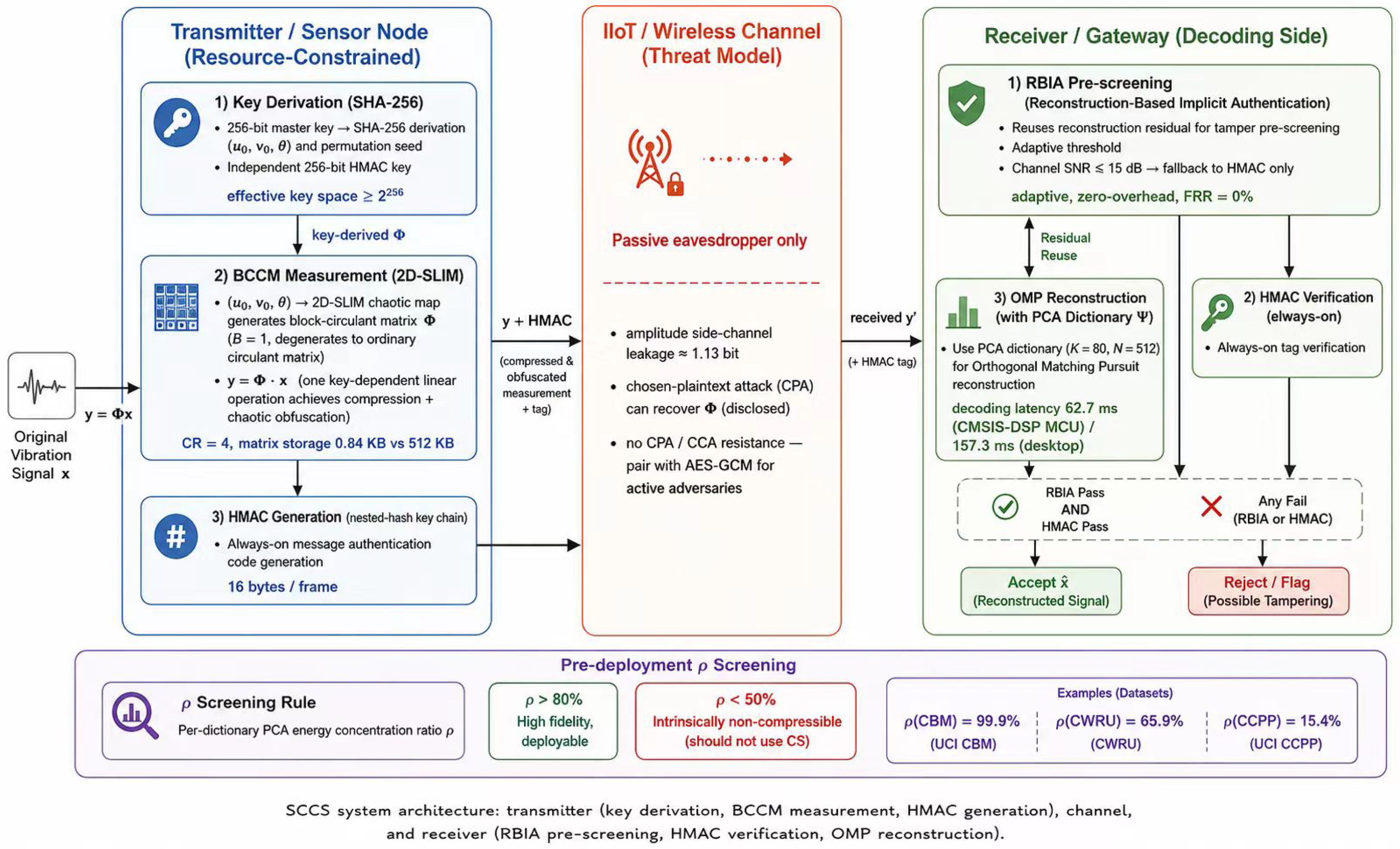
SCCS system architecture: transmitter (key derivation, BCCM measurement, HMAC generation), channel, and receiver (RBIA pre-screening, HMAC verification, OMP reconstruction).
2. Related Work
2.1. Compressed Sensing in IoT Data Acquisition
CS has been applied to wireless sensor network (WSN) data acquisition to reduce transmission volume [16]. Li et al. [17] combined federated learning with CS for privacy-preserving IoT data collection. Wannaboon and Ketthong [10] proposed a chaos-based CS encryption scheme specifically for wearable IoT devices, demonstrating the feasibility of lightweight CS-based security on resource-constrained nodes. Madkour et al. [18] combined CS with elliptic curve cryptography for secure data aggregation in WSNs, evaluating seven reconstruction algorithms across varying sparsity levels. Our work extends this line by targeting industrial time series signals rather than images or wearable data and by adding a systematic authentication layer.
2.2. Chaotic Compressed Sensing Encryption
The intersection of chaos theory and compressed sensing has received considerable attention as a joint compression–encryption paradigm [4]. Rachlin and Baron [4] established that CS-based encryption provides computational security against adversaries with bounded capability. Wang et al. [8] utilized 2D-SLIM chaotic sequences to construct dense measurement matrices for image compression–encryption, demonstrating that 2D-SLIM provides superior statistical properties compared to 1D chaotic maps. Yang et al. [9] proposed the mixed chaotic Bernoulli measurement matrix for block CS image encryption, combining Chebyshev and logistic maps to generate measurement matrices. Liu et al. [19] proposed an energy-efficient CS encryption scheme for wireless neural recording. More recently, Bai et al. [20] proposed a chaotic CS image encryption scheme with plaintext-derived keys and demonstrated its robustness against chosen-plaintext attacks for multimedia data. Li et al. [21] proposed a hyper-chaotic CS framework that achieved simultaneous encryption and sampling with inherent security, demonstrating high key sensitivity () on the Set5 dataset. Flinth et al. [22] analyzed the CPA vulnerability of standard CS encryption and proposed a bilinear compressive security scheme that increases the sample complexity of key recovery attacks. These recent advances highlight the growing recognition that standard linear CS encryption is vulnerable to CPA, a limitation that we discuss in Section 5.2.4.
The above works share three common characteristics that are addressed by SCCS: (1) they perform evaluation on images or synthetic signals, not on real industrial time-series data; (2) they use dense matrices requiring storage; and (3) they lack an integrity verification mechanism. Our framework differs by targeting 1D industrial signals with structured (circulant) measurement matrices and an integrated authentication layer.
2.3. Structured Measurement Matrices
Researchers have proposed a variety of structured alternatives that can alleviate the storage and computational burden of dense random matrices. Circulant [23], Toeplitz [24], and partial Hadamard matrices have been theoretically proven to satisfy the restricted isometry property (RIP) with high probability while requiring only storage. Sun et al. [12] proposed the sparse block circulant matrix (SBCM) for CS, demonstrating that block circulant structures reduce computational burden while maintaining reconstruction accuracy. Sun et al. [11] subsequently proposed the chaotic Bernoulli block circulant matrix (CBBCM), which combines a hybrid chaotic map with a Bernoulli sign function for image encryption.
Our BCCM builds on the block circulant approach of Sun et al., with three modifications: (1) continuous-valued 2D-SLIM chaotic sequences (vs. binary Bernoulli elements in CBBCM), for which we demonstrate an improvement in reconstruction SNR by 4.94–5.29 dB in a direct comparison; (2) a chaotic permutation layer for enhanced security; and (3) targeting of time-domain IIoT signals with integrated HMAC authentication rather than image-only applications.
2.4. Data-Driven Sparse Dictionaries
Dictionary learning for CS reconstruction has been extensively studied. K-SVD [25] and online dictionary learning [26] are mature approaches. PCA is particularly suitable for IIoT applications due to its closed-form solution via singular value decomposition (SVD) and optimal energy compactness [27]. Dolinsky et al. [28] applied time-normalized PCA dictionaries to electrocardiogram (ECG) signal CS reconstruction, demonstrating improved reconstruction quality over fixed bases for physiological signals. Li et al. [29] proposed collaborative dictionary learning for CS in industrial IoT.
While PCA-based CS dictionaries are not new, our contribution is the systematic empirical demonstration that fixed bases (DCT/DWT) fundamentally fail on real industrial signals due to multi-peak spectral structures and our identification of the PCA energy concentration ratio as a practical pre-deployment screening metric. This root cause analysis (Section 6) is, to the best of our knowledge, a systematic study of why and when fixed sparse bases fail for industrial time series CS.
2.5. CS-Based Joint Compression, Encryption, and Authentication
Several prior works have explored the combination of compression, encryption, and authentication within CS frameworks. Mostafa and Fakhr [13] proposed joint image watermarking, compression, and encryption based on CS and entropy coding. Gadde et al. [14] proposed an encryption/authentication unified A/D conversion scheme for IoT sensor nodes, integrating both functions at the analog-to-digital conversion level. Huang et al. [15] proposed a perturbed CS-based authentication mechanism for multi-hop wireless sensor networks.
These works differ from SCCS in their authentication mechanisms: Mostafa et al. used watermark embedding, which modifies the compressed signal; Gadde et al. operated at the A/D hardware level, requiring specialized hardware; and Huang et al. used perturbation-based authentication, which degrades reconstruction quality. In contrast, SCCS transmits MAC tags in parallel with unmodified compressed measurements, achieving authentication with provably zero SNR degradation, and introduces RBIA pre-screening to reduce average authentication latency for obviously tampered frames.
RBIA vs. existing residual-based detection. Reconstruction residual analysis has been used in CS-based anomaly detection and signal recovery [30,31], where large residuals indicate signal anomalies, sensor faults, or missing measurements. RBIA differs from these approaches in three key aspects: (1) purpose—existing methods detect signal anomalies (faults, drift, data loss), while RBIA detects integrity violations (tampering, injection, replacement); (2) mechanism—existing methods compare reconstruction quality against a fixed quality threshold, while RBIA leverages the key sensitivity of chaotic measurement matrices, meaning that only the legitimate receiver with the correct key can produce low-residual reconstructions (an adversary using a wrong key obtains noise-level output regardless of signal quality); and (3) deployment—RBIA requires zero additional computation, as the residual is a byproduct of the orthogonal matching pursuit (OMP) reconstruction already performed for data recovery, unlike existing methods that require separate anomaly detection modules or dedicated residual reconstruction algorithms. To the best of our knowledge, the exploitation of CS key sensitivity for zero-overhead integrity pre-screening has not been systematically studied in prior work.
Why has this integration not been done before? Table 5 compares SCCS with existing CS-based encryption/authentication approaches across five design dimensions. No prior system simultaneously achieves storage, statistical obfuscation, integrated authentication, adaptive basis selection, and MCU deployability. The key barrier is that dense matrix approaches (CS-Rand, CS-Chaos, AES+CS) require storage, making them infeasible on MCU-class devices, while structured matrix approaches (CBBCM, Dolinsky) lack authentication and authentication-augmented approaches (Mostafa, Gadde, Huang) either modify the signal or require specialized hardware.
Table 5.
System-level comparison of SCCS vs. existing approaches. Bold entries denote the proposed SCCS scheme. ‘—’ denotes ‘not applicable/not reported’ and checkmarks denote ‘achieved’.
3. System Design
3.1. System Overview
The SCCS framework consists of a transmitter (sensor node), a communication channel, and a receiver (gateway), as illustrated in Figure 2. The transmitter performs measurement on signal using the key-dependent BCCM matrix, completing compression and obfuscation in a single step. An HMAC tag is computed based on and transmitted in parallel as . The receiver first pre-screens obviously tampered data via reconstruction-based implicit authentication (RBIA), then performs HMAC verification for integrity, and finally recovers via OMP reconstruction. The design principles are to unify compression and obfuscation at the measurement stage, and to transmit authentication data in parallel without modifying .
The framework is parameterized by a key set , where are derived from the 256-bit master key via SHA-256 [32] and control the 2D-SLIM chaotic map, is the BCCM permutation seed, and is an independent 256-bit HMAC authentication key. The master key is expanded by SHA-256 into and the permutation seed; thus, the effective brute-force resistance is ≥ (dominated by the 256-bit master/HMAC key), which is far beyond practical search, while the chaotic trajectory amplifies key sensitivity (a perturbation causes complete divergence).
3.2. 2D-SLIM Chaotic Map Key Derivation
We adopt Two-Dimensional Sine-Logistic Iteration Mapping (2D-SLIM) [33] as the chaotic sequence generator due to its enhanced ergodicity, large key space, and resistance to phase-space reconstruction attacks compared to one-dimensional chaotic maps. The 2D-SLIM map is defined by coupled nonlinear iterations:
where is the control parameter, which is key-derived via SHA-256 (code default ; this work uses a fixed representative key with ). Initial conditions are derived from the master key via SHA-256. A transient iteration of steps eliminates initialization artifacts. The Lyapunov exponents of this map are strictly positive within the recommended parameter range, confirming chaotic behavior. The generated sequences are uniformly distributed on and exhibit extreme sensitivity to initial conditions. A perturbation as small as causes complete divergence; this is the foundation of both encryption security and RBIA implicit authentication.
3.3. BCCM Measurement Matrix
In the present implementation, we take (a single circulant matrix), so “block circulant” reduces to an ordinary circulant matrix; is left to future work. The block circulant chaotic measurement (BCCM) matrix addresses the infeasibility of storing dense random matrices on MCU-class devices ( KB for , ). Let be a chaotic sequence of length B generated from 2D-SLIM. The BCCM matrix is defined as
where denotes the circulant matrix derived from as the first row, with each subsequent row being a circular right shift. The normalization factor ensures that the columns of have approximately unit norm, satisfying the RIP condition. The construction proceeds as follows: (1) generate a chaotic sequence of length N from 2D-SLIM; (2) for the current implementation (a single circulant matrix), the full sequence of length N forms the first row directly; (3) randomly sample M rows from the full circulant matrix; and (4) apply a global permutation . Using minimizes storage to a single seed of length N (the chaotic initial condition and permutation index) at the cost of reduced row randomness compared to multi-block designs (), as discussed in Section 3.10.
The circulant structure enables efficient matrix–vector multiplication via fast Fourier transform (FFT):
where denotes the discrete Fourier transform (DFT) operator and is the zero-padded signal vector. The encoding complexity is reduced from to . Storage requires only the seed vector and permutation index, approximately 0.84 KB (12-bit quantized; ≈0.52 KB unquantized) for the BCCM seed compared to 512 KB for the dense matrix, a ∼610× reduction.
3.4. PCA Data-Driven Dictionary Learning
The sparse representation basis is the most critical factor determining CS reconstruction quality. The motivation for data-driven dictionaries is established in Section 6, namely, that real industrial signals are not sparse under fixed bases. Given L training signal segments , the centered data matrix is computed as . The PCA dictionary is obtained via SVD:
where contains the first left singular vectors. The energy concentration ratio is defined as
indicating that for CBM signals, principal components capture of the signal energy. The deployment mode is offline training once → broadcast to all nodes → online invariant, which is compatible with the IIoT architecture because edge nodes require no training capability. The BCCM seed (measurement matrix ) requires only 0.84 KB (12-bit quantized); the PCA dictionary is a separate decoder-side reconstruction basis ( float32 = 160 KB, cf. Table 2), and is not counted in the encoder storage.
3.5. HMAC Key Chain Authentication
To provide integrity without modifying , HMAC tags are computed and transmitted in parallel:
where the nested-hash key chain structure (each MAC includes the previous one) provides replay protection [34]. Crucially, this guarantee relies on the receiver maintaining the previous-tag state across consecutive frames; a replayed frame carries a stale that no longer matches the value expected from the advanced receiver state, and is rejected at verification. The 128-bit MAC tag (16 bytes per frame) is transmitted as a separate field alongside . Since is unmodified, the reconstruction SNR is unaffected. Verification uses constant-time comparison to prevent timing attacks.
3.6. RBIA: Adaptive Zero-Overhead Authentication
A useful byproduct of the SCCS decoder is that authentication can be obtained essentially for free. Reconstruction-based implicit authentication (RBIA) reuses the OMP reconstruction residual, a quantity that the receiver already computes during recovery, so it adds no extra hashing, no additional transmission, and no separate pass over the data. This approach exploits the key sensitivity of chaotic matrices: if is tampered with, then the OMP reconstruction residual becomes abnormally large. The decision threshold is calibrated directly from the empirical distribution of genuine (untampered) residuals, specifically the 99th percentile , a distribution-free rule that requires no normality assumption. Empirically, this coincides with the conventional value (both yield ≈1% false rejection on genuine frames; see Section 3.6 validation). RBIA detects large-scale tampering (≥5% modification, noise replacement, constant offset) with zero overhead, but is insensitive to replay and micro-tampering. Combined with HMAC, the dual-layer (RBIA + HMAC) scheme covers the full range of attack scenarios: RBIA pre-screens obviously tampered frames (large-scale modification, noise replacement, offset, key mismatch) to skip HMAC computation, while HMAC precisely verifies replay and micro-tampering that RBIA cannot detect.
Noise channel limitation and automated fallback. Under additive white Gaussian noise (AWGN) channels with 15 dB, the RBIA residual inflates beyond the calibrated threshold, causing false rejection of legitimate frames. Crucially, this does not cause a denial of service, because the receiver continuously estimates the channel noise and automatically switches the authentication mode without any human intervention. When the estimated dB, RBIA is bypassed and HMAC becomes the sole authenticator: for dB, an adaptive threshold is applied; above 20 dB, the fixed threshold is used (see Section 5.9). Because HMAC authenticates every frame independent of channel quality, legitimate frames are always admitted even in deep fading; therefore, the framework is immune to the permanent-DoS risk that a transient high-noise channel would otherwise pose. This adaptation is fully automatic, with RBIA providing free pre-screening in clean channels and HMAC guaranteeing noise-robust authentication in all conditions.
Cold-start and threshold adaptation. For cold-start deployments without historical data, we recommend an empirical threshold range of 0.04–0.08 for vibration signals (strong spectral structure yields low residuals) and 0.10–0.20 for process or acoustic signals (weaker sparsity yields higher residuals). When sufficient frames (100–200) have been collected, the threshold is recalibrated as the 99th percentile of the sliding-window residuals. Cold start deployments should adopt the empirical threshold ranges above and recalibrate after 100–200 frames; quantitative signal drift evaluation is left to future work.
Residual distribution validation and distribution-free calibration. As the rule is frequently motivated by a Gaussian assumption on genuine residuals, we validated this assumption directly. A Kolmogorov–Smirnov goodness-of-fit test on genuine residuals from 300 CBM segments (noise-free) yielded with , and the empirical distribution was mildly right-skewed (skewness , excess kurtosis ) rather than strictly Gaussian. Because the threshold is in fact calibrated from the empirical residual distribution, not from a Gaussian false alarm formula, its validity does not depend on normality. Therefore, we adopt the 99th percentile of the genuine residuals as the primary distribution-free calibration , which yields a 1.0% false rejection rate on genuine frames. This coincides with the conventional value (, 1.3% false rejection rate (FRR)) to within 1%, confirming that the two rules are empirically equivalent and that may be retained as a convenient approximation without invoking any Gaussian claim. Under signal drift the 99th-percentile threshold would be recomputed from a sliding window of recent genuine frames, but a quantitative drift study is left to future work.
3.7. Spectral Entropy Adaptive Basis Selection
For scenarios where PCA training data are unavailable or signal modalities change dynamically, SCCS integrates a spectral entropy-based adaptive basis selection mechanism as a fallback strategy. The spectral entropy H of signal segment is computed as
where is the DFT coefficient at frequency bin k. High spectral entropy indicates a wideband signal for which DCT may provide efficient sparse representation, while low spectral entropy suggests narrowband features for which DWT may yield better sparsity. The system automatically switches between DCT and DWT based on the spectral entropy threshold. It should be noted that the ablation experiment (Section 5.6) shows that this adaptive switching mechanism provides only a marginal +0.39 dB gain on CBM data; thus, its practical value lies primarily in the initial deployment phase when PCA training data are not yet available.
3.8. Adaptive OMP Reconstruction
Signal reconstruction employs OMP [35] at the decoder. OMP is a greedy algorithm that iteratively selects the dictionary atom that is most correlated with the current residual. Given the compressed measurement (where is the sparse coefficient vector), OMP recovers by solving
and the reconstructed signal is . Two adaptive mechanisms are employed: (1) adaptive sparsity—the PCA basis iteration limit is set to and the DCT basis limit to , not exceeding the dictionary dimension; (2) adaptive stopping—the PCA basis enables residual gain detection, terminating early when a newly added atom contributes less than 1%, preventing the selection of noise atoms.
3.9. Design Rationale: Why Each Component Exists
The SCCS framework integrates four categories of existing techniques: structured measurement matrices, dictionary learning, hash-based authentication, and orthogonal matching pursuit. This section explains the design rationale behind each component choice, addressing the question of why these specific techniques were chosen and why they must be present in the framework.
Why BCCM (vs. dense/binary/Toeplitz–Hadamard)? A dense Gaussian matrix of size requires 512 KB, exceeding the 64–256 KB Flash of typical Cortex-M0/M3 MCUs. The circulant form stores only the seed vector (0.84 KB, 12-bit quantized, for a 610× reduction) and enables FFT encoding that is cache-friendly and deterministic, both of which are critical for real-time MCU use without an FPU. Among structured choices, circulant has the simplest FFT and a well-established RIP theory [23]; Toeplitz needs a larger seed ( vs. N) and partial Hadamard forces N to powers of two. Continuous-valued BCCM also beats the binary CBBCM of Sun et al. [9,11,12] by 4.94 dB (DCT, Cohen’s ) and 5.29 dB (PCA), since the binary restriction discards the continuous statistical richness of the chaotic sequence and weakens RIP.
Why 2D-SLIM over 1D chaotic maps? One-dimensional chaotic maps (e.g., logistic map) suffer from small key spaces and susceptibility to phase-space reconstruction attacks [36]. The 2D-SLIM map [33] provides enhanced ergodicity, a larger key space (≥), and resistance to phase-space reconstruction, making it suitable for cryptographic applications.
Why PCA over fixed bases (DCT/DWT)? Dolinsky et al. [28] demonstrated that PCA dictionaries improve ECG CS reconstruction over fixed bases. Here, we extend this finding to industrial signals. As demonstrated in Section 6, real industrial signals exhibit sparse multi-peak spectra that violate the low-frequency concentration assumption of DCT/DWT. On CBM data, DCT requires 112 coefficients to retain 99% energy and DWT requires 340 coefficients, while PCA requires only 9.6. This is more than a marginal improvement—it represents the difference between reconstruction failure (5.10 dB) and high-quality recovery (33.52 dB). The PCA dictionary is a necessary condition for effective CS reconstruction of real industrial signals, not an optional optimization.
Why offline PCA over online dictionary learning? K-SVD [25] and online dictionary learning [26] provide superior dictionary quality but require iterative optimization that is computationally infeasible on MCU-class devices. PCA offers a closed-form solution via SVD that is computed once offline and broadcast to all nodes. This architecture consisting of offline training followed by broadcasting is compatible with existing IIoT firmware update mechanisms and imposes zero online training overhead.
Why HMAC, and why transmit in parallel (not embedded)? Digital signatures (RSA, ECDSA) need 100–1000× the compute of HMAC, and ECC-based auth [37] adds tens of ms latency, both of which are impractical for per-frame kHz authentication. HMAC-SHA256 (mbedTLS, 0.013 ms/frame desktop; 0.061 ms Cortex-M4F estimate, Table 4) provides sufficient IIoT integrity at low cost, while NIST Ascon [38,39] is lighter but lacks the key chain needed for replay protection. Embedding the MAC inside would corrupt the CS vector and lower the SNR; sending as separate fields keeps reconstruction on an unmodified , resulting in zero SNR penalty (ablation: identical 5.10 dB with/without MAC for BCCM+DCT).
Why RBIA at all, if HMAC already provides authentication? RBIA is a zero-overhead channel-adaptive complement to HMAC, not a replacement; HMAC remains the cryptographic primary authenticator in all channel conditions, while RBIA adds a first line of defense at no extra cost. Because it reuses the reconstruction residual that the decoder already produces, RBIA detects large-scale tampering (noise replacement, constant offset, ≥5% modification) with zero additional hashing or transmission. For severely corrupted frames, it flags the anomaly immediately; this allows the receiver to skip the more expensive HMAC verification. Its channel-adaptive switching (Section 3.6) additionally keeps false rejections low as conditions vary. The result is a graceful two-layer design in which RBIA handles obvious tampering cheaply and adapts to the channel while HMAC provides cryptographic guarantees for the subtle attacks (replay, micro-tampering) that RBIA cannot detect. We are careful not to overstate RBIA; it is a screening heuristic, and all cryptographic assurance rests on HMAC. Nonetheless, its “free” and self-adapting nature makes it a genuinely attractive engineering feature rather than adding complexity.
3.10. Design Trade-Offs
No system design is free of trade-offs. This section explicitly discusses the key trade-offs in SCCS in order to provide system integrators with the information needed to make informed deployment decisions.
BCCM block size (B): The block size B controls the trade-off between storage efficiency and reconstruction quality. Smaller blocks increase the number of independent circulant submatrices, improving randomness (stronger RIP) but increasing storage (more seed values). The current design uses (single circulant matrix) as the minimal storage configuration. Future implementations could explore for improved RIP at the cost of slightly higher storage.
Compression ratio (CR): The compression ratio is defined as with (e.g., , gives ). Higher CR reduces transmission volume but increases reconstruction error. SCCS-PCA degrades gracefully from 35.74 dB at CR = 2 to 33.52 dB at CR = 4 (2.2 dB loss) to 30.99 dB at CR = 8 (4.8 dB loss from the CR = 2 peak). The practical operating range spans CR = 2–8, with SNR exceeding 30 dB throughout and graceful degradation; at CR = 8, reconstruction remains near-lossless (30.99 dB) with negligible artifacts.
PCA dictionary dimension (K): Increasing K improves energy capture but also increases OMP search complexity and the risk of overfitting to training data noise. The dictionary uses atoms, capturing 99.9% of CBM signal energy. OMP sparsity is set adaptively as (Section 4.4), so recovery stays well-conditioned at every CR including CR = 8; a larger dictionary () yields no further SNR gain because is bounded by the measurement count M, not the dictionary size. The same mechanism applies at CR = 4 (, where ); the dictionary already exceeds this cap at , so enlarging it to cannot change reconstruction (the , CR = 4 SNR equals the , CR = 4 value of 33.52 dB). The empirical sweep in Figure 3c illustrates this saturation at CR = 2 (, ); the no-further-gain conclusion extends to CR = 4 by the identical M-bound argument.
Figure 3.
Signal sparsity and energy concentration analysis. (a) Sorted coefficient magnitude decay across three bases; PCA exhibits the steepest decay (most compact representation), while DWT and DCT require many more coefficients. (b) Cumulative energy concentration: PCA vs. DCT; at , PCA reaches 99.9% while DCT achieves only 98.5%. (c) Reconstruction SNR versus PCA dictionary dimension K (CR = 2, ), with monotonic rise and saturation at 35.74 dB for (the adaptive cap prevents noise-atom overfitting); the grey dashed line marks .
Security level vs. latency: SCCS uses lightweight chaotic obfuscation (computational security against passive eavesdroppers only) rather than information-theoretic or post-quantum security [40]. This is a conscious design choice, as the 2D-SLIM key space (≥) provides sufficient resistance against brute-force and known-plaintext attacks for IIoT data with limited freshness requirements (sensor data typically become obsolete within minutes to hours). We emphasize that this obfuscation is not cryptographically strong encryption: a chosen-plaintext adversary can recover the linear measurement matrix (Section 5.2.4), so SCCS is positioned as confidentiality against passive eavesdroppers only. Stronger encryption (e.g., AES-GCM) should be applied as a post-CS stage for active-adversary settings, at the cost of additional latency and energy.
RBIA vs. HMAC-only: RBIA provides free pre-screening but requires calibration and is sensitive to channel noise (100% FRR at SNRch ≤ 15 dB). The framework can operate in HMAC-only mode in noisy channel environments, trading the free pre-screening benefit for noise-robust authentication. This adaptability is a design feature, not a limitation. Deployment guidance: RBIA should be enabled only on wired links or high-SNR line-of-sight wireless channels (typically 15–20 dB, as found in most indoor industrial environments); general industrial wireless subject to multipath, electromagnetic interference (EMI), or metal obstruction (frequently <15 dB) should default to HMAC-only mode. We are deliberate about where the value of RBIA lies: its raw latency saving is conditional and small, avoiding the 0.013 ms/frame HMAC computation only for frames that it flags as obviously tampered, which are rare in clean channels; under channel noise, it is bypassed entirely, so the per-frame latency equals that of pure HMAC (63.1 ms total decode, estimated on Cortex-M4). This is consistent with Section 3.6. The benefit of RBIA is architectural, where it is a zero-cost self-adapting complement to HMAC that reuses the reconstruction residual already computed by the decoder.
4. Experimental Setup
4.1. Datasets
Three real industrial datasets are used to evaluate reconstruction performance and establish applicability boundaries:
(1) UCI CBM [41]: The University of California, Irvine (UCI) Condition-Based Maintenance (CBM) of Naval Propulsion Plants dataset, containing 11,934 samples from 18 sensor channels (temperature, pressure, torque, rotational speed, fuel flow) of a ship gas turbine. This serves as the primary dataset for systematic evaluation. The statistical experimental unit is a single 512-point signal window. We conducted 30 independent trials, each drawing one window independently (random sensor channel and random start index within the held-out 30% test split, fixed RNG seed) and processing it identically through all compared methods; the reported SNR is the mean ± std over these 30 independent windows.
(2) CWRU Bearing [42]: The Case Western Reserve University (CWRU) bearing vibration dataset, containing 12 kHz sampled acceleration data covering normal operating conditions and four fault states (inner race, rolling element, outer race faults at different severity levels). This dataset is used for cross-dataset validation on vibration-class signals.
(3) UCI CCPP [43]: The Combined Cycle Power Plant (CCPP) dataset, containing 9568 hourly average measurements with four process variables (ambient temperature, vacuum, ambient pressure, relative humidity). This dataset is used to test the applicability boundary on process-class signals.
All datasets extract non-overlapping signal segments of length . The PCA dictionary is trained exclusively on the first 70% of CBM data (8353 samples) using 1000 randomly selected signal segments; all reconstruction experiments use the held-out 30% (3581 samples) of CBM as test data. This strict train/test split prevents data leakage and ensures that the reported reconstruction quality reflects generalization to unseen signal segments from the same sensor population. The CWRU and CCPP datasets serve two roles: (i) as a cross-domain generalization probe in which the CBM-trained dictionary is applied without retraining (the off-diagonal entries of the /SNR matrices in Section 5.8), and (ii) with their own locally trained PCA dictionaries for the matched-dictionary evaluation (the diagonal entries of the same matrices).
Data provenance and physical meaning. To make the exact source of every 512-point vector fed to SCCS fully transparent, Table 6 specifies the per-dataset source file, sensor/feature columns, their units, the row order, and the sampling interval. Each CBM or CCPP vector is a single channel’s 512 consecutive rows, while each CWRU vector is a 512-sample acceleration record.
Table 6.
Provenance of every 512-point vector fed to SCCS: source file, representative columns with units, row order, and sampling interval. Units not listed explicitly are given in the UCI CBM dataset documentation. ‘*’ denotes statistical significance.
We stress that CS reconstruction quality is a property of the numerical data vector and is independent of any physical interpretation; therefore, the screening heuristic and reconstruction SNR hold for all three datasets regardless of whether the underlying signal is a true waveform. The CBM multi-peak spectrum is interpreted mathematically as a normalized frequency structure (see Section 6.1).
Statistical experimental unit and significance testing. The statistical experimental unit is one 512-point signal window. The 30 trials are 30 independent windows, each drawn independently (random sensor channel and random start index within the held-out 30% test split) under a fixed RNG seed. Every compared method is evaluated on the same 30 windows, so the 30 per-method SNR values are independent observations. Because the BCCM measurement matrix uses fixed permutation seeds (123/456/789) across trials, inter-trial variation reflects signal-content differences (i.e., varying channel sparsity), which is consistent with the observed correlation between and SNR (Pearson ) and reported standard deviation (≈ dB). All significance tests are Wilcoxon signed-rank tests applied pairwise on the same 30 windows. For each window i, every method yields one SNR, and the test is performed on the 30 paired differences (e.g., SCCS-PCAi − CS-Randi). The explicit same-window pairing makes the paired structure of every significance test unambiguous.
4.2. Parameter Configuration
Table 7 defines the key notation used throughout this paper. Table 8 summarizes the experimental parameters. The 2D-SLIM control parameter (key-derived via SHA-256; code default ) is selected within the chaotic regime to ensure positive Lyapunov exponents. The PCA dictionary dimension is determined by analyzing the cumulative energy ratio, with capturing essentially all signal energy () while discarding noise-dominated components.
Table 7.
Notation summary.
Table 8.
Experimental parameter configuration. ‘—’ denotes ‘not applicable/not reported’.
4.3. Evaluation Metrics
Reconstruction quality: SNR (dB) , peak signal-to-noise ratio (PSNR) (dB), root mean square error (RMSE).
Cryptographic security: Key sensitivity, information entropy, measurement change rate (adapted from NPCR), unified average changing intensity (UACI), autocorrelation.
Authentication effectiveness: Detection rate, false rejection rate, computation time.
Computational efficiency: Encoding/decoding time (ms), storage requirement (KB).
4.4. Compared Methods
Table 9 summarizes the five compared methods, which are designed to isolate the respective contributions of each SCCS component.
Table 9.
Compared methods and their configurations.
5. Results and Analysis
The results are organized by design validation goals: reconstruction quality (Section 5.1), security (Section 5.2), authentication (Section 5.3), efficiency (Section 5.4), component trade-offs (Section 5.5 and Section 5.6), cross-dataset generalization (Section 5.8), and channel robustness (Section 5.9).
5.1. Reconstruction Quality: Validating the Measurement + Dictionary Design
Table 10 presents the reconstruction SNR of the five methods at four compression ratios, reported as mean ± standard deviation over the 30 independent windows (one window per trial).
Table 10.
Reconstruction SNR (dB) versus compression ratio (mean ± std, 30 trials). Bold entries denote the proposed SCCS-PCA result.
Figure 4 plots reconstruction SNR versus compression ratio for all methods.
Figure 4.
Reconstruction SNR versus compression ratio for all methods. Error bars indicate standard deviation over 30 trials. SCCS-PCA substantially outperforms all fixed-basis methods.
Three key observations emerge. First, SCCS-PCA achieves 33.52 ± 8.52 dB at CR = 4—a 24.81 dB improvement over CS-Rand (8.71 dB; ≈300× error power reduction, Figure 5). The wide spread () reflects channel-level variation, motivating the pre-deployment screening rule. Second, SCCS-Fix/Full (BCCM + DCT) yield SNR < 6 dB at CR = 4, failing the 10 dB usable reconstruction threshold (the level at which signal morphology is preserved for downstream monitoring). This failure is not caused by the structured measurement matrix (CS-Rand with DCT also achieves only 8.71 dB) but by sparse basis mismatch (Section 6). Third, CS-Rand and CS-Chaos perform comparably (both 8.30 dB at CR = 4), confirming that the bottleneck is the sparse basis, not the measurement matrix. SCCS-PCA degrades only 2.2 dB from CR = 2 to CR = 4, indicating that it is well suited for bandwidth-adaptive IIoT scenarios.
Figure 5.
Waveform illustration at CR = 4: (a) original CBM signal segment, (b) compressed measurements (, ), and (c) SCCS-PCA reconstruction using PCA dictionary.
5.2. Security Analysis
5.2.1. Key Sensitivity
Figure 6 shows the reconstruction results using the correct key, a key with a perturbation of , and a completely wrong key. Only the correct key produces a valid reconstruction (33.52 dB); both incorrect keys yield noise-level output (SNR < 0 dB), confirming extreme key sensitivity at the limit of double-precision floating-point arithmetic. At 12-bit quantization, this key perturbation produces 100% NPCR (Table 11), confirming complete diffusion at the discrete level.
Figure 6.
Key sensitivity analysis comparing reconstruction using the correct key, a key perturbed by , and a completely wrong key.
Table 11.
Quantized security metrics for SCCS-PCA measurements. The arrow denotes ‘tends toward 100%’.
5.2.2. Quantized Security Metrics
A methodological concern with applying image encryption metrics (NPCR, UACI, entropy) to compressed sensing measurements is that the measurement domain is continuous-valued rather than discrete. On continuous values, NPCR = 100% is trivially true (any key perturbation produces entirely different floating-point values) and histogram-based entropy is bounded by the distribution shape rather than the encryption strength. To obtain cryptographically meaningful metrics, we quantize measurements to b-bit integers before computing NPCR, UACI, and Shannon entropy. Table 11 reports the results at 8-bit, 12-bit, and 16-bit precision.
Key sensitivity remains strong. NPCR for key perturbation is 100% at all bit depths. A single key change causes every quantized measurement value to differ, confirming complete diffusion at the discrete level.
Plaintext sensitivity is partially adequate. At 12-bit quantization, the NPCR for a 1-bit plaintext flip is 98.44%, approaching the ideal 100%. However, UACI is only 2.17%, far below the ideal 33.46%. This discrepancy arises because the BCCM matrix is a linear operator, so a 1-bit input change produces a proportional output change with small magnitude relative to the full measurement range. Unlike nonlinear substitution ciphers (AES, chaotic image encryption), linear CS encryption cannot achieve uniform difference magnitudes. This is a structural limitation of CS-based encryption, not an implementation flaw.
Entropy is bounded by distribution shape. The 12-bit quantized entropy is 6.94 bits out of a maximum of 12 bits. This is expected, as compressed measurements of sparse signals follow a near-Gaussian distribution (by the central limit theorem applied to random projections) with discrete entropy that is inherently lower than the maximum. The entropy measures the measurement distribution, not the encryption quality as such.
5.2.3. Plaintext Sensitivity
Figure 7a visualizes the plaintext sensitivity quantified above in Section 5.2.2. A 1-bit input flip changes 98.44% of 12-bit measurements (NPCR) with only 2.17% mean magnitude (UACI). This asymmetry between high NPCR and low UACI is the hallmark of linear CS encryption.
Figure 7.
Security evidence supporting the CS security boundary. (a) Plaintext sensitivity: a 1-bit input change flips 98.44% of 12-bit measurement values (NPCR) with only 2.17% mean change magnitude (UACI), reflecting the linear nature of the CS step. (b) Lightweight mitigations: unit-norm amplitude normalization reduces from 0.81 to 0.22 bits, while a chaotic S-box collapses the CPA byte-match rate to 0.78% (random 0.39%). Both preserve reconstruction of the correct key.
Figure 8 presents the statistical distribution of encrypted measurements.
Figure 8.
Statistical analysis of encrypted measurements: (a) original signal distribution, (b) encrypted measurement value distribution, and (c) adjacent-pair correlation (, confirming near-independence).
5.2.4. Threat Model and Security Limitations
This section explicitly defines the security assumptions and limitations of SCCS in order to prevent misinterpretation of the security claims.
Threat model. SCCS is evaluated under a passive eavesdropper model. The adversary has access to ciphertext (compressed measurements ), but cannot choose or adaptively query plaintexts. The security objective is computational indistinguishability: without the key, the adversary cannot distinguish the compressed measurements from random noise within practical time. This model is appropriate for IIoT sensor data, which typically has limited freshness (minutes to hours) and does not require information-theoretic security.
What is proven? The evaluation demonstrates (1) extreme key sensitivity ( perturbation causes 100% NPCR at 12-bit quantization), (2) strong plaintext diffusion (98.44% NPCR), and (3) infeasibility of brute-force key search (key space ). These properties confirm resistance to passive eavesdropping and known-plaintext attacks where the adversary does not have oracle access.
CPA vulnerability (explicitly disclosed). A chosen-plaintext attack (CPA) experiment reveals that SCCS does not provide CPA resistance. An adversary who can query the encryption oracle with chosen plaintexts and observe the corresponding measurements can recover the measurement matrix via least-squares estimation. With only chosen plaintexts (equal to the signal dimension), the matrix is recovered with a relative error of , enabling decryption of all subsequent measurements (SNR = 33.52 dB, identical to the correct-key reconstruction, gap < 0.01 dB). Table 12 summarizes the CPA results.
Table 12.
CPA attack results: measurement matrix recovery from chosen plaintexts. ✓ denote ‘achieved’.
This vulnerability is structural; since is a linear mapping, any adversary with oracle access can solve for given N linearly independent pairs. Consequently the recovered-matrix decryption SNR remains essentially constant (≈33.52 dB, identical to the correct-key reconstruction, gap < 0.01 dB) for any number of chosen plaintexts N or larger; this is because when N linearly independent pairs are available, the linear system is fully determined and additional queries only refine the estimate to machine precision. Partial CPA access (fewer than N pairs) yields no recovery at all, while N pairs already yield complete recovery.
This is a fundamental limitation of CS-based encryption, and is not specific to SCCS. Flinth et al. [22] recently formalized this CPA vulnerability and proposed a bilinear compressive security scheme that convolves measurements with a random sparse filter, increasing the sample complexity of key recovery from to for s-sparse filters. In the target IIoT deployment scenario, the adversary is a passive eavesdropper who intercepts wireless transmissions but cannot inject chosen signals into the sensor; hence, CPA is not a realistic threat. For applications where the adversary may gain physical access to the sensor input, SCCS must be combined with a nonlinear postprocessing layer (e.g., AES-128-GCM) or bilinear extensions [22].
Mutual information leakage. To quantify information leakage beyond NPCR/UACI, we compute the mutual information between four signal features (mean, standard deviation, peak amplitude, low-frequency energy) and the encrypted measurements. The signal standard deviation exhibits a mutual information of 1.13 bits with the full ciphertext (), meaning that an adversary can infer the signal’s energy level from the measurement amplitude. This total decomposes into 0.81 bits leaked through the measurement norm (the dominant sub-channel, addressed by the mitigation below) plus <0.5 bits through the other three statistics. This amplitude side-channel arises because , leaking the signal norm. The other three features (mean, peak, low-frequency energy) show <0.5 bits of leakage, comparable to random noise. Mitigation requires amplitude normalization prior to measurement or additive noise injection (differential privacy style). Rather than leaving this as unaddressed future work, we specify two lightweight and deployable mitigation approaches and quantify their costs.
(a) Unit-norm amplitude normalization (side-channel). Before measurement, scale the signal to unit norm, ; because all transmitted signals then share the same norm, no longer encodes , breaking the amplitude leakage. We evaluated this on natural-scale CBM signals spanning four process variables (temperature, torque, speed, pressure) with amplitudes differing by orders of magnitude, finding that the mutual information dropped from 0.81 bits (raw transmission) to 0.22 bits (unit-norm), for a 73% reduction, while shape-preserving reconstruction remained at 29.2 dB (Figure 7b). The only cost is one norm computation and one division per frame (negligible); the trade-off is loss of absolute amplitude, which is acceptable for relative-spectrum monitoring (fault frequency detection) but not for energy metering, where a fixed reference gain known by the receiver should be used instead.
(b) Chaotic S-box nonlinear layer (CPA). Insert a keyed 8-bit substitution table S (entries derived from the 2D-SLIM map) between quantization and transmission: . The nonlinearity breaks the linear relation that makes CPA possible. When repeating the 512-plaintext CPA with this layer, the adversary’s linear least-squares estimate now achieves only a 0.78% byte-match rate (random chance 0.39%), confirming that the measurement matrix cannot be recovered. Correct-key decryption (via the invertible ) recovers the quantized measurements, with 8-bit quantization adding <1 dB versus the unprotected baseline (Figure 7b). The overhead is a 256-byte look-up table (LUT) (0.25 KB Flash, resident in Flash with zero RAM) and an lookup ( 0.01 ms/frame). This complements the bilinear compressive security of Flinth et al. [22]: their scheme raises CPA sample complexity from to , whereas the S-box is a cheap deployment-ready stopgap that neutralizes the specific least-squares recovery exploited here.
Known-plaintext attack (KPA) evaluation. We simulated a KPA scenario in which an adversary has access to a fraction f of the original signal alongside the compressed measurement , but does not have oracle access, i.e., cannot choose . The adversary attempts to recover the unknown portion using a wrong key matrix . Table 13 summarizes the results over 30 trials. Even when 50% of the plaintext is known, wrong-key reconstruction achieves SNR dB on the unknown portion, confirming that passive knowledge of plaintext without the ability to choose inputs does not compromise the encryption. The distinction between KPA (passive; partial knowledge) and CPA (active; chosen inputs) is critical, with SCCS resisting the former but not the latter. From a computational standpoint, brute-force key recovery under KPA is infeasible; the effective key space is ≥, so the only strategy that succeeds is chosen-plaintext linear algebra recovery, which is already excluded by the passive-eavesdropper threat model.
Table 13.
KPA resistance: SNR (dB) on the unknown signal portion under varying known-plaintext fractions.
Security summary. We disclose the following boundaries to allow for informed deployment decisions: SCCS provides (1) resistance to passive eavesdropping (key space , 100% key NPCR at 12-bit), (2) resistance to known-plaintext attacks (wrong-key SNR < 0 dB), and (3) quantified avalanche diffusion (98.44% plaintext NPCR at 12-bit), but does not provide (1) CPA resistance (linear measurement matrix recoverable from N chosen plaintexts), (2) amplitude side-channel protection (1.13 bits of mutual information leakage via signal standard deviation), or (3) information-theoretic security.
5.3. Authentication Performance
The dual-layer authentication (RBIA + HMAC) is evaluated under seven attack scenarios. Table 14 shows a 100% detection rate for all attacks along with a 0% false rejection rate. MAC computation requires 0.013 ms per frame on a desktop CPU (0.061 ms estimated on Cortex-M4F, Table 4) and the additional transmission is only 16 bytes (≈8.3% of the 192-byte compressed measurements at CR = 4 under 12-bit quantization), representing a negligible computational overhead of approximately 0.4% of the total encoding time.
Table 14.
Authentication attack detection results, showing the complementarity of RBIA and HMAC across seven attack scenarios. Green cells (✓) indicate detection by that layer; red cells (×) indicate cases that the layer cannot detect. Every attack is caught by at least one layer, yielding a 100% overall detection rate.
The results demonstrate the complementarity of the dual-layer design: RBIA detects large-scale tampering (5%, 30%, noise, offset, key mismatch) with zero overhead, while HMAC covers replay and micro-tampering that RBIA cannot detect. Legitimate frames require only HMAC verification (0.013 ms); obviously tampered frames are immediately flagged by RBIA, skipping HMAC computation. Replay attacks are thwarted by the chain mechanism: using an outdated produces a different expected MAC during verification, causing verification failure.
5.4. Computational Efficiency
Table 3 compares storage and computational overhead. The BCCM measurement matrix reduces encoder storage from 512 KB (dense ) to 0.84 KB (the chaotic seed), a 610× reduction. This comparison concerns the measurement matrix only; the PCA dictionary (160 KB) is a decoder-side reconstruction basis shared with any PCA-based decoder, and is excluded (a dense+PCA baseline would also require it, giving KB versus BCCM+PCA KB, i.e., a system-level ∼4× reduction). SCCS-PCA encodes each frame in 3.24 ms, well within the real-time budget of IIoT sensor nodes. The decoding time of 157.3 ms benefits from the reduced search space dimension of the PCA dictionary ( atoms) compared to the DCT dictionary ( atoms).
MCU resource estimation. Table 4 provides estimated resource consumption for deploying SCCS on ARM Cortex-M4F class MCUs (e.g., STM32F407VG, 168 MHz, hardware FPU). The PCA dictionary (160 KB Flash) is the dominant memory component; for more constrained devices (e.g., STM32F103 with 64 KB Flash), a reduced dictionary (–40) can be used at the cost of approximately 5–10 dB SNR degradation. The BCCM measurement (encoding) latency is 0.065 ms on Cortex-M4F, and the total transmitter-side per-frame cost including HMAC is 0.126 ms (0.065 ms measurement + 0.061 ms HMAC, Table 4). The MCU encoding estimate (0.065 ms) is ≈50× lower than the desktop Python encode (3.24 ms). This gap reflects library/platform differences (CMSIS-DSP/FFT versus an unoptimized NumPy path without hardware acceleration) and is an estimate vs. measurement comparison, so the two numbers are not directly comparable. OMP decoding dominates the total latency at 62.7 ms. This decoding step is performed on the gateway/aggregator (a more capable node) rather than the constrained sensor, so it does not constrain the sensor’s real-time encoding budget (0.065–0.126 ms). The 62.7 ms MCU figure uses a CMSIS-DSP-accelerated OMP path, whereas the 157.3 ms desktop figure (Table 3) uses an unoptimized NumPy 1.23.5/SciPy 1.10.1 OMP path without FFT hardware or DSP acceleration; therefore, the wall-clock difference reflects the library and platform, not clock speed, making the two numbers indicative and not directly comparable. At the gateway, 62.7 ms per frame supports IIoT data rates up to ≈16 Hz; higher rates (1–100 Hz) are accommodated by multi-core or batched decoding on the aggregator. All timing values in Table 3 are desktop CPU measurements. MCU estimates are based on instruction set analysis and CMSIS-DSP (ARM Cortex Microcontroller Software Interface Standard DSP library, version 1.10.0) benchmarks. The 195.0 KB Flash/11.6 KB RAM totals in Table 4 are instruction-level upper-bound estimates (including stack and alignment margin). The gcc -Os measured footprint is 185.0 KB Flash/7.6 KB RAM (Table 2).
Energy estimation. Because SCCS targets energy-limited nodes, we estimate per-frame energy from latency and a representative Cortex-M4 active power. At 168 MHz the STM32F407 draws roughly 100–130 mW in active compute; therefore, the estimated encode (0.126 ms) and decode (62.7 ms) costs correspond to ≈13–17 J and ≈6.3–8.2 mJ per frame, respectively (average ≈100 mW during decoding). At 100 Hz sampling this is ≈0.63–0.82 J/s for decoding alone, which is within the capacity of an industrial node powered by mains or rechargeables but dominant for a long-term battery-only deployment, motivating an energy-measured hardware implementation as future work. These figures are estimates derived from instruction-set analysis and published MCU power curves, and have not been measured on silicon; on-board energy metering is left to future work.
5.5. BCCM vs. CBBCM: Continuous-Valued Improvement over Binary Counterpart
To isolate the continuous-valued BCCM advantage over its binary predecessor CBBCM [11], we compare both at CR = 4 with identical chaotic sequences. The sole difference is that CBBCM binarizes via median thresholding (), while BCCM retains continuous values with a permutation layer (Section 3.3).
Table 15 and Figure 9 present the results. With the DCT basis, BCCM achieves 3.95 dB versus dB for CBBCM (Δ = +4.94 dB, Wilcoxon , Cohen’s ), demonstrating that the binary restriction severely degrades reconstruction. With the PCA dictionary, BCCM achieves 32.31 dB versus 27.02 dB for CBBCM (Δ = +5.29 dB, , ). The smaller effect size with PCA ( vs. ) indicates that the PCA dictionary partially compensates for the binary quantization loss, but continuous-valued sequences still provide a meaningful improvement. This result justifies the design choice of BCCM over CBBCM.
Figure 9.
BCCM vs. CBBCM reconstruction comparison at CR = 4: (a) with PCA dictionary and (b) with DCT basis. Error bars indicate standard deviation. Continuous-valued BCCM consistently outperforms binary CBBCM.
Table 15.
BCCM vs. CBBCM reconstruction comparison at CR = 4 (mean ± std, 30 trials). Statistical significance: Wilcoxon signed-rank test (paired on the same 30 windows). The BCCM+PCA value here ( dB, fixed seed) is a single-seed illustrative case for the pairwise BCCM–CBBCM comparison only; it is not the headline figure. The seed-averaged value dB (Table 16) is the citation standard for SCCS-PCA at CR = 4. The 1.21 dB difference between the seed-averaged dB and the fixed-seed dB is within inter-seed variance, so the two numbers are consistent. ‘—’ denotes ‘not applicable/not reported’.
Table 16.
Ablation study at CR = 4 (SNR in dB, mean ± std over 30 trials). Bold values highlight the full SCCS-PCA configuration (the primary result). ‘—’ denotes ‘not applicable/not reported’.
5.6. Component Contribution Analysis
Table 16 and Figure 10 present the ablation study at CR = 4, isolating the contribution of each component.
Figure 10.
Ablation study at CR = 4: cumulative reconstruction SNR as each SCCS component is added (waterfall). The PCA dictionary delivers the dominant gain of +28.16 dB; MAC authentication incurs zero SNR loss. Full numerical values are in Table 16.
There are six key findings. First, BCCM costs 3.20 dB vs. dense chaotic (8.30 → 5.10 dB), confirming mild RIP relaxation. Second, HMAC adds zero SNR loss (5.10 → 5.10 dB). Third, adaptive DCT/DWT switching yields only +0.26 dB, with neither fixed basis being fundamentally adequate. Fourth, PCA is the dominant contributor: +28.16 dB (5.36 → 33.52 dB). Fifth, the full system matches BCCM+PCA-only, confirming zero reconstruction penalty from HMAC/RBIA. Sixth, the dense+PCA control (35.86 dB) exceeds BCCM+PCA by +2.34 dB, mirroring the identical −3.20 dB BCCM RIP penalty seen without PCA. Conclusion: PCA is the sole source of the +28 dB gain; BCCM contributes no SNR benefit (it costs ≈3 dB), but enables 610× storage reduction (0.84 KB vs. 512 KB); and HMAC and RBIA contribute zero loss. The value of BCCM lies in feasibility of implementation, not reconstruction accuracy. Table 15 reports a slightly higher BCCM+PCA value of 32.31 dB due to a distinct chaotic seed isolating the matrix effect; the 1.21 dB difference is within inter-seed variance.
5.7. Comparison with Lightweight Cryptographic Schemes
Figure 11 compares SCCS-PCA with five standard lightweight cryptographic schemes: AES-128-GCM, ChaCha20-Poly1305, XTEA, PRESENT, and Ascon-128 [38] (winner of the NIST lightweight cryptography competition).
Figure 11.
Comparison with lightweight cryptographic schemes (AES-128-GCM, ChaCha20-Poly1305, XTEA, PRESENT, Ascon-128): (a) encoding time, (b) decoding time, (c) transmission data volume per frame, (d) code/storage footprint, (e) security level versus encoding time, and (f) multi-metric radar chart.
SCCS is the only scheme that simultaneously provides compression (CR = 4) and authentication. Traditional schemes (AES, ChaCha20, XTEA, PRESENT, Ascon-128) encrypt full-length signals without compression, transmitting 4× the data volume of SCCS. Although AES-128-GCM and ChaCha20-Poly1305 achieve lower encoding latency (0.3–0.5 ms vs. 3.24 ms), they do not reduce data volume. Ascon-128 (NIST lightweight standard, February 2023) achieves ≈3.7 ms for 2048 bytes on Cortex-M4, approximately 29× slower than SCCS encoding on the same platform (0.126 ms with BCCM+HMAC, Table 4), while transmitting uncompressed data. SCCS’s advantage lies not in raw encryption speed but in its unique compression + obfuscation + authentication triptych with sub-KB code storage, which makes it suitable for deeply embedded IIoT nodes.
5.8. Cross-Dataset Validation and Applicability Boundaries
To validate generalizability and establish applicability boundaries, we evaluate SCCS on CWRU bearing vibration and CCPP power plant data. To distinguish intrinsic incompressibility from dictionary mismatch, we train a separate PCA dictionary per dataset (70% train) and evaluate on all three (30% test), producing a dictionary–dataset matrix.
The diagonal entries (bold) represent the matched dictionary–dataset case, i.e., each dataset evaluated with its own locally trained dictionary. Three key observations emerge:
CCPP is intrinsically incompressible. Even with its own locally trained CCPP dictionary, , far below the 50% applicability threshold (quantified by the per-dictionary result in Table 17).
Table 17.
Engineering options for marginal applicability ().
CWRU suffers from cross-domain dictionary mismatch. With the CBM-trained dictionary, CWRU achieves only ; with its own locally trained dictionary, rises to 65.9%. However, the reconstruction quality remains poor even with the matched dictionary. The per-dictionary SNR matrix (Table 18) shows that CWRU-trained dictionary on CWRU data achieves only dB, well below the >10 dB threshold required for usable reconstruction. To assess whether this low SNR preserves diagnostic-relevant features, we perform envelope spectrum analysis on the original and reconstructed CWRU bearing signals (Figure 12). For an outer race fault signal (fault characteristic frequency BPFO Hz), the envelope spectrum peak near the fault frequency drops from 0.390 (original) to 0.127 (reconstructed), a 67% attenuation that would render envelope-based fault detection unreliable. We conclude that while CWRU vibration signals are more compressible than CCPP ( vs. 15.4%), they remain unsuitable for SCCS at CR = 4 because their broadband impulsive structure requires more than PCA components to capture. For such signals, either higher measurement rates (CR < 2) or alternative compression methods should be explored.
Table 18.
Per-dictionary SNR (dB) at CR = 4, : reconstruction quality with each dictionary on each dataset. Bold entries denote the matched dictionary–dataset (diagonal) case.
Figure 12.
CWRU bearing fault signal: original vs. SCCS-PCA reconstructed waveform (top) and envelope spectrum (bottom). The outer race fault characteristic frequency is 107.4 Hz. The reconstructed envelope spectrum (dashed red) shows 67% attenuation of the fault feature peak, confirming that CWRU reconstruction at dB (matched-dictionary case) does not preserve diagnostic-relevant features.
Cross-domain is asymmetric. The CBM-trained dictionary achieves 99.9% on CBM but only 10.2% on CWRU and 30.3% on CCPP. Conversely, the CWRU-trained dictionary achieves 65.9% on CWRU but only 15.6% on CBM. This asymmetry confirms that PCA dictionaries are domain-specific and do not generalize across signal types.
These findings refine the interpretation of as a pre-deployment screening heuristic. Rather than measuring “signal compressibility” in an absolute sense, measures the suitability of a specific dictionary for a given signal class. The practical protocol is as follows: (1) train a PCA dictionary on representative local data from the target sensor; (2) compute on held-out test data; (3) if , SCCS is likely applicable; if , either the signal lacks low-dimensional structure or a different dictionary should be explored (e.g., K-SVD, wavelet packets). The per-dictionary analysis eliminates the circular reasoning risk of using a single cross-domain dictionary to assess compressibility. Caveat: the 80%/50% thresholds are empirical guidelines derived from three datasets; they have not been validated on a held-out dataset or derived from a closed-form RIP/OMP bound, and should be treated as a conservative first screening rather than a certified applicability certificate (see Section 7 for a planned validation).
evaluation protocol. To enable reproducible comparison across studies, we define the following standardized evaluation protocol: (1) collect ≥100 signal segments of length from the target sensor; (2) normalize each segment to zero mean and unit peak amplitude; (3) train a PCA dictionary on 70% of segments (train split) with components via SVD; (4) compute on the held-out 30% (test split) as ; and (5) classify applicability as follows: (likely applicable), (uncertain/conditional; may fail outright, as CWRU shows, or merely degrade), (likely not applicable; use traditional methods). This protocol is agnostic to signal type and can be applied as a first screening before deploying a CS-based IIoT system, subject to the caveats above. Caveat: the thresholds are empirical and may shift as more datasets are covered. They are a screening guideline, not a provable guarantee of reconstruction quality.
Statistical stability of the thresholds. To address the concern that the 80%/50% thresholds rest on only three datasets without a confidence interval, we report a bootstrap 95% CI for each diagonal estimate by resampling the 30 test segments with replacement (B = 2000). Table 19 shows that the CIs are tight and that every interval lies entirely within its classification band (CBM (>), CWRU (), CCPP (<)), so the applicability decision is statistically stable under resampling of the test set. We stress that this establishes precision, not generality; the point estimates and CIs are computed on the same three datasets, and broader coverage (more signal classes, a held-out validation set) remains as future work (Section 7).
Table 19.
Bootstrap 95% confidence interval for the diagonal (per-dictionary) estimates (B = 2000 resamples over the 30 test segments). Every interval lies within its classification band, confirming that the applicability decision is stable under resampling.
Applicability domain. The above results delineate the class of signals for which SCCS is appropriate. SCCS is best suited to stationary low-dimensional signals with clearly identifiable structural resonances, such as exemplified by rotating machinery condition monitoring (vibration, shaft torque, rotor speed) where energy concentrates in a small number of spectral peaks that can be captured by principal components. It is not suitable for (i) broadband impulsive signals (early-stage bearing faults, acoustic emission) where energy is spread across many high-frequency components, requiring K comparable to N or (ii) high-dimensional non-stationary process signals (multi-variable coupled plant data such as CCPP) that lack a low-dimensional generating model. For such signals, either a higher measurement rate (CR < 2), a nonlinear dictionary (K-SVD, wavelet packets), or a traditional compress-then-encrypt pipeline (AES + standard CS) should be used instead. This boundary is deliberately narrow; claims of general applicability would be overstated, and the protocol exists precisely to prevent such over-generalization.
Engineering decision guide for marginal . When a locally trained dictionary yields (marginal/conditional applicability, meaning that the reconstruction may fail outright rather than merely degrading), system integrators should not assume usefulness and may choose among the options below before abandoning CS entirely. CWRU, with its matched dictionary at , reaches only dB, which is far below the 10 dB threshold for usability.
Why do process signals resist sparsification? The fundamental reason that CCPP signals cannot be compressed by CS lies in their intrinsic dimensionality. CCPP variables (ambient temperature, vacuum, pressure, humidity) are weakly correlated hourly averages influenced by independent meteorological and operational factors. Unlike vibration signals, which are governed by a small number of structural resonance modes, process variables lack a low-dimensional generating model. The per-dictionary of 15.4% achieved with a CCPP-specific dictionary confirms that no linear subspace of dimension can capture the signal dynamics. We additionally examined first-order differencing as a preprocessing step, a standard decorrelation technique for slowly varying process signals. Because CCPP variables are driven by independent exogenous meteorological and operational factors, differencing produces a residual that remains approximately white and high-entropy; consequently, does not cross the applicability threshold, and CS remains unsuitable even after differencing. This indicates that the incompressibility is intrinsic to the signal class rather than a preprocessing artifact. For such signals, CS-based compression is inherently unsuitable regardless of the sparse basis chosen, and traditional encryption (e.g., AES) should be used instead.
5.9. Channel Robustness: Validating Real-World Deployment Feasibility
The preceding experiments assume noise-free measurement acquisition. In real IIoT deployments, compressed measurements are transmitted over wireless channels that are subject to AWGN and multipath fading. This section evaluates the end-to-end robustness of SCCS under realistic channel conditions at CR = 4 (, ).
Experimental Design. Three sub-experiments are conducted on CBM signals over 30 independent trials: (1) AWGN channel—additive Gaussian noise is applied to at channel SNR () levels of 5, 10, 15, 20, 25, and 30 dB, and the end-to-end reconstruction SNR is measured for both SCCS-PCA and CS-Rand; (2) Rayleigh fading channel—multipath fading is simulated with zero-forcing (ZF) equalization at the receiver; and (3) RBIA false rejection rate (FRR) under noisy channels, using the calibrated threshold of 0.0688.
AWGN Channel Results. Table 20 and Figure 13 present the reconstruction performance results under AWGN. Three key observations emerge. First, SCCS-PCA maintains positive reconstruction SNR (≥8.97 dB) when 15 dB and achieves 22.07 dB at 30 dB, confirming robust operation under moderate-to-good channel conditions. Second, the advantage of SCCS-PCA over CS-Rand increases with channel quality, from +1.05 dB at 10 dB to +13.97 dB at 30 dB. This is because the PCA dictionary’s superior energy concentration allows OMP to better reject channel noise as measurement quality improves, while CS-Rand’s DCT basis saturates at approximately 8 dB regardless of further channel improvement. Third, at very low channel SNR (5 dB), SCCS-PCA drops to dB and CS-Rand reaches only dB (effectively unusable), indicating that CS-based transmission requires a minimum channel quality threshold.
Table 20.
Reconstruction SNR (dB) under AWGN channel at CR = 4 (mean ± std, 30 trials). Bold entries denote the proposed SCCS-PCA results.
Figure 13.
AWGN channel robustness: (a) reconstruction SNR vs. channel SNR and (b) reconstruction PSNR vs. channel SNR. SCCS-PCA’s advantage over CS-Rand increases with channel quality, reaching +13.97 dB at 30 dB.
Rayleigh Fading Channel Results. Figure 14a shows the reconstruction performance under Rayleigh fading with ZF equalization. Without equalization, the fading severely corrupts the measurement vector and reconstruction fails for all methods (SNR dB). With ZF equalization, performance improves at high , with SCCS-PCA achieving dB at 30 dB and dB at 25 dB. However, ZF equalization amplifies noise at low , degrading performance below the no-equalization case. These results indicate that Rayleigh fading poses a significantly greater challenge than AWGN for CS-based transmission and that more advanced receiver designs (e.g., minimum mean-square error equalization or channel coding) are needed for reliable operation in fading channels.
Figure 14.
Channel robustness of RBIA pre-screening. (a) Rayleigh fading channel, showing reconstruction SNR vs. channel SNR: ZF equalization improves performance at high but amplifies noise at low . (b) RBIA performance under AWGN, showing the false rejection rate (left axis) and residual (right axis) vs. channel SNR: the dashed line marks the noise-free calibrated threshold (0.0688); FRR drops to 0% only when 25 dB.
RBIA False Rejection Rate. Figure 14b and Table 21 present the RBIA performance under AWGN. The RBIA residual increases monotonically with channel noise, from 0.023 at 30 dB to 0.300 at 5 dB. Using the noise-free calibrated threshold (the 99th percentile of genuine residuals, in this configuration), the FRR is 0% when 25 dB but rises to 100% when 15 dB, meaning that all legitimate frames would be incorrectly rejected if RBIA remained the only authenticator. At 20 dB, the FRR is 13.3%, indicating a transitional zone. This finding motivates the automatic channel-aware controller already described in Section 3.6 (per-frame estimate of , adaptive threshold for dB, bypass RBIA and rely on HMAC alone for dB). Because HMAC authenticates every frame independently of channel quality, legitimate frames are never permanently rejected; the framework is immune to the denial-of-service risk that a transient high-noise channel would otherwise pose, with no human involvement at the remote node.
Table 21.
RBIA false rejection rate under AWGN channel at CR = 4.
Summary. The channel noise evaluation yields three actionable findings: (1) SCCS-PCA is robust to AWGN at 15 dB, making it suitable for most indoor industrial environments where the typical link SNR exceeds 20 dB; (2) Rayleigh fading requires advanced equalization or channel coding, as plain ZF equalization is insufficient; and (3) either RBIA threshold calibration must account for channel noise, or the HMAC-only mode should be activated in noisy conditions. These results bridge the gap between the noise-free simulation and real-world deployment, providing concrete guidance for IIoT system integrators.
6. Discussion: Design Insights and Root Cause Analysis
This section addresses two questions: why does the design work (root cause analysis), and what are the limits (trade-offs and limitations).
6.1. Signal Spectrum, Sparsity, and PCA Energy Concentration
The effectiveness of DCT/DWT bases assumes low-frequency energy concentration, which is valid for natural images but untested on industrial time series. Figure 15 compares the Welch PSD of CBM signals and synthetic sparse signals.
Figure 15.
PSD comparison: (a) CBM industrial signal and (b) synthetic sparse signal. The CBM signal exhibits a sparse multi-peak structure with no low-frequency concentration.
Quantitative analysis shows that the first 10% of frequency components of the CBM signal account for only 0.2% of total energy (vs. 10.3% for synthetic sparse, both far below >80% for natural images). The PSD exhibits a sparse multi-peak structure at approximately 0.1, 0.2, 0.35, and 0.45 normalized frequencies (a dimensionless mathematical property of the data vector that requires no physical sampling interval; it is not a physical resonance). This differs fundamentally from DCT’s low-frequency decay model; energy is dispersed across mid-to-high frequency peaks, so DCT cannot sparsify these signals.
To quantify sparse representation capability across bases, Table 22 (30 CBM segments) shows that DWT almost completely fails (99% energy needs 340 coeffs, 66% of N) because its multi-resolution decomposition assumes energy concentration in low-frequency subbands, while CBM’s harmonic peaks lie in the mid-to-high frequency range. DCT deteriorates ∼10× from 90% to 99% (11.7 → 111.8), while PCA needs only 9.6, which is 12× fewer than DCT and 35× fewer than DWT.
Table 22.
Effective sparsity comparison for CBM signals (, mean ± std over 30 trials). Bold values highlight the PCA column (the proposed dictionary).
The PCA energy curve (Figure 3b) has a sharp knee: five principal components capture 90% energy, and reaches 99.9%, vs. DCT’s gradual rise (80 coeffs for 98.5%). This data-driven ordering reflects the energy distribution of the CBM data vector, explaining why is optimal.
6.2. Decisive Impact of Sparsity on CS Reconstruction Quality
CS theory requires for high-probability OMP recovery. Figure 3c shows the SNR vs. PCA dictionary dimension K at CR = 2 (). The mechanism illustrated by this sweep implies that for CR = 4, a larger dictionary () yields no further gain because is bounded by M, as stated in Section 3.10.
At , SNR already reaches 33.02 dB; it rises monotonically with K and saturates at 35.74 dB for , confirming that once the dictionary captures the dominant signal subspace, the adaptive cap selects only the informative atoms (no overfitting, hence no decline at larger K). These results complete the causal chain from spectral diagnosis to reconstruction success.
CBM multi-peak spectrum → DCT/DWT fail (– at CR = 4, causing 5.10 dB) → PCA reduces Keff to 9.6 (, achieving 33.52 dB).
The practical implication is that for real industrial sensor signals, a data-driven dictionary is not optional but represents a necessary condition for effective CS reconstruction.
6.3. BCCM Storage–Performance Trade-Off
The BCCM matrix achieves 610× storage compression at the cost of ≈3 dB SNR degradation vs. dense matrices (8.30 → 5.10 dB, DCT, Section 5.6). This trade-off is necessary: the dense matrix requires 512 KB, exceeding the Flash budget of all MCU-class devices (64–256 KB), while BCCM needs only 0.84 KB. BCCM is the only storage-feasible option; the ≈3 dB loss is the cost of feasibility. Within SCCS, this is highly favorable because the mild RIP relaxation is more than compensated by PCA’s +28.16 dB gain, yielding a net +25 dB over dense-matrix DCT (33.52 vs. 8.30 dB).
Flash budget-adaptive matrix selection. Table 23 summarizes recommendations at three Flash budgets. For ≤256 KB (Cortex-M0/M3), dense is infeasible and BCCM is mandatory. For 256 KB–1 MB, BCCM remains the default but dense becomes storable at ≥512 KB if +5 dB is critical. For ≥1 MB (M4/M7), dense is comfortably storable or BCCM can be retained to leave headroom. This reframes SCCS as a Flash budget-adaptive system.
Table 23.
Storage–performance trade-off and recommended matrix by Flash budget (CR = 4, CBM).
6.4. Zero-Loss Authentication
The HMAC key chain achieves zero-loss authentication. MAC tags are transmitted in parallel with without modifying it, as confirmed by identical SNR with/without MAC (5.10 dB, Section 5.6). All seven attack scenarios are detected at 100% detection rate and 0% false rejection rate. RBIA serves as a zero-overhead pre-screening layer, while HMAC provides cryptographic guarantees at 16 bytes/frame.
6.5. RBIA Cold-Start and Threshold Adaptation
RBIA depends on a decision threshold calibrated from the empirical distribution of genuine reconstruction residuals (Section 3.6). For cold start deployments that begin without historical data, we recommend the empirical threshold ranges from Section 3.6: 0.04–0.08 for vibration-class signals (strong spectral structure yields low residuals) and 0.10–0.20 for process or acoustic signals (weaker sparsity yields higher residuals). After 100–200 genuine frames have been collected, is recalibrated as the 99th percentile of the sliding-window residuals, after which the distribution-free rule in Section 3.6 applies. From subspace stability arguments, the PCA dictionary is expected to keep reconstruction residuals bounded under moderate signal drift; however, a quantitative drift sensitivity study of RBIA was not performed in this work and is left to future research. This limitation does not affect the security conclusions, as HMAC authenticates every frame independently of the RBIA threshold and the channel noise fallback in Section 5.9 guarantees authentication under all channel conditions.
6.6. Comparison with Recent Works (2024–2026)
To contextualize SCCS within the current research landscape, we provide a qualitative comparison with recent CS-based security schemes published between 2024 and 2026 (Table 24).
Table 24.
Qualitative comparison with recent CS-based security schemes (2024–2026). Bold entries denote the proposed SCCS scheme. ‘—’ denotes ‘not applicable/not reported’ and ✓ denote ‘achieved’.
Wannaboon and Ketthong [10] proposed a chaos-based CS scheme for wearable IoT, achieving joint compression–encryption on resource-constrained nodes. However, their scheme used dense measurement matrices ( storage), lacked authentication, and was evaluated only on short ECG segments. Li et al. [29] proposed collaborative dictionary learning for CS in IIoT, but their approach requires inter-node collaboration (communication overhead) and did not include encryption or authentication. Madkour et al. [18] combined CS with ECC for secure WSN data aggregation, evaluating seven reconstruction algorithms; however, the ECC key exchange overhead was significant for MCU-class devices, and no authentication mechanism was integrated. Bai et al. [20] and Li et al. [21] proposed chaotic CS image encryption schemes with improved CPA resistance, but these approaches target image data as opposed to 1D industrial signals, and both use dense matrices. Compared with these recent works, SCCS provides a more complete integration (compression, obfuscation, and authentication) together with lower storage (), a practical pre-deployment screening metric (), and explicit disclosure of security limitations.
Comparison with deep learning-based compression schemes. Recent advances in neural network-based joint compression and encryption have demonstrated impressive reconstruction quality on both image and time series data [44,45,46]. Zhao et al. [44] proposed RSTNet, a hybrid residual and Swin Transformer architecture that achieves state-of-the-art IoT signal reconstruction by learning adaptive measurement matrices. Bisio et al. [45] evaluated convolutional autoencoders (CAEs) for structural health monitoring signals, achieving near-lossless reconstruction at CR = 2–4 on inertial sensor data. Shylashree et al. [46] combined autoencoder-based dimensionality reduction with asymmetric encryption for linear WSNs, achieving joint compression and encryption at the base station through a neural encoder–decoder pair.
Despite their superior reconstruction performance, deep learning (DL)-based schemes face fundamental deployment barriers on MCU-class IIoT nodes (Table 1). A typical lightweight convolutional neural network (CNN) encoder requires >100 KB for model weights alone, exceeding the total Flash budget of a Cortex-M3 device (256 KB) when combined with runtime stack, cryptographic keys, and application code. Inference latency on Cortex-M0/M3 (without FPU) ranges from 10–100 ms per frame for even optimized quantized models [45], compared to SCCS’s 3.24 ms FFT-based encoding. Furthermore, DL models require periodic retraining to accommodate sensor drift and environmental changes, a capability that is computationally infeasible on resource-constrained edge nodes without cloud-assisted federated learning infrastructure. SCCS’s deterministic linear measurement (FFT + matrix-vector multiplication) requires no training or gradient computation and has provable worst-case complexity bounds, properties that make it uniquely suitable for deeply embedded IIoT deployments where predictability and minimal footprint are critical requirements.
We emphasize that DL-based and CS-based approaches address different scenarios: DL excels when abundant compute is available (cloud servers, gateway nodes with DSP/field-programmable gate array (FPGA) accelerators), while SCCS targets the extreme resource constraint regime (bare-metal MCUs, sub-64 KB RAM) where every byte of Flash and every microsecond of CPU cycle counts.
6.7. Limitations
This work has several limitations.
First, all three datasets (CBM, CWRU, and CCPP) were evaluated with the same 30 independent test segments (Table 19 and Table 25), so the trial counts are consistent across datasets; despite this, 30 segments per dataset is a modest sample size, and the bootstrap 95% confidence intervals in Table 19 (B = 2000) indicate that the applicability decision is stable under resampling. Broader multi-dataset validation with larger sample sizes would further strengthen statistical confidence.
Table 25.
Per-dictionary matrix: energy concentration ratio when each dictionary is applied to each dataset (30 trials, CR = 4, ). Bold entries denote the matched dictionary–dataset (diagonal) case.
Second, PCA is a linear method; for signals with strong nonlinear components (e.g., acoustic emission data), nonlinear dictionary learning such as K-SVD may be required.
Third, SCCS is ineffective for high-dimensional process signals (CCPP per-dictionary ); for such signals, alternative compression methods or nonlinear dictionaries should be explored.
Fourth, the performance degradation of BCCM is more pronounced at high compression ratios (CR ≥ 8).
Fifth, RBIA threshold calibration requires representative data, so cold start scenarios must rely on empirical thresholds.
Sixth, the channel noise evaluation (Section 5.9) demonstrates that SCCS-PCA is robust to AWGN at 15 dB, but Rayleigh fading with zero-forcing (ZF) equalization remains insufficient; advanced channel coding and minimum mean square error (MMSE) equalization are needed for reliable fading-channel operation. Additionally, the RBIA threshold requires adaptive calibration under noisy conditions, as the noise-free threshold yields a 100% false rejection rate at 15 dB.
Seventh, all timing results (encoding 3.24 ms, decoding 157.3 ms, HMAC 0.013 ms) were measured on a desktop CPU (Intel Core i7, Python 3.9.12, NumPy 1.23.5/SciPy 1.10.1) and represent algorithm-level complexity rather than actual MCU execution time. A C reference implementation (sccs_reference_impl.c) confirmed a Flash footprint of 185 KB and RAM of 7.6 KB (component-level breakdown in Table 2), but deployment verification on ARM Cortex-M0/M3/M4 or FPGA hardware was not conducted. The 0.84 KB figure quoted in the abstract and conclusions denotes the online measurement-seed storage; the full Flash footprint additionally includes the precomputed PCA dictionary (160 KB) and application code (≈24 KB), as detailed in Table 2.
Eighth, SCCS does not provide CPA resistance; the linear measurement matrix can be recovered from N chosen plaintexts (Section 5.2.4). Additionally, the mutual information analysis revealed 1.13 bits of amplitude side-channel leakage via the signal standard deviation. These security boundaries are explicitly disclosed; for applications requiring CPA resistance or side-channel protection, SCCS should be combined with a nonlinear postprocessing encryption layer.
The actual resource consumption on target hardware will differ for the following reasons: (1) Cortex-M0 lacks hardware FPU, requiring fixed-point arithmetic that may introduce quantization errors in FFT-based BCCM encoding; (2) Flash read bandwidth affects the 0.84 KB parameter loading time; and (3) OMP reconstruction at the gateway typically runs on a more capable processor (Cortex-A or server-class), but the 157.3 ms latency must be verified against the application’s real-time requirements. Hardware-aware simulation using ARM CMSIS-DSP library estimates is planned as future work.
7. Conclusions
This paper contributes SCCS, a unified compressed sensing framework that integrates compression, computational obfuscation, and authentication into a single measurement step for low-dimensionality IIoT sensor data. In building and stress-testing SCCS on three real industrial datasets, we also address a practical but under-addressed question: for which industrial signals does compressed sensing actually work, and how can an integrator decide before deployment? We answer with an empirical heuristic consisting of the PCA energy concentration ratio as a pre-deployment screening rule: provides reconstruction at high fidelity, is an uncertain region where reconstruction may fail outright rather than degrading gracefully (as CWRU shows), and signals are intrinsically incompressible. High-fidelity reconstruction is confirmed on CBM (); CWRU () and CCPP () establish the applicability boundaries and validate the screening criterion. A per-dictionary cross-dataset analysis confirms that low reflects intrinsic signal structure rather than dictionary mismatch, so the heuristic can screen any CS-based IIoT system in advance. We stress that this is an empirical observation from three datasets, not a theoretical guarantee. SCCS provides co-design of the measurement matrix (BCCM), the sparse basis (PCA dictionary), and the authentication mechanism (an always-on HMAC primary complemented by RBIA, which provides an adaptive zero-overhead tamper pre-screen that reuses the reconstruction residual). All of this is achieved within the CS pipeline at an online seed storage cost of 0.84 KB (the 160 KB PCA dictionary is a separate decoder-side basis, cf. Table 2) and encoding latency of 3.24 ms per frame (desktop Python/NumPy measurement; MCU latency/energy figures are instruction-set estimates, cf. Table 3 and Table 4). Throughout, we clearly characterize the security boundary as providing confidentiality against passive eavesdroppers only, while disclosing CPA vulnerability and amplitude side-channel leakage that call for a nonlinear postprocessing layer against active adversaries.
Systematic evaluation on three real industrial datasets with 30 independent trials and Wilcoxon statistical tests validate the design across five dimensions. First, reconstruction quality: 33.52 dB at CR = 4 represents a +28.16 dB improvement over the fixed-basis configuration. This gain is attributable entirely to the PCA dictionary; a dense (Gaussian) + PCA control reaches 35.86 dB, isolating BCCM’s contribution to storage feasibility rather than reconstruction accuracy. Second, resource efficiency: a 610× measurement matrix storage reduction via the circulant structure. The data footprint (dictionary + seed storage), including the 160 KB PCA dictionary, is ≈161 KB, ∼4× versus a dense+PCA baseline; total Flash, including application code, is 185.0 KB (C reference implementation, gcc -Os measured map; cf. Table 2). Third, robustness: the PCA energy concentration ratio serves as an empirical pre-deployment screening heuristic ( for effective operation; high-fidelity reconstruction is confirmed on CBM, while CWRU and CCPP establish the applicability boundaries). This is further supported by per-dictionary cross-dataset analysis, confirming that low reflects intrinsic signal incompressibility rather than dictionary mismatch. Fourth, security: key sensitivity of with 100% NPCR at 12-bit quantization and KPA resistance (wrong-key SNR < 0 dB). This includes the disclosure of CPA vulnerability (linear matrix recoverable from N chosen plaintexts) and 1.13 bits of amplitude side-channel leakage. Fifth and finally, integrity: a 100% detection rate across seven attack scenarios with zero SNR penalty.
We stress that the Cortex-M resource, latency, and energy figures are instruction-set estimates (Table 3 and Table 4), not on-device measurements. The Flash/RAM footprint is a gcc -Os measured map of the C reference implementation, whereas the 63.1 ms latency and 13–17 J/6.3–8.2 mJ energy bounds are projections from CMSIS-DSP cycle models without silicon verification. On-device metering on ARM Cortex-M and FPGA remains as future work (see future work item (1) below).
The root cause analysis reveals that fixed bases (DCT/DWT) fail on real industrial signals not because of the measurement matrix but because industrial vibration signals exhibit sparse multi-peak spectra that violate the low-frequency concentration assumption. This finding establishes data-driven dictionaries as a necessary component for CS-based IIoT systems.
The following directions remain for future work: (1) hardware deployment verification on ARM Cortex-M and FPGA platforms to confirm real-world resource consumption, building on the C reference implementation that confirms 185 KB Flash and 7.6 KB RAM; (2) online incremental dictionary updates for non-stationary industrial environments; (3) advanced channel coding (e.g., low-density parity check (LDPC)) and MMSE equalization for Rayleigh fading channels; (4) mitigation of the CPA vulnerability and amplitude side-channel leakage identified in Section 5.2.4, potentially via nonlinear postprocessing or amplitude normalization layers; and (5) extension to other structured measurement approaches (e.g., sparse block circulant matrices [12] or Toeplitz matrices) to further reduce storage while maintaining reconstruction quality. Another direction consists of (6) strengthening the empirical ρ heuristic: the 80%/50% thresholds currently rest on three datasets without a held-out validation set or a closed-form RIP/OMP bound. Future work in this direction should (a) validate the thresholds across a broader corpus of industrial signal classes (e.g., acoustic emission, multichannel process data) to quantify the confidence interval of the operating point and (b) pursue a theoretical grounding, e.g., a sufficient condition under which OMP recovery is guaranteed via the restricted isometry property; this would allow the screening rule to become a certificate rather than an empirical guideline. Following a reviewer’s observation that CBM and CCPP are tabular-origin datasets rather than continuously sampled waveforms, an addition direction would be (7) re-validating the principal SCCS findings on additional genuinely time-ordered raw sensor waveforms (for example, continuous-run bearing vibration or acoustic emission records) in order to substantiate the deployability and reconstruction conclusions on physically ordered signals beyond the single CWRU waveform demonstration. Finally, because the present scheme processes signals in fixed 512-sample blocks, future work on (8) streaming and real-time reconstruction should evaluate continuous streaming reconstruction latency, buffering overhead, and reconstruction quality trade-offs for live industrial monitoring, where block boundaries and online dictionary updates must interact with the channel-varying RBIA pre-screening mechanism.
Author Contributions
Conceptualization, C.Y. and X.H.; methodology, C.Y.; software, C.Y.; validation, C.Y., L.C. and Z.Q.; formal analysis, C.Y.; investigation, C.Y.; resources, C.Y.; data curation, C.Y., L.C. and Z.Q.; writing—original draft preparation, C.Y.; writing—review and editing, C.Y. and L.C.; visualization, C.Y.; supervision, X.H.; project administration, X.H.; funding acquisition, X.H. All authors have read and agreed to the published version of the manuscript.
Funding
This research was funded by the Ministry of Science and Technology of the People’s Republic of China under the National Key Research and Development Program of China (Grant 2020YFB1713700).
Institutional Review Board Statement
Not applicable.
Informed Consent Statement
Not applicable.
Data Availability Statement
The UCI CBM dataset is publicly available at [41]. The CWRU bearing dataset is publicly available at [42]. The UCI CCPP dataset is publicly available at [43]. The source code and experimental results are released in a public repository (to be linked upon acceptance) and are also available from the corresponding author upon reasonable request.
Acknowledgments
The authors acknowledge the use of the UCI Machine Learning Repository and the Case Western Reserve University Bearing Data Center for providing the experimental datasets.
Conflicts of Interest
The authors declare no conflicts of interest.
Nomenclature
Acronyms and main variables used throughout this paper.
| Acronym | Meaning |
| CS | Compressed Sensing |
| SCCS | Structured Compressed Sensing (proposed approach) |
| BCCM | Block Circulant Chaotic Measurement matrix |
| 2D-SLIM | Two-Dimensional Sine-Logistic Iteration Mapping |
| PCA | Principal Component Analysis |
| HMAC | Hash-based Message Authentication Code |
| RBIA | Reconstruction-Based Implicit Authentication |
| RIP | Restricted Isometry Property |
| OMP | Orthogonal Matching Pursuit |
| SNR | Signal-to-Noise Ratio |
| PSNR | Peak Signal-to-Noise Ratio |
| CR | Compression Ratio, with |
| CBM | Condition Based Maintenance (UCI dataset) |
| CWRU | Case Western Reserve University (bearing dataset) |
| CCPP | Combined Cycle Power Plant (dataset) |
| IIoT | Industrial Internet of Things |
| MCU | Microcontroller Unit |
| FPU | Floating-Point Unit |
| DFT | Discrete Fourier Transform |
| FFT | Fast Fourier Transform |
| KPA | Known-Plaintext Attack |
| CPA | Chosen-Plaintext Attack |
| NPCR | Number of Pixels Change Rate |
| UACI | Unified Average Changing Intensity |
| AES | Advanced Encryption Standard |
| SHA-256 | Secure Hash Algorithm, 256-bit |
| Symbol | Meaning |
| raw signal vector (length N) | |
| compressed measurement, | |
| key-dependent BCCM measurement matrix | |
| PCA dictionary (reconstruction basis) | |
| PCA energy concentration ratio | |
| measurement and signal dimensions | |
| K | number of PCA dictionary atoms/OMP sparsity |
| 2D-SLIM control parameter |
References
- Atzori, L.; Iera, A.; Morabito, G. The Internet of Things: A survey. Comput. Netw. 2010, 54, 2787–2805. [Google Scholar] [CrossRef] [Scilit]
- Donoho, D.L. Compressed sensing. IEEE Trans. Inf. Theory 2006, 52, 1289–1306. [Google Scholar] [CrossRef] [Scilit]
- Candès, E.J.; Wakin, M.B. An introduction to compressive sampling. IEEE Signal Process. Mag. 2008, 25, 21–30. [Google Scholar] [CrossRef] [Scilit]
- Rachlin, Y.; Baron, D. The secrecy of compressed sensing measurements. In Proceedings of the 46th Annual Allerton Conference on Communication, Control, and Computing, Urbana, IL, USA, 23–26 September 2008; pp. 813–817. [Google Scholar] [CrossRef] [Scilit]
- Dong, Z.; Zhang, Z.; Zhou, H.; Chen, X. Color Image Compression and Encryption Algorithm Based on 2D Compressed Sensing and Hyperchaotic System. Comput. Mater. Contin. 2024, 78, 1977–1993. [Google Scholar] [CrossRef] [Scilit]
- Jin, B.; Fan, L.; Zhang, B.; Lei, R.; Liu, L. Image Encryption Hiding Algorithm Based on Digital Time-Varying Delay Chaos Model and Compression Sensing Technique. iScience 2024, 27, 110717. [Google Scholar] [CrossRef] [Scilit] [PubMed]
- Yang, Y.-G.; Wang, Z.-J.; Wang, B.-P.; Zhou, Y.-H.; Shi, W.-M.; Liao, X. A new visually meaningful double-image encryption algorithm combining 2D compressive sensing with fractional-order chaotic system. Multimed. Tools Appl. 2024, 83, 3621–3655. [Google Scholar] [CrossRef] [Scilit]
- Wang, J.; Song, X.; El-Latif, A.A.A. Efficient entropic security with joint compression and encryption approach based on compressed sensing with multiple chaotic systems. Entropy 2022, 24, 885. [Google Scholar] [CrossRef] [Scilit] [PubMed]
- Yang, C.; Pan, P.; Ding, Q. Image encryption scheme based on mixed chaotic Bernoulli measurement matrix block compressive sensing. Entropy 2022, 24, 273. [Google Scholar] [CrossRef] [Scilit] [PubMed]
- Wannaboon, C.; Ketthong, P. A simple chaos-based compressed sensing with encryption scheme for wearable IoT devices. In Proceedings of the 21st International Conference on Electrical Engineering/Electronics, Computer, Telecommunications and Information Technology, ECTI-CON, Khon Kaen, Thailand, 27–30 May 2024; pp. 1–5. [Google Scholar] [CrossRef] [Scilit]
- Sun, Y.; Han, G.; Huang, L.; Wang, S.; Xiang, J. Construction of block circulant measurement matrix based on hybrid chaos: Bernoulli sequences. In Proceedings of the 2020 4th International Conference on Digital Signal Processing, ICDSP, Chengdu, China, 19–21 June 2020; pp. 1–6. [Google Scholar] [CrossRef] [Scilit]
- Sun, J.; Wang, S.; Dong, Y. Sparse block circulant matrices for compressed sensing. IET Commun. 2013, 7, 1412–1418. [Google Scholar] [CrossRef] [Scilit]
- Mostafa, M.; Fakhr, M.W. Joint image watermarking, compression and encryption based on compressed sensing and entropy coding. Int. J. Multimed. Its Appl. (IJMA) 2018, 10, 209–227. [Google Scholar] [CrossRef] [Scilit]
- Gadde, V.V.; Awano, H.; Ikeda, M. An encryption-authentication unified A/D conversion scheme for IoT sensor nodes. In Proceedings of the IEEE Asian Solid-State Circuits Conference, A-SSCC, Tainan, Taiwan, 5–7 November 2018; pp. 123–126. [Google Scholar] [CrossRef] [Scilit]
- Huang, H.; Huang, F.; Li, C.; Yuan, X.; Zhai, X.; Hao, J. A perturbed compressed sensing based authentication mechanism in multi-hop wireless sensor networks. In Proceedings of the IEEE International Symposium on Product Compliance Engineering—Asia, ISPCE-CN, Shenzhen, China, 5–7 December 2018; pp. 55–59. [Google Scholar]
- Luo, C.; Wu, F.; Sun, J. Efficient measurement generation and pervasive sparsity for compressive data gathering. IEEE Trans. Wirel. Commun. 2010, 9, 3728–3738. [Google Scholar] [CrossRef] [Scilit]
- Li, C.; Li, G.; Varshney, P.K. Communication-Efficient Federated Learning Based on Compressed Sensing. IEEE Internet Things J. 2021, 8, 15531–15541. [Google Scholar] [CrossRef] [Scilit]
- Madkour, M.E.; Soliman, S.E.; Dessouky, M.I.; Abd El-Samie, F.E.; Hammad, M.E.; Elsafrawey, A.S. Compressive sensing techniques based on secure data aggregation in WSNs. Sci. Rep. 2025, 15, 44634. [Google Scholar] [CrossRef] [Scilit] [PubMed]
- Liu, X.; Richardson, A.G.; Van der Spiegel, J. An energy-efficient compressed sensing-based encryption scheme for wireless neural recording. IEEE J. Emerg. Sel. Top. Circuits Syst. 2021, 11, 405–414. [Google Scholar] [CrossRef] [Scilit]
- Bai, L.; Zang, H.; Wei, X. A chaotic system compressed sensing image scheme for information security. Multimed. Tools Appl. 2025, 84, 44583–44603. [Google Scholar] [CrossRef] [Scilit]
- Li, J.; Dang, J.; Jiang, N.; Yang, J. Secure Compressive Sensing with Hyper-Chaos: A Simultaneous Encryption and Sampling Framework. Mathematics 2026, 14, 709. [Google Scholar] [CrossRef] [Scilit]
- Flinth, A.; Orlicki, H.; Einsele, S.; Wunder, G. Bilinear Compressive Security. arXiv 2025, arXiv:2510.15380. [Google Scholar]
- Rauhut, H. Circulant and Toeplitz matrices in compressed sensing. In Proceedings of the Signal Processing with Adaptive Sparse Structured Representations, SPARS, Saint-Malo, France, 6–9 April 2009; pp. 1–6. [Google Scholar]
- Haupt, J.; Bajwa, W.U.; Raz, G.; Nowak, R. Toeplitz compressed sensing matrices with applications to sparse channel estimation. IEEE Trans. Inf. Theory 2010, 56, 5862–5875. [Google Scholar] [CrossRef] [Scilit]
- Aharon, M.; Elad, M.; Bruckstein, A. K-SVD: An algorithm for designing overcomplete dictionaries for sparse representation. IEEE Trans. Signal Process. 2006, 54, 4311–4322. [Google Scholar] [CrossRef] [Scilit]
- Mairal, J.; Bach, F.; Ponce, J.; Sapiro, G. Online dictionary learning for sparse coding. In Proceedings of the 26th International Conference on Machine Learning, ICML, Montreal, QC, Canada, 14–18 June 2009; pp. 689–696. [Google Scholar] [CrossRef] [Scilit]
- Jolliffe, I.T. Principal Component Analysis, 2nd ed.; Springer: New York, NY, USA, 2002. [Google Scholar] [CrossRef] [Scilit]
- Dolinský, P.; Andráš, I.; Šaliga, J.; Michaeli, L. Reconstruction for ECG compressed sensing using a time-normalized PCA dictionary. In Proceedings of the 2019 12th International Conference on Measurement, Smolenice, Slovakia, 27–29 May 2019; pp. 30–33. [Google Scholar]
- Li, W.; Lu, W.; Liang, X.; Chen, M.; Guo, K. Collaborative dictionary learning for compressed sensing. IEEE Trans. Ind. Inform. 2024, 20, 9610–9620. [Google Scholar] [CrossRef] [Scilit]
- Zhao, C.; Tang, B.; Deng, L. Measurements–Residuals Collaboration Sparse Reconstruction Under Missing Measurements in Wireless Sensor Networks for Mechanical Vibration Monitoring. IEEE Internet Things J. 2025, 12, 21315–21327. [Google Scholar] [CrossRef] [Scilit]
- Xu, X.; Li, F.; Hu, Y.; Zhu, Y. A joint sparse representation-based approach for anomaly rectification in extended-duration SHM systems with sensor networks. Mech. Syst. Signal Process. 2025, 231, 112666. [Google Scholar] [CrossRef] [Scilit]
- National Institute of Standards and Technology (NIST). Secure Hash Standard (SHS); FIPS PUB 180-4; NIST: Gaithersburg, MD, USA, 2015.
- Hua, Z.; Zhou, Y.; Pun, C.-M.; Chen, C.L.P. 2D Sine Logistic modulation map for image encryption. Inf. Sci. 2015, 297, 80–94. [Google Scholar] [CrossRef] [Scilit]
- Eldefrawy, M.H.; Khan, M.K.; Alghathbar, K.; Cho, E.-S. Broadcast Authentication for Wireless Sensor Networks Using Nested Hashing and the Chinese Remainder Theorem. Sensors 2010, 10, 8683–8695. [Google Scholar] [CrossRef] [Scilit] [PubMed]
- Tropp, J.A.; Gilbert, A.C. Signal recovery from random measurements via orthogonal matching pursuit. IEEE Trans. Inf. Theory 2007, 53, 4655–4666. [Google Scholar] [CrossRef] [Scilit]
- Alvarez, G.; Li, S. Some basic cryptographic requirements for chaos-based cryptosystems. Int. J. Bifurc. Chaos 2006, 16, 2129–2151. [Google Scholar] [CrossRef] [Scilit]
- Mishra, S.; Mondal, B.; Jha, R.K. Lightweight Authentication Scheme Based on ECC for IoT. SN Comput. Sci. 2024, 5, 949. [Google Scholar] [CrossRef] [Scilit]
- Dobraunig, C.; Eichlseder, M.; Mendel, F.; Schläffer, M. Ascon v1.2: Lightweight Authenticated Encryption and Hashing. J. Cryptol. 2021, 34, 33. [Google Scholar] [CrossRef] [Scilit]
- NIST. Lightweight Cryptography Standardization Process; NIST SP 800-232; NIST: Gaithersburg, MD, USA, 2025.
- Magara, T.; Phahlane, M. PQ-AuthN-IIoT: A Lightweight, LWE-Based Postquantum and Privacy-Preserving Mutual Authentication Scheme for Resource-Constrained Industrial IoT Systems. J. Comput. Netw. Commun. 2026, 2026, 5579866. [Google Scholar] [CrossRef] [Scilit]
- UCI Machine Learning Repository. Condition Based Maintenance of Naval Propulsion Plants Data Set. Available online: https://archive.ics.uci.edu/ml/datasets/Condition+Based+Maintenance+of+Naval+Propulsion+Plants (accessed on 15 January 2025).
- Case Western Reserve University Bearing Data Center. Bearing Vibration Data Sets. Available online: https://engineering.case.edu/bearingdatacenter (accessed on 15 January 2025).
- UCI Machine Learning Repository. Combined Cycle Power Plant Data Set. Available online: https://archive.ics.uci.edu/ml/datasets/Combined+Cycle+Power+Plant (accessed on 15 January 2025).
- Zhao, W.; Lv, C.; Xu, S.; Du, Z.; Ma, G. RSTNet: A Hybrid Architecture for Compressed Sensing in Internet of Things. Circuits Syst. Signal Process. 2025, 45, 2402–2417. [Google Scholar] [CrossRef] [Scilit]
- Bisio, I.; Garibotto, C.; Lavagetto, F.; Sciarrone, A.; Zerbino, M. Deep at the Edge: AI-Driven Signal Compression for Structural Health Monitoring in Symbiotic IoT Systems. IEEE Internet Things J. 2025, 12, 41538–41549. [Google Scholar] [CrossRef] [Scilit]
- Shylashree, N.; Kumar, S.; Min, H. Combined Compression and Encryption of Linear Wireless Sensor Network Data Using Autoencoders. Sci. Rep. 2025, 15, 17771. [Google Scholar] [CrossRef] [Scilit] [PubMed]
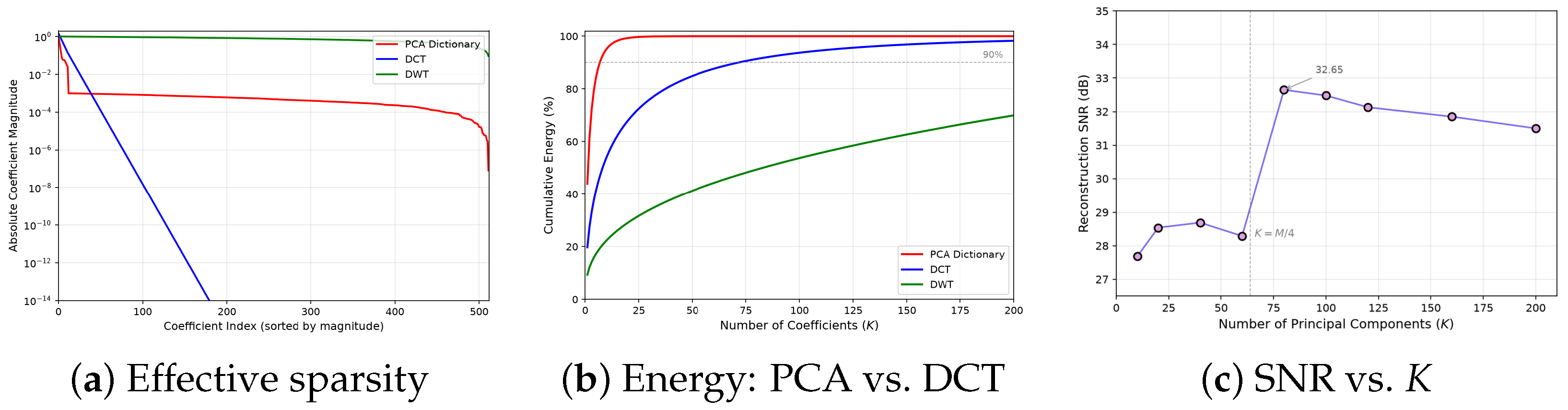
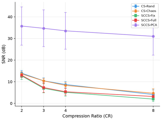
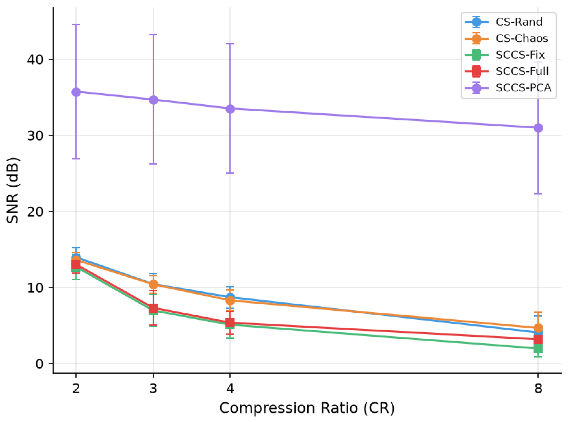
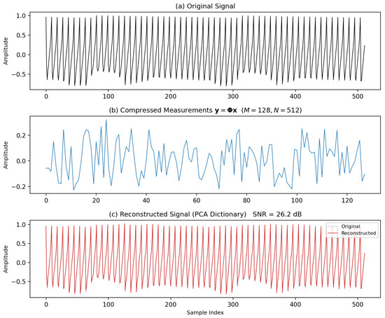
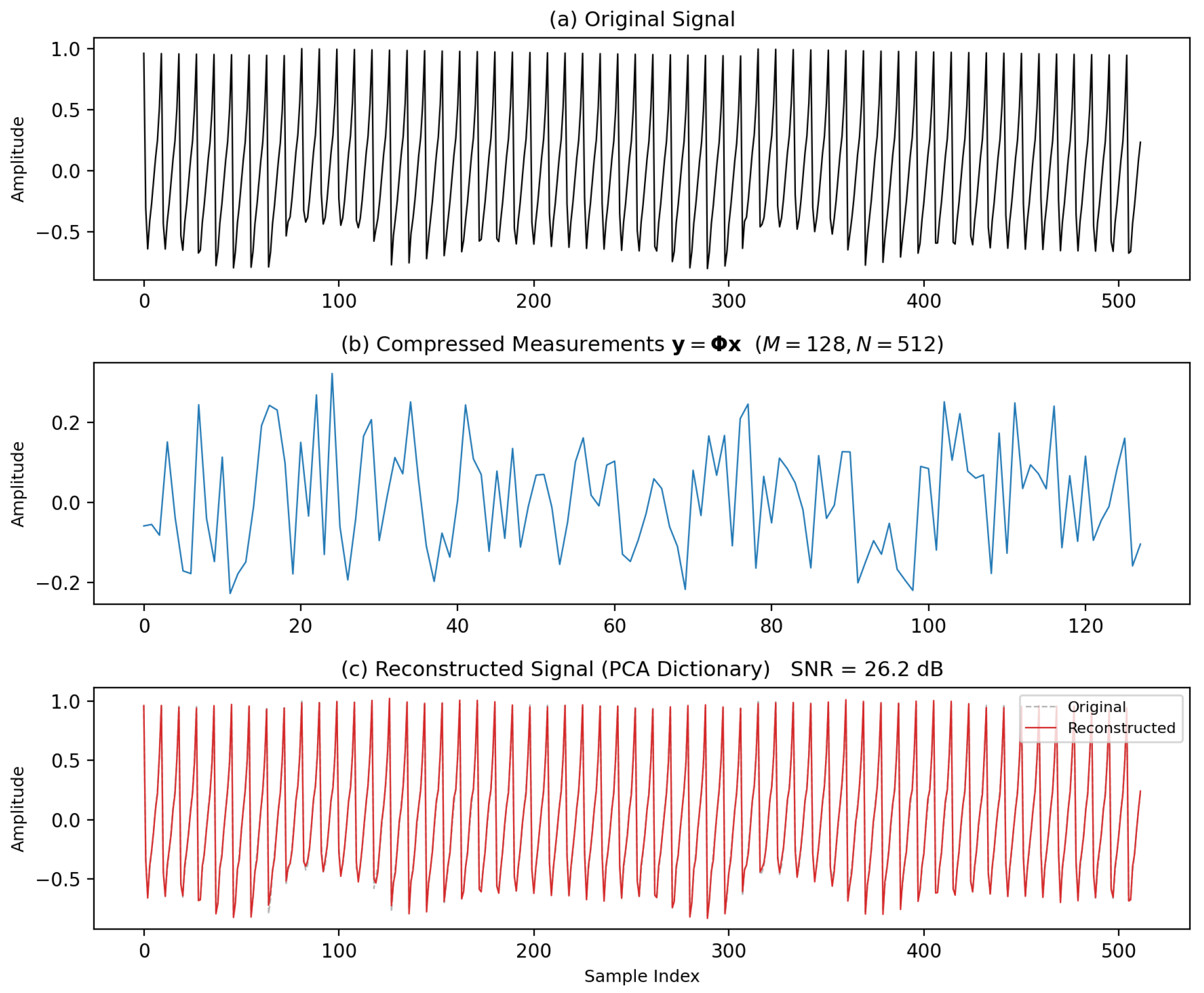
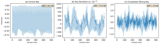
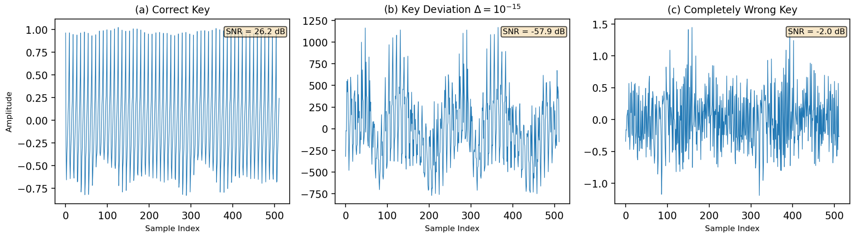
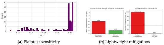
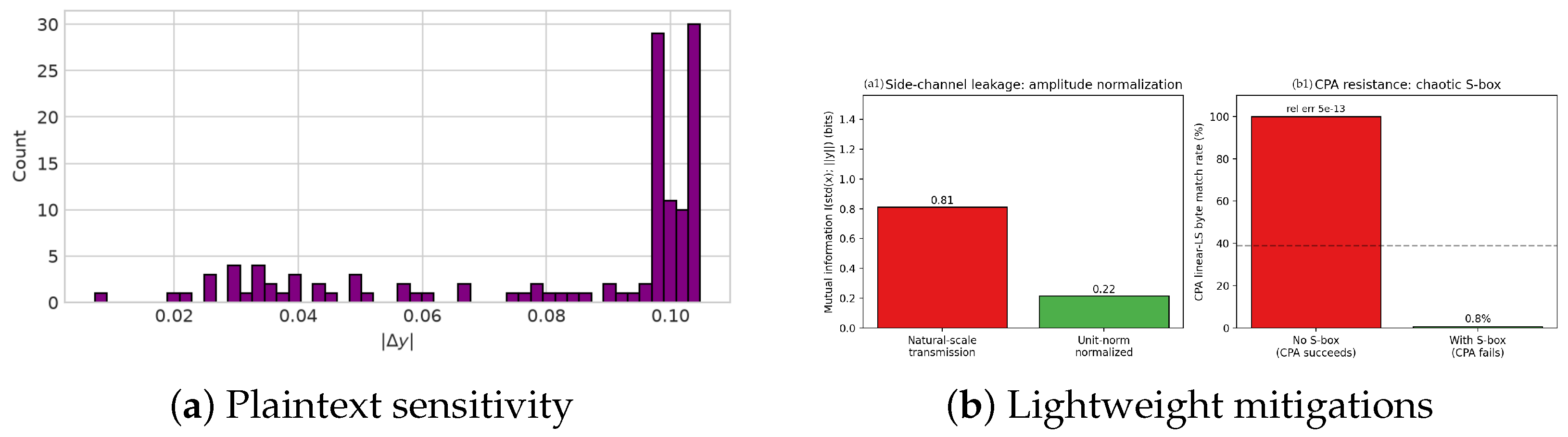
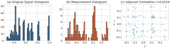
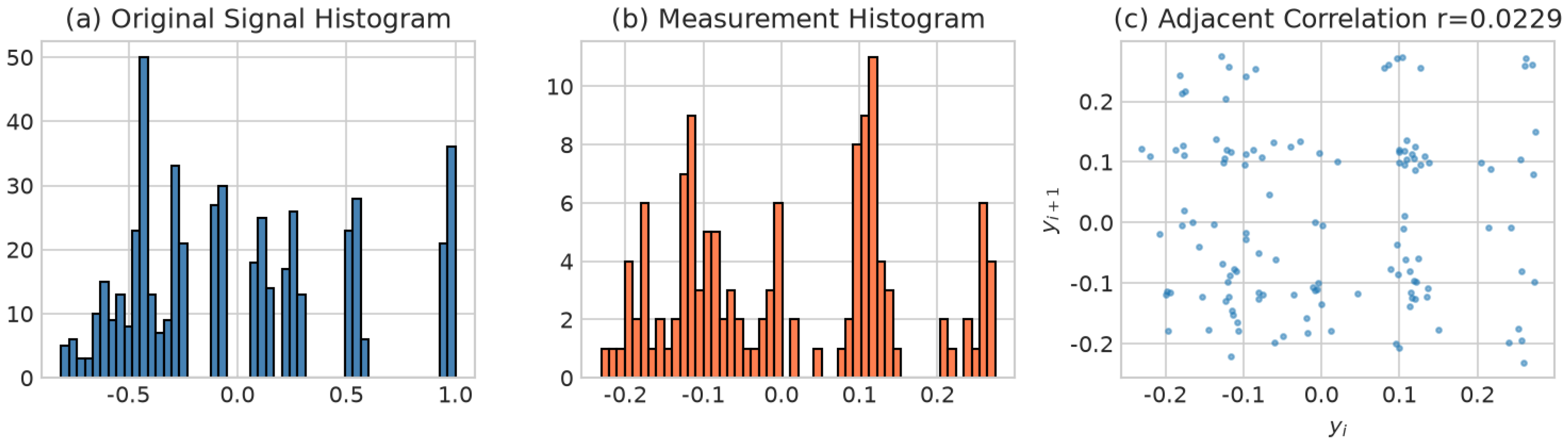
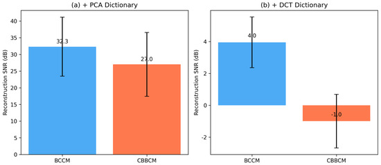
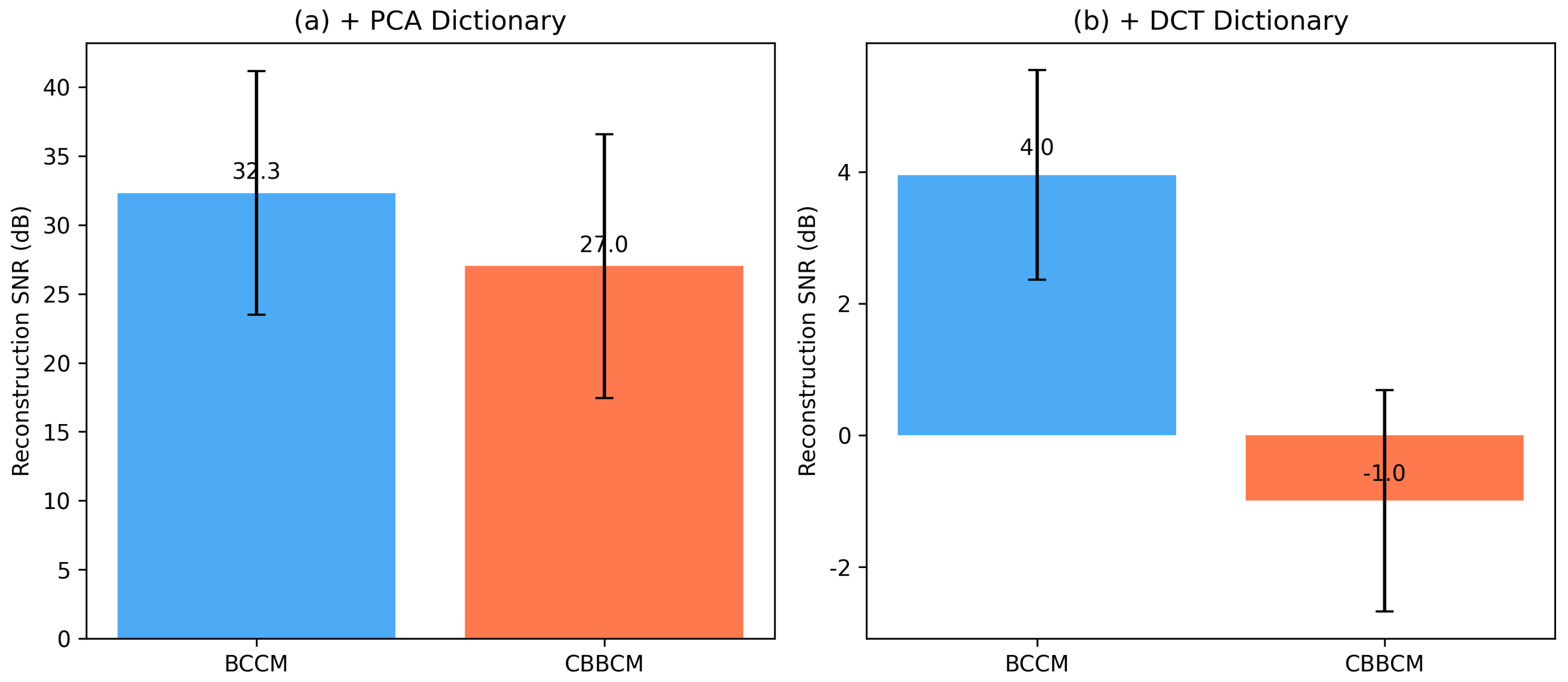
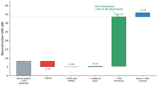
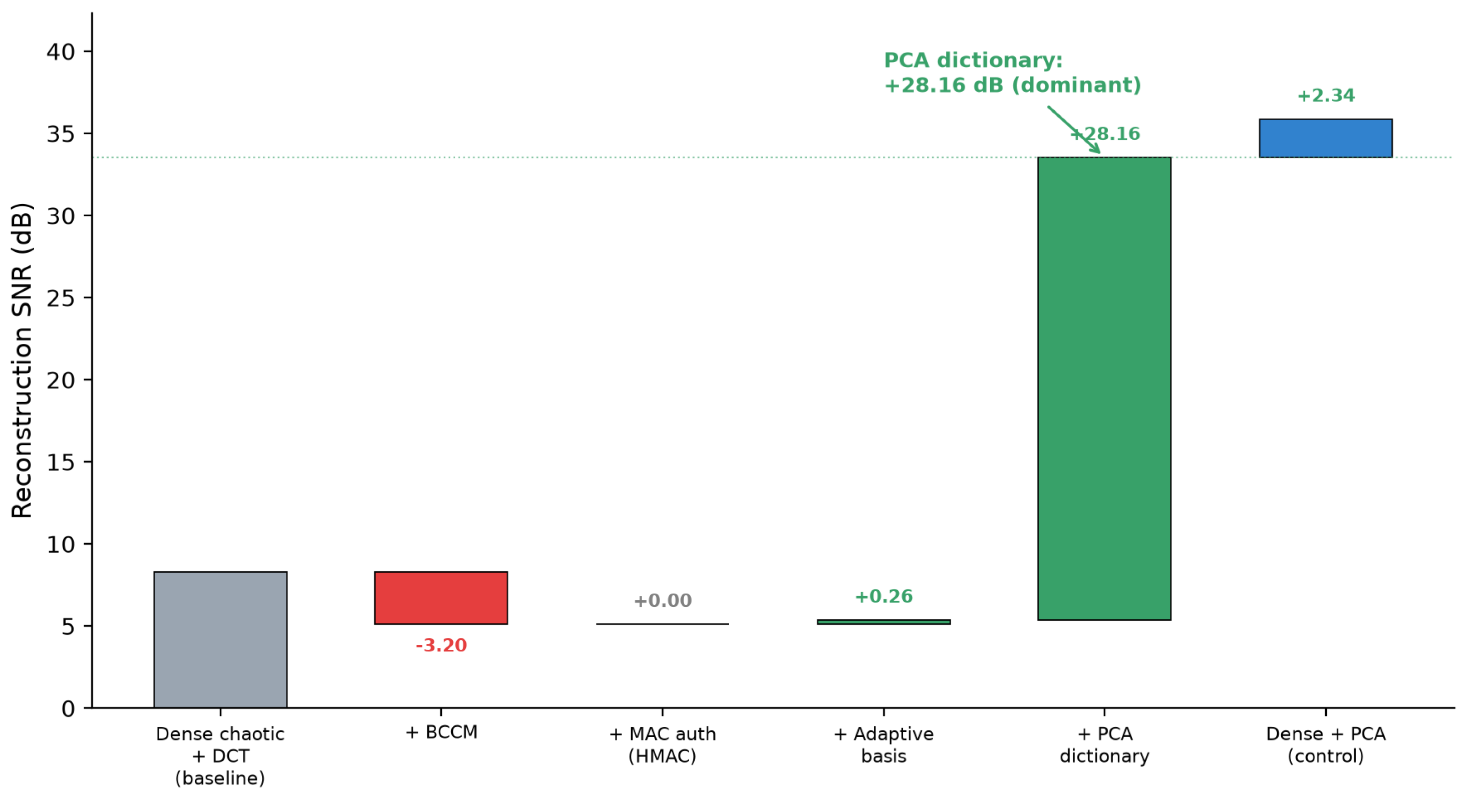
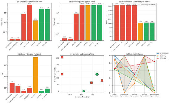
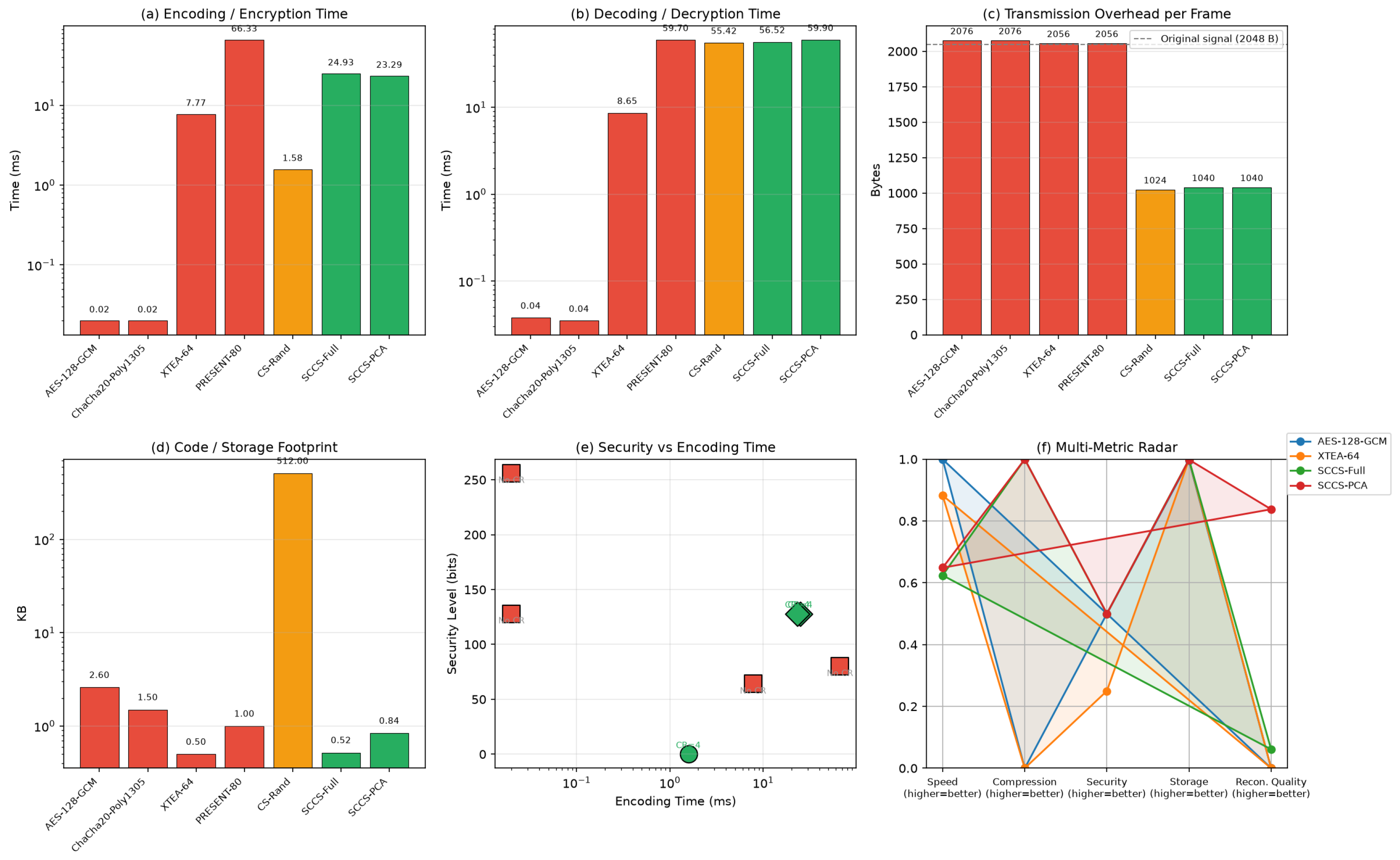
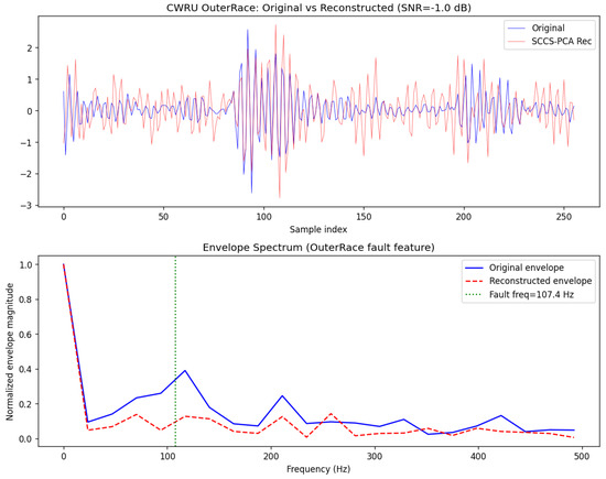
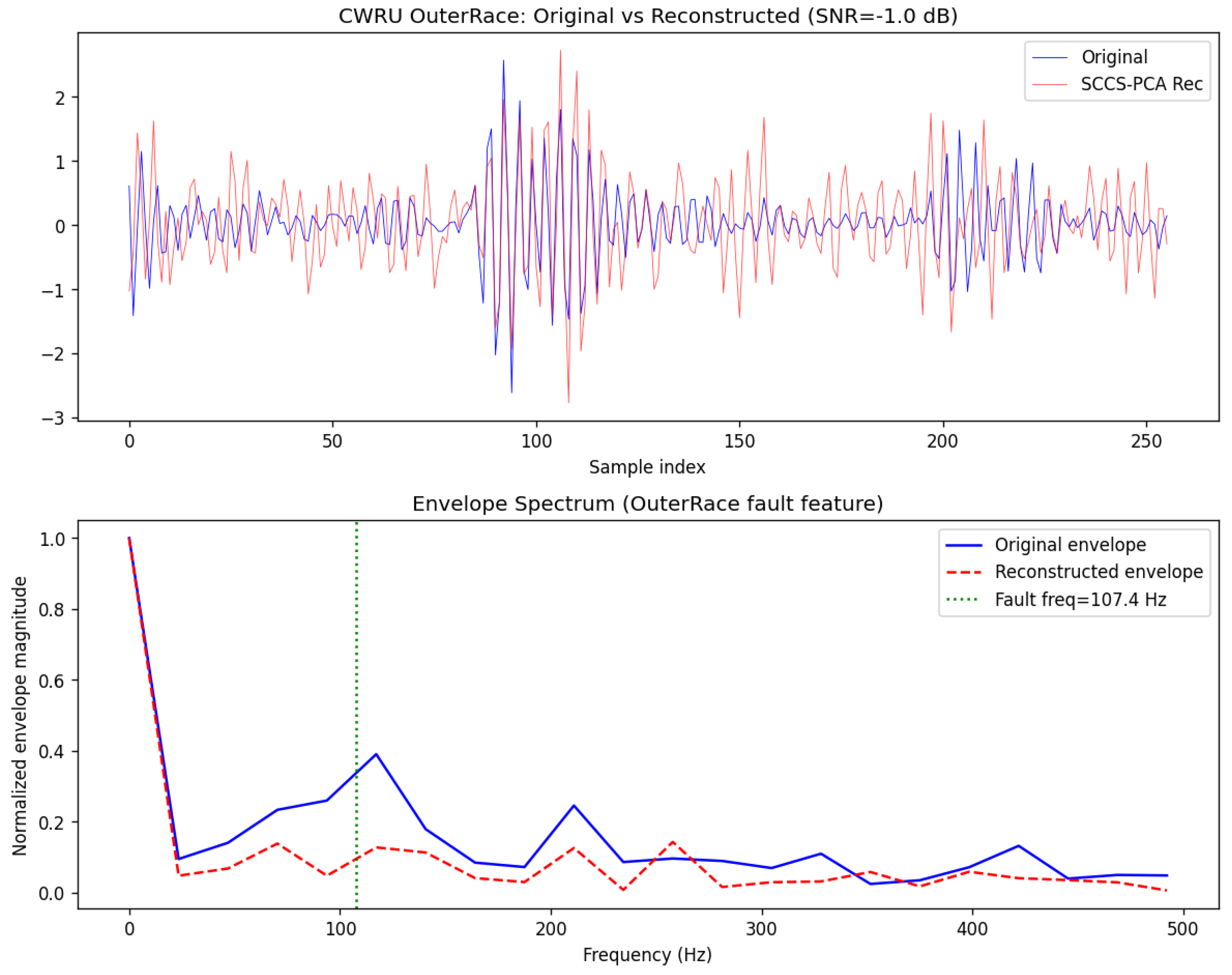
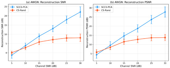
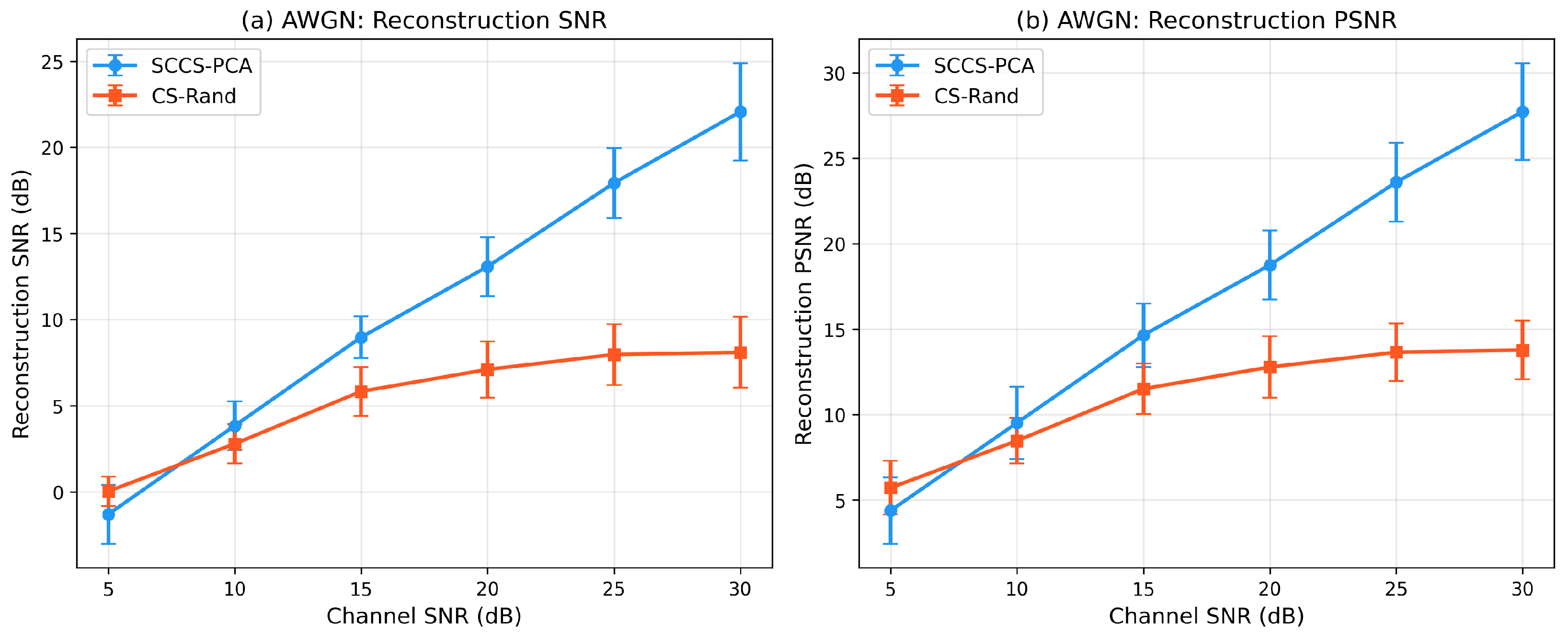
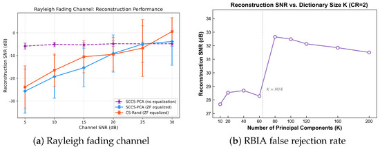
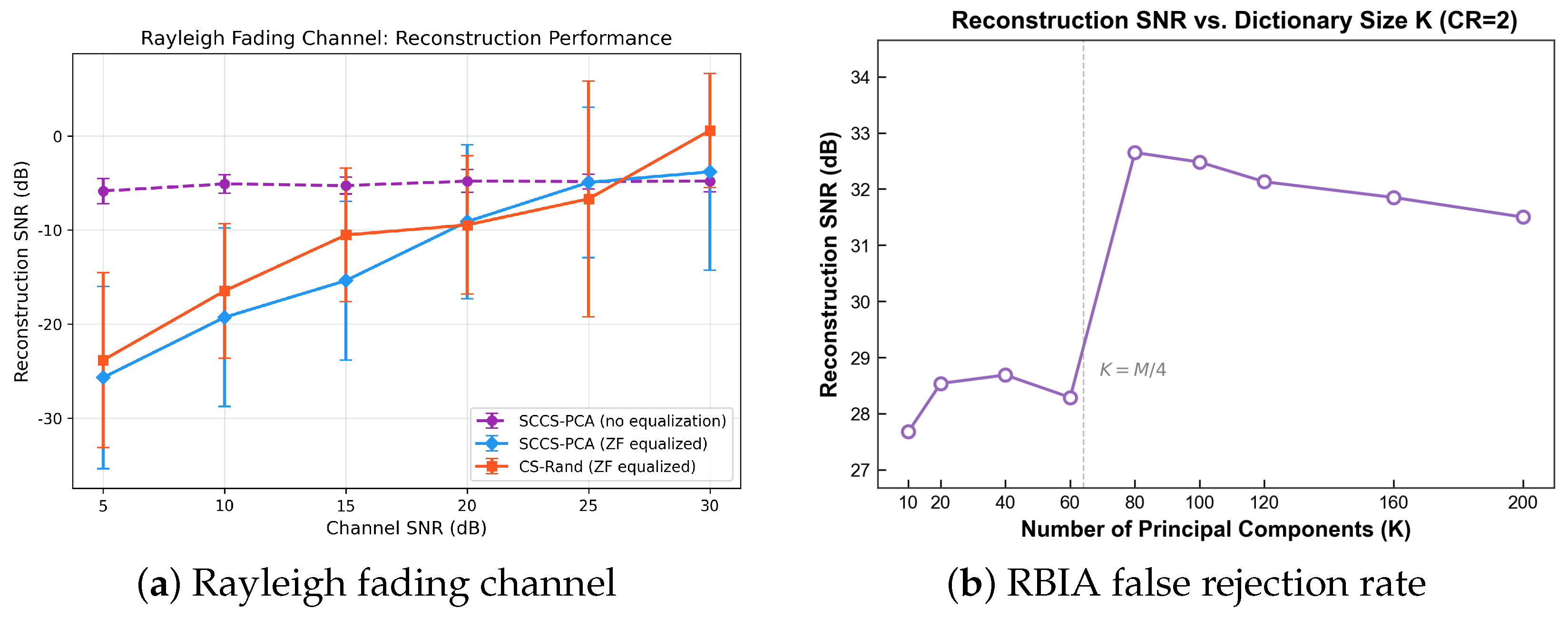
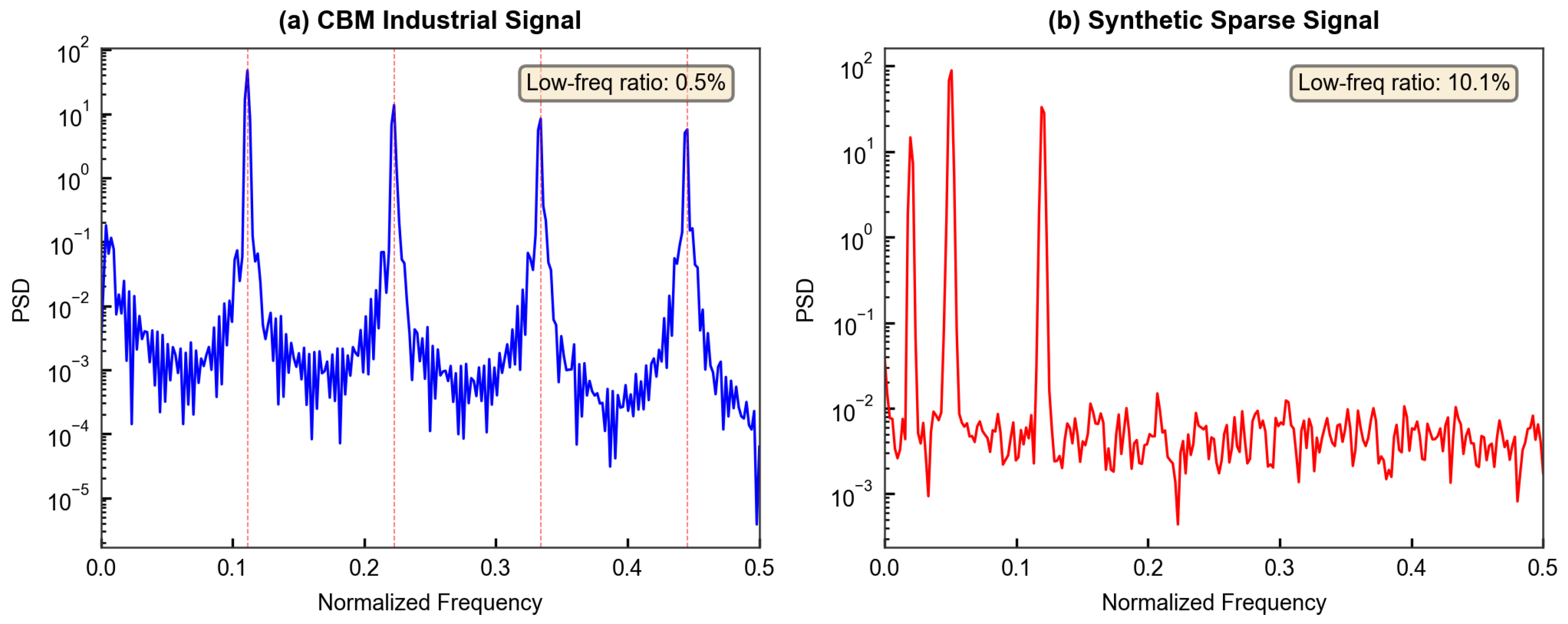

Disclaimer/Publisher’s Note: The statements, opinions and data contained in all publications are solely those of the individual author(s) and contributor(s) and not of MDPI and/or the editor(s). MDPI and/or the editor(s) disclaim responsibility for any injury to people or property resulting from any ideas, methods, instructions or products referred to in the content. |
© 2026 by the authors. Licensee MDPI, Basel, Switzerland. This article is an open access article distributed under the terms and conditions of the Creative Commons Attribution (CC BY) license.