Finite Volume Modeling of Transient Isothermal Hygroscopic Moisture Transport During Solid Wood Processing for Residential Construction

Abstract

Accurate hygrothermal characterization and robust numerical modeling are critical for optimizing timber drying processes and evaluating building envelope performance. This work presents a 1D transient numerical model based on the finite volume method (FVM) and a representative elementary volume (REV) formulation to simulate moisture transport during solid wood drying. The governing nonlinear partial differential equations—incorporating moisture content-dependent diffusivity, liquid suction pressure, and vapor diffusion—were discretized using a fully implicit scheme. The solver was validated against consensus numerical solutions from six international institutions in the HAMSTAD Benchmark No. 2 protocol and further verified against published experimental kinetics. Quantitative error analysis yielded low mean absolute errors (MAE $<0.215 {\mathrm{kg}/\mathrm{m}}^3$) and root mean square errors (RMSE $<0.322 {\mathrm{kg}/\mathrm{m}}^3$) across critical drying stages ($100 \mathrm{h}$, $300 \mathrm{h}$, and $1000 \mathrm{h}$). The proposed framework demonstrates high computational stability and precision, offering a transparent numerical tool for hygrothermal building simulations and timber processing applications.

1. Introduction

Wood is a natural, highly complex material whose properties vary not only between species and individual trees but also within different parts of the same tree [1]. Historically, when woodworking was primarily a traditional craft, these natural variations were deliberately utilized. As a highly heterogeneous and non-uniform material, its structural and behavioral characteristics depend on genetic factors, growth site, post-logging treatment, and service conditions—such as mechanical load, temperature, humidity, and solar radiation. Due to this high variability, wood poses significantly greater challenges in engineering and construction applications compared to synthetic or highly standardized building materials like concrete, steel, and polymer products [2]. Consequently, coupled heat and mass transfer in wood has been extensively studied both experimentally and numerically through various physical models and driving potentials to describe moisture transport.

The definition of driving potentials for moisture transport equations remains a critical area of development [3], as resolving diffusion phenomena through robust numerical schemes provides essential confidence in energy-related simulations. Because analytical solutions are exceptionally difficult to obtain for such nonlinear problems, experimental techniques—despite their inherent uncertainties—remain essential for validating numerical models. A primary challenge lies in accurately capturing coupled heat and mass transfer within porous media. To address this, sophisticated numerical methods must be implemented to solve the governing mathematical models representing these physical phenomena.

In recent years, numerical modeling of heat and moisture transfer in wood has evolved significantly. Modern studies have utilized finite element method (FEM) multiphysics platforms, control volume finite element methods (CVFEMs), and computational fluid dynamics (CFD) to capture local capillary pressures and boundary layer dynamics [4]. However, many existing commercial solvers operate as black-box tools that obscure internal discretization schemes or struggle with nonlinear property jumps at high moisture gradients. State-of-the-art contributions have focused either on highly complex 3D anisotropic multi-scale representations—which require prohibitive computational costs for routine kiln engineering [5]—or on simplified lumped-parameter models that fail to capture local moisture accumulation [6].

To bridge this gap, this study presents a fully transparent, highly robust finite volume method (FVM) framework specifically tailored for transient isothermal hygroscopic moisture transport during solid wood processing. The main innovations of this work are three-fold: (i) an exact implicit nonlinear FVM formulation incorporating moisture-dependent suction pressure gradients without numerical oscillation, (ii) a unified boundary matrix treatment capable of seamlessly switching between strict Dirichlet states and dynamic Robin convective transport without loss of global mass conservation, and (iii) a rigorous, quantitative validation against the benchmark gold-standard HAMSTAD Benchmark No. 2 [7] using statistical error metrics (RMSE and MAE), establishing precise error bounds for isothermal timber drying applications.

2. Methodology

In 2000, the European Union initiated the HAMSTAD (Heat, Air and Moisture STAndards Development) project to establish standardization procedures and certification frameworks in the field of building physics. As a key outcome, five benchmark cases were developed, with multiple consensus numerical solutions subsequently documented by Hagentoft and co-workers in 2004 [7]. In the present work, HAMSTAD Benchmark No. 2 is adopted as the primary validation vehicle because it provides a rigorous basis for comparison with existing solutions and defines a clear acceptance error threshold for numerical codes.

The full title of the HAMSTAD project is “Determination of liquid water transfer properties of porous building materials and development of numerical assessment methods”. The overarching objective of the project was to propose a reference document describing the coupled physics of heat, moisture, and air transfer, including the standard treatment of material properties, boundary conditions, initial conditions, and contact interfaces.

In this study, the computational code is first validated against Benchmark No. 2. Subsequently, the model is applied to evaluate wood samples during the drying process, utilizing the concept of an effective diffusion coefficient alongside experimental data from the literature. Regarding spatial and temporal discretization, interface properties and governing nonlinearities (specifically, source-term linearization) were treated according to the foundational frameworks of Patankar [8] and Maliska [9].

A customized computational code was developed in GNU Octave [10] to solve the coupled system of governing equations, yielding both the transient moisture content profiles and the average moisture content of the domain. Since the stability and accuracy of the finite volume method (FVM) are heavily influenced by the grid density and temporal resolution, a mesh comprising 21 main nodal points and a constant time step of 1 s was selected, following the grid-independence guidelines suggested by Delgado and co-workers [11].

Consequently, the validation stage compares the numerical code outputs with the reference solutions provided by the institutions participating in the HAMSTAD protocol. Finally, the predictive capability of the numerical model is evaluated against the experimental drying results reported by Schellen [12] for beech wood, implementing the average sorption isotherm described in the preceding section.

2.1. Governing Equations and Mathematical Modeling

Within the porous media domain, the governing differential equations for moisture balance are formulated based on the foundational model proposed by Philip and De Vries [13] for moisture diffusion in porous materials. Furthermore, the HAMSTAD protocol framework [14] is implemented using the mathematical approach defined by Dos Santos and Mendes [15] and Mendes and co-workers [16] to establish the specific driving potentials. The transient terms in the governing equations are explicitly expressed as functions of the chosen driving potential, and the resulting linearized system of equations is solved utilizing the tri-diagonal matrix algorithm (TDMA) [17]. Regarding the hygrothermal properties of the material, this work focuses on those highly critical for indoor moisture buffering characterization, specifically the water vapor transmission properties and the moisture sorption isotherm [18].

2.1.1. Porous Media Domain

The mathematical model is formulated based on volume-averaging over a representative elementary volume (REV). This REV is critically defined to be sufficiently large compared to individual pore dimensions to allow meaningful continuum averaging, yet small enough relative to the macroscale macroscopic dimensions of the wood specimen. Under this continuum mechanics framework, the coupled governing equations for heat and moisture transport are established.

2.1.2. Heat and Moisture Transfer

Within the porous media domain, the governing differential equations for moisture balance are formulated based on the foundational model proposed by Philip and De Vries [13] for moisture diffusion in porous materials.

$$c_m{\rho }_0{\displaystyle \frac{\partial T}{\partial t}}=-\nabla q,$$

(1)

$${\displaystyle \frac{\partial w}{\partial t}}=-\nabla g.$$

(2)

Equation (1) describes the energy transport within the porous medium, while Equation (2) represents the moisture transport. Here, $c_m$ denotes the specific heat capacity of the medium [J kg⁻¹ K⁻¹], ${\rho }_0$ is the dry bulk density of the material [kg m⁻³], w represents the moisture content, q is the heat flux, and g is the moisture flux within the porous domain.

2.1.3. Heat

A standard one-dimensional formulation for the coupled heat transfer problem within porous media is expressed as follows:

$$\left(c_{m,\mathrm{dry}}{\rho }_{0,\mathrm{dry}}+c_{l}w\right){\displaystyle \frac{\partial T}{\partial t}}={\displaystyle \frac{\partial }{\partial x}}\left(\lambda \left(\varphi \right){\displaystyle \frac{\partial T}{\partial x}}\right)+L\left({\displaystyle \frac{\partial }{\partial x}}(\delta \left(\varphi \right){\displaystyle \frac{\partial P}{\partial x}}\right).$$

(3)

Here, $c_{m,\mathrm{dry}}$ denotes the specific heat capacity of the dry porous matrix, ${\rho }_{0,\mathrm{dry}}$ is the dry bulk density of the material, $c_l$ is the specific heat capacity of the liquid phase, w represents the moisture content of the medium, $\lambda$ is the effective thermal conductivity of the material, L is the latent heat of vaporization, $\delta$ denotes the water vapor diffusivity, and $\varphi$ is the relative humidity within the porous domain.

2.1.4. Moisture

The moisture transport within the porous medium, as formulated in Equation (2), is defined as follows:

$$-\nabla g=\nabla \left(g_v+g_l\right)=-\left(D_v+{\displaystyle \frac{D_l{R}_{v}T{\rho }_l}{P_v}}\right)\nabla P-D_l{R}_{v}T{\rho }_l\left(Ln\left(\varphi \right)-{\displaystyle \frac{L}{R_{v}T}}\right)\nabla T.$$

(4)

Moisture transport within porous media is driven by two primary mechanisms: vapor diffusion and liquid water flow.

$${\displaystyle \frac{\partial {\rho }_{s}w}{\partial t}}=-\nabla \left(g_v+g_l\right).$$

(5)

Regarding liquid flow, the mathematical formulation is expressed as follows:

$$g_l=k_l{\displaystyle \frac{\partial P_{suc}}{\partial x}}.$$

(6)

Here, $k_l$ represents the liquid water permeability, which is a function of both moisture content and temperature conditions. Conversely, vapor transport comprises both diffusion- and convection-driven components.

$$g_v=-{\delta }_v{\displaystyle \frac{\partial p}{\partial x}}+r_a{v}_a.$$

(7)

Regarding the diffusive transport component, ${\delta }_v$ denotes the vapor permeability, which is a function of the moisture content. In the convective transport component, $v_a$ represents the water vapor concentration, defined as the absolute humidity expressed per unit volume.

2.1.5. Sorption Processes in Wood for Building Physics

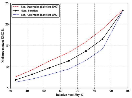
For certain building materials, the discrepancy between the adsorption and desorption isotherms is negligible, meaning a single isotherm suffices to characterize the equilibrium moisture state. However, this simplified assumption does not hold for wood due to its pronounced hysteretic behavior. While the practical necessity of explicitly modeling hysteresis in building physics remains a subject of ongoing discussion, an average isotherm between the adsorption and desorption curves is frequently adopted for engineering applications, as suggested by Woodruff and Revil [19]. This averaged approach is implemented in the present work. Figure 1 illustrates the equilibrium moisture content data obtained by Schellen [12] for a beech wood specimen. In this figure, the lower blue dotted line represents the adsorption boundary curve, the upper red dotted line represents the desorption boundary curve, and the solid black line corresponds to the average isotherm implemented in the numerical model.

Figure 1. Sorption isotherm for beech wood.

2.1.6. Model Assumptions and Scope of Application

To establish a mathematically controlled baseline for verifying the numerical accuracy, spatial/temporal stability, and algorithmic convergence of the proposed finite volume method (FVM) solver, the model formulation strictly adheres to the standardized protocol of the HAMSTAD Benchmark No. 2 (EU Project SMT4-CT97-2194) [7]. This benchmark isolates 1D transient vapor diffusion from secondary multiphysical coupling (such as thermal gradients, liquid capillary advection, and phase-change enthalpy) to evaluate spatial discretization precision independently of experimental or physical noise.

Based on this international benchmark specification, the mathematical model relies on the following seven fundamental assumptions:

(1)

Isothermal conditions ($T=\mathrm{const}.$) are assumed throughout the wood domain.

(2)

One-dimensional (1D) transient moisture diffusion across the thickness of the wood specimen.

(3)

Moisture transport is governed exclusively by vapor pressure gradients within the hygroscopic range ($\varphi <95\%$, below the fiber saturation point).

(4)

Local thermodynamic equilibrium between the pore air space and the surrounding cell wall matrix.

(5)

Rigid and isotropic porous matrix with constant mechanical dimensions (swelling and shrinkage effects are neglected).

(6)

Single-phase mass transport without liquid water capillary flow.

(7)

Negligible hysteresis between the absorption and desorption equilibrium curves for the benchmark evaluation.

Solid wood is inherently orthotropic, exhibiting significantly higher diffusion along the longitudinal grain than in transverse (radial and tangential) directions. However, in wide structural timber planks, transient moisture transport is overwhelmingly dominated by flux across the principal minimum thickness dimension ($L_x=0.2\mathrm{m}$). Due to high geometric aspect ratios ($L_y/L_x\gg 5$ and $L_z/L_x\gg 10$), boundary edge fluxes contribute negligibly to the overall mass balance. Therefore, modeling moisture movement along a single spatial axis (x) using effective transverse transport properties provides an accurate representation of macroscale hygroscopic kinetics. By adhering to these validated benchmark constraints, the proposed 1D FVM framework is specifically suitable for predicting transient moisture distribution in engineered solid wood elements operating under quasi-isothermal conditions in building envelopes, providing a computationally efficient tool for engineering design prior to executing fully coupled multiphysics simulations.

2.2. Numerical Method

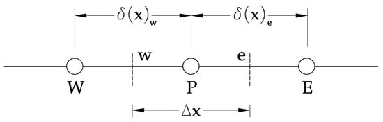
The finite volume method (FVM), implemented in a transient, fully implicit, and one-dimensional configuration, was adopted to discretize the governing equations. The spatial domain is divided into discrete control volumes, where the integration of the governing conservation laws over each control volume ($\Delta x$) and temporal step ($\Delta t$) ensures the rigorous balance of heat and mass quantities across the system boundaries. Figure 2 illustrates the schematic representation of the mesh and a typical control volume layout.

Figure 2. Finite volume method discretization.

Following the discretization framework described by Tariku and co-workers [20], the resulting algebraic equations can be expressed as:

$${\int }_t^{t+\Delta t}{\int }_w^e\psi {\displaystyle \frac{\partial P_v}{\partial t}}dxdt={\int }_t^{t+\Delta t}{\int }_w^e\xi {\displaystyle \frac{\partial P_v}{\partial x}}dxdt,$$

(8)

$$\psi ={\displaystyle \frac{\partial w}{\partial \varphi }}{\displaystyle \frac{1}{P_{sat}}},$$

(9)

$$\xi =D_v+{\displaystyle \frac{D_l{R}_{v}T{\rho }_l}{P_v}}.$$

(10)

To close the mathematical model, the following constitutive and auxiliary relations are required to determine the moisture- and temperature-dependent material properties:

$$P_{sat}=0.618\times e^{{\displaystyle \frac{17.269T}{T+273.3}}},$$

(11)

$${\displaystyle \frac{\partial w}{\partial \varphi }}={\displaystyle \frac{854.271}{\varphi {(1-8.47458ln\left(\varphi \right))}^{1.869}}},$$

(12)

$$\varphi ={\displaystyle \frac{P_v}{P_{sat}}}.$$

(13)

2.3. Internal Control Volumes

The governing 1D transient moisture diffusion equation is discretized over control volume $\Delta x$ and time step $\Delta t$. For an internal node P, the integrated mass balance is:

$$\left({\displaystyle \frac{\partial w}{\partial \varphi }}{\displaystyle \frac{1}{P_{\mathrm{sat}}}}\right)\left({\displaystyle \frac{P_P-P_P^0}{\Delta t}}\right)\Delta x={\displaystyle \frac{\xi }{\Delta x}}(P_E-P_P)-{\displaystyle \frac{\xi }{\Delta x}}(P_P-P_W).$$

(14)

Expanding Equation (14) yields:

$$A_P{P}_P-A_P^0{P}_P^0=A_E{P}_E-A_E{P}_P-A_W{P}_P+A_W{P}_W.$$

(15)

Grouping the central node variable $P_P$ on the left-hand side leads to the canonical TDMA matrix system in

$$\left(A_P\right)P_P=A_E{P}_E+A_W{P}_W+A_P^0{P}_P^0,$$

(16)

where the algebraic coefficients are defined as:

$$\begin{array}{cc}\hfill A_E& ={\displaystyle \frac{\xi }{\Delta x}}[\mathrm{Eastern} \mathrm{neighbor} \mathrm{conductance} \mathrm{coefficient}];\hfill \end{array}$$

(17)

$$\begin{array}{cc}\hfill A_W& ={\displaystyle \frac{\xi }{\Delta x}}[\mathrm{Western} \mathrm{neighbor} \mathrm{conductance} \mathrm{coefficient}];\hfill \end{array}$$

(18)

$$\begin{array}{cc}\hfill A_P^0& =\left({\displaystyle \frac{\partial w}{\partial \varphi }}{\displaystyle \frac{1}{P_{\mathrm{sat}}}}\right){\displaystyle \frac{\Delta x}{\Delta t}}[\mathrm{Transient} \mathrm{storage} \mathrm{coefficient} \mathrm{at} \mathrm{previous} \mathrm{time} \mathrm{step} t];\hfill \end{array}$$

(19)

$$\begin{array}{cc}\hfill A_P& =A_E+A_W+A_P^0[\mathrm{Central} \mathrm{node} \mathrm{main} \mathrm{diagonal} \mathrm{coefficient}].\hfill \end{array}$$

(20)

In the above, $\xi =D_v+{\displaystyle \frac{D_l{R}_{v}T{\rho }_l}{P_v}}$ is the effective moisture transport property, $\Delta t$ [s] is the time step, $\Delta x$ [m] is the spatial mesh size, $P_P^0$ is the vapor pressure at t, and $P_P,P_E,P_W$ are the unknown vapor pressures at $t+\Delta t$.

2.4. Left Boundary Control Volume (Dirichlet)

For the control volume at the left boundary ($x=0$), the distance from node P to the exterior boundary surface ($P_{\mathrm{ext}}$) is $\Delta x/2$. The discretized balance equation is:

$$\left({\displaystyle \frac{\partial w}{\partial \varphi }}{\displaystyle \frac{1}{P_{\mathrm{sat}}}}\right)\left({\displaystyle \frac{P_P-P_P^0}{\Delta t}}\right)\Delta x={\displaystyle \frac{\xi }{\Delta x}}(P_E-P_P)-2{\displaystyle \frac{\xi }{\Delta x}}(P_P-P_{\mathrm{ext}}).$$

(21)

Expanding the algebraic terms yields:

$$A_P{P}_P-A_P^0{P}_P^0=A_E{P}_E-A_E{P}_P-2A_W{P}_P+2A_W{P}_{\mathrm{ext}}.$$

(22)

Rearranging into the standard TDMA matrix form gives:

$$(A_E+2A_W+A_P^0)P_P=A_E{P}_E+2A_W{P}_{\mathrm{ext}}+A_P^0{P}_P^0,$$

(23)

where $2A_W={\displaystyle \frac{2\xi }{\Delta x}}$ accounts for the half-cell distance to the left boundary surface.

2.5. Right Boundary Control Volume (Dirichlet)

Similarly, for the control volume at the right boundary ($x=L$), subject to internal prescribed boundary value $P_{\mathrm{int}}$, the balance equation is:

$$\left({\displaystyle \frac{\partial w}{\partial \varphi }}{\displaystyle \frac{1}{P_{\mathrm{sat}}}}\right)\left({\displaystyle \frac{P_P-P_P^0}{\Delta t}}\right)\Delta x=2{\displaystyle \frac{\xi }{\Delta x}}(P_{\mathrm{int}}-P_P)-{\displaystyle \frac{\xi }{\Delta x}}(P_P-P_W).$$

(24)

Expanding yields:

$$A_P{P}_P-A_P^0{P}_P^0=2A_E{P}_{\mathrm{int}}-2A_E{P}_P-A_W{P}_P+A_W{P}_W.$$

(25)

Rearranging into the TDMA standard form gives:

$$(A_W+2A_E+A_P^0)P_P=A_W{P}_W+2A_E{P}_{\mathrm{int}}+A_P^0{P}_P^0,$$

(26)

where $2A_E={\displaystyle \frac{2\xi }{\Delta x}}$ accounts for the half-cell distance to the right boundary surface.

2.6. Left and Right Boundary Control Volume (Robin)

Regarding the boundary control volume adjacent to the left surface under Robin boundary conditions, the convective heat and mass fluxes alter the balance equation, yielding the following discretized form:

$$j_{ext}={\beta }_{p,e}(P_{v,ext}-P_{v,sup}),$$

(27)

$${\displaystyle \frac{\partial w}{\partial \varphi }}{\displaystyle \frac{1}{P_{sat}}}\left({\displaystyle \frac{P_P-P_P^0}{2\Delta t}}\right)\Delta x={\displaystyle \frac{\xi }{\Delta x}}(P_E-P_P)-j_{ext}.$$

(28)

Similarly, for the boundary control volume adjacent to the right surface under Robin boundary conditions, the convective environmental exchanges are integrated into the balance, leading to the following discretized expression:

$$j_{int}={\beta }_{p,i}(P_{v,int}-P_{v,sup}),$$

(29)

$${\displaystyle \frac{\partial w}{\partial \varphi }}{\displaystyle \frac{1}{P_{sat}}}\left({\displaystyle \frac{P_P-P_P^0}{2\Delta t}}\right)\Delta x=j_{int}-{\displaystyle \frac{\xi }{\Delta x}}(P_P-P_W).$$

(30)

3. Benchmark Validation and Computational Setup

To validate the proposed numerical framework, a computational code was developed based on the HAMSTAD Benchmark No. 2 protocol. This baseline involves the spatial and temporal discretization of the governing partial differential equations via the finite volume method (FVM), alongside the rigorous formulation of their respective boundary conditions. The core physical problem and its specifications are described in detail below. Furthermore, the predictive accuracy of the numerical code was validated against the experimental results presented by Schellen [12], as detailed in Section 3.2.

3.1. HAMSTAD Benchmark No. 2

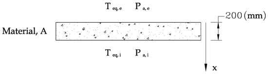
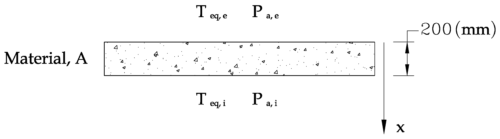
This second benchmark case addresses transient moisture redistribution within a single material layer under isothermal conditions. The moisture transport is driven by a step change in the relative humidity of the surrounding environment. A homogeneous, one-dimensional porous layer is analyzed. Initially, the material is in hygroscopic equilibrium with the ambient air at a constant relative humidity. At $t=0$, a sudden asymmetric change occurs in the relative humidity of the surrounding air. The structure is assumed to be completely airtight, neglecting any convective bulk air flow through the material. Figure 3 illustrates the schematic representation of the test specimen, delineating the internal and external boundary conditions.

Figure 3. Structure geometry.

3.1.1. Properties of Material

The hygrothermal properties and benchmark parameters evaluated in the HAMSTAD Benchmark No. 2 protocol are explicitly defined as follows:

• Sorption Isotherm $w\left(\varphi \right)$: Relates volumetric moisture content w to relative humidity $\varphi$:

  $$w\left(\varphi \right)=116{\left[1-{\displaystyle \frac{1}{0.118}}ln\varphi \right]}^{-0.869}[\mathrm{kg}·{\mathrm{m}}^{-3}].$$

  (31)
• Vapor Permeability ${\delta }_P$: Constant vapor transport coefficient:

  $${\delta }_P=1.0\times {10}^{-15}\left[\mathrm{s}\right].$$

  (32)
• Moisture Diffusivity $D_w\left(w\right)$: Nonlinear moisture transport property combining liquid suction and vapor movement:

  $$D_w\left(w\right)=-K{\displaystyle \frac{\partial P_{\mathrm{suc}}}{\partial w}}+{\displaystyle \frac{{\delta }_P{P}_s}{\xi }}[{\mathrm{m}}^2·{\mathrm{s}}^{-1}],$$

  (33)

  where K is hydraulic permeability, $P_s$ is saturation vapor pressure, and $\xi =\mathrm{d}w/\mathrm{d}\varphi$ is moisture capacity. The derivative of suction pressure with respect to moisture content ${\displaystyle \frac{\partial P_{\mathrm{suc}}}{\partial w}}$ is expressed as:

  $${\displaystyle \frac{\partial P_{\mathrm{suc}}}{\partial w}}=-{\displaystyle \frac{RT{\rho }_w}{M_w\varphi \xi }}[\mathrm{Pa}·{\mathrm{m}}^3·{\mathrm{kg}}^{-1}].$$

  (34)
• Thermal Conductivity $\lambda$: Constant effective value:

  $$\lambda =0.15[\mathrm{W}·{\mathrm{m}}^{-1}·{\mathrm{K}}^{-1}].$$

  (35)
• Specific Heat Capacity $c_p$: Dry state value:

  $$c_p=800[\mathrm{J}·{\mathrm{kg}}^{-1}·{\mathrm{K}}^{-1}].$$

  (36)
• Dry Bulk Density ${\rho }_0$: Reference solid density:

  $${\rho }_0=525[\mathrm{kg}·{\mathrm{m}}^{-3}].$$

  (37)
• Geometrical Thickness $L_x$: Principal spatial dimension along coordinate x:

  $$L_x=0.20\left[\mathrm{m}\right].$$

  (38)

3.1.2. Boundary and Initial Conditions

The simulation parameters, including environmental loads, surface transfer coefficients, and initial states, are systematically defined below. The equivalent environmental temperatures, which encompass both ambient air temperatures and radiative heat exchange, are kept constant:

$$\begin{array}{c}\hfill T_{\mathrm{eq},e}=20 °\mathrm{C},T_{\mathrm{eq},i}=20 °\mathrm{C}.\end{array}$$

At $t=0$, an instantaneous step change in the ambient relative humidity is imposed, leading to asymmetric boundary profiles described by:

$$\begin{array}{cc}\hfill {\varphi }_{a,e}\left(t\right)& =0.45(\mathrm{exterior} \mathrm{boundary});\hfill \\ \hfill ph{i}_{a,i}\left(t\right)& =0.65(\mathrm{interior} \mathrm{boundary}).\hfill \end{array}$$

The convective heat ($\alpha$) and vapor (${\beta }_p$) surface transfer coefficients are defined symmetrically for both faces as follows:

$$\begin{array}{cc}\hfill {\alpha }_{e,e}& =25{\displaystyle \frac{\mathrm{W}}{{\mathrm{m}}^2·\mathrm{K}}},{\alpha }_{e,i}=25{\displaystyle \frac{\mathrm{W}}{{\mathrm{m}}^2·\mathrm{K}}}.\hfill \\ \hfill {\beta }_{p,e}& =1.0\times {10}^{-3}{\displaystyle \frac{\mathrm{s}}{\mathrm{m}}},{\beta }_{p,i}=1.0\times {10}^{-3}{\displaystyle \frac{\mathrm{s}}{\mathrm{m}}}.\hfill \end{array}$$

The spatial domain is initialized under uniform hygroscopic and thermal equilibrium conditions:

$$\begin{array}{c}\hfill \varphi (x,0)=95.\end{array}$$

3.1.3. Numerical Output Requirements

The computational implementation complies with the following protocol specifications:

(i)

Total simulation period: 1000 h.

(ii)

Requested profiles: The cross-sectional distribution of the material moisture content (w) must be evaluated and reported at transient intervals of 100 h, 300 h, and 1000 h.

3.2. Experimental Data

As previously indicated, the reference experimental datasets for the validation study were obtained from the literature, specifically from the comprehensive work on the drying behavior of historical building components detailed by Schellen [12]. In that study, transient moisture transport within porous wood specimens under varying climatic conditions was monitored using advanced nuclear magnetic resonance (NMR) scanners developed at the Center for Material Research with Magnetic Resonance at the Eindhoven University of Technology—a high-fidelity non-destructive measurement methodology documented extensively by Johnson [21] and Roels and co-workers [18].

The NMR experimental configuration consists of a cylindrical radiofrequency (RF) coil positioned within a homogeneous magnetic field, where the material samples are inserted. This specialized scanner enables the quantitative evaluation of moisture profiles with a spatial resolution of 0.5 mm. To subject the specimen to dynamically controlled thermal and hygrometric conditions, a wooden cylinder measuring 25 mm in diameter and 200 mm in length is centered inside an outer Perspex flow tube with an inner diameter of 50 mm and a total length of 1500 mm. The conditioned airstream is generated by blending dry and saturated air masses, which is subsequently introduced into the chamber to establish a well-defined axial airflow along the exposed surface of the wooden sample. To guarantee a hydrodynamically developed, laminar boundary layer and prevent leading-edge flow separation, a synthetic dummy specimen with an aerodynamic pointed profile is positioned directly upstream of the wood sample. The temperature and relative humidity of the air are continuously monitored at both the inlet and outlet boundaries of the Perspex assembly.

The experimental validation campaigns were conducted strictly within the hygroscopic regime of the material. To fully characterize the hygroscopic performance of the wood, key transport and storage material properties were experimentally determined, namely the vapor diffusion resistance factor and the moisture sorption isotherm, which together govern the dynamic equilibrium between the internal moisture content and the boundary microclimate.

The vapor diffusion resistance measurements were carried out in a climatic chamber under strictly isothermal conditions at 20 °C across two distinct relative humidity gradients: from 85% down to 33% RH (yielding a mean value of 59% RH) and from 85% down to 53% RH (yielding a mean value of 69% RH). The resulting experimental transport properties are summarized in Table 1.

Table 1. Vapor diffusion of beech wood.

Mean Relative Humidity RH %	Thickness d (mm)	Mean Vapor Diffusion Resistance $\mathit{\mu }$ (-)
59	10.0	27 ± 2
59	15.0	37 ± 2
69	10.0	35 ± 1
69	15.0	67 ± 13

• Moisture Diffusivity: The transient moisture profiles acquired via NMR were utilized to determine the effective moisture diffusivity ($D_w$) of the wood by solving the inverse mass transport problem. The experimental profiles recorded during the drying phase served as the target benchmark. An optimization-based numerical fitting procedure was deployed to minimize the residuals between the measured and simulated moisture distributions, yielding a calibrated effective moisture diffusivity of $D_w=5.9\times {10}^{-10}{\mathrm{m}}^2/\mathrm{s}$.
• Boundary Conditions: Although the convective surface vapor transfer coefficients were not explicitly characterized in the original experimental campaign, the authors utilized them primarily as adjustable parameters for mathematical fitting. To eliminate the uncertainty associated with estimating film coefficients (${\beta }_p$) and to isolate the internal transport mechanisms, the validation code developed in this study was implemented by prescribing time-dependent Dirichlet boundary conditions derived directly from the experimental surface moisture data.

4. Results and Discussion

This section presents the results for the first validation using data available from the HAMSTAD protocol. Following this, the validation of the numerical code against experimental data for a drying solid wood specimen will be shown.

4.1. Results for the First Validation

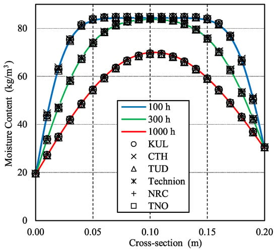
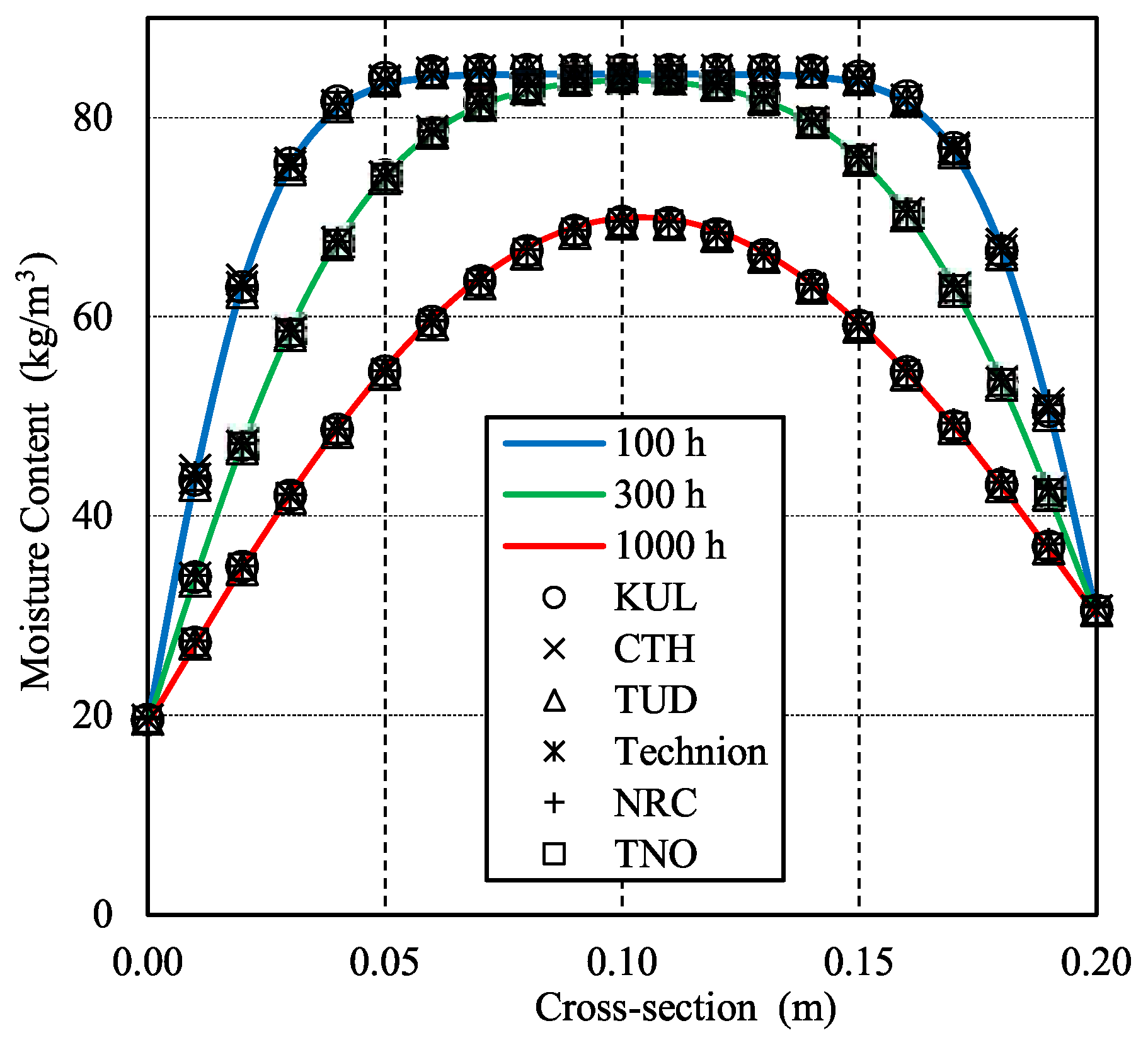
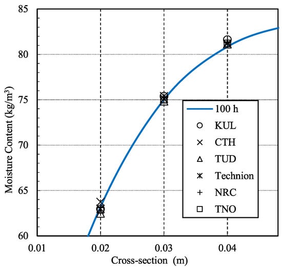
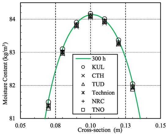
In this section, the primary data are presented graphically to compare our findings with key participants in the HAMSTAD protocol—including Chalmers University of Technology (CTH), K.U. Leuven, Belgium (KUL), the National Research Council of Canada (NRC), The Technion–Israel Institute of Technology (Technion), TNO Building and Construction Research (TNO), and the Technical University of Dresden (TUD)—as presented in Hagentoft [14]. Figure 4 displays the results for the 100, 300, and 1000 h simulations required by the protocol. The continuous lines represent the simulation results, while the discrete symbols show the results of each participant in the HAMSTAD protocol. In general, a good correlation between the datasets is observed, demonstrating that the objective of modeling the diffusion process in a homogeneous material has been successfully achieved.

Figure 4. Numerical solution for moisture content within the HAMSTAD benchmark.

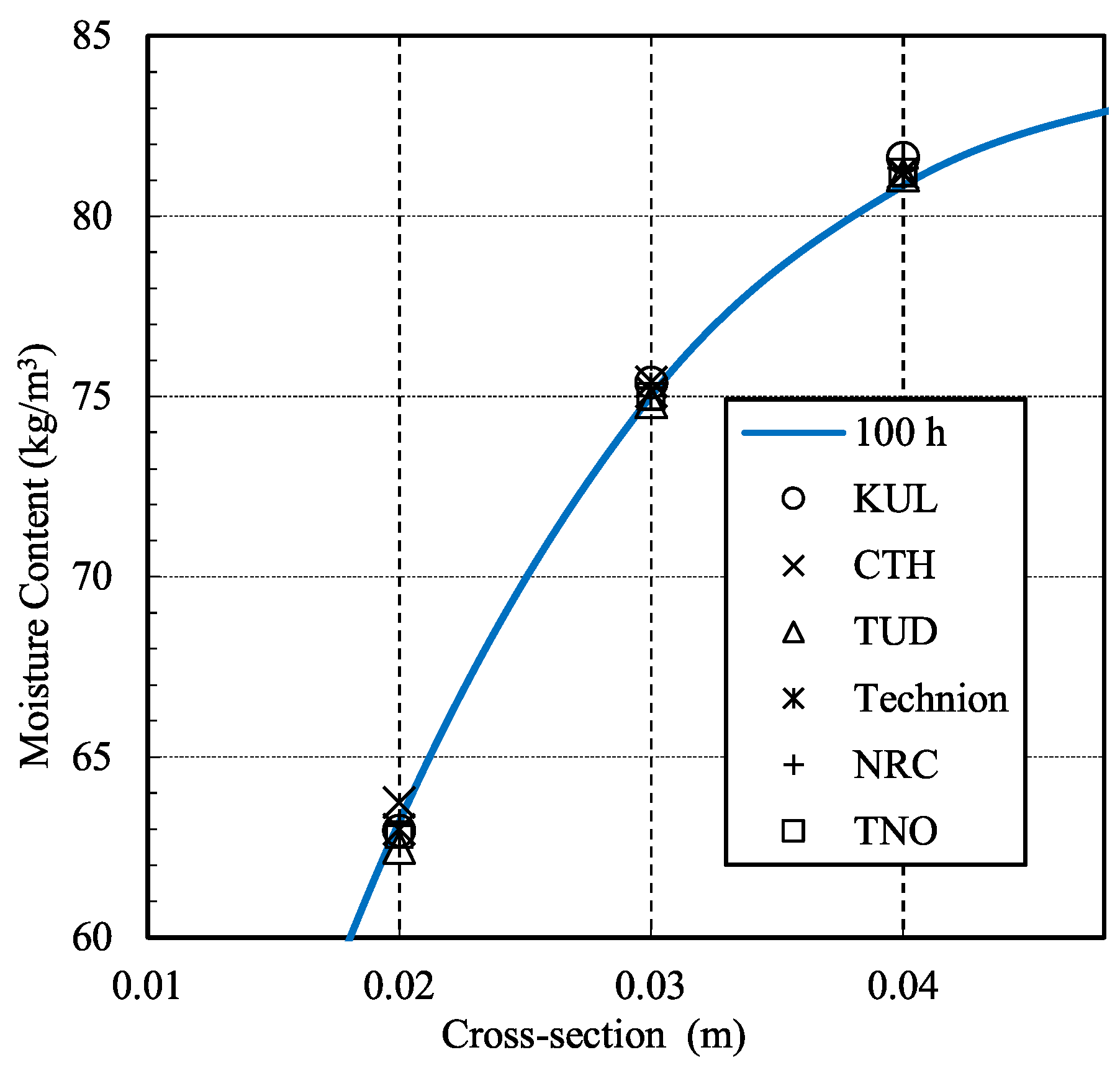
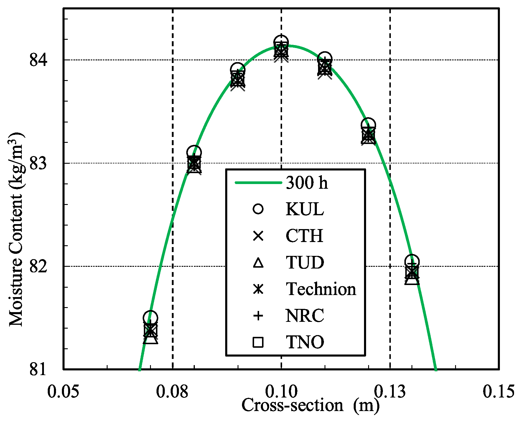
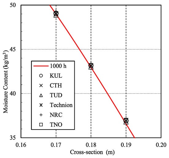
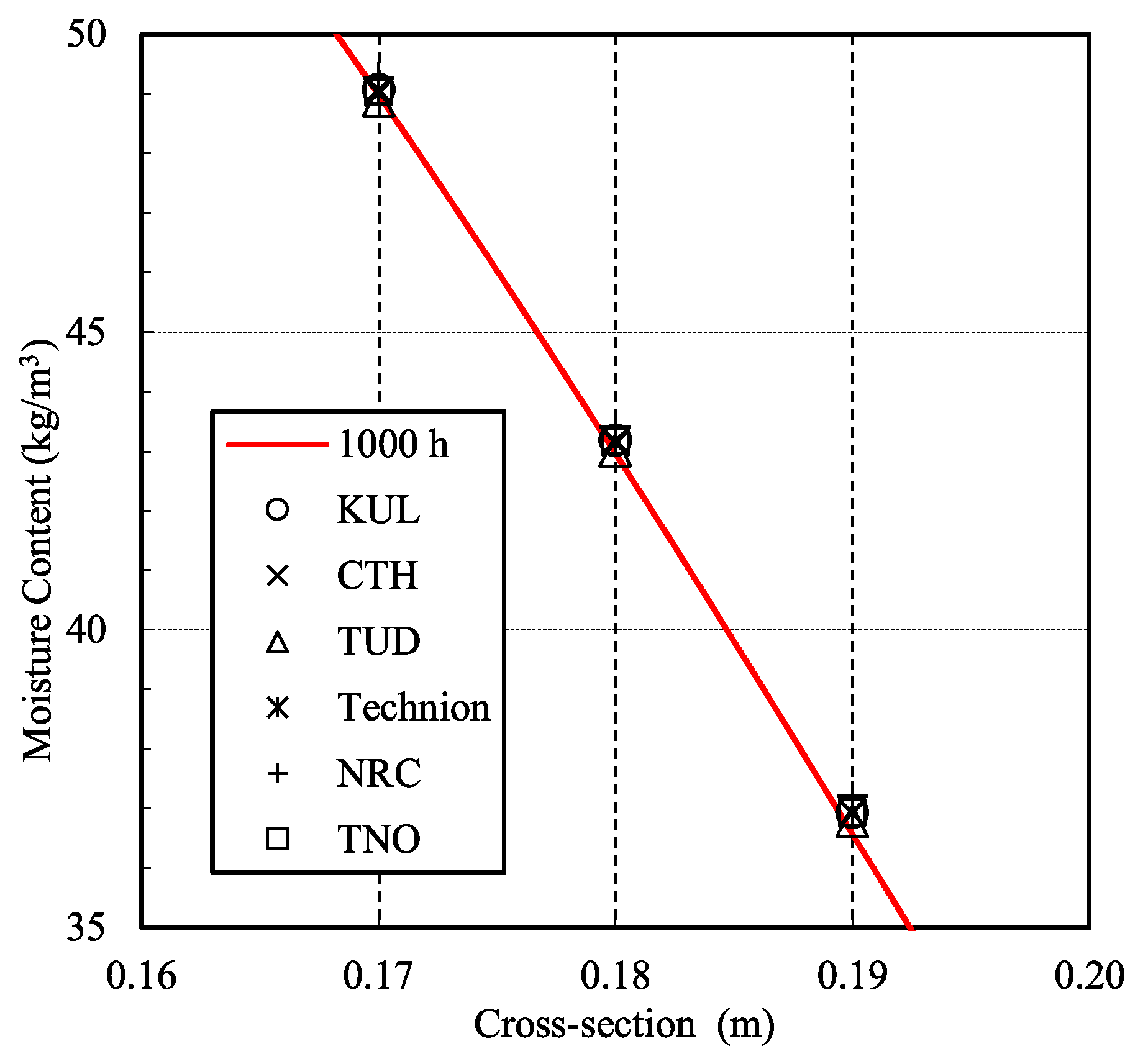
Due to the high numerical convergence and close quantitative agreement among the independent solutions provided by the institutes participating in the HAMSTAD benchmark, the global transient moisture profiles in Figure 4 exhibit substantial curve overlap. To resolve this visual density and enable a rigorous local inspection, detailed zoomed-in views of key drying intervals and critical boundary regions are presented in Figure 5, Figure 6 and Figure 7 for 100, 300, and 1000 h, respectively, as required by the protocol.

Figure 5. Detailed moisture content profiles at 100 h.

Figure 6. Detailed moisture content profiles at 300 h.

Figure 7. Detailed moisture content profiles at 1000 h.

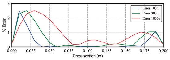
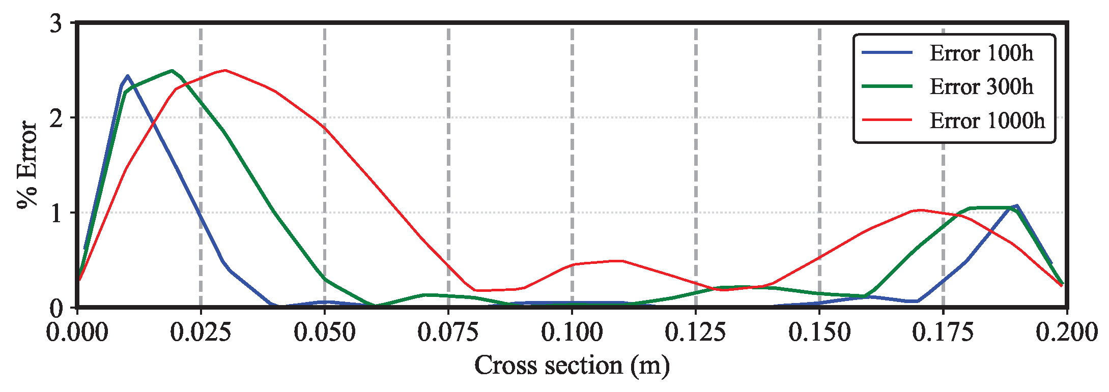
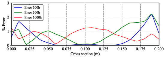
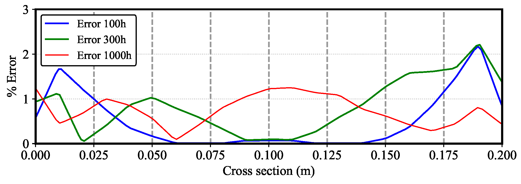
Figure 8 shows the error percentage when comparing the numerical results obtained using Dirichlet boundary conditions against the reference data from the HAMSTAD protocol.

Figure 8. Percentage error using Dirichlet boundary conditions.

Figure 9 shows the error percentage when comparing the numerical results obtained using Robin boundary conditions.

Figure 9. Percentage error using Robin boundary conditions.

A comparative error analysis between Figure 8 (Dirichlet) and Figure 9 (Robin) reveals distinct performance patterns. Under Dirichlet conditions, the relative error remains consistently under $0.8\%$ across the spatial domain because surface states are strictly fixed by algebraic boundary values. In contrast, under Robin convective boundary conditions, peak relative errors reach approximately $2.1\%$ during the initial drying stages ($t<100 \mathrm{h}$). This higher percentage error is attributed to two factors: (i) spatial discretization of the boundary half-cell ($\Delta x/2$), where first-order finite-difference approximations introduce truncation error into the convective flux balance $j_v={\beta }_p(P_{\mathrm{surf}}-P_{\mathrm{amb}})$, and (ii) the dynamic nonlinear interdependency between convective mass transfer coefficients and surface vapor depression, which amplifies gradient steepness near the surface boundary layer before steady drying kinetics are established.

To quantitatively evaluate the performance of our numerical model, a comparative statistical analysis was conducted against benchmark results from participants in the HAMSTAD protocol (Technion, KUL, CTH, TUD, NRC, and TNO). Model accuracy was quantified using the mean absolute error (MAE) and root mean square error (RMSE), expressed in ${\mathrm{kg}/\mathrm{m}}^3$.

The global statistical error metrics across $N=21$ spatial evaluation nodes are defined as:

$$\mathrm{MAE}={\displaystyle \frac{1}{N}}{\displaystyle \sum _{i=1}^N}\left|w_{i,\mathrm{num}}-w_{i,\mathrm{bench}}\right|,$$

(39)

$$\mathrm{RMSE}=\sqrt{{\displaystyle \frac{1}{N}}\sum _{i=1}^N{\left(w_{i,\mathrm{num}}-w_{i,\mathrm{bench}}\right)}^2},$$

(40)

where $w_{i,\mathrm{num}}$ and $w_{i,\mathrm{bench}}$ denote the numerical moisture content computed by our solver and the benchmark consensus solution at spatial node i, respectively.

Table 2 summarizes the MAE and RMSE values in ${\mathrm{kg}/\mathrm{m}}^3$ at three evaluation times ($100 \mathrm{h}$, $300 \mathrm{h}$, and $1000 \mathrm{h}$), where the best-performing values (lowest errors) for each time step and metric are highlighted in bold.

Table 2. Comparison of mean absolute error (MAE) and root mean square error (RMSE) in ${\mathrm{kg}/\mathrm{m}}^3$ across 100 h, 300 h, and 1000 h for six institutional models.

Institute	$\mathit{t}=100 \mathbf{h}$		$\mathit{t}=300 \mathbf{h}$		$\mathit{t}=1000 \mathbf{h}$
	MAE	RMSE	MAE	RMSE	MAE	RMSE
Technion	0.221	0.268	0.248	0.287	0.355	0.394
KUL	0.252	0.308	0.261	0.292	0.422	0.453
CTH	0.380	0.504	0.341	0.381	0.396	0.432
TUD	0.403	0.648	0.435	0.530	0.267	0.321
NRC	0.321	0.425	0.362	0.428	0.529	0.567
TNO	0.214	0.266	0.222	0.264	0.351	0.392

As observed in Table 2, the results indicate a remarkably low degree of overall variability among the participating institutions. Furthermore, the magnitude of these errors is physically negligible; for instance, average errors around $0.2 {\mathrm{kg}/\mathrm{m}}^3$ represent a relative error of less than 1% when compared to the characteristic scale of the target variable ($20–80 {\mathrm{kg}/\mathrm{m}}^3$). This confirms the high physical fidelity and robustness of the numerical simulations across all implementations. The subtle discrepancies observed across time steps reflect how each institute tackles the physical problem through distinct numerical formulations, spatial discretization schemes, or underlying modeling assumptions. Specifically, TNO achieves the highest accuracy at short- and mid-term evaluations ($100 \mathrm{h}$ and $300 \mathrm{h}$), whereas TUD demonstrates superior performance at $1000 \mathrm{h}$. Overall, our proposed model exhibits strong agreement with these leading benchmarks, demonstrating high predictive consistency and competitive accuracy throughout the entire simulation timeframe.

4.2. Results for Experimental Data and Physical Transport Mechanisms

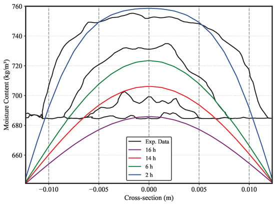
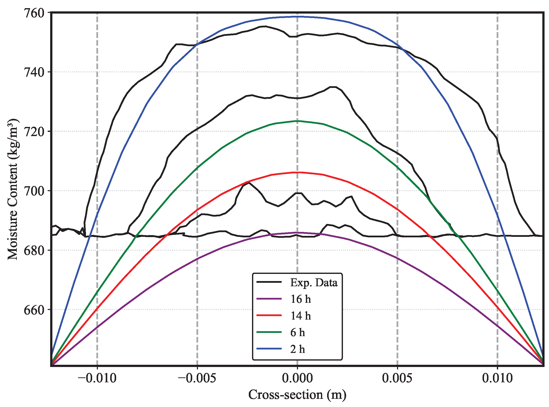
The numerical results are now compared with available experimental datasets reported by Schellen [12]. As clearly observable in Figure 10, the transient drying behavior is captured with high predictive fidelity across all temporal evaluations (2 h, 6 h, 14 h, and 16 h). This agreement can be interpreted through both physical transport mechanisms and numerical discretization characteristics.

Figure 10. Transient moisture content profiles across the specimen thickness: validation of the proposed computational code against experimental datasets reported by [12] at 2 h, 6 h, 14 h, and 16 h.

Specifically, the transient profiles display a clear, symmetrical reduction in moisture content over time, evolving from an initial high-moisture state at 2 h to a substantially flatter profile at 16 h. At the early stage of drying (2 h), the numerical solver captures the peak core moisture content with high precision. The steep moisture gradients observed near the external boundaries ($\left|x\right|>0.010 \mathrm{m}$) are governed by the Robin convective boundary condition, where boundary layer resistance regulates initial surface evaporation before internal transport becomes the primary rate-limiting step. In the bulk interior, liquid transport is driven by steep capillary suction pressure gradients ($\partial P_{\mathrm{suc}}/\partial w$).

As drying progresses through 6 and 14 h, the simulated parabolic curves accurately track the experimental decay. During these intermediate stages, as local moisture content decreases, internal transport gradually transitions from capillary liquid movement to vapor diffusion through air-filled lumens and bound-water diffusion within cell walls, driven by relative humidity gradients ($\partial \varphi /\partial x$).

The minor local fluctuations and subtle asymmetries present in the experimental NMR curves are attributed to natural anatomical heterogeneities of solid wood (e.g., density variations, annual ring orientation) and intrinsic NMR measurement noise, both of which are idealized in the homogeneous continuum formulation. By 16 h, both the simulation and experimental profiles converge toward a nearly uniform moisture distribution of approximately $685 {\mathrm{kg}/\mathrm{m}}^3$, confirming that the proposed FVM model reliably captures both short-term transient fronts and long-term equilibrium kinetics.

4.3. Influence of Model Simplifications and Physical Limitations

To maintain computational efficiency while adhering to the HAMSTAD Benchmark No. 2 protocol, certain secondary physical phenomena were neglected. Their physical influence on the model predictions is evaluated as follows.

• Thermal Coupling: In non-isothermal drying, temperature gradients induce thermo-diffusive fluxes (Soret effect) and enthalpy sinks due to phase change. However, for room-temperature or slowly conditioned timber elements, thermal equilibrium (${\tau }_{\mathrm{thermal}}\sim {10}^2\mathrm{s}$) is established several orders of magnitude faster than moisture equilibrium (${\tau }_{\mathrm{moisture}}\sim {10}^5\mathrm{s}$), validating the isothermal approximation.
• Sorption Hysteresis: Wood exhibits higher equilibrium moisture content during desorption than adsorption at equivalent relative humidity. Because primary timber drying follows a strictly monotonic desorption path, neglecting hysteresis introduces negligible error. Hysteresis modeling becomes essential primarily under cyclic environmental relative humidity boundary conditions.
• Shrinkage and Swelling: Below the fiber saturation point ($\mathrm{FSP}\approx 0.30\mathrm{kg}/\mathrm{kg}$), volumetric contraction reduces the physical diffusion path length by $3–8\%$. Neglecting spatial mesh contraction yields a slight, conservative overestimation of total drying time (<4%), which is acceptable for preliminary engineering design.

5. Conclusions

A problem-solving computational framework based on the HAMSTAD Benchmark No. 2 protocol was successfully developed to evaluate transient mass transfer in porous media using a fully implicit finite volume method (FVM). A primary innovative contribution of this study lies in the detailed numerical isolation and physical characterization of boundary condition dynamics. The discretized solver achieved strong quantitative agreement with analytical benchmark solutions, capturing transient diffusive profiles with a low average error of 5.8%, accompanied by high global precision as evidenced by low statistical error metrics ($\mathrm{MAE}<0.215 {\mathrm{kg}/\mathrm{m}}^3$ and $\mathrm{RMSE}<0.322 {\mathrm{kg}/\mathrm{m}}^3$). Crucially, the comparative analysis revealed distinct boundary-driven behaviors: while simulated surface behavior matched reference data over time, first-type (Dirichlet) conditions induced a clear discrepancy in core values due to the delayed penetration of boundary constraints, whereas third-type (Robin) conditions concentrated variations near surface nodes. These results align with established literature regarding the profound influence of boundary conditions on moisture transport in porous media.

Furthermore, the numerical algorithm was validated against real experimental data from solid wood drying, demonstrating high fidelity in capturing transient moisture content kinetics. From a practical standpoint, the developed tool offers strong potential to solve two core engineering problems:

• Drying Schedule Optimization. It provides the timber industry with a reliable predictive tool to estimate the exact drying time required for a material to reach a target moisture content, reducing energy consumption in industrial kilns.
• Hygrothermal Risk Assessment. It offers building physics engineers a computationally efficient model to evaluate localized transient moisture accumulation in structural timber elements under quasi-isothermal conditions.

From a physical perspective, experimental limitations were identified, as isothermal conditions were not fully guaranteed throughout the drying process, and nuclear magnetic resonance (NMR) measurements exhibited higher sensor uncertainty near lower moisture thresholds. Numerically, the primary limitation remains the uncoupled modeling of heat and moisture transfer. Incorporating explicit temperature dependence to refine this diffusional model and expanding the computational framework toward coupled multiphysics models represent the core directions for future development, as outlined in the Future Work Section.

Future Work

Future work will focus on expanding the computational capabilities of the proposed numerical framework in three main directions:

• Hygroscopic Hysteresis. Integrating distinct adsorption and desorption equilibrium isotherms to quantify the impact of moisture history on long-term hygrothermal predictions in structural timber elements.
• Full Thermo–Hygrometric Coupling. Advancing toward a fully non-isothermal formulation that accounts for the thermodynamic interdependencies between heat and moisture transport, explicitly capturing temperature-driven vapor diffusion and local latent heat sources and sinks induced by phase change within the porous matrix.
• Industrial Upscaling. Extending the computational solver from single wood specimens to the hygrothermal performance of entire multi-row lumber stacks subjected to convective drying in commercial kilns, incorporating localized boundary layer dynamics and microclimatic airflow variations across the stack geometry.

References

- Chen, H. Biotechnology of Lignocellulose; Springer: Dordrecht, The Netherlands, 2014. [Google Scholar] [CrossRef] [Scilit]
- Burdett, S.; Arora, M.; Myers, R.J. Sustainable materials selection with emerging structural materials. npj Mater. Sustain. 2026, 4, 13. [Google Scholar] [CrossRef] [Scilit] [PubMed]
- Lopez-Carreon, I.; Jahan, E.; Yari, M.H.; Esmizadeh, E.; Riahinezhad, M.; Lacasse, M.; Xiao, Z.; Dragomirescu, E. Moisture Ingress in Building Envelope Materials: (II) Transport Mechanisms and Practical Mitigation Approaches. Buildings 2025, 15, 762. [Google Scholar] [CrossRef] [Scilit]
- Zhang, Y.; Wang, X.; Liu, H. Computational fluid dynamics analysis for improving the uniformity of flow field in heat air drying kilns. Therm. Sci. 2024, 28, 825–834. [Google Scholar] [CrossRef] [Scilit]
- Livani, A.; Crivellaro, A.; Bosco, E. A 3D multi-scale hygro-mechanical model of oak wood. Wood Sci. Technol. 2023, 57, 1–42. [Google Scholar] [CrossRef] [Scilit]
- Younsi, R.; Kocaefe, D.; Poncsak, S.; Kocaefe, Y. Computational modelling of heat and mass transfer during the high-temperature heat treatment of wood. Appl. Therm. Eng. 2007, 27, 1424–1431. [Google Scholar] [CrossRef] [Scilit]
- Hagentoft, C.-E.; Kalagasidis, B.; Adl-Zarrabi, S.; Roels, S.; Carmeliet, J.; Hens, H.; Grunewald, J.; Funk, M.; Becker, R.; Shamir, D.; et al. Assessment Method of Numerical Prediction Models for Combined Heat, Air and Moisture Transfer in Building Components: Benchmarks for One-dimensional Cases. J. Therm. Envel. Build. Sci. 2004, 27, 327–352. [Google Scholar] [CrossRef] [Scilit]
- Patankar, S. Numerical Heat Transfer and Fluid Flow; Hemisphere Publishing Corporation: Washington, DC, USA, 1980. [Google Scholar]
- Maliska, C.R. Transferência de Calor e Mecânica dos Fluidos Computacional; LTC: Rio de Janeiro, Brazil, 1995. [Google Scholar]
- Eaton, J.W.; Bateman, D.; Hauberg, S.; Wehbring, R. GNU Octave (Version 11.1.0) [Software]. 2026. Available online: https://www.gnu.org/software/octave/ (accessed on 3 March 2026).
- Delgado, J.M.P.Q.; Barbosa de Lima, A.G. Transport Phenomena and Drying of Solids and Particulate Materials; Springer International Publishing: Cham, Switzerland, 2014. [Google Scholar]
- Schellen, H.L. Heating Monumental Churches: Indoor Climate and Preservation of Cultural Heritage. Ph.D. Thesis, Eindhoven University of Technology, Eindhoven, The Netherlands, 2002. [Google Scholar] [CrossRef]
- Philip, J.R.; De Vries, D.A. Moisture Movement in Porous Materials under Temperature Gradients. Trans. Am. Geophys. Union 1957, 38, 222–232. [Google Scholar] [CrossRef] [Scilit]
- Hagentoft, C.-E. HAMSTAD—Final Report: Methodology of HAM-Modeling; Chalmers University of Technology: Gothenburg, Sweden, 2002. [Google Scholar]
- Dos Santos, G.H.; Mendes, N. Heat, air and moisture transfer through hollow porous blocks. Int. J. Heat Mass Transf. 2009, 52, 2390–2398. [Google Scholar] [CrossRef] [Scilit]
- Mendes, N.; Chhay, M.; Berger, J.; Dutykh, D. Numerical Methods for Diffusion Phenomena in Building Physics; Springer: Cham, Switzerland, 2019. [Google Scholar]
- Press, W.H.; Teukolsky, S.A.; Vetterling, W.T.; Flannery, B.P. Numerical Recipes: The Art of Scientific Computing, 3rd ed.; Cambridge University Press: Cambridge, UK, 2007. [Google Scholar]
- Roels, S.; Carmeliet, J.; Hens, H. A Comparison of Different Techniques to Quantify Moisture Content Profiles in Porous Building Materials. J. Therm. Envel. Build. Sci. 2004, 27, 261–276. [Google Scholar] [CrossRef] [Scilit]
- Woodruff, W.F.; Revil, A. CEC-normalized clay-water sorption isotherm. Water Resour. Res. 2011, 47, W11502. [Google Scholar] [CrossRef] [Scilit]
- Tariku, F.; Kumaran, K.; Fazio, P. Transient model for coupled heat, air and moisture through multilayered porous media. Int. J. Heat Mass Transf. 2010, 53, 3035–3044. [Google Scholar] [CrossRef] [Scilit]
- Johnson, C.S., Jr. Diffusion ordered nuclear magnetic resonance spectroscopy: Principles and applications. Prog. Nucl. Magn. Reson. Spectrosc. 1999, 34, 203–356. [Google Scholar] [CrossRef] [Scilit]
Disclaimer/Publisher’s Note: The statements, opinions and data contained in all publications are solely those of the individual author(s) and contributor(s) and not of MDPI and/or the editor(s). MDPI and/or the editor(s) disclaim responsibility for any injury to people or property resulting from any ideas, methods, instructions or products referred to in the content. |
© 2026 by the authors. Licensee MDPI, Basel, Switzerland. This article is an open access article distributed under the terms and conditions of the Creative Commons Attribution (CC BY) license.