


Abstract
Conservation laws are core concepts in dynamical system modeling and the study of physical symmetries. Although machine learning has achieved significant progress in discovering physical laws, existing methods often face challenges such as identifying only a single conserved quantity. To bridge this gap, we introduce OAC-Net. By embedding a gradient orthogonality penalty directly into the neural network’s objective function, OAC-Net enables the simultaneous discovery of multiple independent integrals of motion (IOM) directly from raw trajectory data. Unlike previous heuristic approaches, we prove that gradient orthogonality of real-analytic functions implies the functional independence of the learned integrals of motion. The proposed method is validated on several canonical dynamical systems, including the two-dimensional Kepler system. Experimental results show that OAC-Net efficiently and robustly identifies multiple independent integrals of motion, with the learned integrals of motion exhibiting strong correlations with their true physical values. Additionally, ablation studies confirm OAC-Net’s robustness to hyperparameters such as noise strength and orthogonal penalty coefficient. Our approach provides an effective framework for discovering multiple interpretable integrals of motion from complex trajectory data.
1. Introduction
Within the research framework of system modeling, conserved quantities in dynamical systems constitute one of the central and indispensable concepts. They not only provide profound insights into the symmetry properties of system structures, but also offer essential theoretical support for the in-depth investigation of low-dimensional embedding characteristics [1]. In many cases, conserved quantities even serve as the unique state descriptors of chaotic dynamical systems [2]. With the remarkable advances in big data technologies and machine learning, a growing body of research has employed machine learning techniques to address theoretical problems in physics, including the identification of phase transitions [3,4], astronomical observations [5], and the simulation of quantum systems [6,7]. Consequently, the methodological paradigm of “discovering physical laws from data” has achieved substantial progress. Following this line of research, the present study employs machine learning approaches to automatically uncover conservation laws of dynamical systems directly from trajectory data.
Before surveying these methods, we fix the terminology. Following Landau and Lifshitz [8] and AI Poincaré 2.0 [9], we call a smooth function that is constant along every trajectory an integral of motion (IOM), and we reserve the term conservation law for those IOMs that stem from the spacetime symmetries of the system and exhibit additivity. Neural networks trained without such inductive biases naturally parameterize IOMs rather than conservation laws. The physical conservation laws form a distinguished subset of the IOMs, and this distinction will be used throughout the paper.
Noether’s theorem establishes a fundamental connection between conservation laws and the symmetries of physical systems. In practice, physicists often exploit symmetry principles to derive conservation laws in a model-driven manner. For instance, Poincaré demonstrated that the three-dimensional gravitational three-body problem admits only ten conserved quantities by invoking spatial translational and rotational symmetries, as well as translational symmetries in time and Galilean transformations [10]. Nevertheless, in many situations it remains difficult to obtain exact conservation laws or even to determine their number. In this context, machine learning provides a data-driven avenue for inferring Hamiltonians and conservation laws directly from observations. Broadly speaking, machine learning approaches for discovering conservation laws can be classified into two categories. The first category infers the Hamiltonian through explicit functions [11]; however, such methods typically rely on approximate surrogate models constructed from approximate functions such as polynomial functions, and thus can only recover simplified approximations of the true dynamics. The second category employs deep learning techniques to model Hamiltonians or conservation laws, as exemplified by the works of Bondesan and Lamacraft [12], Greydanus et al. [13], and Toth et al. [14]. Arora et al. [15] proposed a machine learning framework for ordinary differential equations based on the skew-gradient form and the discrete gradient method. By designing three strategies for learning multiple first integrals, their approach is able to recover the first integrals of a system solely from trajectory data, and, as a byproduct, infer the underlying ordinary differential equations that generate the data. In addition, Wetzel et al. [16] introduced Siamese neural networks into theoretical physics and applied them to scenarios such as special relativity and electromagnetism. By interpreting the bottleneck layer via polynomial regression, they addressed the longstanding issue of limited interpretability in neural networks. Ha and Jeong [1] innovatively constructed a noise-variance loss function and proposed the ConservNet neural network, which was applied to synthetic systems, the Volterra equation, and the Kepler problem, among others. Their method overcomes the reliance on data preprocessing and the lack of robustness inherent in traditional approaches. However, a common limitation shared by the above two classes of neural-network-based methods is that, even when multiple conserved quantities exist, the models are typically able to identify only a single one. Mototake [17], grounded in Noether’s theorem, modeled the manifold structure of time-series data using deep autoencoders. By combining replica-exchange Monte Carlo (REMC) sampling to infer dynamical symmetries, they subsequently extracted the corresponding conservation laws. Liu and Tegmark [18] proposed the AI Poincaré algorithm, which automatically determines the number of conserved quantities from trajectory data of unknown dynamical systems through Monte Carlo manifold sampling and PCA-based dimensionality estimation. They validated the method on five dynamical systems, including the harmonic oscillator. However, this approach relies on the assumption of trajectory ergodicity and is unable to provide any information beyond the number of conserved quantities. Building upon this work, Liu et al. [9] introduced the AI Poincaré 2.0 method, incorporating the concepts of differentiable rank and differentiable independence. Starting from the differential equations of dynamical systems, they parameterized conservation laws with neural networks, enabling the discovery of all conserved quantities and their numerical evaluation without requiring the ergodicity assumption. Nevertheless, due to the inherent smoothness of neural networks, AI Poincaré 2.0 struggles to learn ill-behaved conserved quantities and still faces difficulties in uncovering symbolic expressions for complex conservation laws. To address the limited interpretability of deep-learning-based approaches, Liu et al. [19] proposed the Sparse Invariant Detector (SID). Also based on differential equations, SID operates within a conservation-law basis-function framework specified by human experts and enforces sparsity on the coefficient vectors, thereby achieving greater interpretability and yielding symbolic expressions for conservation laws. Taken together, the neural-network methods reviewed above exhibit a clear division of labor. Methods that rely solely on trajectory data determine either only the number of conservation laws (AI Poincaré 1.0 [18]) or only the numerical form of a single conserved quantity (ConservNet [1] and the Siamese networks [16]), whereas methods that recover multiple independent laws [9,17,19] rely on additional information, such as the governing differential equations or human-specified basis functions and transformation families. The problem of simultaneously determining the number of conservation laws and recovering the numerical form of each independent law from raw trajectory data alone has therefore remained open for neural-network approaches.
Figure 1 illustrates our overall workflow. To fill this gap, the present study introduces OAC-Net (Ortho-AIPoincare-ConserNet), which combines two classes of neural networks in succession that are employed to determine the number of conservation laws and to estimate the numerical forms of each conserved quantity, respectively. For the numerical identification of conservation laws, ConservNet [1] represents a simple yet robust approach. By means of the innovative Noise-Variance Loss Function, it enables the learning of neural-network-parameterized conserved quantities while preventing convergence to trivial constant functions. However, ConservNet and Siamese neural networks [16] share a common limitation: even when a system possesses multiple conserved quantities, they are typically capable of identifying only a single one. To overcome this drawback, the present work proposes a novel integration of the AI Poincaré family of methods [9,18]. Specifically, AI Poincaré 1.0 is first employed to infer the number of conservation laws embedded in the trajectory data, thereby determining the number of neural networks required to parameterize the conserved quantities. Subsequently, a gradient orthogonality loss term is incorporated into the Noise-Variance Loss Function to enforce the mutual independence of the learned conservation laws.
Figure 1.
Overall Workflow of OAC-Net.
For clarity, the components adopted from the three methods above and the novel contributions of this paper are summarized as follows. From AI Poincaré 1.0 [18], OAC-Net adopts the trajectory-based manifold-sampling module that determines the number n of conservation laws, and uses it without modification. From ConservNet [1], OAC-Net adopts the noise-variance loss as the objective for learning the numerical form of a conserved quantity, and extends it from a single law to n separate networks, one per law. From AI Poincaré 2.0 [9], OAC-Net adopts the idea of separating parameterized conservation laws through their gradients, but replaces its implementation, which requires the governing differential equations, with a penalty on the pairwise inner products of the normalized gradients of the n networks, computed by automatic differentiation from trajectory data alone. The novel contributions of this paper are therefore the gradient orthogonality penalty together with its theoretical justification, namely the theorem that gradient orthogonality of real-analytic functions implies their functional independence, and the resulting pipeline that recovers the number and the numerical form of every independent law from raw trajectory data without governing equations or human-specified priors.
2. Determination of the Number of Conservation Laws
Strictly speaking, the dimension of the trajectory manifold determines the number of independent integrals of motion in the terminology of the Introduction. We keep the term conservation laws in this section for readability.
The determination of the number of conservation laws benefits from the progress of machine-learning-based manifold sampling [20]. Sampling manifolds are closely related to dynamical systems: each state of a dynamical system can be regarded as a point in the phase space , and the topological closure of the set of all states along a trajectory forms a manifold . Each conservation law partitions the original N-dimensional phase space into a family of level sets. Consequently, a single conservation law removes one degree of freedom from the dynamical system. Therefore, the number of conservation laws is given by the difference between the dynamical system dimension N and the dimension of the trajectory manifold , namely [21]. For a dynamical system defined by , suppose that its conservation laws are given by , . The corresponding state manifold is defined as . It is then evident that the number of conservation laws equals . However, the trajectory set does not constitute the complete state manifold. In fact, if the system is ergodic, then is everywhere dense in , implying that . In this case, the number of conservation laws can be expressed as .
An assumption underlies this counting procedure. The observed trajectories must be ergodic, or at least sufficiently diverse, so that the trajectory set is dense in the state manifold. If this assumption is violated, since the closure of the observed trajectory set is contained in the state manifold, the estimated manifold dimension becomes smaller than the true one, and the estimated number of integrals is correspondingly overestimated. The extra integrals are then local to the observed trajectories rather than global conservation laws, as the Lagrangian three-body experiment in the Section 6 illustrates. AI Poincaré 2.0 makes the same point about the original algorithm, noting that the ergodicity assumption was tacit in AI Poincaré 1.0 and that systems such as the KdV equation violate it [9]. In all our experiments we therefore generate trajectories from multiple level sets.
For a dense subset of a state manifold formed by noise-free samples, the manifold dimension is equal to the rank of the sample covariance matrix in an infinitesimal neighborhood of a randomly selected sample point [18], under which the manifold can be approximated by a hyperplane. In practice, however, only a finite number of data points are available, making it impossible to access infinitesimal neighborhood information. To address this issue, AI Poincaré 1.0 [18] estimates the data manifold dimension through a combination of prewhitening, local Monte Carlo sampling, and PCA explained-ratio estimation. Specifically, in the prewhitening step, an affine transformation is applied to the sample points such that the trajectory data have zero mean and an identity covariance matrix, while dimensions corresponding to vanishing eigenvalues are removed. These eigenvectors represent linear conserved quantities. Prewhitening improves the isotropy of the manifold, making its radius of curvature as similar as possible across different directions [18]. Subsequently, the Monte Carlo manifold sampling procedure consists of a “Walk” step and a “Pull” step. In the “Walk” step, isotropic Gaussian noise with zero mean and covariance matrix is added to a state vector , where L is noise scale and is the identity matrix, so that each component of the perturbation is an independent Gaussian variable with variance L, yielding a perturbed state vector . In the subsequent “Pull” step, a feedforward neural network with parameters is trained to map the perturbed state vector back toward the original state manifold, with the loss function defined as:
where denotes the number of samples. Since a neural network can at most project perturbed points orthogonally onto the data manifold, once an appropriate noise scale L is chosen, the pulled-back points can be used to characterize the local tangent space of the manifold [18,20]. Finally, principal components of the pulled-back points are computed under different noise scales L. At certain intermediate noise scales L, some principal components decrease to values close to zero and are identified as sub-manifold structures, each of which corresponds to a conservation law. By counting the number of principal components whose explained variance ratios fall below the threshold at such a noise scale, one can determine the number of conservation laws associated with the dynamical system. The threshold is the isotropic baseline of the prewhitened data: after prewhitening, the trajectory data have an identity covariance matrix, so every unstructured direction carries an expected explained variance ratio of , and a principal component that falls below this baseline is compressed relative to isotropy and is identified as a sub-manifold structure. This criterion is adopted from AI Poincaré 1.0, where it was validated against ground truth on five systems including the two-dimensional Kepler problem and the two-dimensional three-body problem [18]. The estimated count is insensitive to the exact threshold value. If the threshold were raised above the baseline, noise-driven components could be misidentified as sub-manifold structures and the count would be biased upward. If it were lowered toward the noise floor, genuine sub-manifold components could be missed and the count would be biased downward. Within the wide band between the noise floor and the baseline, the count remains unchanged, and the chosen value sits at the upper edge of this band. The explained-ratio valley is well separated from the baseline in our experiments, because the data are generated analytically without observation noise and are densely sampled.
3. Determination of Numerical Values of Individual Independent Conservation Laws
Many studies have employed neural networks to fit conservation laws, such as the AI Poincar’e 2.0 method proposed by Liu et al. [9]. This approach starts from the differential equation and parameterizes the conservation law H using a neural network. A loss function is then constructed based on the property that the dot product between the gradient of a conserved quantity and the vector field vanishes, namely . However, in practical trajectory data, the governing equations satisfied by the trajectories are generally unknown, and real-world data are often contaminated by substantial noise. In fact, a conservation law can be interpreted as a constant-valued function of the state vector: it does not vary with time. That is, its values at any sample points should be identical, or at least the variance of its values across all sample points should be minimized. To satisfy this criterion, the loss function of the neural network should include a variance term over its outputs at all sample points, namely , where denotes the conservation law parameterized by the neural network. However, using a single variance term as the loss function is highly likely to cause the network to converge to a trivial constant function, i.e., a solution for which the output remains a fixed constant regardless of the input samples and is entirely independent of the state variables. Such a result is clearly meaningless. In practice, adding an input-augmentation term with noisy perturbations to the variance term can effectively suppress this trivial convergence, leading to a loss function of the form:
where Q denotes the spreading constant, denotes the variance over the sample index j within each trajectory, and represents a random noise vector subject to the constraint . The parameters Q and R jointly control the diffusion resolution.
However, neural networks designed in this manner are only capable of discovering a single conserved quantity, even when multiple conservation laws are present in the system [1]. Nevertheless, employing a variance term together with a noise-augmented input expansion as the loss function provides a valuable paradigm for parameterizing conservation laws using neural networks. As established in Section 2, the number of conservation laws in the dynamical system has already been determined and is denoted by n. In principle, one may parameterize the n conservation laws using n separate neural networks, each trained with the loss function given in Equation (2). However, this strategy may lead all networks to converge to the same conserved quantity or to highly correlated ones, whereas distinct conservation laws are expected to be mutually independent. Liu et al. [9] introduced an independence loss based on the inner products of gradients of different conserved quantities, successfully identifying mutually orthogonal conservation laws. Following a similar idea, we incorporate an orthogonality loss term into the overall loss function. Consequently, the total loss function of OAC-Net is given by:
where denotes the penalty coefficient of the orthogonality loss, and represents a normalized gradient vector.
To judge whether the learned laws are mutually independent, we use the following direct measure introduced by AI Poincaré 2.0 [9].
Definition 1.
For non-zero differentiable functions on an open set , form the matrix
whose p-th row is the gradient of . The differential rank of the function set is , and the set is differentially independent if holds on a dense open subset of Ω.
By the chain rule, a differentiable relation forces to vanish at every point where has full rank, and conversely, rank deficiency on a nonempty open set produces a local relation after straightening, so the two notions of independence agree. The case of this definition is restated as Definition A1 in the appendix. Numerically, the rank is computed by the singular value decomposition of B at a finite set of sample points, counting the singular values whose explained fraction of the total squared singular value sum exceeds , which is the threshold convention of AI Poincaré 2.0 [9]. A finite set of random sample points is exponentially unlikely to underestimate the differential rank. In the Section 6 this measure is applied to the trained networks on held-out test trajectories.
AI Poincaré 2.0 already enforces independence during training through a pairwise orthogonality regularization on the normalized gradients of the networks, and it additionally uses the differential rank as a post-training screening tool, computing it by singular value decomposition after training [9]. The reason the rank itself cannot serve as a training objective is that it is a non-differentiable functional of the network parameters, piecewise constant with vanishing gradient almost everywhere, whereas the sum of squared inner products of the normalized gradients is smooth and trainable, and pairwise orthogonality of nonzero vectors implies full rank. OAC-Net adopts both mechanisms, the training-time orthogonality penalty of Equation (3) and the post-training rank screening of Definition 1, the latter being used in this paper as a post-training validation measure on test trajectories, in the same role as in AI Poincaré 2.0. The difference from AI Poincaré 2.0 lies in the conservation objective that accompanies the orthogonality penalty. AI Poincaré 2.0 minimizes the equation-based term , which requires the governing equations, whereas OAC-Net minimizes the noise-variance loss, so that the entire pipeline, the orthogonality penalty included, is computed from raw trajectory data alone.
4. Construction and Training of Neural Networks
OAC-Net consists of two neural networks: the classical AI Poincaré 1.0 comprises four-layer feedforward fully connected neural networks, where both the input layer and the output layer are N-dimensional vectors (N denotes the dimensionality of the system’s state space). The two hidden layers each contain 256 neurons, with SiLU [22] employed. AI Poincaré1.0 generates sampling points on the local manifold by learning the projection of the noisy point onto the original manifold, and subsequently utilizes ERD to automatically identify the number of conserved quantities. The ConservNet has an input dimension of N, an output dimension of 1, contains four hidden layers, and adopts the MISH activation function [23]. Both aforementioned neural networks are trained using the ADAM optimizer [24] from PyTorch [25]. The random noise vectors are randomly sampled from a multivariate uniform distribution, where each noise component is independent and subject to the regularization constraint . By default, the hyperparameters R, Q, and in all our experiments are set to 1, and the robustness of OAC-Net to these hyperparameters is validated in Appendix C. The complete training configuration of the two stages is summarized in Table 1. All experiments were run on a single NVIDIA RTX 5090 GPU with 32 GB of memory, using PyTorch 2.8.0 with fp32 precision and four processes in parallel. Under the training configuration of Table 1, one complete training run takes 1.7 min for the circular system and 22 min for the two-dimensional three-body problem in measured wall-clock time, and at most about 8.5 min and 8.4 min for the two-dimensional isotropic harmonic oscillator and the two-dimensional Kepler problem, respectively, where the latter two values are conservative upper bounds extrapolated from the measured per-step rate.
Table 1.
Training configuration of OAC-Net.
5. Dataset
In this study, OAC-Net was evaluated on circular trajectories, the two-dimensional Kepler system, the two-dimensional isotropic harmonic oscillator, and three-body motion. During training, data were sampled alternately from multiple trajectories lying on distinct level sets of the conserved quantities. Experimental observations indicate that for systems possessing only a single conservation law, such as the circular trajectory system, OAC-Net is capable of discovering the conserved quantity using data from a single trajectory. However, for systems with multiple conservation laws, such as the two-dimensional Kepler system, training on a single trajectory makes OAC-Net highly prone to learning several overfitted neural networks. These overfitted networks are typically characterized by an extremely low output variance along the training trajectory, yet exhibit significant fluctuations in their outputs when evaluated on trajectories with different values of the conserved quantities within the same class of dynamical systems. To facilitate the validation of experimental results, we fixed certain parameters during data generation and generated target trajectory data by specifying a particular conserved quantity (e.g., the radius for circular trajectories, the energy for the isotropic harmonic oscillator). To validate the performance of the model on real-world datasets, we utilize the official database provided by the NASA Jet Propulsion Laboratory (JPL), which contains sub-arcsecond precision orbital data for all planets, satellites, asteroids, and comets in the Solar System. This database provides comprehensive information, including position and velocity vectors at any given epoch (for details, see https://ssd.jpl.nasa.gov/). Specifically, we employ the trajectory data of the eight major planets in the Solar System for training. The Observer Location is set to the Solar System Barycenter (SSB). The data spans from 15 March 2000 to 15 March 2026, with a time step of one day. Distances are measured in Astronomical Units (AU), and the X-Y plane is defined as the ecliptic plane of Earth’s orbit (specifically the J2000.0 heliocentric mean ecliptic coordinate system).
The data construction methodology for each experiment is detailed in Appendix A. The code is available at: (https://github.com/Willian-JT-Shen/OAC-Net, accessed on 25 July 2026).
6. Results
For each simulated system, we prepared trajectory datasets consisting of 1000 sample points for trajectories with radii (or total energies) of 0.01, 1, 4, 9, and 16. This constitutes a relatively small data volume compared to other contemporary deep learning studies [16,17,18]. For each trained network, we performed testing on a total of 1608 trajectories with radii (or total energies) ranging from 0.01 to 16, using a step size of 0.01. Each of these test trajectories also contained 1000 sample points.
The performance of OAC-Net was evaluated using the following two metrics: firstly, we examined whether the output variance along each test trajectory remained low. Secondly, we computed the mean output value for each test trajectory, which serves as the value of the conserved quantity learned by OAC-Net for that corresponding trajectory. Subsequently, we compared these mean values with the true conserved quantities for each test trajectory by computing the correlation coefficient.
To evaluate the performance of OAC-Net, we first conduct tests on circular trajectories, as shown in Figure 2. Figure 2c presents a bar plot with error bars illustrating OAC-Net’s output variance on each test trajectory of the circular system. The bar height represents the mean output variance of OAC-Net across samples within a given test trajectory, while the error bars indicate the standard deviation of the output variance. These results demonstrate that OAC-Net maintains consistently low output variance across trajectories within the system, exhibiting high stability. To examine the similarity between OAC-Net and the ground-truth conservation laws, we visualize the ground-truth conserved quantities and the corresponding numerical outputs of OAC-Net for each trajectory, as shown in Figure 2e,f. Additionally, we computed the mean output value for each test trajectory, which serves as the value of the conserved law learned by OAC-Net for that corresponding trajectory. In Figure 2d, the horizontal axis represents the ground-truth conservation law for each circular trajectory—specifically, the radius of the circular orbit—while the vertical axis denotes the values predicted by OAC-Net across trajectories of varying radii. The correlation coefficient between the ground-truth conservation laws and the OAC-Net outputs is in the default seed-42 run shown in Figure 2d; averaged over ten random seeds the correlation is (Table 2), indicating that OAC-Net effectively captures the underlying conservation laws.
Figure 2.
Identifying the conserved energy for circular trajectory. (a) The circular trajectory has 2 degrees of freedom: positions x and y. (b) Sample trajectories illustrate sampling points in the 2D phase space. The color represents the radius of the circular trajectories. (c) The output variance of conservation law in the circular trajectory demonstrates that the model maintains low output variance across the majority of trajectories and exhibits minimal inter-trajectory variability in its variance levels. (d) The horizontal and vertical axes represent the ground-truth conservation laws and the values of the model output, respectively. The two variables exhibit a predominantly linear relationship, with a correlation coefficient of (seed 42; ten-seed average in Table 2). (e,f) illustrate the performance of the ground-truth conservation laws and the learned conservation laws across all trajectories, respectively. The color scale indicates the magnitude of the conservation law values.
Table 2.
Mean and standard deviation of the main metrics over ten random seeds.
However, a discrepancy in the scale ranges of the horizontal and vertical axes is observable. Notably, this does not signify a model deficiency. Rather, it reflects an inherent characteristic of conservation laws: they can effectively distinguish differences between trajectories but are inherently difficult to map to an absolute numerical value. For a Hamiltonian system governed by the ordinary differential equation , a conserved quantity is defined as a scalar function satisfying [9]. Consequently, any single-valued function of the conservation law is also a conserved quantity, as . Nevertheless, under the Noise-Variance constraint (2), the linear form of the conservation law emerges as the optimal solution for the model [1], which accounts for the inconsistent ranges between the axes in Figure 2d. Although the raw output of OAC-Net does not provide absolute numerical values, the scaling factor and intercept can be determined via linear calibration when the ground-truth law is known. Furthermore, for systems where the ground truth is unknown, symbolic regression methods can be directly applied to the model output to extract the analytical expression of the conservation law, allowing the scaling coefficients to be identified from the ratios of the terms’ coefficients.
To evaluate the performance of OAC-Net in more complex dynamical systems, we applied the model to a 2D isotropic harmonic oscillator, as illustrated in Figure 3a. The sampled trajectories used for this analysis are presented in Figure 3b. Following the analytical approach used for the circular trajectories, we calculated the output variance of the conservation laws and the correlation coefficients between the mean output values and the ground-truth conserved quantities for the 2D isotropic harmonic oscillator, as shown in Figure 3c and Figure 3d, respectively. Figure 3e–g visualize the values of the x-energy, y-energy, and angular momentum along the sampled trajectories, while Figure 3h–j display the corresponding outputs from the three OAC-Net components. During testing, Output1 and Output3 of OAC-Net maintained a consistently low output variance across all test trajectories. In contrast, Output2 exhibited a higher mean output variance, a finding further corroborated by Figure 3i. Despite the inability of Output2 to maintain low variance across different trajectories, Figure 3i indicates that OAC-Net successfully captured the characteristic “vortex-like” distribution of the conservation laws inherent in the 2D isotropic harmonic oscillator. This is further evidenced by the fact that Output2 significantly outperforms Output1 in Figure 3d, with Output3 achieving the highest fidelity in learning the conservation laws among the three. However, the correlation matrix in Figure 3d shows identical data for each row, suggesting that the three ground-truth conservation laws exhibit identical behavior across the test trajectories. In fact, the high degree of symmetry between the x and y directions in both the training and testing trajectories leads to the uniform performance of the three conservation laws in the 2D isotropic harmonic oscillator system, as detailed in Table 3. This symmetry poses a significant challenge for the symbolic regression of analytical expressions for these laws. Nevertheless, the gradient orthogonality term in the OAC-Net loss function effectively ensures that the identified conservation laws satisfy functional independence, even under these highly symmetric conditions.
Figure 3.
Identifying the conserved energy for 2D isotropic Harmonic Oscillator. (a) The 2D isotropic Harmonic Oscillator system also has 4 degrees of freedom: positions x, y and velocities , . (b) Sample trajectories illustrate sampling points in the 2D phase space. The color scale corresponds to the energy levels of the orbits. (c) The output variance of conservation law in the 2D isotropic Harmonic Oscillator system suggests that the model achieves consistently low output variance for most trajectories, characterized by minimal cross-trajectory fluctuations in variance. (d) The mean output values are compared with true conserved quantities by calculating the correlation coefficient in each test trajectory. (e–j) visualize the ground-truth versus model-predicted conservation laws across all trajectories, with the color scale reflecting the magnitude of the respective conserved quantities.
Table 3.
Conservation Law in Each System.
To investigate the performance of OAC-Net in identifying conservation laws containing radial functional terms, we applied the model to the 2D Kepler problem, as illustrated in Figure 4a. The sampled trajectories for this system are presented in Figure 4b, where the interpretation of each subfigure follows the same convention as that of the 2D isotropic harmonic oscillator. Generally, in the study of dynamical systems involving radial components, researchers often manually incorporate radial terms into the system rather than requiring the neural network or symbolic search to directly fit complex square-root expressions. This practice significantly reduces the difficulty of functional fitting for the neural network [9]. However, in our evaluation, we did not pre-include radial terms as input variables for the network. As demonstrated by Output1 in Figure 4e, our model is nonetheless capable of effectively learning conservation laws that contain radial dependencies.
Figure 4.
Identifying the conserved energy for 2D Kepler Conservation. (a) The 2D Kepler system has 4 degrees of freedom: positions x, y and velocities , . (b) Sample trajectories illustrate sampling points in the 2D phase space. The trajectories are color-coded according to their orbital energy levels. (c) The output variance of conservation law in the 2D Kepler system indicate that the model’s output variance remains consistently low across most trajectories, with low discrepancy in variance between different trajectories. (d) The mean output values are compared with true conserved quantities by calculating the correlation coefficient in each test trajectory. (e–j) depict the distributions of the ground-truth and model-identified conservation laws over all trajectories respectively, where the color mapping represents the values of the respective conservation laws.
To evaluate the performance of OAC-Net on systems with higher degrees of freedom and a greater number of conservation laws, we further investigated its behavior in the 2D Three-body Problem, as illustrated in Figure 5a. For both training and testing, we utilized the Lagrangian solution of the three-body problem, characterized by three bodies of equal mass maintaining a constant, equilateral triangle configuration while undergoing uniform circular motion about the barycenter. Due to the inherent symmetry of this configuration, we present the trajectory of only one representative body in Figure 5b.
Figure 5.
Identifying the conserved energy for 2D three-body problem. (a) The 2D three-body problem also has 12 degrees of freedom: positions , , , , , and velocities , , , , , . (b) Sample trajectories illustrate sampling points in the 2D phase space. Since we focus on the Lagrangian solution, where three bodies are positioned at the vertices of an equilateral triangle and undergo identical circular motion about the barycenter, only the trajectory of a single body is plotted here for brevity. The color scale corresponds to the energy levels of the orbits. (c) While the majority of models demonstrate robust performance on the test set by maintaining low variance levels, certain models exhibit significant performance variability across different trajectories. (d) Initial experiment of the 2D three-body problem. The model performs poorly in learning the momentum components in the x-direction and y-direction. To explore the reason of the phenomenon, we conduct a further experiment with more generalized and diverse trajectory training data in (e).
Notably, a total of 11 conserved quantities were identified in the three-body problem, whereas physicists generally recognize only four conserved laws in this system [9]. This discrepancy arises because OAC-Net actually identifies integrals of motion (IOM), rather than conserved laws in the strict sense. In fact, integrals of motion are the fundamental elements that partition the phase space into time-invariant submanifolds [26], whereas conserved laws are those IOM that adhere to spacetime symmetries and exhibit additivity [8]. Physically meaningful integrals of motion must be globally defined and smooth across the entire phase space [26].
In fact, within the three-body problem in Figure 5d, the first two parameterized neural networks can effectively reflect the system’s total energy and angular momentum, respectively. However, OAC-Net performs poorly in learning the momentum components in the x-direction and y-direction. Theoretically, even though the physical conserved laws of the three-body problem constitute only 4 out of the 11 integrals of motion, it should not be the case that none of our 11 parameterized neural networks successfully learns the x-direction and y-direction momentum. This outcome may stem from the specific nature of the datasets employed, as well as the inherent limitations of the Noise-Variance term within the loss function. The Noise-Variance term typically prioritizes conservation laws characterized by steeper gradients and wider numerical ranges—such as angular momentum in this context. This preference is quantified in the appendix. Consequently, multiple outputs within the OAC-Net framework tend to collectively converge toward the conserved quantity with the dominant gradient, as illustrated in Figure 5d. Furthermore, to facilitate deducing the state vector of the corresponding trajectory from the system’s total energy, we assumed the solution corresponds to Lagrangian points, where the three bodies have equal masses and perpetually maintain an equilateral triangle configuration. This assumption introduces additional integrals of motion that are local (i.e., specific to the Lagrangian solution): (1) The distances between each pair of bodies remain constant: . (2) The speeds of each body are equal: . (3) The distance from each body to the center of mass (located at the origin): . (4) The angular momentum of each body is constant: . (5) The radial velocity of each body is zero. Since the three bodies undergo uniform circular motion around the center of mass (origin), their direction of motion is always perpendicular to their position vectors, i.e., purely tangential motion: . (6) The potential energy of the system is constant, as the inter-body distances remain invariant: . (7) The kinetic energy of the system is constant, as the speeds of the bodies remain unchanged: . This classification can be made precise with the help of the manifold dimension. Along the Lagrangian family the closure of the observed trajectory set has dimension 1, so the counting stage returns independent integrals, which agrees with the general fact discussed in AI Poincaré 2.0 [9] that a first-order system with s degrees of freedom admits local integrals of motion. Among these 11, the four integrals that are additive and stem from the spacetime symmetries of the system are the global conservation laws. The remaining seven are local to the Lagrangian family. Each describes a distinct constraint imposed by the equilateral configuration, namely the constancy of the pairwise distances, of the individual speeds, of the distances to the center of mass, of the individual angular momenta, of the radial velocities, of the potential energy, and of the kinetic energy, and each fails to extend to the full phase space because it presupposes that configuration. The independence of the 11 integrals is guaranteed by the dimension count, while the list above serves as an illustration rather than as an independent basis. This is the same distinction between local and global constants made in AI Poincaré 2.0 under the name of Frobenius integrability.
When the diversity and generality of the training trajectory data are increased, as shown in Figure 5e, OAC-Net is indeed capable of effectively uncovering the four target conservation laws of the Three-Body Problem, while successfully escaping the local optima associated with dominant gradients.
Two observations make this failure mechanism precise. First, on the Lagrangian family the center of mass is fixed at the origin, so the total momentum vanishes identically on the data. A law that is identically zero on the data provides no in-data variation for the variance term of the noise-variance loss, so it is invisible to the optimizer, while laws with rich in-data variation, such as the angular momentum, are captured first. Second, the diversity of the data can be diagnosed operationally before and after training. Before training, an estimated count of signals that the closure of the trajectory set has dimension 1, namely that the data consist of a single orbit family, since is precisely the local count of integrals along a single trajectory in the sense of Frobenius integrability. After training, the differential rank of Definition 1 can be evaluated on held-out trajectories, and a differential rank below the number of trained networks indicates duplicated or degenerate laws. In our experiments the restricted Lagrangian data trigger the first signal, with an estimated count of 11, while the diverse data restore the four target laws. We therefore recommend that users generate trajectories from several distinct level sets and verify both signals. However, given the interpretability of physical meaning, applying OAC-Net to unknown systems still poses the challenge of discerning physically meaningful conservation laws from among multiple model outputs.
In fact, these additional local constants of motion are mathematically well-posed. As Thirring pointed out, one can always find time-independent constants of motion along a local trajectory of a mechanical system with n degrees of freedom; however, not all of these local constants can be continuously extended to the entire phase space [26]. This underscores the necessity of employing trajectory data that are as diverse as possible when training OAC-Net.
To determine the contribution of the orthogonality term, we performed an ablation study in which the term was removed by setting , while all other settings remained identical, and we compared the two variants on the four major systems with ten random seeds each, using paired t-tests. On every multi-law system, removing the term significantly degrades the orthogonality of the learned gradients on held-out test trajectories, as summarized in Table 4. The mean pairwise inner product of the normalized gradients increases by a factor of 2.7 on the two-dimensional isotropic harmonic oscillator (), by a factor of 4.3 on the two-dimensional Kepler problem (), and by a factor of 21 on the two-dimensional three-body problem (), as shown in Figure 6. The output cross-correlations increase correspondingly on the harmonic oscillator and on the Kepler problem, and they are already high on the three-body problem in both variants. By contrast, the conservation accuracy is statistically indistinguishable between the two variants, and the circular system, for which the orthogonality term is inactive by construction since only one law is learned, shows identical results under both settings. These results confirm that the orthogonality term is solely responsible for the functional independence of the learned laws and does not trade off against accuracy.
Table 4.
Mean pairwise inner product of the normalized gradients on held-out test trajectories, with and without the orthogonality term, over ten seeds.
Figure 6.
Ablation of the gradient orthogonality term. (a) Comparison of the full model and the ablation model on the four systems. (b) Distribution of the pairwise normalized gradient inner products on held-out test trajectories. The stars in (a) denote the significance level of the paired t-test (*** means ).
To address the sensitivity of the training procedure to random initialization, we repeated all main experiments with ten random seeds and report the mean and the standard deviation of the main metrics in Table 2. The effective rank is recovered identically in every run for all four systems, namely 1 for the circular system, 3 for the two-dimensional isotropic harmonic oscillator and the two-dimensional Kepler problem, and 11 for the two-dimensional three-body problem, which shows that the number of learned laws is insensitive to the random seed. The accuracy correlation is also stable across seeds, with coefficients of variation between 2.2 percent and 8.1 percent. The test variance and the gradient inner product show larger variation across seeds, but their means remain at the levels reported in the main text.
We further tested OAC-Net under noisy observations of the trajectories. Gaussian noise of level , measured as a fraction of the per-component standard deviation of the clean training set, is injected into the training trajectories only, at levels , across all four systems with five random seeds each, while the test trajectories remain clean. The conservation accuracy degrades by less than 10% for on every system. Even at the strong noise level , the two-dimensional Kepler problem and the two-dimensional three-body problem retain and respectively, the circular system remains above at every noise level, and the isotropic oscillator is essentially unaffected, with a slight improvement consistent with a regularizing effect of the noise. The gradient inner products on held-out test trajectories remain essentially constant across all noise levels, as shown in Figure 7, which confirms that the orthogonal structure enforced during training is robust to noisy observations. We note that the observation noise introduced here is a data-quality issue, distinct from the input perturbation in the loss of Equation (3), which is an algorithmic component of OAC-Net.
Figure 7.
Conservation laws recovered by OAC-Net under observation noise. (a) Accuracy versus the noise level . Each curve shows the mean best-match correlation between the learned quantities and the ground-truth laws on clean test trajectories over five seeds, with error bars denoting ± one standard deviation. (b) Mean pairwise normalized gradient inner products on held-out test trajectories versus the noise level .
To address the gap between the exact orthogonality assumed by the theorem of the appendix and the approximate penalty that is actually minimized during training, we recorded the orthogonality term of Equation (3) at every epoch for all four systems over ten random seeds each, as shown in Figure 8. On every multi-law system the penalty decreases monotonically from its random-initialization value of order one to the level, with final values for the two-dimensional isotropic harmonic oscillator, for the two-dimensional Kepler problem, and for the two-dimensional three-body problem, while for the circular system with a single law it is identically zero by construction. The dashed lines mark the Gershgorin threshold derived in the appendix, below which the Jacobian of the learned laws is guaranteed to have full rank, and the converged values lie one to two orders of magnitude below the threshold on every multi-law system. The trained networks are therefore almost exactly orthogonal on the training distribution, which connects the approximate penalty to the exact orthogonality assumed by the theorem.
Figure 8.
Training dynamics of OAC-Net on the four benchmark systems (, 2000 epochs, solid line = mean over ten random seeds, shaded band = one standard deviation). Top row = total loss of Equation (3), bottom row = orthogonality term . Dashed line = Gershgorin threshold , which equals for the two four-dimensional systems and for the three-body system.
Finally, to validate the performance of the model on real-world datasets, we applied our method to a subset of trajectory data from the eight major planets in the Solar System as a case study on real observational data. Existing frontier research in parameterized conservation law identification exhibits several limitations. One class of methods is restricted to identifying only a single conservation law within multi-conserved systems, such as ConservNet [1] and SNN [16]. In these approaches, identifying multiple laws requires generating a new dataset while holding the first discovered law constant—a procedure that is often impractical for real-world applications. Another class of methods relies heavily on human prior knowledge to identify multiple conservation laws, such as AI Poincaré 2.0 [9], SID [19], and DeepEncoder [17]. Specifically, AI Poincaré 2.0 and SID require the system’s differential equations to be known a priori. SID further necessitates the input of basis functions by human experts, while DeepEncoder requires a predefined family of candidate transformation functions. This case study relies on the standard approximation that each planet moves in the central gravitational field of the Sun, so that inter-planetary perturbations, which are much smaller than the solar term for the eight major planets, are neglected, and each planetary orbit is treated as a three-dimensional Kepler problem in the barycentric frame, whose independent conserved quantities are the five listed in Table 5. Trained on the eight planetary trajectories, OAC-Net recovers five independent integrals, and Figure 9 shows the result. Panel a is a schematic representation of the eight planetary orbits, and panel b shows the correlation matrix between the five outputs of OAC-Net and the five ground-truth quantities listed in Table 5. Each quantity is captured by a distinct output, namely the energy by the fourth output, the x-component and the y-component of the momentum by the second and the fifth outputs, the z-component of the momentum by the first output, and the x-component of the Runge-Lenz vector by the third output. The correlation is strong for each of these pairs but below one, while the remaining outputs correlate weakly with that quantity. The deviation from perfect correlation is expected, since each output is one diffeomorphic image of the corresponding true law, and the linear representative is obtained only after an appropriate change in variables, as discussed in the Conclusion. Together with the small size of this dataset, which consists of eight trajectories, this gauge freedom explains the imperfect correlation visible in panel b, and the results support the use of the JPL data as a sanity check for the method on real, high-precision observational data. A quantitative comparison with other methods on this dataset is left to future work, since the source code of the skew-gradient approach is not publicly available, the OT-Manifold method requires on the order of one hundred trajectories, which the Solar System does not provide, and the remaining methods operate in different settings, as discussed above. The experiment was performed on a single NVIDIA RTX 5090 GPU with fp32 precision, using the training configuration of Table 1.
Table 5.
Independent Conservation Law in Solar System.
Figure 9.
Conserved quantities recovered from JPL Solar System data. (a) Schematic representation of the eight major planets in the Solar System. (b) The mean output values of OAC-Net compared with the true conserved quantities by correlation coefficients on each test trajectory.
7. Conclusions
We propose OAC-Net, a neural-network-based approach for the automated identification of conservation laws. We evaluated our method across a diverse range of dynamical systems, including circular trajectories, the 2D Kepler problem, the 2D isotropic harmonic oscillator, and the 2D three-body problem. Furthermore, as a case study on real observational data, we applied OAC-Net to the JPL orbital data of the eight major planets in the Solar System. On these data the outputs of OAC-Net are approximately linear transformations of the ground-truth conserved quantities, up to the gauge freedom discussed in the Section 6.
Despite its advantages, OAC-Net still faces certain limitations, such as computational inefficiency. Furthermore, as discussed in the context of the 2D three-body problem, the number of integrals of motion identified often exceeds the number of physically meaningful conservation laws, necessitating a further screening process of the model’s outputs. In the terminology fixed in the Introduction, the physical conservation laws are the subset of the recovered integrals of motion that are characterized by spacetime symmetry and additivity, and identifying this subset is precisely the screening step mentioned above.
We emphasize that the goal of OAC-Net is to provide candidate expressions for the integrals of motion of the system, rather than to single out the physical conservation laws automatically. The relation between the two is nevertheless constructive. Any smooth function of a conserved quantity is again an integral of motion, and, conversely, when a learned output is functionally dependent on a true law, the true law is obtained from the output by a change in variables, namely by a local diffeomorphism wherever the gradient of the output does not vanish. The candidate integrals of motion recovered by OAC-Net therefore provide a coordinate system in which the physical conservation laws, characterized by symmetry and additivity, are one diffeomorphism away. Selecting the representative with the desired physical properties, for example through symbolic regression on the learned outputs or through the inductive biases of AI Poincaré 2.0 [9], is a downstream step that we leave to domain knowledge, as illustrated for the systems of Table 3 by the correlation analysis in the Section 6. Several potential strategies may be employed to address these challenges. One approach involves human scientists proposing basis functions for conserved quantities based on the specific problem context and subsequently sparsifying the coefficient vectors of these basis functions to enhance interpretability [19]. Another approach entails incorporating inductive biases, such as spacetime symmetries and additivity, into the conserved quantities [9]. In practice, both methodologies require human scientists to provide problem-specific prior knowledge, underscoring that machine learning models cannot entirely replace human scientists. Indeed, as Liu et al. [19] articulates, the role of machine learning methods is not to supplant human scientists, but rather to address technical and tedious tasks, thereby enabling human scientists to focus more intently on creative endeavors.
Two properties of the method deserve explicit statement. First, the recovery of the full set of laws relies on the diversity of the observed trajectories, as the three-body experiment shows, and the manuscript provides two operational checks for this condition, the pre-training count of the manifold dimension and the post-training differential rank on held-out trajectories. Second, the theoretical support of the method is exactly the following chain. Theorem A1 proves that exact gradient orthogonality of real-analytic functions implies functional independence, the quantitative bound of the appendix extends this statement to the approximate empirical penalty by showing that residual pairwise inner products below the threshold still guarantee full rank of the gradient matrix, and the training dynamics of Figure 8 show that the trained networks indeed converge below this threshold, with the full rank verified independently on held-out test trajectories in Table 2. What the theory establishes is therefore the sufficiency of the orthogonality mechanism, and what the experiments verify is that the trained networks satisfy the conditions of the theory.
Author Contributions
Conceptualization, J.S. and D.L.; methodology, J.S. and D.L.; software, J.S.; validation, J.S. and D.L.; formal analysis, J.S. and D.L.; investigation, J.S.; resources, D.L.; data curation, J.S.; writing—original draft preparation, J.S.; writing—review and editing, D.L.; visualization, J.S.; supervision, D.L.; project administration, D.L.; funding acquisition, D.L. All authors have read and agreed to the published version of the manuscript.
Funding
This research received no external funding.
Institutional Review Board Statement
Not applicable.
Informed Consent Statement
Not applicable.
Data Availability Statement
The original contributions presented in this study are included in the article. The source code is available at https://github.com/Willian-JT-Shen/OAC-Net (accessed on 25 July 2026). Further inquiries can be directed to the corresponding author.
Conflicts of Interest
The authors declare no conflicts of interest.
Appendix A. Construction of Experimental Data
Appendix A.1. Circular Trajectory Data
For a circle in the two-dimensional Cartesian coordinate system with center at and radius R, the trajectory equation is given by:
In fact, the above equation is equivalent to the parametric form , , where . For simplicity and convenience, we assume , allowing us to readily construct trajectory data based on the radius R.
Appendix A.2. Two-Dimensional Kepler Data
The two-dimensional Kepler motion represents a typical elliptical orbit problem. The position coordinates of the orbiting body can also be expressed in polar coordinates: , where is the true anomaly. Provost et al. [27], based on the discrete-time concept and deriving from polar coordinates, obtained the expressions and , from which the polar equation of the elliptical orbit can be derived as
where a is the semi-major axis and e is the eccentricity. Consequently, the coordinates of the orbiting body along the trajectory can be expressed as:
Furthermore, Provost et al. [27] presented an explicit expression for the velocity in the same article: . We take the constant vector to be along the y-axis, i.e., , and express the transverse unit vector as a function of , , and : , where is the unit vector along the positive x-axis and is the unit vector along the positive y-axis. Consequently, the velocity expression can be rewritten as:
Given that , we further obtain , where , G is the gravitational constant, and M is the mass of the central body. Therefore, the velocity of the orbiting body can be expressed as:
The Vis-viva equation [28] explores the relationship between energy and the semi-major axis.
Consequently, we can specify the energy E of the two-dimensional Kepler system, and subsequently determine the state vector equation via the semi-major axis a:
Appendix A.3. Two-Dimensional Isotropic Harmonic Oscillator
We derive the state vector of the trajectory starting from the total energy of the system. For a given total energy E, assuming the allocation ratio of the total energy between the x- and y-directions is , then the energies in the two directions are given by and , respectively. In fact, the energies in the x- and y-directions can be expressed analytically as and , and when , the harmonic oscillator system is isotropic [9], in which case angular momentum is conserved. For simplicity, we assume . Since the state vector is given by the following expression [9]:
Then, substituting the state vector expression into the total energy yields:
where and denote the amplitudes in the x- and y-directions, respectively. It then follows that
Given the preceding assumptions of uniform energy distribution between the x and y-directions, i.e., , coupled with the isotropy condition , the state vector can be ultimately expressed as follows:
In practice, one can generate a set of state vectors for an isotropic harmonic oscillator trajectory with a specified total energy E by randomly sampling the initial phases from the interval .
Appendix A.4. Generation of State Vectors for the Lagrangian Solution of the Three-Body Problem
To facilitate deriving the state vector from the total energy and constructing trajectories with varying energies, we make the following assumptions: (1) The three bodies have equal masses, set to unity, i.e., ; (2) The gravitational constant G is set to unity; (3) The center of mass of the system is fixed at the origin; (4) The solution corresponds to the Lagrangian points, meaning the three bodies always form an equilateral triangle, and the entire triangle rotates around the center of mass with a constant angular velocity . We derive the displacements and velocities of the three bodies in the x and y directions starting from the total energy of the three-body problem. The total energy of the system comprises kinetic energy and potential energy, where the potential energy is the sum of the gravitational potential energies between each pair of bodies. Thus, the total potential energy is . In the Lagrangian solution of the three-body problem, the side length L of the equilateral triangle and the angular velocity satisfy [29]. The speed can be expressed as . Consequently, the kinetic energy can be written as . Therefore, the total energy is , from which we can derive the side length of the equilateral triangle starting from the total energy: . The speed can then be expressed as . It is worth noting that in the three-body problem, the energy is negative. Thus, in the Lagrangian solution of the three-body problem, we only need to specify the total energy E of the system; the side length L of the equilateral triangle and the rotational speed v are then determined, and consequently, the displacements and velocities of the three bodies in the x and y directions are also established.
Appendix B. Proof of the Independence of the Learnt Conservation Laws
Ha and Jeong [1] have demonstrated that, under the assumption of a single conserved quantity, employing as the loss function causes the optimal solution of the neural network to converge to a constant function. They further proved that the noise variance loss , upon the introduction of a noise term, guides the network to learn nontrivial, input-dependent conserved quantities. However, constructing neural networks directly with the aforementioned loss function makes it prone to learning highly correlated conserved quantities [9]. Ideally, we desire the multiple learned conserved quantities to be functionally independent in the sense of Definition A1 below. In fact, we point out that the orthogonality of gradients of functions constitutes a sufficient condition for functional independence. Accordingly, we propose the following theorem:
Definition A1.
Non-constant functions , where is a nonempty open connected set and denotes the class of real-analytic functions, are said to be functionally independent if for every the relation for all implies that f is identically zero on .
Remark A1.
A point is called a regular point if and , otherwise it is called a critical point, and the critical set is denoted . An equivalent differential formulation requires that the Jacobian matrix have rank 2 at every point of a dense open subset of Ω. The equivalence between the two formulations is classical for real-analytic functions, and the chain-rule argument is spelled out in Definition 1 of Section 3, of which the present definition is the case .
Theorem A1.
For non-constant functions , in , where is a nonempty open connected set and , if gradients of and are orthogonal, i.e.,
then they are functionally independent, i.e., for every the relation for every implies that f is identically zero on .
Proof.
Since holds for every , the partial derivative of with respect to is zero, i.e.,
where and . Given that the gradients of and are orthogonal, taking the dot product of both sides of Equation (A13) with yields:
Since the non-constant , each critical set is a proper analytic subvariety of . Therefore they have empty interior and measure zero, and so does their union S. On , we have and , so we obtain and in . By the continuity of and and the density of in , we have and pointwise in . Consequently, we have on the connected set , so is constant on , and because , this constant has to be zero. That is, f vanishes on the image . At any point of the nonempty open set , the gradients are nonzero and orthogonal, and therefore they are linearly independent, so the Jacobian of has rank 2. By the constant rank theorem [30], maps a neighborhood of that point onto an open subset of , thus f vanishes on a nonempty open subset of . Since f is real-analytic, the identity theorem yields on . □
The theorem above concerns exact orthogonality, whereas OAC-Net enforces orthogonality only through a finite penalty, so it remains to explain how small a residual penalty suffices. Let denote the normalized gradients of the n trained networks at a data point , and suppose the pairwise inner products satisfy for all . Form the matrix U with rows , and let be its Gram matrix. The diagonal entries of G equal 1 and the off-diagonal entries are bounded by , so by the Gershgorin circle theorem every eigenvalue of G lies in the interval . Hence , and if the Gram matrix is positive definite, so the vectors are linearly independent, and since each is a positive scalar multiple of , the gradient matrix of Definition 1 has full rank n at . Since , the residual penalty of the orthogonality term controls the smallest singular value of the normalized gradient matrix from below, and any below the threshold guarantees differential functional independence in the sense of Definition 1 at the point . For the two-dimensional three-body problem with trained networks the threshold is , and the mean pairwise inner product reported in Table 2 lies well below this threshold, as do the converged penalty values of the training dynamics shown in Figure 8.
Therefore, the gradient orthogonal term effectively ensures that the multiple non-constant neural networks governed by the noise variance loss exhibit good functional independence.
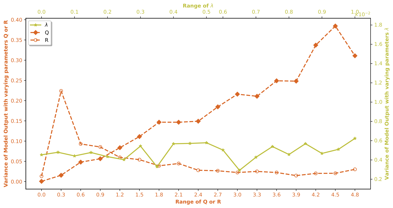
Appendix C. Robustness of OAC-Net to Hyperparameters R, Q, and
To investigate the influence of the parameters , Q, and R on OAC-Net performance, we varied the values of these three parameters in the two-dimensional isotropic harmonic oscillator system and computed the average output variance of each conserved quantity learned by OAC-Net under each configuration. During the experiments, only one parameter was varied at a time, while the other two were kept at their default value of 1. The lower and upper bounds for Q and R were set to 0 and 5, respectively, with a step size of 0.3. For , the lower and upper bounds were 0 and 1, respectively, with a step size of 0.05. The experimental results in Figure A1 demonstrate that OAC-Net exhibits strong robustness to the gradient orthogonal term parameter and the noise perturbation strength R. When the penalty intensity for gradient orthogonality is low, OAC-Net may still learn conserved quantities. However, these learned quantities are likely to lack functional independence. Gradually increasing the orthogonal penalty strength encourages the learned conserved quantities to span a maximally large space within the normal space of the manifold. Without significantly affecting the characteristic of the conserved quantities themselves, the output maintains low variance along the trajectories. Increasing the noise perturbation strength R generally does not substantially impact the average output variance of OAC-Net. Under relatively low noise strengths (e.g., 0.3 and 0.6), the average output variance of OAC-Net is comparatively high. This observation suggests that the noise strength should ideally not be less than the diffusion constant Q. Low noise intensity results in small differences between noisy data and original data. The Noise-Variance loss term forces the output variance of noisy data to match the diffusion constant Q. Consequently, the model maintains a similar variance level even for original data. This causes the model to learn excessive noise. This phenomenon is further corroborated by the degradation in model performance as the diffusion constant Q increases. When the actual noise strength is weaker than Q, OAC-Net will be forced to learn extraneous noise components, consequently interfering with model’s performance. These observations are consistent with the quantitative analysis below, in which the regime forces the network to inflate its gradients along the noise directions of the data, so the high output variance observed at small R is the signature of this failure direction, and the natural default is the choice . The choice of the gradient orthogonal term parameter offers greater flexibility. Although this sweep was performed on the two-dimensional isotropic harmonic oscillator, the behavior of the orthogonality term on systems of different dimensions and with different numbers of conservation laws is verified by the ablation study of Figure 6 and Table 4, by the training dynamics of Figure 8, by the ten-seed results of Table 2, and by the noise study of Figure 7, all of which cover the four systems up to the twelve-dimensional three-body problem with eleven learned laws.
Figure A1.
Robustness of OAC-Net to hyperparameters R, Q, and (on 2D isotropic Harmonic Oscillator).
The empirical behavior above follows from a second order expansion of the spreading term. Write , , and . The isotropic perturbation satisfies , , and its odd moments vanish. Expanding H at gives
The mean of this expansion is
where , the cubic part of the remainder has vanishing expectation by symmetry, and the remaining terms are . The second moment requires the fourth moment of the perturbation, and for a Gaussian spreader Isserlis’ theorem gives
The three Kronecker delta terms are the three possible pairings of the four indices into two covariances. The third pairing contributes , using the symmetry of the Hessian. Squaring the Taylor expansion and taking expectations, with H denoting , gives
where , the odd third order cross moment vanishes, and all terms involving the cubic remainder contribute . Squaring the mean gives
Subtracting the last two expressions, the terms, the terms, and the terms all cancel, and only the gradient and curvature contributions remain
The remainder absorbs the remaining contributions of order , in particular the cross term between the linear part and the cubic part of the expansion. The factor in front of the Frobenius term comes from the Gaussian fourth moment, and for any other isotropic symmetric spreader only the coefficient of changes by a constant of order one, which is absorbed in the remainder. The parameter depends on the radius distribution, since the constraint bounds the squared norm of every perturbation while its average satisfies . Averaging over the data points, the spreading constraint therefore calibrates the average gradient magnitude of the learned function to
This explains both failure directions. If , the required gradient magnitude exceeds the natural gradient of the physical laws, and the only directions in which the network can realize such large gradients are the noise directions of the data, so the network learns noise. If , the required gradient magnitude falls below the natural one, and the output degenerates toward a nearly constant function. Since the ground-truth laws have gradients of order one on standardized data, comparable values of R and Q provide a system-independent default, which is the choice used in this paper.
For a system that is unknown to the researcher, we recommend the following procedure. First, standardize the input components, which absorbs the system-specific scales. Second, choose R and Q of the same order, such as , as in this paper. Third, verify the choice with the checks available in the method, namely that the output variance along trajectories stays close to Q, and that the differential rank and the gradient inner products of the learned laws are healthy.
The same expansion quantifies the bias of the noise-variance loss toward conserved quantities with steeper gradients and wider numerical ranges, a preference already noted in ConservNet [1] and in the three-body discussion of the Section 6. The bias has two sources. First, the spreading constraint calibrates the average gradient magnitude of the learned function to , so a candidate law whose natural gradients lie well below this level can satisfy the constraint only after inflating its gradients, and inflation is realized along the noise directions of the data, whereas a law whose natural gradients lie well above this level must shrink them and degenerates toward a nearly constant function. Laws with steeper gradients therefore satisfy the spreading constraint at their natural scale and are occupied first during training. Second, the variance term of Equation (2) produces a gradient signal only for outputs that vary along the observed trajectories. A law that vanishes identically on the data, such as the total momentum on the Lagrangian family of the three-body problem, is invisible to this term, while laws with a wider numerical range provide the strongest signal and are captured first. The overall output scale is absorbed by the freedom to rescale H, so the residual preference is determined by the cross-trajectory mismatch , where is the mean squared gradient on the i-th training trajectory and is the output scale, and by the early training dynamics, rather than by the absolute gradient scale. Three controls tested in this paper reduce the bias to a preference over the recovery order rather than over the final set, the calibration of the robustness study above, the trajectory diversity of the three-body experiment, and the orthogonality penalty of the ablation study together with the rank screening of Table 2.
References
- Ha, S.; Jeong, H. Discovering invariants via machine learning. Phys. Rev. Res. 2021, 3, L042035. [Google Scholar] [CrossRef] [Scilit]
- Lu, P.Y.; Dangovski, R.; Soljačić, M. Discovering conservation laws using optimal transport and manifold learning. Nat. Commun. 2023, 14, 4744. [Google Scholar] [CrossRef] [Scilit] [PubMed]
- Carrasquilla, J.; Melko, R.G. Machine learning phases of matter. Nat. Phys. 2017, 13, 431–434. [Google Scholar] [CrossRef] [Scilit]
- Van Nieuwenburg, E.P.; Liu, Y.H.; Huber, S.D. Learning phase transitions by confusion. Nat. Phys. 2017, 13, 435–439. [Google Scholar] [CrossRef] [Scilit]
- Hezaveh, Y.D.; Levasseur, L.P.; Marshall, P.J. Fast automated analysis of strong gravitational lenses with convolutional neural networks. Nature 2017, 548, 555–557. [Google Scholar] [CrossRef] [Scilit] [PubMed]
- Baldi, P.; Sadowski, P.; Whiteson, D. Searching for exotic particles in high-energy physics with deep learning. Nat. Commun. 2014, 5, 4308. [Google Scholar] [CrossRef] [Scilit] [PubMed]
- Pang, L.G.; Zhou, K.; Su, N.; Petersen, H.; Stöcker, H.; Wang, X.N. An equation-of-state-meter of quantum chromodynamics transition from deep learning. Nat. Commun. 2018, 9, 210. [Google Scholar] [CrossRef] [Scilit] [PubMed]
- Landau, L.D.; Lifshitz, E.M. Mechanics, 3rd ed.; Pergamon Press: Oxford, UK, 1976; Chapter 2. [Google Scholar]
- Liu, Z.; Madhavan, V.; Tegmark, M. Machine learning conservation laws from differential equations. Phys. Rev. E 2022, 106, 045307. [Google Scholar] [CrossRef] [Scilit] [PubMed]
- Poincaré, H. Les Méthodes Nouvelles de la Mécanique Céleste; Gauthier-Villars et Fils: Paris, France, 1893; Volume 2. [Google Scholar]
- Schmidt, M.; Lipson, H. Distilling free-form natural laws from experimental data. Science 2009, 324, 81–85. [Google Scholar] [CrossRef] [Scilit] [PubMed]
- Bondesan, R.; Lamacraft, A. Learning symmetries of classical integrable systems. arXiv 2019, arXiv:1906.04645. [Google Scholar]
- Greydanus, S.; Dzamba, M.; Yosinski, J. Hamiltonian neural networks. In Proceedings of the Advances in Neural Information Processing Systems 32 (NeurIPS 2019), Vancouver, BC, Canada, 8–14 December 2019. [Google Scholar]
- Toth, P.; Rezende, D.J.; Jaegle, A.; Racanière, S.; Botev, A.; Higgins, I. Hamiltonian Generative Networks. In Proceedings of the 8th International Conference on Learning Representations, ICLR 2020, Addis Ababa, Ethiopia, 26–30 April 2020. [Google Scholar]
- Arora, S.; Bihlo, A.; Brecht, R.; Holba, P. Model-agnostic machine learning of conservation laws from data. arXiv 2023, arXiv:2301.07503. [Google Scholar]
- Wetzel, S.J.; Melko, R.G.; Scott, J.; Panju, M.; Ganesh, V. Discovering symmetry invariants and conserved quantities by interpreting siamese neural networks. Phys. Rev. Res. 2020, 2, 033499. [Google Scholar] [CrossRef] [Scilit]
- Mototake, Y.I. Interpretable conservation law estimation by deriving the symmetries of dynamics from trained deep neural networks. Phys. Rev. E 2021, 103, 033303. [Google Scholar] [CrossRef] [Scilit] [PubMed]
- Liu, Z.; Tegmark, M. Machine learning conservation laws from trajectories. Phys. Rev. Lett. 2021, 126, 180604. [Google Scholar] [CrossRef] [Scilit] [PubMed]
- Liu, Z.; Sturm, P.O.; Bharadwaj, S.; Silva, S.J.; Tegmark, M. Interpretable conservation laws as sparse invariants. Phys. Rev. E 2024, 109, L023301. [Google Scholar] [CrossRef] [Scilit] [PubMed]
- Saremi, S.; Hyvärinen, A. Neural empirical bayes. J. Mach. Learn. Res. 2019, 20, 1–23. [Google Scholar] [CrossRef] [Scilit]
- Goldstein, H.; Poole, C.; Safko, J. Classical Mechanics; Addison-Wesley: Reading, MA, USA, 1980. [Google Scholar]
- Elfwing, S.; Uchibe, E.; Doya, K. Sigmoid-weighted linear units for neural network function approximation in reinforcement learning. Neural Netw. 2018, 107, 3–11. [Google Scholar] [CrossRef] [Scilit] [PubMed]
- Misra, D. Mish: A Self Regularized Non-Monotonic Activation Function. In Proceedings of the 31st British Machine Vision Conference 2020, BMVC 2020, Virtual, 7–10 September 2020; BMVA Press: Durham, UK, 2020. [Google Scholar]
- Kingma, D.P.; Ba, J. Adam: A Method for Stochastic Optimization. In Proceedings of the 3rd International Conference on Learning Representations, ICLR 2015, San Diego, CA, USA, 7–9 May 2015. Conference Track Proceedings 2015. [Google Scholar]
- Paszke, A.; Gross, S.; Massa, F.; Lerer, A.; Bradbury, J.; Chanan, G.; Killeen, T.; Lin, Z.; Gimelshein, N.; Antiga, L.; et al. Pytorch: An imperative style, high-performance deep learning library. In Proceedings of the Advances in Neural Information Processing Systems 32 (NeurIPS 2019), Vancouver, BC, Canada, 8–14 December 2019. [Google Scholar]
- Harrell, E.M.; Thirring, W. A Course in Mathematical Physics 1 and 2: Classical Dynamical Systems and Classical Field Theory; Springer: New York, NY, USA, 1991. [Google Scholar]
- Provost, J.P.; Bracco, C. A simple derivation of Kepler’s laws without solving differential equations. Eur. J. Phys. 2009, 30, 581–586. [Google Scholar] [CrossRef] [Scilit]
- Logsdon, T. Orbital Mechanics: Theory and Applications; John Wiley & Sons: New York, NY, USA, 1997. [Google Scholar]
- Scheeres, D.J. Relative equilibria in the spherical, finite density three-body problem. J. Nonlinear Sci. 2016, 26, 1445–1482. [Google Scholar] [CrossRef] [Scilit] [PubMed]
- Whitney, H. Differentiable manifolds. Ann. Math. 1936, 37, 645–680. [Google Scholar] [CrossRef] [Scilit]
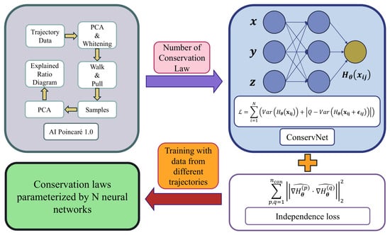
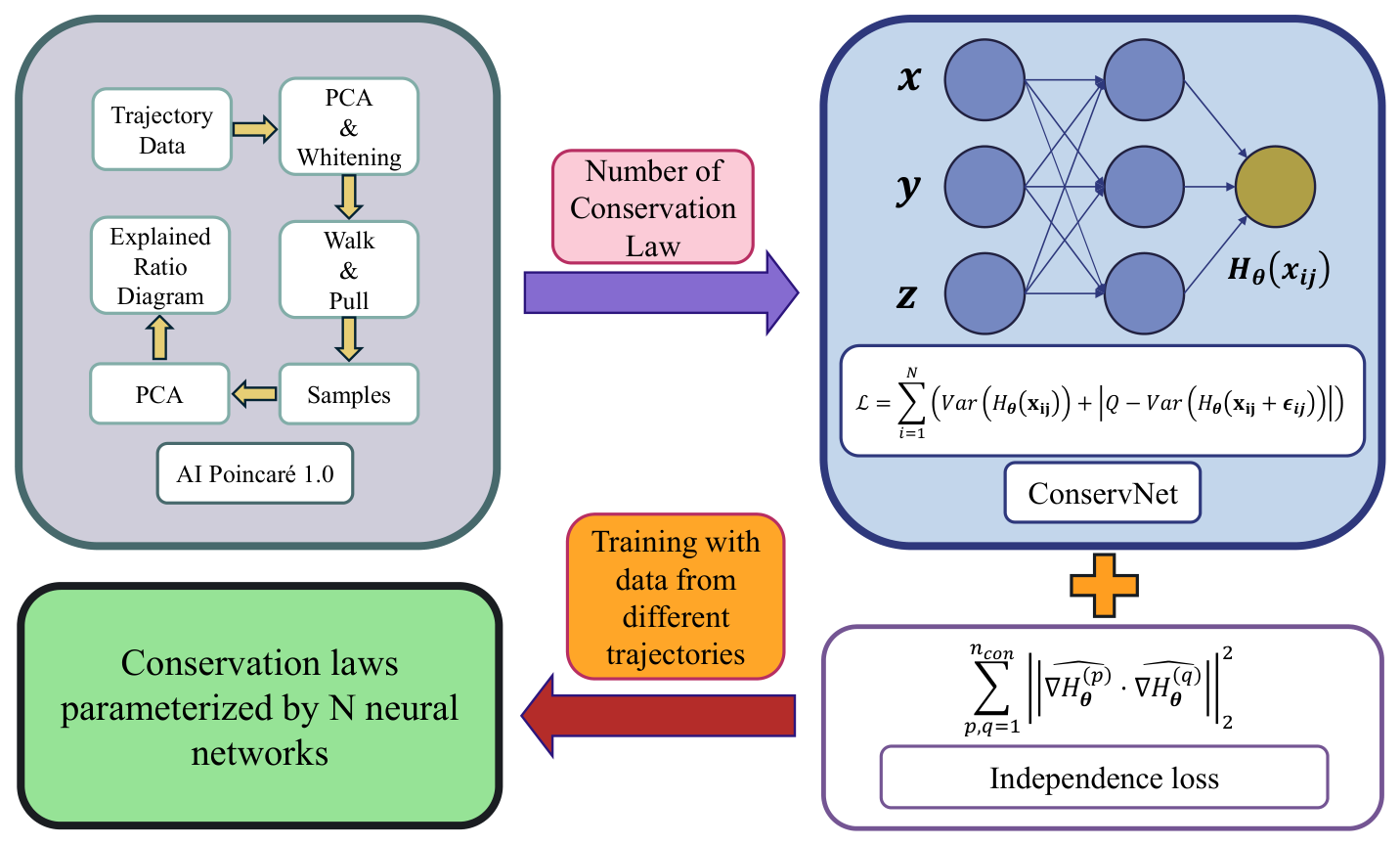
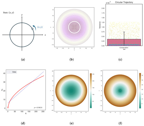
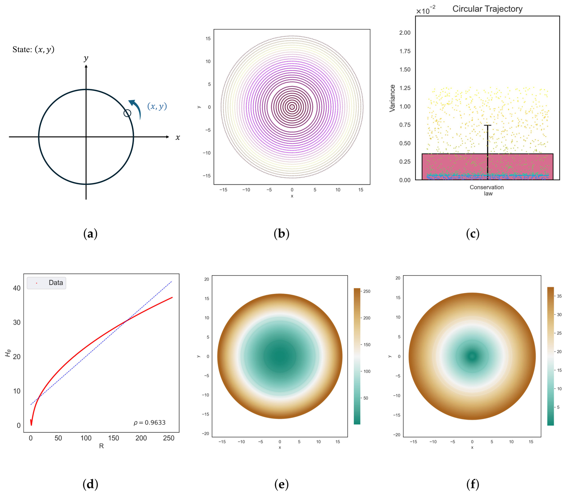
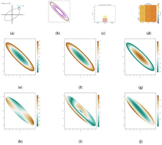
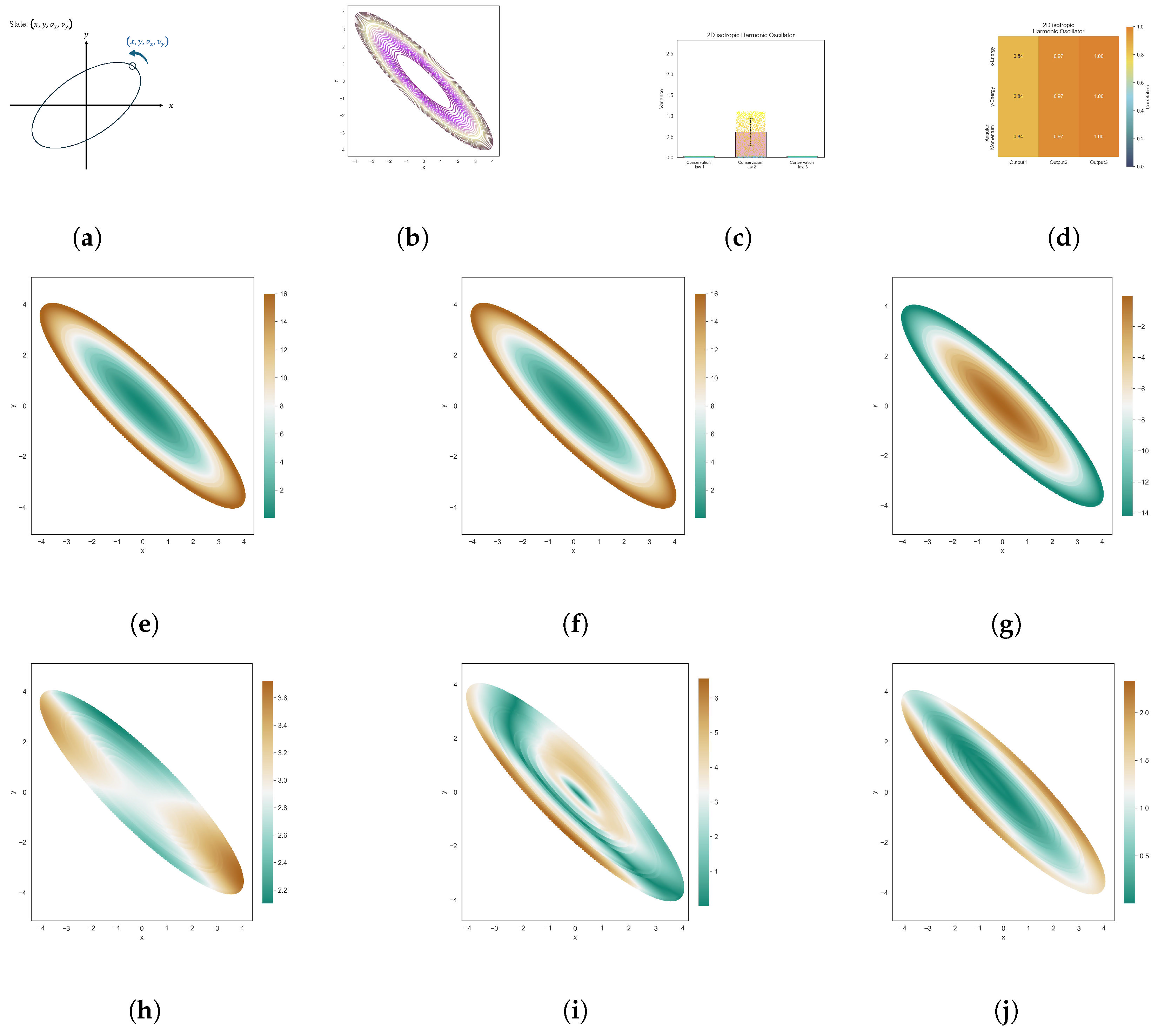
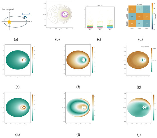
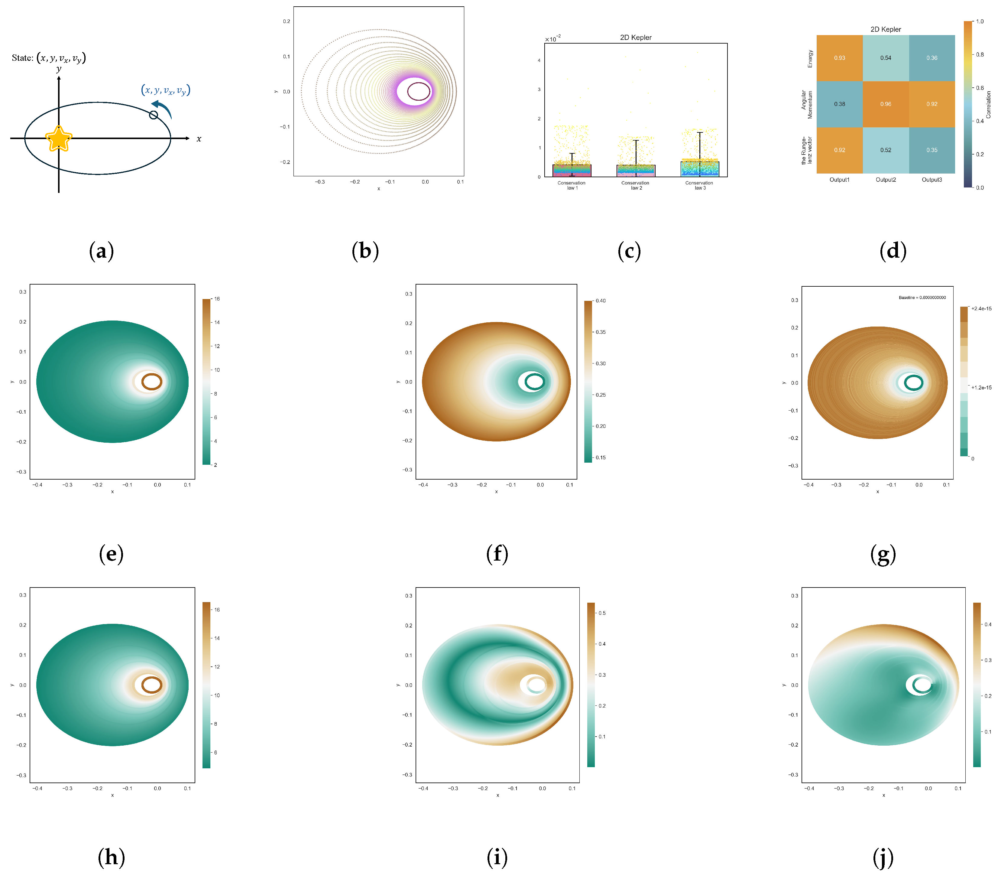
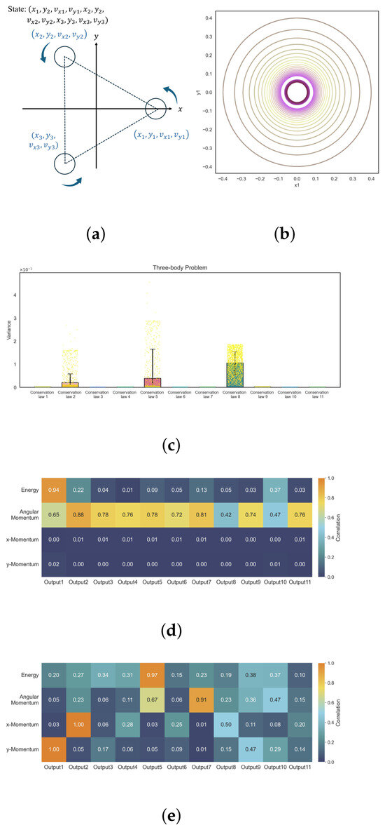
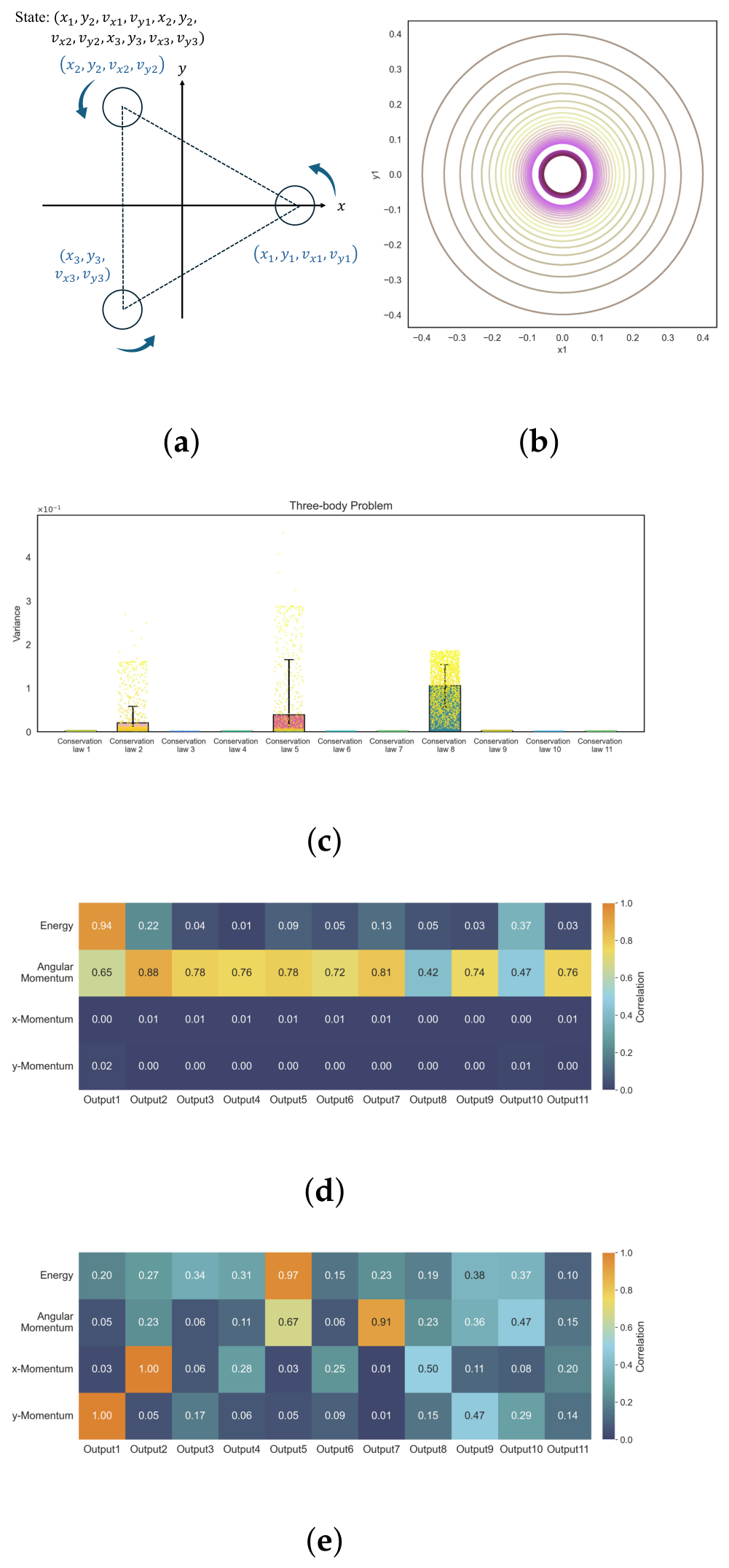
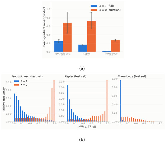
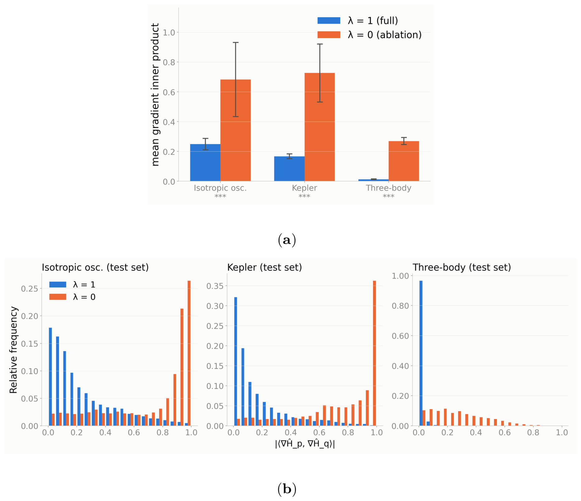
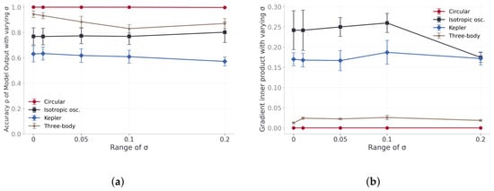
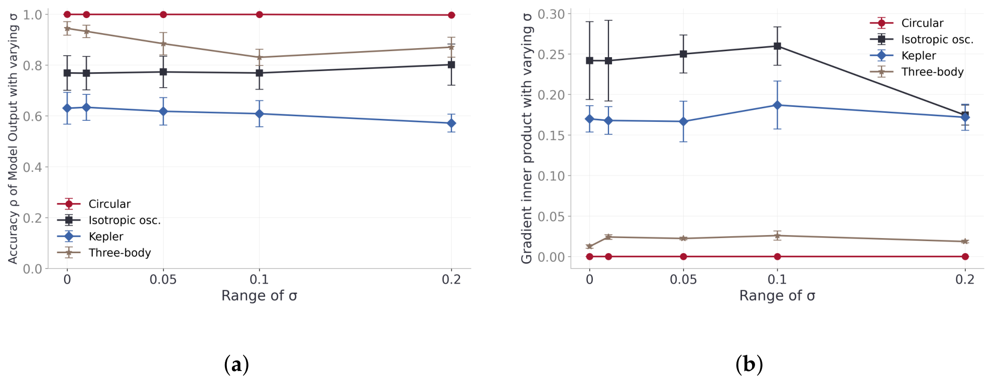
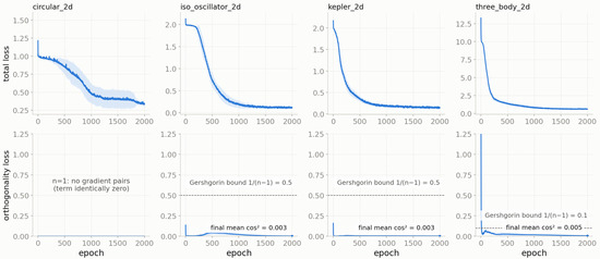
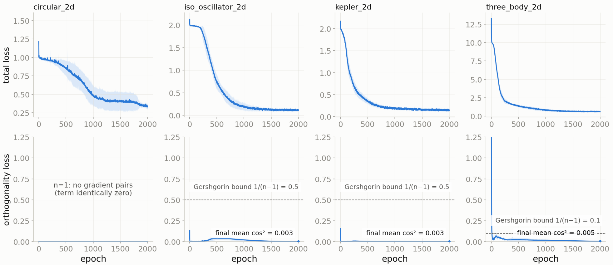
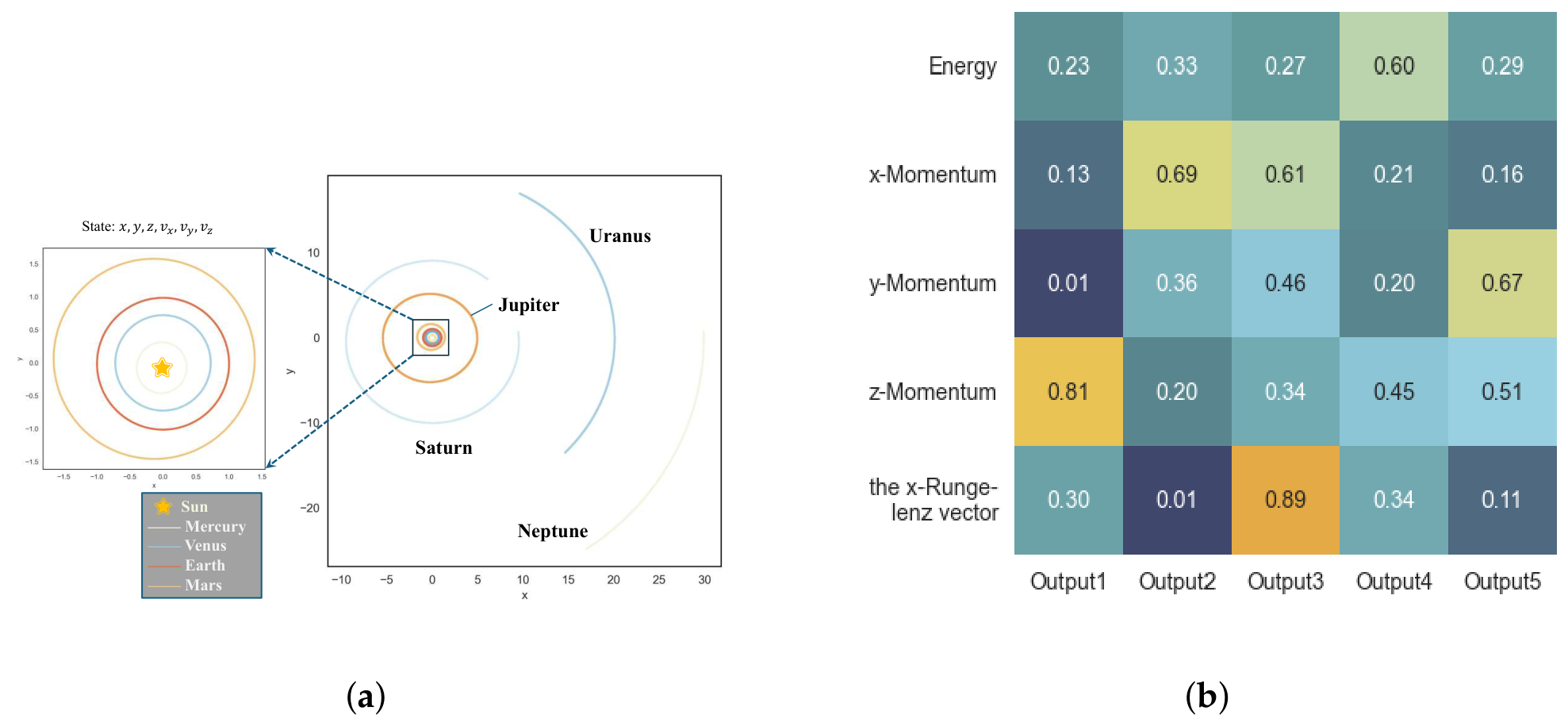

Disclaimer/Publisher’s Note: The statements, opinions and data contained in all publications are solely those of the individual author(s) and contributor(s) and not of MDPI and/or the editor(s). MDPI and/or the editor(s) disclaim responsibility for any injury to people or property resulting from any ideas, methods, instructions or products referred to in the content. |
© 2026 by the authors. Licensee MDPI, Basel, Switzerland. This article is an open access article distributed under the terms and conditions of the Creative Commons Attribution (CC BY) license.