Nonlinear Model Predictive Control for Tractors Based on an Efficient Neural Network Optimization Strategy

Abstract

The application and performance of Nonlinear Model Predictive Control (NMPC) are critically limited by the computational efficiency of solving nonlinear combinatorial optimization problems. To address this challenge, this study proposes an efficient optimization strategy that employs a neural network to solve the constrained L-1 norm minimization problem within the NMPC framework, thereby enhancing motion control performance. Inspired by the flexible representational capacity and powerful optimization capabilities of neural networks, we explicitly encode the NMPC objective function into a network architecture. The optimal control solution is then obtained efficiently through network training. We validate the proposed strategy in a tractor path-tracking control task, detailing the processes of network construction and optimization. Benefiting from the inherent parallelism and computational efficiency of neural networks, the resulting controller demonstrates excellent real-time performance. Specifically, with prediction horizons set to 5, 10, and 20 steps, the solution times are reduced to less than 0.12, 0.28, and 0.84 s, respectively, under typical operating constraints.

1. Introduction

The pursuit of unmanned farms has elevated the demands on tractor path-tracking control, increasingly requiring integration with dynamic obstacle avoidance and multi-vehicle cooperation. This evolution from automation to intelligence necessitates control strategies beyond traditional model-free approaches (e.g., PID) or simple geometric path following. Consequently, Model Predictive Control (MPC), with its inherent finite-horizon dynamic optimization capabilities, has emerged as a promising framework for achieving breakthroughs in intelligent tractor control.

While MPC has found widespread success in diverse fields such as industrial processes, robotics, and power electronics, its application to systems with inherent nonlinearities, like vehicle dynamics, faces a critical challenge. To ensure computational tractability, nonlinear models are often linearized, inevitably introducing prediction errors and potentially diminishing the controller’s performance advantage. This is particularly acute in motion control applications, such as tractor path-tracking, where stringent real-time requirements severely limit the direct application of Nonlinear MPC (NMPC). The core strength of MPC lies in its three pillars: (1) the use of a (potentially nonlinear) predictive model; (2) multi-step prediction; (3) online optimization to compute the control law. Yet, achieving high performance with NMPC demands a triad of conflicting requirements: an accurate nonlinear model, a sufficiently long prediction horizon for performance, and an extremely efficient optimization solver to meet real-time constraints—a combination that is often difficult to realize in practice.

1.1. Path Tracking Control Methods for Unmanned Tractors

Path tracking for agricultural vehicles is a well-established research area, with extensive work dedicated to various control methodologies. Classical PID-based controllers have been extensively explored, ranging from standard implementations [1] to those enhanced with genetic algorithms for parameter tuning [2]. To improve robustness, sliding mode control (SMC) strategies have been proposed, such as a dual-objective combined SMC for enhanced stability [3] and SMC for tractor-trailer systems under disturbance [4]. Fuzzy logic controllers, leveraging expert knowledge without requiring precise models, have also been applied to tractor control, demonstrating stable trajectory tracking [5] and human-like steering response [6]. More recently, Model Predictive Control (MPC) has gained traction for its ability to handle constraints systematically. Studies have shown its advantages, such as improved velocity and stability with relaxation factors [7] and superior handling of non-holonomic constraints compared to Linear Quadratic Regulators (LQR) [8]. While these methods, including MPC with linearized models, have shown promise, they often struggle to fully leverage complex nonlinear vehicle dynamics under real-time computation limits, motivating the exploration of more efficient nonlinear solution strategies.

1.2. Improving Efficiency of NMPC Optimization

Substantial research efforts have been dedicated to improving the computational efficiency of NMPC. The most prevalent approach involves avoiding direct nonlinear optimization by linearizing the nonlinear model under specific assumptions, thereby transforming the problem into a more tractable linear or quadratic program [9,10,11,12,13]. Another strategy focuses on reducing the frequency or complexity of online optimization. This includes event-triggered or self-triggered mechanisms that solve the optimization problem only when necessary [14,15,16,17,18], as well as adaptive techniques that narrow the search space or shorten the prediction horizon based on runtime conditions [19,20,21]. While effective for real-time implementation, these methods inherently compromise optimality or performance as they circumvent, rather than solve, the core nonlinear problem. A third category seeks to reformulate the problem into a more solvable form, often by employing duality or enforcing convexity under specific constraints [22,23]. However, such reformulations are typically problem-specific, may introduce complexity, and are not universally applicable.

1.3. Applications of Neural Networks to MPC

The remarkable success of Neural Networks (NNs) has inspired their integration into MPC frameworks, primarily in two ways. The first and most common is to use an NN as a function approximator for the MPC controller itself. Here, an offline-trained NN mimics the input–output mapping of a traditional NMPC solver, replacing the online optimization with a fast forward pass [24,25,26,27,28,29,30]. However, this method requires solving a vast number of optimization problems offline to generate training data, which itself can be prohibitive for complex problems. Furthermore, the resulting controller is fixed to specific horizon settings and may raise safety concerns due to generalization errors if the training data is insufficient [31].

The second approach employs NNs to learn an accurate predictive model of the system dynamics, which is then used within the MPC loop [32,33,34,35,36]. For instance, deep networks have been used to learn nonlinear state-space models [33], and Recurrent Neural Networks (RNNs) have been applied to predict state evolution [36]. A common theme in these studies is the use of local linear models or L2-norm cost functions, which, while effective, may not fully capture the desired control characteristics or exploit the potential of NNs for solving the optimization problem itself.

1.4. The Main Research of This Paper

The prevailing practice in NMPC, especially for applications with stringent real-time requirements like motion control, often resorts to model linearization to circumvent the computational intractability of direct nonlinear optimization. While practical, this approach inherently compromises accuracy and performance.

We take a fundamentally different perspective. Instead of viewing NNs merely as universal function approximators for controllers or models, we focus on the powerful optimization engines that underpin their training. The success of deep learning is built upon highly efficient, parallelizable optimization algorithms (e.g., backpropagation). We propose to leverage this very optimization infrastructure to solve the NMPC problem itself. Our core idea is to encode the NMPC problem—comprising the nonlinear model, constraints, and objective function—directly into the structure of an NN, transforming the optimal control problem into a network training task that can be solved rapidly using standard NN optimization tools.

The key distinctions and contributions of our work are:

Direct Problem Encoding, Not Approximation: We construct an NN that is a direct, one-to-one mathematical representation of the constrained L1-norm NMPC problem. This is not a black-box approximator trained on data but a white-box, interpretable computational graph where each component corresponds to a specific part of the optimization problem (dynamics, constraints, cost).

Exploiting NN Optimization Infrastructure: The solution is obtained by treating the current state and reference as inputs and performing a single, highly efficient forward/backward pass (training step) of this constructed network. This leverages the inherent parallelism and optimization efficiency of modern deep learning frameworks.

Advantages: This method avoids the offline data generation burden and safety concerns of approximation-based methods [31], as no pre-training on solved instances is required. It solves the exact problem online. Moreover, it is particularly well-suited for non-smooth L1-norm objectives, whose properties are preserved in the network formulation.

1.5. Chapter Organization and Math Notation

The remainder of this paper is organized as follows. Section 2 details the proposed control framework, including the tractor system model and the novel NN-based optimization strategy. Section 3 presents the specific application of this strategy to the tractor path-tracking problem. Section 4 provides experimental results and analysis. Finally, Section 5 concludes the paper and discusses future work.

The mathematical notation involved in this paper and its meaning are as follows: the m-dimensional set of vectors is denoted as ${\mathbb{R}}^m$. For vectors $\mathbf{a}$=$\left[\begin{array}{ccc}{a}_1& a_2& a_3\end{array}\right]$∈${\mathbb{R}}^3$, $\mathbf{b}$ = $\left[\begin{array}{ccc}{b}_1& b_2& b_3\end{array}\right]$∈${\mathbb{R}}^3$, $\left|\begin{array}{c}\mathbf{a}\end{array}\right|$ does not denote the modulus of the vector $\mathbf{a}$ but the sum of the absolute values of its elements $\left|\begin{array}{c}\mathbf{a}\end{array}\right|$=$\left|\begin{array}{c}{a}_1\end{array}\right|$+$\left|\begin{array}{c}{a}_2\end{array}\right|$+$\left|\begin{array}{c}{a}_3\end{array}\right|$, while ${\left|\begin{array}{c}\mathbf{a}\end{array}\right|}_{\mathbf{b}}$=$b_1\left|\begin{array}{c}{a}_1\end{array}\right|$+$b_2\left|\begin{array}{c}{a}_2\end{array}\right|$+$b_3\left|\begin{array}{c}{a}_3\end{array}\right|$, ${∥\begin{array}{c}\mathbf{a}\end{array}∥}_{\mathbf{Q}}^2$=${\mathbf{a}}^T\mathbf{Q}\mathbf{a}$. The expressions for the linear function (purelin), radial basis function (radbas), symmetric S-shaped function (tansig), positive linear function (poslin), positive-hard limiting function (hardlim), cosine function (cos), sinusoidal function (sin) and tangent function (tan) described in this paper are as follows: $purelin(x)=x$, $radbas(x)=exp(-x^2)$, $tansig(x)={\displaystyle \frac{2}{1+e^{-2x}}}$, ${\displaystyle poslin(x)=\left\{\begin{array}{c}x,x>0\hfill \\ 0,x\le 0\hfill \end{array}\right.}$, $cos(x)=cos(x)$, $sin(x)=sin(x)$, $tan(x)=tan(x)$.

2. Problem Description and Optimization Strategy

Assume that the system behavior can be described by a discrete nonlinear function (1):

$${\mathbf{x}}_{k+1}=f({\mathbf{x}}_k,{\mathbf{u}}_k)$$

(1)

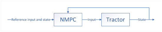
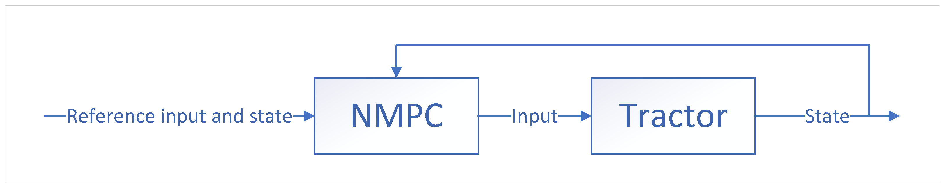
where ${\mathbf{x}}_k\in {\mathbb{R}}^d$ is the system state and ${\mathbf{u}}_k\in {\mathbb{R}}^m$ is input to the system at time k. For simplicity, system disturbances are not considered in this formulation. The proposed optimization strategy is implemented within an NMPC framework whose control block diagram is shown in Figure 1.

Figure 1. A block diagram of the proposed NMPC framework with the NN-based optimizer.

2.1. Objective Function

Generally, in order to drive the state sequence of the system as close as possible to the reference sequence at time k, the control increment sequence of NMPC can be obtained by solving objective function (2):

$$\mathbf{J}(k)=\underset{\Delta \mathbf{u}}{min}\left\{{\displaystyle \sum _{i=1}^{N_p}}\parallel \mathbf{x}(k+i|k)-{\mathbf{x}}_{\mathrm{ref}}{(k+i|k)\parallel }_{\mathbf{Q}}^2+{\displaystyle \sum _{i=1}^{N_c}}{\parallel \Delta \mathbf{u}(k+i-1|k)\parallel }_{\mathbf{R}}^2\right\}$$

(2a)

subject to:

$${\mathbf{x}}_{k+1}=f({\mathbf{x}}_k,{\mathbf{u}}_k)$$

(2b)

$${\mathbf{x}}_k={\mathbf{x}}_{\mathbf{0}},{\mathbf{u}}_{k-1}={\mathbf{u}}_{\mathbf{0}}$$

(2c)

$${\mathbf{u}}_k\in \mathcal{U},{\mathbf{x}}_k\in \mathcal{X},▵{\mathbf{u}}_k\in \mathcal{V}$$

(2d)

where $▵\mathbf{u}$ is input increment, which is also optimization variable, $\mathbf{u}(k+i-1|k)=\mathbf{u}(k+i-2|k)+▵\mathbf{u}(k+i-1|k),i=1,2,\dots ,N_c$; $\mathbf{u}(k+i-1|k)=\mathbf{u}(k+i-2|k),i=N_c+1,N_c+2,\dots ,N_p$; $N_p$ and $N_c$ are predictive horizon and control horizon, respectively, and $N_p\ge N_c$, matrices $\mathbf{Q}$ and $\mathbf{R}$ are weight matrices of state and control increment penalty, respectively. ${\mathbf{x}}_{ref}(k+1|k)$ is the reference state at time k for the system at time $k+i$, ${\mathbf{x}}_0$ and ${\mathbf{u}}_0$ are the state at time k and the input at time $k-1$, respectively. $\mathcal{U},\mathcal{X},\mathcal{V}$ are constraint sets for input ${\mathbf{u}}_k$, state ${\mathbf{x}}_k$ and input increment $▵{\mathbf{u}}_k$, respectively. The purpose of the first term in objective function (2) is mainly to drive the state sequence of the system close to the reference sequence, while the second term is to make the input to the system (i.e., the control output of the controller) vary as little as possible.

2.2. Optimization Strategy Based on Recursive Neural Network

To facilitate its embedding into a neural network structure, we reformulate the objective function using the L1-norm, which is naturally compatible with certain activation functions. We consider the following modified objective function (3):

$$\begin{array}{cc}\hfill \mathbf{J}(k)& =\underset{▵\mathbf{u}}{min}\{{\displaystyle \sum _{i=1}^{N_p}}{|\mathbf{u}(k+i-1|k)-{\mathbf{u}}_{ref}(k+i-1|k)|}_{\mathbf{p}(i)}\hfill \\ \hfill & +{\displaystyle \sum _{i=1}^{N_p}}{|\mathbf{x}(k+i|k)-{\mathbf{x}}_{ref}(k+i|k)|}_{\mathbf{q}(i)}\hfill \\ \hfill & +{\displaystyle \sum _{i=1}^{N_c}}{|▵\mathbf{u}(k+i-1|k)|}_{\mathbf{r}(i)}\}\hfill \end{array}$$

(3a)

subject to:

$${\mathbf{x}}_{k+1}=f({\mathbf{x}}_k,{\mathbf{u}}_k)$$

(3b)

$${\mathbf{x}}_k={\mathbf{x}}_0,{\mathbf{u}}_{k-1}={\mathbf{u}}_0$$

(3c)

$${\mathbf{u}}_k\in \mathcal{U},{\mathbf{x}}_k\in \mathcal{X},▵{\mathbf{u}}_k\in \mathcal{V}$$

(3d)

where ${\mathbf{u}}_{ref}(k+i|k),i=1,2,\dots ,N_p$ is the reference input at time k for the system at time $k+i$. $\mathbf{p}(i)$, $\mathbf{q}(i)$ and $\mathbf{r}(i)$ are penalty weights of input, state and input increment, respectively. Other symbols have the same meanings as objective function (2).

The inclusion of the input reference term $|\mathbf{u}-{\mathbf{u}}_{ref}|$ serves two purposes: (1) In many systems (e.g., our tractor case study), control inputs like velocity and steering angle are also critical states that require tracking. (2) It allows the incorporation of prior knowledge (e.g., a geometric reference for steering angle, $\delta \approx arctan(L/R)$, where L is the wheelbase and R the turning radius) to guide the controller, potentially improving performance.

Directly handling hard constraints within the neural network optimization framework is challenging due to its reliance on gradient-based global search. Therefore, following common practice in MPC [37,38,39,40,41], we convert the hard constraints (3d) into soft constraints via penalty functions. This transforms problem (3) into an unconstrained (but penalized) optimization problem (4):

$$\begin{array}{cc}\hfill \mathbf{J}(k)& =\underset{▵\mathbf{u}}{min}\{{\displaystyle \sum _{i=1}^{N_p}}{|\mathbf{u}(k+i-1|k)-{\mathbf{u}}_{ref}(k+i-1|k)|}_{\mathbf{p}(i)}\hfill \\ \hfill & +{\displaystyle \sum _{i=1}^{N_p}}{|\mathbf{x}(k+i|k)-{\mathbf{x}}_{ref}(k+i|k)|}_{\mathbf{q}(i)}\hfill \\ \hfill & +{\displaystyle \sum _{i=1}^{N_c}}{|▵\mathbf{u}(k+i-1|k)|}_{\mathbf{r}(i)}\hfill \\ \hfill & +M_1{\displaystyle \sum _{i=1}^{N_p}}penalty1(\mathbf{u}(k+i-1|k))\hfill \\ \hfill & +M_2{\displaystyle \sum _{i=1}^{N_p}}penalty2(\mathbf{x}(k+i|k))\hfill \\ \hfill & +M_3{\displaystyle \sum _{i=1}^{N_c}}penalty3(▵\mathbf{u}(k+i-1|k))\}\hfill \end{array}$$

(4a)

subject to:

$${\mathbf{x}}_{k+1}=f({\mathbf{x}}_k,{\mathbf{u}}_k)$$

(4b)

$${\mathbf{x}}_k={\mathbf{x}}_0,{\mathbf{u}}_{k-1}={\mathbf{u}}_0$$

(4c)

where ${\displaystyle penalty1(\mathbf{u})=\left\{\begin{array}{c}g(\mathbf{u}),\mathbf{u}\notin \mathcal{U}\hfill \\ 0,\mathbf{u}\in \mathcal{U}\hfill \end{array}\right.}$, ${\displaystyle penalty2(\mathbf{x})=\left\{\begin{array}{c}h(\mathbf{x}),\mathbf{x}\notin \mathcal{X}\hfill \\ 0,\mathbf{x}\in \mathcal{X}\hfill \end{array}\right.}$, ${\displaystyle penalty3(▵\mathbf{u})=\left\{\begin{array}{c}i(▵\mathbf{u}),▵\mathbf{u}\notin \mathcal{V}\hfill \\ 0,▵\mathbf{u}\in \mathcal{V}\hfill \end{array}\right.}$, $g(\mathbf{u})>0,h(\mathbf{x})>0,i(▵\mathbf{u})>0$ are called penalty functions. $M_1$, $M_2$ and $M_3$ are constant weights. For objective function (4), in order to minimize violations of those penalty functions, $M_1$, $M_2$ and $M_3$ should be large enough. And related results are discussed in detail in articles [39,41]. Other symbols have the same meanings as objective function (3).

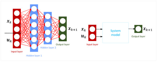
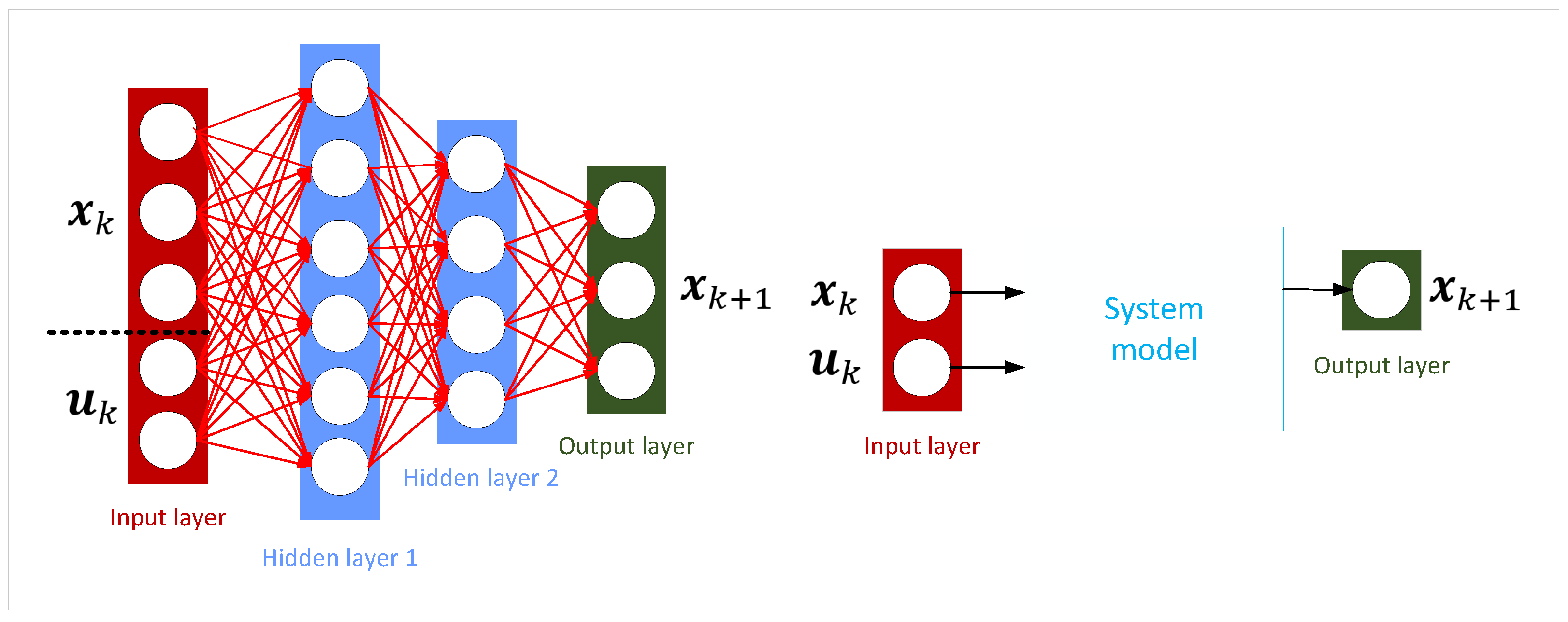
Core Idea: Encoding the Optimization Problem as a Neural Network. The central concept of our strategy is to construct a neural network that is mathematically equivalent to the optimization problem (4). This network is not a black-box approximator but a white-box, interpretable computational graph whose forward pass computes the objective function value $J(k)$, and whose trainable weights correspond to the optimization variables $▵\mathbf{u}$. Constructing the System Model Sub-network. The dynamical model (1) must first be represented as a network module. While a sub-network could be trained to approximate $f(·)$ from data—a method compatible with data-driven approaches—this may introduce approximation errors that accumulate over the prediction horizon. For high-fidelity control, we recommend constructing an interpretable, physics-inspired network that exactly encodes the known model $f(·)$ using appropriate, differentiable activation functions (e.g., tan, sin, cos for kinematic relations). This ensures no loss of model accuracy. The construction of such a model network for a tractor is detailed in Section 3. Figure 2 shows a schematic of a generic system model network, where black connections have a fixed weight of 1.

Figure 2. Neural network module representing the system dynamics $f({\mathbf{x}}_k,{\mathbf{u}}_k)$.

Penalty Term Networks. Each component of the objective function (4a) is likewise constructed as a simple interpretable network module.

• Control Effort Penalty: The term ${|▵\mathbf{u}|}_{\mathbf{r}(i)}$ is implemented by the network shown in Figure 3. It consists of linear (purelin) activation neurons. The input layer (pink) receives $▵\mathbf{u}$, which is multiplied by the weight $r(i)$ (sky-blue connection) to produce the penalty output (green). Black connections have a weight of 1.
• Input Reference Penalty: The term $|\mathbf{u}-{\mathbf{u}}_{ref}{|}_{\mathbf{p}(i)}$ is constructed similarly, as shown in Figure 4. It computes the difference between u and ${\mathbf{u}}_{ref}$ before applying the weight $\mathbf{p}(i)$.
• State Reference Penalty: The term $|\mathbf{x}-{\mathbf{x}}_{ref}{|}_{\mathbf{q}(i)}$ is implemented analogously (Figure 5).
• Constraint Penalty: The soft constraint penalty $M_2·penalty2(\mathbf{x})$ is implemented by the network in Figure 6. The key element is a neuron (purple) whose activation function is the piecewise-defined penalty function itself. Similar networks are constructed for input and input increment constraints.

Figure 3. Network module for the control effort penalty term ${|▵\mathbf{u}|}_{\mathbf{r}}$.

Figure 3. Network module for the control effort penalty term ${|▵\mathbf{u}|}_{\mathbf{r}}$.

Figure 4. Network module for the input reference tracking penalty term ${|\mathbf{u}-{\mathbf{u}}_{\mathrm{ref}}|}_{\mathbf{p}}$.

Figure 4. Network module for the input reference tracking penalty term ${|\mathbf{u}-{\mathbf{u}}_{\mathrm{ref}}|}_{\mathbf{p}}$.

Figure 5. Network module for the state reference tracking penalty term ${|\mathbf{x}-{\mathbf{x}}_{\mathrm{ref}}|}_{\mathbf{q}}$.

Figure 5. Network module for the state reference tracking penalty term ${|\mathbf{x}-{\mathbf{x}}_{\mathrm{ref}}|}_{\mathbf{q}}$.

Figure 6. Network module for the state constraint penalty term $M_2·{\mathrm{penalty}}_{\mathcal{X}}(\mathbf{x})$.

Figure 6. Network module for the state constraint penalty term $M_2·{\mathrm{penalty}}_{\mathcal{X}}(\mathbf{x})$.

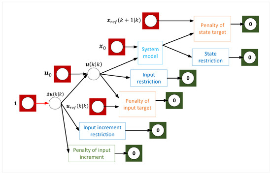
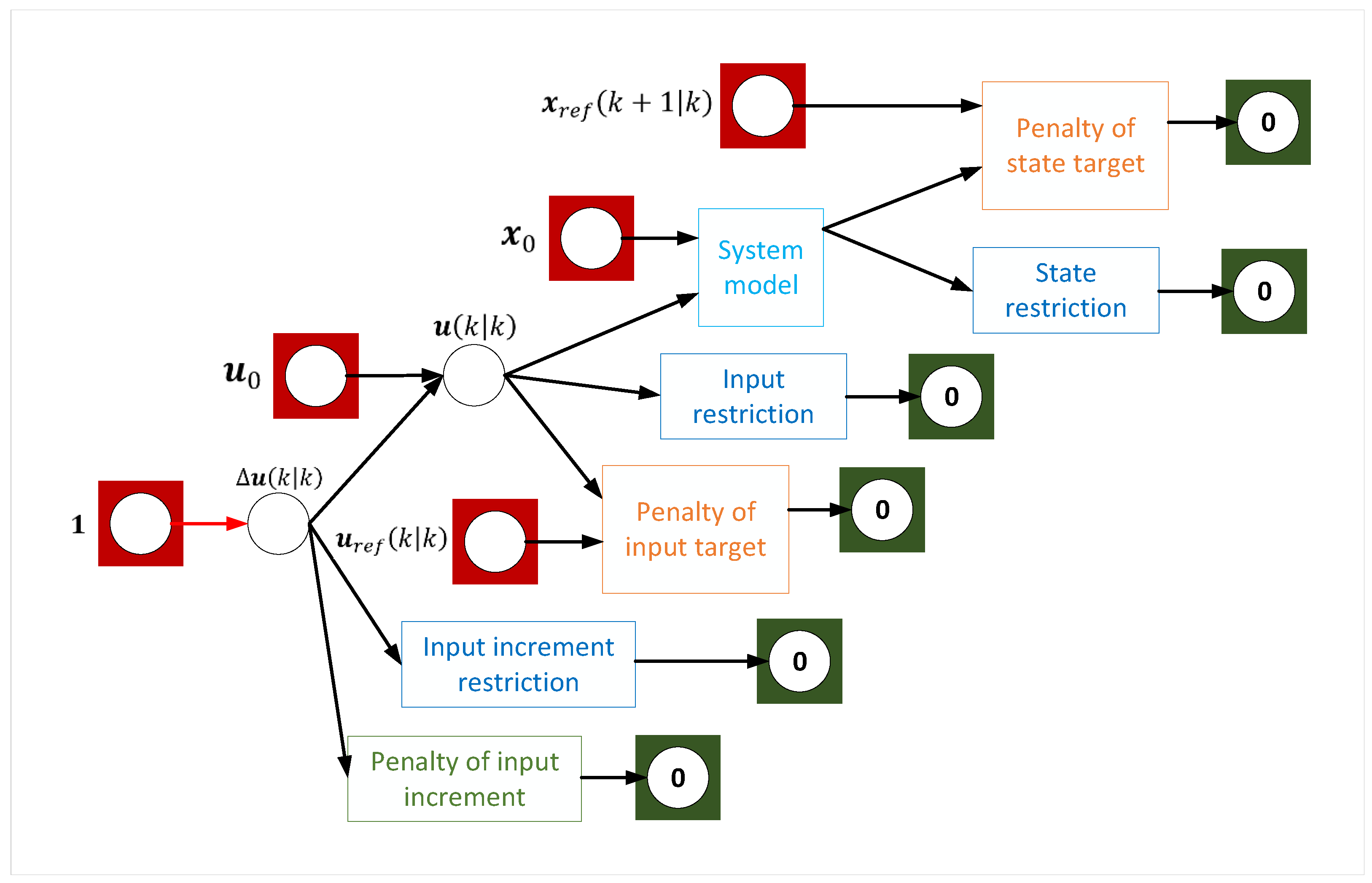
Complete Network for a Single-Step Horizon ($N_c=N_p=1$). These modular networks are combined to form the complete computational graph representing the entire objective function $\mathbf{J}(k)$. Figure 7 illustrates this for the simple case of $N_c=N_p=1$. The input layer (pink) receives all known parameters: a bias unit (1), the initial state ${\mathbf{x}}_0$, the previous input ${\mathbf{u}}_0$, and the reference signals ${\mathbf{u}}_{ref}(k|k)$ and ${\mathbf{u}}_{ref}(k+1|k)$. The output layer (green) has a single neuron whose target value is set to 0, corresponding to the minimization of $\mathbf{J}(k)$. All internal neurons use linear (purelin) activations. Crucially, the red connections represent the trainable weights, which correspond exactly to the optimization variables $▵\mathbf{u}(k|k)$.

Figure 7. Complete neural network for the simplified NMPC problem ($N_c=N_p=1$).

Solving the Optimization via Network Training. The optimization problem is solved by training this constructed network. Standard backpropagation and gradient-based optimizers (e.g., Adam, SGD) are applied to adjust only the red weights (the control increments $▵\mathbf{u}$) to minimize the network’s output (the objective function $\mathbf{J}(k)$. Upon convergence, the final values of these red weights are the optimal solution $▵{\mathbf{u}}^{*}(k|k)$. This approach transforms a constrained nonlinear optimization into a standard neural network training task, leveraging highly efficient, parallelizable, and robust off-the-shelf optimization algorithms.

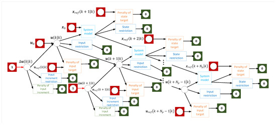
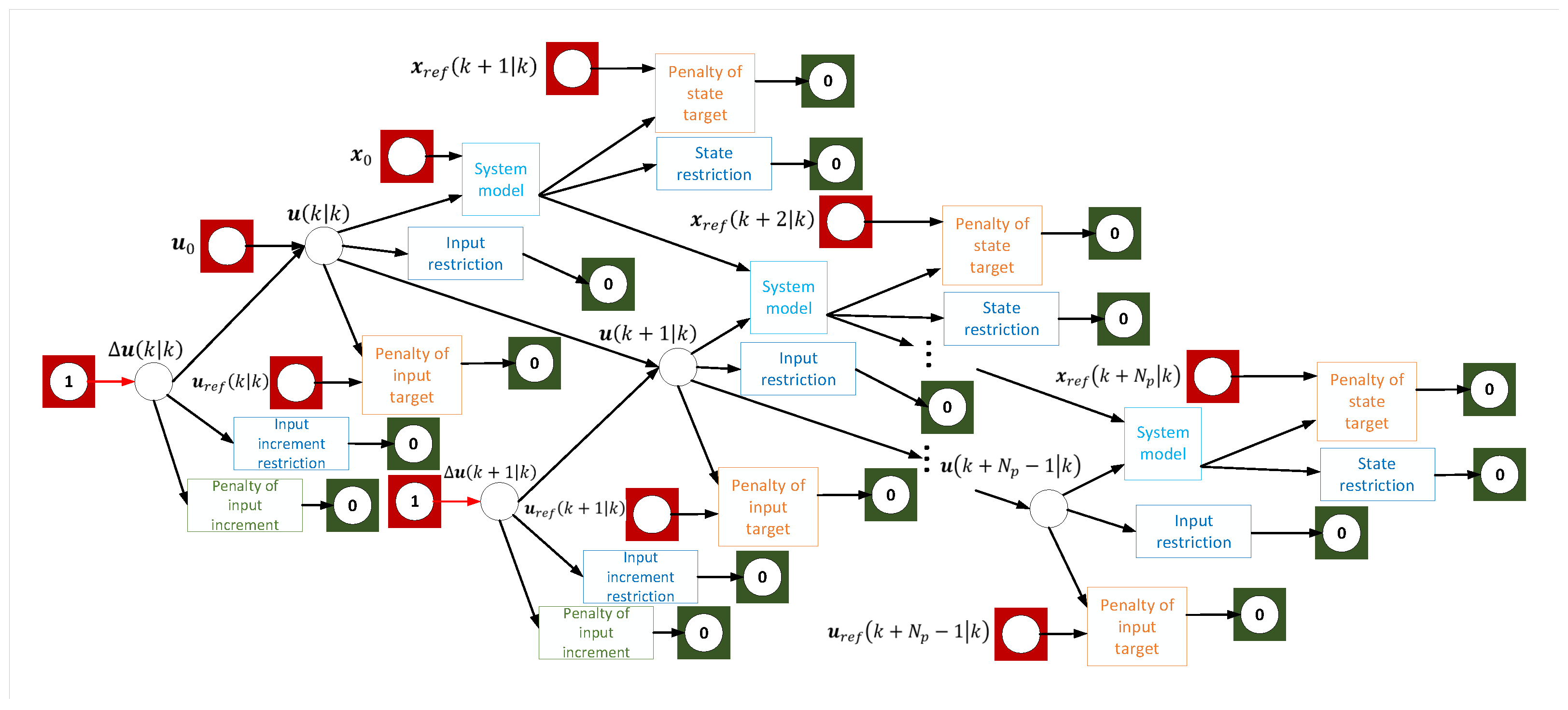
General Case: Multi-Step Horizon and Recursive Structure. For the general case of $N_c\ne N_p$, the network adopts a recursive structure as shown in Figure 8. This structure efficiently unrolls the prediction dynamics over time, reusing the same system model sub-network at each step. This recursion is not only a compact representation but also leverages the efficiency of backpropagation through time (BPTT), where gradient information can be stored and reused, leading to fast solution times—a critical advantage for multi-step NMPC problems. The interpretation of input/output layers and connection weights remains the same as in the single-step case. Training this recursive network yields the optimal control sequence $\{▵{\mathbf{u}}^{*}(k|k),\dots ,▵{\mathbf{u}}^{*}(k+N_c-1|k)\}$.

Figure 8. Recursive neural network architecture for the complete NMPC problem with $N_p>N_c\ge 1$. Trainable weights (red) correspond to the control sequence $▵\mathbf{u}$.

3. Application to Tractor Path-Tracking Control

This section details the application of the proposed neural network-based optimization strategy to the path-tracking control of an autonomous tractor, serving as a concrete case study.

3.1. Kinematic Model and Its Neural Network Construction

When vehicle kinematic model (5) is utilized as the system model:

$$\begin{array}{cc}\hfill & x_{k+i}=cos{\phi }_k\times v_{k}T+x_k\hfill \\ \hfill & y_{k+i}=sin{\phi }_k\times v_{k}T+y_k\hfill \\ \hfill & {\phi }_{k+i}={\displaystyle \frac{tan{\delta }_k}{l}}\times v_{k}T+{\phi }_k\hfill \end{array}$$

(5)

where the state vector is ${\mathbf{x}}_k={[x_k,y_k,{\phi }_k]}^T$, representing the tractor’s 2D position and heading angle. The control input vector is ${\mathbf{u}}_k={[v_k,{\delta }_k]}^T$,representing its velocity and steering angle. The parameters T (sampling period) and l (wheelbase) are constants.

The steering angle referred to in this study is derived from the kinematic model. Given that model-based control inherently possesses a certain degree of robustness, it is neither necessary nor practically feasible to ensure that the steering angle commanded by the controller always matches the actual steering angle of the tires. In fact, the controller is capable of compensating for such discrepancies through the mechanisms of receding-horizon optimization and feedback correction.

To embed this known model exactly into the optimization framework, we construct a white-box neural network that computes Equation (5). This requires implementing basic arithmetic operations, notably multiplication, within the network.

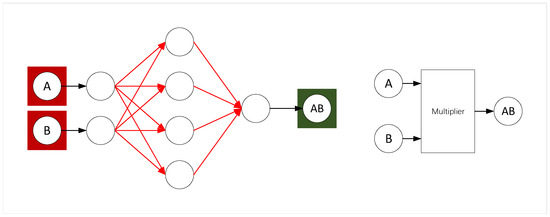
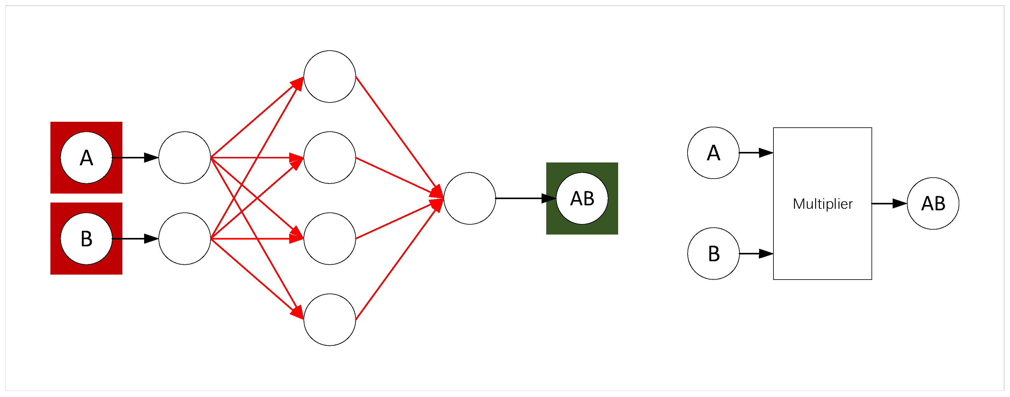
Multiplication Module: Following the analytic method of Lin et al. [10], we construct a minimal, high-precision multiplier network rather than training one. Figure 9 shows this two-layer network. It takes two inputs (pink) and produces their product as output (green). The hidden layer uses neurons with a non-linear activation function with a non-zero second-order derivative at zero (e.g., radbas), while the output neuron uses a linear (purelin) activation. All weights (black) are fixed to 1 or other specific analytic values as derived in [10], making this module an exact, parameter-free computational block.

Figure 9. Analytically constructed neural network module for exact multiplication.

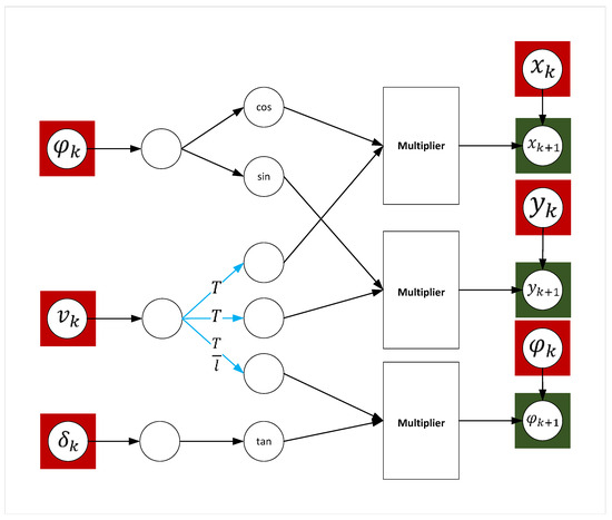
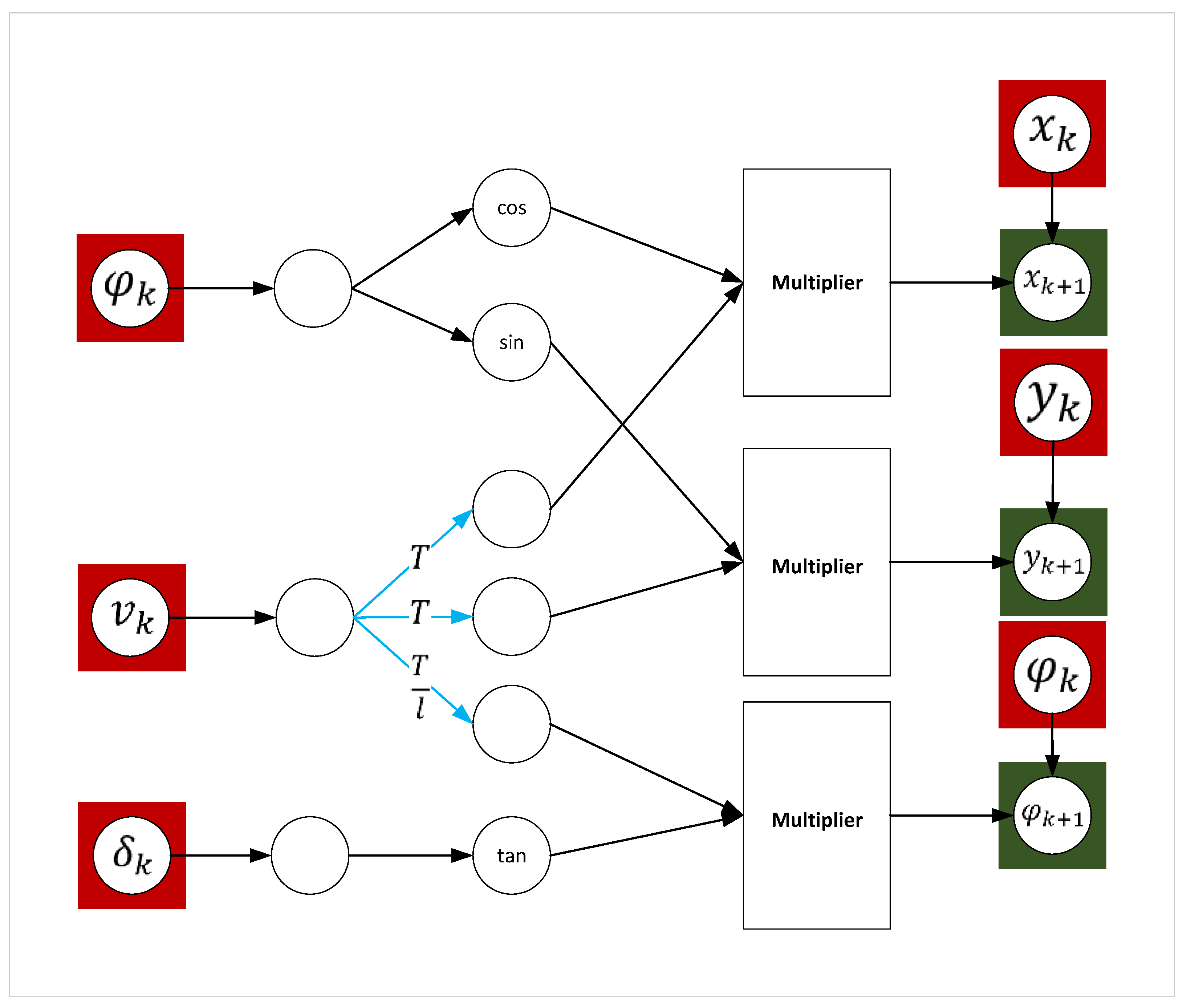
Complete Model Network: Using the multiplier module, along with neurons implementing trigonometric (sin, cos, tan) and linear (purelin) functions, we assemble the complete system model network shown in Figure 10. This network is a direct, interpretable translation of Equation (5): given the current state ${[x_k,y_k,{\phi }_k]}^T$, and input ${[v_k,{\delta }_k]}^T$ (pink input layer), its output (green) is precisely the next state ${[x_{k+1},y_{k+1},{\phi }_{k+1}]}^T$ calculated by the kinematic model.

Figure 10. Interpretable neural network encoding the tractor kinematic model (Equation (5)).

3.2. Neural Network Expression of Constraint Penalty Functions

We now detail the construction of the penalty function networks, concretizing the abstract penalty modules from Section 2.2 (e.g., Figure 6). For the tractor, we consider:

• Input Increment Constraints: $a\le ▵v_i\le b,c\le ▵{\delta }_i\le d$ for $i=1,2,\dots ,N_c$.
• Input Constraints: $A\le v_i\le B,C\le {\delta }_i\le D,$ for $i=1,2,\dots ,N_p$.
• State (Obstacle) Constraint: ${(x_i-o_x)}^2+{(y_i-o_y)}^2\ge r^2$ for $i=1,2,\dots ,N_p$, representing a circular obstacle at $(o_x,o_y)$ with radius r.

These hard constraints are converted into soft penalties. For example, the velocity constraint $A\le v\le B$ corresponds to the penalty function:

$${\mathrm{penalty}}_v(v)=max(A-v,0)+max(v-B,0).$$

(6)

This function outputs 0 when the constraint is satisfied and a positive value proportional to the violation otherwise. Similarly, the obstacle constraint is enforced by:

$${\mathrm{penalty}}_{\mathrm{obs}}(d)=max(E-d,0),$$

(7)

where $d={(x_i-o_x)}^2+{(y_i-o_y)}^2$ and $E=r^2$.

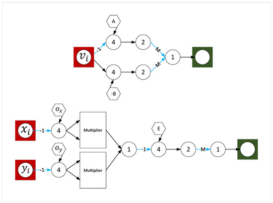
Figure 11 shows the network implementation of these two penalty functions, utilizing the positive linear (poslin, i.e., $max(·,0)$) activation function.

Figure 11. Neural network modules implementing the soft constraint penalty functions: (top) velocity bounds (Equation (6)); (bottom) circular obstacle avoidance (Equation (7)).

• Velocity Penalty Network (Top): Implements Equation (6). The input v is routed through two parallel branches computing $max(A-v,0)$ and $max(v-B,0)$, which are then summed.
• Obstacle Penalty Network (Bottom): Implements Equation (7). It first computes the squared distance d using multiplier modules, then applies $max(E-d,0)$.

Networks for other box constraints $(\delta ,▵v,▵\delta )$ are constructed analogously. The scalar weight M attached to the output (green) corresponds to the large penalty weight $M_1,M_2,M_3$ in Equation (4a).

3.3. Integrated Objective Function for Path-Tracking

The complete NMPC optimization problem for tractor path-tracking is formulated by integrating the constructed modules into the recursive network architecture of Figure 7. The resulting objective function is:

$$\begin{array}{cc}\hfill \mathbf{J}(k)& =\underset{▵v,▵\delta }{min}\{{\displaystyle \sum _{i=1}^{N_p}}{|v(k+i-1|k)-v_{ref}(k+i-1|k)|}_{p_1(i)}\hfill \\ \hfill & +{\displaystyle \sum _{i=1}^{N_p}}{|\delta (k+i-1|k)-{\delta }_{ref}(k+i-1|k)|}_{p_2(i)}\hfill \\ \hfill & +{\displaystyle \sum _{i=1}^{N_p}}{|x(k+i|k)-x_{ref}(k+i|k)|}_{q_1(i)}\hfill \\ \hfill & +{\displaystyle \sum _{i=1}^{N_p}}{|y(k+i|k)-y_{ref}(k+i|k)|}_{q_2(i)}\hfill \\ \hfill & +{\displaystyle \sum _{i=1}^{N_p}}{|\phi (k+i|k)-{\phi }_{ref}(k+i|k)|}_{q_3(i)}\hfill \\ \hfill & +{\displaystyle \sum _{i=1}^{N_c}}{|▵v(k+i-1|k)|}_{r_1(i)}\hfill \\ \hfill & +{\displaystyle \sum _{i=1}^{N_c}}{|▵\delta (k+i-1|k)|}_{r_2(i)}\hfill \\ \hfill & +M{\displaystyle \sum _{i=1}^{N_p}}penalty(v(k+i-1|k))\hfill \\ \hfill & +M{\displaystyle \sum _{i=1}^{N_p}}penalty(\delta (k+i-1|k))\hfill \\ \hfill & +M{\displaystyle \sum _{i=1}^{N_p}}penalty(distance(k+i|k))\hfill \\ \hfill & +M{\displaystyle \sum _{i=1}^{N_c}}penalty(▵v(k+i-1|k))\hfill \\ \hfill & +M{\displaystyle \sum _{i=1}^{N_c}}penalty(▵\delta (k+i-1|k))\}\hfill \end{array}$$

(8a)

subject to:

$$\left[\begin{array}{c}{x}_{k+1}\\ y_{k+1}\\ {\phi }_{k+1}\end{array}\right]=f(\left[\begin{array}{c}{x}_k\\ y_k\\ {\phi }_k\end{array}\right],\left[\begin{array}{c}{v}_k\\ {\delta }_k\end{array}\right])$$

(8b)

$$\left[\begin{array}{c}{x}_k\\ y_k\\ {\phi }_k\end{array}\right]=\left[\begin{array}{c}{x}_0\\ y_0\\ {\phi }_0\end{array}\right],\left[\begin{array}{c}{v}_{k-1}\\ {\delta }_{k-1}\end{array}\right]=\left[\begin{array}{c}{v}_0\\ {\delta }_0\end{array}\right]$$

(8c)

where $▵v,▵\delta$ are input increments of the velocity and steering angle of the tractor, and they are also optimization variables. $v(k+i-1|k)=v(k+i-2|k)+▵v(k+i-1|k),i=1,2,\dots ,N_c$; $v(k+i-1|k)=v(k+i-2|k),i=N_c+1,N_c+2,\dots ,N_p$; $\delta (k+i-1|k)=\delta (k+i-2|k)+▵\delta (k+i-1|k),i=1,2,\dots ,N_c$; $\delta (k+i-1|k)=\delta (k+i-2|k),i=N_c+1,N_c+2,\dots ,N_p$. $N_p$ and $N_c$ are the predictive horizon and the control horizon, respectively, and $N_p\ge N_c$. $q,p$ and r are penalty weights associated with state, input and input increment, respectively. $x_{ref}(k+i|k),y_{ref}(k+i|k)$ and ${\phi }_{ref}(k+i|k)$ are reference of x, y-coordinate and heading angle at time $k+i$, respectively, for the tractor at time k. f is the vehicle kinematic model (5) described in this section. ${\left[x_0{y}_0{\phi }_0\right]}^T$ and ${\left[v_0{\delta }_0\right]}^T$ are the state at time k and the input of the tractor at time $k-1$, respectively.

Item 1 and 2 of objective function (8) are to drive velocity and steering angle of tractor as close as possible to given reference, item 3, 4 and 5 are to drive trajectory and heading of tractor track reference path and direction, and item 6 and 7 are to hope that input increment of tractor is as close as possible to 0, that is, control output of controller changes as little as possible, and control can be more smooth.

4. Experimental Results and Analysis

This section presents a comprehensive experimental evaluation of the proposed neural network-based optimization strategy for tractor path-tracking. The experiments are designed to validate the algorithm’s computational efficiency, control performance (including path-tracking and obstacle avoidance), and its advantages over conventional methods. All simulations were conducted on a PC with an Intel i5-10400 CPU (2.90 GHz) and 16 GB RAM, running Windows 10. The controller was implemented in MATLAB (R2020a)/Simulink, while the high-fidelity vehicle dynamics were simulated using CarSim [42], a widely recognized platform in vehicle dynamics research. The system setup is summarized in Table 1. Carsim provides a powershift gearbox, and the driving power comes from a rear-wheel-drive electric motor. The basic parameters of the tractor are as follows: sprung mass is 3000 kg, roll inertia is 377 $\mathrm{kg}·{\mathrm{m}}^2$, pitch inertia is 1765 $\mathrm{kg}·{\mathrm{m}}^2$, and yaw inertia is 1765 $\mathrm{kg}·{\mathrm{m}}^2$.

Table 1. Hardware and software specifications of the experimental platform.

Operating System	CPU Type	CPU Base Frequency
Window 10	i5-10400	2.90 GHz
Memory Capacity/Frequency	Hard Disk Type
16 GB/3000 MHz	Solid-State Drive

4.1. Controller Configuration and Experimental Scenarios

The controller’s core parameters are listed in Table 2. A prediction horizon ($N_p$) and control horizon ($N_c$) of 10 steps with a sampling period $T_s=0.1$ s were used. The weighting matrices in the cost function (8a) were tuned to balance tracking accuracy and control smoothness. Physical constraints for the tractor’s velocity (v), steering angle ($\delta$), and their increments $(▵v,▵\delta )$ were enforced. A circular obstacle with a radius of 0.5 m was placed at coordinates (10, 0), with a large penalty weight $M=999$ to approximate a hard constraint. The reference path consisted of straight segments and arcs with a turning radius of 5 m, accompanied by corresponding velocity and steering angle references.

Table 2. Parameter configuration for the path-tracking controller.

Predictive horizon	Control horizon	Control period	Weight of velocity increment	Weight of velocity target
10	10	0.1 s	0.1	0.4
Weight of steering angle increment	Weight of steering angle target	Weight of position	Weight of heading angle	Constraint constant M
0.7	0.1	1	0.1	999,999
Lower bound of constraint of velocity increment	Upper bound of constraint of velocity increment	Lower bound of constraint of velocity	Upper bound of constraint of velocity	Lower bound of constraint of steering angle increment
−0.5 m/s	0.5 m/s	0 m/s	5 m/s	−1 rad
Upper bound of constraint of steering angle increment	Lower bound of constraint of steering angle	Upper bound of constraint of steering angle	Location of obstacle	Radiu of obstacle
1 rad	−1.1 rad	1.1 rad	[10, 0]	0.5 m
Reference velocity of straight forward	Reference velocity of turning	Reference steering angle of straight forward	Reference steering angle of turning
10 km/h	5 km/h	0 rad	0.38 rad

The parameter tuning guidelines for the controller are as follows: The control horizon and prediction horizon are generally determined based on the minimum look-ahead distance of the tractor at its operating velocity. A larger parameter setting corresponds to a longer look-ahead distance. However, it is also necessary to consider whether the real-time optimization requirements can be satisfied as a larger parameter setting increases the dimensionality of the solution, thus requiring more time to solve the optimization problem. The control period can typically be set between 0.1 s and 0.2 s. Setting the control cycle too short may lead to inadequate response from the mechanical structure, while setting it too long degrades control performance. The weights for velocity and steering angle should be proportional to their respective incremental weights. The incremental weights should be tuned from small to large until the variations in velocity and steering angle during the control process do not exceed acceptable limits, thereby ensuring tractor stability. Similarly, the weights for position and heading should maintain a certain proportionality. The heading weight should be tuned from small to large until the tractor no longer exhibits excessive lateral oscillation during the control process. The upper and lower bounds for velocity, steering angle, and their increments should be set based on the physical limits of the agricultural machinery’s mechanical structure and the reasonable ranges dictated by the specific operational task.

4.2. Computational Efficiency Analysis

The online computation time, a critical metric for NMPC’s real-time feasibility, was evaluated under various settings. Table 3 reports the average and maximum solution times for different prediction horizons ($N_p$), control horizons ($N_c$), and with/without constraints. The Levenberg–Marquardt (LM) algorithm was used for network training with a maximum of 5 iterations, which was sufficient for convergence in our tests. Statistics were collected over 500 consecutive control steps to ensure reliability.

Table 3. Online optimization time under different configurations.

No.	Predictive Horizon	Control Horizon	Constraints	Network Layers	Mean Time	Max Time
1	5	5	Without	47	0.05 s	0.09 s
2	10	5	Without	77	0.10 s	0.15 s
3	10	10	Without	77	0.10 s	0.15 s
4	15	5	Without	107	0.18 s	0.26 s
5	15	10	Without	107	0.18 s	0.26 s
6	15	15	Without	107	0.19 s	0.28 s
7	20	5	Without	137	0.29 s	0.40 s
8	20	10	Without	137	0.30 s	0.42 s
9	20	15	Without	137	0.30 s	0.42 s
10	20	20	Without	137	0.32 s	0.44 s
11	5	5	With	87	0.12 s	0.19 s
12	10	5	With	137	0.27 s	0.41 s
13	10	10	With	137	0.28 s	0.41 s
14	15	5	With	187	0.52 s	0.71 s
15	15	10	With	187	0.50 s	0.72 s
16	15	15	With	187	0.50 s	0.72 s
17	20	5	With	237	0.77 s	1.08 s
18	20	10	With	237	0.78 s	1.07 s
19	20	15	With	237	0.80 s	1.10 s
20	20	20	With	237	0.84 s	1.18 s

Key Observations and Analysis

• Scaling with Prediction Horizon ($N_p$): Comparing experiments 1, 2, 4, and 7 (without constraints), the computation time increases approximately linearly with $N_p$. This is expected because the recursive network structure (Figure 7) unrolls the system dynamics, leading to a network depth proportional to $N_p$. A longer horizon provides better performance but requires more computational resources.
• Robustness to Control Horizon ($N_c$): A significant advantage of our method is revealed in experiments 7–10 (fixed $N_p=20$). Increasing $N_c$ from 5 to 20 (a 4x increase in optimization variables) results in a negligible increase in computation time (from 0.29 s to 0.32 s). This contrasts sharply with conventional nonlinear programming solvers (e.g., SQP, IPOPT), where computation typically grows super-linearly with the number of variables due to increased Jacobian/Hessian matrix dimensions. This efficiency stems from the parallelizable gradient computation via backpropagation in the constructed neural network. The forward pass (evaluating the cost) and backward pass (computing gradients w.r.t. $▵u$) are largely independent of the number of trainable weights (red connections in Figure 7 and Figure 8), once the computational graph is built. This property allows the use of a longer $N_c$ to improve control flexibility without crippling real-time performance.
• Impact of Constraints: Introducing constraints (compare Exp. 1–10 vs. 11–20) increases computation time by a factor of 2–3. This overhead stems from the additional network modules for penalty functions (Figure 6 and Figure 11), which increase the graph’s complexity. Nevertheless, the solution time for a moderately sized problem ($N_p=10,N_c=10$) remains below 0.3 s, demonstrating potential for real-time application with further code optimization or hardware acceleration.

4.3. Control Performance

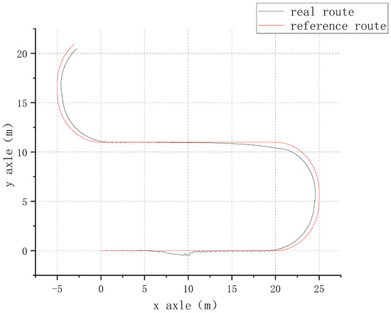
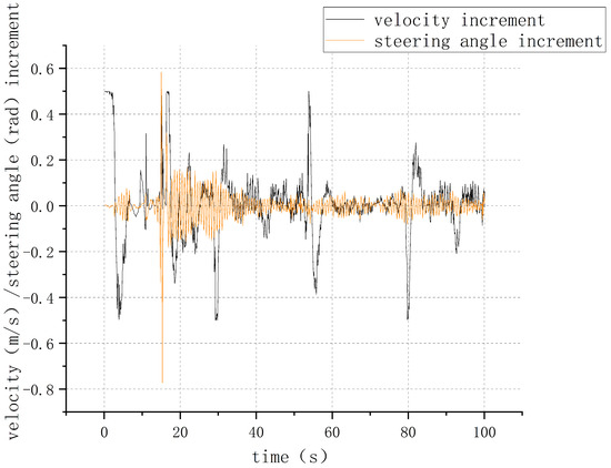
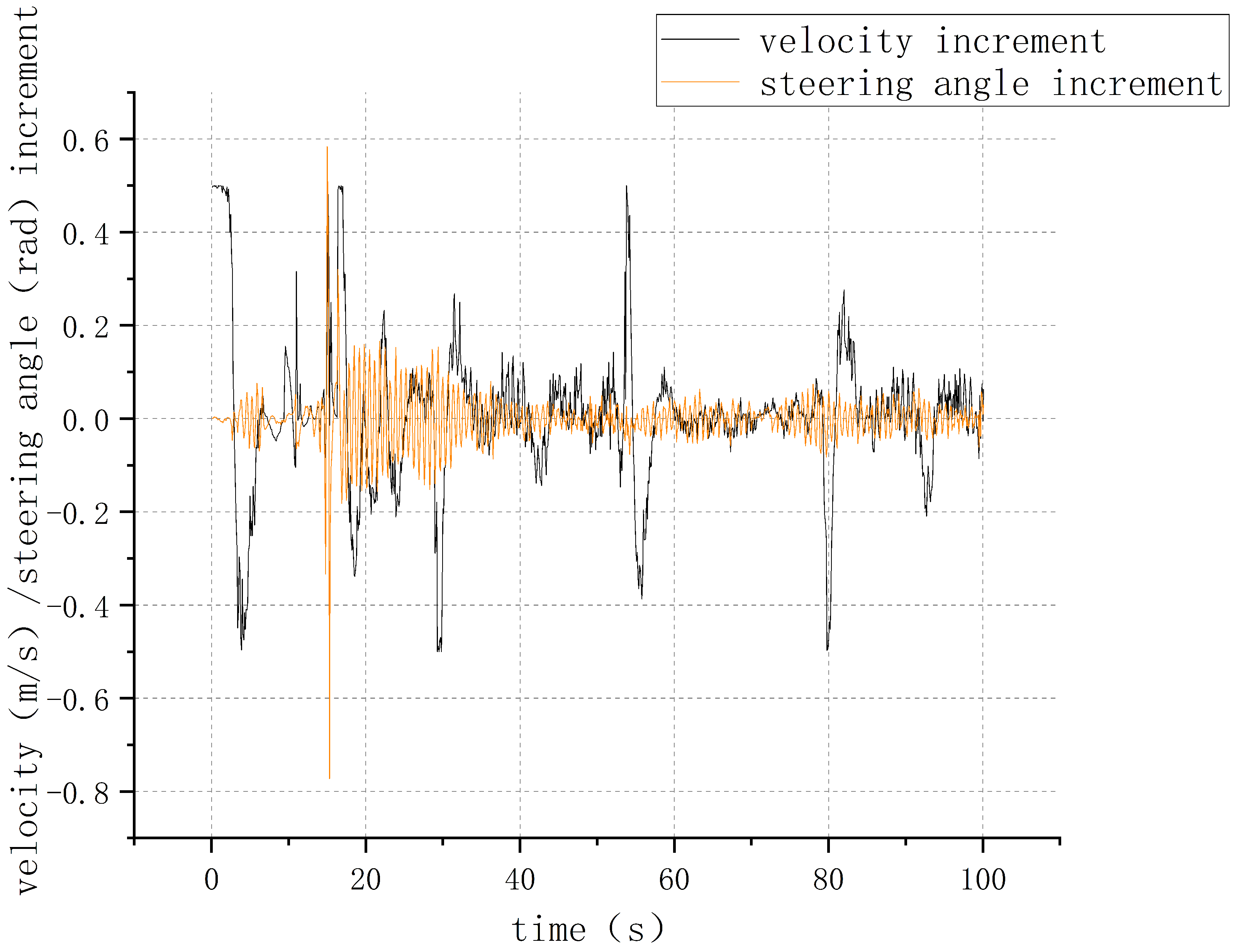
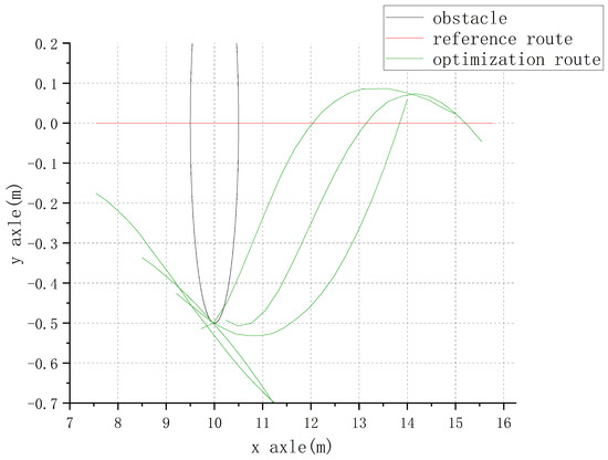
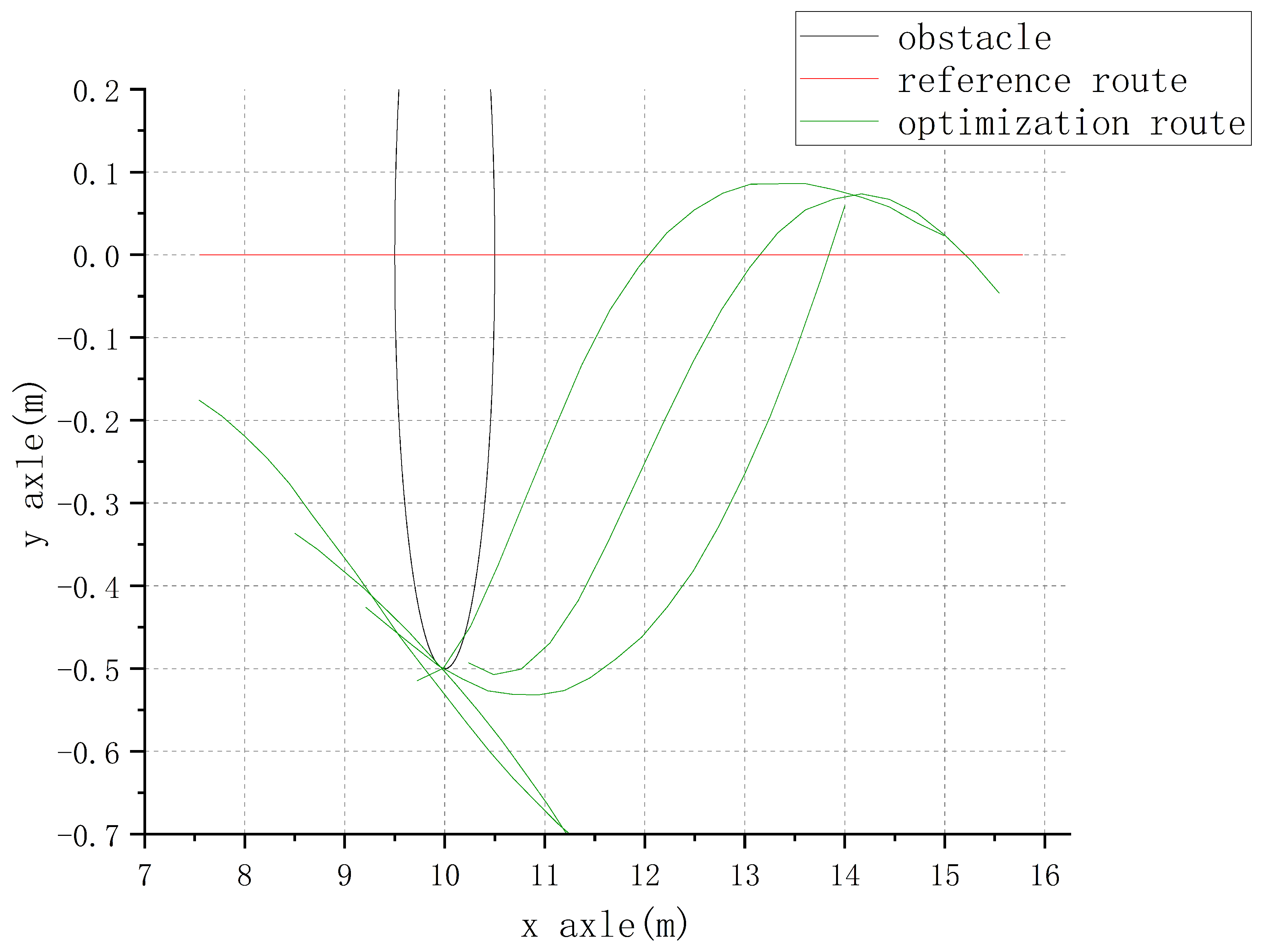
The controller’s path-tracking and obstacle-avoidance capabilities are evaluated using the parameters in Table 2. The results are shown in Figure 12, Figure 13, Figure 14, Figure 15 and Figure 16.

Figure 12. Actual vs. reference path of the tractor.

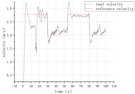
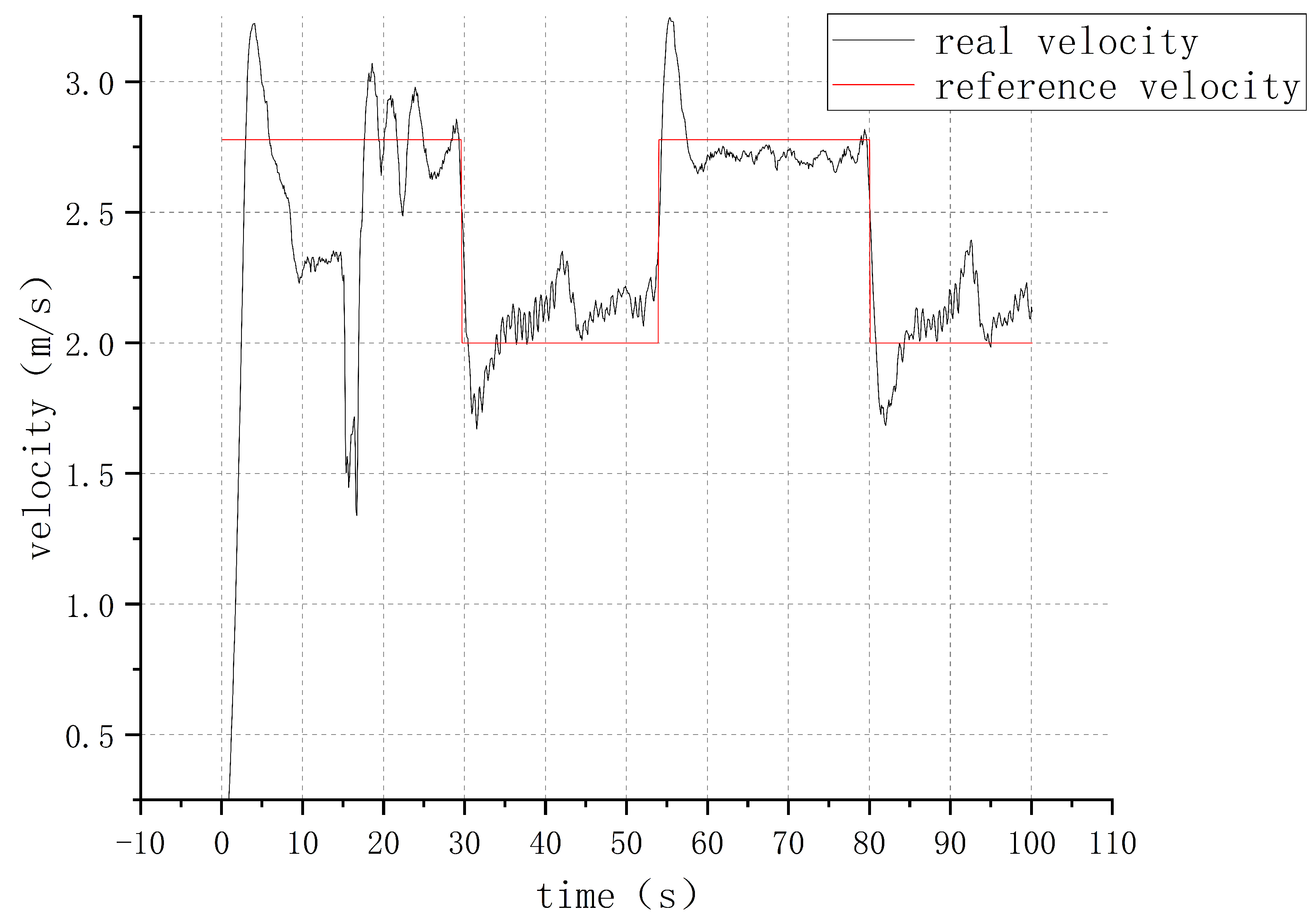
Figure 13. Actual vs. reference velocity of the tractor.

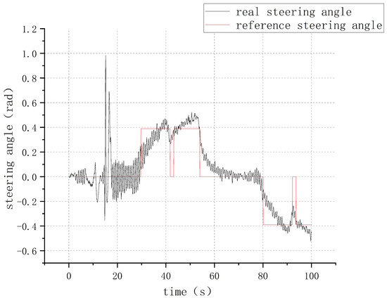
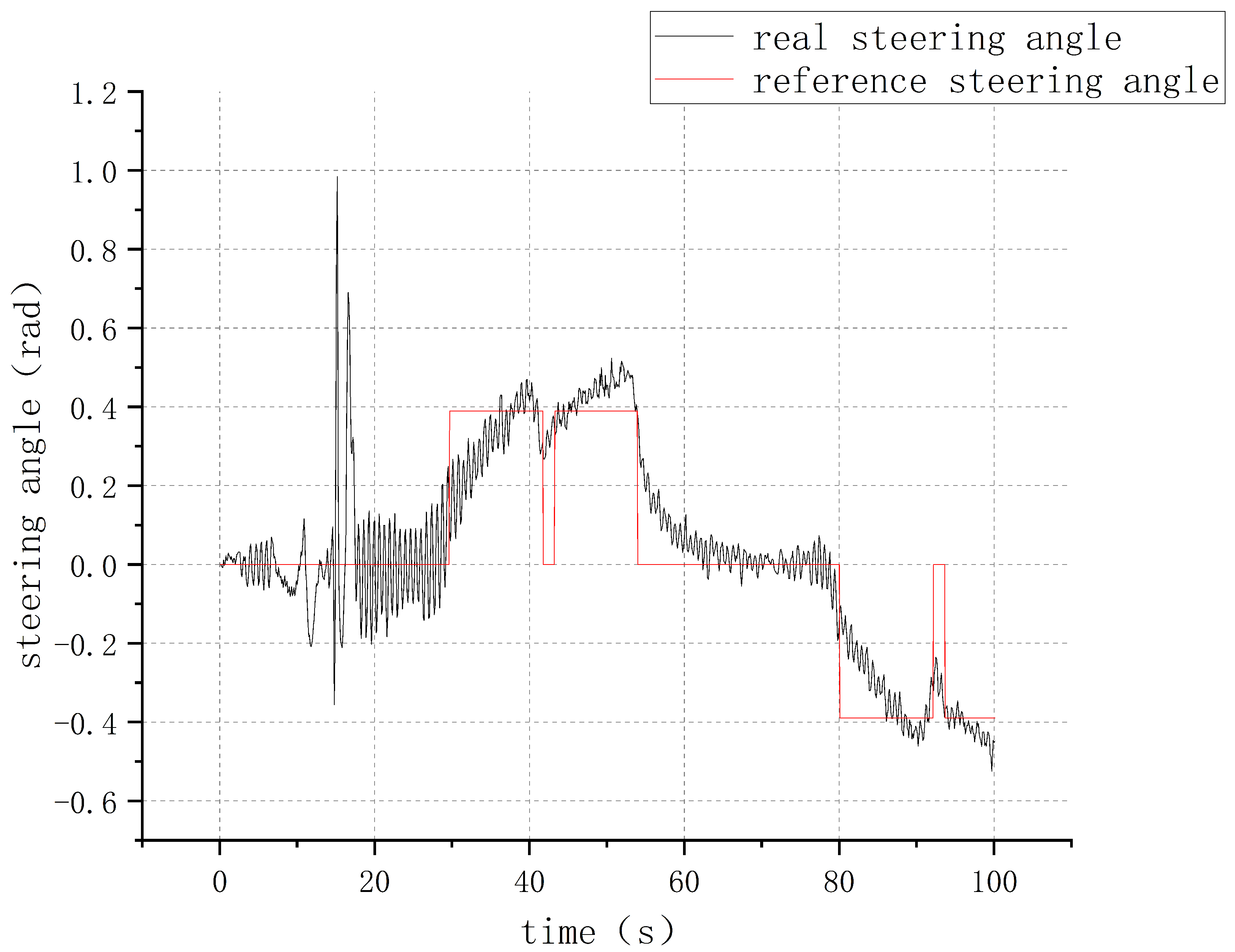
Figure 14. Actual vs. reference steering angle of the tractor.

Figure 15. Control increments: velocity ($▵v$) and steering angle ($▵\delta$).

Figure 16. Obstacle avoidance: optimized predicted trajectories (green), reference path (red), and obstacle (black circle). The actual path is in black.

4.3.1. Path Tracking Accuracy

Figure 12 shows that the tractor accurately follows the reference path comprising straight lines and arcs. The maximum tracking error is approximately 0.2 m during turns, which is primarily attributed to the mismatch between the simplified kinematic model (5) used in the controller and the high-fidelity dynamic model in CarSim. Despite this, the controller demonstrates good robustness and quickly corrects deviations.

4.3.2. Input Tracking and Smoothness

Figure 13 and Figure 14 show that the actual velocity and steering angle closely track their references during unconstrained segments. The transient deviations near the obstacle (at $x\approx 10$ m) are the controller’s active responses for collision avoidance. Figure 15 confirms that the control increments $▵v$ and $▵\delta$ are strictly bounded within the prescribed limits ($\pm 0.5$ m/s and $\pm 1$ rad), ensuring smooth actuator commands, which is crucial for passenger comfort and hardware durability in agricultural vehicles.

4.3.3. Obstacle Avoidance Capability

The obstacle avoidance performance is a key test of the proposed method’s ability to handle non-convex, nonlinear constraints. Figure 16 visualizes the optimized predicted trajectories (green clusters) at several time instants near the obstacle. These trajectories smoothly deviate from the reference path (red) to maintain a safe distance from the obstacle (black circle), demonstrating the effectiveness of the nonlinear penalty function network constructed in Section 3.2 (Figure 11). The resulting actual path (black) successfully circumvents the obstacle, proving the practical viability of solving such complex constrained problems with our NN-based optimization strategy.

4.4. Comparative Analysis

4.4.1. Comparison with Conventional Nonlinear Solvers

To highlight the efficiency of our approach, we attempted to solve the equivalent L2-norm version of problem (9) using conventional optimization algorithms, including local methods (steepest descent, Newton, Quasi-Newton) and global methods (genetic algorithm, particle swarm optimization). For problems with $N_p>5$ or $N_c>5$, none of these solvers could produce a reasonable solution within a practical time frame (e.g., 10 min). This failure underscores the challenge of solving high-dimensional, non-convex NMPC problems with traditional methods. In contrast, our strategy reformulates the optimization as a structured neural network training task, leveraging highly parallelizable and robust gradient-based algorithms. While the solution may be a local optimum, it is computationally tractable and yields satisfactory control performance, making it suitable for practical applications.

4.4.2. Comparison with Linearized MPC (LMPC)

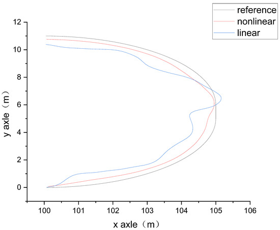
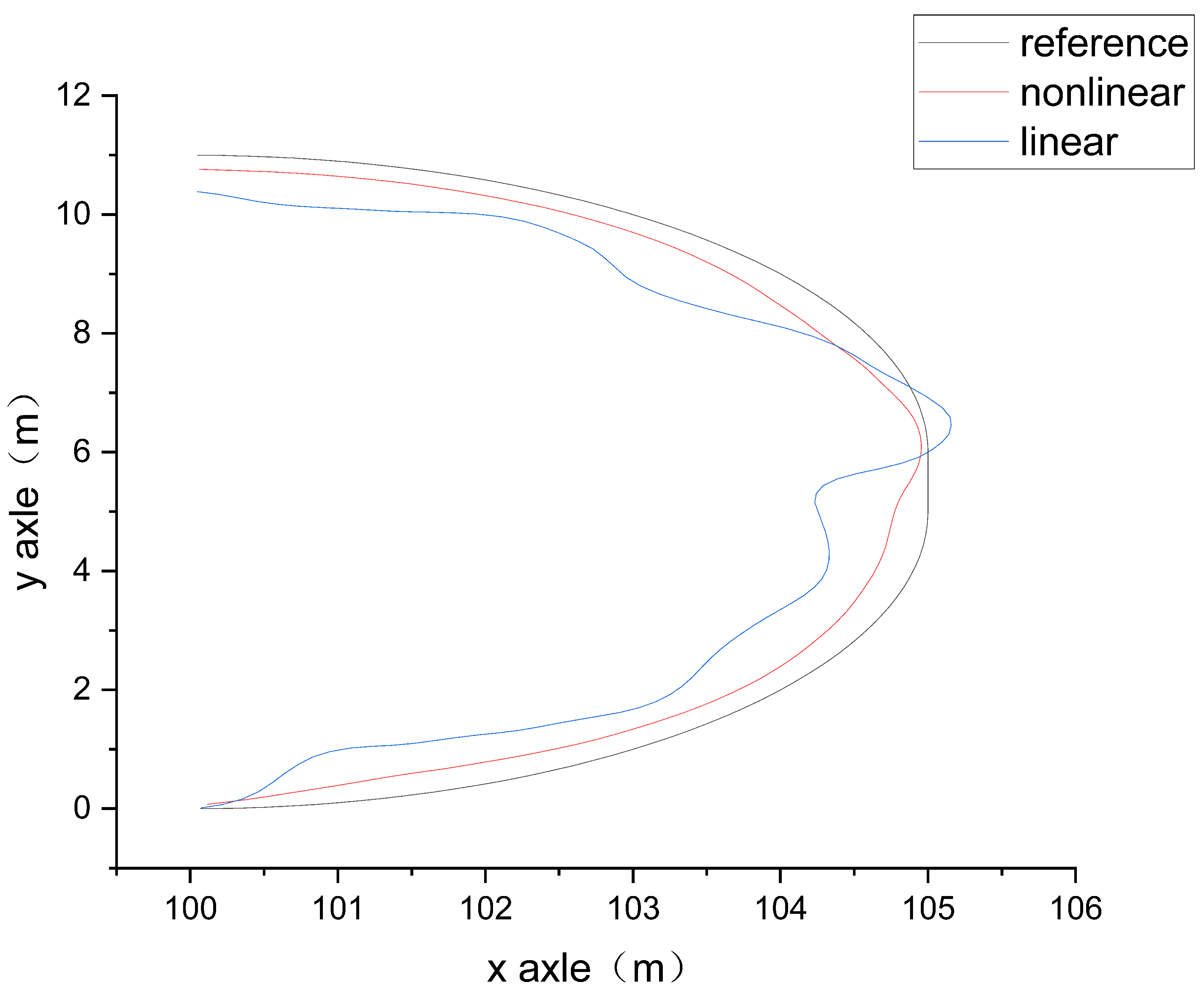
To validate the necessity of the nonlinear model, we compared our NMPC with an LMPC that uses a linearized version of the kinematic model (5) around the reference trajectory. A pure path-tracking scenario (no obstacle) with varying turning radii was tested. Figure 17 and Table 4 present the results.

Figure 17. Path tracking comparison: Nonlinear MPC vs. linearized MPC (Turning radius = 5 m).

Table 4. Average path tracking error: NMPC vs. LMPC.

No.	Turning Radius	Controller Type	Average Tracking Error
1	10 m	Linear	0.354384 m
2	10 m	Nonlinear	0.121985 m
3	7 m	Linear	0.464007 m
4	7 m	Nonlinear	0.166604 m
5	5 m	Linear	0.566659 m
6	5 m	Nonlinear	0.233134 m

Figure 17 clearly shows the superior tracking accuracy of the nonlinear controller (red) over the linearized one (blue), especially during the turn. The linearization error degrades the LMPC’s performance, causing a steady-state offset. Table 4 quantifies this: across all tested turning radii, NMPC reduces the average tracking error by 58.9% to 65.5% compared to LMPC. The advantage becomes more pronounced as the turning radius decreases, highlighting the critical importance of an accurate nonlinear model for high-precision maneuvers like tight headland turns in agricultural operations.

5. Conclusions

This paper has presented a novel and efficient strategy for solving the Nonlinear Model Predictive Control (NMPC) problem by encoding it as a trainable neural network. Unlike prevalent approaches that use neural networks as black-box approximators for the policy or system model, our method constructs an interpretable, white-box computational graph that is mathematically equivalent to the original constrained L1-norm optimization problem. The optimal control sequence is then obtained by performing fast gradient-based training (e.g., backpropagation) on this specifically constructed network, leveraging the parallel computation infrastructure of modern deep learning.

The proposed strategy was successfully applied to the real-time path-tracking control of an autonomous tractor, demonstrating significant advantages in both computational efficiency and control performance. The main contributions of this work are threefold:

• A Paradigm Shift in NMPC Solving: We introduce a new paradigm that transforms the traditional nonlinear programming problem in NMPC into a neural network training task. This allows the challenging, constrained nonlinear optimization to be tackled by highly efficient, parallelizable, and robust off-the-shelf gradient-based optimizers (e.g., Levenberg–Marquardt, Adam), bypassing the need for complex derivative calculations or approximations inherent in conventional solvers.
• A Framework for Interpretable, Exact Problem Encoding: We provide a systematic framework for constructing exact, component-wise neural network equivalents of the NMPC problem, including the nonlinear system dynamics, the L1-norm cost function, and the hard/soft constraints. This results in a transparent and interpretable “optimizer network” rather than a data-driven black box, ensuring the solved control sequence corresponds to the original problem specification without approximation error from pre-training.
• Validation of Real-Time Feasibility and Superiority: Through comprehensive co-simulation tests on a high-fidelity tractor model, we empirically validate that the proposed method:
  • Achieves excellent real-time performance, with solution times on the order of hundreds of milliseconds for horizons up to 20 steps, making direct NMPC applicable to fast motion control.
  • Exhibits a unique scaling property where computation time remains largely insensitive to increases in the control horizon ($N_c$), which is a major advantage over traditional solvers.
  • Significantly outperforms linearized MPC in tracking accuracy, especially during tight maneuvers, by fully utilizing the nonlinear vehicle model.
  • Effectively handles non-convex constraints (e.g., obstacle avoidance) that are notoriously difficult for many nonlinear programming solvers.

Broader Impact and Applications: While demonstrated in the context of agricultural vehicle control, the proposed strategy is general and can be readily extended to other domains where efficient solution of constrained nonlinear optimization is crucial, such as robotics, process control, and energy systems. It also opens a promising avenue for seamlessly integrating analytical (white-box) models with data-driven (black-box) sub-models within a unified, optimizable neural network framework, facilitating the development of advanced compound or robust predictive controllers.

Limitations and Future Work: The current approach’s computational cost scales approximately linearly with the prediction horizon ($N_p$) due to the recursive network structure. A promising direction is to explore weight-sharing architectures, such as Recurrent Neural Networks (RNNs) or Neural Ordinary Differential Equations (Neural ODEs), to represent the system dynamics more compactly across the prediction horizon, potentially decoupling the computational cost from $N_p$. Furthermore, investigating the application of this strategy to Stochastic or Robust MPC by encoding uncertainty sets into the network architecture presents a compelling avenue for future research. Finally, implementation on embedded hardware and experimental validation with a physical tractor are essential next steps toward practical deployment.

In summary, this work bridges the gap between the powerful optimization engines of deep learning and the demanding requirements of real-time NMPC, offering a fresh, efficient, and practical solution for advanced control of complex nonlinear systems.

References

- Zhao, Z.G.; Zhou, L.J.; Zhu, Q. Preview Distance Adaptive Optimization for the Path TrackingControl of Unmanned Vehicle. J. Mech. Eng. 2018, 24, 166–173. [Google Scholar] [CrossRef] [Scilit]
- Lu, Z.X.; Gong, J.H.; Lu, Y. Simulation and Experiment of Dual-Channel PID Control for Tractor Hydraulic Steering System with Drive-by-Wire Technology. Trans. Chin. Soc. Agric. Eng. 2016, 32, 101–106. [Google Scholar]
- Zhang, S.; Liu, J.Y.; Du, Y.F. Automatic Navigation Control Method for Tractors Based on Speed Adaptation. Trans. Chin. Soc. Agric. Eng. 2017, 33, 48–55. [Google Scholar]
- Latif, A.R.; Chalhoub, B.; Pilipchuk, V. Control of the nonlinear dynamics of a truck and trailer combination. Nonlinear Dyn. 2020, 99, 2505–2526. [Google Scholar] [CrossRef] [Scilit]
- Wang, S.D. Research on Tractor Assisted Driving System Based on BeiDou Satellite Navigation; Jiangsu University: Zhenjiang, China, 2017. [Google Scholar]
- Shi, X.; Ma, R.; Zhang, V.L. Simulation Study on Tractor Path Tracking Based on Fuzzy Control. Agric. Mech. Res. 2016, 38, 237–241. [Google Scholar]
- Zhao, X.J.; Zhang, P.P. Real-Time Path Tracking for Intelligent Tractors Based on MPC. Anhui Agric. Sci. 2021, 49, 191–194. [Google Scholar]
- Yue, M.; Hou, X.; Gao, R. Trajectory tracking control for tractor-trailer vehicles: A coordinated control approach. Nonlinear Dyn. 2018, 91, 1061–1074. [Google Scholar] [CrossRef] [Scilit]
- Gao, H.B.; Kan, Z.; Li, K.Q. Robust Lateral Trajectory Following Control of Unmanned Vehicle Based on Model Predictive Control. IEEE-ASME Trans. Mechatron. 2022, 27, 1278–1287. [Google Scholar] [CrossRef] [Scilit]
- Kayacan, E.; Saeys, W.; Ramon, H.; Belta, C.; Peschel, J.M. Experimental Validation of Linear and Nonlinear MPC on an Articulated Unmanned Ground Vehicle. IEEE-ASME Trans. Mechatron. 2013, 23, 2023–2030. [Google Scholar] [CrossRef] [Scilit]
- Wang, L.; Cai, Y.L.; Ding, B.C. Robust Model Predictive Control with Bi-Level Optimization for Boiler-Turbine System. IEEE Access 2021, 9, 48244–48253. [Google Scholar] [CrossRef] [Scilit]
- Xiao, W.; Cassandras, C.G.; Belta, C.A. Bridging the gap between optimal trajectory planning and safety-critical control with applications to autonomous vehicles. Automatica 2021, 129, 109592. [Google Scholar] [CrossRef] [Scilit]
- Zhang, X.J.; Bujarbaruah, M.; Borrelli, F. Near-Optimal Rapid MPC Using Neural Networks: A Primal-Dual Policy Learning Framework. IEEE Trans. Control Syst. Technol. 2021, 29, 2102–2114. [Google Scholar] [CrossRef] [Scilit]
- He, N.; Qi, L.P.; Xu, Z.X.; Du, J.W. Event-Driven Model Predictive Controller for State Constrained Systems: An Input Signal Reconstruction Method. IEEE Access 2021, 9, 74209–74217. [Google Scholar] [CrossRef] [Scilit]
- Hu, Z.R.; Shi, P.; Wu, L.G. Polytopic Event-Triggered Robust Model Predictive Control for Constrained Linear Systems. IEEE Trans. Circuits Syst. I-Regul. Pap. 2021, 68, 2594–2603. [Google Scholar] [CrossRef] [Scilit]
- Li, P.F.; Kang, Y.; Zhao, Y.B.; Wang, T. A Novel Self-Triggered MPC Scheme for Constrained Input-Affine Nonlinear Systems. IEEE Trans. Circuits Syst. II-Express Briefs 2021, 68, 306–310. [Google Scholar] [CrossRef] [Scilit]
- Sun, Z.Q.; Dai, L.; Xia, Y.Q.; Liu, K. Event-Based Model Predictive Tracking Control of Nonholonomic Systems with Coupled Input Constraint and Bounded Disturbances. IEEE Trans. Autom. Control 2018, 63, 608–615. [Google Scholar] [CrossRef] [Scilit]
- Zhang, H.; Zhang, H.M.; Wang, Z.P.; Huang, C.; Li, Y. Adaptive event based predictive lateral following control for unmanned ground vehicle system. Int. J. Robust Nonlinear Control. 2021, 31, 4744–4763. [Google Scholar] [CrossRef] [Scilit]
- Ji, J.H.; Jin, S.B.; Zhao, W.X.; Xu, D.Z.; Huang, L.S.; Qiu, X.Q. Simplified Three-Vector-Based Model Predictive Direct Power Control for Dual Three-Phase PMSG. IEEE Trans. Energy Convers. 2022, 37, 1145–1155. [Google Scholar] [CrossRef] [Scilit]
- Pang, S.W.; Li, Q.H.; Ni, B. Improved nonlinear MPC for aircraft gas turbine engine based on semi-alternative optimization strategy. Aerosp. Sci. Technol. 2021, 118, 106983. [Google Scholar] [CrossRef] [Scilit]
- Wang, H.R.; Wang, Q.D.; Chen, W.W.; Zhao, L.F.; Tan, D.K. Path tracking based on model predictive control with variable predictive horizon. Trans. Inst. Meas. Control 2021, 43, 2676–2688. [Google Scholar] [CrossRef] [Scilit]
- Moriyasu, R.; Ikeda, T.; Kawaguchi, S.; Kashima, K. Structured Hammerstein-Wiener Model Learning for Model Predictive Control. IEEE Control Syst. Lett. 2022, 6, 397–402. [Google Scholar] [CrossRef] [Scilit]
- Wang, Z.P.; Li, G.B.; Jiang, H.J.; Chen, Q.J.; Zhang, H. Collision-Free Navigation of Autonomous Vehicles Using Convex Quadratic Programming-Based Model Predictive Control. IEEE-ASME Trans. Mechatron. 2018, 23, 1103–1113. [Google Scholar] [CrossRef] [Scilit]
- Abu-Ali, M.; Berkel, F.; Manderla, M.; Reimann, S.; Kennel, R.; Abdelrahem, M. Deep Learning-Based Long-Horizon MPC: Robust, High Performing, and Computationally Efficient Control for PMSM Drives. IEEE Trans. Power Electron. 2022, 37, 12486–12501. [Google Scholar] [CrossRef] [Scilit]
- Krishnamoorthy, D.; Mesbah, A.; Paulson, J.A. An adaptive correction scheme for offset-free asymptotic performance in deep learning-based economic mpc. IFAC PapersOnLine 2021, 54, 584–589. [Google Scholar] [CrossRef] [Scilit]
- Lovelett, R.J.; Dietrich, F.; Lee, S.; Kevrekidis, I.G. Some manifold learning considerations toward explicit model predictive control. Aiche J. 2020, 66, e16881. [Google Scholar] [CrossRef] [Scilit]
- Reda, A.; Bouzid, A.; Vasarhelyi, J. Deep Learning-Based Automated Vehicle Steering. In Proceedings of the 2021 22nd International Carpathian Control Conference (ICCC), Ostrava, Czech Republic, 31 May–1 June 2021. [Google Scholar] [CrossRef] [Scilit]
- Vaupel, Y.; Hamacher, N.C.; Caspari, A.; Mhamdi, A.; Kevrekidis, I.G.; Mitsos, A. Accelerating nonlinear model predictive control through machine learning. J. Process Control 2020, 92, 261–270. [Google Scholar] [CrossRef] [Scilit]
- Wang, G.M.; Qiao, J.F.; Liu, C.X.; Shen, Z.X. How Deep Is Deep Enough for Deep Belief Network for Approximating Model Predictive Control Law. IEEE Trans. Autom. Sci. Eng. 2022, 19, 2067–2078. [Google Scholar] [CrossRef] [Scilit]
- Wang, S.D.; Dragicevic, T.; Gontijo, G.F.; Chaudhary, S.K.; Teodorescu, R. Machine Learning Emulation of Model Predictive Control for Modular Multilevel Converters. IEEE Trans. Ind. Electron. 2021, 68, 11628–11634. [Google Scholar] [CrossRef] [Scilit]
- Hewing, L.; Wabersich, K.P.; Menner, M.; Zeilinger, M.N. Learning-Based Model Predictive Control: Toward Safe Learning in Control. Annu. Rev. Control Robot. Auton. Syst. 2020, 3, 269–296. [Google Scholar] [CrossRef] [Scilit]
- Dong, L.; Yan, J.; Yuan, X.; He, H.B.; Sun, C.Y. Functional Nonlinear Model Predictive Control Based on Adaptive Dynamic Programming. IEEE Trans. Cybern. 2019, 49, 4206–4218. [Google Scholar] [CrossRef] [Scilit] [PubMed]
- Kang, T.; Peng, H.; Xu, W.Q.; Sun, Y.P.; Peng, X.Y. Deep Learning-Based State-Dependent ARX Modeling and Predictive Control of Nonlinear Systems. IEEE Access 2023, 11, 32579–32594. [Google Scholar] [CrossRef] [Scilit]
- Manzoor, T.; Pei, H.L.; Sun, Z.Q.; Cheng, Z.H. Model Predictive Control Technique for Ducted Fan Aerial Vehicles Using Physics-Informed Machine Learning. Drones 2023, 7, 4. [Google Scholar] [CrossRef] [Scilit]
- Wang, G.M.; Jia, Q.S.; Qiao, J.F.; Bi, J.; Zhou, M.C. Deep Learning-Based Model Predictive Control for Continuous Stirred-Tank Reactor System. IEEE Trans. Neural Netw. Learn. Syst. 2021, 32, 3643–3652. [Google Scholar] [CrossRef] [Scilit] [PubMed]
- Wu, Z.; Rincon, D.; Gu, Q.Q.; Christofides, P.D. Statistical Machine Learning in Model Predictive Control of Nonlinear Processes. Mathematics 2021, 9, 1912. [Google Scholar] [CrossRef] [Scilit]
- Bistarelli, S.; Faltings, B.; Neagu, N. Interchangeability with thresholds and degradation factors for Soft CSPs. Ann. Math. Artif. Intell. 2013, 67, 123–163. [Google Scholar] [CrossRef] [Scilit]
- Febbo, H.; Liu, J.; Jayakumar, P.; Stein, J.L.; Ersal, T. Moving Obstacle Avoidance for Large, High-Speed Autonomous Ground Vehicles. In Proceedings of the American Control Conference, Seattle, WA, USA, 24–26 May 2017. [Google Scholar] [CrossRef] [Scilit]
- Kerrigan, E.C.; Maciejowski, J.M. Soft constraints and exact penalty functions in model predictive control. In Proceedings of the UKACC International Conference on CONTROL 2000 Proceedings of International Conference on Control 2000, London, UK, 4–7 September 2000. [Google Scholar]
- Mayne, D.Q.; Rawlings, J.B.; Rao, C.V.; Scokaert, P.O.M. Constrained model predictive control: Stability and optimality. Automatica 2000, 36, 789–814. [Google Scholar] [CrossRef] [Scilit]
- Oravec, J.; Bakosova, M. Soft constraints in the robust MPC design via LMIs. In Advances in Computing and Communications; IEEE: New York, NY, USA, 2016. [Google Scholar]
- Introduction to CarSim. 2021. Available online: https://www.carsim.com/downloads/pdf/CarSim_Introduction.pdf (accessed on 1 July 2025).
Disclaimer/Publisher’s Note: The statements, opinions and data contained in all publications are solely those of the individual author(s) and contributor(s) and not of MDPI and/or the editor(s). MDPI and/or the editor(s) disclaim responsibility for any injury to people or property resulting from any ideas, methods, instructions or products referred to in the content. |
© 2026 by the authors. Licensee MDPI, Basel, Switzerland. This article is an open access article distributed under the terms and conditions of the Creative Commons Attribution (CC BY) license.