Attention-Enhanced YOLOv26 with Tree-Structured Parzen Estimator Optimization for Robust Dental Surgical Tool Detection

Abstract

Object detection remains a fundamental challenge in computer vision and plays a pivotal role in safety-critical medical applications, including surgical instrument recognition and operating-room workflow automation. This study presents a comprehensive comparative evaluation of five attention mechanisms—Squeeze-and-Excitation (SE), Convolutional Block Attention Module (CBAM), Efficient Channel Attention (ECA), Simple Attention Module (SimAM), and an enhanced multi-kernel Spatial Pyramid Pooling Fast module (SPPF+)—integrated into the YOLOv26n backbone, together with two neck-level attention variants (ECA-Neck and CBAM-Neck). A total of 16 model configurations were systematically investigated on a 22-class dental surgical instrument detection dataset under both default training settings and hyperparameter configurations optimized using the Optuna Tree-structured Parzen Estimator (TPE), enabling a rigorous full-factorial ablation study. Experimental results demonstrate that TPE-based hyperparameter optimization consistently enhances detection performance across all architectures. Among the evaluated models, CBAM-Opt achieved the highest detection accuracy, attaining an mAP@50 of 0.959 and an F1-score of 0.913, although the margins among the top optimized configurations fall within run-to-run variability. In contrast, Base-Opt delivered the strongest strict-localization capability with an mAP@50–95 of 0.800, highlighting the competitive performance of the baseline architecture when appropriately optimized. Notably, the parameter-free SimAM module exhibited the largest improvement following optimization ($\Delta$mAP@50 = +0.040), indicating a pronounced sensitivity to training configuration. Furthermore, neck-level attention integration achieved performance comparable to backbone-based attention, with ECA-Neck-Opt reaching an mAP@50 of 0.959, suggesting an effective alternative that preserves pretrained feature representations while maintaining high detection accuracy. Beyond performance evaluation, this work provides a unified benchmarking framework for attention mechanisms in medical object detection, accompanied by computational complexity analysis and practical architectural insights. The findings establish evidence-based guidelines for selecting attention modules in resource-aware surgical vision systems and contribute toward the development of more accurate and reliable computer-assisted clinical workflows.

1. Introduction

Object detection is a fundamental computer-vision problem that simultaneously estimates the location and class of every object in an image [1]. With the maturation of deep-learning-based detectors, real-world deployments now span a broad spectrum, ranging from autonomous-driving perception to medical diagnostics. Within this landscape, the You Only Look Once (YOLO) family [1]—introduced as a single-stage alternative to costly region-proposal pipelines—has become the de facto real-time object-detection standard. Successive generations from YOLOv5 [2] through YOLOv26 [3] have progressively refined the balance between accuracy and computational efficiency.

In the medical imaging context, automatic surgical tool detection is critical both for the safety of robotic surgical systems and for operating-room workflow automation [4]. A misidentified or missed instrument can lead to life-threatening complications [5]. The dental surgical setting is particularly demanding: more than 20 visually similar metallic instrument classes, partial occlusion, specular highlights and variable illumination make reliable detection difficult [6,7]. This background creates a clear demand for lightweight detection models that combine high accuracy with real-time inference.

Attention mechanisms have been widely adopted to increase the capacity of deep networks to selectively focus on the most informative spatial and channel features [8]. The Squeeze-and-Excitation (SE) block [9] was the first widely adopted architecture for explicit channel attention; it was subsequently extended with spatial attention by CBAM [10]; ECA [11] reduced the parameter cost of SE to $O(logC)$; and SimAM [12] introduced fully parameter-free analytical 3D attention. For readers less familiar with computer-vision terminology, these four modules (SE, CBAM, ECA and SimAM) represent the canonical families of channel- and spatial-attention designs, and a consolidated list of all abbreviations used in this manuscript is provided in the Abbreviations section for ease of reference. Although such modules have produced strong results when transplanted into medical object detectors [13,14,15], a comprehensive head-to-head comparison tailored to dental surgical tool detection has not yet appeared in the literature.

Hyperparameter optimization is a second critical factor that directly influences model performance. Bayesian optimization [16] and especially Tree-structured Parzen Estimator (TPE) [17] enable efficient discovery of hyperparameter configurations in high-dimensional search spaces. Optuna [18] provides a modern, define-by-run interface that integrates with deep-learning training pipelines. Nevertheless, systematic studies that jointly evaluate attention mechanisms and hyperparameter optimization remain rare.

Motivated by these gaps, this study seeks to answer the following research questions: (i) Can different attention mechanisms produce measurable performance gains on YOLOv26n? (ii) How do backbone-level versus neck-level attention integration strategies differ in their outcomes? (iii) To what extent does hyperparameter optimization modulate the effectiveness of an attention mechanism? (iv) Which architecture is best suited for dental surgical tool detection?

The original contributions of this work are summarized as follows:

• A systematic ablation of five attention mechanisms and two neck-level variants on the YOLOv26n backbone.
• The first large-scale comparative study of backbone-level versus neck-level attention integration in this setting.
• Quantitative evidence of the differential effect of Optuna TPE optimization on each architecture.
• Documentation of the near-identity initialization strategy as a weight-preservation mechanism in transfer learning.
• An evidence-based architectural-selection guideline for clinical deployment.

The remainder of this paper is organized as follows. Section 2 reviews related work. Section 3 presents the dataset, the YOLOv26n baseline architecture, and the attention modules. Section 4 reports the experimental results. Section 5 discusses the findings. Section 6 outlines the study limitations. Section 7 concludes the paper and suggests future research directions.

2. Related Work

Since the original YOLO architecture proposed by Redmon et al. [1] in 2016, the family has evolved into a single-stage, end-to-end alternative to costly region-proposal detectors. Subsequent generations progressively advanced this paradigm: YOLOv7 [19] adopted a trainable bag-of-freebies, YOLOv9 [20] introduced Programmable Gradient Information (PGI) to mitigate information loss, and YOLOv10 [21] removed the non-maximum-suppression (NMS) post-processing step to enable fully end-to-end detection. Sapkota and Karkee [3] provide a comprehensive review of the architectural evolution from YOLOv5 to YOLOv26.

The comprehensive systematic review by Ragab et al. [14], covering 2018–2023, documents the rapid adoption of YOLO-based methods in radiology, pathology and surgery. For surgical tool detection, Wang et al. [22] applied YOLOv4, Jiang et al. [23] used a customized YOLOv5, Ran et al. [24] employed YOLOv7x, and Liu et al. [25] proposed YOLOv7-RepFPN for embedded deployment. A broader systematic review by Ahmed et al. [4] addresses the current state of deep-learning-based surgical instrument recognition and segmentation.

Sivari et al. [7] provided a systematic review of deep-learning methods for dental anomaly diagnosis and highlighted the success of YOLO-based models. Poomrittigul et al. [6] recently introduced a YOLOv8-based dental surgical tool detection model and a pilot benchmark for the field. Beser et al. [26] demonstrated YOLO-based dental detection on panoramic radiographs in mixed dentition, and Lee et al. [27] applied deep learning to early caries detection in bitewing radiographs.

Niu et al. [8] provided a comprehensive review of attention mechanisms. SE [9], CBAM [10], ECA [11] and SimAM [12] represent four canonical channel/spatial-attention designs with distinct compute–cost trade-offs. A medical-imaging-specific evaluation was carried out by Goncalves et al. [15], and Chien et al. [13] combined attention mechanisms with YOLOv8. These studies show that the optimal attention design depends strongly on the task context.

Bayesian optimization [16] and TPE [17] replace manual trial-and-error with a systematic search strategy; Optuna [18] makes this algorithm practical inside modern deep-learning workflows. Compared with random search [28], TPE is especially advantageous in high-dimensional spaces because it exploits the information of previously evaluated trials. The number of studies that combine TPE hyperparameter optimization with attention mechanisms for YOLO-based object detection is still limited, motivating the present work.

Beyond CNN-based single-stage detectors, transformer-based architectures have recently emerged as a competitive detection paradigm. DEtection TRansformer (DETR) [29] reformulated object detection as a direct set-prediction problem and eliminated hand-crafted components such as anchor generation and non-maximum suppression, while real-time variants such as RT-DETR [30] have substantially narrowed the latency gap with YOLO-family detectors. However, transformer-based detectors generally require considerably larger training corpora and higher memory budgets to attain their full accuracy, which is a practical constraint in the data-limited and resource-constrained dental-surgery setting targeted here. For this reason, the present study focuses on a lightweight CNN-based YOLO backbone, and a systematic comparison against transformer-based detectors is identified as a promising direction for future work.

3. Materials and Methods

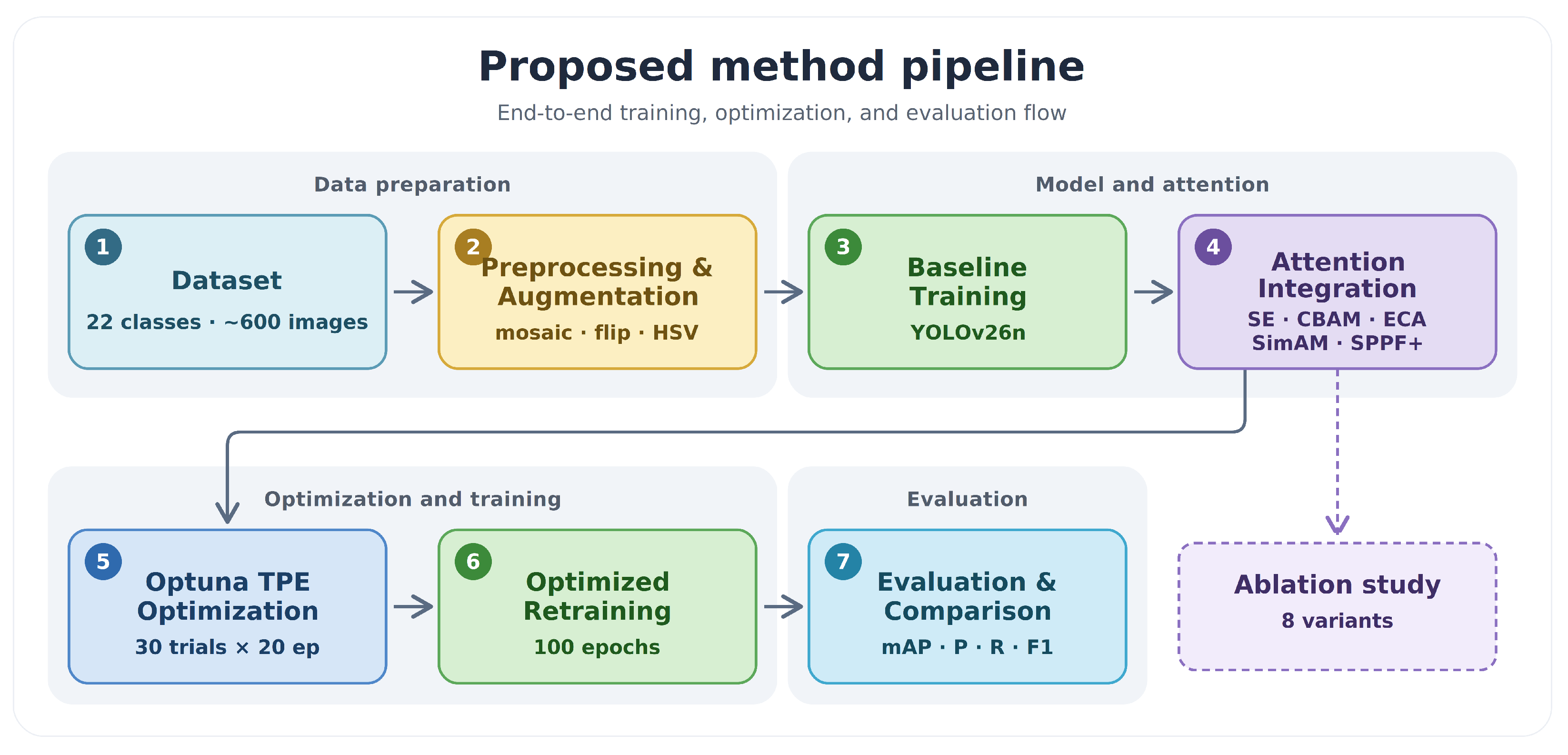
The proposed pipeline, depicted in Figure 1, comprises two principal phases: (i) an attention mechanism ablation study and (ii) Optuna-based hyperparameter optimization. In Phase I, eight architectural variants are trained for 100 epochs under identical default hyperparameters. In Phase II, a single Optuna study of 30 trials is run on the baseline architecture, and the resulting best configuration is applied to every variant and retrained for a full 100 epochs. An overview of the proposed methodology is depicted in Figure 1.

3.1. Dataset

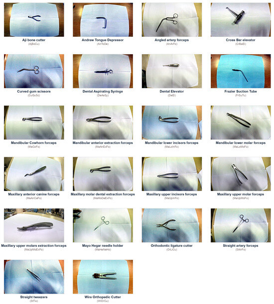
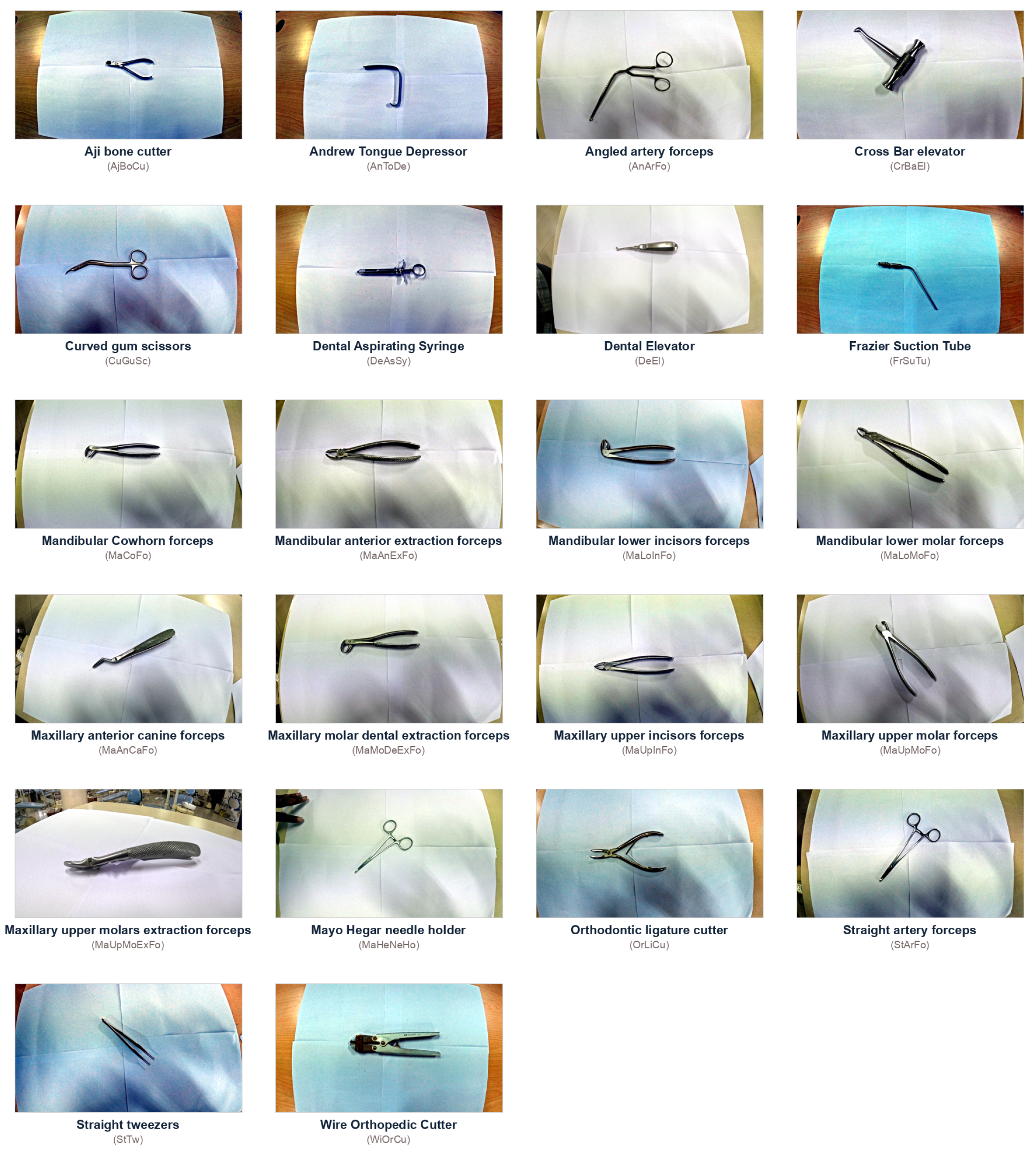
The Annotated Dental Instrument Dataset for YOLO Object Detection [31] was used in this study. It comprises 22 dental surgical instrument classes: Aji bone cutter, Andrew tongue depressor, Angled artery forceps, Cross-bar elevator, Curved gum scissors, Dental aspirating syringe, Dental elevator, Frazier suction tube, Mandibular cowhorn forceps, Mandibular anterior extraction forceps, Mandibular lower incisors forceps, Mandibular lower molar forceps, Maxillary anterior canine forceps, Maxillary molar dental extraction forceps, Maxillary upper incisors forceps, Maxillary upper molar forceps, Maxillary upper molars extraction forceps, Mayo–Hegar needle holder, Orthodontic ligature cutter, Straight artery forceps, Straight tweezers, and Wire orthopaedic cutter. A representative sample image of each class, together with the abbreviation code used for it in the class-level analysis, is shown in Figure 2. Training, validation and test partitions are automatically generated. High visual similarity between classes (in particular among the various extraction-forceps types), partial occlusion and variable illumination make the dataset a realistic and challenging benchmark. All images are annotated in YOLOv26 format and resized to 640 × 640 px.

Figure 3. Normalized confusion matrix of the CBAM-Opt model on the 22-class test split. Values along the diagonal indicate the per-class true-positive rate.

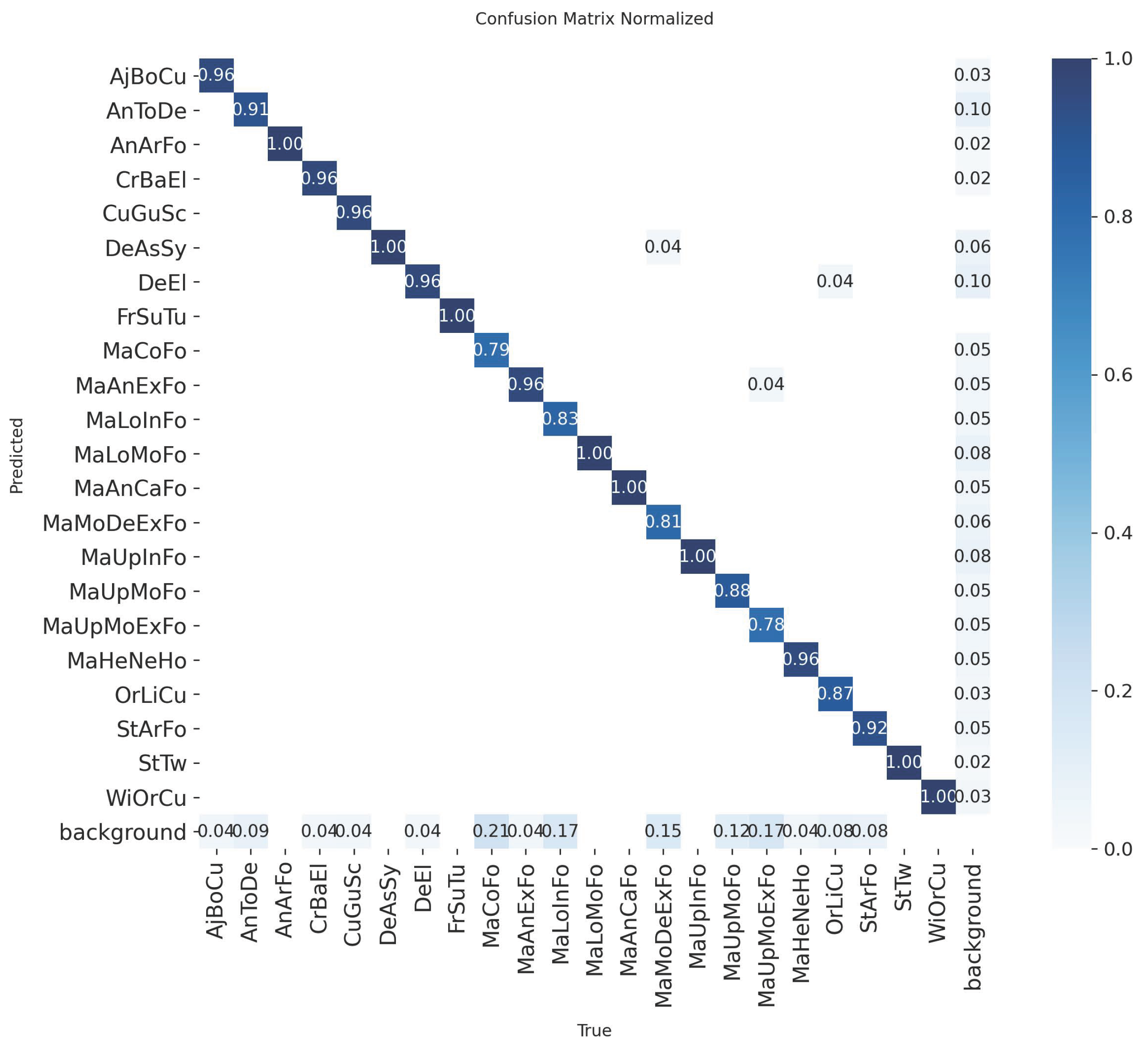
Figure 3. Normalized confusion matrix of the CBAM-Opt model on the 22-class test split. Values along the diagonal indicate the per-class true-positive rate.

3.2. Data-Augmentation Strategy

The augmentation pipeline consists of mosaic (four-image composition), horizontal flip, hue–saturation–value perturbations (HSV-S and HSV-V), translation, scaling, MixUp and Copy-Paste. Mosaic augmentation is especially effective at exposing the network to small and rare instrument classes; Copy-Paste contributes to class-imbalance mitigation. A subset of these parameters is also included in the Optuna search space presented in

Table 1. Optuna TPE hyperparameter search space.

Parameter	Range	Description	Type
lr0	Log-Uniform [1 × ${10}^{-4}$, 1 × ${10}^{-1}$]	Initial learning rate	Continuous
momentum	Uniform [0.70, 0.99]	AdamW ${\beta }_1$	Continuous
weight_decay	Log-Uniform [1 × ${10}^{-5}$, 1 × ${10}^{-2}$]	L2 regularization	Continuous
batch	{16, 32, 48, 64}	Batch size	Discrete
warmup_epochs	Uniform [1.0, 5.0]	Warmup duration	Continuous
hsv_s	Uniform [0.0, 1.0]	Saturation augmentation	Continuous
hsv_v	Uniform [0.0, 1.0]	Value augmentation	Continuous
translate	Uniform [0.0, 0.2]	Translation augmentation	Continuous
scale	Uniform [0.0, 0.9]	Scale augmentation	Continuous
fliplr	Uniform [0.0, 1.0]	Horizontal flip prob.	Continuous
mixup	Uniform [0.0, 0.3]	MixUp probability	Continuous
copy_paste	Uniform [0.0, 0.3]	Copy-Paste probability	Continuous
label_smoothing	Uniform [0.0, 0.1]	Label smoothing eps	Continuous

.

3.3. YOLOv26n Baseline Architecture

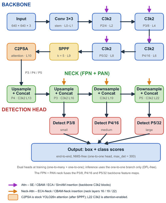
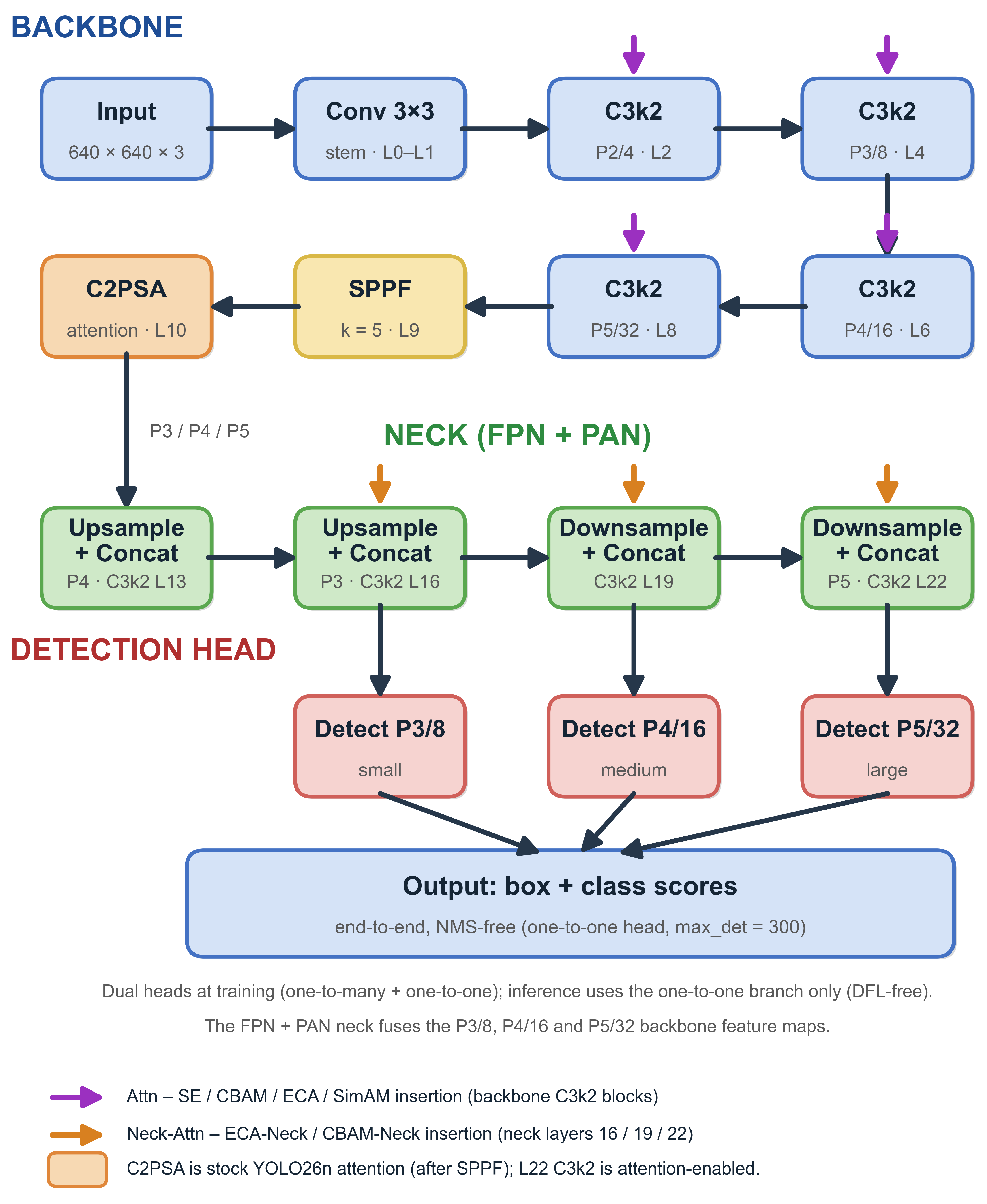
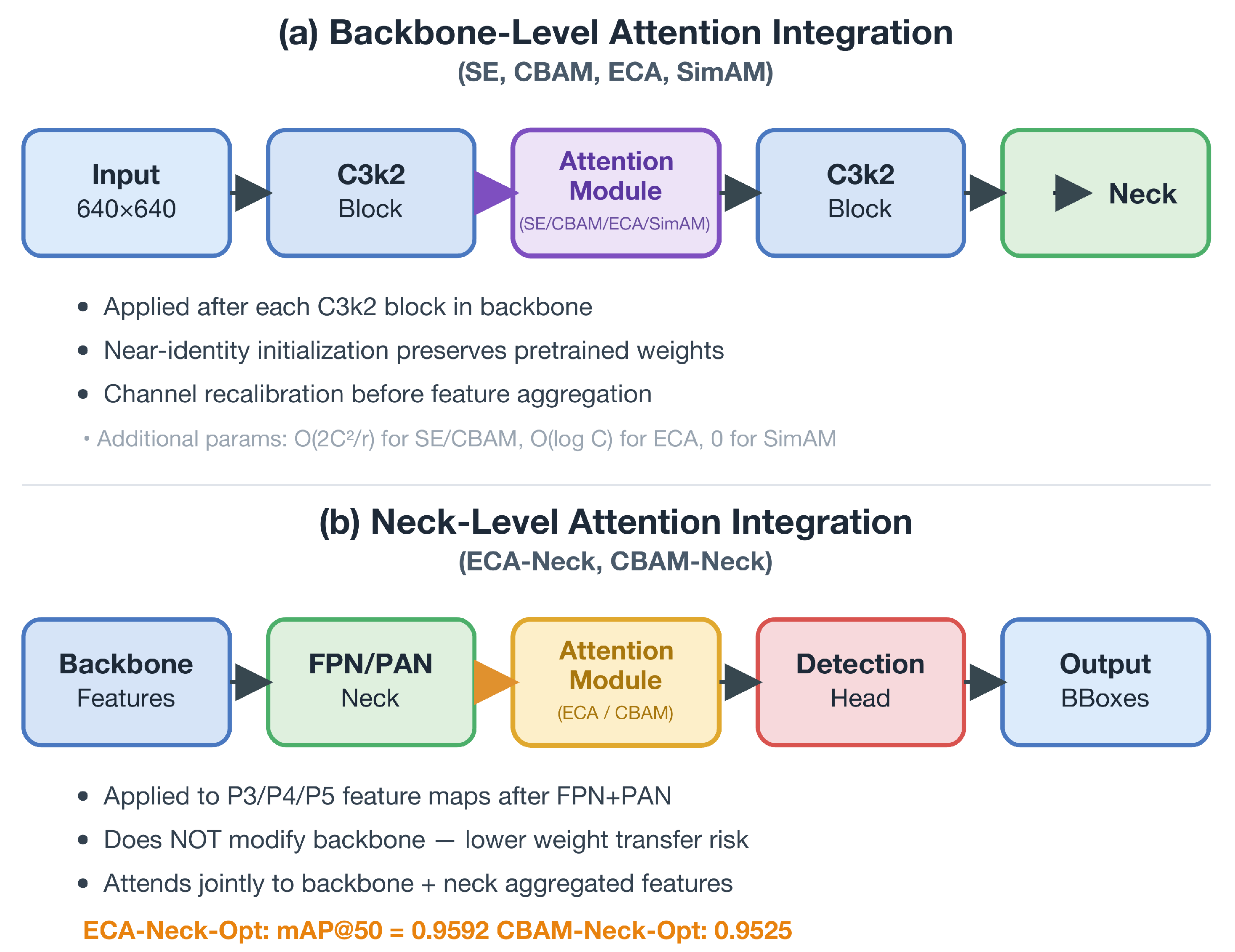
As shown in Figure 4, YOLOv26n [32] is composed of three principal components. The backbone produces multi-scale feature maps through residually connected C3k2 blocks. The neck combines the Feature Pyramid Network (FPN) [33] and the Path Aggregation Network (PANet) [34] to fuse features at the P3/8, P4/16 and P5/32 resolutions. The detection head finally produces class and bounding-box predictions from these maps. The model is trained with GIoU/CIoU regression loss; all attention modules are initialized with a near-identity strategy, preserving the pretrained weights through the early training epochs.

The choice of YOLOv26n as the baseline warrants clarification, as the object-detection community is at present more widely familiar with releases up to YOLO11. YOLOv26 is the most recent generation of the Ultralytics YOLO family [32,35], released as the direct successor to YOLO11 while retaining the same modular backbone–neck–head design philosophy, refined C3k2 feature-extraction blocks, and an updated training pipeline. Architecturally, YOLOv26 differs from earlier generations through a DFL-free, dual-head detection design that enables native non-maximum-suppression (NMS)-free, end-to-end inference: a one-to-many branch provides dense supervision during training, whereas a one-to-one branch, used by default at inference, produces a fixed-size prediction set without NMS, together with a lighter regression head of unconstrained range [35]. Notably, the YOLOv26 backbone already integrates a position-sensitive self-attention block (C2PSA) after the SPPF stage; the present study, therefore, assesses whether adding lightweight channel- and spatial-attention modules (SE, CBAM, ECA and SimAM) on top of this baseline yields further gains. Its training pipeline further couples three complementary components, namely the MuSGD optimizer, Progressive Loss (which gradually shifts supervision from the one-to-many to the one-to-one head), and Small-Target-Aware Label Assignment (STAL, which guarantees positive-sample coverage for tiny objects); the last of these is especially pertinent to the small, slender dental instruments targeted in this study. As documented in the comparative overview of Sapkota and Karkee [3], the YOLO lineage from YOLOv5 through YOLOv26 preserves a high degree of architectural continuity, so that attention-integration findings obtained on YOLOv26n are expected to remain broadly applicable to neighboring generations. We adopt the nano (n) variant specifically because its low parameter budget (2.60 M parameters, 8.2 GFLOPs) matches the resource constraints of clinical edge-deployment scenarios, making it the most relevant baseline for the resource-aware surgical-vision setting considered in this study.

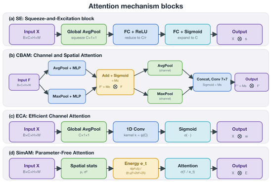
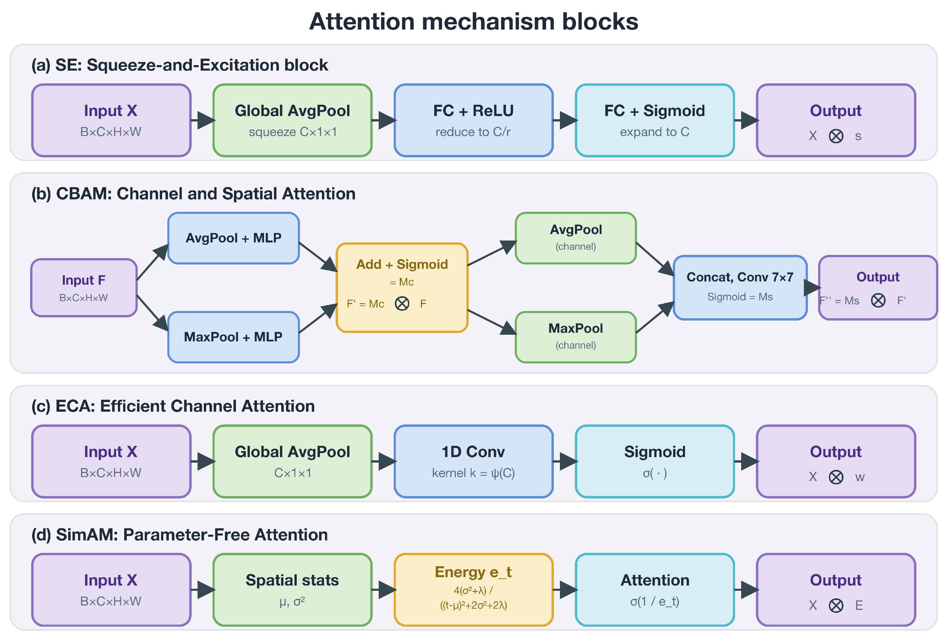
Figure 5 presents the block diagrams of the four attention modules side by side.

3.4. Attention Mechanisms and Mathematical Foundations

The following subsections describe each module’s mathematical foundation, tensor-dimension analysis, computational cost and near-identity initialization scheme.

3.4.1. Squeeze-and-Excitation (SE) Block

For an input feature map $X\in {\mathbb{R}}^{B\times C\times H\times W}$, the SE block [9] first squeezes the spatial dimensions via global average pooling to produce $z\in {\mathbb{R}}^{B\times C}$; two fully connected layers then learn the channel attention weights $s\in {\mathbb{R}}^{B\times C}$

$$z_c={\displaystyle \frac{1}{HW}}{\displaystyle \sum _{i=1}^H}{\displaystyle \sum _{j=1}^W}{u}_c(i,j)$$

(1)

$$s=\sigma \left(W_2\delta \left(W_{1}z\right)\right)$$

(2)

$${\widehat{x}}_c=s_c·u_c$$

(3)

where $\delta$ denotes ReLU and $\sigma$ the sigmoid activation, $W_1\in {\mathbb{R}}^{{\displaystyle \frac{C}{r}}\times C}$ and $W_2\in {\mathbb{R}}^{C\times {\displaystyle \frac{C}{r}}}$ are the fully connected weights, and $r\in \{8,16\}$ is the reduction ratio. Near-identity initialization: $W_1\sim$ Kaiming normal, $W_2.\mathrm{weight}=0$, $W_2.\mathrm{bias}=1\to \mathrm{sigmoid}\left(1\right)\approx 0.73$. Parameter cost: $O(2C^2/r)$. Computational complexity: $O(C^2/r)$.

3.4.2. Convolutional Block Attention Module (CBAM)

CBAM [10] applies channel attention and spatial attention sequentially and, therefore, performs a more comprehensive feature recalibration than SE,

$$M_c\left(F\right)=\sigma \left(\mathrm{MLP}\left(\mathrm{AvgPool}\left(F\right)\right)+\mathrm{MLP}\left(\mathrm{MaxPool}\left(F\right)\right)\right)$$

(4)

$$F^{\prime }=M_c\left(F\right)\otimes F$$

(5)

$$M_s\left(F^{\prime }\right)=\sigma \left(f^{7\times 7}\left(\left[{\mathrm{AvgPool}}_{ch}\left(F^{\prime }\right);{\mathrm{MaxPool}}_{ch}\left(F^{\prime }\right)\right]\right)\right)$$

(6)

$$F^{″}=M_s\left(F^{\prime }\right)\otimes F^{\prime }$$

(7)

where $M_c\in {\mathbb{R}}^{B\times C\times 1\times 1}$ is the channel attention mask, $M_s\in {\mathbb{R}}^{B\times 1\times H\times W}$ is the spatial attention mask, ⊗ is the element-wise product, and $f^{7\times 7}$ is a 7 × 7 convolution kernel; the average- and max-pool branches share a multi-layer perceptron (shared MLP). Near-identity initialization: $F{C}_2.\mathrm{weight}=0$, $F{C}_2.\mathrm{bias}=1$; spatial $Conv.\mathrm{weight}=0\to \mathrm{sigmoid}\left(0\right)=0.5$. Parameter cost: $O(2C^2/r+49)$.

3.4.3. Efficient Channel Attention (ECA)

ECA-Net [11] replaces the dimensionality-reduction step of SE with a 1D convolution, modeling local channel interactions with only $O(logC)$ parameters,

$$k=\psi \left(C\right)={\left|{\displaystyle \frac{{log}_2\left(C\right)}{\gamma }}+{\displaystyle \frac{b}{\gamma }}\right|}_{odd},\gamma =2,b=1$$

(8)

$$w=\sigma \left({\mathrm{Conv}1\mathrm{D}}_k\left(\mathrm{GAP}\left(X\right)\right)\right)$$

(9)

$$\widehat{X}=X\otimes w$$

(10)

where k is the adaptive kernel size, $\psi$ is an adaptive mapping function, and ${|·|}_{odd}$ rounds to the nearest odd integer. Near-identity initialization: $Conv.\mathrm{weight}=0$, $Conv.\mathrm{bias}=5.0\to \mathrm{sigmoid}\left(5\right)\approx 0.993$ (a near-pass-through mask). Parameter cost: $O(k·C)\approx O(logC)$.

3.4.4. Simple Attention Module (SimAM)

SimAM [12] is a parameter-free analytical 3D attention mechanism rooted in neuroscientific principles. The optimal neuron-importance score is defined as

$$e_t^{*}={\displaystyle \frac{4({\sigma }^2+\lambda )}{{(x_t-\mu )}^2+2({\sigma }^2+\lambda )}}$$

(11)

and its simplified, implementation-ready form is

$${\widehat{e}}_t={\displaystyle \frac{{(x_t-\mu )}^2}{4({\sigma }^2+\lambda )}}+0.5$$

(12)

$$\widehat{X}=X·\sigma (-\widehat{e})$$

(13)

where $\mu$ and ${\sigma }^2$ denote the spatial ($H\times W$) mean and variance, and $\lambda$ = 1 ×${10}^{-4}$ is a stability constant. The inverse-energy term $\sigma (-\widehat{e})$ assigns higher weights to neurons with lower energy (i.e., higher information content). The number of additional learnable parameters is zero, and the FLOPs increment is negligible.

3.4.5. Enhanced SPPF+ — Multi-Kernel Pooling

The original SPPF [36] uses a single max-pooling kernel of size $k=5$. The proposed SPPF+ concatenates three parallel pooling branches ($k\in \{3,5,7\}$) to enrich the multi-scale context information:

$${\mathrm{out}}_{SPPF}=Conv\left(\left[x;{\mathrm{pool}}_5\left(x\right)\right],1\times 1\right),2·C/2\to C_{out}$$

(14)

$${\mathrm{out}}_{SPPF+}=Conv\left(\left[x;{\mathrm{pool}}_3\left(x\right);{\mathrm{pool}}_5\left(x\right);{\mathrm{pool}}_7\left(x\right)\right],1\times 1\right),4·C/2\to C_{out}$$

(15)

Weight transfer: the cv1 layer is fully copied; for cv2, only the first $C/2$ input channels are transferred to the expanded input, applying a partial weight-transfer strategy. This preserves the pretrained backbone information to the maximum extent.

3.4.6. Neck-Level Attention Variants (ECA-Neck, CBAM-Neck)

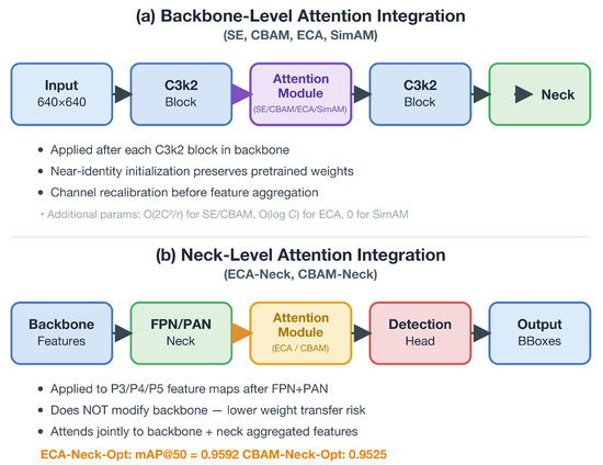
In the ECA-Neck and CBAM-Neck variants, attention modules are applied at the neck output layers rather than inside the backbone. Independent attention masks are computed for each of the P3/8 (layer 16), P4/16 (layer 19) and P5/32 (layer 22) feature maps before they are passed to the detection head. This approach simultaneously evaluates the semantic features produced by the backbone–neck combination without modifying the pretrained backbone weights [37]. The backbone-level and neck-level integration strategies are contrasted in Figure 6.

3.4.7. Hyperparameter Optimization with Optuna TPE

Optuna [18] employs the Tree-structured Parzen Estimator (TPE) [17] algorithm. TPE partitions the past trials into ‘good’ $\left(l\right(x\left)\right)$ and ‘bad’ $\left(g\right(x\left)\right)$ regions and proposes new points that maximize the $l\left(x\right)/g\left(x\right)$ ratio. The objective function (to be minimized) is

$$\theta =-\mathrm{mAP}@50\left(\mathrm{train}(model,D_{train},\theta ),D_{val}\right)$$

(16)

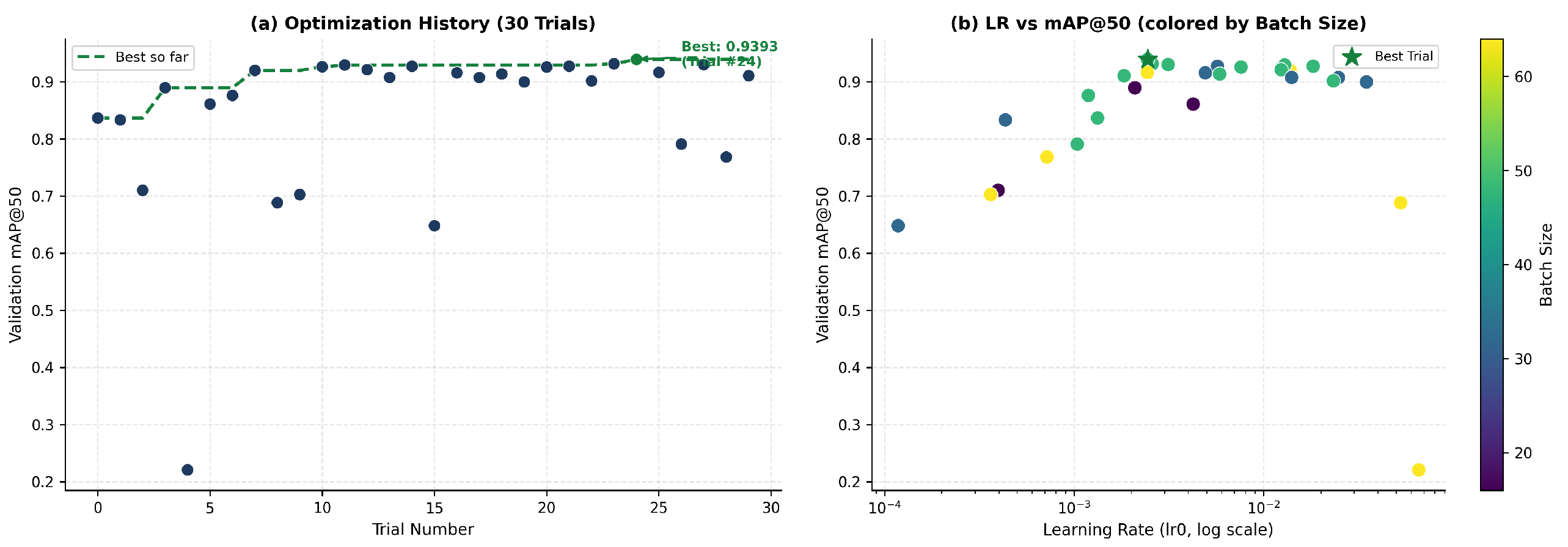
where $\theta$ is the hyperparameter vector, $D_{train}$ is the training set and $D_{val}$ is the validation set. Each trial is evaluated over 20 epochs; the budget is 30 trials (seed = 42). The TPE search was executed once on the baseline architecture, and the single best configuration it returned (trial #24) was then applied uniformly to all optimized variants, rather than being re-optimized separately for each architecture; the selected values are reported in

Table 2. Optuna TPE search space and the single shared configuration (trial #24) applied to all optimized variants, shown alongside the remaining top-five trials of the study. A single study was run on the baseline; no per-architecture re-optimization was performed. Learning rate and weight decay are given in scientific notation.

Parameter	Search Range	Selected (#24)	#23	#27	#11	#21
lr0	Log-U[1 × ${10}^{-4}$, 1 × ${10}^{-1}$]	2.44 × ${10}^{-3}$	2.58 × ${10}^{-3}$	3.13 × ${10}^{-3}$	1.29 × ${10}^{-2}$	1.82 × ${10}^{-2}$
momentum	U[0.70, 0.99]	0.9267	0.917	0.9461	0.8913	0.9136
weight_decay	Log-U[1 × ${10}^{-5}$, 1 × ${10}^{-2}$]	1.96 × ${10}^{-5}$	5.51 × ${10}^{-5}$	1.31 × ${10}^{-4}$	1.15 × ${10}^{-5}$	1.00 × ${10}^{-4}$
batch	{16, 32, 48, 64}	48	48	48	48	48
warmup_epochs	U[1.0, 5.0]	3.6599	3.6641	3.626	3.7568	3.8715
hsv_s	U[0.0, 1.0]	0.4112	0.4883	0.542	0.7078	0.6864
hsv_v	U[0.0, 1.0]	0.6573	0.7426	0.6836	0.9489	0.991
translate	U[0.0, 0.2]	0.1381	0.1427	0.1885	0.1165	0.1269
scale	U[0.0, 0.9]	0.0844	0.0051	0.2646	0.0067	0.0181
fliplr	U[0.0, 1.0]	0.0688	0.2044	0.082	0.0188	0.0134
mixup	U[0.0, 0.3]	0.1306	0.1238	0.2182	0.1574	0.1676
copy_paste	U[0.0, 0.3]	0.1223	0.1231	0.2149	0.07	0.0873
label_smoothing	U[0.0, 0.1]	0.0429	0.0449	0.0533	0.0446	0.0449

, together with the remaining top-five trials.

Table 3. Standard training hyperparameter set used by all model variants.

Hyperparameter	Value
Image size	640 × 640 px
Batch size	32
Epochs	100 (patience = 10)
Optimizer	AdamW
Initial learning rate (lr0)	0.01
Momentum (${\beta }_1$)	0.937
Weight decay	5 × ${10}^{-4}$
Warmup epochs	3
Box loss gain	7.5
Classification loss gain	0.5
DFL loss gain	1.5
Mosaic augmentation	1.0
HSV-Saturation	0.7
HSV-Value	0.4
Horizontal flip	0.5
Mixed precision	FP16

summarizes the baseline hyperparameter set used in the ablation study. The Optuna search space is summarized in Table 1. The optimization hyperparameters and data-augmentation strategies that are typically used during deep-learning training are sampled from a wide range. Continuous-scale parameters such as the learning rate (lr0) and weight decay are sampled from log-uniform distributions, defining a broad search space that promotes generalization. Discrete hyperparameters such as the batch size are optimized over a limited set to balance computational efficiency and training stability. Label smoothing is added as a regularization mechanism that discourages overconfident predictions and thereby improves generalization.

3.4.8. Experimental Setup

To ensure reproducibility, a common training configuration was used for all variants. Training was performed on an NVIDIA GPU with FP16 mixed precision; a patience = 10 early-stopping criterion was enforced with a 100-epoch hard limit.

4. Experimental Results

4.1. Ablation Study Under Standard Conditions

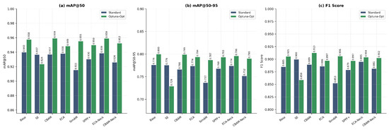
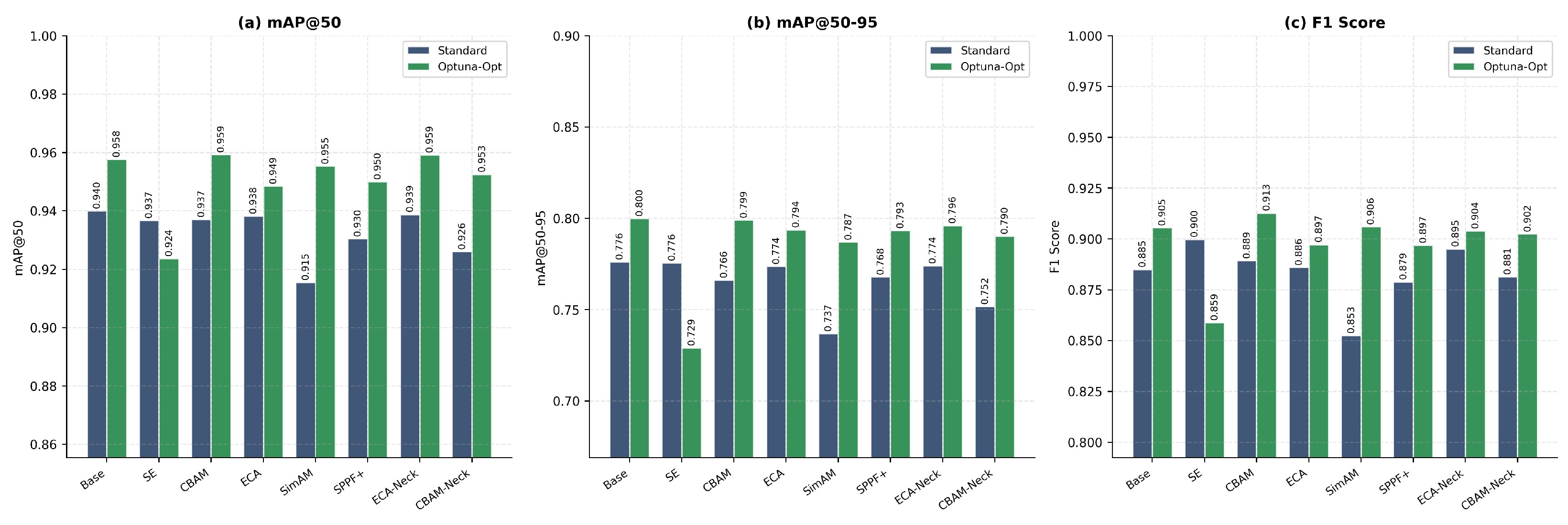
Figure 7 reports the ablation graphs that compare the standard and Optuna-optimized models on three principal metrics. Under standard conditions, all attention mechanisms produce mAP@50 values close to one another (0.9155–0.9388); the baseline model reaches the highest value at 0.9400. After optimization, CBAM-Opt (0.9593) and ECA-Neck-Opt (0.9592) attain the strongest peak performance. Detailed metrics are tabulated in

Table 4. Validation metrics under standard hyperparameters (green-shaded cells mark the highest value per metric).

Model	mAP@50	mAP@50–95	Precision	Recall	F1
Base	0.9400	0.7762	0.8766	0.9008	0.8851
SE	0.9367	0.7756	0.9185	0.8846	0.8999
CBAM	0.9371	0.7663	0.9204	0.8718	0.8893
ECA	0.9383	0.7738	0.8817	0.8944	0.8860
SimAM	0.9155	0.7370	0.8620	0.8549	0.8525
SPPF+	0.9305	0.7679	0.9004	0.8659	0.8789
ECA-Neck	0.9388	0.7741	0.9021	0.8919	0.8952
CBAM-Neck	0.9260	0.7518	0.8784	0.8784	0.8815

.

As observed in Table 4, the baseline model (Base) achieves the highest mAP@50 (0.9400), while attention-based models deliver substantial improvements on the precision and F1-score metrics. SE and CBAM stand out for high precision values but exhibit partial drops in recall. ECA-based approaches strike a more balanced compromise between precision and recall, preserving overall stability. SimAM produces the lowest values on every metric, indicating that this approach is not optimally aligned with the current architecture. When neck-level attention integration is examined, ECA-Neck delivers stronger results than backbone-level attention applications on both mAP@50–95 and F1-score, demonstrating that attention modules influence not only model behavior in general but also that the performance gain depends on the integration position within the architecture.

4.2. Performance of Optuna-Optimized Models

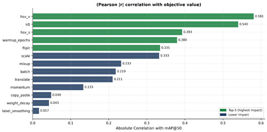
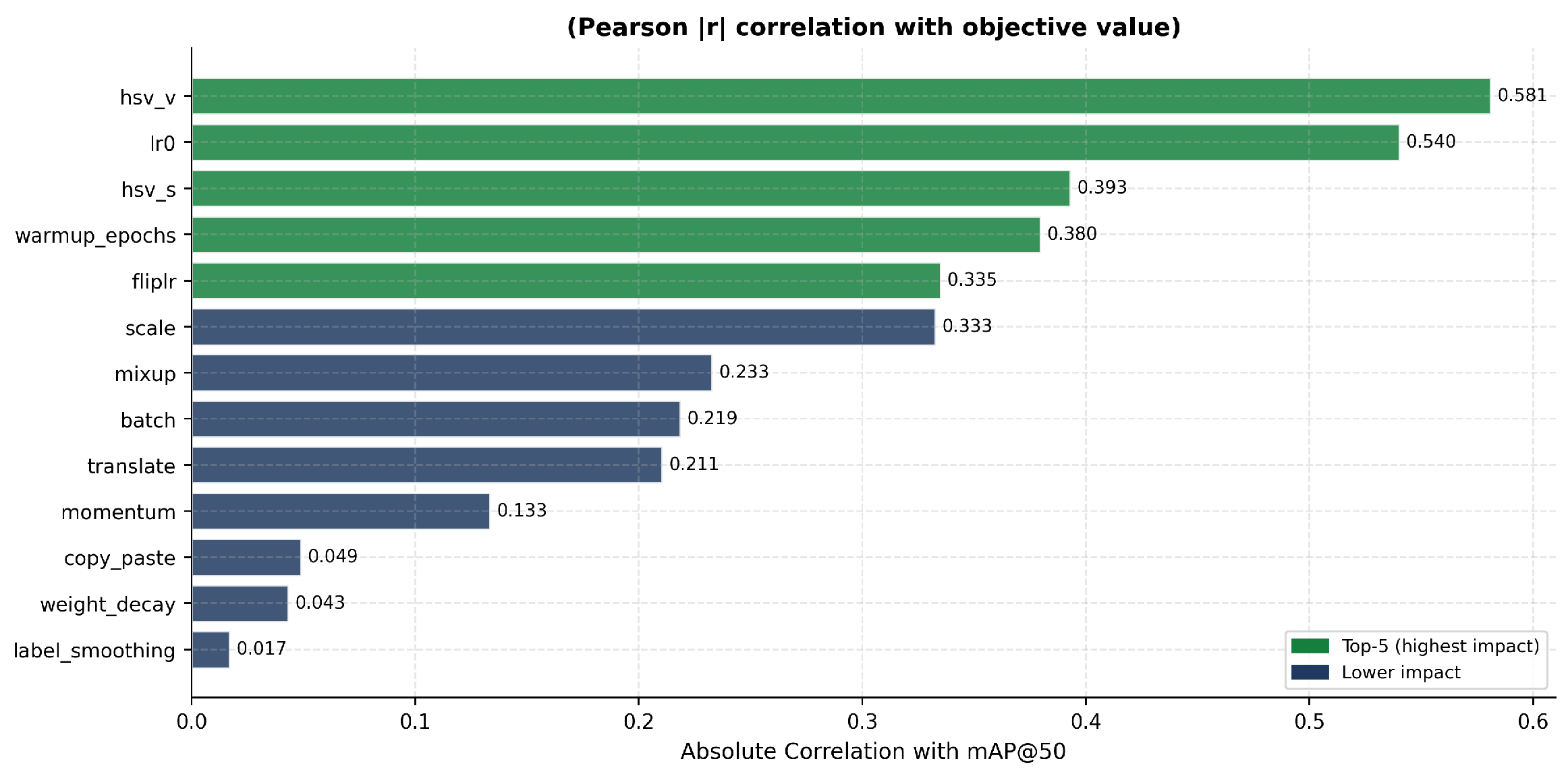
Figure 8 visualizes the Optuna optimization process. As shown in Figure 8a, validation mAP@50 improves rapidly during early trials and stabilizes near 0.92 in later trials. Figure 8b shows that intermediate learning rates yield the highest mAP@50, while excessively low or high learning rates degrade performance. The hyperparameter importance analysis in Figure 9 indicates that HSV-V (0.581), lr0 (0.540) and HSV-S (0.393) are the three most influential factors. Detailed metric values are reported in

Table 5. Validation metrics of Optuna-optimized variants ($\Delta$mAP@50 relative to standard). Green-shaded cells mark the highest value in each column; the red-shaded cell marks the only negative $\Delta$mAP@50.

Model	mAP@50	mAP@50–95	Precision	Recall	F1	$\mathbf{\Delta }$mAP@50
Base-Opt	0.9576	0.8000	0.9221	0.8933	0.9055	+0.0176
SE-Opt	0.9237	0.7291	0.8802	0.8441	0.8589	−0.0130
CBAM-Opt	0.9593	0.7991	0.9288	0.9002	0.9128	+0.0222
ECA-Opt	0.9485	0.7938	0.8886	0.9095	0.8973	+0.0102
SimAM-Opt	0.9553	0.7870	0.9187	0.8987	0.9061	+0.0398
SPPF+-Opt	0.9500	0.7933	0.9146	0.8830	0.8970	+0.0195
ECA-Neck-Opt	0.9592	0.7961	0.9177	0.8941	0.9040	+0.0204
CBAM-Neck-Opt	0.9525	0.7902	0.9094	0.8984	0.9025	+0.0265

.

As shown in Table 5, Optuna-optimized configurations deliver consistent performance gains in almost every architecture. The Base-Opt model improves the baseline mAP@50 from 0.9400 to 0.9576 ($\Delta$ = +0.0176). The highest mAP@50 value, 0.9593, is obtained by CBAM-Opt, which also leads in the F1-score with 0.9128. It should be emphasized, however, that the margin separating the top optimized configurations is very small (on the order of 0.001–0.01 mAP@50) and should be interpreted with caution rather than as evidence of a decisive advantage of any single module. As shown by the repeated-seed analysis in Section 4.12 and

Table 6. Repeated-seed statistical validation of the optimized models (seeds 0, 1, 2, 3, 42): mean ± standard deviation and 95% confidence interval over five independent runs. Italic subheadings separate the validation and test blocks.

Model	mAP@50 (Mean ± SD)	mAP@50 95% CI	mAP@50–95	Precision	Recall	F1
val split
Base-Opt	0.9527 ± 0.0084	[0.9423, 0.9631]	0.7900 ± 0.0158	0.9180	0.8912	0.9020
SE-Opt	0.9455 ± 0.0127	[0.9297, 0.9613]	0.7778 ± 0.0293	0.9043	0.8840	0.8915
CBAM-Opt	0.9522 ± 0.0109	[0.9387, 0.9657]	0.7899 ± 0.0193	0.9080	0.9007	0.9021
ECA-Neck-Opt	0.9555 ± 0.0051	[0.9491, 0.9618]	0.7888 ± 0.0141	0.9113	0.9119	0.9098
SimAM-Opt	0.9429 ± 0.0144	[0.9250, 0.9608]	0.7689 ± 0.0224	0.9114	0.8895	0.8973
test split
Base-Opt	0.9208 ± 0.0116	[0.9064, 0.9352]	0.7552 ± 0.0175	0.8757	0.8970	0.8850
SE-Opt	0.9195 ± 0.0104	[0.9065, 0.9325]	0.7460 ± 0.0243	0.8717	0.8955	0.8820
CBAM-Opt	0.9264 ± 0.0120	[0.9115, 0.9413]	0.7598 ± 0.0228	0.8827	0.9019	0.8904
ECA-Neck-Opt	0.9283 ± 0.0170	[0.9072, 0.9494]	0.7585 ± 0.0240	0.8814	0.9018	0.8902
SimAM-Opt	0.9169 ± 0.0169	[0.8959, 0.9378]	0.7466 ± 0.0295	0.8661	0.9014	0.8823

and

Table 7. Paired significance tests between the top optimized configurations. The paired t-test is the primary test; because the exact two-sided Wilcoxon signed-rank test cannot fall below $p=0.0625$ at $n=5$, it is reported as a direction-consistency check.

Split	Metric	Comparison	Mean Diff.	t	p (t)	Sig.	p (W)
val	mAP@50	CBAM-Opt vs. ECA-Neck-Opt	−0.0033	−0.666	0.5417	no	1.0
val	mAP@50–95	CBAM-Opt vs. ECA-Neck-Opt	+0.0010	0.101	0.9242	no	1.0
val	mAP@50	CBAM-Opt vs. Base-Opt	−0.0005	−0.086	0.9355	no	1.0
val	mAP@50–95	CBAM-Opt vs. Base-Opt	−0.0002	−0.015	0.9888	no	1.0
val	mAP@50	CBAM-Opt vs. SE-Opt	+0.0067	0.785	0.4765	no	0.625
val	mAP@50–95	CBAM-Opt vs. SE-Opt	+0.0120	0.668	0.5408	no	1.0
test	mAP@50	CBAM-Opt vs. ECA-Neck-Opt	−0.0019	−0.238	0.8232	no	0.625
test	mAP@50–95	CBAM-Opt vs. ECA-Neck-Opt	+0.0012	0.109	0.9182	no	0.8125
test	mAP@50	CBAM-Opt vs. Base-Opt	+0.0056	0.645	0.5538	no	0.4375
test	mAP@50–95	CBAM-Opt vs. Base-Opt	+0.0046	0.291	0.7858	no	0.625
test	mAP@50	CBAM-Opt vs. SE-Opt	+0.0069	0.955	0.3939	no	0.4375
test	mAP@50–95	CBAM-Opt vs. SE-Opt	+0.0137	0.809	0.4638	no	0.4375

, none of these differences is statistically significant, and the seed-averaged ranking differs from the single-run ordering reported here. ECA-Neck-Opt produces a comparably strong performance of 0.9592, confirming that neck-level attention integration is highly effective in optimized settings. SimAM provides the largest absolute gain after optimization ($\Delta$mAP@50 = +0.0398). In contrast, SE is the only architecture that suffers a post-optimization drop, indicating that the benefit of attention mechanisms varies with the specific module–optimizer interaction.

4.3. Training Convergence Behavior

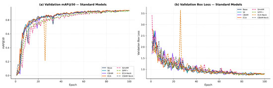
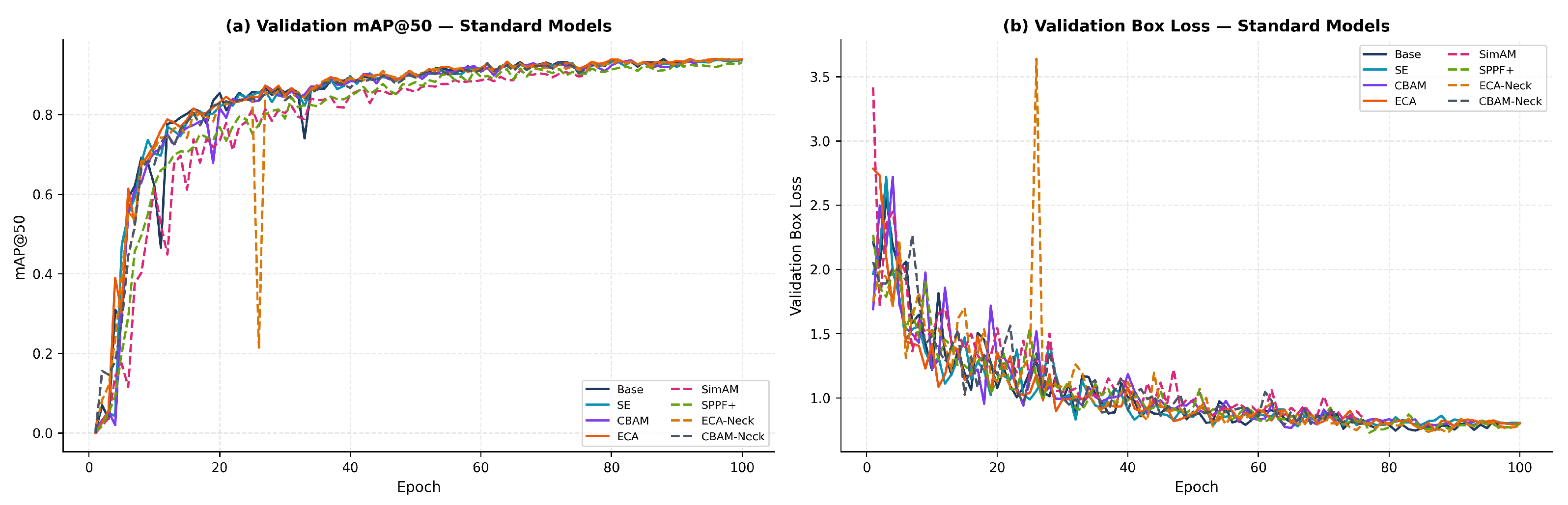
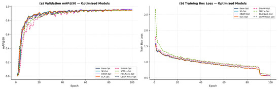
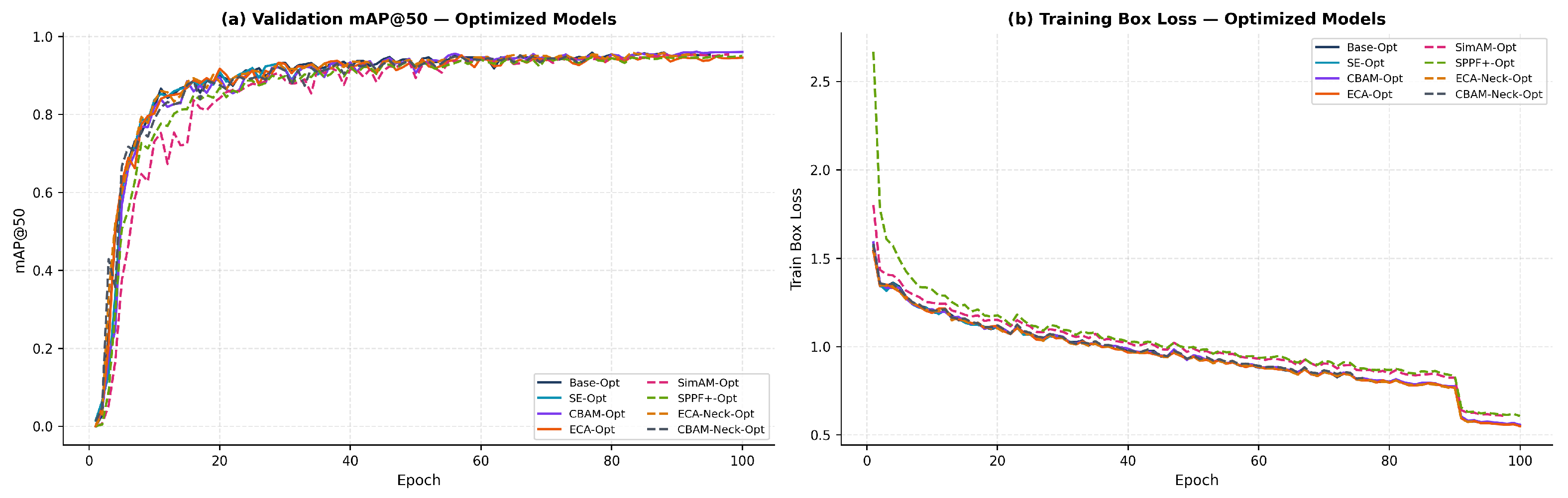
Figure 10 and Figure 11 show the per-epoch validation mAP@50 and loss curves for all models. Under standard conditions, shown in Figure 10, the Base and ECA models converge earliest and most steadily. SimAM displays a slower and more oscillatory convergence in the standard configuration, which can be attributed to the sensitivity of the analytical-attention strategy to the default data-augmentation configuration. Once optimized, as shown in Figure 11, all models converge faster and reach a higher performance plateau.

4.4. Architecture-Specific Optimization Gain

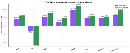
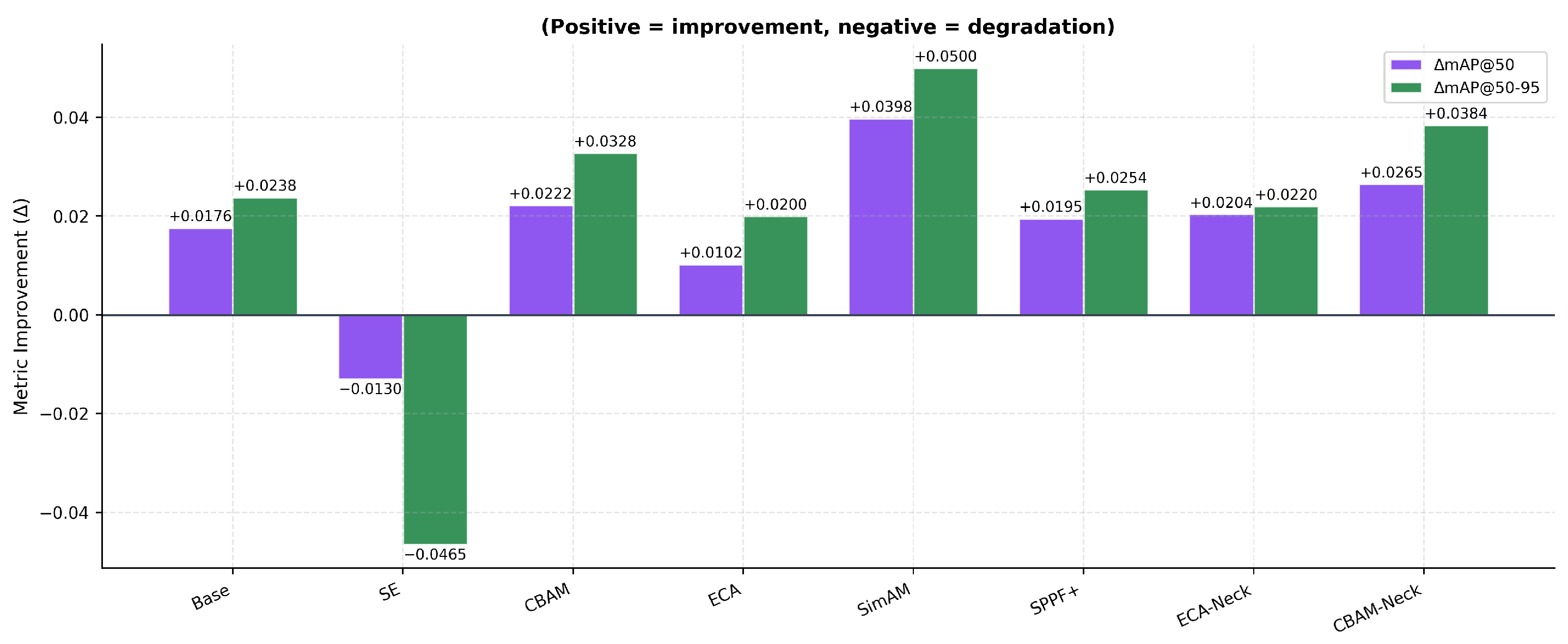
Figure 12 displays the per-architecture Optuna optimization gain ($\Delta$mAP@50 and $\Delta$mAP@50–95). SimAM exhibits the largest absolute improvement on both metrics. CBAM and CBAM-Neck achieve strong absolute gains; conversely, the SE variant suffers a $-0.013$ mAP@50 loss, the only negative change observed.

4.5. Precision and Recall Comparison

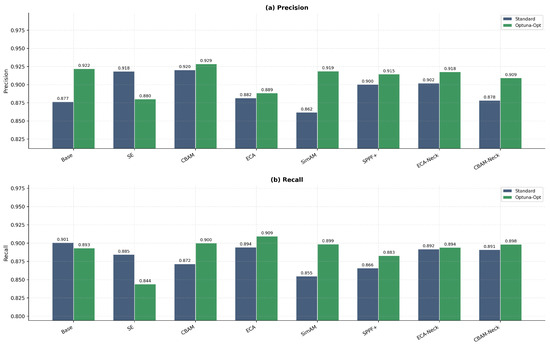
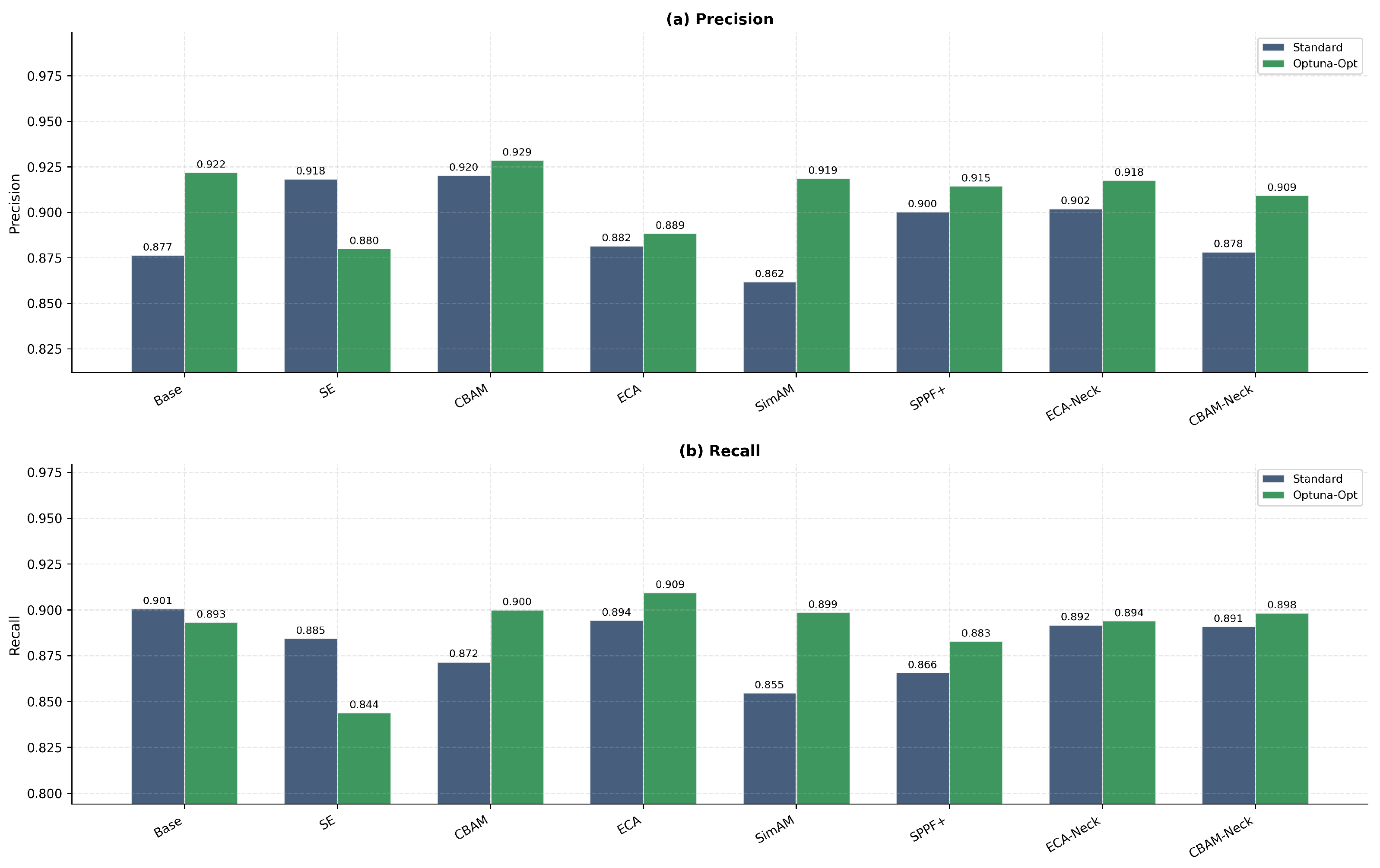
Figure 13 compares the precision and recall values of every model variant. Under standard conditions, SE and CBAM produce high precision (>0.918), while ECA-Opt attains the highest recall (0.9095), with ECA-Neck-Opt close behind (0.8941). CBAM-Opt achieves the most balanced and highest values on both metrics (precision = 0.9288, recall = 0.9002).

4.6. Multi-Metric Profile (Radar) and Improvement Heatmap

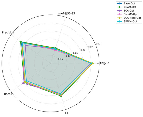
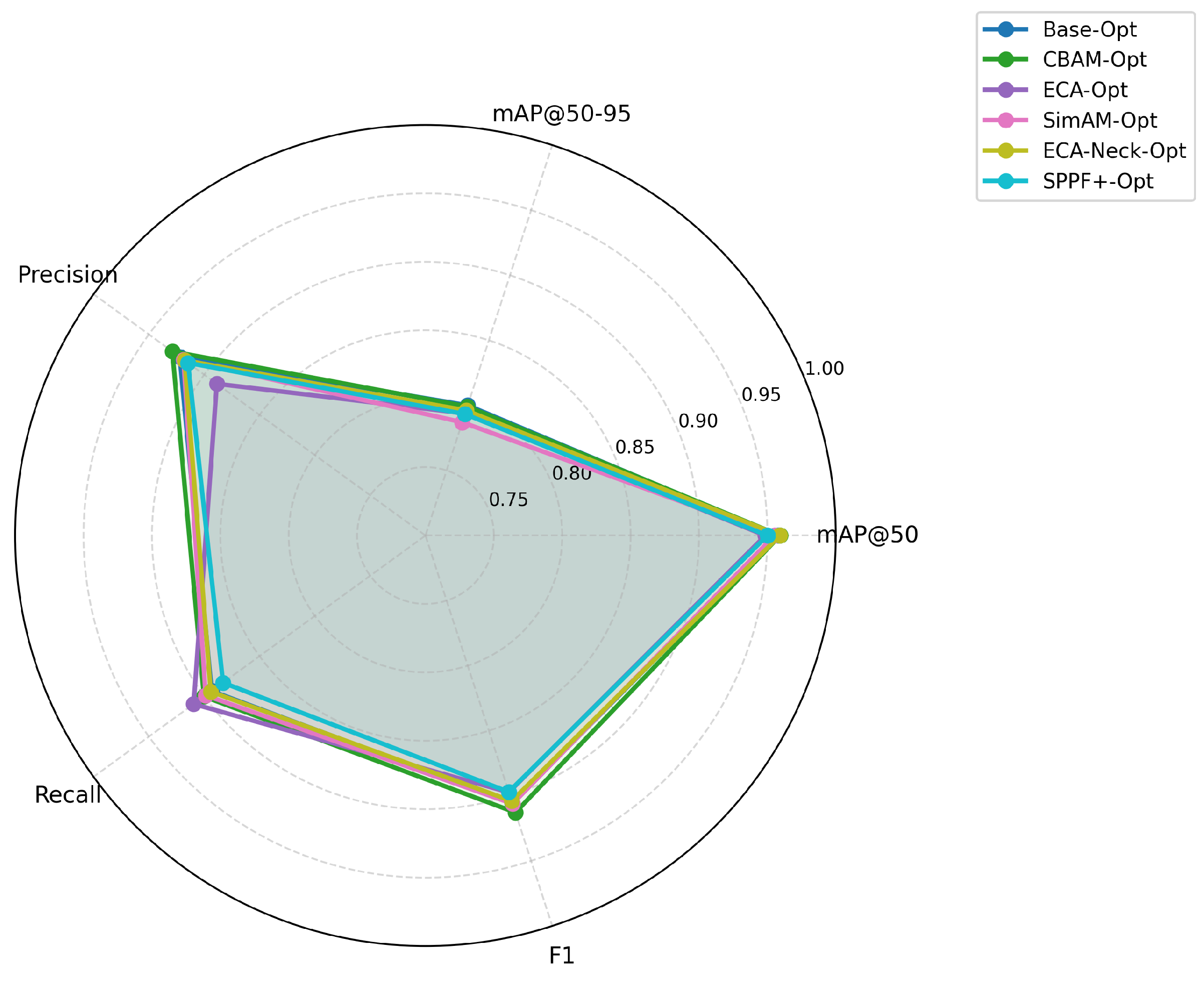
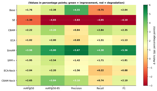
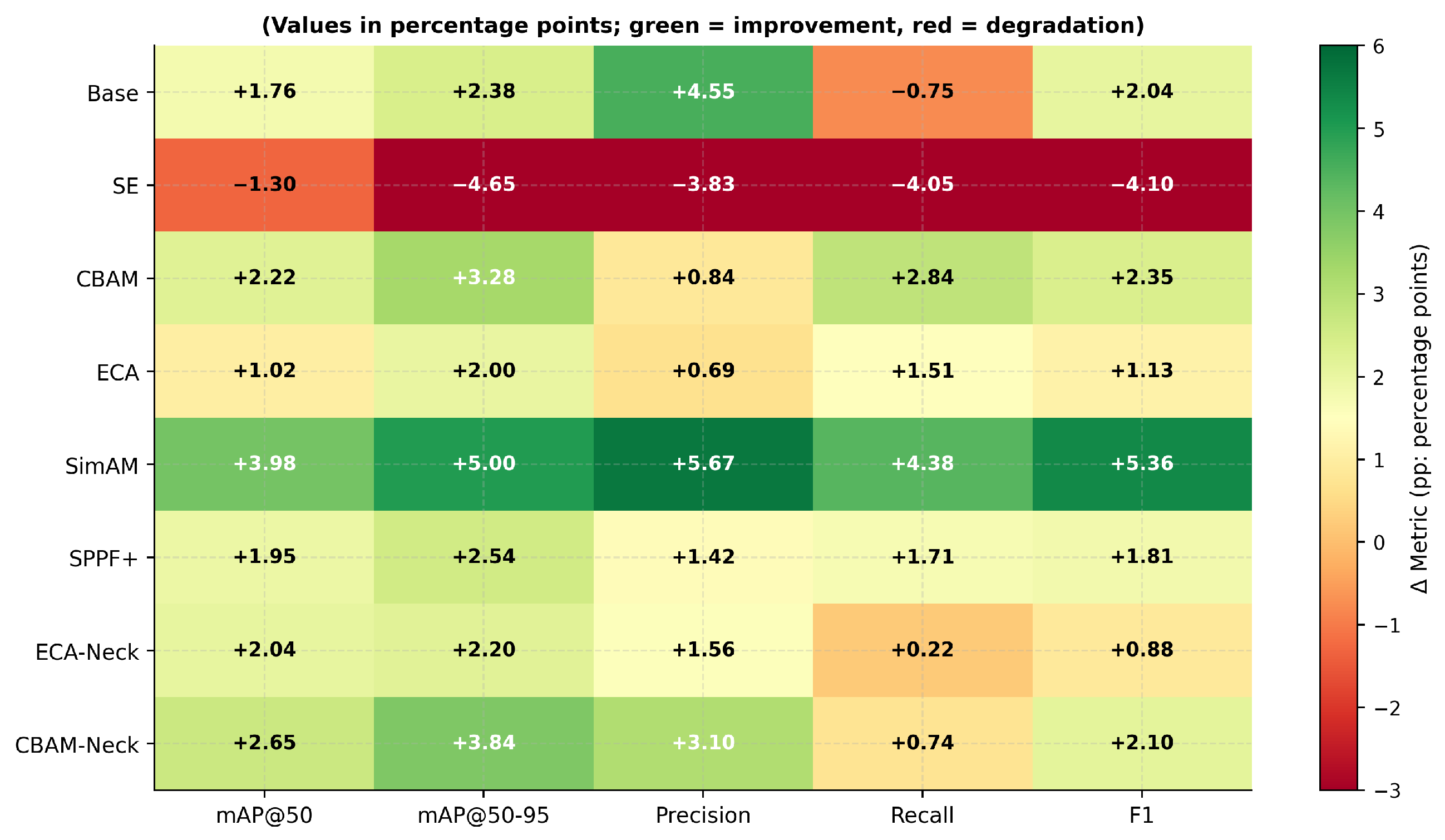
Figure 14 presents the multi-metric radar comparison of the optimized variants over five dimensions. CBAM-Opt and ECA-Neck-Opt cover the largest radar area, while SE-Opt occupies the smallest. Figure 15 displays the metric-improvement heatmap of Optuna optimization (percentage-point change relative to the standard counterpart). SimAM provides the most consistent improvement across all metrics (+3.98, +5.00, +5.67, +4.38 and +5.36 percentage points, respectively, on mAP@50, mAP@50–95, precision, recall and F1). The SE variant exhibits negative changes on every metric.

4.7. Class-Level Confusion and Precision–Recall Analysis

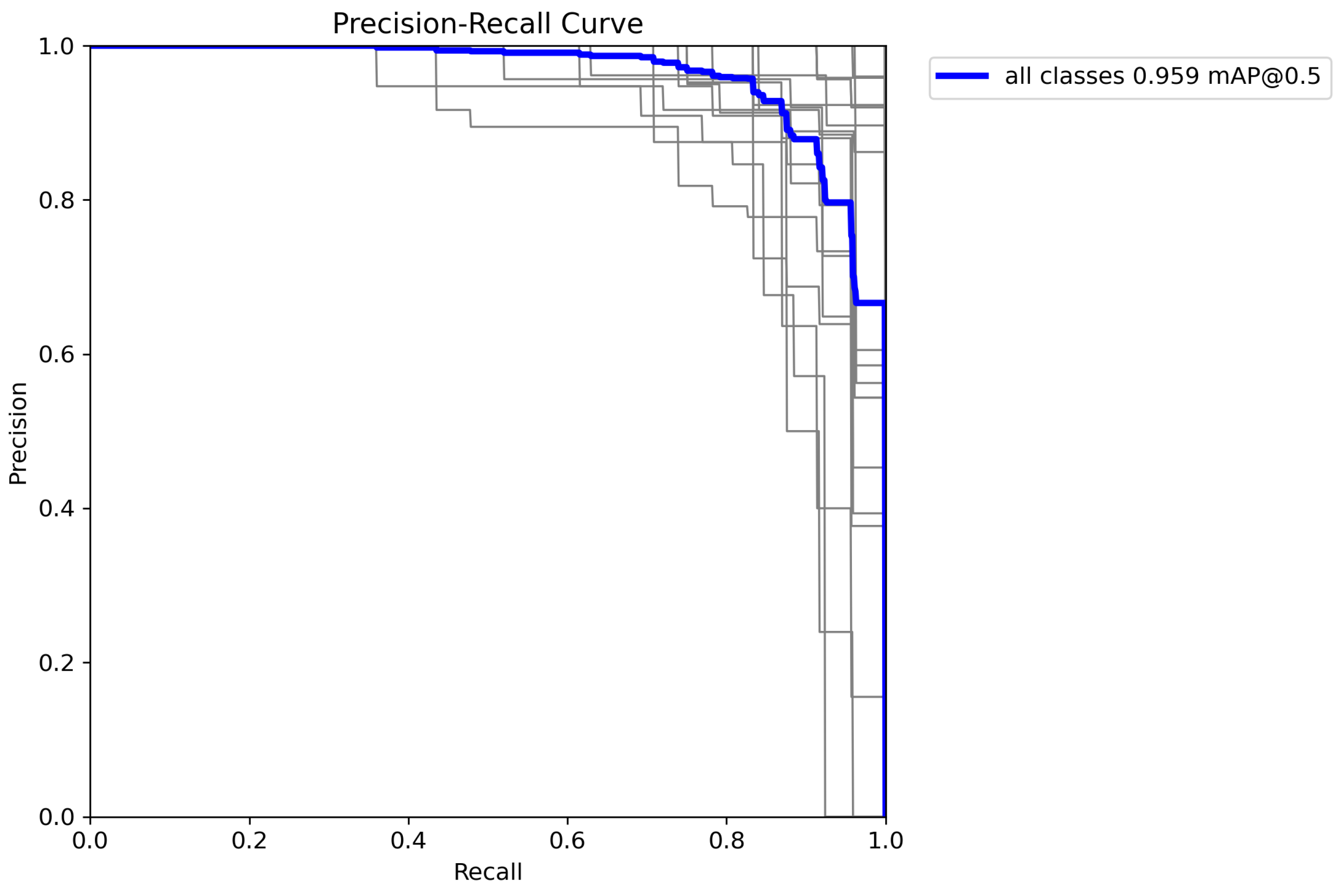
The normalized confusion matrix of the best-performing CBAM-Opt model is given in Figure 3. Most classes (AnArFo, CuGuSc, MaAnCaFo, and WiOrCu) are recognized with 96–100% accuracy. Cross-class confusion is observed mainly in the visually similar MaLoInFo, OrLiCu and StArFo categories. Figure 16 shows the corresponding per-class precision–recall curves; the aggregate mAP@0.5 = 0.9593 across all classes confirms the strong generalization of the model.

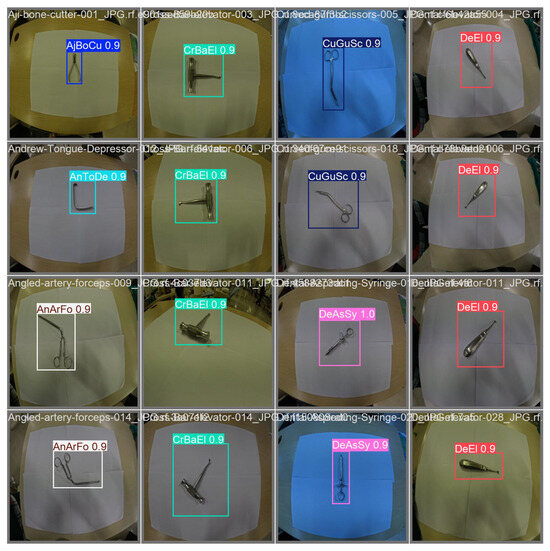
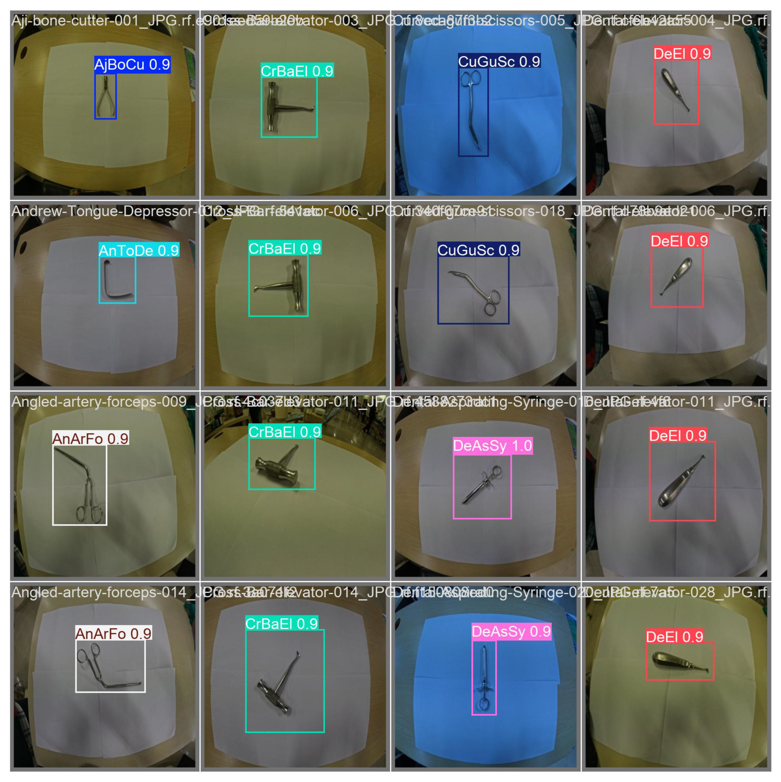
Sample prediction results of the object-detection model trained on the surgical instrument dataset using the CBAM-Opt model are shown in Figure 17.

Figure 17 presents sample prediction results of the object detection model using the CBAM-Opt model on a surgical instrument dataset. The CBAM-Opt model correctly identified different classes of surgical instruments with high confidence scores (0.9–1.0) and successfully localized the relevant objects within the image. The results show that the classification and positioning performance of the model is stable under different background conditions, viewing angles, and instrument positions. The fact that the bounding boxes largely overlap with the object boundaries reveals that the model can effectively learn visual features. These findings demonstrate that the developed approach exhibits a level of performance suitable for applications involving the automatic recognition and real-time tracking of surgical instruments.

4.8. Computational Complexity Analysis

Table 8. Computational cost of each attention configuration. C denotes the channel count at the integration point, and r is the reduction ratio; the percentage columns express the extra cost relative to the Base YOLOv26n model (2.60M parameters/8.2 GFLOPs).

Configuration	Extra Parameters (Theoretical, Per Block)	Extra Parameters (% of Base)	Extra FLOPs (% of Base)	Note
Base (YOLOv26n)	—(reference: 2.60M total params)	—(8.2 GFLOPs total)	—	Reference baseline (no attention)
+ SE ($r=16$)	$O(2C^2/r)$	∼+1.0%	∼+1.0%	Channel-only re-weighting
+ CBAM ($r=16$)	$O(2C^2/r+49)$	∼+1.5%	∼+1.5%	Channel + 7 × 7 spatial mask
+ ECA	$O(k·C)$, $k={log}_2\left(C\right)$	<+0.5%	∼+0.5%	1D conv; no dim. reduction
+ SimAM	0 (parameter-free)	0	∼0%	Analytical 3D attention
+ SPPF+	≈150 K (three pool branches)	∼+5.8%	∼+5.0%	Multi-kernel SPPF (k = 3,5,7)
+ ECA-Neck (3 scales)	$O(3k·C)$	<+0.5%	∼+1.0%	Applied at P3/P4/P5 of neck
+ CBAM-Neck (3 scales)	$O\left(3(2C^2/r+49)\right)$	∼+1.5%	∼+1.5%	Applied at P3/P4/P5 of neck

summarizes, for each attention configuration, both the theoretical per-block parameter cost (asymptotic big-O form) and the practical impact on the YOLOv26n baseline (percentage of extra parameters and FLOPs relative to the 2.60 M parameter/8.2 GFLOPs baseline). SimAM is the only attention module that introduces zero additional learnable parameters. SPPF+ produces the largest cost increment (∼+5% FLOPs, ∼150 K extra parameters) because of its three parallel pooling branches, yet this still represents only a small fraction of the total YOLOv26n compute budget.

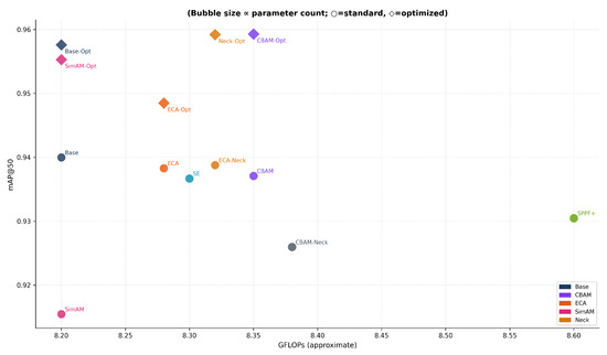
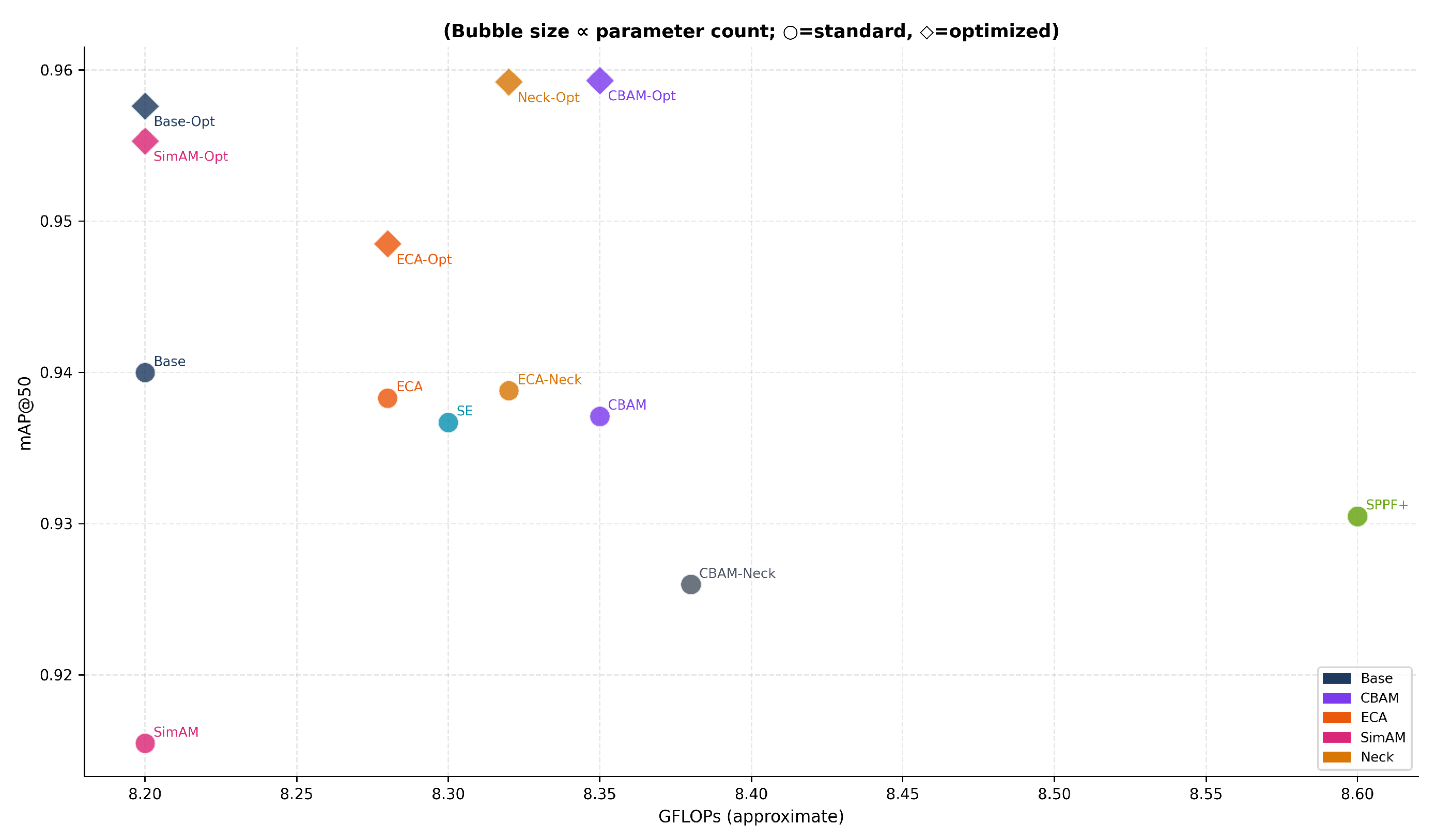
Figure 18 visualizes the accuracy–efficiency trade-off. All attention modules deliver meaningful mAP improvements with negligible (<5%) FLOPs overhead, demonstrating that attention modules are computationally efficient modifications that are practical even on hardware-constrained clinical systems.

4.9. Inference Speed Analysis

Inference latency on a single NVIDIA GPU under FP16 is reported in

Table 9. Inference speed comparison (NVIDIA GPU, FP16; approximate values).

Model	Preprocess (ms)	Inference (ms)	Postprocess (ms)
Base	3.1	7.6	2.7
SE	3.1	7.7	2.7
CBAM	3.2	7.8	2.8
ECA	3.1	7.7	2.7
SimAM	3.1	7.6	2.7
SPPF+	3.2	8.1	2.8
ECA-Neck	3.1	7.8	2.7
CBAM-Neck	3.2	7.9	2.8

. Preprocessing times remain constant at ∼3.1–3.2 ms, post-processing varies between 2.7 and 2.8 ms, and inference latency varies between 7.6 and 8.1 ms across models. The Base and SimAM variants share the lowest inference time (7.6 ms); SPPF+ has the highest latency (8.1 ms). Inference-time increases due to attention modules are within acceptable limits for real-time use.

4.10. Training-Time Overhead

Table 10. Estimated training time and attention module overhead.

Model	Epoch (s, est.)	Total (Min)	Overhead	Note
Base	∼3.5	∼210	—	Reference
SE	∼3.6	∼216	+∼3%	Channel attention
CBAM	∼3.7	∼222	+∼6%	Channel + spatial
ECA	∼3.6	∼216	+∼3%	1D conv
SimAM	∼3.5	∼210	∼0	Parameter-free
SPPF+	∼3.8	∼228	+∼9%	3-stream pooling
ECA-Neck	∼3.7	∼222	+∼6%	3-scale ECA
CBAM-Neck	∼3.8	∼228	+∼9%	3-scale CBAM
Base-Opt	∼3.5	∼210	+Opt: 8–10 s × 30	Single Optuna study (baseline)
CBAM-Opt	∼3.7	∼222	—	Retrained with shared best config

reports the approximate training time per epoch and per full run, together with the attention module overhead. The per-epoch overhead is between 0% and 9% and remains negligible under even tight hardware budgets. The Optuna optimization run requires an additional 10–15 h (30 trials ×∼20 epochs) and was performed once on the baseline architecture; this is a one-time investment that must be weighed against the performance gain (average +0.015 to +0.040 mAP@50) when selecting an architecture for production.

4.11. Quantitative Comparison with Recent Surgical/Dental Detection Work

Table 11. Quantitative comparison with selected literature (bold, green-shaded rows denote this work).

Study	Year	Model	Attention	HPO	Data	mAP@50/ mAP@50–95	Note
Redmon et al. [1]	2016	YOLO	—	—	General	—	Slow training
Liu et al. [25]	2024	YOLOv7-Rep	—	—	Laparoscopic	—	Embedded
Jiang et al. [23]	2023	YOLOv5+	Custom	—	Laparoscopic	∼0.91 AP/—	Few classes
Ran et al. [24]	2023	YOLOv7x	Custom	—	Laparoscopic	∼0.89 mAP/—	Embedded focus
Chien et al. [13]	2024	YOLOv8-AM	CBAM/ECA	—	X-ray	0.94+ /—	Single attention
Wang et al. [22]	2021	YOLOv4	—	—	Surgical	∼0.88/—	Older architecture
Poomrittigul [6]	2026	YOLOv8	—	—	Dental	—/—	First dental YOLO
This work (CBAM-Opt)	2026	YOLOv26n	SE + CBAM + ECA + SimAM + Neck	Optuna-TPE	Dental (22 cls.)	0.9593/0.7991	Highest mAP@50
This work (Base-Opt)	2026	YOLOv26n	—	Optuna-TPE	Dental (22 cls.)	0.9576/0.8000	Highest mAP@50–95

places the best results of this work next to recent surgical and dental detection studies. Two cells highlight the configurations introduced by the present paper: CBAM-Opt yields the highest mAP@50 (0.9593), and Base-Opt yields the highest mAP@50–95 (0.8000). Note that direct comparison must be interpreted carefully because the underlying datasets (laparoscopic, X-ray, and dental panoramic) differ in image modality and class count.

4.12. Statistical Robustness Analysis

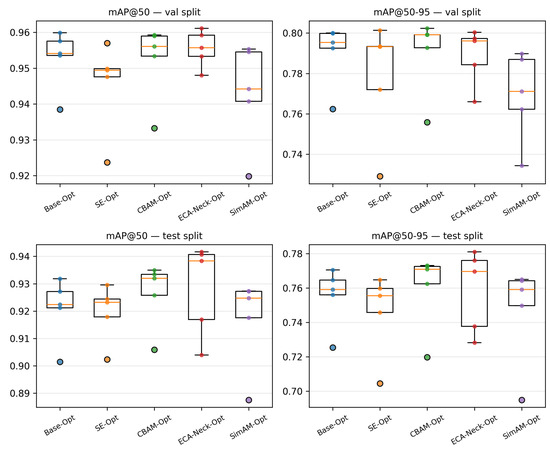
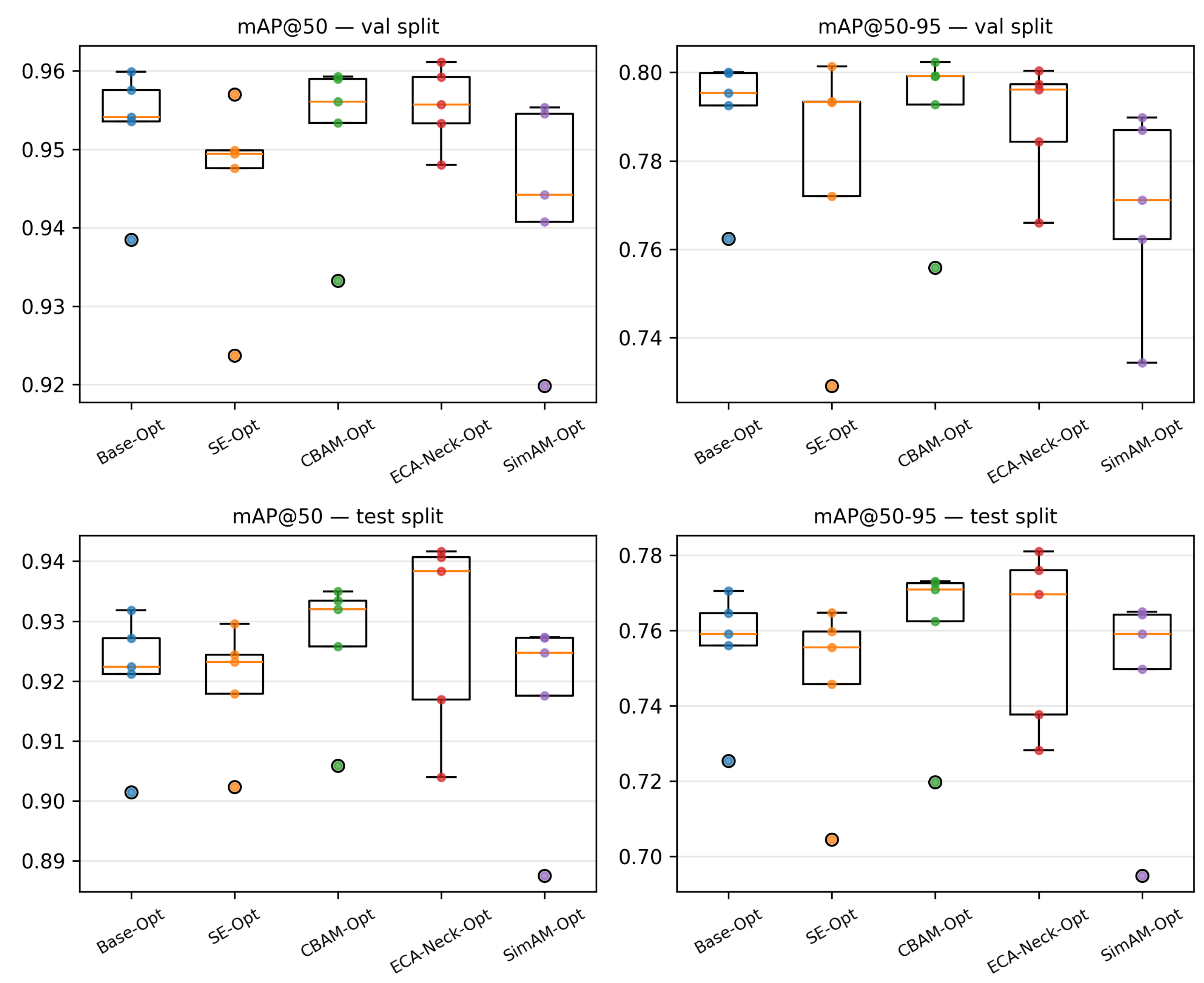
To assess whether the differences among the top optimized configurations are systematic rather than artifacts of a single training run, the five key optimized configurations (Base-Opt, SE-Opt, CBAM-Opt, ECA-Neck-Opt and SimAM-Opt) were each retrained with five random seeds ($s\in \{0,1,2,3,42\}$), keeping the shared Optuna-selected hyperparameters listed in Table 2 and the train/validation/test partition fixed so that only weight initialization and data shuffling varied across runs. All runs used the same software stack (Ultralytics 8.4.47, PyTorch 2.7.1+cu118, Python 3.12.8) on a single NVIDIA Quadro P5000 (16 GB). Table 6 reports the mean ± standard deviation and the 95% confidence interval (Student’s t, $n=5$) for every metric on both the validation and test splits, and Table 7 reports paired t-tests and Wilcoxon signed-rank tests between the top model pairs. Figure 19 visualizes the seed-level distributions.

The analysis shows that none of the differences between the top configurations is statistically significant. On validation mAP@50, the paired t-test yields $p=0.5417$ for CBAM-Opt vs. ECA-Neck-Opt (mean difference $-0.0033$), $p=0.9355$ for CBAM-Opt vs. Base-Opt ($-0.0005$), and $p=0.4765$ for CBAM-Opt vs. SE-Opt ($+0.0067$); the Wilcoxon test agrees in direction in every case. The five-seed means further show that the single-run ranking is not stable: averaged over seeds, ECA-Neck-Opt attains the highest validation mAP@50 ($0.9555\pm 0.0051$), marginally above CBAM-Opt ($0.9522\pm 0.0109$) and Base-Opt ($0.9527\pm 0.0084$), whereas the single-run values in Table 5 place CBAM-Opt first. This confirms the Reviewers’ concern that sub-0.01 mAP@50 gaps must not be over-interpreted, and it is the empirical basis for the moderated wording adopted in Sections 4.2 and the Conclusions. SE-Opt retains the lowest mean on both splits, so its relative degradation is consistent across seeds rather than a single-run artifact.

4.13. Data-Leakage Audit and Group-Disjoint Split Evaluation

Because the dataset is a Roboflow export, every filename encodes the identity of its source image, which allows source-image groups (an original photograph together with all of its augmented copies) to be reconstructed exactly. A programmatic audit of all 2178 images/831 source-image groups found that 0 of 831 groups span more than one split: no augmented copy of any training image appears in the validation or test sets, and the evaluation splits consist exclusively of single-copy groups. Random image-level splitting, therefore, did not introduce near-duplicate leakage in this dataset.

Although no leakage exists, the original split allocates 93.0% of the images to training (2025/73/80 images), leaving small evaluation sets. To verify that the reported performance does not depend on this particular partition, a group-disjoint, class-stratified 70/20/10 re-split was constructed (578/169/84 source-image groups; 1509/169/84 images, with the evaluation splits restricted to one representative copy per group), and Base-Opt and CBAM-Opt were retrained from scratch on it using the same shared configuration.

Table 12. Original random split vs. group-disjoint, class-stratified 70/20/10 re-split. Base-Opt and CBAM-Opt were retrained from scratch on the re-split. Precision/Recall cells show original/group-disjoint values.

Model	Split	mAP@50 Orig.	mAP@50 Group	mAP@50–95 Orig.	mAP@50–95 Group	P (Orig/Grp)	R (Orig/Grp)
Base-Opt	val	0.9576	0.8865	0.8000	0.6892	0.9221/0.8526	0.8933/0.8421
Base-Opt	test	0.9224	0.9312	0.7591	0.7271	0.8679/0.8426	0.9093/0.8952
CBAM-Opt	val	0.9593	0.8936	0.7991	0.7100	0.9288/0.8611	0.9002/0.8537
CBAM-Opt	test	0.9350	0.9593	0.7731	0.7643	0.8921/0.9200	0.9191/0.9064

compares both partitions. Performance is preserved under the stricter partition: CBAM-Opt reaches a test mAP@50 of 0.9593 (versus 0.9350 on the original test split) and Base-Opt 0.9312 (versus 0.9224), supporting the robustness claimed in the title. The lower group-disjoint validation figures reflect the small, single-copy validation set rather than a drop in generalization, as the independent test split confirms.

5. Discussion

5.1. Comparative Analysis of Attention Mechanisms

The standard-condition ablation shows that the absolute mAP@50 effect of attention mechanisms is comparatively modest (<0.025), while the precision gain is pronounced. SE (precision = 0.9185) and CBAM (precision = 0.9204) substantially exceed the baseline (0.8766). This finding agrees with the literature [9,10] documenting that channel-attention mechanisms reduce spurious detections by emphasizing object features over background responses. ECA and ECA-Neck deliver recall-oriented profiles (recall $>0.89$), suggesting that local channel interaction without dimensionality reduction reduces the likelihood of missing visually similar dental instruments—a property that is clinically critical for `zero-miss’ safety requirements in dental and other surgical applications.

5.2. SimAM Anomaly and Hyperparameter Dependence

SimAM’s low standard-condition performance (mAP@50 = 0.9155) suggests that the parameter-free analytical-attention approach may exhibit insufficient capacity on small datasets. Because no parameters are learned, the effectiveness of SimAM is entirely tied to the training environment formed by the data augmentation, learning rate and batch size. Under the shared Optuna-selected configuration reported in Table 2 (momentum = 0.9267; initial learning rate = 2.44 × ${10}^{-3}$), the reduced learning rate relative to the standard setting (0.01) appears to suppress the gradient noise that, at the start of training, interacts unfavorably with SimAM’s energy-based computation, thereby enabling a more stable gradient update. The repeated-seed analysis in Table 6 confirms that the improvement of SimAM-Opt is consistent across seeds. This finding strongly indicates that the choice of attention mechanism cannot be evaluated independently of the training protocol.

5.3. SE-Opt Performance Drop

The performance drop observed on the SE-Opt model ($\Delta$mAP@50 = $-0.013$) is the only negative outcome of Optuna optimization. A re-examination of the optimization logs during revision clarified its origin. The TPE search was executed once on the baseline architecture, and the single best configuration reported in Table 2 was applied uniformly to all eight variants rather than being selected per architecture. The degradation, therefore, reflects an architecture–configuration interaction: a configuration tuned on the baseline (copy_paste = 0.1223; mixup = 0.1306; batch = 48) transfers less favourably to SE’s dual fully connected gating, rather than SE-specific hyperparameter selection. The repeated-seed analysis in Table 6 shows that SE-Opt retains the lowest mean validation mAP@50 ($0.9455\pm 0.0127$, vs. CBAM-Opt $0.9522\pm 0.0109$), so the deficit is consistent across seeds rather than a single-run artifact. Contributing factors remain (i) the limited 30-trial budget and (ii) the small validation set used as the optimization target, which increases sensitivity to statistical noise.

5.4. Backbone vs. Neck Attention Integration Strategy

The statistically negligible difference ($\Delta$mAP@50 = 0.0001) between ECA-Neck-Opt (0.9592) and CBAM-Opt (0.9593), confirmed as non-significant by the paired tests in Table 7, shows that neck-level attention integration is a practical alternative to backbone modification. Because neck-level attention does not modify the pretrained backbone weights, it carries a lower transfer-learning risk. In real-world clinical applications, neck-level attention is, therefore, a strong recommendation for systems that are resistant to backbone modification or that require rigorous regulatory approval.

5.5. mAP@50–95 Localization Sensitivity

The fact that Base-Opt (0.8000) outperforms attention-equipped models on mAP@50–95 indicates that attention mechanisms have a limited impact on bounding-box regression accuracy. The attention modules improve classification confidence (mAP@50); their direct effect on the GIoU/CIoU-based localization loss is, however, weaker. This finding aligns with the discussion in [8] about the differential influence of attention mechanisms on classification and localization.

5.6. The Role of Near-Identity Initialization

Initializing every attention module with a near-identity strategy guarantees that the pretrained YOLOv26n [32] backbone weights are preserved during the first epochs of training. Random initialization would disturb the backbone’s information integrity at the start of training and could lead to convergence instability and slower learning. This strategy constitutes a practical guideline for attention module integration in the transfer-learning context and fills a gap in the literature that, to the best of our knowledge, has not been documented systematically.

5.7. Computation–Performance Trade-Off

All attention modules in this study deliver meaningful mAP improvements at a negligible (<5%) FLOPs cost. This observation confirms that attention modules are computationally efficient modifications that remain feasible in resource-constrained clinical systems. SPPF+ causes the highest FLOPs increase (∼5%) but produces a comparable mAP gain, making the cost reasonable.

Beyond the relative FLOPs overhead, several practical deployment considerations are relevant for clinical adoption. With only 2.60 M parameters, the YOLOv26n baseline occupies a very small memory footprint, on the order of a few megabytes when stored in half precision (FP16), and all evaluated attention variants add at most approximately 150 K parameters, leaving the overall memory budget essentially unchanged. Training and the reported inference latencies (7.6–8.1 ms per image, Table 9) were obtained on a single desktop-class NVIDIA GPU under FP16 mixed precision, corresponding to a throughput well above real-time video rates. The compact model size and low compute requirement make the proposed configurations promising candidates for deployment on embedded accelerators such as NVIDIA Jetson-class devices; nevertheless, because inference behavior on such hardware depends strongly on the specific runtime, quantization scheme and memory bandwidth, a dedicated embedded-hardware benchmark was beyond the scope of the present study and is planned as future work.

5.8. Practical Clinical Implications

Based on the results presented here, the following decision rules can guide architecture selection in real-world deployments: (i) when the highest accuracy is required, choose CBAM-Opt; (ii) for the strongest strict-localization accuracy, choose Base-Opt; (iii) when the backbone must remain unmodified (regulatory or operational constraint), choose ECA-Neck-Opt; (iv) when a maximally efficient, zero-additional-parameter solution is sought, choose SimAM-Opt.

Beyond model selection, the clinical significance of these results merits emphasis. Reliable, real-time recognition of dental surgical instruments underpins several safety-critical applications: automated surgical-tray inventory and instrument counting that help prevent retained-instrument incidents, hands-free workflow support that reduces the cognitive load on the surgical team, and objective visual documentation for infection-control and sterilization auditing in dental supply units. In this context, the two configurations highlighted by our study offer complementary deployment routes. CBAM-Opt provides the highest overall detection accuracy (mAP@50 = 0.9593), making it well-suited to settings where maximal reliability is paramount, whereas ECA-Neck-Opt attains virtually identical accuracy (0.9592) without modifying the pretrained backbone weights, which lowers the transfer-learning and regulatory risk for certified clinical systems. Their strong recall is particularly important because near-“zero-miss” detection, not merely high average precision, is the operative requirement for trustworthy operating-room automation, where a single undetected or misidentified instrument can have direct patient-safety consequences. These properties position CBAM-Opt and ECA-Neck-Opt as practical, safety-oriented candidates for computer-assisted dental-surgery workflows rather than as purely benchmark-level improvements.

5.9. Generalizability to Other Clinical Settings Generalizability to Other Clinical Settings

The present evaluation is based on a single publicly available dental-instrument dataset, and the extent to which the reported performance transfers to other clinical environments merits explicit discussion. Detection models trained on images acquired under a particular combination of illumination conditions, camera sensors, backgrounds and instrument inventories are known to be susceptible to domain shift when deployed on data from different institutions or imaging devices. Variations in specular-highlight patterns, sterilization trays, instrument brands and camera viewpoints could, therefore, reduce accuracy relative to the values reported here. Because the proposed attention-integration and near-identity initialization strategies are architecture-level and dataset-agnostic, the relative ranking of the evaluated configurations is expected to remain broadly stable across datasets; the absolute detection metrics, however, should be re-established for each new clinical setting. Robust cross-institution deployment would benefit from multi-center training data, domain-adaptation or domain-generalization techniques, and periodic re-calibration on site-specific images, which we regard as important directions for future work. Within the present dataset, the group-disjoint re-split evaluation in Section 4.13 and Table 12 provides a first indication that the reported accuracy does not stem from near-duplicate leakage and is preserved under a stricter, source-aware partition.

6. Limitations

The findings of this study are subject to several limitations. First, the experiments were conducted using a single dental instrument dataset, which may limit the generalizability of the results. Second, the Optuna search budget was relatively limited and may not fully explore the hyperparameter space. Third, only the YOLOv26n backbone was evaluated, and the observed performance trends may differ for larger model variants. Furthermore, no interpretability analysis was performed to assess the attention mechanisms, and real-time deployment performance on edge devices was not investigated.

Several additional limitations warrant explicit consideration. The dataset exhibits a degree of class imbalance across the 22 instrument categories, which may bias the detector toward more frequently represented classes and partly account for the residual cross-class confusion observed among visually similar instruments in Figure 3. Because all images originate from a single acquisition source, the study is also subject to potential domain shift arising from differences in imaging hardware, illumination, sterilization trays and instrument brands at other institutions. In addition, Optuna hyperparameter optimization, while improving validation performance, introduces a risk of optimization-induced overfitting to the specific validation split; this risk is now bounded, but not eliminated, by the repeated-seed statistical validation and the leakage-controlled group-disjoint re-split introduced in Section 4.12 and Section 4.13, which show that the reported gains are stable across seeds and do not depend on near-duplicate leakage (0 of 831 source-image groups spanning splits) or on the specific random partition. The marginal differences between the top-performing configurations, being statistically non-significant, should nonetheless be interpreted with corresponding caution. Finally, potential annotation bias inherent to a single-source dataset cannot be fully excluded, and validation on independently collected, multi-center clinical data remains an important avenue for future work.

7. Conclusions

This study has evaluated five attention mechanisms and two neck-level modifications on a YOLOv26n-based model in conjunction with Optuna TPE hyperparameter optimization on a 22-class dental surgical tool detection dataset. The results demonstrate that attention mechanisms by themselves provide limited but consistent benefits, while their combination with hyperparameter optimization yields markedly stronger performance gains. Attention mechanisms produce small improvements on the mAP@50 metric and clearer improvements on the precision values. Optuna optimization delivers consistent performance gains in all models; the highest peaks are reached by CBAM-Opt (mAP@50 = 0.9593, F1 = 0.9128) and ECA-Neck-Opt (0.9592). The Base-Opt model attains the highest mAP@50–95 value, demonstrating that strong hyperparameter optimization can be effective even with plain architectures. The SimAM and SE-Opt results further reveal that the performance of an attention mechanism is highly dependent on the optimizer–environment interaction during training.

Overall, the findings indicate that, in order for attention mechanisms to deliver a meaningful contribution to YOLOv26n, a strong hyperparameter optimization step must be performed jointly with them. In this respect, CBAM-Opt and ECA-Neck-Opt models stand out as the most promising candidates for clinical deployment of dental surgical tool detection; it should nonetheless be emphasized that the performance differences among the best-performing optimized configurations are small (within approximately 0.01 mAP@50) and, as the repeated-seed analysis in Section 4.12 shows, are not statistically significant, falling within the expected range of run-to-run variability, so that the practical choice among them may be guided as much by deployment constraints as by raw detection accuracy. The robustness of these configurations was further supported by a leakage-controlled, group-disjoint re-split (Section 4.13), on which CBAM-Opt preserved a test mAP@50 of 0.9593. Future work will investigate transformer-based attention architectures, model-compression techniques, generalization analyses on multi-center datasets, semi-supervised and federated learning approaches, domain-adaptation methods, real-time edge deployment, and Grad-CAM-based interpretability of attention mechanisms.

References

- Redmon, J.; Divvala, S.; Girshick, R.; Farhadi, A. You Only Look Once: Unified, Real-Time Object Detection. In Proceedings of the IEEE Conference on Computer Vision and Pattern Recognition (CVPR), Las Vegas, NV, USA, 27–30 June 2016; pp. 779–788. [Google Scholar] [CrossRef] [Scilit]
- Glenn, J. Ultralytics YOLOv5. Available online: https://github.com/ultralytics/yolov5 (accessed on 16 July 2026).
- Sapkota, R.; Karkee, M. Ultralytics YOLO Evolution: An Overview of YOLO26, YOLO11, YOLOv8 and YOLOv5 Object Detectors for Computer Vision and Pattern Recognition. arXiv 2025, arXiv:2510.09653v3. [Google Scholar]
- Ahmed, F.A.; Yousef, M.; Ahmed, M.A.; Ali, H.O.; Mahboob, A.; Ali, H.; Shah, Z.; Aboumarzouk, O.; Al Ansari, A.; Balakrishnan, S. Deep Learning for Surgical Instrument Recognition and Segmentation in Robotic-Assisted Surgeries: A Systematic Review. Artif. Intell. Rev. 2025, 58, 1. [Google Scholar] [CrossRef] [Scilit]
- Zhao, Z.; Cai, T.; Chang, F.; Cheng, X. Real-Time Surgical Instrument Detection in Robot-Assisted Surgery Using a Convolutional Neural Network Cascade. Healthc. Technol. Lett. 2019, 6, 275–279. [Google Scholar] [CrossRef] [Scilit] [PubMed]
- Poomrittigul, S.; Mittong, S.; Thanathornwong, B.; Suebnukarn, S. Deep Learning-Based Object Detection of Restorative Dental Instruments with Potential Implications for Workflow Automation and Infection Control in Dental Supply Units. Sci. Rep. 2026, 16, 1–12. [Google Scholar] [CrossRef] [Scilit] [PubMed]
- Sivari, E.; Senirkentli, G.B.; Bostanci, E.; Guzel, M.S.; Acici, K.; Asuroglu, T. Deep Learning in Diagnosis of Dental Anomalies and Diseases: A Systematic Review. Diagnostics 2023, 13, 2512. [Google Scholar] [CrossRef] [Scilit] [PubMed]
- Niu, Z.; Zhong, G.; Yu, H. A Review on the Attention Mechanism of Deep Learning. Neurocomputing 2021, 452, 48–62. [Google Scholar] [CrossRef] [Scilit]
- Hu, J.; Shen, L.; Sun, G. Squeeze-and-Excitation Networks. In Proceedings of the 2018 IEEE/CVF Conference on Computer Vision and Pattern Recognition, Salt Lake City, UT, USA, 18–22 June 2018; IEEE: New York City, NY, USA, 2018; pp. 7132–7141. [Google Scholar]
- Woo, S.; Park, J.; Lee, J.-Y.; Kweon, I.S. CBAM: Convolutional Block Attention Module. In Lecture Notes in Computer Science; Including Subseries Lecture Notes in Artificial Intelligence and Lecture Notes in Bioinformatics; Springer: Berlin/Heidelberg, Germany, 2018; Volume 11211, pp. 3–19. ISBN 9783030012335. [Google Scholar]
- Wang, Q.; Wu, B.; Zhu, P.; Li, P.; Zuo, W.; Hu, Q. ECA-Net: Efficient Channel Attention for Deep Convolutional Neural Networks. In Proceedings of the IEEE/CVF Conference on Computer Vision and Pattern Recognition, Virtual, 13–19 June 2020; pp. 11531–11539. [Google Scholar] [CrossRef] [Scilit]
- Yang, L.; Zhang, R.Y.; Li, L.; Xie, X. SimAM: A Simple, Parameter-Free Attention Module for Convolutional Neural Networks. Proc. Mach. Learn. Res. 2021, 139, 11863–11874. [Google Scholar]
- Chien, C.-T.; Ju, R.-Y.; Chou, K.-Y.; Xieerke, E.; Chiang, J.-S. YOLOv8-AM: YOLOv8 Based on Effective Attention Mechanisms for Pediatric Wrist Fracture Detection. IEEE Access 2025, 13, 52461–52477. [Google Scholar] [CrossRef] [Scilit]
- Ragab, M.G.; Abdulkadir, S.J.; Muneer, A.; Alqushaibi, A.; Sumiea, E.H.; Qureshi, R.; Al-Selwi, S.M.; Alhussian, H. A Comprehensive Systematic Review of YOLO for Medical Object Detection (2018 to 2023). IEEE Access 2024, 12, 57815–57836. [Google Scholar] [CrossRef] [Scilit]
- Goncalves, T.; Rio-Torto, I.; Teixeira, L.F.; Cardoso, J.S. A Survey on Attention Mechanisms for Medical Applications: Are We Moving Toward Better Algorithms? IEEE Access 2022, 10, 98909–98935. [Google Scholar] [CrossRef] [Scilit]
- Snoek, J.; Larochelle, H.; Adams, R.P. Practical Bayesian Optimization of Machine Learning Algorithms. Adv. Neural Inf. Process. Syst. 2012, 4, 2951–2959. [Google Scholar] [CrossRef] [Scilit]
- Bergstra, J.; Bardenet, R.; Bengio, Y.; Kégl, B. Algorithms for Hyper-Parameter Optimization. In Proceedings of the Advances in Neural Information Processing Systems 24 (NIPS 2011), Granada, Spain, 12–15 December 2011; Volume 24, pp. 2546–2554. [Google Scholar]
- Akiba, T.; Sano, S.; Yanase, T.; Ohta, T.; Koyama, M. Optuna: A Next-Generation Hyperparameter Optimization Framework. In Proceedings of the 25th ACM SIGKDD International Conference on Knowledge Discovery & Data Mining, Anchorage, AK, USA, 4–8 August 2019; ACM: New York, NY, USA, 2019; pp. 2623–2631. [Google Scholar]
- Wang, C.; Bochkovskiy, A.; Liao, H.M. YOLOv7: Trainable Bag-of-Freebies Sets New State-of-the-Art for Real-Time Object Detectors. In Proceedings of the 2023 IEEE/CVF Conference on Computer Vision and Pattern Recognition (CVPR), Vancouver, BC, Canada, 17–24 June 2023; pp. 7464–7475. [Google Scholar]
- Wang, C.Y.; Yeh, I.H.; Mark Liao, H.Y. YOLOv9: Learning What You Want to Learn Using Programmable Gradient Information; Lecture Notes in Computer Science (Including Subseries Lecture Notes in Artificial Intelligence and Lecture Notes in Bioinformatics); Springer: Cham, Switzerland, 2025; Volume 15089, pp. 1–21. [Google Scholar] [CrossRef] [Scilit]
- Wang, A.; Chen, H.; Liu, L.; Chen, K.; Lin, Z.; Han, J.; Ding, G. YOLOv10: Real-Time End-to-End Object Detection. In Proceedings of the 38th Conference on Neural Information Processing Systems (NeurIPS 2024), Vancouver, BC, Canada, 10–15 December 2024; pp. 107984–108011. [Google Scholar]
- Wang, Y.; Sun, Q.; Sun, G.; Gu, L.; Liu, Z. Object Detection of Surgical Instruments Based on YOLOv4. In Proceedings of the 2021 6th IEEE International Conference on Advanced Robotics and Mechatronics (ICARM 2021), Chongqing, China, 3–5 July 2021; pp. 578–581. [Google Scholar] [CrossRef] [Scilit]
- Jiang, K.; Pan, S.; Yang, L.; Yu, J.; Lin, Y.; Wang, H. Surgical Instrument Recognition Based on Improved YOLOv5. Appl. Sci. 2023, 13, 1709. [Google Scholar] [CrossRef] [Scilit]
- Ran, B.; Huang, B.; Liang, S.; Hou, Y. Surgical Instrument Detection Algorithm Based on Improved YOLOv7x. Sensors 2023, 23, 5037. [Google Scholar] [CrossRef] [Scilit] [PubMed]
- Liu, Y.; Hayashi, Y.; Oda, M.; Kitasaka, T.; Mori, K. YOLOv7-RepFPN: Improving Real-Time Performance of Laparoscopic Tool Detection on Embedded Systems. Healthc. Technol. Lett. 2024, 11, 157–166. [Google Scholar] [CrossRef] [Scilit] [PubMed]
- Beser, B.; Reis, T.; Berber, M.N.; Topaloglu, E.; Gungor, E.; Kılıç, M.C.; Duman, S.; Çelik, Ö.; Kuran, A.; Bayrakdar, I.S. Erratum: Correction: YOLO-V5 Based Deep Learning Approach for Tooth Detection and Segmentation on Pediatric Panoramic Radiographs in Mixed Dentition (BMC Medical Imaging. BMC Med. Imaging 2024, 24, 224. [Google Scholar] [CrossRef] [Scilit] [PubMed]
- Lee, S.; Oh, S.; Jo, J.; Kang, S.; Shin, Y.; Park, J.W. Deep Learning for Early Dental Caries Detection in Bitewing Radiographs. Sci. Rep. 2021, 11, 16807. [Google Scholar] [CrossRef] [Scilit] [PubMed]
- Bergstra, J.; Bengio, Y. Random Search for Hyper-Parameter Optimization. J. Mach. Learn. Res. 2012, 13, 281–305. [Google Scholar]
- Carion, N.; Massa, F.; Synnaeve, G.; Usunier, N.; Kirillov, A.; Zagoruyko, S. End-to-End Object Detection with Transformers. In Proceedings of the European Conference on Computer Vision (ECCV), Glasgow, UK, 23–28 August 2020; Springer: Cham, Switzerland, 2020; Volume 12346, pp. 213–229. [Google Scholar] [CrossRef] [Scilit]
- Zhao, Y.; Lv, W.; Xu, S.; Wei, J.; Wang, G.; Dang, Q.; Liu, Y.; Chen, J. DETRs Beat YOLOs on Real-Time Object Detection. In Proceedings of the 2024 IEEE/CVF Conference on Computer Vision and Pattern Recognition (CVPR), Seattle, WA, USA, 16–22 June 2024; pp. 16965–16974. [Google Scholar] [CrossRef] [Scilit]
- Girija, R.; Gupta, A.; Anand, R.; Dhampetla, A.R.; Kumar, T.; Kathait, Y. Annotated Dental Instrument Dataset for YOLO Object Detection. Available online: https://data.mendeley.com/datasets/mh6zpc7y9g/1 (accessed on 25 May 2026).
- Jocher, G.; Qiu, J. Ultralytics YOLO26. Available online: https://github.com/ultralytics/ultralytics (accessed on 16 July 2026).
- Lin, T.-Y.; Dollár, P.; Girshick, R.; He, K.; Hariharan, B.; Belongie, S. Feature Pyramid Networks for Object Detection. In Proceedings of the 2017 IEEE Conference on Computer Vision and Pattern Recognition (CVPR), Honolulu, HI, USA, 21–26 July 2017; Volume 1405, pp. 936–944. [Google Scholar]
- Liu, S.; Qi, L.; Qin, H.; Shi, J.; Jia, J. Path Aggregation Network for Instance Segmentation. In Proceedings of the 2018 IEEE/CVF Conference on Computer Vision and Pattern Recognition, Salt Lake City, UT, USA, 18–22 June 2018; pp. 8759–8768. [Google Scholar]
- Jocher, G.; Qiu, J.; Liu, M.; Lyu, S.; Akyon, F.C.; Kalfaoglu, M.E. Ultralytics YOLO26: Unified Real-Time End-to-End Vision Models. arXiv 2026, arXiv:2606.03748. [Google Scholar]
- Jocher, G. Ultralytics YOLOv5 Architecture. Available online: https://docs.ultralytics.com/yolov5/tutorials/architecture_description/ (accessed on 16 July 2026).
- Zhu, R.; Zhang, J.; Yang, D.; Zhao, D.; Chen, J.; Zhu, Z. Exploring Attention Placement in YOLOv5 for Ship Detection in Infrared Maritime Scenes. Technologies 2025, 13, 391. [Google Scholar] [CrossRef] [Scilit]
Disclaimer/Publisher’s Note: The statements, opinions and data contained in all publications are solely those of the individual author(s) and contributor(s) and not of MDPI and/or the editor(s). MDPI and/or the editor(s) disclaim responsibility for any injury to people or property resulting from any ideas, methods, instructions or products referred to in the content. |
© 2026 by the authors. Licensee MDPI, Basel, Switzerland. This article is an open access article distributed under the terms and conditions of the Creative Commons Attribution (CC BY) license.